Official slides for the NeurIPS 2020 paper "Learning bounds for risk-sensitive learning," by Jaeho Lee, Sejun Park, and Jinwoo Shin.

1. Jaeho Lee Sejun Park Jinwoo Shin
Korea Advanced Institute of Science and Technology (KAIST)
†
Learning bounds for Risk-sensitive learning
… or, “Robust and Fair ML with Vapnik & Chervonenkis”
Contact: jaeho-lee@kaist.ac.kr
Code: https://github.com/jaeho-lee/oce

2. Motivation: Robust and fair learning
Truth. Empirical risk minimization (ERM) is a theoretical foundation for ML.
̂f 𝖾𝗋𝗆 ≜ 𝖺𝗋𝗀𝗆𝗂𝗇f∈ℱ
n
∑
i=1
1
n
⋅ f(Zi)

3. Motivation: Robust and fair learning
Truth. Study on the “empirical risk minimization” gives a concrete foundation for ML.
̂f 𝖾𝗋𝗆 ≜ 𝖺𝗋𝗀𝗆𝗂𝗇f∈ℱ
n
∑
i=1
1
n
⋅ f(Zi)
Also Truth. .Modern-day ML is more than just ERM.
-We weigh samples differently, based on their loss values!
̂f ≜ 𝖺𝗋𝗀𝗆𝗂𝗇f∈ℱ
n
∑
i=1
wi ⋅ f(Zi)
Depends on , relative tof(Zi) f(Z1), f(Z2), ⋯, f(Zn)

4. Motivation: Robust and fair learning
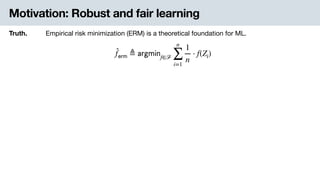
Truth. Study on the “empirical risk minimization” gives a concrete foundation for ML.
̂f 𝖾𝗋𝗆 ≜ 𝖺𝗋𝗀𝗆𝗂𝗇f∈ℱ
n
∑
i=1
1
n
⋅ f(Zi)
Examples. .Robust learning with outliers / noisy labels (high-loss samples are ignored)
Curriculum learning (low-loss samples are prioritized)
Fair ML, with individual fairness criteria (low-loss samples are ignored)
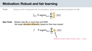
Also Truth. .Modern-day ML is more than just ERM.
-We weigh samples differently, based on their loss values!
̂f ≜ 𝖺𝗋𝗀𝗆𝗂𝗇f∈ℱ
n
∑
i=1
wi ⋅ f(Zi)
[1] e.g., Han et al., “Co-teaching: Robust training of deep neural networks with extremely noisy labels,” NeurIPS 2018.
[2] e.g., Pawan Kumar et al., “Self-paced learning for latent variable models,” NeurIPS 2010.
[3] e.g., Williamson et al., “Fairness risk measures,” ICML 2019.
[1]
[2]
[3]

5. Motivation: Robust and fair learning
Truth. Study on the “empirical risk minimization” gives a concrete foundation for ML.
̂f 𝖾𝗋𝗆 ≜ 𝖺𝗋𝗀𝗆𝗂𝗇f∈ℱ
n
∑
i=1
1
n
⋅ f(Zi)
Also Truth. .Modern-day ML is more than just ERM.
-We weigh samples differently, based on their loss values!
̂f ≜ 𝖺𝗋𝗀𝗆𝗂𝗇f∈ℱ
n
∑
i=1
wi ⋅ f(Zi)
Examples. .Robust learning with outliers / noisy labels (high-loss samples are ignored)
Curriculum learning (low-loss samples are prioritized)
Fair ML, with individual fairness criteria (low-loss samples are ignored)
Question. Can we give convergence guarantees for algorithms with loss-dependent weights?
Challenge. What theoretical framework should we use?

6. Framework: Optimized Certainty Equivalents (OCE)
History. Invented by Ben-Tal and Teboulle (1986) to characterize risk-aversion.
- extends the utility-theoretic perspective of von Neumann and Morgenstern.
Utility curve
(diminishing marginal utility)
Income
(Objective)
Utility
(subjective)
Δ1
Δ2
Δ3

7. Framework: Optimized Certainty Equivalents (OCE)
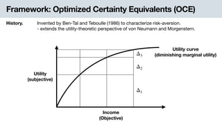
History. Invented by Ben-Tal and Teboulle (1986) to characterize risk-aversion.
- extends the utility-theoretic perspective of von Neumann and Morgenstern.
Definition. Capture the risk-averse behavior using a convex disutility function .ϕ
i.e., negative utility
𝗈𝖼𝖾(f, P) ≜ inf
λ∈ℝ
{λ + EP[ϕ(f(Z) − λ)]}
EP[ϕ(f(Z) − λ)]
λ Certain present loss
Uncertain future disutility

8. Framework: Optimized Certainty Equivalents (OCE)
History. Invented by Ben-Tal and Teboulle (1986) to characterize risk-aversion.
- extends the utility-theoretic perspective of von Neumann and Morgenstern.
Definition. Capture the risk-averse behavior using a convex disutility function .ϕ
i.e., negative utility
ML view. .We are penalizing the average loss + deviation!
𝗈𝖼𝖾(f, P) = EP[f(Z)] + inf
λ∈ℝ
{EP[φ(f(Z) − λ)]}
… for some convex .φ(t) = ϕ(t) − t
λ* f(Z𝗁𝗂𝗀𝗁−𝗅𝗈𝗌𝗌)f(Z𝗅𝗈𝗐−𝗅𝗈𝗌𝗌)
“deviation penalty” from the
optimized anchor λ*

9. Framework: Optimized Certainty Equivalents (OCE)
History. Invented by Ben-Tal and Teboulle (1986) to characterize risk-aversion.
- extends the utility-theoretic perspective of von Neumann and Morgenstern.
Definition. Capture the risk-averse behavior using a convex disutility function .ϕ
i.e., negative utility
ML view. .We are penalizing the average loss + deviation!
𝗈𝖼𝖾(f, P) = EP[f(Z)] + inf
λ∈ℝ
{EP[φ(f(Z) − λ)]}
Examples. This framework covers a wide range of “risk-averse” measures of loss.
- Average + variance penalty
- Conditional value-at-risk .(i.e., ignore low-loss samples)
- Entropic risk measure -(i.e., exponentially tilted loss).
Note: OCE is complementary to rank-based approaches
(come to our poster session for details!)
[1] e.g., Maurer and Pontil, “Empirical Bernstein bounds and sample variance penalization,” COLT 2009.
[2] e.g., Curi et al., “Adaptive sampling for stochastic risk-averse learning,” NeurIPS 2020.
[3] e.g., Li et al., “Tilted empirical risk minimization,” arXiv 2020.
[1]
[2]
[3]

10. Framework: Optimized Certainty Equivalents (OCE)
History. Invented by Ben-Tal and Teboulle (1986) to characterize risk-aversion.
- extends the utility-theoretic perspective of von Neumann and Morgenstern.
Definition. Capture the risk-averse behavior using a convex disutility function .ϕ
i.e., negative utility
ML view. .We are penalizing the average loss + deviation!
𝗈𝖼𝖾(f, P) = EP[f(Z)] + inf
λ∈ℝ
{EP[φ(f(Z) − λ)]}
Examples. This framework covers a wide range of “risk-averse” measures of loss.
- Average + variance penalty
- Conditional value-at-risk .(i.e., ignore low-loss samples)
- Entropic risk measure -(i.e., exponentially tilted loss).
Inverted OCE. A new notion to address “risk-seeking” algorithms (e.g., ignore high-loss samples)
𝗈𝖼𝖾(f, P) ≜ EP[f(Z)] − inf
λ∈ℝ
{EP[φ(λ − f(Z))]}

11. Results: Two learning bounds.
What we do. We analyze the empirical OCE minimization procedure:
Just as Vapnik&Chervonenkis studies “empirical risk minimization.”
we also give inverted OCE version.
̂f 𝖾𝗈𝗆 ≜ 𝖺𝗋𝗀𝗆𝗂𝗇f∈ℱ
𝗈𝖼𝖾(f, Pn)

12. Results: Two learning bounds.
In a nutshell. We give learning bounds of two different type.
What we do. We analyze the empirical OCE minimization procedure:
Just as Vapnik&Chervonenkis studies “empirical risk minimization.”
we also give inverted OCE version.
𝗈𝖼𝖾( ̂f 𝖾𝗈𝗆, P) − inf
f∈ℱ
𝗈𝖼𝖾(f, P) ≈ 𝒪
(
𝖫𝗂𝗉(ϕ) ⋅ 𝖼𝗈𝗆𝗉(ℱ)
n )
EP[ ̂f 𝖾𝗈𝗆(Z)] − inf
f∈ℱ
EP[f(Z)] ≈ 𝒪
(
𝖼𝗈𝗆𝗉(ℱ)
n )
Theorem 6. Excess expected loss bound
Theorem 3. Excess OCE bound
(come to our poster session for details!)
̂f 𝖾𝗈𝗆 ≜ 𝖺𝗋𝗀𝗆𝗂𝗇f∈ℱ
𝗈𝖼𝖾(f, Pn)

13. Results: Two learning bounds.
In a nutshell. We give learning bounds of two different type.
What we do. We analyze the empirical OCE minimization procedure:
Just as Vapnik&Chervonenkis studies “empirical risk minimization.”
we also give inverted OCE version.
Theorem 6. Excess expected loss bound
Theorem 3. Excess OCE bound
Also… We also discover the relationship to sample variance penalization (SVP) procedure,
and find that SVP is a nice baseline strategy for batch-based OCE minimization.
(come to our poster session for details!)
̂f 𝖾𝗈𝗆 ≜ 𝖺𝗋𝗀𝗆𝗂𝗇f∈ℱ
𝗈𝖼𝖾(f, Pn)
𝗈𝖼𝖾( ̂f 𝖾𝗈𝗆, P) − inf
f∈ℱ
𝗈𝖼𝖾(f, P) ≈ 𝒪
(
𝖫𝗂𝗉(ϕ) ⋅ 𝖼𝗈𝗆𝗉(ℱ)
n )
EP[ ̂f 𝖾𝗈𝗆(Z)] − inf
f∈ℱ
EP[f(Z)] ≈ 𝒪
(
𝖼𝗈𝗆𝗉(ℱ)
n )

14. Results: Two learning bounds.
In a nutshell. We give learning bounds of two different type.
What we do. We analyze the empirical OCE minimization procedure:
Just as Vapnik&Chervonenkis studies “empirical risk minimization.”
we also give inverted OCE version.
Theorem 6. Excess expected loss bound
Theorem 3. Excess OCE bound
Also… We also discover the relationship to sample variance penalization (SVP) procedure,
and find that SVP is a nice baseline strategy for batch-based OCE minimization.
(come to our poster session for details!)
̂f 𝖾𝗈𝗆 ≜ 𝖺𝗋𝗀𝗆𝗂𝗇f∈ℱ
𝗈𝖼𝖾(f, Pn)
𝗈𝖼𝖾( ̂f 𝖾𝗈𝗆, P) − inf
f∈ℱ
𝗈𝖼𝖾(f, P) ≈ 𝒪
(
𝖫𝗂𝗉(ϕ) ⋅ 𝖼𝗈𝗆𝗉(ℱ)
n )
EP[ ̂f 𝖾𝗈𝗆(Z)] − inf
f∈ℱ
EP[f(Z)] ≈ 𝒪
(
𝖼𝗈𝗆𝗉(ℱ)
n )
TL;DR. . - We give OCE-based theoretical framework to address robust/fair ML.
-- We give excess risk bounds for empirical OCE minimizers.
- Further implications of our theoretical results…
- Proof ideas…
- Experiment details…
- Comparisons with alternative frameworks…
Come to our zoom session for interesting details, including…