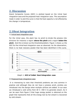
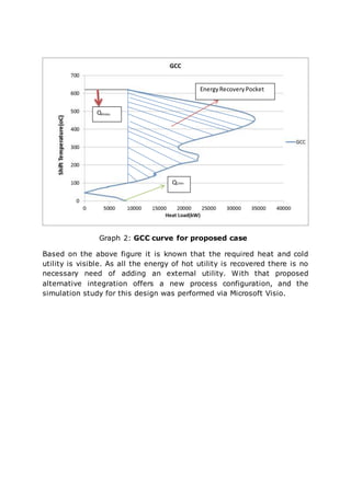
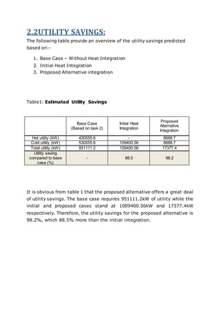
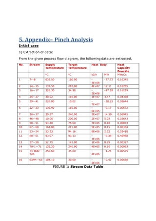
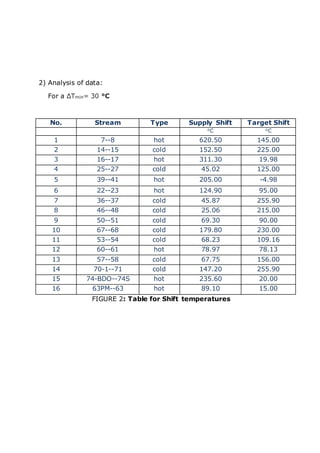
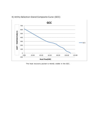
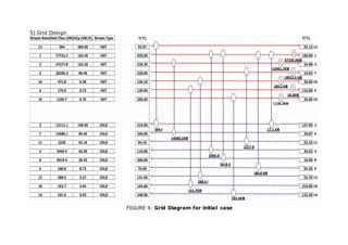
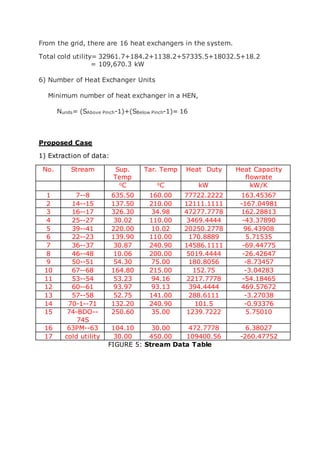
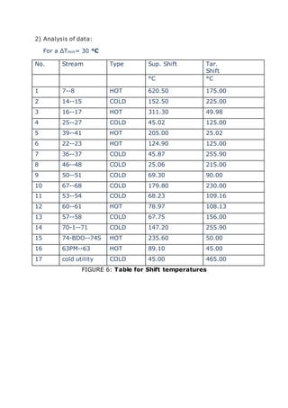
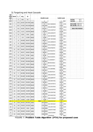
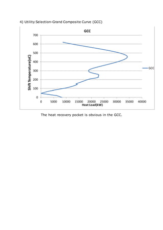
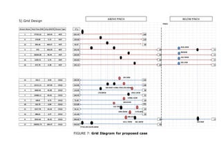
H82 PLD:
Heat Exchanger Network
Synthesis
Group number 31
Group Member
Adnaan Malak (012117)
Chumley Fernando (011493)
Santhosh Ganesan (009074)
Lecturer
Dr. Denny K. S. Ng
1. Introduction
In industrial plants these days, one of the major problems that have been
identified is the huge amount consumption of energy for production
purposes. This is found to be a reason that contributes to increase in
operational and production cost of industries. At a specific level, energy is
consumed and rejected at another level. Most of the industrial processes
involve the heat transfer from a stream to another stream or from a
utility to a stream. In order to overcome this highly rated problem, pinch
analysis is used which is known to be successful for investigation of this
matter and efficient design of heat exchangers networks. Pinch analysis
basically is used to analyse the heat flow of a process based on the
fundamentals of thermodynamics. It has the tools known as the hot and
cold composite curves which are the overall heat demand release of an
industrial process. This are used to identify the possible heat recovery
which would lower the energy cost of industrial plants.
2. Discussion
Grand Composite Curves (GCC) is plotted based on the initial heat
integration case and the proposed heat integration case. The assumption
made in order to plot this curve is that the heat capacity is not affected by
the change in temperature.
2.1Heat Integration
1) Initial heat integration case
For the initial case, the plant has no pinch to divide the process into
divisions for instance a region above the pinch and a region below the
pinch. And this is known as the threshold problem. Figure 1 shows us the
GCC for the initial heat integration case as observed. As the observation,
there is no heat recovery pocket that has been identified in this curve.
Graph 1: GCC of Initial Heat Integration case
2) Proposed heat integration case
It is interesting to note that threshold problems are very common in
practice and although they do not have a process pinch, pinches are
introduced into the design when multiple utilities are added. In our case
we introduced a cold utility from 30◦ C -450◦ C to generate steam. As it
can be seen from figure 2 that huge energy pocket is obtained on the
graph that represents that all the energy lost by hot stream is recovered
by cold stream.
-100
0
100
200
300
400
500
600
700
0.00 20.00 40.00 60.00 80.00 100.00 120.00
GCC
GCC
Heat Flow(kW)
SHIFTTEMPERATURE(₀C)
Graph 2: GCC curve for proposed case
Based on the above figure it is known that the required heat and cold
utility is visible. As all the energy of hot utility is recovered there is no
necessary need of adding an external utility. With that proposed
alternative integration offers a new process configuration, and the
simulation study for this design was performed via Microsoft Visio.
EnergyRecoveryPocket
QHmin
QCmin
2.2UTILITY SAVINGS:
The following table provide an overview of the utility savings predicted
based on:-
1. Base Case – Without Heat Integration
2. Initial Heat Integration
3. Proposed Alternative integration
Table1: Estimated Utility Savings
It is obvious from table 1 that the proposed alternative offers a great deal
of utility savings. The base case requires 951111.2kW of utility while the
initial and proposed cases stand at 1009400.56kW and 17377.4kW
respectively. Therefore, the utility savings for the proposed alternative is
98.2%, which 88.5% more than the initial integration.
Base Case
(Based on task 2)
Initial Heat
Integration
Proposed
Alternative
Integration
Hot utility (kW) 420555.6 - 8688.7
Cold utility (kW) 530555.6 109400.56 8688.7
Total utility (kW) 951111.2 109400.56 17377.4
Utility saving
compared to base
case (%)
- 88.5 98.2
3. Conclusion
The problem that is encountered the most by almost all of the industrial
plant is the huge amount consumption of energy. This problem can be
solved by introducing pinch analysis. This technology has been really
efficient by reducing the amount of energy consumed and at the same
time managed to reduce the capital cost as well of many industrial plants.
This is though proven in the proposed case where huge amount of energy
was saved using this solution. Through the use of this very efficient
technology, energy was conversed, heat recovery was maximized, energy
consumption was reduced and the reduction of capital cost.
4. Reference:
1. Smith, R. (2005). Chemical Process Design and Integration. New
York: John Wiley & Sons
2. Polley, G.T. and Hegg, P.J. (1999). Don’t let the Pinch pinch you.
ABI/INFORM Trade & Industry.
3. Pinch Technology Basic for Engineers; article
5. Appendix– Pinch Analysis
Initial case
1) Extraction of data:
From the given process flow diagram, the following data are extracted.
No. Stream Supply
Temperature
Target
Temperature
Heat Duty Heat
Capacity
flowrate
oC oC kJ/h MW MW/Oc
1 7--8 635.50 160.00 -
3E+08
-77.72 0.16345
2 14--15 137.50 210.00 4E+07 12.11 0.16705
3 16--17 326.30 34.98 -
2E+08
-47.28 0.16229
4 25--27 30.02 110.00 1E+07 3.47 0.04338
5 39--41 220.00 10.02 -
7E+07
-20.25 0.09644
6 22--23 139.90 110.00 -
6E+05
-0.17 0.00572
7 36--37 30.87 240.90 5E+07 14.59 0.06945
8 46--48 10.06 200.00 2E+07 5.02 0.02643
9 50--51 54.30 75.00 7E+05 0.18 0.00873
10 67--68 164.80 215.00 5E+05 0.15 0.00304
11 53--54 53.23 94.16 8E+06 2.22 0.05418
12 60--61 93.97 93.13 -
1E+06
-0.39 0.46958
13 57--58 52.75 141.00 1E+06 0.29 0.00327
14 70-1--71 132.20 240.90 4E+05 0.10 0.00093
15 74-BDO--
74S
250.60 35.00 -
4E+06
-1.24 0.00575
16 63PM--63 104.10 30.00 -
2E+06
-0.47 0.00638
FIGURE 1: Stream Data Table
2) Analysis of data:
For a ΔTmin= 30 °C
FIGURE 2: Table for Shift temperatures
No. Stream Type Supply Shift Target Shift
oC oC
1 7--8 hot 620.50 145.00
2 14--15 cold 152.50 225.00
3 16--17 hot 311.30 19.98
4 25--27 cold 45.02 125.00
5 39--41 hot 205.00 -4.98
6 22--23 hot 124.90 95.00
7 36--37 cold 45.87 255.90
8 46--48 cold 25.06 215.00
9 50--51 cold 69.30 90.00
10 67--68 cold 179.80 230.00
11 53--54 cold 68.23 109.16
12 60--61 hot 78.97 78.13
13 57--58 cold 67.75 156.00
14 70-1--71 cold 147.20 255.90
15 74-BDO--74S hot 235.60 20.00
16 63PM--63 hot 89.10 15.00
3) Targeting and Heat Cascade
FIGURE 3: Problem Table Algorithm (PTA) for initial case
Shift
Temperature
Interval T(i+1)-Ti mCpnet dH
Infeasible Cascade Feasible Cascade
°C °C kW/K kW Hot Pinch 635.5 °C
620.5 PINCH ▼ 0 ▼ 0 Cold Pinch 605.5 °C
1 309.2 163.5 50539.8762 surplus 50539.88 50539.88
311.3 ▼ 50539.88 ▼ 50539.88 Min Hot Utility 0.0 kW
2 55.4 325.7 18046.0959 surplus 18046.1 18046.1 Min Cold Utility109400.56 kW
255.9 ▼ 68585.97 ▼ 68585.97
3 20.3 255.4 5183.8139 surplus 5183.814 5183.814 SINGLE PINCH PROBLEM
235.6 ▼ 73769.79 ▼ 73769.79
4 5.6 261.1 1462.2182 surplus 1462.218 1462.218 THRESHOLD PROBLEM
230 ▼ 75232 ▼ 75232
5 5 258.1 1290.3378 surplus 1290.338 1290.338
225 ▼ 76522.34 ▼ 76522.34
6 10 91.0 910.1776 surplus 910.1776 910.1776
215 ▼ 77432.52 ▼ 77432.52
7 10 64.6 645.9128 surplus 645.9128 645.9128
205 ▼ 78078.43 ▼ 78078.43
8 25.2 161.0 4057.9651 surplus 4057.965 4057.965
179.8 ▼ 82136.4 ▼ 82136.4
9 23.8 164.1 3904.9419 surplus 3904.942 3904.942
156 ▼ 86041.34 ▼ 86041.34
10 3.5 160.8 562.8098 surplus 562.8098 562.8098
152.5 ▼ 86604.15 ▼ 86604.15
11 5.3 327.9 1737.6189 surplus 1737.619 1737.619
147.2 ▼ 88341.77 ▼ 88341.77
12 2.2 328.8 723.33 surplus 723.33 723.33
145 ▼ 89065.1 ▼ 89065.1
13 20 165.3 3306.6541 surplus 3306.654 3306.654
125 ▼ 92371.75 ▼ 92371.75
14 0.1 122.0 12.1954 surplus 12.19538 12.19538
124.9 ▼ 92383.95 ▼ 92383.95
15 15.74 127.7 2009.5125 surplus 2009.512 2009.512
109.16 ▼ 94393.46 ▼ 94393.46
16 14.16 73.5 1040.5405 surplus 1040.541 1040.541
95 ▼ 95434 ▼ 95434
17 5 67.8 338.8458 surplus 338.8458 338.8458
90 ▼ 95772.85 ▼ 95772.85
18 0.9 59.0 53.1311 surplus 53.13113 53.13113
89.1 ▼ 95825.98 ▼ 95825.98
19 10.13 65.4 662.6525 surplus 662.6525 662.6525
78.97 ▼ 96488.63 ▼ 96488.63
20 0.84 535.0 449.3929 surplus 449.3929 449.3929
78.13 ▼ 96938.02 ▼ 96938.02
21 8.83 65.4 577.6132 surplus 577.6132 577.6132
69.3 ▼ 97515.64 ▼ 97515.64
22 1.07 74.1 79.3399 surplus 79.33988 79.33988
68.23 ▼ 97594.98 ▼ 97594.98
23 0.48 128.3 61.6004 surplus 61.60035 61.60035
67.75 ▼ 97656.58 ▼ 97656.58
24 21.88 131.6 2879.5054 surplus 2879.505 2879.505
45.87 ▼ 100536.1 ▼ 100536.1
25 0.85 201.1 170.8944 surplus 170.8944 170.8944
45.02 ▼ 100707 ▼ 100707
26 19.96 244.4 4878.8448 surplus 4878.845 4878.845
25.06 ▼ 105585.8 ▼ 105585.8
27 5.06 270.9 1370.5393 surplus 1370.539 1370.539
20 ▼ 106956.4 ▼ 106956.4
28 0.02 265.1 5.3021 surplus 5.302149 5.302149
19.98 ▼ 106961.7 ▼ 106961.7
29 4.98 102.8 512.0403 surplus 512.0403 512.0403
15 ▼ 107473.7 ▼ 107473.7
30 19.98 96.4 1926.8528 surplus 1926.853 1926.853
-4.98 ▼ 109400.6 ▼ 109400.6
4) Utility Selection-Grand Composite Curve (GCC)
The heat recovery pocket is merely visible in the GCC.
-100
0
100
200
300
400
500
600
700
0.00 20.00 40.00 60.00 80.00 100.00 120.00
GCC
GCC
Heat Flow(kW)
SHIFTTEMPERATURE(₀C)
5) Grid Design
FIGURE 4: Grid Diagram for initial case
Stream NameHeat Flow (kW)mCp (kW/K) Stream Type T(o
C) T(o
C)
12 394 469.05 HOT 93.97 93.13 12
1 77722.2 163.45 HOT 635.00 160.00 1
57335.5KW
3 47277.8 162.30 HOT 326.30 34.98 3
32961.7KW
5 20250.3 96.40 HOT 220.00 10.02 7
18032.5 kW
16 472.8 6.38 HOT 104.10 30.00 16
184.2 kW
6 170.9 5.72 HOT 139.90 110.00 5
18.2KW
15 1239.7 5.75 HOT 250.60 35.00 15
1138.2KW
2 12111.1 166.90 COLD 210.00 137.50 2
394 kW 11717.1 kW
7 14586.1 69.45 COLD 240.90 30.87 6
14586.1KW
11 2220 54.18 COLD 94.16 53.23 11
. 2217.8KW
4 3469.4 43.39 COLD 110.00 30.02 4
3469.4KW
8 5019.4 26.43 COLD 200.00 10.06 8
5019.4 kW
9 180.8 8.73 COLD 75.00 54.30 9
180.8 kW
13 288.6 3.27 COLD 141.00 52.75 13
288.6 kW
10 152.7 3.04 COLD 164.80 215.00 10
152.7KW
14 101.5 0.93 COLD 240.90 132.20 14
101.5KW
C
C
C
C
C
C
From the grid, there are 16 heat exchangers in the system.
Total cold utility= 32961.7+184.2+1138.2+57335.5+18032.5+18.2
= 109,670.3 kW
6) Number of Heat Exchanger Units
Minimum number of heat exchanger in a HEN,
Nunits= (SAbove Pinch-1)+(SBelow Pinch-1)= 16
Proposed Case
1) Extraction of data:
No. Stream Sup.
Temp
Tar. Temp Heat Duty Heat Capacity
flowrate
oC oC kW kW/K
1 7--8 635.50 160.00 77722.2222 163.45367
2 14--15 137.50 210.00 12111.1111 -167.04981
3 16--17 326.30 34.98 47277.7778 162.28813
4 25--27 30.02 110.00 3469.4444 -43.37890
5 39--41 220.00 10.02 20250.2778 96.43908
6 22--23 139.90 110.00 170.8889 5.71535
7 36--37 30.87 240.90 14586.1111 -69.44775
8 46--48 10.06 200.00 5019.4444 -26.42647
9 50--51 54.30 75.00 180.8056 -8.73457
10 67--68 164.80 215.00 152.75 -3.04283
11 53--54 53.23 94.16 2217.7778 -54.18465
12 60--61 93.97 93.13 394.4444 469.57672
13 57--58 52.75 141.00 288.6111 -3.27038
14 70-1--71 132.20 240.90 101.5 -0.93376
15 74-BDO--
74S
250.60 35.00 1239.7222 5.75010
16 63PM--63 104.10 30.00 472.7778 6.38027
17 cold utility 30.00 450.00 109400.56 -260.47752
FIGURE 5: Stream Data Table
2) Analysis of data:
For a ΔTmin= 30 °C
FIGURE 6: Table for Shift temperatures
No. Stream Type Sup. Shift Tar.
Shift
°C °C
1 7--8 HOT 620.50 175.00
2 14--15 COLD 152.50 225.00
3 16--17 HOT 311.30 49.98
4 25--27 COLD 45.02 125.00
5 39--41 HOT 205.00 25.02
6 22--23 HOT 124.90 125.00
7 36--37 COLD 45.87 255.90
8 46--48 COLD 25.06 215.00
9 50--51 COLD 69.30 90.00
10 67--68 COLD 179.80 230.00
11 53--54 COLD 68.23 109.16
12 60--61 HOT 78.97 108.13
13 57--58 COLD 67.75 156.00
14 70-1--71 COLD 147.20 255.90
15 74-BDO--74S HOT 235.60 50.00
16 63PM--63 HOT 89.10 45.00
17 cold utility COLD 45.00 465.00
3) Targeting and Heat Cascade
FIGURE 7: Problem Table Algorithm (PTA) for proposed case
4) Utility Selection-Grand Composite Curve (GCC)
The heat recovery pocket is obvious in the GCC.
0
100
200
300
400
500
600
700
0 5000 10000 15000 20000 25000 30000 35000 40000
ShiftTemperature(oC)
Heat Load(kW)
GCC
GCC
5) Grid Design
FIGURE 7: Grid Diagram for proposed case
PINCH
Stream Name Heat Flow (kW) mCp (kW/K) Stream Type T(o
c)
1 77722.22 163.45 HOT 635.50 160
6 170.89 5.72 HOT 139.00 110
12 394.44 469.57 HOT 93.97 93
3531.6KW
3 473 162.29 HOT 326.30 60 35
4822KW
5 20250.28 96.44 HOT 220.00 60 10
143.75KW
15 1239.72 5.75 HOT 250.60 60 35
335.1KW
16 472.78 6.38 HOT 104.10 60 30
101.5KW
14 101.5 0.93 COLD 240.90 132
2 12111.11 167.05 COLD 210.00 138
394.4KW 11588.17KW128.54KW
4 3469.44 43.38 COLD 110.00 30
170.89KW 2454.15KW
7 14586.11 69.45 COLD 240.90 31
14586.11KW
9 180.8 8.73 COLD 75.00 54
180.81KW
10 152.75 3.04 COLD 215.00 165
152.75KW
11 2217.78 54.18 COLD 94.16 53
1095.95KW 1170.6KW
13 288.61 3.27 COLD 141.00 53
288.61KW
8 5019.44 26.43 COLD 200.00 30 10
4211.74KW 281.36KW 525.9kW
17 106955.75 260.47 COLD 450.00 30
77722.2KW31678.34KW
H
H
H
H
H
H
H
H
C
C
C
C
ABOVE PINCH BELOW PINCH
From the grid, there are 22 heat exchangers in the system.
Total cold utility= 3531.6+4822+ 143.75+335.1
= 8688.7 kW
Total hot utility = 101.5+128.54+2454.15+180.81+152.75+
1170.6+288.61+4211.74
= 8688.7 kW
6) Number of Heat Exchanger Units
Minimum number of heat exchanger in a HEN,
Nunits= (SAbove Pinch-1)+(SBelow Pinch-1)= 22
PLD-FINAL-REPORT
PLD-FINAL-REPORT

PLD-FINAL-REPORT

  • 1.
    H82 PLD: Heat ExchangerNetwork Synthesis Group number 31 Group Member Adnaan Malak (012117) Chumley Fernando (011493) Santhosh Ganesan (009074) Lecturer Dr. Denny K. S. Ng
  • 2.
    1. Introduction In industrialplants these days, one of the major problems that have been identified is the huge amount consumption of energy for production purposes. This is found to be a reason that contributes to increase in operational and production cost of industries. At a specific level, energy is consumed and rejected at another level. Most of the industrial processes involve the heat transfer from a stream to another stream or from a utility to a stream. In order to overcome this highly rated problem, pinch analysis is used which is known to be successful for investigation of this matter and efficient design of heat exchangers networks. Pinch analysis basically is used to analyse the heat flow of a process based on the fundamentals of thermodynamics. It has the tools known as the hot and cold composite curves which are the overall heat demand release of an industrial process. This are used to identify the possible heat recovery which would lower the energy cost of industrial plants.
  • 3.
    2. Discussion Grand CompositeCurves (GCC) is plotted based on the initial heat integration case and the proposed heat integration case. The assumption made in order to plot this curve is that the heat capacity is not affected by the change in temperature. 2.1Heat Integration 1) Initial heat integration case For the initial case, the plant has no pinch to divide the process into divisions for instance a region above the pinch and a region below the pinch. And this is known as the threshold problem. Figure 1 shows us the GCC for the initial heat integration case as observed. As the observation, there is no heat recovery pocket that has been identified in this curve. Graph 1: GCC of Initial Heat Integration case 2) Proposed heat integration case It is interesting to note that threshold problems are very common in practice and although they do not have a process pinch, pinches are introduced into the design when multiple utilities are added. In our case we introduced a cold utility from 30◦ C -450◦ C to generate steam. As it can be seen from figure 2 that huge energy pocket is obtained on the graph that represents that all the energy lost by hot stream is recovered by cold stream. -100 0 100 200 300 400 500 600 700 0.00 20.00 40.00 60.00 80.00 100.00 120.00 GCC GCC Heat Flow(kW) SHIFTTEMPERATURE(₀C)
  • 5.
    Graph 2: GCCcurve for proposed case Based on the above figure it is known that the required heat and cold utility is visible. As all the energy of hot utility is recovered there is no necessary need of adding an external utility. With that proposed alternative integration offers a new process configuration, and the simulation study for this design was performed via Microsoft Visio. EnergyRecoveryPocket QHmin QCmin
  • 6.
    2.2UTILITY SAVINGS: The followingtable provide an overview of the utility savings predicted based on:- 1. Base Case – Without Heat Integration 2. Initial Heat Integration 3. Proposed Alternative integration Table1: Estimated Utility Savings It is obvious from table 1 that the proposed alternative offers a great deal of utility savings. The base case requires 951111.2kW of utility while the initial and proposed cases stand at 1009400.56kW and 17377.4kW respectively. Therefore, the utility savings for the proposed alternative is 98.2%, which 88.5% more than the initial integration. Base Case (Based on task 2) Initial Heat Integration Proposed Alternative Integration Hot utility (kW) 420555.6 - 8688.7 Cold utility (kW) 530555.6 109400.56 8688.7 Total utility (kW) 951111.2 109400.56 17377.4 Utility saving compared to base case (%) - 88.5 98.2
  • 7.
    3. Conclusion The problemthat is encountered the most by almost all of the industrial plant is the huge amount consumption of energy. This problem can be solved by introducing pinch analysis. This technology has been really efficient by reducing the amount of energy consumed and at the same time managed to reduce the capital cost as well of many industrial plants. This is though proven in the proposed case where huge amount of energy was saved using this solution. Through the use of this very efficient technology, energy was conversed, heat recovery was maximized, energy consumption was reduced and the reduction of capital cost.
  • 8.
    4. Reference: 1. Smith,R. (2005). Chemical Process Design and Integration. New York: John Wiley & Sons 2. Polley, G.T. and Hegg, P.J. (1999). Don’t let the Pinch pinch you. ABI/INFORM Trade & Industry. 3. Pinch Technology Basic for Engineers; article
  • 9.
    5. Appendix– PinchAnalysis Initial case 1) Extraction of data: From the given process flow diagram, the following data are extracted. No. Stream Supply Temperature Target Temperature Heat Duty Heat Capacity flowrate oC oC kJ/h MW MW/Oc 1 7--8 635.50 160.00 - 3E+08 -77.72 0.16345 2 14--15 137.50 210.00 4E+07 12.11 0.16705 3 16--17 326.30 34.98 - 2E+08 -47.28 0.16229 4 25--27 30.02 110.00 1E+07 3.47 0.04338 5 39--41 220.00 10.02 - 7E+07 -20.25 0.09644 6 22--23 139.90 110.00 - 6E+05 -0.17 0.00572 7 36--37 30.87 240.90 5E+07 14.59 0.06945 8 46--48 10.06 200.00 2E+07 5.02 0.02643 9 50--51 54.30 75.00 7E+05 0.18 0.00873 10 67--68 164.80 215.00 5E+05 0.15 0.00304 11 53--54 53.23 94.16 8E+06 2.22 0.05418 12 60--61 93.97 93.13 - 1E+06 -0.39 0.46958 13 57--58 52.75 141.00 1E+06 0.29 0.00327 14 70-1--71 132.20 240.90 4E+05 0.10 0.00093 15 74-BDO-- 74S 250.60 35.00 - 4E+06 -1.24 0.00575 16 63PM--63 104.10 30.00 - 2E+06 -0.47 0.00638 FIGURE 1: Stream Data Table
  • 10.
    2) Analysis ofdata: For a ΔTmin= 30 °C FIGURE 2: Table for Shift temperatures No. Stream Type Supply Shift Target Shift oC oC 1 7--8 hot 620.50 145.00 2 14--15 cold 152.50 225.00 3 16--17 hot 311.30 19.98 4 25--27 cold 45.02 125.00 5 39--41 hot 205.00 -4.98 6 22--23 hot 124.90 95.00 7 36--37 cold 45.87 255.90 8 46--48 cold 25.06 215.00 9 50--51 cold 69.30 90.00 10 67--68 cold 179.80 230.00 11 53--54 cold 68.23 109.16 12 60--61 hot 78.97 78.13 13 57--58 cold 67.75 156.00 14 70-1--71 cold 147.20 255.90 15 74-BDO--74S hot 235.60 20.00 16 63PM--63 hot 89.10 15.00
  • 11.
    3) Targeting andHeat Cascade FIGURE 3: Problem Table Algorithm (PTA) for initial case Shift Temperature Interval T(i+1)-Ti mCpnet dH Infeasible Cascade Feasible Cascade °C °C kW/K kW Hot Pinch 635.5 °C 620.5 PINCH ▼ 0 ▼ 0 Cold Pinch 605.5 °C 1 309.2 163.5 50539.8762 surplus 50539.88 50539.88 311.3 ▼ 50539.88 ▼ 50539.88 Min Hot Utility 0.0 kW 2 55.4 325.7 18046.0959 surplus 18046.1 18046.1 Min Cold Utility109400.56 kW 255.9 ▼ 68585.97 ▼ 68585.97 3 20.3 255.4 5183.8139 surplus 5183.814 5183.814 SINGLE PINCH PROBLEM 235.6 ▼ 73769.79 ▼ 73769.79 4 5.6 261.1 1462.2182 surplus 1462.218 1462.218 THRESHOLD PROBLEM 230 ▼ 75232 ▼ 75232 5 5 258.1 1290.3378 surplus 1290.338 1290.338 225 ▼ 76522.34 ▼ 76522.34 6 10 91.0 910.1776 surplus 910.1776 910.1776 215 ▼ 77432.52 ▼ 77432.52 7 10 64.6 645.9128 surplus 645.9128 645.9128 205 ▼ 78078.43 ▼ 78078.43 8 25.2 161.0 4057.9651 surplus 4057.965 4057.965 179.8 ▼ 82136.4 ▼ 82136.4 9 23.8 164.1 3904.9419 surplus 3904.942 3904.942 156 ▼ 86041.34 ▼ 86041.34 10 3.5 160.8 562.8098 surplus 562.8098 562.8098 152.5 ▼ 86604.15 ▼ 86604.15 11 5.3 327.9 1737.6189 surplus 1737.619 1737.619 147.2 ▼ 88341.77 ▼ 88341.77 12 2.2 328.8 723.33 surplus 723.33 723.33 145 ▼ 89065.1 ▼ 89065.1 13 20 165.3 3306.6541 surplus 3306.654 3306.654 125 ▼ 92371.75 ▼ 92371.75 14 0.1 122.0 12.1954 surplus 12.19538 12.19538 124.9 ▼ 92383.95 ▼ 92383.95 15 15.74 127.7 2009.5125 surplus 2009.512 2009.512 109.16 ▼ 94393.46 ▼ 94393.46 16 14.16 73.5 1040.5405 surplus 1040.541 1040.541 95 ▼ 95434 ▼ 95434 17 5 67.8 338.8458 surplus 338.8458 338.8458 90 ▼ 95772.85 ▼ 95772.85 18 0.9 59.0 53.1311 surplus 53.13113 53.13113 89.1 ▼ 95825.98 ▼ 95825.98 19 10.13 65.4 662.6525 surplus 662.6525 662.6525 78.97 ▼ 96488.63 ▼ 96488.63 20 0.84 535.0 449.3929 surplus 449.3929 449.3929 78.13 ▼ 96938.02 ▼ 96938.02 21 8.83 65.4 577.6132 surplus 577.6132 577.6132 69.3 ▼ 97515.64 ▼ 97515.64 22 1.07 74.1 79.3399 surplus 79.33988 79.33988 68.23 ▼ 97594.98 ▼ 97594.98 23 0.48 128.3 61.6004 surplus 61.60035 61.60035 67.75 ▼ 97656.58 ▼ 97656.58 24 21.88 131.6 2879.5054 surplus 2879.505 2879.505 45.87 ▼ 100536.1 ▼ 100536.1 25 0.85 201.1 170.8944 surplus 170.8944 170.8944 45.02 ▼ 100707 ▼ 100707 26 19.96 244.4 4878.8448 surplus 4878.845 4878.845 25.06 ▼ 105585.8 ▼ 105585.8 27 5.06 270.9 1370.5393 surplus 1370.539 1370.539 20 ▼ 106956.4 ▼ 106956.4 28 0.02 265.1 5.3021 surplus 5.302149 5.302149 19.98 ▼ 106961.7 ▼ 106961.7 29 4.98 102.8 512.0403 surplus 512.0403 512.0403 15 ▼ 107473.7 ▼ 107473.7 30 19.98 96.4 1926.8528 surplus 1926.853 1926.853 -4.98 ▼ 109400.6 ▼ 109400.6
  • 12.
    4) Utility Selection-GrandComposite Curve (GCC) The heat recovery pocket is merely visible in the GCC. -100 0 100 200 300 400 500 600 700 0.00 20.00 40.00 60.00 80.00 100.00 120.00 GCC GCC Heat Flow(kW) SHIFTTEMPERATURE(₀C)
  • 13.
    5) Grid Design FIGURE4: Grid Diagram for initial case Stream NameHeat Flow (kW)mCp (kW/K) Stream Type T(o C) T(o C) 12 394 469.05 HOT 93.97 93.13 12 1 77722.2 163.45 HOT 635.00 160.00 1 57335.5KW 3 47277.8 162.30 HOT 326.30 34.98 3 32961.7KW 5 20250.3 96.40 HOT 220.00 10.02 7 18032.5 kW 16 472.8 6.38 HOT 104.10 30.00 16 184.2 kW 6 170.9 5.72 HOT 139.90 110.00 5 18.2KW 15 1239.7 5.75 HOT 250.60 35.00 15 1138.2KW 2 12111.1 166.90 COLD 210.00 137.50 2 394 kW 11717.1 kW 7 14586.1 69.45 COLD 240.90 30.87 6 14586.1KW 11 2220 54.18 COLD 94.16 53.23 11 . 2217.8KW 4 3469.4 43.39 COLD 110.00 30.02 4 3469.4KW 8 5019.4 26.43 COLD 200.00 10.06 8 5019.4 kW 9 180.8 8.73 COLD 75.00 54.30 9 180.8 kW 13 288.6 3.27 COLD 141.00 52.75 13 288.6 kW 10 152.7 3.04 COLD 164.80 215.00 10 152.7KW 14 101.5 0.93 COLD 240.90 132.20 14 101.5KW C C C C C C
  • 14.
    From the grid,there are 16 heat exchangers in the system. Total cold utility= 32961.7+184.2+1138.2+57335.5+18032.5+18.2 = 109,670.3 kW 6) Number of Heat Exchanger Units Minimum number of heat exchanger in a HEN, Nunits= (SAbove Pinch-1)+(SBelow Pinch-1)= 16 Proposed Case 1) Extraction of data: No. Stream Sup. Temp Tar. Temp Heat Duty Heat Capacity flowrate oC oC kW kW/K 1 7--8 635.50 160.00 77722.2222 163.45367 2 14--15 137.50 210.00 12111.1111 -167.04981 3 16--17 326.30 34.98 47277.7778 162.28813 4 25--27 30.02 110.00 3469.4444 -43.37890 5 39--41 220.00 10.02 20250.2778 96.43908 6 22--23 139.90 110.00 170.8889 5.71535 7 36--37 30.87 240.90 14586.1111 -69.44775 8 46--48 10.06 200.00 5019.4444 -26.42647 9 50--51 54.30 75.00 180.8056 -8.73457 10 67--68 164.80 215.00 152.75 -3.04283 11 53--54 53.23 94.16 2217.7778 -54.18465 12 60--61 93.97 93.13 394.4444 469.57672 13 57--58 52.75 141.00 288.6111 -3.27038 14 70-1--71 132.20 240.90 101.5 -0.93376 15 74-BDO-- 74S 250.60 35.00 1239.7222 5.75010 16 63PM--63 104.10 30.00 472.7778 6.38027 17 cold utility 30.00 450.00 109400.56 -260.47752 FIGURE 5: Stream Data Table
  • 15.
    2) Analysis ofdata: For a ΔTmin= 30 °C FIGURE 6: Table for Shift temperatures No. Stream Type Sup. Shift Tar. Shift °C °C 1 7--8 HOT 620.50 175.00 2 14--15 COLD 152.50 225.00 3 16--17 HOT 311.30 49.98 4 25--27 COLD 45.02 125.00 5 39--41 HOT 205.00 25.02 6 22--23 HOT 124.90 125.00 7 36--37 COLD 45.87 255.90 8 46--48 COLD 25.06 215.00 9 50--51 COLD 69.30 90.00 10 67--68 COLD 179.80 230.00 11 53--54 COLD 68.23 109.16 12 60--61 HOT 78.97 108.13 13 57--58 COLD 67.75 156.00 14 70-1--71 COLD 147.20 255.90 15 74-BDO--74S HOT 235.60 50.00 16 63PM--63 HOT 89.10 45.00 17 cold utility COLD 45.00 465.00
  • 16.
    3) Targeting andHeat Cascade FIGURE 7: Problem Table Algorithm (PTA) for proposed case
  • 17.
    4) Utility Selection-GrandComposite Curve (GCC) The heat recovery pocket is obvious in the GCC. 0 100 200 300 400 500 600 700 0 5000 10000 15000 20000 25000 30000 35000 40000 ShiftTemperature(oC) Heat Load(kW) GCC GCC
  • 18.
    5) Grid Design FIGURE7: Grid Diagram for proposed case PINCH Stream Name Heat Flow (kW) mCp (kW/K) Stream Type T(o c) 1 77722.22 163.45 HOT 635.50 160 6 170.89 5.72 HOT 139.00 110 12 394.44 469.57 HOT 93.97 93 3531.6KW 3 473 162.29 HOT 326.30 60 35 4822KW 5 20250.28 96.44 HOT 220.00 60 10 143.75KW 15 1239.72 5.75 HOT 250.60 60 35 335.1KW 16 472.78 6.38 HOT 104.10 60 30 101.5KW 14 101.5 0.93 COLD 240.90 132 2 12111.11 167.05 COLD 210.00 138 394.4KW 11588.17KW128.54KW 4 3469.44 43.38 COLD 110.00 30 170.89KW 2454.15KW 7 14586.11 69.45 COLD 240.90 31 14586.11KW 9 180.8 8.73 COLD 75.00 54 180.81KW 10 152.75 3.04 COLD 215.00 165 152.75KW 11 2217.78 54.18 COLD 94.16 53 1095.95KW 1170.6KW 13 288.61 3.27 COLD 141.00 53 288.61KW 8 5019.44 26.43 COLD 200.00 30 10 4211.74KW 281.36KW 525.9kW 17 106955.75 260.47 COLD 450.00 30 77722.2KW31678.34KW H H H H H H H H C C C C ABOVE PINCH BELOW PINCH
  • 19.
    From the grid,there are 22 heat exchangers in the system. Total cold utility= 3531.6+4822+ 143.75+335.1 = 8688.7 kW Total hot utility = 101.5+128.54+2454.15+180.81+152.75+ 1170.6+288.61+4211.74 = 8688.7 kW 6) Number of Heat Exchanger Units Minimum number of heat exchanger in a HEN, Nunits= (SAbove Pinch-1)+(SBelow Pinch-1)= 22