This document provides an overview of modeling piping networks in CHEMCAD software. It discusses how to use pressure nodes to specify known variables like pressures and calculate unknown variables like flowrates. Pressure nodes represent points where pressure changes and can be used to connect unit operations in a piping network. The flowrate and pressure options at each node are described to demonstrate how nodes can be used to properly constrain piping network calculations in CHEMCAD.

1. Adapted from Chemstations CHEMCAD Piping Systems 5.3 User’s Guide and Tutorial dated February 19, 2003.
Prepared by J.E.Edwards of P & I Design Ltd, Teesside, UK. Dated 19 February 2010. MNL076 73 pages
www.chemstations.com www.chemcad.co.uk
PIPING
WORKBOOK
Solving Piping
and
Header Networks
Using CHEMCAD
Version 6.2
• Piping Simulation Methods
• Sizing Piping Components
• Pump Performance Curves
• Piping Networks
• Relief Header Networks
Engineering advanced

2. CHEMCAD 6 Workbook - Pipe and Header Networks
PAGE 2 OF 73
MNL 076 Issued 19 February 2010, Prepared by J.E.Edwards of P&I Design Ltd, Teesside, UK www.chemcad.co.uk
Chapter 1 Introduction to Piping Networks p 3
Chapter 2 Unit Operations in CHEMCAD p 5
Chapter 3 Control Valve Sizing p 11
Chapter 4 Simple Flow Example p 16
Chapter 5 Branched Flow Example p 20
Chapter 6 Relief Flow Piping Example p 25
Chapter 7 Piping Calculation and Design Methods p 29
Energy Equation and Momentum p 29
Friction Factor p 32
Isothermal Flow p 34
Darcy Weisbach p 34
Hazen-Williams p 35
Fritzsche p 35
Two Phase Flow p 36
Baker Two Phase Flow Method p 37
Beggs and Brill Two Phase Flow Method p 43
3K-Darby Method Resistance Method p 54
Heat Loss in Piping Systems p 54
Net Positive Suction Head p 54
Piping Design Considerations p 57
Instrumentation Considerations p 58
Chapter 8 Description of Valves and Fittings p 59
References p 73
WORKBOOK PIPING CONTENTS

3. CHEMCAD 6 Workbook - Pipe and Header Networks
PAGE 3 OF 73
MNL 076 Issued 19 February 2010, Prepared by J.E.Edwards of P&I Design Ltd, Teesside, UK www.chemcad.co.uk
A piping network represents the flow of fluids through several items of equipment. If sufficient variables
(flowrate and pressures) are specified on the network, the unknown variables may be calculated.
For fluid flow through equipment, flowrate may be calculated as a function of the inlet and outlet
pressure. If the user can specify two of the three variables the third is dependent. Specification of
pressure at various points on a piping network diagram allows the system to be described as a system
of dependent equations.
The piping network models in CHEMCAD allow for the simultaneous solution of such a system. If
sufficient constraints are specified, the model will simultaneously solve the flowsheet to converge on the
unknown pressures/flowrates throughout the model.
A simple relief flow system is shown in Figure 1-1.
To size the valve, the pressure out of the valve must be calculated. Known variables are geometry of the
pipe, pressure out of pipe, and flowrate through pipe. A single equation can be used to solve for the
pressure into the pipe as a function of the known variables.
FLOWRATE PRESSURE DEPENDENCY FOR FLUID FLOW
Fluid mechanics allows the calculation of fluid flowrate through a pipe or nozzle as a function of inlet and
outlet pressures. The use of performance curves allows the calculation of fluid flow through a
compressor or pump as a function of inlet and outlet pressures. Figure 1-2 shows UnitOps that may
calculate flowrate as a function of pressures. These UnitOps are referred to as flow scaling UnitOps in
this document because they scale the flowrate of the process stream.
Figure 1-1
CHAPTER 1 INTRODUCTION TO PIPING NETWORKS

4. CHEMCAD 6 Workbook - Pipe and Header Networks
PAGE 4 OF 73
MNL 076 Issued 19 February 2010, Prepared by J.E.Edwards of P&I Design Ltd, Teesside, UK www.chemcad.co.uk
The flow through a pipe section is determined from the general form of the Darcy Weisbach equation:
The flow through a control valve is determined from an equation of the general form:
The flow through an orifice plate is determined from an equation of the general form:
∆P pressure drop
H orifice plate differential pressure
q flow rate
ρ fluid density
d pipe inside diameter
f pipe friction factor
k constant
CV valve sizing coefficient
C orifice discharge coefficient
MODELING PIPE NETWORKS
Piping network systems are used to solve for flowrates and/or pressures around a network of connected
equipment. Typically the user has a flowsheet of equipment connections and various constraints (exit
flowrates, pressure limitations on equipment, etc.) but does not have all the flowrate(s) and/or
pressure(s) for the system.
You may solve a piping network system on a CHEMCAD flowsheet. New models in CHEMCAD allow
you to specify the known variables and solve for the unknown variables on a flowsheet.
The NODE UnitOp allows you to specify the pressure on either side of a UnitOp and calculate the
flowrate as a function of pressure. As an option, you may specify one pressure and the flowrate.
Iterative calculations will solve for the unknown pressure based on the specified pressure and flowrate.
A series of UnitOps may be connected using several nodes. The flowrate through the chain may be
specified at a single point, or calculated based on specified pressures around a UnitOp. It is not
necessary to know the pressures around all UnitOps in the series.
Figure 1-3 shows a simple flare network. There are seven variables of pressure and flowrate. Three of
the variables must be specified.
ρ
Δ
=
P
C
k
q v
L
f
d
P
k
q
5
ρ
Δ
=
ρ
=
h
C
d
k
q 2

5. CHEMCAD 6 Workbook - Pipe and Header Networks
PAGE 5 OF 73
MNL 076 Issued 19 February 2010, Prepared by J.E.Edwards of P&I Design Ltd, Teesside, UK www.chemcad.co.uk
PRESSURE NODES
The piping network calculations solve for pressure at nodes and then iteratively calculate the flowrates
through the network as functions of pressure.
A NODE UnitOp represents a point in the piping network where a change in pressure occurs due to
elevation change, flow through a pipe, or flow through equipment that changes pressure (pump, valve,
etc). A CHEMCAD flowsheet for a piping network uses the pipe UnitOp for piping effects and UnitOps
such as the pump, compressor, and control valve.
For design of a piping network it is necessary to determine pressure between all UnitOps that calculate
pressure as a function of flowrate. The NODE UnitOp sets the pressure on one side of a UnitOp that
calculates pressure as a function of flowrate.
The pressure at a node may be specified by the user or calculated by CHEMCAD. The flowrate(s) in
and out of a node may be specified or calculated. The flowrates may be specified at the NODE UnitOp,
or calculated as dependent on adjacent UnitOps.
The NODE UnitOp sets a fixed value on the flowsheet. For piping network calculations there are points
on the flowsheet where either the pressure or flowrate is known. The NODE UnitOp allows specification
of the known variable and calculation of the unknown variable.
To learn the concepts for specifying a node, look at a system of two nodes surrounding a UnitOp. This is
shown in Figure 2-1.
The inlet pressure (P1), outlet pressure (P2), and flowrate (F) through the pipe are the three variables. A
single equation constrains the system. Specification of any two of the variables allows CHEMCAD to
solve for the third variable.
If pressure is specified at the first node and either node specifies flowrate, the pressure of the second
node is variable. CHEMCAD will vary the pressure of the second node until flowrate as a function of
pressure around the pipe equals the specified flowrate. The pressure may vary at either node.
The pressure of a feed or product stream of known flowrate may be adjusted by adjacent nodes.
Specifying P1 as fixed pressure specifies the pressure of stream 1 as P=P1. If pressure at both nodes is
specified, the flowrate through the UnitOp is a dependent variable.
The variable flowrate may be either the feed stream or product stream. In the NODE UnitOp, specify the
location where flowrate is a variable. Use mode free outlet or free inlet to specify whether the inlet or
outlet flow is calculated. The model will cascade this flowrate upstream and downstream of the UnitOp.
The pressure of streams attached to a NODE UnitOp will be set to the pressure of the node. The
flowrates through a network will all be set to the calculated flowrate through a node. You may specify
(N– 1) flowrates on a flowsheet, where N is the total of feed and product streams on the flowsheet. The
calculated flowrate will be passed through nodes that use the dependent flowrate. You will receive an
error message if you attempt to specify or calculate two conflicting flowrates through a system with two
separate nodes.
CHAPTER 2 UNIT OPERATIONS IN CHEMCAD

6. CHEMCAD 6 Workbook - Pipe and Header Networks
PAGE 6 OF 73
MNL 076 Issued 19 February 2010, Prepared by J.E.Edwards of P&I Design Ltd, Teesside, UK www.chemcad.co.uk
Flowrate Options at Node
The flowrate for an inlet or outlet stream may be manipulated by a node. The node acts by manipulating
the flowrate of the adjacent UnitOp. The pressure settings for the nodes on either side of the adjacent
UnitOp contribute to the flowrate manipulation.
Fixed Flowrates at Node
Using a fixed inlet flowrate for a node specifies the flowrate through the upstream UnitOp. The pressure
on one side (node) of the UnitOp must be variable. An exception is when a node is acting as a mixer or
divider for N streams and the one stream is variable. In this situation the pressure can be fixed or
variable for both nodes.
The Fixed outlet flowrate for a node specifies the flowrate through the downstream UnitOp. This setting
is similar to fixed inlet.
The Current flowrate setting for an inlet stream is similar to fixed inlet. The current flowrate uses the
flowrate currently stored for the inlet stream rather than a specified value in the node.
Variable Flowrates at Node
Using free inlet for a node specifies that the feed stream flowrate is a calculated variable. The node will
manipulate the upstream feed flowrate to solve the system. The free inlet specification works best on a
node connected to a Feed stream but it may be placed elsewhere on the flowsheet.
If the outlet flow is specified, the free inlet specification allows the feed to be calculated to maintain mass
balance. Only one free inlet specification is allowed per feed stream.
The free outlet stream for a node is similar to the free inlet setting. Using free outlet specifies that the
product stream flowrate is a calculated variable. The node will manipulate the product flowrate to solve
the system. The free outlet specification works best on a node connected to a product stream but it may
be placed elsewhere on the flowsheet.
If the inlet flow to a system is specified, the free outlet specification allows the product to be calculated
to maintain mass balance. Only one free outlet specification is allowed per product stream.
If you attempt to specify too many free outlet or free inlet streams, CHEMCAD will issue a warning
message and reset the extra specifications to flow set by UnitOp.
The flow set by UnitOp setting indicates that the flowrate is controlled by the adjacent UnitOp. The
UnitOp may be calculating flowrate as a function of pressure. The UnitOp may be using the flowrate
calculated by another UnitOp.
Mass Balance Limitations for Flowrate Calculation
Only one UnitOp on a branch of the network may calculate flowrate. If the nodes adjacent to a UnitOp
both use flow set by UnitOp and fixed pressure, the calculated flowrate may be used as the flowrate at a
free inlet or free outlet node. If the nodes adjacent to a UnitOp use flow set by UnitOp but do not both fix
pressure, the flowrate through the UnitOp is calculated elsewhere on the flowsheet.
The behaviour of Flow set by UnitOp depends on the flowrate specifications of other nodes on the
branch. To illustrate, we consider a system from Figure 2-1.
The inlet to SECOND NODE is flow set by UnitOp.
The node will use the flowrate from the pipe.
If the feed stream is fixed inlet, this is the flowrate for the pipe.
If the feed stream is free inlet and the product streams are fixed flowrate, the free inlet feed flowrate is
set by mass balance. The free inlet is the flow through the pipe. If the feed stream is free inlet, one
product stream is free outlet, and both nodes are fixed pressure, the free inlet and free outlet are set by
the pipe flowrate. The pipe flowrate is set to the critical flowrate for the given pipe with the specified inlet
and outlet pressures.

7. CHEMCAD 6 Workbook - Pipe and Header Networks
PAGE 7 OF 73
MNL 076 Issued 19 February 2010, Prepared by J.E.Edwards of P&I Design Ltd, Teesside, UK www.chemcad.co.uk
Figure 2-2 demonstrates various acceptable combinations of flow settings for nodes. shows the
flowsheet for this job.
NODE AS DIVIDER
A node may be used as a divider. Outlet streams from the node will be at the pressure of the node.
Outlet streams will all have the same temperature and composition but flowrates may differ.
The flowrates may be specified as set by pipe/valve or fixed flowrates. Only one outlet stream flowrate
may be free outlet.
A Node specified as a divider is shown in Figure 2-3. The second node acts as a divider (two product
streams). For N inlet and outlet streams it is necessary to specify (N-1) values.
For the second node, specify the flowrate of two of the three connected streams. Allow the third stream
to be free for mass balance requirements.
If both outlet flowrates are specified, the inlet stream must be calculated as free inlet at node 1 to
maintain mass balance. If one outlet is calculated as free outlet by the node, the inlet stream may be
flow set by pipe if both nodes are fixed pressure.

8. CHEMCAD 6 Workbook - Pipe and Header Networks
PAGE 8 OF 73
MNL 076 Issued 19 February 2010, Prepared by J.E.Edwards of P&I Design Ltd, Teesside, UK www.chemcad.co.uk
PRESSURE NODE DIALOG SCREEN
Mode
Select Fixed pressure to set the pressure at the node and allow flowrate to be variable. Select Variable
Pressure to leave pressure variable at the node.
Pressure at Node
Specify the pressure for Fixed Pressure mode. For Variable Pressure mode the calculated pressure is
displayed. Optionally you may specify an estimate for Variable Pressure mode. The estimate will be
replaced with calculated result.
Minimum Pressure
Specify upper bound for pressure at the node for Variable Pressure mode. Specifying minimum
and maximum pressure will speed calculations.
Maximum Pressure
Specify a lower bound for pressure at the node for Variable Pressure mode. Specifying
minimum and maximum pressure will speed calculations.
Elevation
Specify the elevation at the node. The elevation will add a pressure contribution based on height.
Specifications are absolute. The default elevation is zero. Positive and negative specifications are
allowed.
Flowrate options (Inlet)
Stream Number
The CHEMCAD stream number for the connected inlet stream is displayed.
Flowrate Option
Select the specification for the stream.
Fixed Mole Rate/Fixed Mass Rate/Fixed Volume Rate
The stream flowrate is a known variable. The stream flowrate is set to the specified value
during calculations.
Flow set by Pipe/Valve/Pump
The stream flowrate is a dependent variable. Stream flowrate will be calculated by the adjacent
(upstream) UnitOp to satisfy pressure requirements.
Free Inlet Stream
Specifies the inlet stream to the node is a dependent variable. The inlet stream flowrate will be
calculated for mass balance of the node / flowsheet. Only one inlet to a node may be Free inlet.
Specification of Free inlet is not allowed for a stream that is downstream of another node. Use
Free Inlet Stream to specify a variable feed stream.
Use Current Stream Rate
The stream flowrate is a known variable. The stream flowrate is set to the current flowrate of
the stream.
Value
Specify a fixed flowrate for Fixed mole rate, fixed mass rate, or fixed volume rate. Fixed Volume Rate
specifies the total Actual Volume Rate of the stream. Engineering Units for flow are displayed; the
flowsheet units of mole rate, mass rate, and liquid flowrate are used.
Flowrate Options (Outlet)
Stream Number
The CHEMCAD ID number for the connected outlet stream is displayed. A value of N/A indicates no
stream is connected at this outlet.
Flowrate Option
Select the specification for the stream.
Fixed Mole Rate/Fixed Mass Rate/Fixed Volume Rate
The stream flowrate is a known variable. The stream flowrate is set to the specified value
during calculations.
Flow set by Pipe/Valve /Pump
The stream flowrate is a dependent variable. Stream flowrate will be calculated by the adjacent
(downstream) UnitOp to satisfy pressure requirements.
Free Outlet Stream
The stream flowrate from the node is a dependent variable. The Free Outlet stream flowrate
will be calculated for mass balance of the node / flowsheet. Only one outlet from a node may
be Free outlet. Specification of Free outlet is not allowed for a stream that is upstream of
another node. Use Free Outlet Stream to specify a variable product stream.
Value
Specify a fixed flowrate for Fixed mole rate, fixed mass rate, or fixed volume rate. Fixed Volume Rate
specifies the total Actual Volume Rate of the stream. Engineering Units for flow are displayed; the
flowsheet units of mole rate, mass rate, and liquid flowrate are used.

9. CHEMCAD 6 Workbook - Pipe and Header Networks
PAGE 9 OF 73
MNL 076 Issued 19 February 2010, Prepared by J.E.Edwards of P&I Design Ltd, Teesside, UK www.chemcad.co.uk
PIPE SIMULATOR
Description
The pipe simulator UnitOp in CHEMCAD is used to model pressure drop of a fluid through a pipe.
Piping Network Modes of Pipe Simulator
Sizing Option 5 (Given Size Pin and Pout calculate flowrate) of the pipe UnitOp allows calculation of
flowrate through the pipe as function of geometry, inlet and outlet pressure. The outlet pressure of a
known pipe is a function of inlet pressure and flowrate. Any two of these three variables are independent
variables.
A NODE UnitOp can use (or calculate) the flowrate from an adjacent pipe as the flowrate for a stream
connected to the node. Use stream option Flow set by pipe/valve for the node.
The use of Sizing Option 5 for a pipe UnitOp connected to a node creates one variable on the Piping
Network. The variable may be the flowrate through the pipe or the pressure at either end of the pipe.
If the node is fixed pressure, the pressure of the node will be used for the pressure of the attached pipe.
If the nodes on either side of a pipe are fixed pressure with Flow set by pipe for the pipe UnitOp
streams, the flowrate through the pipe is calculated based on the inlet and outlet pressures. If one of the
nodes on either side of the pipe is variable pressure, the variable pressure is calculated based on the
fixed pressure (from the other node) and flowrate. The flowrate may be a fixed value set by either node,
or it may be specified elsewhere on the flowsheet.
PUMP
Description
The Pump UnitOp has a characteristic equation mode that calculates outlet pressure as a function of
inlet pressure and flowrate.
Piping Network Modes of Pump UnitOp
A NODE UnitOp can use (or calculate) the flowrate from an adjacent pump as the flowrate for a stream
connected to the node. Use stream option Flow set by pipe/valve for the node.
The use of the characteristic equation mode specifies one unknown on the Piping Network. The
unknown may be the flowrate through the pump or the pressure at either end of the pump. The node
connected to the pump acts to constrain the unknown.
VALVES
Description
There are two UnitOps that may be used to represent valves in a Piping Network simulation. The Valve
(VALV) UnitOp allows an arbitrary adiabatic pressure change of pressure between nodes.
Piping Network Modes of Valve UnitOp
Use a valve UnitOp when a valve changes to or from a variable pressure node. The valve UnitOp is
used to change the pressure of the stream to match the pressure calculated by the pressure node. The
valve does not adjust flowrate unless turned off. Do not specify an outlet pressure for the valve.
CONTROL VALVE
Description
The PID control valve may be used in manual control model on a piping network. The valve flow
coefficient (Cv) must be specified. The Control Valve (CVAL) UnitOp has three modes for manual
control.
Piping Network Modes of Control Valve
Mode Fix valve position and adjust flow rate is used to calculate flowrate as a function of Cv, valve
position, inlet pressure, and outlet pressure. The downstream node is fixed P and free inlet stream, or
variable P and free outlet stream w/inlet flow set by UnitOp.
COMPRESSOR
Piping Network Modes of Compressor
The Compressor UnitOp in mode 5 Specify Performance Curves calculates outlet pressure as a function
of volumetric flowrate, efficiency, and head of gas. Volumetric flowrate and head to the compressor are
functions of the mass flowrate and inlet pressure of the compressor.

10. CHEMCAD 6 Workbook - Pipe and Header Networks
PAGE 10 OF 73
MNL 076 Issued 19 February 2010, Prepared by J.E.Edwards of P&I Design Ltd, Teesside, UK www.chemcad.co.uk
NODE AS MIXER
A node may be used as a mixer. The inlet streams to the node will all have the same pressure as the
node. Only one inlet stream flowrate may be free inlet.
STEADY STATE UNITOPS
Regular steady state UnitOps may be used on a piping network diagram. A constant pressure drop may
be entered for a (non-scaler) steady state UnitOp. Adjacent nodes will recognize pressure drop
specifications on the UnitOp.
Between two nodes there must be one flowrate scaler. A heat exchanger and a pipe can be between
two nodes, as the heat exchanger does not calculate flowrate as a function of pressure. A constant
pressure drop may be specified for the heat exchanger and it will affect the pressure drop between the
two nodes. A heat exchanger cannot be the only UnitOp between two nodes, as the heat exchanger
does not have an effect on pressure.

11. CHEMCAD 6 Workbook - Pipe and Header Networks
PAGE 11 OF 73
MNL 076 Issued 19 February 2010, Prepared by J.E.Edwards of P&I Design Ltd, Teesside, UK www.chemcad.co.uk
Topics Covered: Control Valve Sizing / Rating, Control Valve UnitOp, Using Nodes
Problem Statement
The example is to size control valves for handling a flow of 113,000 lb/hr of Liquid Ammonia in each line
coming from Divider 1. We wish to select appropriate sized valves and then determine the percent open
for each valve at the rated service. The Example is located in Book1PipingExample1-Sizing.
In the flowsheet Figure 3-1 , inlet stream 1 is at the inlet conditions of -9 degrees F, 225 psig. The
divider splits the 226,000 lb/hr flow into 2 equal flows of 113,000 lb/hr of ammonia.
Control Valve Sizing
To do the initial sizing, run the Divider UnitOp (Right Click>Run This UnitOp) to calculate the flow
information for streams 2 and 3. Both streams should be at -9 degrees F, 225 psig and 113,000 lb/hr of
ammonia.
Next select stream 3 by left clicking on it. The stream is selected when it is shown bracketed by black
squares. Go to the Sizing menu, and select Control valve. The following screen will appear: Enter 15
psig as the Downstream Pressure and press OK and the report in Excel or Word will appear.
CHAPTER 3 CONTROL VALVE SIZING

12. CHEMCAD 6 Workbook - Pipe and Header Networks
PAGE 12 OF 73
MNL 076 Issued 19 February 2010, Prepared by J.E.Edwards of P&I Design Ltd, Teesside, UK www.chemcad.co.uk
The sizing procedure is now repeated for stream 2.
Open control valve 4 by double clicking on it. The screen below will appear; note that the valve
coefficient CV = 36 and the downstream pressure = 15 psig have been automatically entered from the
sizing calculation. Set operating mode to Fix flowrate, adjust valve position. Repeat for valve 5.

13. CHEMCAD 6 Workbook - Pipe and Header Networks
PAGE 13 OF 73
MNL 076 Issued 19 February 2010, Prepared by J.E.Edwards of P&I Design Ltd, Teesside, UK www.chemcad.co.uk
Run the simulation by going to the Run menu and selecting Run All.
To view your results, go to the Results menu, and select UnitOp’s. You should see this dialog asking
for what UnitOps to view:
If you don’t see this, then you already have a unit selected in the flowsheet, and it is showing you a
report for that unit. Close the report, deselect the UnitOps by holding down the shift key while clicking on
the units, and go back to Results, UnitOp’s. You can also deselect UnitOps by left-clicking on a blank
section of the flowsheet.
Select units # 4 and 5 and press the OK button. You will see the following report:
This report shows that valve #4 is at 72.5% open, and valve #5 is at 53.3% open.
By right-clicking on Control valve #5, and selecting View stream properties, we can see how much
vaporization occurs across the valve:
This volume change is why CHEMCAD chose a larger valve for the second stream. With the
vaporization occurring in the valve, a smaller 2-inch valve body would be approaching sonic velocity
through the valve body.

14. CHEMCAD 6 Workbook - Pipe and Header Networks
PAGE 14 OF 73
MNL 076 Issued 19 February 2010, Prepared by J.E.Edwards of P&I Design Ltd, Teesside, UK www.chemcad.co.uk
Flowrate as a function of Pressure
In typical CHEMCAD simulations information flows in one direction: downstream. Upstream conditions
determine the downstream conditions. In most simulations, you simply set the flowrates and pressures
of feed streams. Pressure drops are either calculated based on flow or specified through UnitOps. The
downstream pressures, flowrates, etc. are calculated when the simulation is run.
For piping simulations, flowrate and pressure are dependent on each other. The backpressure on
valves, pipes, and other UnitOps affects the flowrate through the valve. Likewise, the flowrate through a
valve, (or pipe, or pump) determines the downstream pressure. In flow models like the control valve
sizing model, sometimes it is useful to let flowrate vary as a function of the pressure.
For example, assume a process upset caused the pressure in vessel 11 to rise from 15 psig to 30 psig.
Assuming the valve positions don’t change, what is the new inlet flowrate?
In order to answer this question, we need to introduce a special UnitOp called a node. A node is a point
in the simulation that has a pressure, flow coming in, and flow going out. The node units create a
network, solving for flowrate at each point based on the fixed pressures. Nodes are placed on the
flowsheet before and after the control valves. The flowsheet is shown in Figure 3-2 below:
The function of the divider (to split the incoming flow) is now handled by NODE #6. The node will
balance the flowrates such that all streams entering and exiting the node are at the same pressure.
Nodes are also placed between the flash vessels and the control valves. At the nodes we can fix the
pressures, and let the flowrate vary as a function of valve position and pressure difference. Open NODE
6 by double-clicking on it:
The pressure at this node is fixed at 225 psig. The inlet flow is set to Free inlet stream and the two outlet
streams are set to Flow set by UnitOp. Flow into each control valve will be determined by the control
valve Cv valve opening position, and pressure difference across the valve.
The pressure in is set to 30 psig for NODE 9, 0.2 psig for NODE 10. Flow into the node is controlled by
the control valve (Flow set by UnitOp), flow out is a Free Outlet Stream.

15. CHEMCAD 6 Workbook - Pipe and Header Networks
PAGE 15 OF 73
MNL 076 Issued 19 February 2010, Prepared by J.E.Edwards of P&I Design Ltd, Teesside, UK www.chemcad.co.uk
The control valves need to be changed to fix the valve position, and calculate flowrate.
We need to set the Valve mode for each valve to Fix valve position, adjust flowrate in order for the
flowrate to change.
Now we can run the simulation. Go to the Run menu, select Run All. We can view the streams around
NODE 6 by right-clicking on the node and selecting View stream compositions from the menu. The
following report will appear:
The flowrate to Vessel 11 dropped from 113,000 lb/hr to 109138 lb/hr. So we can see the effect of back
pressure on the flowrates through the valves.

16. CHEMCAD 6 Workbook - Pipe and Header Networks
PAGE 16 OF 73
MNL 076 Issued 19 February 2010, Prepared by J.E.Edwards of P&I Design Ltd, Teesside, UK www.chemcad.co.uk
Topics Covered: Pipe UnitOp, NPSH, Math Controllers, Pipe-Control Valve-Orifice Plate Sizing
Problem Statement
The piping system shown must be designed to transport 120 gpm of glacial acetic acid at 70-140F. The
pressure at the inlet is known at 20 psia, the outlet must be no less than 20psia. The piping system and
its individual elements must be sized for design conditions and then rated at operating conditions. Our
goal is to determine the NPSHa and head requirements for future pump selection.
CREATING THE SIMULATION
1) Convert the piping isometric to a CHEMCAD flowsheet. Pipe UnitOps are used to represent entire
sections of piping, including fittings:
2) Using CHEMCAD’s pipe sizing utility (Sizing Menu>Pipes) size the pipes in the network for the
design flowrate of 120 gpm, at 70 F. Use standard schedule 40 pipe. Since the fluid in this system is
subcooled liquid and all flows are constant, this requires us to do only one calculation for the discharge
side. As a rule of thumb, use 1 size larger pipe on the suction of the pump.
The pump discharge line size has been determined using a design velocity of 3 m/s. A discharge line
size of 3 in was selected and for the suction pipe 4 in, a nominal size larger.
CHAPTER 4 SIMPLE FLOW EXAMPLE
Figure 4-1 (PipingExample 2)

17. CHEMCAD 6 Workbook - Pipe and Header Networks
PAGE 17 OF 73
MNL 076 Issued 19 February 2010, Prepared by J.E.Edwards of P&I Design Ltd, Teesside, UK www.chemcad.co.uk
The Pipe UnitOps are configured identically namely Method 2 - Single Phase Flow, Sizing Option 5 –
Given D, PIN, POUT, Calculate Flow, Friction Factor - Churchill and Roughness Factor – Commercial
Steel.
3) The pump discharge stainless steel orifice plate is calculated using the CHEMCAD Sizing > Orifice
tool. It is specified with D and D/2 taps, a design differential of 100 in wc and the thermal expansion 9.6
E-06 in/in ºF. Using the calculated bore hole, the flow resistance factor of the orifice is calculated from
the following, where β= d/D, gives a value 10.719.
C=Cd/(_(1-β
4
))
Kr~K=(1-β
4
)/(C
2
β
4
)
The unrecovered pressure loss is accounted for by adding the calculated Kr in the downstream Pipe
UnitOp User specified window.
4) Size the control valve (Sizing menu>Control valve) using a design pressure drop of 20 psi and a
single seat valve. The Valve position is set to 50% open and the Valve mode option is set to Fix flow,
valve position, calculate Pout.
To size the control valve from an initial build, copy the pipe network inlet stream to the control valve inlet
stream using Specifications > Copy Stream Data and change the pressure to 45 psig. Specify valve with
a 20 psi pressure drop and a correction factor of 0.95.

18. CHEMCAD 6 Workbook - Pipe and Header Networks
PAGE 18 OF 73
MNL 076 Issued 19 February 2010, Prepared by J.E.Edwards of P&I Design Ltd, Teesside, UK www.chemcad.co.uk
5) Assume a 2 psi pressure drop across the heat exchanger. Set the outlet temperature to 140F.
6) Tabulate the valves, fittings, pipe lengths, and elevation changes of each section of pipe. All of our
pipes will use the Single phase method, and the mode should be set to rating. We will be using flanged
fittings throughout.
Pipe #1
1 entrance, well rounded
2 ball valve
4 std elbow 90 degree
1 tee, flow through branch
35 feet piping
-8 foot elevation change
In the example shown no allowance has been made for reducers at the pump suction and discharge
which are normally required; as discussed earlier these can have a significant effect and would require
additional Pipe UnitOps at the pump inlet and discharge.
7) Specify the pump outlet pressure at some arbitrary value (45 psia) and make a trial run. Check the
calculated outlet pressure. We can iterate to find the required pump head.
Pipe #2 (before control valve)
1 swing check valve, clearway
2 ball valves
2 tee, flow through run
1 orifice plate (as determined above)
14 feet piping
14 foot elevation change
Pipe #4 (after E-1515)
1 Ball valve
4 std elbow 90 degree
1 tee 100% flow through run
1 well rounded entrance
1 exit from pipe
157 feet piping
5-foot net elevation change
Pipe #3 (after control valve)
2 ball valve
2 tee, flow through run
3 Std elbow 90 degree
1 exit from pipe
24 feet piping
2 foot elevation change

19. CHEMCAD 6 Workbook - Pipe and Header Networks
PAGE 19 OF 73
MNL 076 Issued 19 February 2010, Prepared by J.E.Edwards of P&I Design Ltd, Teesside, UK www.chemcad.co.uk
USING CONTROLLERS TO SIMPLIFY THE PROBLEM
While manually changing the pump outlet pressure will get us where we need to be, it is easier to let the
program do the work. We’re going to use a UnitOp called a feedback controller (CONT) to adjust this
pressure for us. A Feedback controller in CHEMCAD has nothing to do with process control valves or
PID settings. In a CHEMCAD steady-state model, when we use the term “feedback control” we are
talking about a mathematical controller. It’s a math tool used to adjust a variable on a flowsheet until a
target value reaches our specified value.
Change the flowsheet to include a feedback controller in location shown above.
Specify the Controller mode as a feedback controller. Adjust pump outlet pressure until the pressure
of stream 8 is equal to a constant target of 20 psia. When you are finished, the controller screen should
be as follows:
When you run the simulation, the controller will automatically change the pump outlet pressure until the
pressure leaving the last pipe unit is equal to 20. We now know the head requirements for our pump.
Calculate NPSHa. The net positive suction head is defined as pressure available at pump suction
minus the fluid vapor pressure, expressed in feet of fluid. To calculate this in CHEMCAD is an easy
task. Open the Pump dialog, and put a checkmark where it says Check here to Calculate NPSHa.
Rerun the simulation, and the calculated NPSHa will appear. It is important to the NPSHa calculation
that the inlet piping to the pump be correctly specified. If the piping is not correct, then the pressure at
the inlet may not be correct, and the NPSHa may not be correct.

20. CHEMCAD 6 Workbook - Pipe and Header Networks
PAGE 20 OF 73
MNL 076 Issued 19 February 2010, Prepared by J.E.Edwards of P&I Design Ltd, Teesside, UK www.chemcad.co.uk
Topics: Node UnitOp, Pipe Networks, Pump Selection, Pump UnitOp, Performance Curves
Problem Statement
The previous piping system has been changed; due to the branched flow to the two heat exchangers,
the problem is no longer a simple one. The piping layout, valves and fittings to be used are shown in the
isometric. An orifice plate and control valve is to be installed downstream of the pump to measure and
control flow manually. It is required to determine the branched flow split flow and pressure drops in the
pipe network
Further more the layout is to be tested to ensure an adequate Net Positive Suction Head (NPSH) is
available at the pump suction. The NPSHa is defined as the total pressure available at the pump suction
minus the vapour pressure of fluid at pump suction conditions. If the NPSHa is less than that required by
the pump then cavitation will result.
This example is located in the PipingExample3
The branched flow is a difficult problem to solve using our controller approach. Both exchangers have
different piping and therefore different flowrates. What we need is an approach where we split and
recombine flows, and have the simulation calculate the pressure and flowrates in an iterative manner.
The “node” UnitOp gives us this flexibility.
Figure 5-1
CHAPTER 5 BRANCHED FLOW EXAMPLE

21. CHEMCAD 6 Workbook - Pipe and Header Networks
PAGE 21 OF 73
MNL 076 Issued 19 February 2010, Prepared by J.E.Edwards of P&I Design Ltd, Teesside, UK www.chemcad.co.uk
CREATING THE SIMULATION
For practice you can build the model or use the model called “Piping Example 3 Build” in the electronic
media supplied. It is strongly recommended that you work with a copy of this job. This problem is solved
in CHEMCAD using the Pressure Node UnitOp.
1) Convert the piping isometric to a CHEMCAD flowsheet. Figure 5-2 below shows the equivalent
flowsheet.
The Pressure Node UnitOp can be considered a calculator that adjusts the network pressure at the
node based on the flowrate. In the network the Node sets the pressure between UnitOps that calculates
flow as a function of pressure.
Pipe UnitOps calculate flows based on the Pin and Pout, the Pump and Control Valve UnitOps calculate
flows based on the downstream pressure in the Node; it follows that Node UnitOps located between
UnitOps that calculate the flow are set in the “Flow Set by Upstream and Downstream UnitOps”.
The pressure at the Inlet and Outlet Nodes of this network are fixed at 20 psi and the stream is defined
as Free ie not effected by a UnitOp. The inlet flow could also have been fixed by the Inlet Node.
At a UnitOp there are three variables-PIN, POUT and F; a single equation constrains the system so
specification of any two variables sets the remaining variable.
A node is a point where pressure is uniform. There may be multiple inlets and outlets. The flowrates for
each stream will be balanced by CHEMCAD to reach a single pressure. Pressure may be specified or
allowed to vary.
The Inlet and Outlet Nodes configuration is Fixed Pressure and all other Nodes are Variable Pressure
as shown below:
Figure 5-2

22. CHEMCAD 6 Workbook - Pipe and Header Networks
PAGE 22 OF 73
MNL 076 Issued 19 February 2010, Prepared by J.E.Edwards of P&I Design Ltd, Teesside, UK www.chemcad.co.uk
2) Pipe UnitOps are used to represent entire sections of piping, including fittings. NODE UnitOps are
placed where pressure or flowrate are unknown.
3) Assume a 2 psi pressure drop across each heat exchanger.
4) Tabulate the valves, fittings, pipe lengths, and elevation changes of each section of pipe. We will
be using flanged fittings throughout.
Pipe #1
1 entrance, well rounded
2 ball valve
4 std elbow 90 degree
1 tee, flow through branch
35 feet piping
-8 foot elevation change
5) Pump- At this time we don’t know the pump specifications, so we will set the pump to “Specify
Outlet Pressure” and leave the pressure specification blank. The NODE UnitOps will solve for the
pressure increase, and set the pump outlet pressure accordingly.
6) Setup nodes with appropriate information:
Node 3 Variable pressure, use current stream rate for inlet, flow set by UnitOp for
outlet. Elevation = 20 feet
Node 5 Variable pressure, flow set by UnitOp for both inlet and outlet.
Elevation = 34 feet
Node 7 Variable pressure, flow set by UnitOp for both inlet and outlet.
Elevation = 34 feet
Node 9 Variable pressure, flow set by UnitOp for both inlet and outlet.
Elevation = 34 feet
Node 12 Variable pressure, flow set by UnitOp for both inlet and outlet.
Elevation = 50 feet.
Node 16 Variable pressure, flow set by UnitOp for both inlet and outlet.
Elevation = 38 feet.
Node 18 Variable pressure, flow set by UnitOp for both inlet and outlet.
Elevation = 42 feet.
Node 20
(last node)
Fixed pressure, 20 psia, flow set by UnitOp for inlet, free outlet stream for
outlet. Elevation = 43 feet.
Pipe #2 (before control valve)
1 swing check valve, clearway
2 ball valves
2 tee, flow through run
1 orifice plate (as determined above)
14 feet piping
14 foot elevation change
Pipe #4 (to E-1514)
1 Ball valve
3 std elbow 90 degree
1 tee flow through branch
1 exit from pipe
24 feet piping
16 foot net elevation change
Pipe #3 (after control valve)
1 ball valve
1 tee, flow through run
2 Std elbow 90 degree
10 feet piping
No elevation change
Pipe #5 (from E-1514)
1 Ball valve
3 std elbow 90 degree
1 tee flow through branch
1 well rounded entrance
30 feet piping
-8 foot net elevation change
Pipe #6 (to E-1515)
1 Ball valve
1 std elbow 90 degree
1 tee flow through branch
1 exit from pipe
14 feet piping
4 foot net elevation change
Pipe #8 (to V-1522)
3 std elbow 90 degree
1 exit from pipe
147 feet piping
1 foot net elevation change
Pipe #7 (from E-1515)
1 Ball valve
1 std elbow 90 degree
1 tee flow through run
1 well rounded entrance
10 feet piping
4 foot net elevation change

23. CHEMCAD 6 Workbook - Pipe and Header Networks
PAGE 23 OF 73
MNL 076 Issued 19 February 2010, Prepared by J.E.Edwards of P&I Design Ltd, Teesside, UK www.chemcad.co.uk
RUNNING THE SIMULATION
To run the simulation, press the Run All button or go to the Run menu, and select Run All.
If the simulation doesn’t converge, check all the input settings and run it again. Simulations can be
sensitive to initial estimates and min/max settings in nodes. Convergence is also an iterative process,
so you might need to increase the maximum number of iterations for a given flowsheet.
Once the simulation has run, check the pump UnitOp’s pressure increase. This tells us the head
requirements of our pump. Using this information and our flowrate (120 gpm) we can consult a pump
handbook to determine the correct pump size.
SELECTING A PUMP
Below is an appropriate pump for this application.
The centrifugal pump to be used has the following performance characteristics:
To enter this curve into our pump, select Specify Performance Curve for the pump Mode. Once you do
you have the opportunity to enter multiple speed lines and an operating speed. For our purposes, we’ll
assume we want the pump to be at 1750 RPM, so we enter a single speed line. Press the OK button,
and you will see the following entry screen:
In this screen we can enter as many points as we wish to define our curve. CHEMCAD will fit a
quadratic equation to the points, creating a smooth curve fit to our data.
Now that we have entered the pump performance curve we must add node UnitOps to the suction side
of the pump to allow the flowrate to vary, as shown on flowsheet above. In this way we can calculate
the max flowrate of our system.
Note: when computing the max flow for the system, be sure to open the control valve to 100%.

24. CHEMCAD 6 Workbook - Pipe and Header Networks
PAGE 24 OF 73
MNL 076 Issued 19 February 2010, Prepared by J.E.Edwards of P&I Design Ltd, Teesside, UK www.chemcad.co.uk
RESULTS
The results have been presented in a Graphical User Interface (GUI) format to give a clearer
representation. It has been generated using the CHEMCAD Data Map facility. The graphics and
reporting have been done using Excel.
The results are shown for the control valve fully open. It can be seen there is adequate NPSH and the
discharge pressure criteria have been met. The flow split through the heat exchangers, as a result of the
piping layout and resistances, is predicted to be 56.1 gpm and 117.1 gpm.
Alternatively a report can be generated using the standard CHEMCAD reporting facilities.

25. CHEMCAD 6 Workbook - Pipe and Header Networks
PAGE 25 OF 73
MNL 076 Issued 19 February 2010, Prepared by J.E.Edwards of P&I Design Ltd, Teesside, UK www.chemcad.co.uk
Topics: Branched Network, Compressible flow, Degrees of Freedom, Flare header systems,
Node UnitOp, Pipe UnitOp, Valve UnitOp
FLARE HEADER DESIGN
Flare headers are specialized piping networks desiged to convey relief device flows to a flare where
products are consumed before release to the atmosphere. Using CHEMCAD, we can design and
evaluate flare header networks for many relieving scenarios.
Figure 6-1 shows a simplified flowsheet for a relief header network. The flows and pressures from relief
devices RD0001-RD0008 are previously calculated. The piping network has been designed but not
certified or built. The pipes on this flow diagram represent continuous sections of pipe with various
fittings (elbows, etc).
Problem Statement
• Calculate pressures throughout the network when RD0001, RD0002, RD0007, and RD0008
are in a relief scenario
• Determine if an additional section of 8 inch pipe can be added to the discharge
• Determine effects of a two phase flow scenario through RD0007
• Calculate pressures throughout the network if only three segments of the network have a relief
event
These tasks may be solved using the NODE UnitOp and Piping Network. The problem will be solved
one section of piping at a time. It is easier to tackle the problem if we divide it into smaller problems.
CHAPTER 6 RELIEF FLOW PIPING EXAMPLE
E - 1
E -7
P-2
E - 8
E - 9
E - 1 0
E - 11
E - 1 2
E - 13
R D 0 0 01
R D 0002
R D 000 3
R D 0 004
R D 000 5
R D 00 0 6
R D 000 7
R D 0 008
2 "
3"
4"
3"
6"
2"
3 "
4 "
3" 6 " 6"
8"
2"
3"
4 "
To Flare K/O p ot
Figure 6 -1

26. CHEMCAD 6 Workbook - Pipe and Header Networks
PAGE 26 OF 73
MNL 076 Issued 19 February 2010, Prepared by J.E.Edwards of P&I Design Ltd, Teesside, UK www.chemcad.co.uk
Using results from smaller cases as estimations we can gradually build a complex network, reducing
calculation time.
This example is located in the PipingExample4OneBranch folder.
ONE BRANCH
We begin by drawing one segment of the network as shown in Figure 6-2 below. The intermediate
pressures are unknown/variable and will be solved for. The flowrate and composition from RD0002 is
known. We can specify either the discharge pressure to the system or the entrance pressure at the first
node. We arbitrarily specify the pressure at the first node, making the outlet pressure variable. When
the entire network is drawn we will specify the outlet pressure and recalculate the inlet pressure.
THREE BRANCH
Figure 6-3 shows second and third sections of pipe added to the network representing the flow from
RD0001. A T branch fitting is added to the pipe UnitOp after the node connecting the two sections.
The flowrate from RD0001 is known. The pressure at the first node for RD0001 is variable. If we
consider the RD0001 section a separate section of the pipe, we do not have a degree of freedom to
specify. The pressure at the node where RD0001 flow combines with the RD0002 flow is a dependent
variable for the RD0001 flow; it is calculated by the RD0002 section.
Figure 6 -2

27. CHEMCAD 6 Workbook - Pipe and Header Networks
PAGE 27 OF 73
MNL 076 Issued 19 February 2010, Prepared by J.E.Edwards of P&I Design Ltd, Teesside, UK www.chemcad.co.uk
FOUR BRANCH
A fourth branch is added to the network, shown in Figure 6-4 below. As our flowsheet becomes more
complex, the upper/lower bounds for pressure in the nodes become more important. A more complex
network may require more careful settings of upper and lower bounds.
The flowsheet is run and converged after adding the third and fourth sections. All four branches are on
the network. The calculated discharge pressure is above atmospheric; the network is adequate for this
relieving scenario.
SPECIFYING THE OUTLET PRESSURE
We can now perform a rating case on this network, to determine the minimum pressure at RD0002 for
relief under this scenario.
The pressure on the first section node is changed to variable pressure. The outlet pressure for the
network is changed to fixed pressure. The boundaries on variable pressures are tightened and the
flowsheet is converged to the same results, but with the fixed pressure node changed from inlet to
outlet.
To drop the pressure to 2 psig, one should relax the lower pressure boundaries on variable nodes. By
making several minor adjustments from the current pressure to 2 psig, fewer calculations will be
required.

28. CHEMCAD 6 Workbook - Pipe and Header Networks
PAGE 28 OF 73
MNL 076 Issued 19 February 2010, Prepared by J.E.Edwards of P&I Design Ltd, Teesside, UK www.chemcad.co.uk
ADDITION OF PIPE TO DISCHARGE
A pipe is added to the discharge of the network. The pipe is set to rating mode in CHEMCAD; there is
no need to use nodes around this final pipe. The flowsheet is run; the final pipe calculates outlet
pressure. The design modes of the pipe can be used to determine a required diameter for the pipe if the
required length of pipe is known.
EFFECT OF CLOSED VALVE
The simple valve (VALV) UnitOp in CHEMCAD has a closed setting. This can be used to shutoff the
flow to a section of pipe. In this example we set the valve on RD001 to closed and run the process.
DIFFERENT APPROACHES TO RELIEF PROBLEMS
This has not been an exhaustive study of the use of the piping network calculations in CHEMCAD. This
example process does not represent the only way to study a relief header system; the approach used
was selected for instructional purposes. CHEMCAD’s methods are flexible; you can use a different
approach (fixed pressure inlets, fixed flow on one section, etc) to suit your purposes.

29. CHEMCAD 6 Workbook - Pipe and Header Networks
PAGE 29 OF 73
MNL 076 Issued 19 February 2010, Prepared by J.E.Edwards of P&I Design Ltd, Teesside, UK www.chemcad.co.uk
THE GENERAL ENERGY EQUATION
An expression for the balance or conservation of energy between two points in a system can be derived
as follows:
s
qW
1 1 2
An energy balance results in:
c
c
s
c
c g
MgZ
g
Mv
V
P
U
W
q
g
MgZ
g
Mv
V
P
U 2
2
2
2
2
2
1
2
1
1
1
1
2
2
+
+
+
=
+
+
+
+
+ …(1)
Divide by M and writing the equation in the differential form, on a unit mass basis:
0
W
d
dq
Z
d
gc
g
gc
vdv
P
d
U
d s =
+
+
+
+
⎟
⎟
⎠
⎞
⎜
⎜
⎝
⎛
+
ρ
…(2)
Equation 2 is difficult to apply because U is hard to evaluate. Therefore, equation 2 is converted into
the mechanical energy form.
Since:
ρ
ρ
dP
TdS
h
d
P
d
-
h
d
U
d
+
=
⎟
⎟
⎠
⎞
⎜
⎜
⎝
⎛
=
P
d
dP
TdS
U
d ⎟
⎟
⎠
⎞
⎜
⎜
⎝
⎛
−
+
=
ρ
ρ
…(3)
Replacing equation 3 into equation 2 and rearranging the equation, we obtain:
0
=
+
+
+
+
+ dWs
dq
g
gdZ
g
vdv
dP
TdS
c
c
ρ
…(4)
For an irreversible process,
T
dq
dS
−
≥ or f
P
dq
TdS +
−
=
and assuming no work is done on the system, equation 4 becomes:
0
=
+
+
+ f
c
c
dP
g
gdZ
g
vdv
dP
ρ
…(5)
CHAPTER 7 PIPING CALCULATION AND DESIGN METHODS
c
c
g
MgZ
g
Mv
V
P
U
1
2
1
1
1
1
2
c
c
g
MgZ
g
Mv
V
P
U
2
2
2
2
2
2
2

30. CHEMCAD 6 Workbook - Pipe and Header Networks
PAGE 30 OF 73
MNL 076 Issued 19 February 2010, Prepared by J.E.Edwards of P&I Design Ltd, Teesside, UK www.chemcad.co.uk
if φ
sin
dL
Z = and multiplying by ⎟
⎠
⎞
⎜
⎝
⎛
dL
ρ
Equation 5 becomes:
0
sin =
+
+
+
dL
dP
g
g
dL
dv
g
v
dL
dP f
c
c
ρ
φ
ρ
ρ
…(6)
ENERGY EQUATION NOMENCLATURE
i
U Internal energy
i
i V
P Energy of expansion or contraction
P
Pressure
V
Volume
2gc
Mv2
i
Kinetic energy
M
Mass
v
Velocity
gc
Gravity constant
gc
Z
Mg i
Potential energy
Z
Elevation above datum
q Heat additions (losses)
s
W Work done on the fluid
h
Enthalpy
ρ
Density
T
Temperature
S
Entropy
Pf Losses due to irreversible processes like friction.
L Length
sin Φ Some angle of elevation

31. CHEMCAD 6 Workbook - Pipe and Header Networks
PAGE 31 OF 73
MNL 076 Issued 19 February 2010, Prepared by J.E.Edwards of P&I Design Ltd, Teesside, UK www.chemcad.co.uk
CONSERVATION OF MOMENTUM
Conservation of Linear Momentum Equation:
( ) ( ) θ
ρ
π
τ
ρ
ρ sin
2
g
A
D
dL
dP
v
dL
d
v
dL
d
−
−
−
=
+ …(7)
At steady state:
o
sin
A
D
L
d
P
d
L
d
v
d
g
2
ρ
π
τ
ρ
−
−
=
⎟
⎠
⎞
⎜
⎝
⎛
and
( )
L
d
v
d
v
L
d
v
d
v
L
d
v
d 2
•
+
=
⎟
⎠
⎞
⎜
⎝
⎛
ρ
ρ
ρ
then,
( ) o
sin
A
D
L
d
P
d
L
d
v
d
v
L
d
v
d
v g
ρ
π
τ
ρ
ρ
−
−
=
+
At steady state
( ) 0
L
d
v
d
=
ρ
, replacing this value and rearranging the above equation, we obtain:
o
sin
A
D
L
d
v
d
v
L
d
P
d
g
ρ
π
τ
ρ +
+
= …(8)
CONSERVATION OF MOMENTUM NOMENCLATURE
L
Length
τ Shear stress coefficient
ρ
Density
π Pi
v
velocity
D
Diameter
L
d
P
d
Pressure loss
A
Cross sectional area
P
Pressure o
sin
g
ρ Gravitational loss
A
D
π
τ Shear stress loss (friction) L
d
v
d
v
ρ
Acceleration losses. Normally negligible and
significant only if compressible flow exits at low
pressure.
An evaluation of wall shear stress (or friction losses) can be accomplished by defining a dimensionless
friction factor f, the Darcy-Weisbach(or Darcy or Moody 0r Blasius) friction factor:
2
2
v
f w
ρ
τ
= manipulation produces the Darcy-Weisbach equation:
D
2
v
f
4
D
D
8
v
f
dL
dP 2
2
2
f
ρ
π
π
ρ
=
⎟
⎟
⎠
⎞
⎜
⎜
⎝
⎛
⎟
⎟
⎠
⎞
⎜
⎜
⎝
⎛
=
⎟
⎠
⎞
⎜
⎝
⎛
…(9)
WALL SHEAR STRESS NOMENCLATURE
w
τ Wall shear stress
f
d
P
d
⎟
⎟
⎠
⎞
⎜
⎜
⎝
⎛
L
Pressure loss due to friction
2
2
v
ρ Fluid kinetic energy
ρ Density
P Pressure v velocity
L Length D Diameter

32. CHEMCAD 6 Workbook - Pipe and Header Networks
PAGE 32 OF 73
MNL 076 Issued 19 February 2010, Prepared by J.E.Edwards of P&I Design Ltd, Teesside, UK www.chemcad.co.uk
FRICTION FACTOR DETERMINATION
For Laminar Flow an analytical expression can be derived for the Darcy friction factor:
Re
64
f = or
Re
16
fF =
For Turbulent flow, the friction factor is developed from Colebrook:
2
vf
Re
7
.
18
D
2
Log
2
74
.
1
f
−
⎭
⎬
⎫
⎩
⎨
⎧
⎟
⎠
⎞
⎜
⎝
⎛
+
−
=
ρ
In terms of a Darcy-Weisbach or Moody friction factor:
fF
4
f = and
D
g
2
v
f
dL
dP
c
2
f
ρ
=
⎟
⎠
⎞
⎜
⎝
⎛
Acceleration Component
7) The acceleration component will be equal to zero for constant area, incompressible flow.
8) For any flow condition in which a velocity change occurs, such as compressible flow, a pressure
drop will occur in the direction of velocity increase.
The Jain equation is used to solve directly for the Darcy Weisbach friction factor f for a full-flowing
circular pipe. It is an approximation of the implicit Colebrook-White equation.
The equation was found to match the Colebrook-White equation within 1.0% for 10
-6
< ε/D < 10
-2
and
5000 < Re < 10
8
. However the Churchill method is applicable for all values of ε/D and Re.
FRICTION FACTOR NOMENCLATURE
f Darcy Friction factor (CHEMCAD uses this form throughout)
Re
Reynolds number
ρ Density
D Diameter
v velocity
fF
Fanning friction factor
f
d
P
d
⎟
⎟
⎠
⎞
⎜
⎜
⎝
⎛
L
Pressure loss due to friction
gc
Gravitational constant
ε Pipe roughness
For an independent check of the friction factor the Moody diagram is used. Knowing the pipe flow Re
and the pipe roughness coefficient ε (units of m or ft), giving the relative roughness ε/D (consistent
units), the friction factor can be determined. The laminar flow line formula will allow verification of the
diagram friction factor being used. Check friction factor at Re=1000; if Darcy f=0.064 and if Fanning
fF=0.016.

33. CHEMCAD 6 Workbook - Pipe and Header Networks
PAGE 33 OF 73
MNL 076 Issued 19 February 2010, Prepared by J.E.Edwards of P&I Design Ltd, Teesside, UK www.chemcad.co.uk
Moody Diagram – Darcy Friction Factor
Example Friction factor for cast iron pipe D = 500mm, ε = 0.5 mm (ε/D = 0.001) with Re of 300000 is
0.026
The diagram below shows Colebrook, Churchill, Darcy-Churchill and Blasius friction factors for smooth
pipes. The Blasius Equation being the most accurate for smooth pipes. estimating turbulent pressure
drops. Smooth pipe conditions are very well defined.

34. CHEMCAD 6 Workbook - Pipe and Header Networks
PAGE 34 OF 73
MNL 076 Issued 19 February 2010, Prepared by J.E.Edwards of P&I Design Ltd, Teesside, UK www.chemcad.co.uk
ISOTHERMAL FLOW EQUATION
The isothermal flow equation is solved as follows:
2
1
1
2
2
2
1
2
1
4
ln
2
12
024
.
1337
⎪
⎪
⎭
⎪
⎪
⎬
⎫
⎪
⎪
⎩
⎪
⎪
⎨
⎧
⎥
⎦
⎤
⎢
⎣
⎡ −
⎥
⎥
⎥
⎥
⎥
⎦
⎤
⎢
⎢
⎢
⎢
⎢
⎣
⎡
⎟
⎟
⎠
⎞
⎜
⎜
⎝
⎛
+
⎟
⎠
⎞
⎜
⎝
⎛
=
P
P
P
P
P
D
L
f
D
w
ρ
2
1
1
2
2
2
1
2
1
2
1
2 ln
2
12
⎪
⎭
⎪
⎬
⎫
⎪
⎩
⎪
⎨
⎧
⎥
⎦
⎤
⎢
⎣
⎡ −
⎥
⎦
⎤
⎢
⎣
⎡
⎟
⎟
⎠
⎞
⎜
⎜
⎝
⎛
+
⎟
⎠
⎞
⎜
⎝
⎛
−
=
P
P
P
P
P
D
L
f
P
P
( )
RT
P
MW
=
ρ
ISOTHERMAL EQUATION NOMENCLATURE
w Gas flow, lb/h
ρ Gas density, lb/ft3
D Terminal gas pressure, psia
L Pipe length, ft.
P1 Initial gas pressure, psia
P2 Terminal gas pressure, psia
f Friction factor
MW Molecular weight of gas
P Gas pressure, psia
R Gas constant, 10.73
T Absolute, temperature
o
R
THE DARCY-WEISBACH EQUATION
( )
c
g
D
fLv
P
2
144
2
ρ
=
Δ
DARCY-WEISBACH NOMENCLATURE
ΔP Pressure drop
ρ Density
f Darcy Friction factor
L Pipe length
v Velocity
D Diameter
gc Gravitational constant

35. CHEMCAD 6 Workbook - Pipe and Header Networks
PAGE 35 OF 73
MNL 076 Issued 19 February 2010, Prepared by J.E.Edwards of P&I Design Ltd, Teesside, UK www.chemcad.co.uk
HAZEN-WILLIAMS EQUATION
The Hazen-Williams equation is used for the design of water sprinkler systems for fire protection. The
National Fire Protection Association mandates the design of such systems.
The Hazen and Williams formula for flow of water is:
54
.
0
2
1
2.63
L
P
P
C
D
0.442
Q ⎟
⎟
⎠
⎞
⎜
⎜
⎝
⎛ −
=
HAZEN-WILLIAMS EQUATION NOMENCLATURE
Q Volumetric flow of water, gal/min
D Inside diameter, ft
C
140 for new steel pipe
130 for new cast iron pipe
100 is often used for design purposes to account for pipe fouling
P Pressure, psia
L Length of pipe segment, ft
FRITZSCHE EQUATION
The Fritzsche equation is used to calculate the pressure drops in steam systems:
97
.
4
7
85
.
1
100
)
10
(
82
.
210
D
w
P
ρ
=
Δ
FRITZCHE EQUATION NOMENCALTURE
ΔP100 Pressure drop per 100 feet, psi
w Mass flowrate, lb/hr.
ρ Density, lb/ft
3
D Inside diameter of pipe, in.

36. CHEMCAD 6 Workbook - Pipe and Header Networks
PAGE 36 OF 73
MNL 076 Issued 19 February 2010, Prepared by J.E.Edwards of P&I Design Ltd, Teesside, UK www.chemcad.co.uk
TWO PHASE FLOW
DEFINITIONS FOR TWO PHASE FLOW
Liquid Holdup
segment
pipe
of
volume
segment
pipe
a
in
liquid
of
volume
HL =
Gas Holdup or Gas Void Fraction
L
H
1
Hg −
=
No-Slip Liquid Holdup
v
L
L
Q
Q
Q
L
+
=
λ
No-Slip Gas Holdup
g
L
g
L
G
Q
Q
Q
1
+
=
−
= λ
λ
Two-Phase Density
Calculation of the two-phase density requires knowledge of the liquid holdup, three equations are used:
g
g
L
L
s H
H ρ
ρ
ρ +
=
g
g
L
L
n λ
ρ
λ
ρ
ρ +
=
g
2
g
g
L
2
L
L
k
H
H
λ
ρ
λ
ρ
ρ +
=
TWO PHASE FLOW NOMENCLATURE
HL Liquid holdup
Hg Gas Holdup
λL No-Slip liquid holdup
λG No-Slip gas holdup
Q volumetric flowrate in-situ conditions
L
Q volume of liquid in a pipe segment
v
Q
QL
+ volume of pipe segment if the gas and liquid traveled at the same velocity
(no-slippage)
ρ Density
ρ s
ρ h
ρ k
Superficial Velocity
The velocity the phase would exhibit if it flowed through the total cross section of the pipe.
Superficial gas velocity = sg
v =
A
Qg
Superficial liquid velocity = Sl
v =
A
QL
Superficial two phase velocity = M
v = sg
Sl v
v +
Slip Velocity
The slip velocity is the difference between the actual gas and liquid velocities, s
V :
l
sl
g
sg
L
g
S
H
v
H
v
v
v
v −
=
−
=
Therefore:
M
sl
L
v
v
=
λ

37. CHEMCAD 6 Workbook - Pipe and Header Networks
PAGE 37 OF 73
MNL 076 Issued 19 February 2010, Prepared by J.E.Edwards of P&I Design Ltd, Teesside, UK www.chemcad.co.uk
MODIFICATION OF THE PRESSURE GRADIENT EQUATION FOR TWO PHASE FLOW
Assume that the gas-liquid mixture can be considered homogeneous over a finite volume of pipe,
The Elevation Component = θ
ρ sin
s
c
I g
g
dL
dP
=
⎟
⎠
⎞
⎜
⎝
⎛
where l
l
g
g
s H
H ρ
ρ
ρ +
=
The Friction Loss Component =
D
g
v
f
dL
dP
c
M
f
tp
f 2
2
ρ
=
⎟
⎠
⎞
⎜
⎝
⎛
The Acceleration Component = ignored.
frequently
dL
dP
acc
=
⎟
⎠
⎞
⎜
⎝
⎛
THE BAKER METHOD FOR TWO PHASE FLOW CALCULATIONS
Establishing the Two-Phase Flow Pattern
CHEMCAD establishes the two-phase flow pattern by using the following Baker Chart, this chart is
accurate for horizontal flow:
Source: Deutsch, David J. and Chemical Engineering
where
Bx =
( )
⎟
⎟
⎠
⎞
⎜
⎜
⎝
⎛
⎟
⎟
⎠
⎞
⎜
⎜
⎝
⎛
⎟
⎟
⎠
⎞
⎜
⎜
⎝
⎛
st
μ
ρ
ρ
ρ
W
W
531
3
1
3
2
l
l
0.5
v
l
v
l
By =
( )
( )
5
.
0
16
.
2
v
l
v
A
W
ρ
ρ

38. CHEMCAD 6 Workbook - Pipe and Header Networks
PAGE 38 OF 73
MNL 076 Issued 19 February 2010, Prepared by J.E.Edwards of P&I Design Ltd, Teesside, UK www.chemcad.co.uk
Pressure Losses for Two-Phase Flow
The calculation of pressure losses for two-phase flow is based on the method of Lockhart-Martinelli.
The general calculation procedure is outlined below:
The pressure drop of the vapor is calculated by using only vapor flows in the pipe.
v
P
P v )
( 100
2
100 Δ
⋅
Φ
=
Δ … (1)
The pressure drop is then corrected with the applicable correlations.
Dispersed Flow
For dispersed flow Ф2
is read off the Lockhart-Martinelli modules correlation like so:
Source: Deutsch, David J. and Chemical Engineering
where:
2
.
0
v
l
l
v
8
.
1
v
l
2
W
W
X ⎟
⎟
⎠
⎞
⎜
⎜
⎝
⎛
⎟
⎟
⎠
⎞
⎜
⎜
⎝
⎛
⎟
⎟
⎠
⎞
⎜
⎜
⎝
⎛
=
μ
μ
ρ
ρ
… (2)
Bubble Flow
( ) 1
.
0
l
0.75
A
W
X
2
.
14 ⋅
=
Φ … (3)
X is the square root of X
2
as calculated in Equation 2 above.
Slug Flow
( )
A
W
X
1190
l
0.815
⋅
=
Φ … (4)
X is calculated as in Equation 2
Stratified Flow
( ) 8
.
0
l A
W
X
15400 ⋅
=
Φ … (5)

39. CHEMCAD 6 Workbook - Pipe and Header Networks
PAGE 39 OF 73
MNL 076 Issued 19 February 2010, Prepared by J.E.Edwards of P&I Design Ltd, Teesside, UK www.chemcad.co.uk
Wave Flow
First calculated Hx:
⎟
⎟
⎠
⎞
⎜
⎜
⎝
⎛
⎟
⎟
⎠
⎞
⎜
⎜
⎝
⎛
=
v
l
v
l
x
W
W
H
μ
μ
… (6)
then find fH, using the following chart:
Source: Deutsch, David J. and Chemical Engineering
the pressure drop is then,
( )
v
5
2
v
H
100
D
W
f
000336
.
0
P
ρ
=
Δ … (7)
Plug Flow
( ) 17
.
0
l
855
.
0
A
W
X
315
.
27 ∗
=
Φ … (8)
X is calculated in Equation 2.
Annular Flow
b
aX
=
Φ ... (9)
X is calculated in Equation 2.
TWO PHASE FLOW PRESSURE DROP NOMENCLATURE
A Internal cross section of pipe, ft2
D Internal diameter of pipe, ft.
L Equivalent length of pipe and fittings, ft.
W Flowrate, lb/h
ΔP Pressure loss, psi
μ Viscosity, cp
ρ Density, lb/ft3
ST Surface tension, dyne/cm
l Subscript refers to liquid
v Subscript refers to vapor
100 Subscript refers to 100 ft. of pipe

40. CHEMCAD 6 Workbook - Pipe and Header Networks
PAGE 40 OF 73
MNL 076 Issued 19 February 2010, Prepared by J.E.Edwards of P&I Design Ltd, Teesside, UK www.chemcad.co.uk
Accounting for elevation differences
The elevation component of pressure drop is found using the Flanigan method. Within this method, the
elevation component is calculated using the general equation below:
∑
⋅
=
Δ e
Lf
L
l Z
144
H
P
ρ
ELEVATION DIFFERENCE NOMENCLATURE
ΔP Pressure drop
ρL Density of the liquid
HLf
( ) 006
.
1
sg
v
3264
.
0
1
1
+
=
Ze Elevation changes
vsg
Velocity of the gas
BAKER METHOD PROCEDURE
1) Assumptions
a. Two phase flow is isothermal
b. Turbulence exists in both phases
c. Vapor and liquid move at the same speed
d. ΔP is not greater than 10% of Pin.
2) Procedure
a. Determine flow regime using Baker Chart
b. Calculate
ΔP2Φ = ΔPv ⋅ Φ
2
9) Two Phase Flow Regime
TYPE DESCRIPTION
Bubble (froth) Liquid with dispersed bubbles of gas
Plug Alternating plugs of gas and liquid in the upper section of pipe.
Stratified
Liquid on the lower and gas on the upper section of the pipe separated
by a smooth interface.
Wave
Same as stratified, except separated by a wavy interface traveling in
the same direction of flow
Slug
Similar to stratified, except the gas periodically picks up a wave and
forms a bubbly plug. This flow can cause severe and dangerous
vibrations because of the impact of the high-velocity slugs against the
equipment.
Annular Gas in the center and liquid on the outer portion of the pipe.
Spray (dispersed) Liquid droplets in the gas.

41. CHEMCAD 6 Workbook - Pipe and Header Networks
PAGE 41 OF 73
MNL 076 Issued 19 February 2010, Prepared by J.E.Edwards of P&I Design Ltd, Teesside, UK www.chemcad.co.uk
a)
v
l
V
A
W
16
.
2
By
ρ
ρ
⋅
=
wv Mass flowrate of the vapor
A Pipe cross-sectional area
ρi Density of liquid
ρv Density of vapor
b)
⎟
⎟
⎟
⎟
⎠
⎞
⎜
⎜
⎜
⎜
⎝
⎛
⎟
⎟
⎟
⎟
⎠
⎞
⎜
⎜
⎜
⎜
⎝
⎛
⎟
⎟
⎠
⎞
⎜
⎜
⎝
⎛
=
ST
W
W
531
B
3
1
3
2
l
l
v
l
v
l
x
μ
ρ
ρ
ρ
w1 Mass flowrate of liquid
μ1 Liquid viscosity
ST Liquid surface tension
c. Using By and Bx, read flow regime from Baker Chart.
4. Calculate ΔPv,100
v
v
v
D
W
31
.
6
Re
μ
=
fr is then read from the Moody friction factor chart.
v
5
2
v
v
100
,
v
D
w
f
000336
.
0
P
ρ
⋅
⋅
⋅
=
Δ
5. Calculate Lockhart-Martinelli Parameter, X
2
l
l
l
D
W
31
.
6
Re
μ
=
f is read from the Moody friction factor chart.
2
.
0
v
l
l
v
8
.
1
v
l
2
f
f
W
W
X ⎟
⎟
⎠
⎞
⎜
⎜
⎝
⎛
⎟
⎟
⎠
⎞
⎜
⎜
⎝
⎛
⎟
⎟
⎠
⎞
⎜
⎜
⎝
⎛
=
ρ
ρ
2
X
X =

42. CHEMCAD 6 Workbook - Pipe and Header Networks
PAGE 42 OF 73
MNL 076 Issued 19 February 2010, Prepared by J.E.Edwards of P&I Design Ltd, Teesside, UK www.chemcad.co.uk
6. Calculate Φ2
a. Dispersed flow:
Φ2
read from Lockhart-Martinelli chart.
b. Bubble flow:
( ) 1
.
0
75
.
0
2
.
14
A
W
X
l
=
Φ
c. Slug flow:
( )
A
W
X
1190
l
815
.
0
=
Φ
d. Stratified flow: (Horizontal Pipe)
( ) 8
.
0
l A
W
X
15400
=
Φ
e. Plug flow: (Horizontal Pipe)
( ) 17
.
0
l
855
.
0
A
W
X
315
.
27
=
Φ
f. Annular
b
X
a ⋅
=
Φ
a = 4.8 - 0.3125 D
b = 0.343 - 0.021 D
D = pipe ID, inches (for D > 12; use D = 10)
g. Wave flow
⎟
⎟
⎠
⎞
⎜
⎜
⎝
⎛
⎟
⎟
⎠
⎞
⎜
⎜
⎝
⎛
=
v
l
v
l
x
W
W
H
μ
μ
Read fh from the Huntington Chart
( )
v
5
2
v
H
100
,
wave
D
W
f
000336
.
0
P
ρ
=
Δ
7. Calculate ΔP2Φ,100:
2
100
,
v
100
,
2 P
P Φ
⋅
Δ
=
Δ Φ

43. CHEMCAD 6 Workbook - Pipe and Header Networks
PAGE 43 OF 73
MNL 076 Issued 19 February 2010, Prepared by J.E.Edwards of P&I Design Ltd, Teesside, UK www.chemcad.co.uk
BEGGS AND BRILL METHOD FOR TWO PHASE FLOW CALCULATIONS
The Beggs and Brill correlation was developed from experimental data obtained in a small-scale test
facility. The facility consisted of 1-inch and 1.5-inch sections of acrylic pipe 90 feet long. The pipe could
be inclined at any angle. The parameters studied and their range of variation were:
1. Gas flow rates of 0 to 300 Mscf/D
2. Liquid flow rates of 0 to 30 gpm
3. Average system pressure of 35 to 95 psia
4. Pipe diameter of 1 and 1.5 inches
5. Liquid hold-up of 0 to 0.87
6. Pressure gradients of 0 to 0.8 psi/ft.
7. Inclination angles of –90 degrees to +90 degrees
Fluids used were air and water. For each pipe size, liquid and gas rates were varied so that all flow
patterns were observed. After a particular set of flow rates was set, the angle of the pipe was varied
through the range of angles so that the effect of angle on holdup and pressure gradient could be
observed. Liquid holdup and pressure gradient were measured at angles from the horizontal at 0, plus
and minus 5,10,15, 20, 35, 55, 75, and 90 degrees. The correlations were developed from 584
measured tests.
HORIZONTAL FLOW
Different correlations for liquid holdup are presented for each of the three horizontal flow regimes. The
liquid holdup, which would exist if the pipe were horizontal, is first calculated and then corrected for the
actual pipe inclination. Three of the horizontal flow patterns are illustrated on Figure 7-1. A fourth, the
transition region, was added by Beggs and Brill to produce the map shown on Figure 7-2. The variation
of liquid holdup with pipe inclination is shown on Figure 7-3 for three of the tests. The holdup was found
to have a maximum at approximately +50 degrees from the horizontal and a minimum at approximately
–50 degrees. A two-phase friction factor is calculated using equations, which are independent of flow
regime, but dependent on holdup. A graph of a normalized friction factor as a function of liquid holdup
and input liquid content is given on Figure 7-4.
Figure 7-1: Horizontal Flow Patterns

44. CHEMCAD 6 Workbook - Pipe and Header Networks
PAGE 44 OF 73
MNL 076 Issued 19 February 2010, Prepared by J.E.Edwards of P&I Design Ltd, Teesside, UK www.chemcad.co.uk
Figure 7-2 Input Liquid Content
Horizontal Flow Pattern Map
Figure 7-2: Horizontal Flow Pattern Map
Figure 7-3 Angle of Pipe from Horizontal Liquid Holdup vs Angle
Figure 7-3: Liquid Holdup vs. Angle
Figure 7-4 Input Liquid Content Two-phase Friction Factor
Figure 7-4: Two-phase Friction Factor

45. CHEMCAD 6 Workbook - Pipe and Header Networks
PAGE 45 OF 73
MNL 076 Issued 19 February 2010, Prepared by J.E.Edwards of P&I Design Ltd, Teesside, UK www.chemcad.co.uk
FLOW REGIME DETERMINATION
The following variables are used to determine which flow regime would exist if the pipe was in a
horizontal position. This flow regime is a correlating parameter and gives no information about the
actual flow regime unless the pipe is completely horizontal.
gd
V
Fr
2
m
= (Froude No.)
m
SL
L
V
V
=
λ
0.302
L
1 316
L λ
=
-2.4684
L
2 0009252
.
0
L λ
=
-1.4516
L
3 10
.
0
L λ
=
-6.738
L
4 5
.
0
L λ
=
The horizontal flow regime limits are:
Segregated λL < 0.01 and FR < L1
or
λL > 0.01 and FR < L2
Transition λL > 0.01 and L2 < Fr < L3
Intermittent 0.01 < λL < 0.4 and L3 < Fr < L1
or
λL > 0.4 and L3 < Fr < L4
Distributed λL < 0.4 and Fr > L1
or
λL > 0.4 and Fr > L4
When the flow falls in the transition region, the liquid holdup must be calculated using both the
segregated and intermittent equations, and interpolated using the following weighting factors:
HL(transition) = A x HL(segregated) + B x HL(intermittent)
where:
2
3
3
L
L
r
F
L
A
−
−
=
A
-
1
B =

46. CHEMCAD 6 Workbook - Pipe and Header Networks
PAGE 46 OF 73
MNL 076 Issued 19 February 2010, Prepared by J.E.Edwards of P&I Design Ltd, Teesside, UK www.chemcad.co.uk
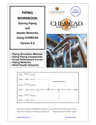
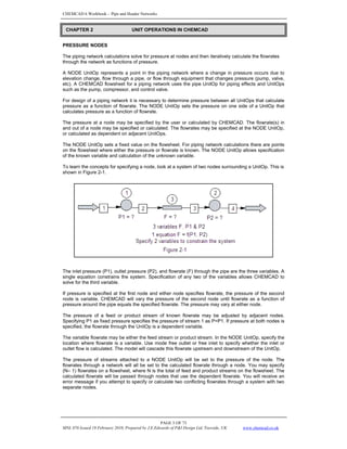
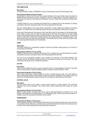
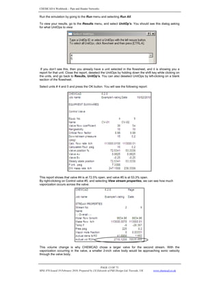
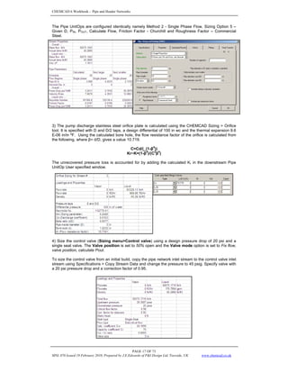
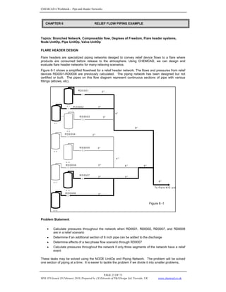
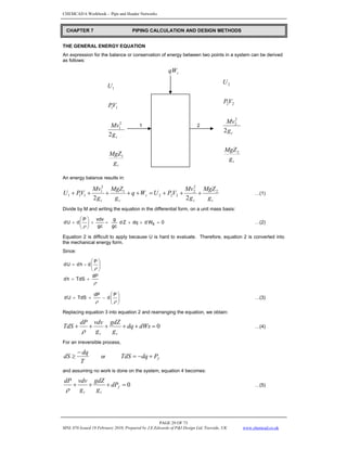
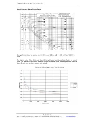
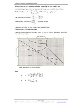
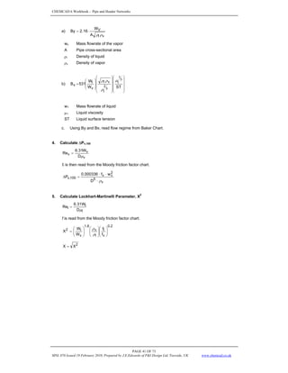
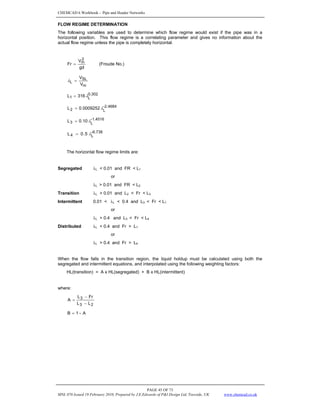
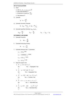
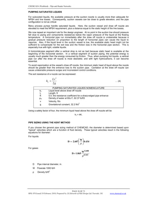
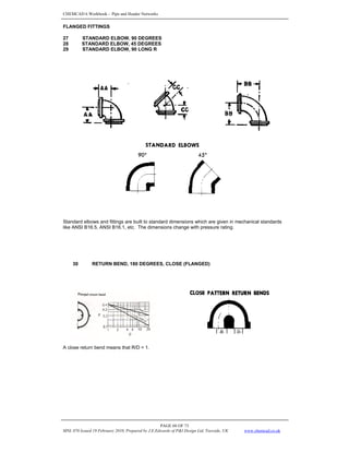
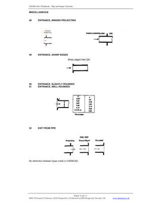
TWO-PHASE DENSITY
g
g
L
L
s H
H ρ
ρ
ρ +
=
)
0
(
)
0
( L
L H
H ϕ
=
HL (0) = The holdup which would exist at the same conditions in a horizontal pipe
HL (0) =
c
F
Lb
a
R
λ
For HL(0) > λL:
Flow Regime a b c
For segregated flow 0.98 0.4846 0.0868
For intermittent flow 0.845 0.5351 0.0173
For distributed flow 1.065 0.5824 0.0609
)
be
must
(H L
(o)
L λ
≥
The factor for correlating the holdup for the effect of pipe inclination is given by:
( ) ( )
[ ]
φ
−
φ
+
=
Ψ 8
.
1
sin
333
.
0
8
.
1
sin
C
1 3
θ = the actual angle of the pipe from horizontal
C =
( ) ( )
g
LV
L
L Fr
N
D f
e
λ
λ ln
1−
Flow Regime d e f g
For segregated uphill 0.011 -3.768 3.539 -1.614
For intermittent uphill 2.96 0.305 -0.4473 0.0978
For distributed uphill No correction c = 0, Ψ = 1, HL ≠ f (ø)
For all downhill 4.7 -0.3692 0.1244 -0.5056
with the restriction that C > 0.
FRICTION FACTOR
D
g
2
V
f
d
dP
c
2
m
n
tp
f •
•
•
=
⎟
⎟
⎠
⎞
⎜
⎜
⎝
⎛
Ζ
ρ
( )
L
g
L
g
g
L
L
n 1 λ
ρ
λ
ρ
λ
ρ
λ
ρ
ρ −
•
+
•
=
•
+
•
=
( )
L
g
L
L
g
g
L
L
n 1
m
m λ
λ
μ
λ
λ
μ
μ −
•
+
•
=
•
+
•
=
n
m
n
Ren
d
V
N
μ
ρ •
•
=
ftp = fn ∗ X where S
e
=
X
( ) ( )4
2
lny
01853
.
0
lny
0.8725
-
lny
3.182
0.0523
-
lny
s
•
+
•
•
+
=
( )
2
L
L
H
y
φ
λ
=
The value of y becomes unbounded at a point in the interval 1< y < 1.2; and for y in this interval, the
function S is calculated from:
S = ln( 2.2y – 1.2 )

47. CHEMCAD 6 Workbook - Pipe and Header Networks
PAGE 47 OF 73
MNL 076 Issued 19 February 2010, Prepared by J.E.Edwards of P&I Design Ltd, Teesside, UK www.chemcad.co.uk
ACCELERATION TERM
dZ
dP
E
dZ
dP
P
g
V
V
dZ
dP
k
c
sg
m
s
acc
•
=
•
•
•
•
=
⎟
⎠
⎞
⎜
⎝
⎛ ρ
Since acc
f
el dZ
dP
dZ
dP
dZ
dP
dZ
dP
⎟
⎠
⎞
⎜
⎝
⎛
+
⎟
⎠
⎞
⎜
⎝
⎛
+
⎟
⎠
⎞
⎜
⎝
⎛
=
⎟
⎠
⎞
⎜
⎝
⎛
⎟
⎠
⎞
⎜
⎝
⎛
•
+
⎟
⎠
⎞
⎜
⎝
⎛
+
⎟
⎠
⎞
⎜
⎝
⎛
=
⎟
⎠
⎞
⎜
⎝
⎛
dZ
dP
E
dZ
dP
dZ
dP
dZ
dP
k
f
el
f
el
k
dZ
dP
dZ
dP
dZ
dP
E
dZ
dP
⎟
⎠
⎞
⎜
⎝
⎛
+
⎟
⎠
⎞
⎜
⎝
⎛
=
•
−
k
f
el
E
-
1
dZ
dP
dZ
dP
dZ
dP
⎟
⎠
⎞
⎜
⎝
⎛
+
⎟
⎠
⎞
⎜
⎝
⎛
=
⎟
⎠
⎞
⎜
⎝
⎛
ELEVATION TERM
gc
g
d
dP s
el
•
=
⎟
⎠
⎞
⎜
⎝
⎛
Ζ
ρ
gc Gravitational constant
g Acceleration due to gravity

48. CHEMCAD 6 Workbook - Pipe and Header Networks
PAGE 48 OF 73
MNL 076 Issued 19 February 2010, Prepared by J.E.Edwards of P&I Design Ltd, Teesside, UK www.chemcad.co.uk
VERTICAL FLOW
For vertical flow, θ = 1, and dL = dZ, so;
acc
f
el dZ
dP
dZ
dP
dZ
dP
dZ
dP
dL
dP
⎟
⎠
⎞
⎜
⎝
⎛
+
⎟
⎠
⎞
⎜
⎝
⎛
+
⎟
⎠
⎞
⎜
⎝
⎛
=
=
The pressure drop caused by elevation change depends on the density of the two-phase mixture and is
usually calculated using a liquid holdup value. Except for high velocity situations, most of the pressure
drop in vertical flow is caused by elevation change. The frictional pressure loss requires evaluation of
the two-phase friction factor. The acceleration loss is usually ignored except for high velocity cases.
VERTICAL FLOW REGIMES
Bubble flow
In bubble flow the pipe is almost completely filled with liquid and the free gas phase is present in small
bubbles. The bubbles move at different velocities and except for their density, have little effect on the
pressure gradient. The wall of the pipe is always contacted by the liquid phase.
Slug flow
In slug flow the gas phase is more pronounced. Although the liquid phase is still continuous, the gas
bubbles coalesce and form plugs or slugs, which almost fill the pipe cross-section. The gas bubble
velocity is greater than that of the liquid. The liquid in the film around the bubble may move downward
at low velocities. Both the gas and liquid have significant effects on the pressure gradient.
Transition flow
The change from a continuous liquid phase to a continuous gas phase is called transition flow. The gas
bubbles may join and liquid may be entrained in the bubbles. Although the liquid effects are significant,
the gas phase effects are predominant.
Mist flow
In mist flow, the gas phase is continuous and the bulk of the liquid is entrained as droplets in the gas
phase. The pipe wall is coated with a liquid film, but the gas phase predominantly controls the pressure
gradient.
Illustrations of bubble, slug, transition, and mist flow are shown below.
Figure 7-5: Vertical Flow Patterns
A typical two-phase flow regime map is shown on Figure 7-6.

49. CHEMCAD 6 Workbook - Pipe and Header Networks
PAGE 49 OF 73
MNL 076 Issued 19 February 2010, Prepared by J.E.Edwards of P&I Design Ltd, Teesside, UK www.chemcad.co.uk
Where the following are the procedure equations for calculating vertical flow with Beggs and Bill method.
4
1
T
S
g
V
N L
SL
LV ⎟
⎟
⎠
⎞
⎜
⎜
⎝
⎛
=
ρ
4
1
T
S
g
V
N L
SV
GV ⎟
⎟
⎠
⎞
⎜
⎜
⎝
⎛
=
ρ
2
1
ST
g
d
N L
D ⎟
⎟
⎠
⎞
⎜
⎜
⎝
⎛
=
ρ
4
1
3
L
L
L
ST
g
N
⎟
⎟
⎠
⎞
⎜
⎜
⎝
⎛
=
ρ
μ
LV
N
36
50
LS +
=
0.75
LV
M N
84
75
L +
=
Figure 7-6: Flow Regime Map
NLv
Ngv

50. CHEMCAD 6 Workbook - Pipe and Header Networks
PAGE 50 OF 73
MNL 076 Issued 19 February 2010, Prepared by J.E.Edwards of P&I Design Ltd, Teesside, UK www.chemcad.co.uk
SET UP CALCULATIONS
1) Given
a. Inlet ST
,
,
,
,
,
m
,
m L
v
L
v
L
v μ
μ
ρ
ρ
b. Pipe inside diameter, D
c. Acceleration of gravity, g, 2
s
ft
d. Inlet pressure, P
2) Calculate
3)
4
D
A
2
π
=
4) Calculate Volumetric Flowrates
5)
L
L
L
v
v
g
m
Q
&
m
Q
ρ
ρ
=
=
6) Calculate Superficial Velocities m
sl
sg V
,
V
,
V
sl
sg
m
L
sl
g
sg V
V
V
A
Q
V
A
Q
V +
=
=
=
DETERMINE FLOW REGIME
5. Calculate Froude No.
7)
gD
v
R
F
2
m
=
6. Calculate No-slip liquid holdup
8)
m
sl
L
v
v
=
= λ
7. Calculate dimension less “L” parameters
302
.
0
L
1 316
L λ
=
4684
.
2
L
2 0009252
.
0
L −
= λ
4516
.
1
L
3 10
.
0
L −
= λ
738
.
6
L
4 5
.
0
L −
= λ
8. Apply flow regime rules
a. Is ?
L
r
F
and
01
.
0 1
L 〈
〈
λ
↓
→ flow
Segregated
Yes
No
b. Is ?
L
r
F
and
01
.
0 2
L 〈
≥
λ
↓
→ flow
Segregated
Yes
No
c. Is 3
2
L L
r
F
L
and
01
.
0 ≤
≤
≥
λ ?
↓
→ flow
Transition
Yes
No
d. Is 1
3
L L
r
F
L
and
4
.
0
01
.
0 ≤
〈
〈
≤ λ ?
↓
→ flow
nt
Intermitte
Yes
No
e. Is 4
3
L L
r
F
L
and
4
.
0 ≤
〈
≥
λ ?
↓
→ flow
nt
Intermitte
Yes
No

51. CHEMCAD 6 Workbook - Pipe and Header Networks
PAGE 51 OF 73
MNL 076 Issued 19 February 2010, Prepared by J.E.Edwards of P&I Design Ltd, Teesside, UK www.chemcad.co.uk
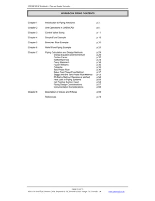
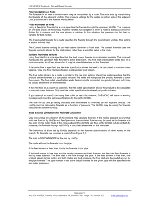
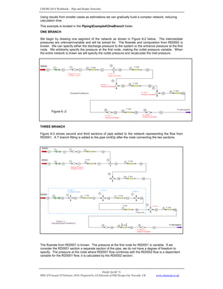
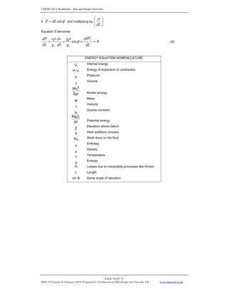
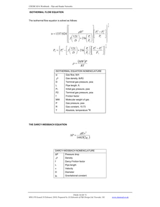
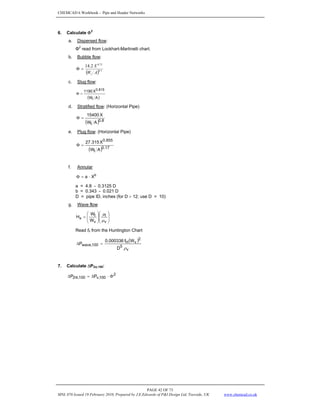
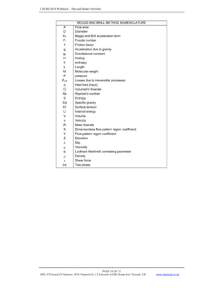
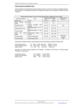
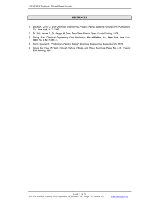
f. Is 1
L L
r
F
and
4
.
0 ≥
〈
λ ?
↓
→ flow
d
Distribute
Yes
No
g. Is 4
L L
r
F
and
4
.
0 〉
≥
λ ?
method
Brill
-
Beggs
the
of
range
the
Outside
flow
d
Distribute
Yes
No
↓
→
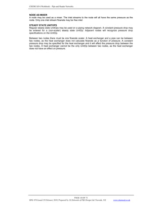
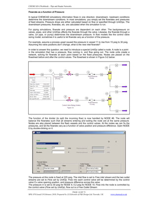
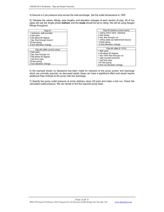
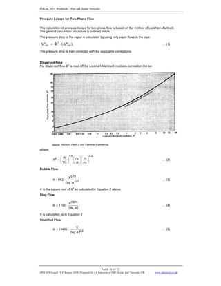
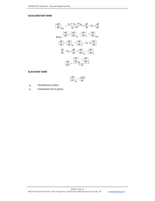
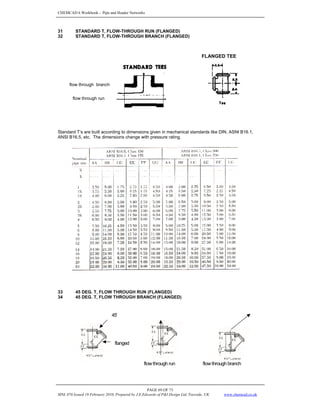
DETERMINE LIQUID HOLDUP & TWO-PHASE DENSITY
9. Calculate (o)
L
H (the holdup which would exist at the same conditions in a horizontal pipe.)
c
r
b
L
(o)
2
F
a
H
λ
=
Flow Regime a b c
For segregated flow 0.98 0.4846 0.0868
For intermittent flow 0.845 0.5351 0.0173
For distributed flow 1.065 0.5824 0.0609
)
be
must
(H L
(o)
L λ
≥
For transition flow calculate HL (segregated) and HL (Intermittent).
10. Calculate LV
N (the liquid velocity number)
4
1
L
sl
LV
T
S
g
V
N ⎟
⎟
⎠
⎞
⎜
⎜
⎝
⎛
=
ρ
11. Calculate c
( ) ⎟
⎠
⎞
⎜
⎝
⎛ •
•
•
•
−
= g
r
f
LV
e
L
1
L F
N
D
ln
1
c λ
λ
Flow Regime D1
e f g
For segregated uphill 0.011 -3.768 3.539 -1.614
For intermittent uphill 2.96 0.305 -0.4473 0.0978
For distributed uphill No correction c = 0, Ψ = 1, HL ≠ f (ø)
For all downhill 4.7 -0.3692 0.1244 -0.5056
For transition uphill flow, calculate c (segregated) and c (intermittent). (C must be ≥ 0)
12. Calculate Ψ
Ψ = 1 + c [ sin (1.8 ø) – 0.333 sin
3
(1.8 ø)]
where φ is the actual angle of the pipe from horizontal. For vertical flow ø = 90.
13. Calculate the liquid holdup, HL (ø)
For segregated, intermittent, and distributed flow:
Ψ
⋅
= (0)
L
(ø)
L H
H
For transition flow:
HL (transition) = A • HL (segregated) + B • HL (intermittent)
2
3
r
3
L
L
F
L
A
−
−
=
A
-
1
B =
14. Calculate Hg = 1 – HL (ø)
15. Calculate two phase density g
g
(ø)
L
L
s H
H ⋅
+
⋅
= ρ
ρ
ρ

52. CHEMCAD 6 Workbook - Pipe and Header Networks
PAGE 52 OF 73
MNL 076 Issued 19 February 2010, Prepared by J.E.Edwards of P&I Design Ltd, Teesside, UK www.chemcad.co.uk
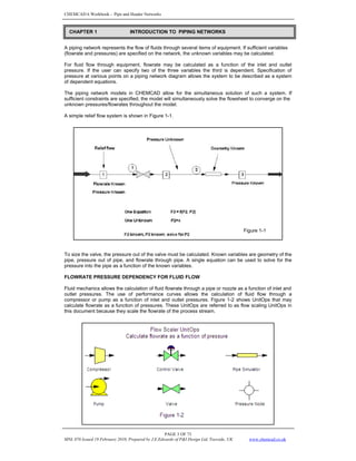
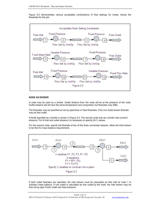
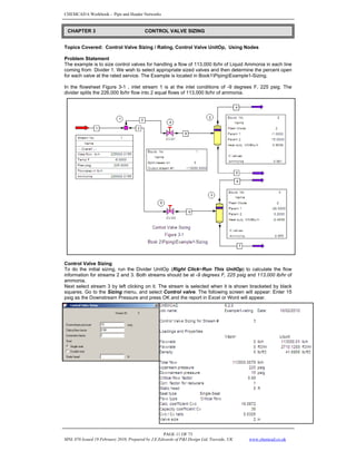
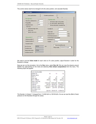
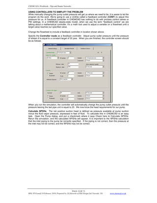
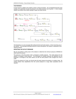
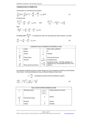
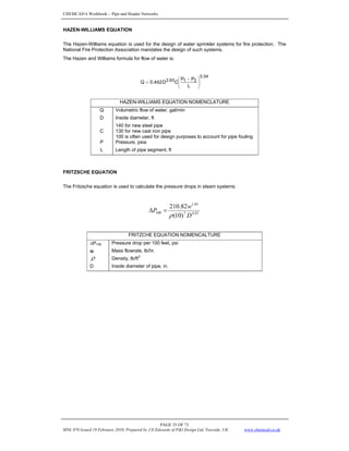
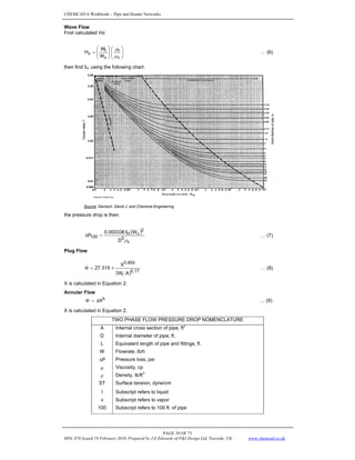
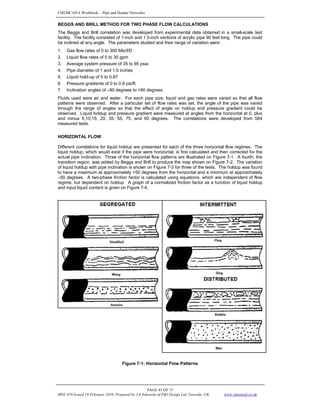
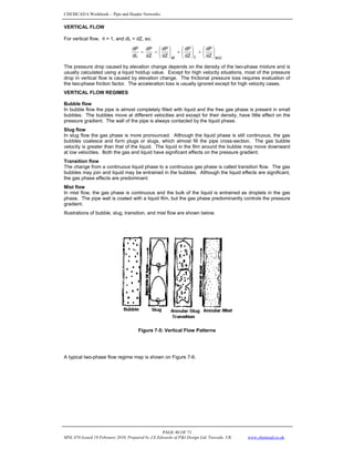
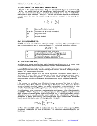
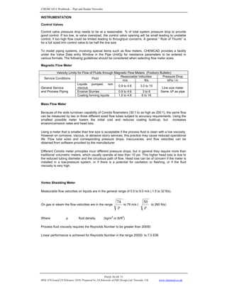
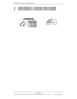
DETERMINE ELEVATION TERM
[ ] ft.
psf
dZ
dP
el
=
⎟
⎠
⎞
⎜
⎝
⎛
16.
gc
g
d
dP s
el
•
=
⎟
⎠
⎞
⎜
⎝
⎛
Ζ
ρ
DETERMINE FRICTION TERM
f
d
dP
⎟
⎠
⎞
⎜
⎝
⎛
Ζ
17. Calculate no-slip two-phase density
( )
L
g
L
g
g
L
L
n 1 λ
ρ
λ
ρ
λ
ρ
λ
ρ
ρ −
•
+
•
=
•
+
•
=
18. Calculate no-slip viscosity, μn
( )
L
g
L
L
g
g
L
L
n 1
m
m λ
λ
μ
λ
λ
μ
μ −
•
+
•
=
•
+
•
=
19. Calculate no-slip Reynold’s No.
n
m
n d
V
Re
μ
ρ •
•
=
20. Calculate no-slip friction factor
( )
2
n
8215
.
3
Re
log
4.5223
Re
log
2
1
f
⎥
⎦
⎤
⎢
⎣
⎡
⎟
⎠
⎞
⎜
⎝
⎛
−
•
•
=
21. Calculate
9)
( )
2
L
L
H
y
⎟
⎠
⎞
⎜
⎝
⎛
=
φ
λ
22. Calculate
( ) ( )4
2
lny
01853
.
0
ln(y)
0.8725
-
lny
3.182
0.0523
-
ln(y)
s
•
+
•
•
+
=
23. Calculate the two phase friction factor
s
n
tp e
f
f •
=
24. Calculate the friction loss term,
f
d
dP
⎟
⎠
⎞
⎜
⎝
⎛
Ζ
d
2
v
f
d
dP
gc
2
m
n
tp
f •
•
•
=
⎟
⎟
⎠
⎞
⎜
⎜
⎝
⎛
Ζ
ρ
CALCULATE THE ACCELERATION TERM
25.
P
gc
v
v
E
sg
m
s
k
•
•
•
=
ρ
CALCULATE THE TOTAL PRESSURE GRADIENT
⎟
⎠
⎞
⎜
⎝
⎛
Ζ
d
dP
26.
k
el
f
E
-
1
d
dP
d
dP
d
dP
⎟
⎠
⎞
⎜
⎝
⎛
Ζ
+
⎟
⎠
⎞
⎜
⎝
⎛
Ζ
=
Ζ

53. CHEMCAD 6 Workbook - Pipe and Header Networks
PAGE 53 OF 73
MNL 076 Issued 19 February 2010, Prepared by J.E.Edwards of P&I Design Ltd, Teesside, UK www.chemcad.co.uk
BEGGS AND BRILL METHOD NOMENCLATURE
A Flow area
D Diameter
Ek Beggs and Brill acceleration term
Fr Froude number
f Friction factor
g Acceleration due to gravity
gc Gravitational constant
H Holdup
h enthalpy
L Length
M Molecular weight
P pressure
PLW Losses due to irreversible processes
q Heat loss (input)
Q Volumetric flowrate
Re Reynold’s number
S Entropy
SG Specific gravity
ST Surface tension
U Internal energy
V Volume
v Velocity
W Mass flowrate
X Dimensionless flow pattern region coefficient
Y Flow pattern region coefficient
Z Elevation
λ Slip
μ Viscosity
Φ Lockhart–Martinelli correlating parameter
ρ Density
τ Shear force
2Φ Two phase

54. CHEMCAD 6 Workbook - Pipe and Header Networks
PAGE 54 OF 73
MNL 076 Issued 19 February 2010, Prepared by J.E.Edwards of P&I Design Ltd, Teesside, UK www.chemcad.co.uk
3-K (DARBY) METHOD OF SPECIFYING FLOW RESISTANCES
In the past, the flow resistance of values and fittings has been represented by one or two numbers; L/D,
K, Kf, etc. This method is accurate over a wide range of Reynolds numbers, but does not accurately
reflect data over a wide range of sizes. Specifically, these methods tend to under predict the friction
loss for pipes of larger diameters. Darby (2001) evaluated data from the literature for various valves,
tees, and elbows and found that they can be represented more accurately by the following “3-K”
equation:
⎟
⎟
⎠
⎞
⎜
⎜
⎝
⎛
+
+
=
0.3
n
d
i
1
f
D
K
1
K
Re
K
K
Kf Loss coefficient, dimensionless
K1, Ki, Kd Constants, can be found in the literature
Re Reynolds number
Dn Nominal diameter
HEAT LOSS IN PIPING SYSTEMS
The PIPE module will calculate the heat lost (or gained) to the surroundings if the user enters the overall
heat transfer coefficient, U, and the ambient temperature, Ta. The heat loss is calculated as follows:
)
( b
a T
T
UA
Q −
=
Q The heat transferred to the surroundings
(negative indicator heat lost from the piping system).
U The overall heat transfer coefficient (user specified).
Ta The ambient temperature (user specified).
Tb The temperature of the bulk material in the pipe.
NET POSITIVE SUCTION HEAD
Centrifugal pumps require vapor free liquid flow in the suction line at the entrance to the impeller vanes
to operate satisfactorily. Reciprocating pumps require such flow right after the inlet valve.
A centrifugal pump cannot pump vapor-liquid mixtures. A positive-displacement pump can pump liquids
containing vapor but its volumetric efficiency will be greatly reduced, even if the weight percentage of
vapor is a very small proportion of total flow.
The pressure gradient along the liquid path through a pump has characteristics similar to those of a
control valve or orifice. Instead of a pressure loss, however, the downstream pressure will become
much greater than the suction pressure. In both the pump-suction land the pump discharge, the
minimum pressure should not drop below the vapor pressure of the liquid at the flowing temperature.
NPSHr
If the pressure in a centrifugal pump falls below the vapor pressure of the liquid at the flowing
temperature, bubbles form just before the inlet edge of the impeller vanes. Because of the rapid
increase in pressure within the impeller, the bubbles then collapse. This phenomenon is called
cavitation. It can reduce pump efficiency and cause noise, vibration, impeller wear and damage.
To avoid cavitation, pump manufacturers require a positive suction pressure called net positive suction
head, NPSHr . NPSHr is the pressure above the vapor pressure of the liquid being pumped, measured
as the pump-suction flange on a gage at the pump centerline. It is the pressure necessary to overcome
friction and turbulence losses between the suction nozzle and the entrance to the impeller, and is
usually given as head of water on pumps’ head-capacity curves. NPSHr, for a pump will increase with
flowrate, and considerably increases with rotating speed of the impeller:
( )1
r
2
2
r NPSH
1
2
)
NSPH
(
n
n
⎟
⎟
⎠
⎞
⎜
⎜
⎝
⎛
= … (1)
For flows below about 20 to 25% of rated capacity (near the maximum efficiency points), NPSHr
requirements can be higher than those for normal flow. This is especially true with high-capacity, low-
head pumps.

55. CHEMCAD 6 Workbook - Pipe and Header Networks
PAGE 55 OF 73
MNL 076 Issued 19 February 2010, Prepared by J.E.Edwards of P&I Design Ltd, Teesside, UK www.chemcad.co.uk
NPSHa
Available net positive suction head, NPSHa , is the potential energy of an installation, expressed in feet
of liquid head, and can be calculated from:
( )
144
ρ
a
NPSH
P = … (2)
If we let,
( ) w
SG ρ
ρ =
Equation 2 becomes:
( )
SG
P
NPSHa 31
.
2
= … (3)
NET POSITION SUCTION HEAD NOMENCLATURE
( )2
r
NSPH The required net positive suction head if pump speed is increased to n2
rpm
( )1
r
NSPH Obtained from the pump’s head-capacity curve
n1 Obtained from the pump’s head-capacity curve
n2
P Pressure above vapor pressure at the centerline of the suction flange,
psia.
( )
a
NSPH Available net positive suction head
ρ Density of fluid at flowing temperature, lb/ft
3
SG Specific gravity of liquid at flowing temperature
ρw Density of water at 60o F, 62.37 lb/ft3
To ensure reliable pump operation, NPSHa should equal or exceed NPSHr. Thus, process equipment
must be elevated at least as high as the sum of the pump’s NPSHr, plus the friction-head losses in the
suction line when saturated liquids are pumped.
At the suction nozzle, velocity head is also a positive energy component. However, this is not included
in NPSH diagrams for pumps made in the U.S. Consequently, in calculations for NPSHa, velocity head
does not have to be considered.
According to the Hydraulic Institute “The NPSH requirements of centrifugal pumps are normally
determined on the basis of handling water. It is recognized that when pumping hydrocarbons, the
NPSHr required to obtain satisfactory operation may be reduced for certain conditions. However, it is
customary to use manufacturers’ data for the minimum required NPSHr when handling hydrocarbons
having specific gravities less than 1. This means that:
1. Both available and required NPSHr do not vary with the liquid’s specific gravity.
2. For a given centrifugal pump, one curve of required NPSHr can be used with all normal
specific gravities.
The effect of specific gravity can be explained as follows: Looking at the analogy of NPSH as a force
that pushes liquid into a pump, and assuming a pump that has an NPSHr of 8 ft. at a given capacity, we
can show that a head of 8 ft. of water equals 3.45 psi, while a head of 8 ft. of gasoline equals 2.60 psi. It
would appear that the force pushing liquid into the pump decreases with specific gravity. However, the
mass of liquid being accelerated has decreased by the same proportion.
When choosing between two pumps of equal capacity, the one having the higher NPSHr will cost less.
But the less-expensive pump will be the economic choice only if its cost advantage is not offset by the
expense of elevating the process equipment. Often, a vertical pump will be specified to bring equipment
closer to grade elevation.
If a reciprocating pump is to transfer saturated liquid and if we desire maximum volumetric efficiency, we
make analyses and calculations for NPSH conditions similar to those for centrifugal pumps. Resistance
at the inlet valve of a reciprocating pump is greater than the entrance loss to an impeller. Due to
pulsating liquid flow, we must also take into account increased line resistance.

56. CHEMCAD 6 Workbook - Pipe and Header Networks
PAGE 56 OF 73
MNL 076 Issued 19 February 2010, Prepared by J.E.Edwards of P&I Design Ltd, Teesside, UK www.chemcad.co.uk
PUMPING SATURATED LIQUIDS
For subcooled liquids, the available pressure at the suction nozzle is usually more than adequate for
NPSH and line losses. Consequently, suction vessels can be close to grade elevation, and the pipe
configuration is not as critical.
Many process pumps handle saturated liquids. Here, the suction vessel and draw off nozzle are
elevated to meet the NPSH requirement, plus a distance equal to the static height of the line losses.
We now repeat an important rule for the design engineer. At no point in the suction line should pressure
fall (due to piping and components resistance) below the vapor pressure of the liquid at the flowing
temperature. A horizontal pipe run immediately after the draw off nozzle is undesirable because a
gradual pressure reduction (in proportion to the length of horizontal pipe) can cause the liquid to
vaporize. Also, if the liquid level in the suction vessel is low, the available static head might not be
sufficient to compensate for the exit loss and the friction loss in the horizontal pipe section. This is
especially true with light, volatile liquids.
A horizontal-pipe segment after a vertical drop is not as bad because static head is available at the
beginning of the horizontal section. In a vertical segment of suction piping, the potential energy is
usually much greater than the energy consumed by friction. Thus, when pumping hot liquids, a vertical
pipe run after the draw off nozzle is most desirable; and with light hydrocarbons, it can become
essential.
To avoid vaporization at the vessel’s draw off nozzle, the minimum static head of liquid above the nozzle
should be greater than the entrance loss to the suction pipe. Cavitation at the draw off nozzle can
cause undesirable pressure surges and inconsistent control conditions.
The exit resistance of a nozzle can be expressed:
g
Lv
hL
2
2
= … (4)
PUMPING SATURATED LIQUIDS NOMENCLATURE
hL Liquid level above draw off nozzle
L Length, ft
K 0.5, the resistance coefficient for a sharp-edged pipe entrance
ρw Density of water at 60o F, 62.37 lb/ft3
v Velocity, ft/s
g Gravitational constant, 32.2 ft/s
2
Using a safety factor of four, the minimum liquid head above the draw off nozzle will be
hL = 4K.
PIPE SIZING USING THE KENT METHOD
If you choose the general pipe sizing method of CHEMCAD, the diameter is determined based upon
“typical” velocities which are a function of fluid density. These typical velocities result in the following
equations for diameter:
For liquids:
434
.
0
W
2.607
D ⎟
⎟
⎠
⎞
⎜
⎜
⎝
⎛
ρ
=
For gases:
343
.
0
408
.
0
W
065
.
1
D
ρ
=
D Pipe internal diameter, in.
W Flowrate 1000 lb/h
ρ Density lb/ft3

57. CHEMCAD 6 Workbook - Pipe and Header Networks
PAGE 57 OF 73
MNL 076 Issued 19 February 2010, Prepared by J.E.Edwards of P&I Design Ltd, Teesside, UK www.chemcad.co.uk
PIPING DESIGN CONSIDERATIONS
Industry practice for initial design of piping systems is based on economic velocity or allowable pressure
drop ∆P/100ft. Once detailed isometrics are available the design will be adjusted to satisfy local site
conditions.
Reasonable Velocities for Flow of Fluids through Pipes (Reference Crane 410M)
Reasonable Velocities Pressure Drop
Service Conditions Fluid
m/s ft/s kPa / m
Boiler Feed Water 2.4 to 4.6 8 to 15
Pump Suction and
Drain
Water 1.2 to 2.1 4 to 7
General Service
Liquids pumped, non
viscous
1.0 to 3.0 3.2 to 10 0.05
Heating Short Lines
Saturated Steam 0 to 1.7
bar
20 to 30 65 to 100
Process piping
Saturated Steam 1.7 and
up
30 to 60 100 to 200
Boiler and turbine
leads
Superheated Steam 14
and up
30 to 100 100 to 325
Process piping Gases and Vapours 15 to 30 50 to 100
0.02% line
pressure
Process piping Liquids gravity flow 0.05
Reasonable velocities based on pipe diameter (Process Plant Design, Backhurst Harker p235)
Pump suction line for d in (d/6 + 1.3) ft/s and d mm (d/500 + 0.4) m/s
Pump discharge line for d in (d/3 + 5) ft/s and d mm (d/250 + 1.5) m/s
Steam or gas d in 20d ft/s and d mm 0.24d m/s
Heuristics for process design (Reference W.D.Seader, J.D.Seider and D.R.Lewin, “Process Design
Principles”) are also given:
Liquid Pump suction (1.3 + d/6) ft/s 0.4 psi /100 ft
Liquid Pump discharge (5.0 + d/3) ft/s 2.0 psi / 100 ft
Steam or gas (20d) ft/s 0.5 psi / 100 ft

58. CHEMCAD 6 Workbook - Pipe and Header Networks
PAGE 58 OF 73
MNL 076 Issued 19 February 2010, Prepared by J.E.Edwards of P&I Design Ltd, Teesside, UK www.chemcad.co.uk
INSTRUMENTATION
Control Valves
Control valve pressure drop needs to be at a reasonable % of total system pressure drop to provide
good control. If too low, ie valve oversized, the control valve opening will be small leading to unstable
control; if too high flow could be limited leading to throughput concerns. A general “ Rule of Thumb” is
for a full sized trim control valve to be half the line size.
To model piping systems, involving special items such as flow meters, CHEMCAD provides a facility
under the Valve Data entry Window in the Pipe UnitOp for resistance parameters to be entered in
various formats. The following guidelines should be considered when selecting flow meter sizes.
Magnetic Flow Meter
Velocity Limits for Flow of Fluids through Magnetic Flow Meters (Foxboro Bulletin)
Reasonable Velocities Pressure Drop
Service Conditions Fluid
m/s ft/s kPa / m
Liquids pumped, non
viscous
0.9 to 4.6 3.0 to 15
Erosive Slurries 0.9 to 4.6 3 to 6
General Service
and Process Piping
Coating forming liquids 1.8 to 4.6 6 to 16
Line size meter
Same ∆P as pipe
Mass Flow Meter
Because of the wide turndown capability of Coriolis flowmeters (30:1 to as high as 200:1), the same flow
can be measured by two or three different sized flow tubes subject to accuracy requirements. Using the
smallest possible meter lowers the initial cost and reduces coating build-up, but increases
erosion/corrosion rates and head loss.
Using a meter that is smaller than line size is acceptable if the process fluid is clean with a low viscosity.
However on corrosive, viscous, or abrasive slurry services, this practice may cause reduced operational
life. Flow tube sizes and corresponding pressure drops, inaccuracies, and flow velocities can be
obtained from software provided by the manufacturer.
Different Coriolis meter principles incur different pressure drops, but in general they require more than
traditional volumetric meters, which usually operate at less than 10 psi. This higher head loss is due to
the reduced tubing diameter and the circuitous path of flow. Head loss can be of concern if the meter is
installed in a low-pressure system, or if there is a potential for cavitation or flashing, or if the fluid
viscosity is very high.
Vortex Shedding Meter
Measurable flow velocities on liquids are in the general range of 0.5 to 9.0 m/s ( 1.5 to 32 ft/s).
On gas or steam the flow velocities are in the range
ρ
74
to 79 m/s (
ρ
50
to 260 ft/s)
Where ρ fluid density (kg/m
3
or lb/ft
3
)
Process fluid viscosity requires the Reynolds Number to be greater than 20000
Linear performance is achieved for Reynolds Number in the range 20000 to 7.0 E06

59. CHEMCAD 6 Workbook - Pipe and Header Networks
PAGE 59 OF 73
MNL 076 Issued 19 February 2010, Prepared by J.E.Edwards of P&I Design Ltd, Teesside, UK www.chemcad.co.uk
VALVES FLANGED FITTINGS
1 Gate valve 27 Standard elbow 90 deg
2 Globe seat flat, bevel, plug 28 Standard elbow 45 deg
3 Globe wing/pin guided disk 29 Standard elbow 90 long R
4 Angle, no obstruction 30 Return bend 180 deg close
5 Angle wing/pin guided disc 31 Standard T, flow-through run
6 Y-pattern globe 60 deg 32 Standard T, flow-through branch
7 Y-pattern globe 45 deg 33 45 deg T, flow-through run
8 Ball valve 34 45 deg T, flow-through branch
9 Butterfly 2-8 inches 35 Elbow 90 deg, R/D = 1.0
10 Butterfly 10-14 inches 36 Elbow 90 deg, R/D = 1.5
11 Butterfly 14-24 inches 37 Elbow 90 deg, R/D = 2.0
12 Plug, straight-way WELDED FITTINGS
13 Plug, 3-way (straight way) 38 Elbow 45 deg, R/D = 1.0
14 Plug, 3-way through branch 39 Elbow 45 deg, R/D = 1.5
15 Foot valve, poppet disk 40 Elbow 45 deg, R/D = 2.0
16 Foot valve, hinged disk 41 Return bend 180, R/D = 1.0
17 Swing check, clearway 42 Return bend 180, R/D = 1.5
18 Swing check, tilting seat 43 Return bend 180, R/D = 2.0
19 Tilt disk 5 deg 2-8 in 44 Tee 100% flow-through run
20 Tilt disk 5 deg 10-14 in 45 Tee 100% flow-out branch
21 Tilt disk 5 deg 16-48 in 46 Tee 100% flow-in branch
22 Tilt disk 15 deg 2-8 in 47 Reducer
23 Tilt disk 15 deg 10-14 in MISCELLANEOUS
24 Tilt disk 15 deg 16-48 in 48 Entrance, inward project
25 Lift of stop check, globe 49 Entrance, sharp edged
26 Lift or stop check, angle 50 Entrance, slightly round
51 Entrance, well rounded
52 Exit from pipe
53 Sudden contraction (DSMALL/DLARGE)
54 Sudden expansion (DSMALL/DLARGE)
CHAPTER 8 DESCRIPTION OF VALVES AND FITTINGS

60. CHEMCAD 6 Workbook - Pipe and Header Networks
PAGE 60 OF 73
MNL 076 Issued 19 February 2010, Prepared by J.E.Edwards of P&I Design Ltd, Teesside, UK www.chemcad.co.uk
VALVE DIAGRAMS
1 GATE VALVE
Wedge disc Double disc Plug Type

61. CHEMCAD 6 Workbook - Pipe and Header Networks
PAGE 61 OF 73
MNL 076 Issued 19 February 2010, Prepared by J.E.Edwards of P&I Design Ltd, Teesside, UK www.chemcad.co.uk
2 GLOBE VALVE, BEVEL, PLUG
Globe valve with seat that receives flat, beveled, or plug type disks. All three of these are welded the
same.
a. Seat arrangement diagrams

62. CHEMCAD 6 Workbook - Pipe and Header Networks
PAGE 62 OF 73
MNL 076 Issued 19 February 2010, Prepared by J.E.Edwards of P&I Design Ltd, Teesside, UK www.chemcad.co.uk
3 GLOBE VALVE WING/PIN GUIDED DISK
Globe valve with disk guided by pin or wing.
Pin guided disk
4 ANGLE, NO OBSTRUCTION
Angle valve with no obstruction; that is, no disk guides.
Angle valves are basically globe valves having inlet and outlet connections at right angles.
The overall construction elements of an angle valve are basically the same for the stern, disk
and seat-rings design as the globe valve.
Disk
Pin guide
General diagram of angle valves

63. CHEMCAD 6 Workbook - Pipe and Header Networks
PAGE 63 OF 73
MNL 076 Issued 19 February 2010, Prepared by J.E.Edwards of P&I Design Ltd, Teesside, UK www.chemcad.co.uk
5 ANGLE, WING/PIN GUIDED DISK
Angle valve with wing or pin disk guides(not shown)
6 Y-PATTERN GLOBE 60 DEGREES
7 Y-PATTERN GLOBE 45 DEGREES

64. CHEMCAD 6 Workbook - Pipe and Header Networks
PAGE 64 OF 73
MNL 076 Issued 19 February 2010, Prepared by J.E.Edwards of P&I Design Ltd, Teesside, UK www.chemcad.co.uk
8 BALL VALVE
General Diagram
The conventional ball valve, as the name implies, has a spherical plug that controls fluid flow. The two
basic types are the rotary motion ball valve and the lift or ball-in-cage type. The ball valve provides not
only tight shutoff but also good flow characteristics approaching those of an equal percentage valve.
For this reason, it is often applied as a combination throttling and shutoff valve. Due to low friction
forces, ball valves have been known to open gradually after prolonged exposure to vibration.
The most common body form is the two-way globe body. The spherical plug has a passage that aligns
with body parts in the open position. A quarter turn of the plug closes the valve. To achieve tight
shutoff, resilient seat rings are embedded in the body. Ball valves can be provided with three or four-
way plugs. In some installations this can represent a considerable savings in fittings, valves and space
since one unit can replace two or three flow through valves.
9 BUTTERFLY, 2-8 IN
10 BUTTERFLY, 10-14 IN
11 BUTTERFLY, 14-24 IN
Full bore valve shown
Reduced bore more common
Wafer valve shown
Direct lever operator shown
Flanged valve shown
Geared operator

65. CHEMCAD 6 Workbook - Pipe and Header Networks
PAGE 65 OF 73
MNL 076 Issued 19 February 2010, Prepared by J.E.Edwards of P&I Design Ltd, Teesside, UK www.chemcad.co.uk
12 PLUG, STRAIGHT WAY
13 PLUG, 3-WAY (STRAIGHT RUN)
14 PLUG, 3-WAY (THROUGH BRANCH)
15 FOOT VALVE, POPPET DISK
16 FOOT VALVE, HINGED DISK
Poppet Disc Hinged Disc
Straight Way
Straight Run Through Branch

66. CHEMCAD 6 Workbook - Pipe and Header Networks
PAGE 66 OF 73
MNL 076 Issued 19 February 2010, Prepared by J.E.Edwards of P&I Design Ltd, Teesside, UK www.chemcad.co.uk
17 SWING CHECK, CLEARWAY
18 SWING CHECK, TILTING SEAT
Also known as NON-RETURN VALVE
19 TILT DISK, 5 DEGREES 2-8 IN
20 TILT DISK, 5-DEGREES 10-14 IN
21 TILT DISK, 5 DEGREES 16-48 IN
22 TILT DISK, 15 DEGREES 2-8 IN
23 TILT DISK, 15 DEGREES 10-14 IN
24 TILT DISK, 15 DEGREES 16-48 IN
Also known as NON-RETURN VALVE

67. CHEMCAD 6 Workbook - Pipe and Header Networks
PAGE 67 OF 73
MNL 076 Issued 19 February 2010, Prepared by J.E.Edwards of P&I Design Ltd, Teesside, UK www.chemcad.co.uk
25 LIFT OR STOP CHECK VALVE, GLOBE
26 LIFT OR STOP CHECK VALVES, ANGLE
Stop-check valves are usually produced in globe or angle styles, with a stem that is used either to tightly
seat or to restrict the lift of the disk. The stem is not attached to the disk, and cannot be used to open
the valve. The stop-check valve is used on steam lines from boilers more than in any other application.
Foot valves are specialty check valves used at the bottom of a suction line on a horizontal pump. They
maintain the prime on such pumps and usually incorporate strainers to keep foreign matter from
entering.
Lift check valves, usually of the globe body form, depend on gravity for operation. They are designed
for either horizontal or vertical installation, but the two designs are not interchangeable. Under forward
flow, a piston is lifted off the seat by fluid while being retained in the valve by guides. On reverse flow,
the piston is forced against the seat to block further flow. Some lift check valves utilize spring loading to
assure positive seating. In any case, lift check valves require relatively high pressure drops. They are
used on higher pressure services and in smaller pipe sizes than swing checks.
Stop check valves, globe
type
Lift check valves,
globe type

68. CHEMCAD 6 Workbook - Pipe and Header Networks
PAGE 68 OF 73
MNL 076 Issued 19 February 2010, Prepared by J.E.Edwards of P&I Design Ltd, Teesside, UK www.chemcad.co.uk
FLANGED FITTINGS
27 STANDARD ELBOW, 90 DEGREES
28 STANDARD ELBOW, 45 DEGREES
29 STANDARD ELBOW, 90 LONG R
Standard elbows and fittings are built to standard dimensions which are given in mechanical standards
like ANSI B16.5, ANSI B16.1, etc. The dimensions change with pressure rating.
30 RETURN BEND, 180 DEGREES, CLOSE (FLANGED)
A close return bend means that R/D = 1.

69. CHEMCAD 6 Workbook - Pipe and Header Networks
PAGE 69 OF 73
MNL 076 Issued 19 February 2010, Prepared by J.E.Edwards of P&I Design Ltd, Teesside, UK www.chemcad.co.uk
31 STANDARD T, FLOW-THROUGH RUN (FLANGED)
32 STANDARD T, FLOW-THROUGH BRANCH (FLANGED)
Standard T’s are built according to dimensions given in mechanical standards like DIN, ASNI B16.1,
ANSI B16.5, etc. The dimensions change with pressure rating.
33 45 DEG. T, FLOW THROUGH RUN (FLANGED)
34 45 DEG. T, FLOW THROUGH BRANCH (FLANGED)
45
o
flanged
flowthrough run flowthrough branch
flow through branch
flow through run
FLANGED TEE

70. CHEMCAD 6 Workbook - Pipe and Header Networks
PAGE 70 OF 73
MNL 076 Issued 19 February 2010, Prepared by J.E.Edwards of P&I Design Ltd, Teesside, UK www.chemcad.co.uk
35. ELBOW 90 DEGREES, R/D = 1.0 (FOR WELDED, FLANGED, OR SCREWED)
36. ELBOW 90 DEGREES, R/D = 1.5 (FOR WELDED, FLANGED, OR SCREWED)
37. ELBOW 90 DEGREES, R/D = 2.0 (FOR WELDED, FLANGED, OR SCREWED)

71. CHEMCAD 6 Workbook - Pipe and Header Networks
PAGE 71 OF 73
MNL 076 Issued 19 February 2010, Prepared by J.E.Edwards of P&I Design Ltd, Teesside, UK www.chemcad.co.uk
WELDED FITTINGS
38 ELBOW 45 DEGREES, R/D = 1.0 (WELDED)
39 ELBOW 45 DEGREES, R/D = 1.5 (WELDED)
40 ELBOW 45 DEGREES, R/D = 2.0 (WELDED)
41 RETURN BEND 180, R/D = 1.0 (WELDED)
42 RETURN BEND 180, R/D = 1.5 (WELDED)
43 RETURN BEND 180, R/D = 2.0 (WELDED)
44 TEE 100% FLOW THROUGH RUN (WELDED)
45 TEE 100% FLOW OUT BRANCH (WELDED)
46 TEE 100% FLOW IN BRANCH (WELDED)
47. REDUCER CONCENTRIC OR ECCENTRIC (WELDED)

72. CHEMCAD 6 Workbook - Pipe and Header Networks
PAGE 72 OF 73
MNL 076 Issued 19 February 2010, Prepared by J.E.Edwards of P&I Design Ltd, Teesside, UK www.chemcad.co.uk
MISCELLANEOUS
48 ENTRANCE, INWARD PROJECTING
49 ENTRANCE, SHARP EDGED
50 ENTRANCE, SLIGHTLY ROUNDED
51 ENTRANCE, WELL ROUNDED
52 EXIT FROM PIPE
No distinction between types made in CHEMCAD.
Sharp edged inlet (24)

73. CHEMCAD 6 Workbook - Pipe and Header Networks
PAGE 73 OF 73
MNL 076 Issued 19 February 2010, Prepared by J.E.Edwards of P&I Design Ltd, Teesside, UK www.chemcad.co.uk
REFERENCES
1. Deutsch, David J. and Chemical Engineering; Process Piping Systems; McGraw-Hill Publications
Co.; New York, N. Y.,1980.
2. Dr. Brill, James P., Dr. Beggs, H. Dale; Two-Phase Flow in Pipes; Fourth Printing, 1978.
3. Darby, Ron; Chemical Engineering Fluid Mechanics; Marcel-Dekker, Inc.; New York, New York;
ISBN No. 0-8247-0444-4.
4. Kent , George R.; “Preliminary Pipeline Sizing” ; Chemical Engineering; September 25, 1978.
5. Crane Co; Flow of Fluids Through Valves, Fittings, and Pipes; Technical Paper No. 410; Twenty
Fifth Printing, 1991.