Physical and Logical Clocks

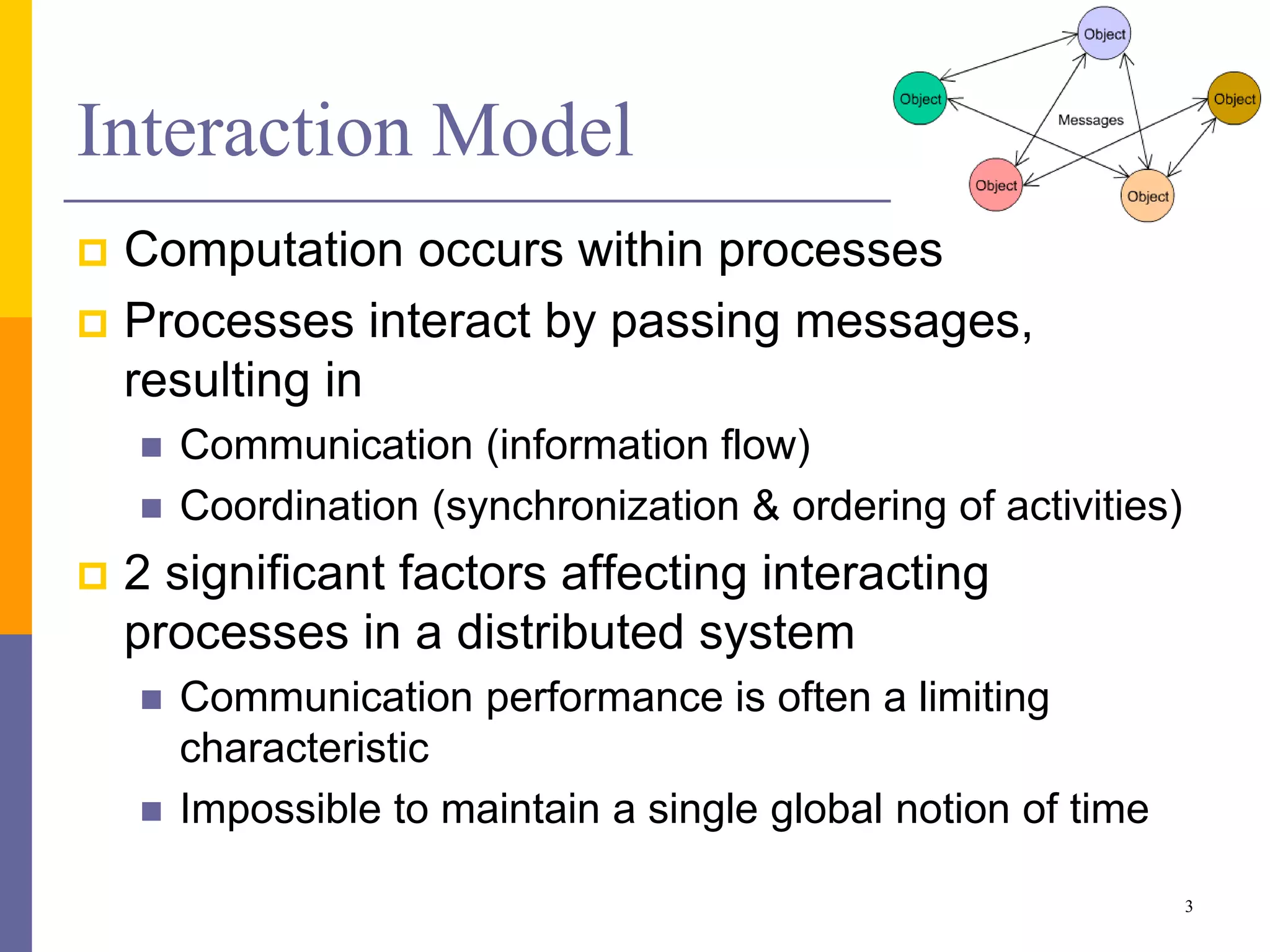
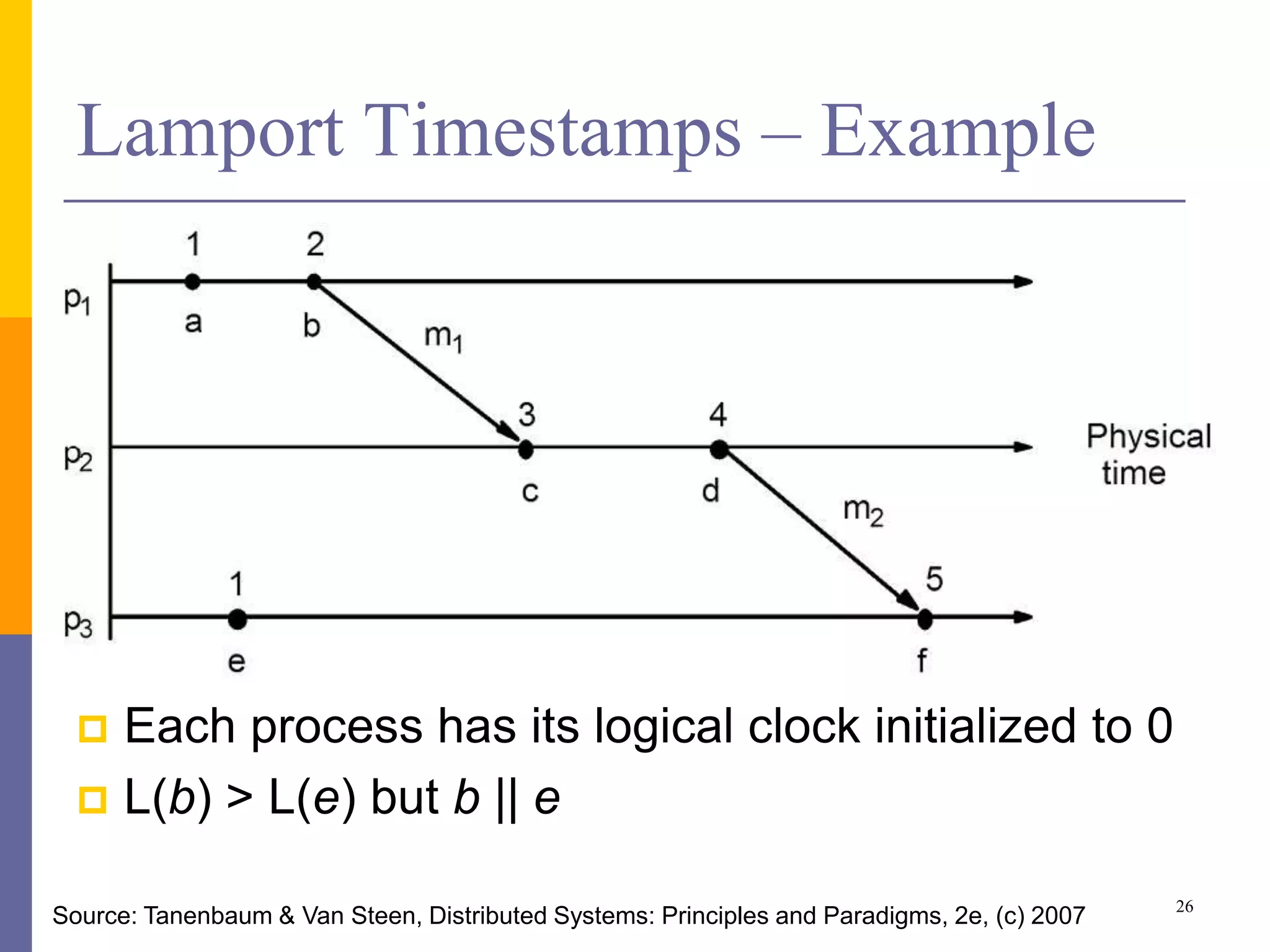
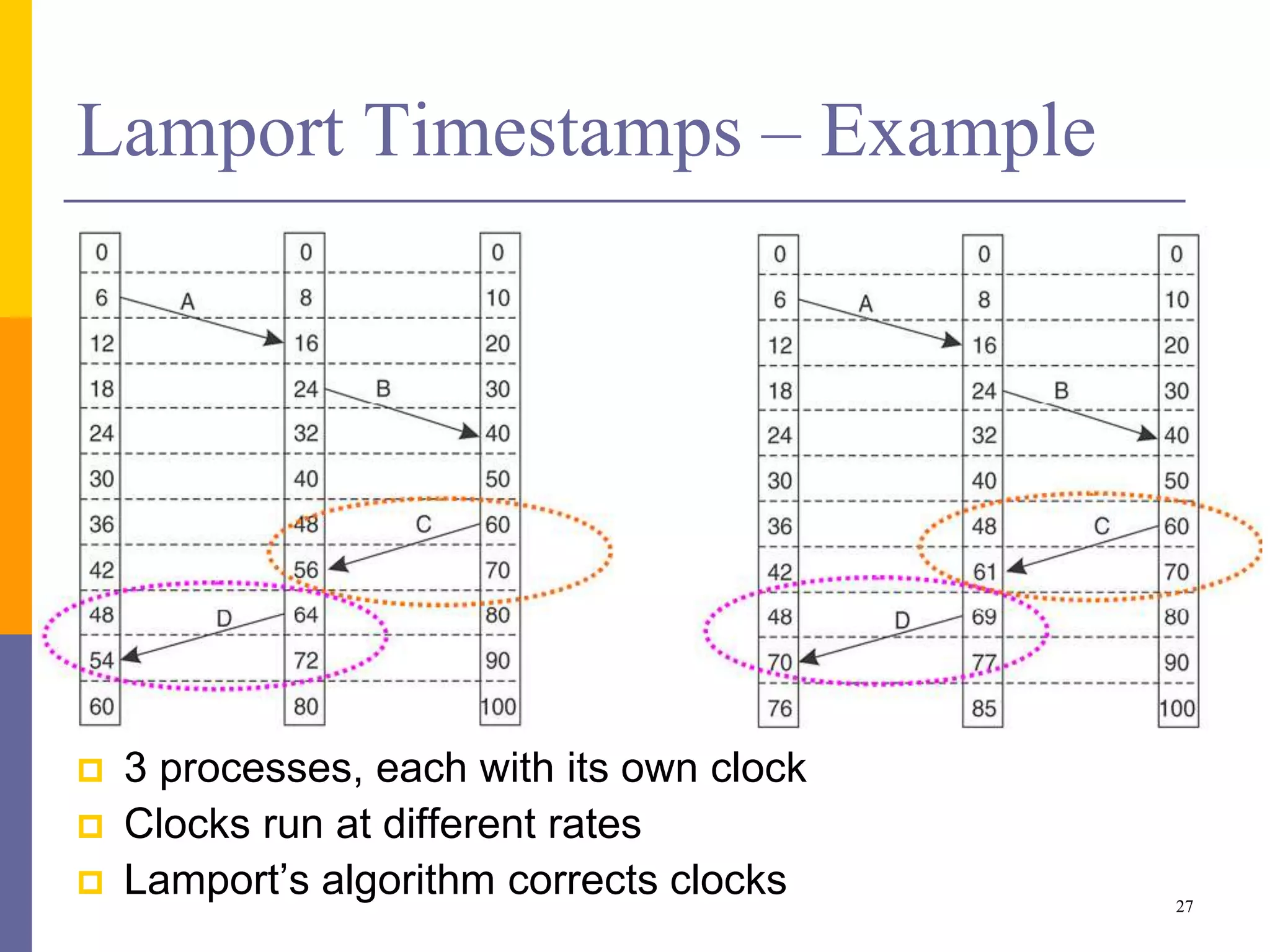
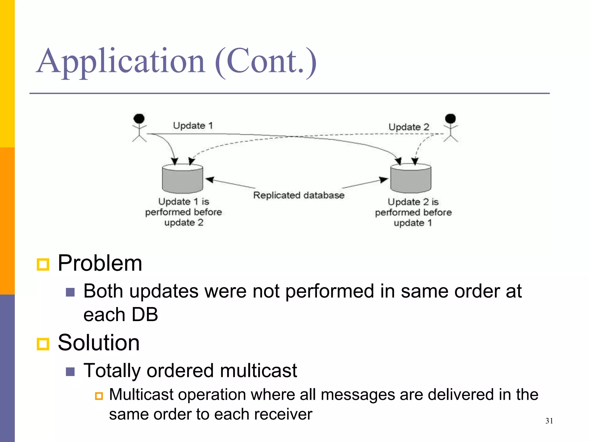
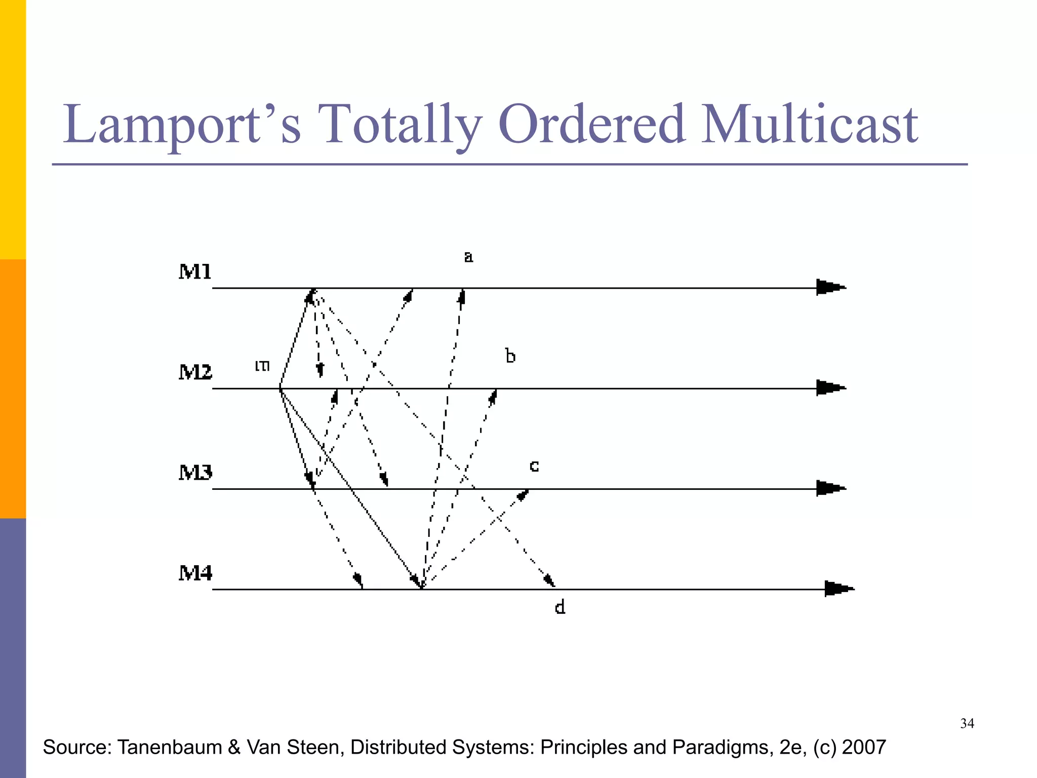
Physical & Logical Clocks
CS4262 Distributed Systems
Dilum Bandara
Dilum.Bandara@uom.lk
Slides adapted from U Uthaiyashankar (WSO2) and Rajkumar Buyya’s (IU)

Outline
 Introduction to synchronization
 Time & clocks
 Synchronizing physical clocks
 Logical time & logical clocks
 Synchronizing logical clocks
 Lamport’s time stamp
 Vector clocks – Not covered
2

Interaction Model
 Computation occurs within processes
 Processes interact by passing messages,
resulting in
 Communication (information flow)
 Coordination (synchronization & ordering of activities)
 2 significant factors affecting interacting
processes in a distributed system
 Communication performance is often a limiting
characteristic
 Impossible to maintain a single global notion of time
3

Interaction Model (Cont.)
 Processes running on different nodes can
associate timestamps with their events
 This timestamp doesn’t make sense globally
 Clock drift
 Differing drift rates
 Complexity & cost of time synchronization
 GPS not accessible inside a building
4

2 Variants of Interaction Model
 Hard to set limits on time taken for
 Process execution
 Message delivery
 Clock drift
 2 simple models
 Synchronous model – based on a strong assumption
of time
 Asynchronous model – makes no assumption about
time
5

Synchronous DS Model
 Defined by following bounds
 Time taken to execute a step of a process has known
lower & upper bounds
 Each message transmitted over a channel is received
within a known bounded time
 Each process has a local clock whose drift rate from
real time has a known bound
6

Asynchronous DS Model
 Defined by assuming no bounds on
 Process execution speeds
 Message transmission delays
 Clock drift rates
 Models Internet very closely
 Any solution that is valid for an asynchronous
DS is also valid for a synchronous DS
 There are many design problems that can’t be solved
for an asynchronous DS, but can be solved when
some aspects of time are used
7

Event Ordering
 Whether an event occurred before, after, or
concurrently with another event at another
process?
 Execution of a system can be described in terms of
events & their ordering
 No need of accurate clocks
 Example
 Consider a mailing list with users X, Y, Z, & A
 User X sends a message with subject “meeting”
 Users Y & Z reply by sending messages with the
subject “Re: meeting”
8

Example – Real-Time Ordering of
Events
9Source: Tanenbaum & Van Steen, Distributed Systems: Principles and Paradigms, 2e, (c) 2007

Example – Inbox of User A
 Due to independent delivery of messages, messages
may be delivered in different order
 If messages m1, m2, m3 carry their time t1, t2, t3, then they
can be displayed accordingly to their time ordering
10

Time in Distributed Systems
 Scenario
 Running UNIX make program which recompiles only source files
whose corresponding object files carry an earlier time stamp
 Differences in time on editing machine & compiler machine & can
result in a file output.o to have a timestamp greater than recently
modified output.c program
 Result
 Modified source program, output.c will not be recompiled
 Programmer???
11

Time & Clocks
 Atomic Time
 Derived from atomic oscillators
 Very accurate
 Astronomical Time
 Based on Earth’s rotation about its axis & around sun
 Period of Earth’s rotation about its axis is gradually
getting longer
 Coordinated Universal Time (UTC)
 Broadcast from land-based radio stations & GPS
12

Clock Drift
 Different rates of counting time
 Physical variations of underlying oscillators
 Variance caused by temperature
 Extremely small differences that accumulate
over a large no of oscillations  Observable
difference in counters
 Drift rate
 Difference in reading between a clock & a nominal
“perfect clock” per unit of time
 10-6 seconds/sec for quartz crystals
 10-7 to 10-8 seconds/sec for high precision quartz
crystals 13

Clock Skew
 When a system has n computers, their n crystals
will oscillate at different rates
 This causes software clocks to gradually get out-
of synch & give different values
 This instantaneous difference in time values is
called clock skew
14

Clock Synchronization
 External synchronization
 If 1 machine has a WWW or GPS receiver, use it to
synchronize others
 Internal synchronization
 If no machines have receivers, each machine keeps
track of its own time
 Then keep all the machines together as well as
possible
 Many clock synchronization algorithms have
been proposed to achieve these goals
 Christian’s Algorithm, Berkeley Algorithm, Averaging
Algorithms, Network Time Protocol, etc. 15

Synchronization in Asynchronous
Systems
 There is no upper bound on message
transmission delays
 e.g., there is no maximum transmission delay for
Internet
 Ttransmit = min + x, where x > 0
 Ttransmit – time taken to transmit m
 Min – minimum time to transmit
 x may not be known in a particular case, but it is
possible to measure a distribution of values for a
particular installation
16

Network Time Protocol (NTP)
 Christian’s & Berkeley algorithms for intranets
 NTP designed for Internet
 Large & variable message delays are handled through
statistical techniques for filtering timing data
 Discriminates between quality of timing data from different
servers
 Redundant servers & redundant paths between servers
 Scalable – handles a large no of clients & servers
 Authentication to ensure trusted time sources
 Synchronization accuracy
 ~10s of milliseconds over Internet paths
 ~1 millisecond on LANs
17

NTP (Cont.)
 Hierarchical network of servers
 Primary servers connected directly to a UTC time source
 Secondary servers synchronized with primary servers
 Servers connected in a logical hierarchy called a synchronization
subnet whose levels are called strata
 Lowest level (leaf) servers execute in users’ workstation
18

Logical Time & Logical Clocks
 Single process
 Events are ordered uniquely by local clock time
 Lamport (1978) pointed out that,
 “since we can’t synchronize clocks perfectly across a
distributed system, we can’t use physical time to find
out order of any arbitrary pair of events within a
distributed system”
 In general, we can use a scheme that is similar
to physical causality, to order some events that
occur in different processes
19

Physical Causality Based Ordering
 If events occur on same process P, then they
occur in the order in which P observes them
 If a & b are events within a single process Pi, and a
occurs before b, then a i b is true
 Whenever a message is sent between
processes, event of sending occurs before event
of receiving
 a = event of a message m being sent by process Pi
 b = event of message m being received
 then, a i b is true
20

Lamport’s Notion of Event Ordering
 Lamport generalized 2 (intuitive) physical-
causality-based event ordering points to obtain
happened-before partial ordering
 A.k.a relation of causal ordering or potential causal
ordering
 Define “happened-before relation” (denoted by
) as follows
 e i e/ for process Pi ⇒ e  e/
 For any message m, send(m)  receive(m)
 e  e/ and e/  e// ⇒ e  e//
21

Happened-Before Relation
22
Source: Tanenbaum & Van Steen, Distributed Systems: Principles and Paradigms, 2e, (c) 2007

Happened-Before Relation
23
 Events a & e that are not ordered by  are concurrent
 Denoted by a || e

Logical Clocks
 Invented by Leslie Lamport to capture
happened-before ordering numerically
 Lamport Logical Clock
 Monotonically increasing software counter
 Value need not have a relationship to any physical
clock
 Each process Pi keeps its own logical clock Li,
which it uses to apply Lamport timestamps to
events
 Li(e) = timestamp of event e at Pi
 L(e) = timestamp of event e at process it occurred
24

Lamport Timestamps
 Processes update their logical clocks & transmit
their logical clock values in messages as follows
 LC1
 Li = Li + 1, before each event is recorded at Pi
 LC2
 When Pi sends a message m, logical clock value t = Li, is piggy-
backed with message
 On receiving (m, t), a process Pj computes
 Lj = max (Lj, t)
 Then computes Lj = Lj + 1 before logically timestamping event
receive(m)
 Thus, e  e/ ⇒ L(e) < L(e/)
 However, L(e) < L(e/) ⇏ e  e/
25

Lamport Timestamps – Example
 Each process has its logical clock initialized to 0
 L(b) > L(e) but b || e
26

Lamport Timestamps – Example
 3 processes, each with its own clock
 Clocks run at different rates
 Lamport’s algorithm corrects clocks 27

Totally Ordered Logical Clocks
 Some pairs of distinct events generated by different
processes have identical Lamport timestamps
 A total order, where all pairs of distinct events are ordered,
can be created by noting IDs of processes
 Suppose,
 (Ti, i) = global logical timestamp for event e at process Pi with local
logical timestamp Ti
 Similarly (Tj, j)
 Then (Ti, i) < (Tj, j) ⇔ Ti < Tj or (Ti = Tj and i < j )
 No general physical significance since process IDs are
arbitrary
 e.g., 2 events in P1 & P2, both with timestamp 40 can be
globally timestamped as 40.1 & 40.2 28

Application of Lamport’s Timestamps
 Consider a database that has been replicated
across several sites
 e.g., a bank account database may be replicated in
Colombo & Kandy
 A query is always forwarded to the nearest copy
(for fast response)
 Update costs are higher since each update must
be carried out at each replica in same order
 Why?
29

Application (Cont.)
 Mr. Perera (lives in Kandy) has Rs. 1,000 in his account
 Mr. Perera wants to deposit Rs. 100 to his account
 At the same time, banking application (in Colombo)
initiates an update to increase account balance with 1%
interest
 Both updates must be carried out at both copies of the
database
 Due to communication delays, we may have following
situation:
 In Kandy DB, Mr. Perera’s deposit is performed before interest
update  (Rs. 1000 + Rs. 100) * 1.01 = Rs. 1,111
 In Colombo DB, interest update is performed before Mr. Perera’s
deposit  (Rs. 1000 * 1.01) + Rs. 100 = Rs. 1,110
30

Application (Cont.)
 Problem
 Both updates were not performed in same order at
each DB
 Solution
 Totally ordered multicast
 Multicast operation where all messages are delivered in the
same order to each receiver 31

Totally Ordered Multicast
 If process Pi sends messages x, y to processes
Pj, Pk ,.. then all processes Pj, Pk … receive
messages in the same order (x, y or y, x)
 This doesn’t imply causal or even FIFO ordering
 Solutions
 Multicast through a central coordinator
 Lamport’s solution
32

Lamport’s Totally Ordered Multicast
 Each multicast has a Lamport time stamp
 All processors store received multicast in a queue
 Order based on time stamp
 Everyone has the same queue
 Assume all messages sent by a sender are received in the
order they were sent & no messages are lost
 A time stamped ACK is sent back
 Timestamp of multicast message < timestamp of ACK
 A process can deliver (act on) the message at the
head of queue only when it has received an ACK
from all other processes
33

Lamport’s Totally Ordered Multicast
34

Summary
 Synchronization is important
 Clock drift & clock skew
 Physical clock synchronization
 Logical time & logical clocks
 Lamport Timestamps
 Vector Clocks
 Totally Ordered Multicast
35

Physical and Logical Clocks

More Related Content

What's hot

Similar to Physical and Logical Clocks

More from Dilum Bandara

Recently uploaded

Physical and Logical Clocks

Editor's Notes