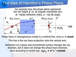
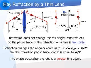
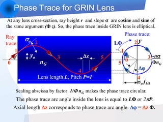
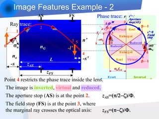
1) Hamilton's phase plane provides a clear way to understand how GRIN lenses shape beams and form images by representing the path of rays and phase traces. 2) Key properties like imaging type, magnification, and beam waist position can be directly derived from analyzing the phase traces within and after the lens. 3) This approach provides simpler, more intuitive formulas than traditional matrix methods and gives insights into aberration correction for beam shaping systems.

1. Gradient Index (GRIN)
Lens Description
on Hamilton’s Phase Plane
Andrei
Tsiboulia
This presentation received The James F. Boulter
BEST PAPER AWARD of the 2003 International
Conference on Applications of Photonic Technology
(ICAPT’ 2003) Photonocs North 2003
Slide show goes automatically

2. Introduction
Hamilton’s phase space is a convenient and natural
media for describing light beam as a whole and to
follow the beam profile transformation by lenses.
Lens design for laser and fiber optics requires
shaping the beam profile, not imaging.
Hamilton’s phase space (phase plane in 2D) is
especially productive for description of GRIN lenses
and aberration correction of beam shaping systems.

3. The Idea of Hamilton’s Phase Plane
y
-n
Phase trace:
This line is the ray trace projection onto the vertical axis.
y’
yoz
Refraction on a plane axis-symmetrical surface changes the ray
direction, but it does not change the phase trace direction,
since according to Snell’s law: noo = n’ ’ =const.
Phase trace in homogeneous media is a vertical line, since  = const.
y Ray trace:
z
no
’
-noo
o n’
n - media refractive index,  - ray tilt angle.
For paraxial rays, the phase plane represents
the ray height y vs. its angular coordinate n .

4. Ray Refraction by a Thin Lens
-n’ ’
h/f’
Refraction changes the angular coordinate: n’’= noo+ h/f’ .
So, the refraction phase trace length is equal to h/f’.
y
n’no
-f f’ (EFL)
Ray trace:
Phase trace:
The phase trace after the lens is a vertical line again.
2 2
-’
3 3
s’
-noo
o
h= -so
1
0 0
1
-s
-n
Refraction does not change the ray height h on the lens.
So the phase trace of the refraction on a lens is horizontal.

5. GRIN Lens Parameters
Ray trace inside GRIN lens is sinusoidal:
y(z) = yo cos( z) + (o / ) sin( z) ; (z) = o cos( z) - yo sin( z).
Front ¼-pitch lens EFL f1/4= -no /ng; rear ¼-pitch EFL f’ 1/4= n’ /ng.
Lens length L, Pitch P=1
yo
o
z -y(z)
Lens axial
index: nG
GRIN lens refractive index (RI) profile is quadratic: n(r)/nG  1 - 0.5 2 r2.
r - the distance from the optical axis, nG - axial RI,  - gradient constant.
y - ray height
- ray tilt angle
z - axial
coordinate
Lens pitch P =L/2
Lens optical power is maximal when pitch P= 1/4.
n’no no & n’ – media RI

6. Lens length L, Pitch P=1
yo
o y
-n
nG0
0
1 1
2 2
33
4
4
5
5
L
z

Axial length z corresponds to phase trace arc angle  = z .
The phase trace arc angle inside the lens is equal to L or 2P.
Scaling abscissa by factor 1/ nG makes the phase trace circular.
Ray
trace:
nG
At any lens cross-section, ray height r and slope  are cosine and sine of
the same argument ( z). So, the phase trace inside GRIN lens is elliptical.
Phase Trace for GRIN Lens
o f1/4
Phase trace:

7. L
l

0 0
1 1
2
3
4
no
nG
y
o
-s’ ’
’
tan= s / f1/4
-n
nG-o f1/4
L
Ray
trace:
2
’ = L gives s’ .
3
4
-l’
-so
 and ’ are defined by
object s and image s’
distances.
Imaging by GRIN Lens
Formulas describing image position and size are simple and clear.
Follow the marginal ray
and related phase trace.
Phase trace:
tan’ = s’ / f’ 1/4
Linear magnification l’  l is the inverse of the angular magnification ’ 
-’ f ’ 1/4
l’ noo -cos
= =l n’’ cos’
Object
distance
-s Image distance s’
’
n’

8. Erect Inverted
Virtual
Virtual
Real
Real
Enlarged
Enlarged
Reduced
Reduced
y
-n
nG
o f1/4
-so

L
s’=∞
Aperture
stop(AS)
s’=∞
AS
s’=0
Field
stop
s’=0
Field
stop




Image Features Vs. Lens Length
The free space phase trace
for marginal ray is vertical.
Free space -parameter is
defined by: tan()=s/f1/4 .
3
2
1
0
5
4
The phase trace inside
GRIN lens is circular.
Points 2 & 4 relate to s’=∞
Image is in infinity
These points divide zones of
erect and inverted image.
Points 3 & 5 relate to s’=0
Image is on the rear lens face
These points divide zones
of real and virtual image.
Points of unit magnification
± divide enlarged and
reduced image zones.

9. Image Features Example - 1
The aperture stop (AS) is at the point 2, where the
marginal ray height is maximal: zAS=()/
The phase trace inside the lens is restricted by the point 3.
The image is inverted, real and enlarged.
zAS
o
Ray trace:
L
n
no
n’
Ray trace:
L
n
no
n’
l
-l’
-s s’
-n’’
no
L
-n’’
no
L
Phase trace:
y
o
-s
-no
no
-n
no
Phase trace:
y
o
-s
-no
no
-n
no
-s’’
’
-s’’
’
0 00 0
1 11 1
2
2
2
2
3 33 3
4-so G
AS Phase trace:
See an example from the next to previous slide.
3
4

10. 4
5
l
-l’
AS FS
Ray trace:
L
n’
no
nG
Phase trace:
o
-s’
-s
0
1
3
2
4
5
Point 4 restricts the phase trace inside the lens.
The image is inverted, virtual and reduced.
The aperture stop (AS) is at the point 2. zAS=()/
The field stop (FS) is at the point 3, where
the marginal ray crosses the optical axis: zFS=()/
zAS
zFS
Image Features Example - 2

11. L
Comparison With Traditional Approach
Usually GRIN lens is substituted
by a regular one:
F’F
H H’
- f f ’
sH -s’H-sF s’F
Optical power L & EFL f and f’ :
L= nGsin(L). (L= -no/f = n’/f’)
Working focal distance SF :
-no/ SF = n’/ SF’= nG tan(L)
Principal planes position SH :
SH /no= -SH‘/n’= tan(L/2)/ nG.
Then the Newton formula zz’=ff’ gives the image position.
Another option –
matrix approach: 
y
LCOSnnLSINnn
LSINnnLCOSy
)()'/()()'/(
)()/()(
'
'
0
0



This chain of formulas gives the same results, as the phase plane
approach, but it is more complicated, and it lacks clarity of the latter.
n’no nG
Rear focal planeFront focal plane
Rear principal planeFront principal plane

12. Ro
o
r


 



-
-
-n
y
Ro
NAo
Gaussian Beam on Phase Plane
Bundle waist is presented on phase plane by ellipse with semi-axes Ro & NAo.
Ro, o and NAo are the waist radius, divergence and NA, no is the index.
At the beam waist, ray height r and slope  are cosine and sine of the
same argument  ( changes between 0 and 2 for different rays):
Ray bundle models Gaussian beam.
 = o sin 
NAo= o no.o  noRo;
Ray trace: r = Ro cos  Phase diagram:

13. Gaussian Beam in Free Space
y
-n
The ellipse area is constant according to Liouville’s theorem. It is equal to .
2Ro
-Ro-o
-NAo
Gaussian beam expands in free space : R2(z)= Ro
2 +( z)2.
Phase points shift vertically according to: y’= yo + z , proportionally to .
Phase
diagram:
Ray trace:
The segment of a vertical line drawn through the ellipse center
and cut by the ellipse gives the beam waist diameter 2Ro.
z cross-section of the beam is presented by the stretched, tilted ellipse.
y Ro R(z)
z

14. Gaussian Beam Inside GRIN Lens
L (P=1/4)
y Phase
diagram:
-n
nG
z

Ellipse rotation angle = z . z – related lens length.
Beam
trace:
Beam waist is on the lens front surface.
The phase diagram is aligned
with coordinate axes.
While the beam propagates in the lens, its phase diagram rotates.
Beam diameter is equal to the vertical projection of the phase diagram.
Divergence is defined by the horizontal one.
This model is really clear and it is consistent with the wave theory.
z
-Ro
-o
o f1/4
R’= o f1/4
n’no
’f’1/4 =Ro

15. Beam Matched With the GRIN Lens
If original beam waist is on the lens front end-face, and Ro= - o f1/4 ,
phase ellipse becomes a circle, rotation does not change its projection.
L (any Pitch)
y
o f1/4 = - Ro
Ro
R’=Ro -n
nG
Ro
The beam waist is on the lens rear end-face for any lens length L.
The GRIN lens is unable to change such a beam. R(z)=const=Ro .
The lens just transfers the beam from its front end-face to the rear one.
Phase diagram:Beam trace:
n’no
R(z)

16. Aberration Correction – (Laser) Beams
There are few features making difference between aberration correction
for beam shaping and imaging systems. Some of them are:
1. Focused and original beams must have similar energy distribution.
It does not necessarily require image.
Recombined rays may still give the required distribution.
2. We do not care about ray tilt in imaging system.
For beam shaping, angular and liner characteristics are equally important.
That is why phase space helps in beam shaping optical system design.
3. There is no aperture stop in beam shaping system. On the other hand,
position of the aperture stop in imaging system affects its aberrations.
These features imply different strategy for aberration correction of
beam shaping optical systems.

17. Conclusion
•These formulas give clearer understanding and
facilitate solving of practical problems.
•Hamilton’s phase plane gives vivid and clear illustration
of GRIN lens imaging and beam shaping properties.
•Hamilton’s phase plane allows a simple derivation
of clear direct formulas for parameters of GRIN lens
created image and transformed Gaussian beam.
•Hamilton’s phase plane gives a productive approach to
aberration correction of beam shaping optical systems.