Perry’s Chemical Engineers’ Handbook 7ma Ed Chap 06

FLUID DYNAMICS
Nature of Fluids . . . . . . . . . . . . . . . . . . . . . . . . . . . . . . . . . . . . . . . . . . . . 6-4
Deformation and Stress . . . . . . . . . . . . . . . . . . . . . . . . . . . . . . . . . . . . 6-4
Viscosity. . . . . . . . . . . . . . . . . . . . . . . . . . . . . . . . . . . . . . . . . . . . . . . . . 6-4
Rheology . . . . . . . . . . . . . . . . . . . . . . . . . . . . . . . . . . . . . . . . . . . . . . . . 6-4
Kinematics of Fluid Flow. . . . . . . . . . . . . . . . . . . . . . . . . . . . . . . . . . . . . 6-5
Velocity . . . . . . . . . . . . . . . . . . . . . . . . . . . . . . . . . . . . . . . . . . . . . . . . . 6-5
Compressible and Incompressible Flow . . . . . . . . . . . . . . . . . . . . . . . 6-5
Streamlines, Pathlines, and Streaklines . . . . . . . . . . . . . . . . . . . . . . . . 6-5
One-dimensional Flow . . . . . . . . . . . . . . . . . . . . . . . . . . . . . . . . . . . . . 6-5
Rate of Deformation Tensor . . . . . . . . . . . . . . . . . . . . . . . . . . . . . . . . 6-5
Vorticity . . . . . . . . . . . . . . . . . . . . . . . . . . . . . . . . . . . . . . . . . . . . . . . . . 6-5
Laminar and Turbulent Flow, Reynolds Number. . . . . . . . . . . . . . . . 6-6
Conservation Equations . . . . . . . . . . . . . . . . . . . . . . . . . . . . . . . . . . . . . . 6-6
Macroscopic and Microscopic Balances . . . . . . . . . . . . . . . . . . . . . . . 6-6
Macroscopic Equations . . . . . . . . . . . . . . . . . . . . . . . . . . . . . . . . . . . . 6-6
Mass Balance. . . . . . . . . . . . . . . . . . . . . . . . . . . . . . . . . . . . . . . . . . . . . 6-6
Momentum Balance . . . . . . . . . . . . . . . . . . . . . . . . . . . . . . . . . . . . . . . 6-6
Total Energy Balance . . . . . . . . . . . . . . . . . . . . . . . . . . . . . . . . . . . . . . 6-7
Mechanical Energy Balance, Bernoulli Equation. . . . . . . . . . . . . . . . 6-7
Microscopic Balance Equations. . . . . . . . . . . . . . . . . . . . . . . . . . . . . . 6-7
Mass Balance, Continuity Equation. . . . . . . . . . . . . . . . . . . . . . . . . . . 6-7
Stress Tensor. . . . . . . . . . . . . . . . . . . . . . . . . . . . . . . . . . . . . . . . . . . . . 6-7
Cauchy Momentum and Navier-Stokes Equations . . . . . . . . . . . . . . . 6-8
Examples. . . . . . . . . . . . . . . . . . . . . . . . . . . . . . . . . . . . . . . . . . . . . . . . 6-8
Example 1: Force Exerted on a Reducing Bend. . . . . . . . . . . . . . . . . 6-8
Example 2: Simplified Ejector . . . . . . . . . . . . . . . . . . . . . . . . . . . . . . . 6-8
Example 3: Venturi Flowmeter . . . . . . . . . . . . . . . . . . . . . . . . . . . . . . 6-9
Example 4: Plane Poiseuille Flow . . . . . . . . . . . . . . . . . . . . . . . . . . . . 6-9
Incompressible Flow in Pipes and Channels. . . . . . . . . . . . . . . . . . . . . . 6-9
Mechanical Energy Balance. . . . . . . . . . . . . . . . . . . . . . . . . . . . . . . . . 6-9
Friction Factor and Reynolds Number . . . . . . . . . . . . . . . . . . . . . . . . 6-9
Laminar and Turbulent Flow. . . . . . . . . . . . . . . . . . . . . . . . . . . . . . . . 6-10
Velocity Profiles . . . . . . . . . . . . . . . . . . . . . . . . . . . . . . . . . . . . . . . . . . 6-11
Entrance and Exit Effects . . . . . . . . . . . . . . . . . . . . . . . . . . . . . . . . . . 6-11
Residence Time Distribution. . . . . . . . . . . . . . . . . . . . . . . . . . . . . . . . 6-11
Noncircular Channels. . . . . . . . . . . . . . . . . . . . . . . . . . . . . . . . . . . . . . 6-12
Nonisothermal Flow. . . . . . . . . . . . . . . . . . . . . . . . . . . . . . . . . . . . . . . 6-12
Open Channel Flow . . . . . . . . . . . . . . . . . . . . . . . . . . . . . . . . . . . . . . . 6-12
Non-Newtonian Flow. . . . . . . . . . . . . . . . . . . . . . . . . . . . . . . . . . . . . . 6-13
Economic Pipe Diameter, Turbulent Flow . . . . . . . . . . . . . . . . . . . . . 6-14
Economic Pipe Diameter, Laminar Flow . . . . . . . . . . . . . . . . . . . . . . 6-14
Vacuum Flow . . . . . . . . . . . . . . . . . . . . . . . . . . . . . . . . . . . . . . . . . . . . 6-14
Molecular Flow. . . . . . . . . . . . . . . . . . . . . . . . . . . . . . . . . . . . . . . . . . . 6-15
Slip Flow . . . . . . . . . . . . . . . . . . . . . . . . . . . . . . . . . . . . . . . . . . . . . . . . 6-15
Frictional Losses in Pipeline Elements . . . . . . . . . . . . . . . . . . . . . . . . . . 6-16
Equivalent Length and Velocity Head Methods. . . . . . . . . . . . . . . . . 6-16
Contraction and Entrance Losses . . . . . . . . . . . . . . . . . . . . . . . . . . . . 6-16
Example 5: Entrance Loss . . . . . . . . . . . . . . . . . . . . . . . . . . . . . . . . . . 6-16
Expansion and Exit Losses . . . . . . . . . . . . . . . . . . . . . . . . . . . . . . . . . . 6-17
Fittings and Valves . . . . . . . . . . . . . . . . . . . . . . . . . . . . . . . . . . . . . . . . 6-17
Example 6: Losses with Fittings and Valves . . . . . . . . . . . . . . . . . . . . 6-17
Curved Pipes and Coils . . . . . . . . . . . . . . . . . . . . . . . . . . . . . . . . . . . . 6-18
Screens . . . . . . . . . . . . . . . . . . . . . . . . . . . . . . . . . . . . . . . . . . . . . . . . . 6-19
Jet Behavior. . . . . . . . . . . . . . . . . . . . . . . . . . . . . . . . . . . . . . . . . . . . . . . . 6-20
Flow through Orifices. . . . . . . . . . . . . . . . . . . . . . . . . . . . . . . . . . . . . . . . 6-21
Compressible Flow. . . . . . . . . . . . . . . . . . . . . . . . . . . . . . . . . . . . . . . . . . 6-22
Mach Number and Speed of Sound . . . . . . . . . . . . . . . . . . . . . . . . . . 6-22
Isothermal Gas Flow in Pipes and Channels. . . . . . . . . . . . . . . . . . . . 6-22
Adiabatic Frictionless Nozzle Flow . . . . . . . . . . . . . . . . . . . . . . . . . . . 6-22
Example 7: Flow through Frictionless Nozzle . . . . . . . . . . . . . . . . . . 6-23
Adiabatic Flow with Friction in a Duct of Constant
Cross Section. . . . . . . . . . . . . . . . . . . . . . . . . . . . . . . . . . . . . . . . . . . 6-23
Example 8: Compressible Flow with Friction Losses. . . . . . . . . . . . . 6-25
Convergent/Divergent Nozzles (De Laval Nozzles) . . . . . . . . . . . . . . 6-25
Multiphase Flow. . . . . . . . . . . . . . . . . . . . . . . . . . . . . . . . . . . . . . . . . . . . 6-26
Liquids and Gases. . . . . . . . . . . . . . . . . . . . . . . . . . . . . . . . . . . . . . . . . 6-26
Gases and Solids . . . . . . . . . . . . . . . . . . . . . . . . . . . . . . . . . . . . . . . . . . 6-29
Fluid Distribution. . . . . . . . . . . . . . . . . . . . . . . . . . . . . . . . . . . . . . . . . . . 6-32
Perforated-Pipe Distributors . . . . . . . . . . . . . . . . . . . . . . . . . . . . . . . . 6-32
Example 9: Pipe Distributor . . . . . . . . . . . . . . . . . . . . . . . . . . . . . . . . 6-33
Slot Distributors . . . . . . . . . . . . . . . . . . . . . . . . . . . . . . . . . . . . . . . . . . 6-33
Turning Vanes . . . . . . . . . . . . . . . . . . . . . . . . . . . . . . . . . . . . . . . . . . . . 6-33
Perforated Plates and Screens . . . . . . . . . . . . . . . . . . . . . . . . . . . . . . . 6-33
Beds of Solids . . . . . . . . . . . . . . . . . . . . . . . . . . . . . . . . . . . . . . . . . . . . 6-34
Other Flow Straightening Devices . . . . . . . . . . . . . . . . . . . . . . . . . . . 6-34
Fluid Mixing . . . . . . . . . . . . . . . . . . . . . . . . . . . . . . . . . . . . . . . . . . . . . . . 6-34
Stirred Tank Agitation. . . . . . . . . . . . . . . . . . . . . . . . . . . . . . . . . . . . . . 6-34
Pipeline Mixing. . . . . . . . . . . . . . . . . . . . . . . . . . . . . . . . . . . . . . . . . . . 6-35
Tube Banks . . . . . . . . . . . . . . . . . . . . . . . . . . . . . . . . . . . . . . . . . . . . . . . . 6-36
Turbulent Flow . . . . . . . . . . . . . . . . . . . . . . . . . . . . . . . . . . . . . . . . . . . 6-36
Transition Region . . . . . . . . . . . . . . . . . . . . . . . . . . . . . . . . . . . . . . . . . 6-38
6-1
Section 6
Fluid and Particle Dynamics*
James N. Tilton, Ph.D., P.E., Senior Consultant, Process Engineering, E. I. du Pont de
Nemours & Co.; Member, American Institute of Chemical Engineers; Registered Professional
Engineer (Delaware)
* The author acknowledges the contribution of B. C. Sakiadis, editor of this section in the sixth edition of the Handbook.
Copyright © 1999 by The McGraw-Hill Companies, Inc. All rights reserved. Use of
this product is subject to the terms of its license agreement. Click here to view.

Laminar Region . . . . . . . . . . . . . . . . . . . . . . . . . . . . . . . . . . . . . . . . . . 6-38
Beds of Solids . . . . . . . . . . . . . . . . . . . . . . . . . . . . . . . . . . . . . . . . . . . . . . 6-38
Fixed Beds of Granular Solids . . . . . . . . . . . . . . . . . . . . . . . . . . . . . . . 6-38
Porous Media . . . . . . . . . . . . . . . . . . . . . . . . . . . . . . . . . . . . . . . . . . . . 6-39
Tower Packings . . . . . . . . . . . . . . . . . . . . . . . . . . . . . . . . . . . . . . . . . . . 6-40
Fluidized Beds . . . . . . . . . . . . . . . . . . . . . . . . . . . . . . . . . . . . . . . . . . . 6-40
Boundary Layer Flows . . . . . . . . . . . . . . . . . . . . . . . . . . . . . . . . . . . . . . . 6-40
Flat Plate, Zero Angle of Incidence. . . . . . . . . . . . . . . . . . . . . . . . . . . 6-40
Cylindrical Boundary Layer . . . . . . . . . . . . . . . . . . . . . . . . . . . . . . . . . 6-40
Continuous Flat Surface. . . . . . . . . . . . . . . . . . . . . . . . . . . . . . . . . . . . 6-40
Continuous Cylindrical Surface . . . . . . . . . . . . . . . . . . . . . . . . . . . . . . 6-41
Vortex Shedding . . . . . . . . . . . . . . . . . . . . . . . . . . . . . . . . . . . . . . . . . . . . 6-41
Coating Flows . . . . . . . . . . . . . . . . . . . . . . . . . . . . . . . . . . . . . . . . . . . . . . 6-42
Falling Films . . . . . . . . . . . . . . . . . . . . . . . . . . . . . . . . . . . . . . . . . . . . . . . 6-42
Minimum Wetting Rate . . . . . . . . . . . . . . . . . . . . . . . . . . . . . . . . . . . . 6-42
Laminar Flow . . . . . . . . . . . . . . . . . . . . . . . . . . . . . . . . . . . . . . . . . . . . 6-42
Turbulent Flow . . . . . . . . . . . . . . . . . . . . . . . . . . . . . . . . . . . . . . . . . . . 6-43
Effect of Surface Traction . . . . . . . . . . . . . . . . . . . . . . . . . . . . . . . . . . 6-43
Flooding . . . . . . . . . . . . . . . . . . . . . . . . . . . . . . . . . . . . . . . . . . . . . . . . 6-43
Hydraulic Transients. . . . . . . . . . . . . . . . . . . . . . . . . . . . . . . . . . . . . . . . . 6-44
Water Hammer . . . . . . . . . . . . . . . . . . . . . . . . . . . . . . . . . . . . . . . . . . . 6-44
Example 10: Response to Instantaneous Valve Closing . . . . . . . . . . . 6-44
Pulsating Flow. . . . . . . . . . . . . . . . . . . . . . . . . . . . . . . . . . . . . . . . . . . . 6-44
Cavitation . . . . . . . . . . . . . . . . . . . . . . . . . . . . . . . . . . . . . . . . . . . . . . . 6-44
Turbulence . . . . . . . . . . . . . . . . . . . . . . . . . . . . . . . . . . . . . . . . . . . . . . . . 6-45
Time Averaging. . . . . . . . . . . . . . . . . . . . . . . . . . . . . . . . . . . . . . . . . . . 6-45
Closure Models. . . . . . . . . . . . . . . . . . . . . . . . . . . . . . . . . . . . . . . . . . . 6-46
Eddy Spectrum. . . . . . . . . . . . . . . . . . . . . . . . . . . . . . . . . . . . . . . . . . . 6-46
Computational Fluid Dynamics. . . . . . . . . . . . . . . . . . . . . . . . . . . . . . . . 6-47
Dimensionless Groups . . . . . . . . . . . . . . . . . . . . . . . . . . . . . . . . . . . . . . . 6-48
PARTICLE DYNAMICS
Drag Coefficient . . . . . . . . . . . . . . . . . . . . . . . . . . . . . . . . . . . . . . . . . . . . 6-50
Terminal Settling Velocity . . . . . . . . . . . . . . . . . . . . . . . . . . . . . . . . . . . . 6-50
Spherical Particles . . . . . . . . . . . . . . . . . . . . . . . . . . . . . . . . . . . . . . . . 6-50
Nonspherical Rigid Particles . . . . . . . . . . . . . . . . . . . . . . . . . . . . . . . . 6-51
Hindered Settling . . . . . . . . . . . . . . . . . . . . . . . . . . . . . . . . . . . . . . . . . 6-52
Time-dependent Motion . . . . . . . . . . . . . . . . . . . . . . . . . . . . . . . . . . . 6-52
Gas Bubbles . . . . . . . . . . . . . . . . . . . . . . . . . . . . . . . . . . . . . . . . . . . . . 6-53
Liquid Drops in Liquids. . . . . . . . . . . . . . . . . . . . . . . . . . . . . . . . . . . . 6-53
Liquid Drops in Gases . . . . . . . . . . . . . . . . . . . . . . . . . . . . . . . . . . . . . 6-54
Wall Effects. . . . . . . . . . . . . . . . . . . . . . . . . . . . . . . . . . . . . . . . . . . . . . 6-54
6-2 FLUID AND PARTICLE DYNAMICS

6-3
Nomenclature and Units*
In this listing, symbols used in this section are defined in a general way and appropriate SI units are given. Specific definitions, as denoted by subscripts, are stated at
the place of application in the section. Some specialized symbols used in the section are defined only at the place of application. Some symbols have more than one
definition; the appropriate one is identified at the place of application.
U.S. customary
Symbol Definition SI units units
a Pressure wave velocity m/s ft/s
A Area m2
ft2
b Wall thickness m in
b Channel width m ft
c Acoustic velocity m/s ft/s
cf Friction coefficient Dimensionless Dimensionless
C Conductance m3
/s ft3
/s
Ca Capillary number Dimensionless Dimensionless
C0 Discharge coefficient Dimensionless Dimensionless
CD Drag coefficient Dimensionless Dimensionless
d Diameter m ft
D Diameter m ft
De Dean number Dimensionless Dimensionless
Dij Deformation rate tensor 1/s 1/s
components
E Elastic modulus Pa lbf/in2
Ėv Energy dissipation rate J/s ft ⋅ lbf/s
Eo Eotvos number Dimensionless Dimensionless
f Fanning friction factor Dimensionless Dimensionless
f Vortex shedding frequency 1/s 1/s
F Force N lbf
F Cumulative residence time Dimensionless Dimensionless
distribution
Fr Froude number Dimensionless Dimensionless
g Acceleration of gravity m/s2
ft/s2
G Mass flux kg/(m2
⋅ s) lbm/(ft2
⋅ s)
h Enthalpy per unit mass J/kg Btu/lbm
h Liquid depth m ft
k Ratio of specific heats Dimensionless Dimensionless
k Kinetic energy of turbulence J/kg ft ⋅ lbf/lbm
K Power law coefficient kg/(m ⋅ s2 − n
) lbm/(ft ⋅ s2 − n
)
lv Viscous losses per unit mass J/kg ft ⋅ lbf/lbm
L Length m ft
ṁ Mass flow rate kg/s lbm/s
M Mass kg lbm
M Mach number Dimensionless Dimensionless
M Morton number Dimensionless Dimensionless
Mw Molecular weight kg/kgmole lbm/lbmole
n Power law exponent Dimensionless Dimensionless
Nb Blend time number Dimensionless Dimensionless
ND Best number Dimensionless Dimensionless
NP Power number Dimensionless Dimensionless
NQ Pumping number Dimensionless Dimensionless
p Pressure Pa lbf/in2
q Entrained flow rate m3
/s ft3
/s
Q Volumetric flow rate m3
/s ft3
/s
Q Throughput (vacuum flow) Pa ⋅ m3
/s lbf ⋅ ft3
/s
δQ Heat input per unit mass J/kg Btu/lbm
r Radial coordinate m ft
R Radius m ft
R Ideal gas universal constant J/(kgmole ⋅ K) Btu/(lbmole ⋅ R)
Ri Volume fraction of phase i Dimensionless Dimensionless
Re Reynolds number Dimensionless Dimensionless
s Density ratio Dimensionless Dimensionless
U.S. customary
Symbol Definition SI units units
s Entropy per unit mass J/(kg ⋅ K) Btu/(lbm ⋅ R)
S Slope Dimensionless Dimensionless
S Pumping speed m3
/s ft3
/s
S Surface area per unit volume l/m l/ft
St Strouhal number Dimensionless Dimensionless
t Time s s
t Force per unit area Pa lbf/in2
T Absolute temperature K R
u Internal energy per unit mass J/kg Btu/lbm
u Velocity m/s ft/s
U Velocity m/s ft/s
v Velocity m/s ft/s
V Velocity m/s ft/s
V Volume m3
ft3
We Weber number Dimensionless Dimensionless
Ẇs Rate of shaft work J/s Btu/s
δWs Shaft work per unit mass J/kg Btu/lbm
x Cartesian coordinate m ft
y Cartesian coordinate m ft
z Cartesian coordinate m ft
z Elevation m ft
Greek symbols
α Velocity profile factor Dimensionless Dimensionless
α Included angle Radians Radians
β Velocity profile factor Dimensionless Dimensionless
β Bulk modulus of elasticity Pa lbf/in2
γ̇ Shear rate l/s l/s
Γ Mass flow rate kg/(m ⋅ s) lbm/(ft ⋅ s)
per unit width
δ Boundary layer or film m ft
thickness
δij Kronecker delta Dimensionless Dimensionless
e Pipe roughness m ft
e Void fraction Dimensionless Dimensionless
e Turbulent dissipation rate J/(kg ⋅ s) ft ⋅ lbf/(lbm ⋅ s)
θ Residence time s s
θ Angle Radians Radians
λ Mean free path m ft
µ Viscosity Pa ⋅ s lbm/(ft ⋅ s)
ν Kinematic viscosity m2
/s ft2
/s
ρ Density kg/m3
lbm/ft3
σ Surface tension N/m lbf/ft
σ Cavitation number Dimensionless Dimensionless
σij Components of total Pa lbf/in2
stress tensor
τ Shear stress Pa lbf/in2
τ Time period s s
τij Components of deviatoric Pa lbf/in2
stress tensor
Φ Energy dissipation rate J/(m3
⋅ s) ft ⋅ lbf/(ft3
⋅ s)
per unit volume
φ Angle of inclination Radians Radians
ω Vorticity 1/s 1/s
*Note that with U.S. Customary units, the conversion factor gc may be required to make equations in this section dimensionally consistent; gc = 32.17 (lbm⋅ft)/lbf⋅s2
).

GENERAL REFERENCES: Batchelor, An Introduction to Fluid Dynamics, Cam-
bridge University, Cambridge, 1967; Bird, Stewart, and Lightfoot, Transport
Phenomena, Wiley, New York, 1960; Brodkey, The Phenomena of Fluid Motions,
Addison-Wesley, Reading, Mass., 1967; Denn, Process Fluid Mechanics, Pren-
tice-Hall, Englewood Cliffs, N.J., 1980; Landau and Lifshitz, Fluid Mechanics,
2d ed., Pergamon, 1987; Govier and Aziz, The Flow of Complex Mixtures in
Pipes, Van Nostrand Reinhold, New York, 1972, Krieger, Huntington, N.Y.,
1977; Panton, Incompressible Flow, Wiley, New York, 1984; Schlichting, Bound-
ary Layer Theory, 8th ed., McGraw-Hill, New York, 1987; Shames, Mechanics
of Fluids, 3d ed., McGraw-Hill, New York, 1992; Streeter, Handbook of Fluid
Dynamics, McGraw-Hill, New York, 1971; Streeter and Wylie, Fluid Mechanics,
8th ed., McGraw-Hill, New York, 1985; Vennard and Street, Elementary Fluid
Mechanics, 5th ed., Wiley, New York, 1975; Whitaker, Introduction to Fluid
Mechanics, Prentice-Hall, Englewood Cliffs, N.J., 1968, Krieger, Huntington,
N.Y., 1981.
NATURE OF FLUIDS
Deformation and Stress A fluid is a substance which undergoes
continuous deformation when subjected to a shear stress. Figure 6-1
illustrates this concept. A fluid is bounded by two large parallel plates,
of area A, separated by a small distance H. The bottom plate is held
fixed. Application of a force F to the upper plate causes it to move at a
velocity U. The fluid continues to deform as long as the force is applied,
unlike a solid, which would undergo only a finite deformation.
The force is directly proportional to the area of the plate; the shear
stress is τ = F/A. Within the fluid, a linear velocity profile u = Uy/H is
established; due to the no-slip condition, the fluid bounding the
lower plate has zero velocity and the fluid bounding the upper plate
moves at the plate velocity U. The velocity gradient γ̇ = du/dy is called
the shear rate for this flow. Shear rates are usually reported in units
of reciprocal seconds. The flow in Fig. 6-1 is a simple shear flow.
Viscosity The ratio of shear stress to shear rate is the viscosity, µ.
µ = (6-1)
The SI units of viscosity are kg/(m ⋅ s) or Pa ⋅ s (pascal second). The cgs
unit for viscosity is the poise; 1 Pa ⋅ s equals 10 poise or 1000 cen-
tipoise (cP) or 0.672 lbm/(ft ⋅ s). The terms absolute viscosity and
shear viscosity are synonymous with the viscosity as used in Eq. (6-1).
Kinematic viscosity ν ; µ/ρ is the ratio of viscosity to density. The SI
units of kinematic viscosity are m2
/s. The cgs stoke is 1 cm2
/s.
Rheology In general, fluid flow patterns are more complex than
the one shown in Fig. 6-1, as is the relationship between fluid defor-
mation and stress. Rheology is the discipline of fluid mechanics which
studies this relationship. One goal of rheology is to obtain constitu-
tive equations by which stresses may be computed from deformation
rates. For simplicity, fluids may be classified into rheological types in
reference to the simple shear flow of Fig. 6-1. Complete definitions
require extension to multidimensional flow. For more information,
several good references are available, including Bird, Armstrong, and
Hassager, (Dynamics of Polymeric Liquids, vol. 1: Fluid Mechanics,
Wiley, New York, 1977); Metzner, (“Flow of Non-Newtonian Fluids”
in Streeter, Handbook of Fluid Dynamics, McGraw-Hill, New York,
1971); and Skelland (Non-Newtonian Flow and Heat Transfer, Wiley,
New York, 1967).
τ
}
γ̇
Fluids without any solidlike elastic behavior do not undergo any
reverse deformation when shear stress is removed, and are called
purely viscous fluids. The shear stress depends only on the rate of
deformation, and not on the extent of deformation (strain). Those
which exhibit both viscous and elastic properties are called viscoelas-
tic fluids.
Purely viscous fluids are further classified into time-independent
and time-dependent fluids. For time-independent fluids, the shear
stress depends only on the instantaneous shear rate. The shear stress
for time-dependent fluids depends on the past history of the rate of
deformation, as a result of structure or orientation buildup or break-
down during deformation.
A rheogram is a plot of shear stress versus shear rate for a fluid in
simple shear flow, such as that in Fig. 6-1. Rheograms for several types
of time-independent fluids are shown in Fig. 6-2. The Newtonian
fluid rheogram is a straight line passing through the origin. The slope
of the line is the viscosity. For a Newtonian fluid, the viscosity is inde-
pendent of shear rate, and may depend only on temperature and per-
haps pressure. By far, the Newtonian fluid is the largest class of fluid
of engineering importance. Gases and low molecular weight liquids
are generally Newtonian. Newton’s law of viscosity is a rearrangement
of Eq. (6-1) in which the viscosity is a constant:
τ = µγ̇ = µ (6-2)
All fluids for which the viscosity varies with shear rate are non-
Newtonian fluids. For non-Newtonian fluids the viscosity, defined
as the ratio of shear stress to shear rate, is often called the apparent
viscosity to emphasize the distinction from Newtonian behavior.
Purely viscous, time-independent fluids, for which the apparent vis-
cosity may be expressed as a function of shear rate, are called gener-
alized Newtonian fluids.
Non-Newtonian fluids include those for which a finite stress τy is
required before continuous deformation occurs; these are called
yield-stress materials. The Bingham plastic fluid is the simplest
yield-stress material; its rheogram has a constant slope µ∞, called the
infinite shear viscosity.
τ = τy + µ∞γ̇ (6-3)
Highly concentrated suspensions of fine solid particles frequently
exhibit Bingham plastic behavior.
Shear-thinning fluids are those for which the slope of the
rheogram decreases with increasing shear rate. These fluids have also
been called pseudoplastic, but this terminology is outdated and dis-
couraged. Many polymer melts and solutions, as well as some solids
suspensions, are shear-thinning. Shear-thinning fluids without yield
stresses typically obey a power law model over a range of shear rates.
τ = Kγ̇ n
(6-4)
The apparent viscosity is
µ = Kγ̇ n − 1
(6-5)
du
}
dy
FLUID DYNAMICS
y
x
H
V
F
A
FIG. 6-1 Deformation of a fluid subjected to a shear stress.
Shear rate |du/dy|
Shear
stress
τ
τy
n
a
i
n
o
t
w
e
N
c
i
t
s
a
l
p
m
a
h
g
n
i
B
c
i
t
s
a
l
p
o
d
u
e
s
P
t
n
a
t
a
l
i
D
FIG. 6-2 Shear diagrams.

The factor K is the consistency index or power law coefficient, and
n is the power law exponent. The exponent n is dimensionless, while
K is in units of kg/(m ⋅ s2 − n
). For shear-thinning fluids, n < 1. The
power law model typically provides a good fit to data over a range of
one to two orders of magnitude in shear rate; behavior at very low and
very high shear rates is often Newtonian. Shear-thinning power law
fluids with yield stresses are sometimes called Herschel-Bulkley fluids.
Numerous other rheological model equations for shear-thinning fluids
are in common use.
Dilatant, or shear-thickening, fluids show increasing viscosity with
increasing shear rate. Over a limited range of shear rate, they may be
described by the power law model with n > 1. Dilatancy is rare,
observed only in certain concentration ranges in some particle sus-
pensions (Govier and Aziz, pp. 33–34). Extensive discussions of dila-
tant suspensions, together with a listing of dilatant systems, are given
by Green and Griskey (Trans. Soc. Rheol, 12[1], 13–25 [1968]);
Griskey and Green (AIChE J., 17, 725–728 [1971]); and Bauer and
Collins (“Thixotropy and Dilatancy,” in Eirich, Rheology, vol. 4, Aca-
demic, New York, 1967).
Time-dependent fluids are those for which structural rearrange-
ments occur during deformation at a rate too slow to maintain equi-
librium configurations. As a result, shear stress changes with duration
of shear. Thixotropic fluids, such as mayonnaise, clay suspensions
used as drilling muds, and some paints and inks, show decreasing
shear stress with time at constant shear rate. A detailed description of
thixotropic behavior and a list of thixotropic systems is found in Bauer
and Collins (ibid.).
Rheopectic behavior is the opposite of thixotropy. Shear stress
increases with time at constant shear rate. Rheopectic behavior has
been observed in bentonite sols, vanadium pentoxide sols, and gyp-
sum suspensions in water (Bauer and Collins, ibid.) as well as in some
polyester solutions (Steg and Katz, J. Appl. Polym. Sci., 9, 3, 177
[1965]).
Viscoelastic fluids exhibit elastic recovery from deformation when
stress is removed. Polymeric liquids comprise the largest group of flu-
ids in this class. A property of viscoelastic fluids is the relaxation time,
which is a measure of the time required for elastic effects to decay.
Viscoelastic effects may be important with sudden changes in rates of
deformation, as in flow startup and stop, rapidly oscillating flows, or as
a fluid passes through sudden expansions or contractions where accel-
erations occur. In many fully developed flows where such effects are
absent, viscoelastic fluids behave as if they were purely viscous. In vis-
coelastic flows, normal stresses perpendicular to the direction of shear
are different from those in the parallel direction. These give rise to
such behaviors as the Weissenberg effect, in which fluid climbs up a
shaft rotating in the fluid, and die swell, where a stream of fluid issu-
ing from a tube may expand to two or more times the tube diameter.
A parameter indicating whether viscoelastic effects are important is
the Deborah number, which is the ratio of the characteristic relax-
ation time of the fluid to the characteristic time scale of the flow. For
small Deborah numbers, the relaxation is fast compared to the char-
acteristic time of the flow, and the fluid behavior is purely viscous. For
very large Deborah numbers, the behavior closely resembles that of
an elastic solid.
Analysis of viscoelastic flows is very difficult. Simple constitutive
equations are unable to describe all the material behavior exhibited by
viscoelastic fluids even in geometrically simple flows. More complex
constitutive equations may be more accurate, but become exceedingly
difficult to apply, especially for complex geometries, even with
advanced numerical methods. For good discussions of viscoelastic
fluid behavior, including various types of constitutive equations, see
Bird, Armstrong, and Hassager (Dynamics of Polymeric Liquids, vol.
1: Fluid Mechanics, vol. 2: Kinetic Theory, Wiley, New York, 1977);
Middleman (The Flow of High Polymers, Interscience (Wiley) New
York, 1968); or Astarita and Marrucci (Principles of Non-Newtonian
Fluid Mechanics, McGraw-Hill, New York, 1974).
Polymer processing is the field which depends most on the flow
of non-Newtonian fluids. Several excellent texts are available, includ-
ing Middleman (Fundamentals of Polymer Processing, McGraw-Hill,
New York, 1977) and Tadmor and Gogos (Principles of Polymer Pro-
cessing, Wiley, New York, 1979).
There is a wide variety of instruments for measurement of Newto-
nian viscosity, as well as rheological properties of non-Newtonian flu-
ids. They are described in Van Wazer, Lyons, Kim, and Colwell,
(Viscosity and Flow Measurement, Interscience, New York, 1963);
Coleman, Markowitz, and Noll (Viscometric Flows of Non-Newtonian
Fluids, Springer-Verlag, Berlin, 1966); Dealy and Wissbrun (Melt
Rheology and its Role in Plastics Processing, Van Nostrand Reinhold,
1990). Measurement of rheological behavior requires well-
characterized flows. Such rheometric flows are thoroughly discussed
by Astarita and Marrucci (Principles of Non-Newtonian Fluid
Mechanics, McGraw-Hill, New York, 1974).
KINEMATICS OF FLUID FLOW
Velocity The term kinematics refers to the quantitative descrip-
tion of fluid motion or deformation. The rate of deformation depends
on the distribution of velocity within the fluid. Fluid velocity v is a vec-
tor quantity, with three cartesian components vx, vy, and vz. The veloc-
ity vector is a function of spatial position and time. A steady flow is
one in which the velocity is independent of time, while in unsteady
flow v varies with time.
Compressible and Incompressible Flow An incompressible
flow is one in which the density of the fluid is constant or nearly con-
stant. Liquid flows are normally treated as incompressible, except in
the context of hydraulic transients (see following). Compressible flu-
ids, such as gases, may undergo incompressible flow if pressure and/or
temperature changes are small enough to render density changes
insignificant. Frequently, compressible flows are regarded as flows in
which the density varies by more than 5 to 10 percent.
Streamlines, Pathlines, and Streaklines These are curves in a
flow field which provide insight into the flow pattern. Streamlines are
tangent at every point to the local instantaneous velocity vector. A
pathline is the path followed by a material element of fluid; it coin-
cides with a streamline if the flow is steady. In unsteady flow the path-
lines generally do not coincide with streamlines. Streaklines are
curves on which are found all the material particles which passed
through a particular point in space at some earlier time. For example,
a streakline is revealed by releasing smoke or dye at a point in a flow
field. For steady flows, streamlines, pathlines, and streaklines are
indistinguishable. In two-dimensional incompressible flows, stream-
lines are contours of the stream function.
One-dimensional Flow Many flows of great practical impor-
tance, such as those in pipes and channels, are treated as one-
dimensional flows. There is a single direction called the flow direction;
velocity components perpendicular to this direction are either zero or
considered unimportant. Variations of quantities such as velocity,
pressure, density, and temperature are considered only in the flow
direction. The fundamental conservation equations of fluid mechanics
are greatly simplified for one-dimensional flows. A broader category
of one-dimensional flow is one where there is only one nonzero veloc-
ity component, which depends on only one coordinate direction, and
this coordinate direction may or may not be the same as the flow
direction.
Rate of Deformation Tensor For general three-dimensional
flows, where all three velocity components may be important and may
vary in all three coordinate directions, the concept of deformation
previously introduced must be generalized. The rate of deformation
tensor Dij has nine components. In Cartesian coordinates,
Dij = 1 + 2 (6-6)
where the subscripts i and j refer to the three coordinate directions.
Some authors define the deformation rate tensor as one-half of that
given by Eq. (6-6).
Vorticity The relative motion between two points in a fluid can
be decomposed into three components: rotation, dilatation, and
deformation. The rate of deformation tensor has been defined. Dilata-
tion refers to the volumetric expansion or compression of the fluid,
and vanishes for incompressible flow. Rotation is described by a ten-
sor ωij = ∂vi /∂xj − ∂vj /∂xi. The vector of vorticity given by one-half the
∂vj
}
∂xi
∂vi
}
∂xj
FLUID DYNAMICS 6-5

curl of the velocity vector is another measure of rotation. In two-
dimensional flow in the x-y plane, the vorticity ω is given by
ω = 1 − 2 (6-7)
Here ω is the magnitude of the vorticity vector, which is directed
along the z axis. An irrotational flow is one with zero vorticity. Irro-
tational flows have been widely studied because of their useful math-
ematical properties and applicability to flow regions where viscous
effects may be neglected. Such flows without viscous effects are called
inviscid flows.
Laminar and Turbulent Flow, Reynolds Number These
terms refer to two distinct types of flow. In laminar flow, there are
smooth streamlines and the fluid velocity components vary smoothly
with position, and with time if the flow is unsteady. The flow described
in reference to Fig. 6-1 is laminar. In turbulent flow, there are no
smooth streamlines, and the velocity shows chaotic fluctuations in
time and space. Velocities in turbulent flow may be reported as the
sum of a time-averaged velocity and a velocity fluctuation from the
average. For any given flow geometry, a dimensionless Reynolds
number may be defined for a Newtonian fluid as Re = LU ρ/µ where
L is a characteristic length. Below a critical value of Re the flow is lam-
inar, while above the critical value a transition to turbulent flow
occurs. The geometry-dependent critical Reynolds number is deter-
mined experimentally.
CONSERVATION EQUATIONS
Macroscopic and Microscopic Balances Three postulates,
regarded as laws of physics, are fundamental in fluid mechanics.
These are conservation of mass, conservation of momentum, and con-
servation of energy. In addition, two other postulates, conservation of
moment of momentum (angular momentum) and the entropy inequal-
ity (second law of thermodynamics) have occasional use. The conser-
vation principles may be applied either to material systems or to
control volumes in space. Most often, control volumes are used. The
control volumes may be either of finite or differential size, resulting in
either algebraic or differential conservation equations, respectively.
These are often called macroscopic and microscopic balance equa-
tions.
Macroscopic Equations An arbitrary control volume of finite
size Va is bounded by a surface of area Aa with an outwardly directed
unit normal vector n. The control volume is not necessarily fixed in
space. Its boundary moves with velocity w. The fluid velocity is v. Fig-
ure 6-3 shows the arbitrary control volume.
Mass balance Applied to the control volume, the principle of
conservation of mass may be written as (Whitaker, Introduction to
Fluid Mechanics, Prentice-Hall, Englewood Cliffs, N.J., 1968,
Krieger, Huntington, N.Y., 1981)
EVa
ρ dV + EAa
ρ(v − w) ⋅ n dA = 0 (6-8)
This equation is also known as the continuity equation.
d
}
dt
∂vx
}
∂y
∂vy
}
∂x
1
}
2
Simplified forms of Eq. (6-8) apply to special cases frequently
found in practice. For a control volume fixed in space with one inlet of
area A1 through which an incompressible fluid enters the control vol-
ume at an average velocity V1, and one outlet of area A2 through which
fluid leaves at an average velocity V2, as shown in Fig. 6-4, the conti-
nuity equation becomes
V1 A1 = V2 A2 (6-9)
The average velocity across a surface is given by
V = (1/A) EA
v dA
where v is the local velocity component perpendicular to the inlet sur-
face. The volumetric flow rate Q is the product of average velocity
and the cross-sectional area, Q = VA. The average mass velocity is
G = ρV. For steady flows through fixed control volumes with multiple
inlets and/or outlets, conservation of mass requires that the sum of
inlet mass flow rates equals the sum of outlet mass flow rates. For
incompressible flows through fixed control volumes, the sum of inlet
flow rates (mass or volumetric) equals the sum of exit flow rates,
whether the flow is steady or unsteady.
Momentum Balance Since momentum is a vector quantity, the
momentum balance is a vector equation. Where gravity is the only
body force acting on the fluid, the linear momentum principle,
applied to the arbitrary control volume of Fig. 6-3, results in the fol-
lowing expression (Whitaker, ibid.).
EVa
ρv dV + EAa
ρv(v − w) ⋅ n dA = EVa
ρg dV + EAa
tn dA (6-10)
Here g is the gravity vector and tn is the force per unit area exerted by
the surroundings on the fluid in the control volume. The integrand of
the area integral on the left-hand side of Eq. (6-10) is nonzero only
on the entrance and exit portions of the control volume boundary. For
the special case of steady flow at a mass flow rate ṁ through a control
volume fixed in space with one inlet and one outlet, (Fig. 6-4) with the
inlet and outlet velocity vectors perpendicular to planar inlet and out-
let surfaces, giving average velocity vectors V1 and V2, the momentum
equation becomes
ṁ(β2V2 − β1V1) = −p1A1 − p2A2 + F + Mg (6-11)
where M is the total mass of fluid in the control volume. The factor β
arises from the averaging of the velocity across the area of the inlet or
outlet surface. It is the ratio of the area average of the square of veloc-
ity magnitude to the square of the area average velocity magnitude.
For a uniform velocity, β = 1. For turbulent flow, β is nearly unity,
while for laminar pipe flow with a parabolic velocity profile, β = 4/3.
The vectors A1 and A2 have magnitude equal to the areas of the inlet
and outlet surfaces, respectively, and are outwardly directed normal to
the surfaces. The vector F is the force exerted on the fluid by the non-
flow boundaries of the control volume. It is also assumed that the
stress vector tn is normal to the inlet and outlet surfaces, and that its
magnitude may be approximated by the pressure p. Equation (6-11)
may be generalized to multiple inlets and/or outlets. In such cases, the
mass flow rates for all the inlets and outlets are not equal. A distinct
flow rate ṁi applies to each inlet or outlet i. To generalize the equa-
tion, 2pA terms for each inlet and outlet, −ṁβV terms for each
inlet, and ṁβV terms for each outlet are included.
Balance equations for angular momentum, or moment of momen-
tum, may also be written. They are used less frequently than the lin-
d
}
dt
Volume
Va
Area Aa
n outwardly directed
unit normal vector
w boundary velocity
v fluid velocity
FIG. 6-3 Arbitrary control volume for application of conservation equations.
V1
V2
1
2
FIG. 6-4 Fixed control volume with one inlet and one outlet.

ear momentum equations. See Whitaker (Introduction to Fluid
Mechanics, Prentice-Hall, Englewood Cliffs, N.J., 1968, Krieger,
Huntington, N.Y., 1981; or Shames (Mechanics of Fluids, 3d ed.,
McGraw-Hill, New York, 1992).
Total Energy Balance The total energy balance derives from
the first law of thermodynamics. Applied to the arbitrary control vol-
ume of Fig. 6-3, it leads to an equation for the rate of change of the
sum of internal, kinetic, and gravitational potential energy. In this
equation, u is the internal energy per unit mass, v is the magnitude of
the velocity vector v, z is elevation, g is the gravitational acceleration,
and q is the heat flux vector:
EVa
ρ1u + + gz2dV + EAa
ρ1u + + gz2(v − w) ⋅ n dA
= EAa
(v ⋅ tn) dA − EAa
(q ⋅ n) dA (6-12)
The first integral on the right-hand side is the rate of work done on the
fluid in the control volume by forces at the boundary. It includes both
work done by moving solid boundaries and work done at flow
entrances and exits. The work done by moving solid boundaries also
includes that by such surfaces as pump impellers; this work is called
shaft work; its rate is ẆS.
A useful simplification of the total energy equation applies to a par-
ticular set of assumptions. These are a control volume with fixed solid
boundaries, except for those producing shaft work, steady state condi-
tions, and mass flow at a rate ṁ through a single planar entrance and
a single planar exit (Fig. 6-4), to which the velocity vectors are per-
pendicular. As with Eq. (6-11), it is assumed that the stress vector tn is
normal to the entrance and exit surfaces and may be approximated by
the pressure p. The equivalent pressure, p + ρgz, is assumed to be
uniform across the entrance and exit. The average velocity at the
entrance and exit surfaces is denoted by V. Subscripts 1 and 2 denote
the entrance and exit, respectively.
h1 + α1 + gz1 = h2 + α2 + gz2 − δQ − δWS (6-13)
Here, h is the enthalpy per unit mass, h = u + p/ρ. The shaft work per
unit of mass flowing through the control volume is δWS = Ẇs /ṁ. Sim-
ilarly, δQ is the heat input rate per unit of mass. The factor α is the
ratio of the cross-sectional area average of the cube of the velocity to
the cube of the average velocity. For a uniform velocity profile, α = 1.
In turbulent flow, α is usually assumed to equal unity; in turbulent
pipe flow, it is typically about 1.07. For laminar flow in a circular pipe
with a parabolic velocity profile, α = 2.
Mechanical Energy Balance, Bernoulli Equation A balance
equation for the sum of kinetic and potential energy may be obtained
from the momentum balance by forming the scalar product with the
velocity vector. The resulting equation, called the mechanical energy
balance, contains a term accounting for the dissipation of mechanical
energy into thermal energy by viscous forces. The mechanical energy
equation is also derivable from the total energy equation in a way that
reveals the relationship between the dissipation and entropy genera-
tion. The macroscopic mechanical energy balance for the arbitrary
control volume of Fig. 6-3 may be written, with p = thermodynamic
pressure, as
EVa
ρ1 + gz2dV + EAa
ρ1 + gz2(v − w) ⋅ n dA
= EVa
p = ⋅ v dV + EAa
(v ⋅ tn) dA − EVa
Φ dV (6-14)
The last term is the rate of viscous energy dissipation to internal
energy, Ėv = EVa
Φ dV, also called the rate of viscous losses. These
losses are the origin of frictional pressure drop in fluid flow. Whitaker
and Bird, Stewart, and Lightfoot provide expressions for the dissipa-
tion function Φ for Newtonian fluids in terms of the local velocity gra-
dients. However, when using macroscopic balance equations the local
velocity field within the control volume is usually unknown. For such
cases additional information, which may come from empirical correla-
tions, is needed.
v2
}
2
v2
}
2
d
}
dt
V2
2
}
2
V2
1
}
2
v2
}
2
v2
}
2
d
}
dt
For the same special conditions as for Eq. (6-13), the mechanical
energy equation is reduced to
α1 + gz1 + δWS = α2 + gz2 + E
p
2
p1
+ lv (6-15)
Here lv = Ėv /ṁ is the energy dissipation per unit mass. This equation
has been called the engineering Bernoulli equation. For an
incompressible flow, Eq. (6-15) becomes
+ α1 + gz1 + δWS = + α2 + gz2 + lv (6-16)
The Bernoulli equation can be written for incompressible, inviscid
flow along a streamline, where no shaft work is done.
+ + gz1 = + + gz2 (6-17)
Unlike the momentum equation (Eq. [6-11]), the Bernoulli equation
is not easily generalized to multiple inlets or outlets.
Microscopic Balance Equations Partial differential balance
equations express the conservation principles at a point in space.
Equations for mass, momentum, total energy, and mechanical energy
may be found in Whitaker (ibid.), Bird, Stewart, and Lightfoot (Trans-
port Phenomena, Wiley, New York, 1960), and Slattery (Momentum,
Heat and Mass Transfer in Continua, 2d ed., Krieger, Huntington,
N.Y., 1981), for example. These references also present the equations
in other useful coordinate systems besides the cartesian system. The
coordinate systems are fixed in inertial reference frames. The two
most used equations, for mass and momentum, are presented here.
Mass Balance, Continuity Equation The continuity equation,
expressing conservation of mass, is written in cartesian coordinates as
+ + + = 0 (6-18)
In terms of the substantial derivative, D/Dt,
; + vx + vy + vz = −ρ1 + + 2 (6-19)
The substantial derivative, also called the material derivative, is the
rate of change in a Lagrangian reference frame, that is, following a
material particle. In vector notation the continuity equation may be
expressed as
= −ρ∇ ⋅ v (6-20)
For incompressible flow,
∇ ⋅ v = + + = 0 (6-21)
Stress Tensor The stress tensor is needed to completely describe
the stress state for microscopic momentum balances in multidimen-
sional flows. The components of the stress tensor σij give the force in
the j direction on a plane perpendicular to the i direction, using a sign
convention defining a positive stress as one where the fluid with the
greater i coordinate value exerts a force in the positive i direction on
the fluid with the lesser i coordinate. Several references in fluid
mechanics and continuum mechanics provide discussions, to various
levels of detail, of stress in a fluid (Denn; Bird, Stewart, and Lightfoot;
Schlichting; Fung [A First Course in Continuum Mechanics, 2d. ed.,
Prentice-Hall, Englewood Cliffs, N.J., 1977]; Truesdell and Toupin [in
Flügge, Handbuch der Physik, vol. 3/1, Springer-Verlag, Berlin,
1960]; Slattery [Momentum, Energy and Mass Transfer in Continua,
2d ed., Krieger, Huntington, N.Y., 1981]).
The stress has an isotropic contribution due to fluid pressure and
dilatation, and a deviatoric contribution due to viscous deformation
effects. The deviatoric contribution for a Newtonian fluid is the three-
dimensional generalization of Eq. (6-2):
τij = µDij (6-22)
The total stress is
σij = (−p + λ∇ ⋅ v)δij + τij (6-23)
∂vz
}
∂z
∂vy
}
∂y
∂vx
}
∂x
Dρ
}
Dt
∂vz
}
∂z
∂vy
}
∂y
∂vx
}
∂x
∂ρ
}
∂z
∂ρ
}
∂y
∂ρ
}
∂x
∂ρ
}
∂t
Dρ
}
Dt
∂ρvz
}
∂z
∂ρvy
}
∂y
∂ρvx
}
∂x
∂ρ
}
∂t
V2
2
}
2
p2
}
ρ
V2
1
}
2
p1
}
ρ
V2
2
}
2
p2
}
ρ
V2
1
}
2
p1
}
ρ
dp
}
ρ
V2
2
}
2
V2
1
}
2
FLUID DYNAMICS 6-7

The identity tensor δij is zero for i ≠ j and unity for i = j. The coefficient
λ is a material property related to the bulk viscosity, κ = λ + 2µ/3.
There is considerable uncertainty about the value of κ. Traditionally,
Stokes’ hypothesis, κ = 0, has been invoked, but the validity of this
hypothesis is doubtful (Slattery, ibid.). For incompressible flow, the
value of bulk viscosity is immaterial as Eq. (6-23) reduces to
σij = −pδij + τij (6-24)
Similar generalizations to multidimensional flow are necessary for
non-Newtonian constitutive equations.
Cauchy Momentum and Navier-Stokes Equations The dif-
ferential equations for conservation of momentum are called the
Cauchy momentum equations. These may be found in general
form in most fluid mechanics texts (e.g., Slattery [ibid.]; Denn;
Whitaker; and Schlichting). For the important special case of an
incompressible Newtonian fluid with constant viscosity, substitution
of Eqs. (6-22) and (6-24) lead to the Navier-Stokes equations,
whose three Cartesian components are
ρ1 + vx + vy + vz 2
= − + µ1 + + 2+ ρgx (6-25)
ρ1 + vx + vy + vz 2
= − + µ1 + + 2+ ρgy (6-26)
ρ1 + vx + vy + vz 2
= − + µ1 + + 2+ ρgz (6-27)
In vector notation,
ρ = + (v ⋅ ∇)v = −∇p + µ∇2
v + ρg (6-28)
The pressure and gravity terms may be combined by replacing the
pressure p by the equivalent pressure P = p + ρgz. The left-hand side
terms of the Navier-Stokes equations are the inertial terms, while
the terms including viscosity µ are the viscous terms. Limiting cases
under which the Navier-Stokes equations may be simplified include
creeping flows in which the inertial terms are neglected, potential
flows (inviscid or irrotational flows) in which the viscous terms are
neglected, and boundary layer and lubrication flows in which cer-
tain terms are neglected based on scaling arguments. Creeping flows
are described by Happel and Brenner (Low Reynolds Number Hydro-
dynamics, Prentice-Hall, Englewood Cliffs, N.J., 1965); potential
flows by Lamb (Hydrodynamics, 6th ed., Dover, New York, 1945) and
Milne-Thompson (Theoretical Hydrodynamics, 5th ed., Macmillan,
New York, 1968); boundary layer theory by Schlichting (Boundary
Layer Theory, 8th ed., McGraw-Hill, New York, 1987), and lubrica-
tion theory by Batchelor (An Introduction to Fluid Dynamics,
Cambridge University, Cambridge, 1967) and Denn (Process Fluid
Mechanics, Prentice-Hall, Englewood Cliffs, N.J., 1980).
Because the Navier-Stokes equations are first-order in pressure and
second-order in velocity, their solution requires one pressure bound-
ary condition and two velocity boundary conditions (for each velocity
component) to completely specify the solution. The no slip condition,
which requires that the fluid velocity equal the velocity of any bound-
ing solid surface, occurs in most problems. Specification of velocity is
a type of boundary condition sometimes called a Dirichlet condition.
Often boundary conditions involve stresses, and thus velocity gradi-
ents, rather than the velocities themselves. Specification of velocity
derivatives is a Neumann boundary condition. For example, at the
boundary between a viscous liquid and a gas, it is often assumed that
the liquid shear stresses are zero. In numerical solution of the Navier-
∂v
}
∂t
Dv
}
Dt
∂2
vz
}
∂z2
∂2
vz
}
∂y2
∂2
vz
}
∂x2
∂p
}
∂z
∂vz
}
∂z
∂vz
}
∂y
∂vz
}
∂x
∂vz
}
∂t
∂2
vy
}
∂z2
∂2
vy
}
∂y2
∂2
vy
}
∂x2
∂p
}
∂y
∂vy
}
∂z
∂vy
}
∂y
∂vy
}
∂x
∂vy
}
∂t
∂2
vx
}
∂z2
∂2
vx
}
∂y2
∂2
vx
}
∂x2
∂p
}
∂x
∂vx
}
∂z
∂vx
}
∂y
∂vx
}
∂x
∂vx
}
∂t
Stokes equations, Dirichlet and Neumann, or essential and natural,
boundary conditions may be satisfied by different means.
Fluid statics, discussed in Sec. 10 of the Handbook in reference to
pressure measurement, is the branch of fluid mechanics in which the
fluid velocity is either zero or is uniform and constant relative to an
inertial reference frame. With velocity gradients equal to zero, the
momentum equation reduces to a simple expression for the pressure
field, ∇p = ρg. Letting z be directed vertically upward, so that gz = −g
where g is the gravitational acceleration (9.806 m2
/s), the pressure
field is given by
dp/dz = −ρg (6-29)
This equation applies to any incompressible or compressible static
fluid. For an incompressible liquid, pressure varies linearly with
depth. For compressible gases, p is obtained by integration account-
ing for the variation of ρ with z.
The force exerted on a submerged planar surface of area A is
given by F = pc A where pc is the pressure at the geometrical centroid
of the surface. The center of pressure, the point of application of
the net force, is always lower than the centroid. For details see, for
example, Shames, where may also be found discussion of forces on
curved surfaces, buoyancy, and stability of floating bodies.
Examples Four examples follow, illustrating the application of
the conservation equations to obtain useful information about fluid
flows.
Example 1: Force Exerted on a Reducing Bend An incompress-
ible fluid flows through a reducing elbow (Fig. 6-5) situated in a horizontal
plane. The inlet velocity V1 is given and the pressures p1 and p2 are measured.
Selecting the inlet and outlet surfaces 1 and 2 as shown, the continuity equation
Eq. (6-9) can be used to find the exit velocity V2 = V1A1/A2. The mass flow rate is
obtained by ṁ = ρV1A1.
Assume that the velocity profile is nearly uniform so that β is approximately
unity. The force exerted on the fluid by the bend has x and y components; these
can be found from Eq. (6-11). The x component gives
Fx = ṁ(V2x − V1x) + p1A1x + p2 A2x
while the y component gives
Fy = ṁ(V2y − V1y) + p1 A1y + p2 A2y
The velocity components are V1x = V1, V1y = 0, V2x = V2 cos θ, and V2y = V2 sin θ.
The area vector components are A1x = −A1, A1y = 0, A2x = A2 cos θ, and A2y =
A2 sin θ. Therefore, the force components may be calculated from
Fx = ṁ(V2 cos θ − V1) − p1A1 + p2A2 cos θ
Fy = ṁV2 sin θ + p2A2 sin θ
The force acting on the fluid is F; the equal and opposite force exerted by the
fluid on the bend is 2F.
Example 2: Simplified Ejector Figure 6-6 shows a very simplified
sketch of an ejector, a device that uses a high velocity primary fluid to pump
another (secondary) fluid. The continuity and momentum equations may be
V1
V2
F
θ
y
x
FIG. 6-5 Force at a reducing bend. F is the force exerted by the bend on the
fluid. The force exerted by the fluid on the bend is 2F.

applied on the control volume with inlet and outlet surfaces 1 and 2 as indicated
in the figure. The cross-sectional area is uniform, A1 = A2 = A. Let the mass flow
rates and velocities of the primary and secondary fluids be ṁp, ṁs, Vp and Vs.
Assume for simplicity that the density is uniform. Conservation of mass gives
ṁ2 = ṁp + ṁs. The exit velocity is V2 = ṁ2 /(ρA). The principle momentum
exchange in the ejector occurs between the two fluids. Relative to this exchange,
the force exerted by the walls of the device are found to be small. Therefore, the
force term F is neglected from the momentum equation. Written in the flow
direction, assuming uniform velocity profiles, and using the extension of Eq.
(6-11) for multiple inlets, it gives the pressure rise developed by the device:
(p2 − p1)A = (ṁp + ṁs)V2 − ṁpVp − ṁsVs
Application of the momentum equation to ejectors of other types is discussed in
Lapple (Fluid and Particle Dynamics, University of Delaware, Newark, 1951)
and in Sec. 10 of the Handbook.
Example 3: Venturi Flowmeter An incompressible fluid flows
through the venturi flowmeter in Fig. 6-7. An equation is needed to relate the
flow rate Q to the pressure drop measured by the manometer. This problem can
be solved using the mechanical energy balance. In a well-made venturi, viscous
losses are negligible, the pressure drop is entirely the result of acceleration into
the throat, and the flow rate predicted neglecting losses is quite accurate. The
inlet area is A and the throat area is a.
With control surfaces at 1 and 2 as shown in the figure, Eq. (6-17) in the
absence of losses and shaft work gives
+ = +
The continuity equation gives V2 = V1A/a, and V1 = Q/A. The pressure drop mea-
sured by the manometer is p1 − p2 = (ρm − ρ)g∆z. Substituting these relations
into the energy balance and rearranging, the desired expression for the flow rate
is found.
Q = !§
Example 4: Plane Poiseuille Flow An incompressible Newtonian
fluid flows at a steady rate in the x direction between two very large flat plates,
as shown in Fig. 6-8. The flow is laminar. The velocity profile is to be found. This
example is found in most fluid mechanics textbooks; the solution presented here
closely follows Denn.
This problem requires use of the microscopic balance equations because the
velocity is to be determined as a function of position. The boundary conditions
for this flow result from the no-slip condition. All three velocity components
must be zero at the plate surfaces, y = H/2 and y = −H/2.
Assume that the flow is fully developed, that is, all velocity derivatives van-
2(ρm − ρ)g∆z
}}
ρ[(A/a)2
− 1]
1
}
A
V2
2
}
2
p2
}
ρ
V2
1
}
2
p1
}
ρ
ish in the x direction. Since the flow field is infinite in the z direction, all veloc-
ity derivatives should be zero in the z direction. Therefore, velocity compo-
nents are a function of y alone. It is also assumed that there is no flow in the z
direction, so vz = 0. The continuity equation Eq. (6-21), with vz = 0 and ∂vx /∂x
= 0, reduces to
= 0.
Since vy = 0 at y = 6H/2, the continuity equation integrates to vy = 0. This is a
direct result of the assumption of fully developed flow.
The Navier-Stokes equations are greatly simplified when it is noted that vy =
vz = 0 and ∂vx /∂x = ∂vx /∂z = ∂vx /∂t = 0. The three components are written in
terms of the equivalent pressure P:
0 = − + µ
0 = −
0 = −
The latter two equations require that P is a function only of x, and therefore
∂P/∂x = dP/dx. Inspection of the first equation shows one term which is a func-
tion only of x and one which is only a function of y. This requires that both terms
are constant. The pressure gradient −dP/dx is constant. The x-component equa-
tion becomes
=
Two integrations of the x-component equation give
vx = y2
+ C1y + C2
where the constants of integration C1 and C2 are evaluated from the boundary
conditions vx = 0 at y = 6H/2. The result is
vx = 1− 231 − 1 2
2
4
This is a parabolic velocity distribution. The average velocity V =
(1/H) EH/2
−H/2
vx dy is
V = 1− 2
This flow is one-dimensional, as there is only one nonzero velocity component,
vx, which, along with the pressure, varies in only one coordinate direction.
INCOMPRESSIBLE FLOW IN PIPES AND CHANNELS
Mechanical Energy Balance The mechanical energy balance,
Eq. (6-16), for fully developed incompressible flow in a straight cir-
cular pipe of constant diameter D reduces to
+ gz1 = + gz2 + lv (6-30)
In terms of the equivalent pressure, P ; p + ρgz,
P1 − P2 = ρlv (6-31)
The pressure drop due to frictional losses lv is proportional to pipe
length L for fully developed flow and may be denoted as the (positive)
quantity ∆P ; P1 − P2.
Friction Factor and Reynolds Number For a Newtonian fluid
in a smooth pipe, dimensional analysis relates the frictional pressure
drop per unit length ∆P/L to the pipe diameter D, density ρ, and aver-
age velocity V through two dimensionless groups, the Fanning fric-
tion factor f and the Reynolds number Re.
p2
}
ρ
p1
}
ρ
dP
}
dx
H2
}
12µ
2y
}
H
dP
}
dx
H2
}
8µ
dP
}
dx
1
}
2µ
dP
}
dx
1
}
µ
d2
vx
}
dy2
∂P
}
∂z
∂P
}
∂y
∂2
vx
}
∂y2
∂P
}
∂x
dvy
}
dy
FLUID DYNAMICS 6-9
FIG. 6-6 Draft-tube ejector.
∆z
1 2
FIG. 6-7 Venturi flowmeter.
y
x
H
FIG. 6-8 Plane Poiseuille flow.

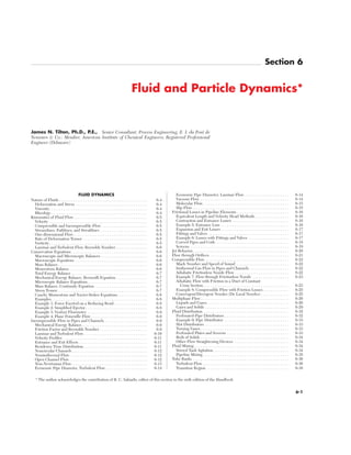
f ; (6-32)
Re ; (6-33)
For smooth pipe, the friction factor is a function only of the Reynolds
number. In rough pipe, the relative roughness e/D also affects the fric-
tion factor. Figure 6-9 plots f as a function of Re and e/D. Values of e
for various materials are given in Table 6-1. The Fanning friction fac-
tor should not be confused with the Darcy friction factor used by
Moody (Trans. ASME, 66, 671 [1944]), which is four times greater.
Using the momentum equation, the stress at the wall of the pipe may
be expressed in terms of the friction factor:
τw = f (6-34)
Laminar and Turbulent Flow Below a critical Reynolds
number of about 2,100, the flow is laminar; over the range 2,100 <
Re < 5,000 there is a transition to turbulent flow. For laminar flow, the
Hagen-Poiseuille equation
f = , Re ≤ 2,100 (6-35)
may be derived from the Navier-Stokes equation and is in excellent
agreement with experimental data. It may be rewritten in terms of
volumetric flow rate, Q = VπD2
/4, as
Q = , Re ≤ 2,100 (6-36)
π∆PD4
}
128µL
16
}
Re
ρV2
}
2
DVρ
}
µ
D∆P
}
2ρV2
L
For turbulent flow in smooth tubes, the Blasius equation gives the
friction factor accurately for a wide range of Reynolds numbers.
f = , 4,000 < Re < 105
(6-37)
The Colebrook formula (Colebrook, J. Inst. Civ. Eng. [London], 11,
133–156 [1938–39]) gives a good approximation for the f-Re-(e/D)
data for rough pipes over the entire turbulent flow range:
= −4 log 3 + 4 Re > 4,000 (6-38)
1.256
}
ReÏf
w
e
}
3.7D
1
}
Ïf
w
0.079
}
Re0.25
FIG. 6-9 Fanning Friction Factors. Reynolds number Re = DVρ/µ, where D = pipe diameter, V = velocity, ρ = fluid density, and µ = fluid vis-
cosity. (Based on Moody, Trans. ASME, 66, 671 [1944].)
TABLE 6-1 Values of Surface Roughness for Various
Materials*
Material Surface roughness ε, mm
Drawn tubing (brass, lead, glass, and the like) 0.00152
Commercial steel or wrought iron 0.0457
Asphalted cast iron 0.122
Galvanized iron 0.152
Cast iron 0.259
Wood stove 0.183–0.914
Concrete 0.305–3.05
Riveted steel 0.914–9.14
*From Moody, Trans. Am. Soc. Mech. Eng., 66, 671–684 (1944); Mech. Eng.,
69, 1005–1006 (1947). Additional values of ε for various types or conditions of
concrete wrought-iron, welded steel, riveted steel, and corrugated-metal pipes
are given in Brater and King, Handbook of Hydraulics, 6th ed., McGraw-Hill,
New York, 1976, pp. 6-12–6-13. To convert millimeters to feet, multiply by
3.281 × 10−3
.

An equation by Churchill (Chem. Eng., 84[24], 91–92 [Nov. 7, 1977])
for both smooth and rough tubes offers the advantage of being explicit
in f:
= −4 log 3 + (7/Re)0.9
4 Re > 4,000 (6-39)
In laminar flow, f is independent of e/D. In turbulent flow, the fric-
tion factor for rough pipe follows the smooth tube curve for a range of
Reynolds numbers (hydraulically smooth flow). For greater Reynolds
numbers, f deviates from the smooth pipe curve, eventually becoming
independent of Re. This region, often called complete turbulence, is
frequently encountered in commercial pipe flows. The Reynolds
number above which f becomes essentially independent of Re is
(Davies, Turbulence Phenomena, Academic, New York, 1972, p. 37)
Re = (6-40)
Roughness may also affect the transition from laminar to turbulent
flow (Schlichting).
Common pipe flow problems include calculation of pressure drop
given the flow rate (or velocity) and calculation of flow rate (or veloc-
ity) given pressure drop. When flow rate is given, the Reynolds num-
ber is first calculated to determine the flow regime, so that the
appropriate relations between f and Re (or pressure drop and velocity
or flow rate) are used. When pressure drop is given and the velocity is
unknown, the Reynolds number and flow regime cannot be immedi-
ately determined. It is necessary to assume the flow regime and then
verify by checking Re afterward. With experience, the initial guess for
the flow regime will usually prove correct. When solving Eq. (6-38)
for velocity when pressure drop is given, it is useful to note that
the right-hand side is independent of velocity since ReÏf
w =
(D3/2
/µ)Ïρ
w∆
wP
w/(
w2
wL
w)
w.
As Fig. 6-9 suggests, the friction factor is uncertain in the transition
range 2,100 < Re < 4,000 and a conservative choice should be made
for design purposes.
Velocity Profiles In laminar flow, the solution of the Navier-
Stokes equation, corresponding to the Hagen-Poiseuille equation,
gives the velocity v as a function of radial position r in a circular pipe
of radius R in terms of the average velocity V = Q/A. The parabolic
profile, with centerline velocity twice the average velocity, is shown in
Fig. 6-10.
v = 2V11 − 2 (6-41)
In turbulent flow, the velocity profile is much more blunt, with
most of the velocity gradient being in a region near the wall, described
by a universal velocity profile. It is characterized by a viscous sub-
layer, a turbulent core, and a buffer zone in between.
Viscous sublayer
u+ = y+ for y+ < 5 (6-42)
Buffer zone
u+ = 5.00 ln y+ − 3.05 for 5 < y+ < 30 (6-43)
Turbulent core
u+ = 2.5 ln y+ + 5.5 for y+ > 30 (6-44)
Here, u+ = v/u
*
is the dimensionless, time-averaged axial velocity, u
*
=
r2
}
R2
20[3.2 − 2.46 ln (e/D)]
}}}
(e/D)
0.27e
}
D
1
}
Ïf
w
Ïτw
w/ρ
w is the friction velocity and τw = fρV2
/2 is the wall stress. The
friction velocity is of the order of the root mean square velocity fluc-
tuation perpendicular to the wall in the turbulent core. The dimen-
sionless distance from the wall is y+ = yu
*
ρ/µ. The universal velocity
profile is valid in the wall region for any cross-sectional channel shape.
For incompressible flow in constant diameter circular pipes, τw =
∆P/4L where ∆P is the pressure drop in length L. In circular pipes,
Eq. (6-44) gives a surprisingly good fit to experimental results over the
entire cross section of the pipe, even though it is based on assump-
tions which are valid only near the pipe wall.
For rough pipes, the velocity profile in the turbulent core is given by
u+ = 2.5 ln y/e + 8.5 for y+ > 30 (6-45)
when the dimensionless roughness e+ = eu
*
ρ/µ is greater than 5 to 10;
for smaller e+, the velocity profile in the turbulent core is unaffected
by roughness.
For velocity profiles in the transition region, see Patel and Head
(J. Fluid Mech., 38, part 1, 181–201 [1969]) where profiles over the
range 1,500 < Re < 10,000 are reported.
Entrance and Exit Effects In the entrance region of a pipe,
some distance is required for the flow to adjust from upstream condi-
tions to the fully developed flow pattern. This distance depends on the
Reynolds number and on the flow conditions upstream. For a uniform
velocity profile at the pipe entrance, the computed length in laminar
flow required for the centerline velocity to reach 99 percent of its fully
developed value is (Dombrowski, Foumeny, Ookawara and Riza, Can.
J. Chem. Engr., 71, 472–476 [1993])
Lent /D = 0.370 exp (−0.148Re) + 0.0550Re + 0.260 (6-46)
In turbulent flow, the entrance length is about
Lent /D = 40 (6-47)
The frictional losses in the entrance region are larger than those for
the same length of fully developed flow. (See the subsection, “Fric-
tional Losses in Pipeline Elements,” following.) At the pipe exit, the
velocity profile also undergoes rearrangement, but the exit length is
much shorter than the entrance length. At low Re, it is about one pipe
radius. At Re > 100, the exit length is essentially 0.
Residence Time Distribution For laminar Newtonian pipe
flow, the cumulative residence time distribution F(θ) is given by
F(θ) = 0 for θ <
F(θ) = 1 − 1 2
2
for θ ≥ (6-48)
where F(θ) is the fraction of material which resides in the pipe for less
than time θ and θavg is the average residence time, θ = V/L.
The residence time distribution in long transfer lines may be made
narrower (more uniform) with the use of flow inverters or static
mixing elements. These devices exchange fluid between the wall
and central regions. Variations on the concept may be used to provide
effective mixing of the fluid. See Godfrey (“Static Mixers,” in Harnby,
Edwards, and Nienow, Mixing in the Process Industries, 2d ed.,
Butterworth Heinemann, Oxford, 1992); Gretta and Smith (Trans.
ASME J. Fluids Eng., 115, 255–263 [1993]); Kemblowski and Pustel-
nik (Chem. Eng. Sci., 43, 473–478 [1988]).
A theoretically derived equation for flow in helical pipe coils by
Ruthven (Chem. Eng. Sci., 26, 1113–1121 [1971]; 33, 628–629
[1978]) is given by
F(θ) = 1 − 1 23 4
2.81
for 0.5 < < 1.63 (6-49)
and was substantially confirmed by Trivedi and Vasudeva (Chem. Eng.
Sci., 29, 2291–2295 [1974]) for 0.6 < De < 6 and 0.0036 < D/Dc <
0.097 where De = ReÏD
w/D
wc
w is the Dean number and Dc is the diam-
eter of curvature of the coil. Measurements by Saxena and Nigam
(Chem. Eng. Sci., 34, 425–426 [1979]) indicate that such a distribu-
tion will hold for De > 1. The residence time distribution for helical
coils is narrower than for straight circular pipes, due to the secondary
flow which exchanges fluid between the wall and center regions.
θavg
}
θ
θavg
}
θ
1
}
4
θavg
}
2
θavg
}
θ
1
}
4
θavg
}
2
FLUID DYNAMICS 6-11
r
z v = 2V 1 –
v max = 2V
R R2
r 2
( (
FIG. 6-10 Parabolic velocity profile for laminar flow in a pipe, with average
velocity V.

In turbulent flow, axial mixing is usually described in terms of tur-
bulent diffusion or dispersion coefficients, from which cumulative
residence time distribution functions can be computed. Davies (Tur-
bulence Phenomena, Academic, New York, 1972, p. 93), gives DL =
1.01νRe0.875
for the longitudinal dispersion coefficient. Levenspiel
(Chemical Reaction Engineering, 2d ed., Wiley, New York, 1972, pp.
253–278) discusses the relations among various residence time distri-
bution functions, and the relation between dispersion coefficient and
residence time distribution.
Noncircular Channels Calculation of frictional pressure drop in
noncircular channels depends on whether the flow is laminar or turbu-
lent, and on whether the channel is full or open. For turbulent flow in
ducts running full, the hydraulic diameter DH should be substi-
tuted for D in the friction factor and Reynolds number definitions, Eqs.
(6-32) and (6-33). The hydraulic diameter is defined as four times the
channel cross-sectional area divided by the wetted perimeter.
For example, the hydraulic diameter for a circular pipe is DH = D, for
an annulus of inner diameter d and outer diameter D, DH = D − d, for a
rectangular duct of sides a, b, DH = ab/[2(a + b)]. The hydraulic radius
RH is defined as one-fourth of the hydraulic diameter.
With the hydraulic diameter subsititued for D in f and Re, Eqs.
(6-37) through (6-40) are good approximations. Note that V appearing
in f and Re is the actual average velocity V = Q/A; for noncircular
pipes; it is not Q/(πDH
2
/4). The pressure drop should be calculated
from the friction factor for noncircular pipes. Equations relating Q to
∆P and D for circular pipes may not be used for noncircular pipes
with D replaced by DH because V ≠ Q/(πDH
2
/4).
Turbulent flow in noncircular channels is generally accompanied by
secondary flows perpendicular to the axial flow direction (Schlicht-
ing). These flows may cause the pressure drop to be slightly greater
than that computed using the hydraulic diameter method. For data
on pressure drop in annuli, see Brighton and Jones (J. Basic Eng., 86,
835–842 [1964]); Okiishi and Serovy (J. Basic Eng., 89, 823–836
[1967]); and Lawn and Elliot (J. Mech. Eng. Sci., 14, 195–204 [1972]).
For rectangular ducts of large aspect ratio, Dean (J. Fluids Eng., 100,
215–233 [1978]) found that the numerator of the exponent in the Bla-
sius equation (6-37) should be increased to 0.0868. Jones (J. Fluids
Eng., 98, 173–181 [1976]) presents a method to improve the estima-
tion of friction factors for rectangular ducts using a modification of the
hydraulic diameter–based Reynolds number.
The hydraulic diameter method does not work well for laminar
flow because the shape affects the flow resistance in a way that cannot
be expressed as a function only of the ratio of cross-sectional area to
wetted perimeter. For some shapes, the Navier-Stokes equations have
been integrated to yield relations between flow rate and pressure
drop. These relations may be expressed in terms of equivalent
diameters DE defined to make the relations reduce to the second
form of the Hagen-Poiseulle equation, Eq. (6-36); that is, DE ;
(128QµL/π∆P)1/4
. Equivalent diameters are not the same as
hydraulic diameters. Equivalent diameters yield the correct rela-
tion between flow rate and pressure drop when substituted into Eq.
(6-36), but not Eq. (6-35) because V ≠ Q/(πDE/4). Equivalent diame-
ter DE is not to be used in the friction factor and Reynolds number;
f ≠ 16/Re using the equivalent diameters defined in the following. This
situation is, by arbitrary definition, opposite to that for the hydraulic
diameter DH used for turbulent flow.
Ellipse, semiaxes a and b (Lamb, Hydrodynamics, 6th ed., Dover,
New York, 1945, p. 587):
DE = 1 2
1/4
(6-50)
Rectangle, width a, height b (Owen, Trans. Am. Soc. Civ. Eng., 119,
1157–1175 [1954]):
DE = 1 2
1/4
(6-51)
a/b = 1 1.5 2 3 4 5 10 ∞
K = 28.45 20.43 17.49 15.19 14.24 13.73 12.81 12
Annulus, inner diameter D1 outer diameter D2 (Lamb, op. cit., p.
587):
128ab3
}
πK
32a3
b3
}
a2
+ b2
DE = 5(D2
2
− D1
2
)3D2
2
+ D1
2
− 46
1/4
(6-52)
For isosceles triangles and regular polygons, see Sparrow (AIChE
J., 8, 599–605 [1962]), Carlson and Irvine (J. Heat Transfer, 83,
441–444 [1961]), Cheng (Proc. Third Int. Heat Transfer Conf., New
York, 1, 64–76 [1966]), and Shih (Can. J. Chem. Eng., 45, 285–294
[1967]).
The critical Reynolds number for transition from laminar to tur-
bulent flow in noncircular channels varies with channel shape. In
rectangular ducts, 1,900 < Rec < 2,800 (Hanks and Ruo, Ind. Eng.
Chem. Fundam., 5, 558–561 [1966]). In triangular ducts, 1,600 <
Rec < 1,800 (Cope and Hanks, Ind. Eng. Chem. Fundam., 11,
106–117 [1972]; Bandopadhayay and Hinwood, J. Fluid Mech., 59,
775–783 [1973]).
Nonisothermal Flow For nonisothermal flow of liquids, the
friction factor may be increased if the liquid is being cooled or
decreased if the liquid is being heated, because of the effect of tem-
perature on viscosity near the wall. In shell and tube heat-exchanger
design, the recommended practice is to first estimate f using the bulk
mean liquid temperature over the tube length. Then, in laminar flow,
the result is divided by (µa /µw)0.23
in the case of cooling or (µa /µw)0.38
in the case of heating. For turbulent flow, f is divided by (µa /µw)0.11
in
the case of cooling or (µa /µw)0.17
in case of heating. Here, µa is the vis-
cosity at the average bulk temperature and µw is the viscosity at the
average wall temperature (Seider and Tate, Ind. Eng. Chem., 28,
1429–1435 [1936]). In the case of rough commercial pipes, rather
than heat-exchanger tubing, it is common for flow to be in the “com-
plete” turbulence regime where f is independent of Re. In such cases,
the friction factor should not be corrected for wall temperature. If the
liquid density varies with temperature, the average bulk density
should be used to calculate the pressure drop from the friction factor.
In addition, a (usually small) correction may be applied for accelera-
tion effects by adding the term G2
[(1/ρ2) − (1/ρ1)] from the mechani-
cal energy balance to the pressure drop ∆P = P1 − P2, where G is the
mass velocity. This acceleration results from small compressibility
effects associated with temperature-dependent density. Christiansen
and Gordon (AIChE J., 15, 504–507 [1969]) present equations and
charts for frictional loss in laminar nonisothermal flow of Newtonian
and non-Newtonian liquids heated or cooled with constant wall tem-
perature.
Frictional dissipation of mechanical energy can result in significant
heating of fluids, particularly for very viscous liquids in small channels.
Under adiabatic conditions, the bulk liquid temperature rise is given
by ∆T = ∆P/Cv ρ for incompressible flow through a channel of constant
cross-sectional area. For flow of polymers, this amounts to about 4°C
per 10 MPa pressure drop, while for hydrocarbon liquids it is about
6°C per 10 MPa. The temperature rise in laminar flow is highly
nonuniform, being concentrated near the pipe wall where most of the
dissipation occurs. This may result in significant viscosity reduction
near the wall, and greatly increased flow or reduced pressure drop,
and a flattened velocity profile. Compensation should generally be
made for the heat effect when ∆P exceeds 1.4 MPa (203 psi) for adia-
batic walls or 3.5 MPa (508 psi) for isothermal walls (Gerard, Steidler,
and Appeldoorn, Ind. Eng. Chem. Fundam., 4, 332–339 [1969]).
Open Channel Flow For flow in open channels, the data are
largely based on experiments with water in turbulent flow, in channels
of sufficient roughness that there is no Reynolds number effect. The
hydraulic radius approach may be used to estimate a friction factor
with which to compute friction losses. Under conditions of uniform
flow where liquid depth and cross-sectional area do not vary signifi-
cantly with position in the flow direction, there is a balance between
gravitational forces and wall stress, or equivalently between frictional
losses and potential energy change. The mechanical energy balance
reduces to lv = g(z1 − z2). In terms of the friction factor and hydraulic
diameter or hydraulic radius,
lv = = = g(z1 − z2) (6-53)
The hydraulic radius is the cross-sectional area divided by the wetted
perimeter, where the wetted perimeter does not include the free sur-
f V2
L
}
2RH
2f V2
L
}
DH
D2
2
− D1
2
}}
ln (D2 /D1)

face. Letting S = sin θ = channel slope (elevation loss per unit length
of channel, θ = angle between channel and horizontal), Eq. (6-53)
reduces to
V = !§ (6-54)
The most often used friction correlation for open channel flows is due
to Manning (Trans. Inst. Civ. Engrs. Ireland, 20, 161 [1891]) and is
equivalent to
f = (6-55)
where n is the channel roughness, with dimensions of (length)1/6
.
Table 6-2 gives roughness values for several channel types.
For gradual changes in channel cross section and liquid depth, and
for slopes less than 10°, the momentum equation for a rectangular
channel of width b and liquid depth h may be written as a differential
equation in the flow direction x.
(1 − Fr) − Fr 1 2 = S − (6-56)
For a given fixed flow rate Q = Vbh, and channel width profile b(x),
Eq. (6-56) may be integrated to determine the liquid depth profile
h(x). The dimensionless Froude number is Fr = V2
/gh. When Fr = 1,
the flow is critical, when Fr < 1, the flow is subcritical, and when
Fr > 1, the flow is supercritical. Surface disturbances move at a wave
velocity c = Ïgh
w; they cannot propagate upstream in supercritical
flows. The specific energy Esp is nearly constant.
Esp = h + (6-57)
This equation is cubic in liquid depth. Below a minimum value of Esp
there are no real positive roots; above the minimum value there are
two positive real roots. At this minimum value of Esp the flow is criti-
cal; that is, Fr = 1, V = Ïgh
w, and Esp = (3/2)h. Near critical flow condi-
tions, wave motion and sudden depth changes called hydraulic
jumps are likely. Chow (Open Channel Hydraulics, McGraw-Hill,
New York, 1959), discusses the numerous surface profile shapes
which may exist in nonuniform open channel flows.
For flow over a sharp-crested weir of width b and height L, from a
liquid depth H, the flow rate is given approximately by
Q = Cd bÏ2
wg
w(H − L)3/2
(6-58)
where Cd ≈ 0.6 is a discharge coefficient. Flow through notched weirs
is described under flow meters in Sec. 10 of the Handbook.
2
}
3
V2
}
2g
fV2
(b + 2h)
}}
2gbh
db
}
dx
h
}
b
dh
}
dx
29n2
}
RH
1/3
2gSRH
}
f
Non-Newtonian Flow For isothermal laminar flow of time-
independent non-Newtonian liquids, integration of the Cauchy
momentum equations yields the fully developed velocity profile and
flow rate–pressure drop relations. For the Bingham plastic fluid
described by Eq. (6-3), in a pipe of diameter D and a pressure drop
per unit length ∆P/L, the flow rate is given by
Q = 31 − + 4 (6-59)
where the wall stress is τw = D∆P/(4L). The velocity profile consists
of a central nondeforming plug of radius rP = 2τy /(∆P/L) and an annu-
lar deforming region. The velocity profile in the annular region is
given by
vz = 3 (R2
− r2
) − τy(R − r)4, rP ≤ r ≤ R (6-60)
where r is the radial coordinate and R is the pipe radius. The velocity
of the central, nondeforming plug is obtained by setting r = rP in Eq.
(6-60). When Q is given and Eq. (6-59) is to be solved for τw and the
pressure drop, multiple positive roots for the pressure drop may be
found. The root corresponding to τw < τy is physically unrealizable, as
it corresponds to rp > R and the pressure drop is insufficient to over-
come the yield stress.
For a power law fluid, Eq. (6-4), with constant properties K and n,
the flow rate is given by
Q = π 1 2
1/n
1 2R(1 + 3n)/n
(6-61)
and the velocity profile by
vz = 1 2
1/n
1 2[R(1 + n)/n
− r(1 + n)/n
] (6-62)
Similar relations for other non-Newtonian fluids may be found in
Govier and Aziz and in Bird, Armstrong, and Hassager (Dynamics of
Polymeric Liquids, vol. 1: Fluid Mechanics, Wiley, New York, 1977).
For steady-state laminar flow of any time-independent viscous
fluid, at average velocity V in a pipe of diameter D, the Rabinowitsch-
Mooney relations give a general relationship for the shear rate at the
pipe wall.
γ̇w = 1 2 (6-63)
where n′ is the slope of a plot of D∆P/(4L) versus 8V/D on logarithmic
coordinates,
n′ = (6-64)
By plotting capillary viscometry data this way, they can be used
directly for pressure drop design calculations, or to construct the
rheogram for the fluid. For pressure drop calculation, the flow rate
and diameter determine the velocity, from which 8V/D is calculated
and D∆P/(4L) read from the plot. For a Newtonian fluid, n′ = 1 and
the shear rate at the wall is γ̇ = 8V/D. For a power law fluid, n′ = n. To
construct a rheogram, n′ is obtained from the slope of the experimen-
tal plot at a given value of 8V/D. The shear rate at the wall is given by
Eq. (6-63) and the corresponding shear stress at the wall is τw =
D∆P/(4L) read from the plot. By varying the value of 8V/D, the shear
rate versus shear stress plot can be constructed.
The generalized approach of Metzner and Reed (AIChE J., 1, 434
[1955]) for time-independent non-Newtonian fluids defines a modi-
fied Reynolds number as
ReMR ; (6-65)
where K′ satisfies
= K′ 1 2
n′
(6-66)
With this definition, f = 16/ReMR is automatically satisfied at the value
of 8V/D where K′ and n′ are evaluated. Equation (6-66) may be
obtained by integration of Eq. (6-64) only when n′ is a constant, as, for
8V
}
D
D∆P
}
4L
Dn′
V2 − n′
ρ
}}
K′8n′ − 1
d ln [D∆P/(4L)]
}}
d ln (8V/D)
1 + 3n′
}
4n′
8V
}
D
n
}
1 + n
∆P
}
2KL
n
}
1 + 3n
∆P
}
2KL
∆P
}
4L
1
}
µ∞
τy
4
}
3τw
4
4τy
}
3τw
πD3
τw
}
32µ∞
FLUID DYNAMICS 6-13
TABLE 6-2 Average Values of n for Manning Formula,
Eq. (6-55)
Surface n, m1/6
n, ft1/6
Cast-iron pipe, fair condition 0.014 0.011
Riveted steel pipe 0.017 0.014
Vitrified sewer pipe 0.013 0.011
Concrete pipe 0.015 0.012
Wood-stave pipe 0.012 0.010
Planed-plank flume 0.012 0.010
Semicircular metal flumes, smooth 0.013 0.011
Semicircular metal flumes, corrugated 0.028 0.023
Canals and ditches
Earth, straight and uniform 0.023 0.019
Winding sluggish canals 0.025 0.021
Dredged earth channels 0.028 0.023
Natural-stream channels
Clean, straight bank, full stage 0.030 0.025
Winding, some pools and shoals 0.040 0.033
Same, but with stony sections 0.055 0.045
Sluggish reaches, very deep pools, rather weedy 0.070 0.057
SOURCE: Brater and King, Handbook of Hydraulics, 6th ed., McGraw-Hill,
New York, 1976, p. 7–22. For detailed information, see Chow, Open-Channel
Hydraulics, McGraw-Hill, New York, 1959, pp. 110–123.

example, the cases of Newtonian and power law fluids. For Newto-
nian fluids, K′ = µ and n′ = 1; for power law fluids, K′ = K[(1 + 3n)/
(4n)]n
and n′ = n. For Bingham plastics, K′ and n′ are variable, given as
a function of τw (Metzner, Ind. Eng. Chem., 49, 1429–1432 [1957]).
K = τw
1 − n′
3 4
n′
(6-67)
n′ = (6-68)
For laminar flow of power law fluids in channels of noncircular
cross section, see Schecter (AIChE J., 7, 445–448 [1961]), Wheeler
and Wissler (AIChE J., 11, 207–212 [1965]), Bird, Armstrong, and
Hassager (Dynamics of Polymeric Liquids, vol. 1: Fluid Mechanics,
Wiley, New York, 1977), and Skelland (Non-Newtonian Flow and
Heat Transfer, Wiley, New York, 1967).
Steady state, fully developed laminar flows of viscoelastic fluids in
straight, constant-diameter pipes show no effects of viscoelasticity.
The viscous component of the constitutive equation may be used to
develop the flow rate–pressure drop relations, which apply down-
stream of the entrance region after viscoelastic effects have disap-
peared. A similar situation exists for time-dependent fluids.
The transition to turbulent flow begins at ReMR in the range of
2,000 to 2,500 (Metzner and Reed, AIChE J., 1, 434 [1955]). For
Bingham plastic materials, K′ and n′ must be evaluated for the τw con-
dition in question in order to determine ReMR and establish whether
the flow is laminar. An alternative method for Bingham plastics is by
Hanks (Hanks, AIChE J., 9, 306 [1963]; 14, 691 [1968]; Hanks and
Pratt, Soc. Petrol. Engrs. J., 7, 342 [1967]; and Govier and Aziz, pp.
213–215). The transition from laminar to turbulent flow is influenced
by viscoelastic properties (Metzner and Park, J. Fluid Mech., 20, 291
[1964]) with the critical value of ReMR increased to beyond 10,000 for
some materials.
For turbulent flow of non-Newtonian fluids, the design chart of
Dodge and Metzner (AIChE J., 5, 189 [1959]), Fig. 6-11, is most
widely used. For Bingham plastic materials in turbulent flow, it is gen-
erally assumed that stresses greatly exceed the yield stress, so that the
friction factor–Reynolds number relationship for Newtonian fluids
applies, with µ∞ substituted for µ. This is equivalent to setting n′ = 1
and τy /τw = 0 in the Dodge-Metzner method, so that ReMR = DVρ/µ∞.
Wilson and Thomas (Can. J. Chem. Eng., 63, 539–546 [1985]) give
friction factor equations for turbulent flow of power law fluids and
Bingham plastic fluids.
Power law fluids:
= + 8.2 + 1.77 ln 1 2 (6-69)
1 + n
}
2
1 − n
}
1 + n
1
}
ÏfN
w
1
}
Ïf
w
1 − 4τy /(3τw) + (τy /τw)4
/3
}}}
1 − (τy /τw)4
µ∞
}}}
1 − 4τy /3τw + (τy /τw)4
/3
where fN is the friction factor for Newtonian fluid evaluated at Re =
DVρ/µeff where the effective viscosity is
µeff = K1 2
n − 1
1 2
n − 1
(6-70)
Bingham fluids:
= + 1.77 ln 1 2+ ξ(10 + 0.884ξ) (6-71)
where fN is evaluated at Re = DVρ/µ∞ and ξ = τy /τw. Iteration is
required to use this equation since τw = fρV2
/2.
Drag reduction in turbulent flow can be achieved by adding solu-
ble high molecular weight polymers in extremely low concentration to
Newtonian liquids. The reduction in friction is generally believed to
be associated with the viscoelastic nature of the solutions effective in
the wall region. For a given polymer, there is a minimum molecular
weight necessary to initiate drag reduction at a given flow rate, and a
critical concentration above which drag reduction will not occur (Kim,
Little and Ting, J. Colloid Interface Sci., 47, 530–535 [1974]). Drag
reduction is reviewed by Hoyt (J. Basic Eng., 94, 258–285 [1972]);
Little, et al. (Ind. Eng. Chem. Fundam., 14, 283–296 [1975]) and Virk
(AIChE J., 21, 625–656 [1975]). At maximum possible drag reduction
in smooth pipes,
= −19 log 1 2 (6-72)
or, approximately, f = (6-73)
for 4,000 < Re < 40,000. The actual drag reduction depends on the
polymer system. For further details, see Virk (ibid.).
Economic Pipe Diameter, Turbulent Flow The economic
optimum pipe diameter may be computed so that the last increment
of investment reduces the operating cost enough to produce the
required minimum return on investment. For long cross-country
pipelines, alloy pipes of appreciable length and complexity, or pipe-
lines with control valves, detailed analyses of investment and operat-
ing costs should be made. Peters and Timmerhaus (Plant Design and
Economics for Chemical Engineers, 4th ed., McGraw-Hill, New York,
1991) provide a detailed method for determining the economic opti-
mum size. For pipelines of the lengths usually encountered in chemi-
cal plants and petroleum refineries, simplified selection charts are
often adequate. In many cases there is an economic optimum velocity
that is nearly independent of diameter, which may be used to estimate
the economic diameter from the flow rate. For low-viscosity liquids in
schedule 40 steel pipe, economic optimum velocity is typically in the
range of 1.8 to 2.4 m/s (5.9 to 7.9 ft/s). For gases with density ranging
from 0.2 to 20 kg/m3
(0.013 to 1.25 lbm/ft3
), the economic optimum
velocity is about 40 m/s to 9 m/s (131 to 30 ft/s). Charts and rough
guidelines for economic optimum size do not apply to multiphase
flows.
Economic Pipe Diameter, Laminar Flow Pipelines for the
transport of high-viscosity liquids are seldom designed purely on the
basis of economics. More often, the size is dictated by operability con-
siderations such as available pressure drop, shear rate, or residence
time distribution. Peters and Timmerhaus (ibid., Chap. 10) provide an
economic pipe diameter chart for laminar flow. For non-Newtonian
fluids, see Skelland (Non-Newtonian Flow and Heat Transfer, Chap.
7, Wiley, New York, 1967).
Vacuum Flow When gas flows under high vacuum conditions or
through very small openings, the continuum hypothesis is no longer
appropriate if the channel dimension is not very large compared to the
mean free path of the gas. When the mean free path is comparable to
the channel dimension, flow is dominated by collisions of molecules
with the wall, rather than by collisions between molecules. An approx-
imate expression based on Brown, et al. (J. Appl. Phys., 17, 802–813
[1946]) for the mean free path is
λ = 1 2!§ (6-74)
8RT
}
πMw
2µ
}
p
0.58
}
Re0.58
50.73
}
ReÏf
w
1
}
Ïf
w
(1 − ξ)2
}
1 + ξ
1
}
ÏfN
w
1
}
Ïf
w
8V
}
D
3n + 1
}
4n
FIG. 6-11 Fanning friction factor for non-Newtonian flow. (From Dodge and
Metzner, Am. Inst. Chem. Eng. J., 5, 189 [1959]).

The Knudsen number Kn is the ratio of the mean free path to the
channel dimension. For pipe flow, Kn = λ/D. Molecular flow is char-
acterized by Kn > 1.0; continuum viscous (laminar or turbulent) flow
is characterized by Kn < 0.01. Transition or slip flow applies over the
range 0.01 < Kn < 1.0.
Vacuum flow is usually described with flow variables different from
those used for normal pressures, which often leads to confusion.
Pumping speed S is the actual volumetric flow rate of gas through a
flow cross section. Throughput Q is the product of pumping speed
and absolute pressure. In the SI system, Q has units of Pa ⋅ m3
/s.
Q = Sp (6-75)
The mass flow rate w is related to the throughput using the ideal gas law.
w = Q (6-76)
Throughput is therefore proportional to mass flow rate. For a given
mass flow rate, throughput is independent of pressure. The relation
between throughput and pressure drop ∆p = p1 − p2 across a flow ele-
ment is written in terms of the conductance C. Resistance is the
reciprocal of conductance. Conductance has dimensions of volume
per time.
Q = C∆p (6-77)
The conductance of a series of flow elements is given by
= + + + ⋅⋅⋅ (6-78)
while for elements in parallel,
C = C1 + C2 + C3 + ⋅⋅⋅ (6-79)
For a vacuum pump of speed Sp withdrawing from a vacuum vessel
through a connecting line of conductance C, the pumping speed at
the vessel is
S = (6-80)
Molecular Flow Under molecular flow conditions, conductance
is independent of pressure. It is proportional to ÏT
w/M
ww
w, with the pro-
portionality constant a function of geometry. For fully developed pipe
flow,
C = !§ (6-81)
For an orifice of area A,
C = 0.40A!§ (6-82)
Conductance equations for several other geometries are given by
Ryans and Roper (Process Vacuum System Design and Operation,
Chap. 2, McGraw-Hill, New York, 1986). For a circular annulus of
outer and inner diameters D1 and D2 and length L, the method of
Guthrie and Wakerling (Vacuum Equipment and Techniques,
McGraw-Hill, New York, 1949) may be written
C = 0.42K !§ (6-83)
where K is a dimensionless constant with values given in Table 6-3.
For a short pipe of circular cross section, the conductance as calcu-
lated for an orifice from Eq. (6-82) is multiplied by a correction factor
K which may be approximated as (Kennard, Kinetic Theory of Gases,
McGraw-Hill, New York, 1938, pp. 306–308)
RT
}
Mw
(D1 − D2)2
(D1 + D2)
}}}
L
RT
}
Mw
RT
}
Mw
πD3
}
8L
SpC
}
Sp + C
1
}
C3
1
}
C2
1
}
C1
1
}
C
Mw
}
RT
K = for 0 ≤ L/D ≤ 0.75 (6-84)
K = for L/D > 0.75 (6-85)
For L/D > 100, the error in neglecting the end correction by using the
fully developed pipe flow equation (6-81) is less than 2 percent. For
rectangular channels, see Normand (Ind. Eng. Chem., 40, 783–787
[1948]).
Yu and Sparrow (J. Basic Eng., 70, 405–410 [1970]) give a theoret-
ically derived chart for slot seals with or without a sheet located in or
passing through the seal, giving mass flow rate as a function of the
ratio of seal plate thickness to gap opening.
Slip Flow In the transition region between molecular flow and
continuum viscous flow, the conductance for fully developed pipe
flow is most easily obtained by the method of Brown, et al. (J. Appl.
Phys., 17, 802–813 [1946]), which uses the parameter
X = !§1 2= 1 2!§ (6-86)
where pm is the arithmetic mean absolute pressure. A correction fac-
tor F, read from Fig. 6-12 as a function of X, is applied to the conduc-
tance for viscous flow.
C = F (6-87)
For slip flow through square channels, see Milligan and Wilker-
son (J. Eng. Ind., 95, 370–372 [1973]). For slip flow through annuli,
see Maegley and Berman (Phys. Fluids, 15, 780–785 [1972]).
The pump-down time θ for evacuating a vessel in the absence of
air in-leakage is given approximately by
θ = 1 2ln 1 2 (6-88)
where Vt = volume of vessel plus volume of piping between vessel and
pump; S0 = system speed as given by Eq. (6-80), assumed independent
of pressure; p1 = initial vessel pressure; p2 = final vessel pressure; and
p0 = lowest pump intake pressure attainable with the pump in ques-
tion. See Dushman and Lafferty (Scientific Foundations of Vacuum
Technique, 2d ed., Wiley, New York, 1962).
The amount of inerts which has to be removed by a pumping sys-
tem after the pump-down stage depends on the in-leakage of air at the
various fittings, connections, and so on. Air leakage is often correlated
with system volume and pressure, but this approach introduces uncer-
p1 − p0
}
p2 − p0
Vt
}
S0
πD4
pm
}
128µL
RT
}
M
2µ
}
pmD
λ
}
D
8
}
π
1 + 0.8(L/D)
}}}
1 + 1.90(L/D) + 0.6(L/D)2
1
}}
1 + (L/D)
FLUID DYNAMICS 6-15
TABLE 6-3 Constants for Circular Annuli
D2 /D1 K D2 /D1 K
0 1.00 0.707 1.254
0.259 1.072 0.866 1.430
0.500 1.154 0.966 1.675
FIG. 6-12 Correction factor for Poiseuille’s equation at low pressures. Curve
A: experimental curve for glass capillaries and smooth metal tubes. (From
Brown, et al., J. Appl. Phys., 17, 802 [1946].) Curve B: experimental curve for
iron pipe (From Riggle, Courtesy of E. I. du Pont de Nemours & Co.)

Perry’s Chemical Engineers’ Handbook 7ma Ed Chap 06

Perry’s Chemical Engineers’ Handbook 7ma Ed Chap 06

Recommended

Recommended

More Related Content

What's hot

What's hot (20)

Similar to Perry’s Chemical Engineers’ Handbook 7ma Ed Chap 06

Similar to Perry’s Chemical Engineers’ Handbook 7ma Ed Chap 06 (20)

More from Grey Enterprise Holdings, Inc.

More from Grey Enterprise Holdings, Inc. (14)

Recently uploaded

Recently uploaded (20)

Perry’s Chemical Engineers’ Handbook 7ma Ed Chap 06