SlideShare a Scribd company logo
1 of 668
Download to read offline
CalculiX CrunchiX USER’S MANUAL version
2.15
Guido Dhondt
December 15, 2018
Contents
1 Introduction. 10
2 How to perform CalculiX calculations in parallel 11
3 Units 13
4 Golden rules 15
5 Simple example problems 17
5.1 Cantilever beam . . . . . . . . . . . . . . . . . . . . . . . . . . . 17
5.2 Frequency calculation of a beam loaded by compressive forces . . 24
5.3 Frequency calculation of a rotating disk on a slender shaft . . . . 26
5.4 Thermal calculation of a furnace . . . . . . . . . . . . . . . . . . 32
5.5 Seepage under a dam . . . . . . . . . . . . . . . . . . . . . . . . . 37
5.6 Capacitance of a cylindrical capacitor . . . . . . . . . . . . . . . 39
5.7 Hydraulic pipe system . . . . . . . . . . . . . . . . . . . . . . . . 43
5.8 Lid-driven cavity . . . . . . . . . . . . . . . . . . . . . . . . . . . 48
5.9 Transient laminar incompressible Couette problem . . . . . . . . 52
5.10 Stationary laminar inviscid compressible airfoil flow . . . . . . . 54
5.11 Stationary laminar viscous compressible airfoil flow . . . . . . . . 59
5.12 Channel with hydraulic jump . . . . . . . . . . . . . . . . . . . . 60
5.13 Cantilever beam using beam elements . . . . . . . . . . . . . . . 63
5.14 Reinforced concrete cantilever beam . . . . . . . . . . . . . . . . 70
5.15 Wrinkling of a thin sheet . . . . . . . . . . . . . . . . . . . . . . . 72
5.16 Optimization of a simply supported beam . . . . . . . . . . . . . 75
5.17 Mesh refinement of a curved cantilever beam . . . . . . . . . . . 81
6 Theory 86
6.1 Node Types . . . . . . . . . . . . . . . . . . . . . . . . . . . . . . 87
6.2 Element Types . . . . . . . . . . . . . . . . . . . . . . . . . . . . 88
6.2.1 Eight-node brick element (C3D8 and F3D8) . . . . . . . . 88
1
2 CONTENTS
6.2.2 C3D8R . . . . . . . . . . . . . . . . . . . . . . . . . . . . 90
6.2.3 Incompatible mode eight-node brick element (C3D8I) . . 91
6.2.4 Twenty-node brick element (C3D20) . . . . . . . . . . . . 91
6.2.5 C3D20R . . . . . . . . . . . . . . . . . . . . . . . . . . . . 92
6.2.6 Four-node tetrahedral element (C3D4 and F3D4) . . . . . 93
6.2.7 Ten-node tetrahedral element (C3D10) . . . . . . . . . . . 93
6.2.8 Modified ten-node tetrahedral element (C3D10T) . . . . . 93
6.2.9 Six-node wedge element (C3D6 and F3D6) . . . . . . . . 96
6.2.10 Fifteen-node wedge element (C3D15) . . . . . . . . . . . . 96
6.2.11 Three-node shell element (S3) . . . . . . . . . . . . . . . . 98
6.2.12 Four-node shell element (S4 and S4R) . . . . . . . . . . . 98
6.2.13 Six-node shell element (S6) . . . . . . . . . . . . . . . . . 98
6.2.14 Eight-node shell element (S8 and S8R) . . . . . . . . . . . 98
6.2.15 Three-node membrane element (M3D3) . . . . . . . . . . 107
6.2.16 Four-node membrane element (M3D4 and M3D4R) . . . . 107
6.2.17 Six-node membrane element (M3D6) . . . . . . . . . . . . 107
6.2.18 Eight-node membrane element (M3D8 and M3D8R) . . . 107
6.2.19 Three-node plane stress element (CPS3) . . . . . . . . . . 107
6.2.20 Four-node plane stress element (CPS4 and CPS4R) . . . 107
6.2.21 Six-node plane stress element (CPS6) . . . . . . . . . . . 108
6.2.22 Eight-node plane stress element (CPS8 and CPS8R) . . . 108
6.2.23 Three-node plane strain element (CPE3) . . . . . . . . . . 110
6.2.24 Four-node plane strain element (CPE4 and CPE4R) . . . 110
6.2.25 Six-node plane strain element (CPE6) . . . . . . . . . . . 110
6.2.26 Eight-node plane strain element (CPE8 and CPE8R) . . . 110
6.2.27 Three-node axisymmetric element (CAX3) . . . . . . . . 110
6.2.28 Four-node axisymmetric element (CAX4 and CAX4R) . . 111
6.2.29 Six-node axisymmetric element (CAX6) . . . . . . . . . . 111
6.2.30 Eight-node axisymmetric element (CAX8 and CAX8R) . 111
6.2.31 Two-node 2D beam element (B21) . . . . . . . . . . . . . 113
6.2.32 Two-node 3D beam element (B31 and B31R) . . . . . . . 113
6.2.33 Three-node 3D beam element (B32 and B32R) . . . . . . 113
6.2.34 Two-node 2D truss element (T2D2) . . . . . . . . . . . . 119
6.2.35 Two-node 3D truss element (T3D2) . . . . . . . . . . . . 119
6.2.36 Three-node 3D truss element (T3D3) . . . . . . . . . . . . 121
6.2.37 Three-node network element (D) . . . . . . . . . . . . . . 121
6.2.38 Two-node unidirectional gap element (GAPUNI) . . . . . 122
6.2.39 Two-node 3-dimensional dashpot (DASHPOTA) . . . . . 122
6.2.40 One-node 3-dimensional spring (SPRING1) . . . . . . . . 123
6.2.41 Two-node 3-dimensional spring (SPRING2) . . . . . . . . 123
6.2.42 Two-node 3-dimensional spring (SPRINGA) . . . . . . . . 124
6.2.43 One-node coupling element (DCOUP3D) . . . . . . . . . 124
6.2.44 One-node mass element (MASS) . . . . . . . . . . . . . . 124
6.2.45 User Element (Uxxxx) . . . . . . . . . . . . . . . . . . . . 124
6.3 Beam Section Types . . . . . . . . . . . . . . . . . . . . . . . . . 125
6.3.1 Pipe . . . . . . . . . . . . . . . . . . . . . . . . . . . . . . 126
CONTENTS 3
6.3.2 Box . . . . . . . . . . . . . . . . . . . . . . . . . . . . . . 126
6.3.3 General . . . . . . . . . . . . . . . . . . . . . . . . . . . . 128
6.4 Fluid Section Types: Gases . . . . . . . . . . . . . . . . . . . . . 129
6.4.1 Orifice . . . . . . . . . . . . . . . . . . . . . . . . . . . . . 133
6.4.2 Bleed Tapping . . . . . . . . . . . . . . . . . . . . . . . . 136
6.4.3 Preswirl Nozzle . . . . . . . . . . . . . . . . . . . . . . . . 137
6.4.4 Straight and Stepped Labyrinth . . . . . . . . . . . . . . . 138
6.4.5 Characteristic . . . . . . . . . . . . . . . . . . . . . . . . . 142
6.4.6 Carbon Seal . . . . . . . . . . . . . . . . . . . . . . . . . . 143
6.4.7 Gas Pipe (Fanno) . . . . . . . . . . . . . . . . . . . . . . 145
6.4.8 Restrictor, Long Orifice . . . . . . . . . . . . . . . . . . . 151
6.4.9 Restrictor, Enlargement . . . . . . . . . . . . . . . . . . . 154
6.4.10 Restrictor, Contraction . . . . . . . . . . . . . . . . . . . 155
6.4.11 Restrictor, Bend . . . . . . . . . . . . . . . . . . . . . . . 156
6.4.12 Restrictor, Wall Orifice . . . . . . . . . . . . . . . . . . . 157
6.4.13 Restrictor, Entrance . . . . . . . . . . . . . . . . . . . . . 159
6.4.14 Restrictor, Exit . . . . . . . . . . . . . . . . . . . . . . . . 160
6.4.15 Restrictor, User . . . . . . . . . . . . . . . . . . . . . . . . 160
6.4.16 Branch, Joint . . . . . . . . . . . . . . . . . . . . . . . . . 161
6.4.17 Branch, Split . . . . . . . . . . . . . . . . . . . . . . . . . 164
6.4.18 Cross, Split . . . . . . . . . . . . . . . . . . . . . . . . . . 168
6.4.19 Vortex . . . . . . . . . . . . . . . . . . . . . . . . . . . . . 169
6.4.20 Möhring . . . . . . . . . . . . . . . . . . . . . . . . . . . . 173
6.4.21 Change absolute/relative system . . . . . . . . . . . . . . 174
6.4.22 In/Out . . . . . . . . . . . . . . . . . . . . . . . . . . . . 177
6.4.23 Mass Flow Percent . . . . . . . . . . . . . . . . . . . . . . 177
6.4.24 Network User Element . . . . . . . . . . . . . . . . . . . . 178
6.5 Fluid Section Types: Liquids . . . . . . . . . . . . . . . . . . . . 179
6.5.1 Pipe, Manning . . . . . . . . . . . . . . . . . . . . . . . . 179
6.5.2 Pipe, White-Colebrook . . . . . . . . . . . . . . . . . . . . 180
6.5.3 Pipe, Sudden Enlargement . . . . . . . . . . . . . . . . . 182
6.5.4 Pipe, Sudden Contraction . . . . . . . . . . . . . . . . . . 183
6.5.5 Pipe, Entrance . . . . . . . . . . . . . . . . . . . . . . . . 183
6.5.6 Pipe, Diaphragm . . . . . . . . . . . . . . . . . . . . . . . 184
6.5.7 Pipe, Bend . . . . . . . . . . . . . . . . . . . . . . . . . . 185
6.5.8 Pipe, Gate Valve . . . . . . . . . . . . . . . . . . . . . . . 186
6.5.9 Pump . . . . . . . . . . . . . . . . . . . . . . . . . . . . . 187
6.5.10 In/Out . . . . . . . . . . . . . . . . . . . . . . . . . . . . 189
6.6 Fluid Section Types: Open Channels . . . . . . . . . . . . . . . . 189
6.6.1 Straight Channel . . . . . . . . . . . . . . . . . . . . . . . 190
6.6.2 Sluice Gate . . . . . . . . . . . . . . . . . . . . . . . . . . 190
6.6.3 Sluice Opening . . . . . . . . . . . . . . . . . . . . . . . . 192
6.6.4 Weir Crest . . . . . . . . . . . . . . . . . . . . . . . . . . 192
6.6.5 Weir slope . . . . . . . . . . . . . . . . . . . . . . . . . . . 193
6.6.6 Discontinuous Slope . . . . . . . . . . . . . . . . . . . . . 194
6.6.7 Discontinuous Opening . . . . . . . . . . . . . . . . . . . 195
4 CONTENTS
6.6.8 Reservoir . . . . . . . . . . . . . . . . . . . . . . . . . . . 196
6.6.9 Contraction . . . . . . . . . . . . . . . . . . . . . . . . . . 196
6.6.10 Enlargement . . . . . . . . . . . . . . . . . . . . . . . . . 198
6.6.11 Drop . . . . . . . . . . . . . . . . . . . . . . . . . . . . . . 198
6.6.12 Step . . . . . . . . . . . . . . . . . . . . . . . . . . . . . . 199
6.6.13 In/Out . . . . . . . . . . . . . . . . . . . . . . . . . . . . 199
6.7 Boundary conditions . . . . . . . . . . . . . . . . . . . . . . . . . 199
6.7.1 Single point constraints (SPC) . . . . . . . . . . . . . . . 199
6.7.2 Multiple point constraints (MPC) . . . . . . . . . . . . . 200
6.7.3 Kinematic and Distributing Coupling . . . . . . . . . . . 200
6.7.4 Mathematical description of a knot . . . . . . . . . . . . . 201
6.7.5 Node-to-Face Penalty Contact . . . . . . . . . . . . . . . 204
6.7.6 Face-to-Face Penalty Contact . . . . . . . . . . . . . . . . 220
6.8 Materials . . . . . . . . . . . . . . . . . . . . . . . . . . . . . . . 226
6.8.1 Linear elastic materials . . . . . . . . . . . . . . . . . . . 226
6.8.2 Linear elastic materials for large strains (Ciarlet model) . 226
6.8.3 Linear elastic materials for rotation-insensitive small strains228
6.8.4 Ideal gas for quasi-static calculations . . . . . . . . . . . . 229
6.8.5 Hyperelastic and hyperfoam materials . . . . . . . . . . . 229
6.8.6 Deformation plasticity . . . . . . . . . . . . . . . . . . . . 230
6.8.7 Incremental (visco)plasticity: multiplicative decomposition 230
6.8.8 Incremental (visco)plasticity: additive decomposition . . . 232
6.8.9 Tension-only and compression-only materials. . . . . . . . 232
6.8.10 Fiber reinforced materials. . . . . . . . . . . . . . . . . . . 233
6.8.11 The Cailletaud single crystal model. . . . . . . . . . . . . 235
6.8.12 The Cailletaud single crystal creep model. . . . . . . . . . 238
6.8.13 Elastic anisotropy with isotropic viscoplasticity. . . . . . . 240
6.8.14 Elastic anisotropy with isotropic creep defined by a creep user subroutine.243
6.8.15 User materials . . . . . . . . . . . . . . . . . . . . . . . . 245
6.9 Types of analysis . . . . . . . . . . . . . . . . . . . . . . . . . . . 245
6.9.1 Static analysis . . . . . . . . . . . . . . . . . . . . . . . . 245
6.9.2 Frequency analysis . . . . . . . . . . . . . . . . . . . . . . 246
6.9.3 Complex frequency analysis . . . . . . . . . . . . . . . . . 250
6.9.4 Buckling analysis . . . . . . . . . . . . . . . . . . . . . . . 251
6.9.5 Modal dynamic analysis . . . . . . . . . . . . . . . . . . . 252
6.9.6 Steady state dynamics . . . . . . . . . . . . . . . . . . . . 254
6.9.7 Direct integration dynamic analysis . . . . . . . . . . . . 256
6.9.8 Heat transfer . . . . . . . . . . . . . . . . . . . . . . . . . 256
6.9.9 Acoustics . . . . . . . . . . . . . . . . . . . . . . . . . . . 258
6.9.10 Shallow water motion . . . . . . . . . . . . . . . . . . . . 259
6.9.11 Hydrodynamic lubrication . . . . . . . . . . . . . . . . . . 260
6.9.12 Irrotational incompressible inviscid flow . . . . . . . . . . 261
6.9.13 Electrostatics . . . . . . . . . . . . . . . . . . . . . . . . . 262
6.9.14 Stationary groundwater flow . . . . . . . . . . . . . . . . 263
6.9.15 Diffusion mass transfer in a stationary medium . . . . . . 265
6.9.16 Aerodynamic Networks . . . . . . . . . . . . . . . . . . . 267
CONTENTS 5
6.9.17 Hydraulic Networks . . . . . . . . . . . . . . . . . . . . . 269
6.9.18 Turbulent Flow in Open Channels . . . . . . . . . . . . . 271
6.9.19 Three-dimensional Navier-Stokes Calculations . . . . . . 273
6.9.20 Substructure Generation . . . . . . . . . . . . . . . . . . 273
6.9.21 Electromagnetism . . . . . . . . . . . . . . . . . . . . . . 274
6.9.22 Sensitivity . . . . . . . . . . . . . . . . . . . . . . . . . . 286
6.9.23 Green functions . . . . . . . . . . . . . . . . . . . . . . . . 290
6.10 Convergence criteria . . . . . . . . . . . . . . . . . . . . . . . . . 291
6.10.1 Thermomechanical iterations . . . . . . . . . . . . . . . . 291
6.10.2 Contact . . . . . . . . . . . . . . . . . . . . . . . . . . . . 294
6.10.3 Line search . . . . . . . . . . . . . . . . . . . . . . . . . . 296
6.10.4 Network iterations . . . . . . . . . . . . . . . . . . . . . . 297
6.10.5 Implicit dynamics . . . . . . . . . . . . . . . . . . . . . . 298
6.11 Loading . . . . . . . . . . . . . . . . . . . . . . . . . . . . . . . . 300
6.11.1 Point loads . . . . . . . . . . . . . . . . . . . . . . . . . . 300
6.11.2 Facial distributed loading . . . . . . . . . . . . . . . . . . 300
6.11.3 Centrifugal distributed loading . . . . . . . . . . . . . . . 303
6.11.4 Gravity distributed loading . . . . . . . . . . . . . . . . . 304
6.11.5 Forces obtained by selecting RF . . . . . . . . . . . . . . 304
6.11.6 Temperature loading in a mechanical analysis . . . . . . . 307
6.11.7 Initial(residual) stresses . . . . . . . . . . . . . . . . . . . 307
6.11.8 Concentrated heat flux . . . . . . . . . . . . . . . . . . . . 307
6.11.9 Distributed heat flux . . . . . . . . . . . . . . . . . . . . . 307
6.11.10Convective heat flux . . . . . . . . . . . . . . . . . . . . . 307
6.11.11Radiative heat flux . . . . . . . . . . . . . . . . . . . . . . 308
6.12 Error estimators . . . . . . . . . . . . . . . . . . . . . . . . . . . 308
6.12.1 Zienkiewicz-Zhu error estimator . . . . . . . . . . . . . . . 308
6.12.2 Gradient error estimator . . . . . . . . . . . . . . . . . . . 309
6.13 Output variables . . . . . . . . . . . . . . . . . . . . . . . . . . . 310
7 Input deck format 312
7.1 *AMPLITUDE . . . . . . . . . . . . . . . . . . . . . . . . . . . . 313
7.2 *BASE MOTION . . . . . . . . . . . . . . . . . . . . . . . . . . . 315
7.3 *BEAM SECTION . . . . . . . . . . . . . . . . . . . . . . . . . . 316
7.4 *BOUNDARY . . . . . . . . . . . . . . . . . . . . . . . . . . . . 318
7.4.1 Homogeneous Conditions . . . . . . . . . . . . . . . . . . 320
7.4.2 Inhomogeneous Conditions . . . . . . . . . . . . . . . . . 321
7.4.3 Submodel . . . . . . . . . . . . . . . . . . . . . . . . . . . 322
7.5 *BOUNDARYF . . . . . . . . . . . . . . . . . . . . . . . . . . . . 322
7.6 *BUCKLE . . . . . . . . . . . . . . . . . . . . . . . . . . . . . . 324
7.7 *CFD . . . . . . . . . . . . . . . . . . . . . . . . . . . . . . . . . 325
7.8 *CFLUX . . . . . . . . . . . . . . . . . . . . . . . . . . . . . . . 327
7.9 *CHANGE FRICTION . . . . . . . . . . . . . . . . . . . . . . . 328
7.10 *CHANGE MATERIAL . . . . . . . . . . . . . . . . . . . . . . . 329
7.11 *CHANGE PLASTIC . . . . . . . . . . . . . . . . . . . . . . . . 329
7.12 *CHANGE SURFACE BEHAVIOR . . . . . . . . . . . . . . . . 330
6 CONTENTS
7.13 *CHANGE SOLID SECTION . . . . . . . . . . . . . . . . . . . . 331
7.14 *CLEARANCE . . . . . . . . . . . . . . . . . . . . . . . . . . . . 332
7.15 *CLOAD . . . . . . . . . . . . . . . . . . . . . . . . . . . . . . . 332
7.16 *COMPLEX FREQUENCY . . . . . . . . . . . . . . . . . . . . . 335
7.17 *CONDUCTIVITY . . . . . . . . . . . . . . . . . . . . . . . . . 336
7.18 *CONSTRAINT . . . . . . . . . . . . . . . . . . . . . . . . . . . 337
7.19 *CONTACT DAMPING . . . . . . . . . . . . . . . . . . . . . . . 339
7.20 *CONTACT FILE . . . . . . . . . . . . . . . . . . . . . . . . . . 340
7.21 *CONTACT OUTPUT . . . . . . . . . . . . . . . . . . . . . . . 342
7.22 *CONTACT PAIR . . . . . . . . . . . . . . . . . . . . . . . . . . 343
7.23 *CONTACT PRINT . . . . . . . . . . . . . . . . . . . . . . . . . 344
7.24 *CONTROLS . . . . . . . . . . . . . . . . . . . . . . . . . . . . . 346
7.25 *COUPLED TEMPERATURE-DISPLACEMENT . . . . . . . . 351
7.26 *COUPLING . . . . . . . . . . . . . . . . . . . . . . . . . . . . . 353
7.27 *CREEP . . . . . . . . . . . . . . . . . . . . . . . . . . . . . . . 354
7.28 *CYCLIC HARDENING . . . . . . . . . . . . . . . . . . . . . . 355
7.29 *CYCLIC SYMMETRY MODEL . . . . . . . . . . . . . . . . . . 356
7.30 *DAMPING . . . . . . . . . . . . . . . . . . . . . . . . . . . . . . 358
7.31 *DASHPOT . . . . . . . . . . . . . . . . . . . . . . . . . . . . . . 359
7.32 *DEFORMATION PLASTICITY . . . . . . . . . . . . . . . . . . 361
7.33 *DENSITY . . . . . . . . . . . . . . . . . . . . . . . . . . . . . . 361
7.34 *DEPVAR . . . . . . . . . . . . . . . . . . . . . . . . . . . . . . . 362
7.35 *DESIGN VARIABLES . . . . . . . . . . . . . . . . . . . . . . . 363
7.36 *DFLUX . . . . . . . . . . . . . . . . . . . . . . . . . . . . . . . 363
7.37 *DISTRIBUTING . . . . . . . . . . . . . . . . . . . . . . . . . . 367
7.38 *DISTRIBUTING COUPLING . . . . . . . . . . . . . . . . . . . 369
7.39 *DLOAD . . . . . . . . . . . . . . . . . . . . . . . . . . . . . . . 371
7.40 *DSLOAD . . . . . . . . . . . . . . . . . . . . . . . . . . . . . . . 376
7.41 *DYNAMIC . . . . . . . . . . . . . . . . . . . . . . . . . . . . . . 378
7.42 *ELASTIC . . . . . . . . . . . . . . . . . . . . . . . . . . . . . . 380
7.43 *ELECTRICAL CONDUCTIVITY . . . . . . . . . . . . . . . . . 383
7.44 *ELECTROMAGNETICS . . . . . . . . . . . . . . . . . . . . . . 384
7.45 *ELEMENT . . . . . . . . . . . . . . . . . . . . . . . . . . . . . 386
7.46 *ELEMENT OUTPUT . . . . . . . . . . . . . . . . . . . . . . . 388
7.47 *EL FILE . . . . . . . . . . . . . . . . . . . . . . . . . . . . . . . 389
7.48 *EL PRINT . . . . . . . . . . . . . . . . . . . . . . . . . . . . . . 393
7.49 *ELSET . . . . . . . . . . . . . . . . . . . . . . . . . . . . . . . . 396
7.50 *END STEP . . . . . . . . . . . . . . . . . . . . . . . . . . . . . 397
7.51 *EQUATION . . . . . . . . . . . . . . . . . . . . . . . . . . . . . 397
7.52 *EXPANSION . . . . . . . . . . . . . . . . . . . . . . . . . . . . 399
7.53 *FILM . . . . . . . . . . . . . . . . . . . . . . . . . . . . . . . . . 401
7.54 *FILTER . . . . . . . . . . . . . . . . . . . . . . . . . . . . . . . 405
7.55 *FLUID CONSTANTS . . . . . . . . . . . . . . . . . . . . . . . 406
7.56 *FLUID SECTION . . . . . . . . . . . . . . . . . . . . . . . . . . 407
7.57 *FREQUENCY . . . . . . . . . . . . . . . . . . . . . . . . . . . . 408
7.58 *FRICTION . . . . . . . . . . . . . . . . . . . . . . . . . . . . . 410
CONTENTS 7
7.59 *GAP . . . . . . . . . . . . . . . . . . . . . . . . . . . . . . . . . 411
7.60 *GAP CONDUCTANCE . . . . . . . . . . . . . . . . . . . . . . 412
7.61 *GAP HEAT GENERATION . . . . . . . . . . . . . . . . . . . . 413
7.62 *GREEN . . . . . . . . . . . . . . . . . . . . . . . . . . . . . . . 414
7.63 *HEADING . . . . . . . . . . . . . . . . . . . . . . . . . . . . . . 415
7.64 *HEAT TRANSFER . . . . . . . . . . . . . . . . . . . . . . . . . 415
7.65 *HYPERELASTIC . . . . . . . . . . . . . . . . . . . . . . . . . . 419
7.66 *HYPERFOAM . . . . . . . . . . . . . . . . . . . . . . . . . . . 425
7.67 *INCLUDE . . . . . . . . . . . . . . . . . . . . . . . . . . . . . . 427
7.68 *INITIAL CONDITIONS . . . . . . . . . . . . . . . . . . . . . . 427
7.69 *INITIAL STRAIN INCREASE . . . . . . . . . . . . . . . . . . 431
7.70 *KINEMATIC . . . . . . . . . . . . . . . . . . . . . . . . . . . . 432
7.71 *MAGNETIC PERMEABILITY . . . . . . . . . . . . . . . . . . 433
7.72 *MASS . . . . . . . . . . . . . . . . . . . . . . . . . . . . . . . . 434
7.73 *MASS FLOW . . . . . . . . . . . . . . . . . . . . . . . . . . . . 435
7.74 *MATERIAL . . . . . . . . . . . . . . . . . . . . . . . . . . . . . 436
7.75 *MEMBRANE SECTION . . . . . . . . . . . . . . . . . . . . . . 437
7.76 *MODAL DAMPING . . . . . . . . . . . . . . . . . . . . . . . . 437
7.77 *MODAL DYNAMIC . . . . . . . . . . . . . . . . . . . . . . . . 438
7.78 *MODEL CHANGE . . . . . . . . . . . . . . . . . . . . . . . . . 440
7.79 *MPC . . . . . . . . . . . . . . . . . . . . . . . . . . . . . . . . . 441
7.80 *NETWORK MPC . . . . . . . . . . . . . . . . . . . . . . . . . . 443
7.81 *NO ANALYSIS . . . . . . . . . . . . . . . . . . . . . . . . . . . 443
7.82 *NODAL THICKNESS . . . . . . . . . . . . . . . . . . . . . . . 444
7.83 *NODE . . . . . . . . . . . . . . . . . . . . . . . . . . . . . . . . 445
7.84 *NODE FILE . . . . . . . . . . . . . . . . . . . . . . . . . . . . . 446
7.85 *NODE OUTPUT . . . . . . . . . . . . . . . . . . . . . . . . . . 450
7.86 *NODE PRINT . . . . . . . . . . . . . . . . . . . . . . . . . . . . 450
7.87 *NORMAL . . . . . . . . . . . . . . . . . . . . . . . . . . . . . . 453
7.88 *NSET . . . . . . . . . . . . . . . . . . . . . . . . . . . . . . . . 453
7.89 *OBJECTIVE . . . . . . . . . . . . . . . . . . . . . . . . . . . . 454
7.90 *ORIENTATION . . . . . . . . . . . . . . . . . . . . . . . . . . . 456
7.91 *OUTPUT . . . . . . . . . . . . . . . . . . . . . . . . . . . . . . 458
7.92 *PHYSICAL CONSTANTS . . . . . . . . . . . . . . . . . . . . . 459
7.93 *PLASTIC . . . . . . . . . . . . . . . . . . . . . . . . . . . . . . 459
7.94 *PRE-TENSION SECTION . . . . . . . . . . . . . . . . . . . . . 461
7.95 *RADIATE . . . . . . . . . . . . . . . . . . . . . . . . . . . . . . 462
7.96 *REFINE MESH . . . . . . . . . . . . . . . . . . . . . . . . . . . 468
7.97 *RESTART . . . . . . . . . . . . . . . . . . . . . . . . . . . . . . 469
7.98 *RETAINED NODAL DOFS . . . . . . . . . . . . . . . . . . . . 470
7.99 *RIGID BODY . . . . . . . . . . . . . . . . . . . . . . . . . . . . 471
7.100*SECTION PRINT . . . . . . . . . . . . . . . . . . . . . . . . . 472
7.101*SELECT CYCLIC SYMMETRY MODES . . . . . . . . . . . . 474
7.102*SENSITIVITY . . . . . . . . . . . . . . . . . . . . . . . . . . . . 475
7.103*SHELL SECTION . . . . . . . . . . . . . . . . . . . . . . . . . . 476
7.104*SOLID SECTION . . . . . . . . . . . . . . . . . . . . . . . . . . 477
8 CONTENTS
7.105*SPECIFIC GAS CONSTANT . . . . . . . . . . . . . . . . . . . 478
7.106*SPECIFIC HEAT . . . . . . . . . . . . . . . . . . . . . . . . . . 478
7.107*SPRING . . . . . . . . . . . . . . . . . . . . . . . . . . . . . . . 479
7.108*STATIC . . . . . . . . . . . . . . . . . . . . . . . . . . . . . . . 481
7.109*STEADY STATE DYNAMICS . . . . . . . . . . . . . . . . . . 484
7.110*STEP . . . . . . . . . . . . . . . . . . . . . . . . . . . . . . . . . 486
7.111*SUBMODEL . . . . . . . . . . . . . . . . . . . . . . . . . . . . . 488
7.112*SUBSTRUCTURE GENERATE . . . . . . . . . . . . . . . . . 490
7.113*SUBSTRUCTURE MATRIX OUTPUT . . . . . . . . . . . . . 491
7.114*SURFACE . . . . . . . . . . . . . . . . . . . . . . . . . . . . . . 492
7.115*SURFACE BEHAVIOR . . . . . . . . . . . . . . . . . . . . . . . 495
7.116*SURFACE INTERACTION . . . . . . . . . . . . . . . . . . . . 496
7.117*TEMPERATURE . . . . . . . . . . . . . . . . . . . . . . . . . . 497
7.118*TIE . . . . . . . . . . . . . . . . . . . . . . . . . . . . . . . . . . 499
7.119*TIME POINTS . . . . . . . . . . . . . . . . . . . . . . . . . . . 501
7.120*TRANSFORM . . . . . . . . . . . . . . . . . . . . . . . . . . . . 503
7.121*TRANSFORMF . . . . . . . . . . . . . . . . . . . . . . . . . . . 505
7.122*UNCOUPLED TEMPERATURE-DISPLACEMENT . . . . . . 506
7.123*USER ELEMENT . . . . . . . . . . . . . . . . . . . . . . . . . . 508
7.124*USER MATERIAL . . . . . . . . . . . . . . . . . . . . . . . . . 509
7.125*VALUES AT INFINITY . . . . . . . . . . . . . . . . . . . . . . 510
7.126*VIEWFACTOR . . . . . . . . . . . . . . . . . . . . . . . . . . . 511
7.127*VISCO . . . . . . . . . . . . . . . . . . . . . . . . . . . . . . . . 512
8 User subroutines. 513
8.1 Creep (creep.f) . . . . . . . . . . . . . . . . . . . . . . . . . . . . 513
8.2 Hardening (uhardening.f) . . . . . . . . . . . . . . . . . . . . . . 514
8.3 User-defined initial conditions . . . . . . . . . . . . . . . . . . . . 515
8.3.1 Initial internal variables (sdvini.f) . . . . . . . . . . . . . 515
8.3.2 Initial stress field (sigini.f) . . . . . . . . . . . . . . . . . . 516
8.4 User-defined loading . . . . . . . . . . . . . . . . . . . . . . . . . 517
8.4.1 Concentrated flux (cflux.f) . . . . . . . . . . . . . . . . . 517
8.4.2 Concentrated load (cload.f) . . . . . . . . . . . . . . . . . 517
8.4.3 Distributed flux (dflux.f) . . . . . . . . . . . . . . . . . . 518
8.4.4 Distribruted load (dload.f) . . . . . . . . . . . . . . . . . 520
8.4.5 Heat convection (film.f) . . . . . . . . . . . . . . . . . . . 522
8.4.6 Boundary conditions(uboun.f) . . . . . . . . . . . . . . . 525
8.4.7 Heat radiation (radiate.f) . . . . . . . . . . . . . . . . . . 525
8.4.8 Temperature (utemp.f) . . . . . . . . . . . . . . . . . . . 526
8.4.9 Amplitude (uamplitude.f) . . . . . . . . . . . . . . . . . . 526
8.4.10 Face loading (ufaceload.f) . . . . . . . . . . . . . . . . . . 527
8.4.11 Gap conductance (gapcon.f) . . . . . . . . . . . . . . . . . 527
8.4.12 Gap heat generation (fricheat.f) . . . . . . . . . . . . . . 528
8.5 User-defined mechanical material laws. . . . . . . . . . . . . . . . 528
8.5.1 The CalculiX interface . . . . . . . . . . . . . . . . . . . . 529
8.5.2 ABAQUS umat routines . . . . . . . . . . . . . . . . . . . 535
CONTENTS 9
8.6 User-defined thermal material laws. . . . . . . . . . . . . . . . . . 538
8.7 User-defined nonlinear equations . . . . . . . . . . . . . . . . . . 540
8.7.1 Mean rotation MPC. . . . . . . . . . . . . . . . . . . . . . 541
8.7.2 Maximum distance MPC. . . . . . . . . . . . . . . . . . . 544
8.7.3 Network MPC. . . . . . . . . . . . . . . . . . . . . . . . . 544
8.8 User-defined elements . . . . . . . . . . . . . . . . . . . . . . . . 544
8.8.1 Network element . . . . . . . . . . . . . . . . . . . . . . . 544
9 Programming rules. 546
10 Program structure. 547
10.1 Allocation of the fields . . . . . . . . . . . . . . . . . . . . . . . . 547
10.1.1 openfile . . . . . . . . . . . . . . . . . . . . . . . . . . . . 547
10.1.2 readinput . . . . . . . . . . . . . . . . . . . . . . . . . . . 547
10.1.3 allocate . . . . . . . . . . . . . . . . . . . . . . . . . . . . 550
10.2 Reading the step input data . . . . . . . . . . . . . . . . . . . . . 557
10.2.1 SPC’s . . . . . . . . . . . . . . . . . . . . . . . . . . . . . 557
10.2.2 Homogeneous linear equations . . . . . . . . . . . . . . . 559
10.2.3 Concentrated loads . . . . . . . . . . . . . . . . . . . . . . 561
10.2.4 Facial distributed loads . . . . . . . . . . . . . . . . . . . 561
10.2.5 Mechanical body loads . . . . . . . . . . . . . . . . . . . . 563
10.2.6 Sets . . . . . . . . . . . . . . . . . . . . . . . . . . . . . . 564
10.2.7 Material description . . . . . . . . . . . . . . . . . . . . . 565
10.3 Expansion of the one-dimensional and two-dimensional elements 567
10.3.1 Cataloguing the elements belonging to a given node . . . 568
10.3.2 Calculating the normals in the nodes . . . . . . . . . . . . 568
10.3.3 Expanding the 1D and 2D elements . . . . . . . . . . . . 570
10.3.4 Connecting 1D and 2D elements to 3D elements . . . . . 571
10.3.5 Applying the SPC’s to the expanded structure . . . . . . 572
10.3.6 Applying the MPC’s to the expanded structure . . . . . . 573
10.3.7 Applying temperatures and temperature gradients . . . . 573
10.3.8 Applying concentrated forces to the expanded structure . 574
10.3.9 Integrating the stresses in beams to obtain the section forces574
10.4 Contact . . . . . . . . . . . . . . . . . . . . . . . . . . . . . . . . 576
10.5 Determining the matrix structure . . . . . . . . . . . . . . . . . . 590
10.5.1 Matching the SPC’s . . . . . . . . . . . . . . . . . . . . . 590
10.5.2 De-cascading the MPC’s . . . . . . . . . . . . . . . . . . . 591
10.5.3 Determining the matrix structure. . . . . . . . . . . . . . 592
10.6 Filling and solving the set of equations, storing the results . . . . 593
10.6.1 Linear static analysis . . . . . . . . . . . . . . . . . . . . . 594
10.6.2 Nonlinear calculations . . . . . . . . . . . . . . . . . . . . 594
10.6.3 Frequency calculations . . . . . . . . . . . . . . . . . . . . 598
10.6.4 Buckling calculations . . . . . . . . . . . . . . . . . . . . . 599
10.6.5 Modal dynamic calculations . . . . . . . . . . . . . . . . . 600
10.6.6 Steady state dynamics calculations . . . . . . . . . . . . . 601
10.7 Major routines . . . . . . . . . . . . . . . . . . . . . . . . . . . . 601
10 1 INTRODUCTION.
10.7.1 mafillsm . . . . . . . . . . . . . . . . . . . . . . . . . . . . 601
10.7.2 results . . . . . . . . . . . . . . . . . . . . . . . . . . . . . 602
10.8 Aerodynamic and hydraulic networks . . . . . . . . . . . . . . . . 603
10.8.1 The variables and the equations . . . . . . . . . . . . . . 604
10.8.2 Determining the basic characteristics of the network . . . 606
10.8.3 Initializing the unknowns . . . . . . . . . . . . . . . . . . 607
10.8.4 Calculating the residual and setting up the equation system608
10.8.5 Convergence criteria . . . . . . . . . . . . . . . . . . . . . 608
10.9 Three-Dimensional Navier-Stokes Calculations . . . . . . . . . . 609
10.10Sensitivity Analysis . . . . . . . . . . . . . . . . . . . . . . . . . . 609
10.10.1Preprocessing the sensitivity . . . . . . . . . . . . . . . . 610
10.10.2Processing the sensitivity . . . . . . . . . . . . . . . . . . 616
10.10.3Postprocessing the sensitivity . . . . . . . . . . . . . . . . 620
10.11Mesh refinement . . . . . . . . . . . . . . . . . . . . . . . . . . . 622
10.11.1Nodal fields . . . . . . . . . . . . . . . . . . . . . . . . . . 622
10.11.2Edge fields . . . . . . . . . . . . . . . . . . . . . . . . . . 623
10.11.3Face fields . . . . . . . . . . . . . . . . . . . . . . . . . . . 625
10.11.4Element fields . . . . . . . . . . . . . . . . . . . . . . . . . 627
10.11.5Mesh refining procedure . . . . . . . . . . . . . . . . . . . 629
10.12List of variables and their meaning . . . . . . . . . . . . . . . . . 635
11 Verification examples. 662
1 Introduction.
This is a description of CalculiX CrunchiX. If you have any problems using
the program, this document should solve them. If not, send us an E-mail
(dhondt@t-online.de). The next sections contain some useful information on
how to use CalculiX in parallel, hints about units and golden rules you should
always keep in mind before starting an analysis. Section five contains a sim-
ple example problems to wet your appetite. Section six is a theoretical section
giving some background on the analysis types, elements, materials etc. Then,
an overview is given of all the available keywords in alphabetical order, fol-
lowed by detailed instructions on the format of the input deck. If CalculiX
does not run because your input deck has problems, this is the section to look
at. Then, there is a section on the user subroutines and a short overview of
the program structure. The CalculiX distribution contains a large set of test
examples (ccx 2.15.test.tar.bz2). If you try to solve a new kind of problem you
haven’t dealt with in the past, check these examples. You can also use them to
check whether you installed CalculiX correctly (if you do so with the compare
script and if you experience problems with some of the examples, please check
the comments at the start of the corresponding input deck). Finally, the User’s
Manual ends with some references used while writing the code.
This manual is not a textbook on finite elements. Indeed, a working knowl-
edge of the Finite Element Method is assumed. For people not familiar with
11
the Finite Element Method, I recommend the book by Zienkiewicz and Taylor
[84] for engineering oriented students and the publications by Hughes [32] and
Dhondt [18] for mathematically minded readers.
2 How to perform CalculiX calculations in par-
allel
Nowadays most computers have one socket with several cores, allowing for the
calculations to be performed in a parallel way. In CalculiX one can
• create the element stiffness matrices in parallel. No special compilation
flag is needed. At execution time the environment variable OMP NUM THREADS
or the environment variable CCX NPROC STIFFNESS must be set to the
number of cores, default is 1. If both are set, CCX NPROC STIFFNESS
takes precedence. The maximum number of cores is detected automati-
cally by CalculiX by using the sysconf( SC NPROCESSORS CONF) func-
tion. It can be overriden by the user by means of environment variable
NUMBER OF CPUS.
Notice that older GNU-compiler versions (e.g. gcc 4.2.1) may have prob-
lems with this parallellization due to the size of the fields to be allocated
within each thread (e.g. s(100,100) in routine e 3d.f). This should not be
a problem with the actual compiler version.
• solve the system of equations with the multithreaded version of SPOOLES.
To this end
– the MT-version of SPOOLES must have been compiled. For further
information on this topic please consult the SPOOLES documenta-
tion
– CalculiX CrunchiX must have been compiled with the USE MT flag
activated in the Makefile, please consult the README.INSTALL file.
– at execution time the environment variable OMP NUM THREADS
must have been set to the number of cores you want to use. In
Linux this can be done by “export OMP NUM THREADS=n” on
the command line, where n is the number of cores. Default is 1.
Alternatively, you can set the number of cores using the environment
variable CCX NPROC EQUATION SOLVER. If both are set, the
latter takes precedence.
• solve the system of equations with the multithreaded version of PARDISO.
PARDISO is proprietary. Look at the PARDISO documentation how to
link the multithreaded version. At execution time the environment vari-
able OMP NUM THREADS must be set to the number of cores, default
is 1.
12 2 HOW TO PERFORM CALCULIX CALCULATIONS IN PARALLEL
• create material tangent matrices and calculate the stresses at the integra-
tion points in parallel. No special compilation flag is needed. At execution
time the environment variable OMP NUM THREADS or the environment
variable CCX NPROC RESULTS must be set to the number of cores, de-
fault is 1. If both are set, CCX NPROC RESULTS takes precedence.
The maximum number of cores is detected automatically by CalculiX by
using the sysconf( SC NPROCESSORS CONF) function. It can be over-
riden by the user by means of environment variable NUMBER OF CPUS.
Notice that if a material user subroutine (Sections 8.5 and 8.6) is used,
certain rules have to be complied with in order to allow parallelization.
These include (this list is possibly not exhaustive):
– no save statements
– no data statements
– avoid logical variables
– no write statements
• calculate the viewfactors for thermal radiation computations in paral-
lel. No special compilation flag is needed. At execution time the en-
vironment variable OMP NUM THREADS or the environment variable
CCX NPROC VIEWFACTOR must be set to the number of cores, default
is 1. If both are set, CCX NPROC VIEWFACTOR takes precedence. The
maximum number of cores is detected automatically by CalculiX by using
the sysconf( SC NPROCESSORS CONF) function. It can be overriden
by the user by means of environment variable NUMBER OF CPUS.
• perform several operations in CFD calculations (computational fluid dy-
namics) in parallel. No special compilation flag is needed. At execution
time the environment variable OMP NUM THREADS or the environment
variable CCX NPROC CFD must be set to the number of cores, default
is 1. If both are set, CCX NPROC CFD takes precedence. The maxi-
mum number of cores is detected automatically by CalculiX by using the
sysconf( SC NPROCESSORS CONF) function. It can be overriden by
the user by means of environment variable NUMBER OF CPUS.
• Calculate the magnetic intensity by use of the Biot-Savart law in par-
allel. No special compilation flag is needed. At execution time the en-
vironment variable OMP NUM THREADS or the environment variable
CCX NPROC BIOTSAVART must be set to the number of cores, default
is 1. If both are set, CCX NPROC BIOTSAVART takes precedence. The
maximum number of cores is detected automatically by CalculiX by using
the sysconf( SC NPROCESSORS CONF) function. It can be overriden
by the user by means of environment variable NUMBER OF CPUS.
• Perform several vector and matrix operations needed by the SLATEC
iterative solvers or by ARPACK in parallel. To this end the user must
have defined the environment variable OMP NUM THREADS, and used
13
the openmp FORTRAN flag in the Makefile. The parallellization is done
in FORTRAN routines using openmp. The corresponding lines start with
“c$omp”. If the openmp flag is not used, these lines are interpreted by the
compiler as comment lines and no parallellization takes place. Notice that
this parallellization only pays off for rather big systems, let’s say 300,000
degrees of freedom for CFD-calculations or 1,000,000 degrees of freedom
for mechanical frequency calculations.
Examples:
• For some reason the function sysconf does not work on your computer
system and leads to a segmentation fault. You can prevent using the
function by defining the maximum number of cores explicitly using the
NUMBER OF CPUS environment variable
• You want to perform a thermomechanical calculation, but you are us-
ing a user defined material subroutine (Sections 8.5 and 8.6) which is
not suitable for parallelization. You can make maximum use of paral-
lelization (e.g. for the calculation of viewfactors) by setting the variable
OMP NUM THREADS to the maximum number of cores on your system,
and prevent parallelization of the material tangent and stress calculation
step by setting CCX NPROC RESULTS to 1.
3 Units
An important issue which frequently raises questions concerns units. Finite
element programs do not know any units. The user has to take care of that. In
fact, there is only one golden rule: the user must make sure that the numbers
he provides have consistent units. The number of units one can freely choose
depends on the application. For thermomechanical problems you can choose
four units, e.g. for length, mass, time and temperature. If these are chosen,
everything else is fixed. If you choose SI units for these quantities, i.e. m for
length, kg for mass, s for time and K for temperature, force will be in kgm/s2
=
N, pressure will be in N/m2
= kg/ms2
, density will be in kg/m3
, thermal
conductivity in W/mK = J/smK = Nm/smK = kgm2
/s3
mK = kgm/s3
K ,
specific heat in J/kgK = Nm/kgK = m2
/s2
K and so on. The density of steel in
the SI system is 7800 kg/m3
.
If you choose mm for length, g for mass, s for time and K for temper-
ature, force will be in gmm/s2
and thermal conductivity in gmm/s3
K. In
the {mm, g, s, K} system the density of steel is 7.8 × 10⁻³
since 7800kg/m3
=
7800 × 10−6
g/mm3
.
However, you can also choose other quantities as the independent ones. A
popular system at my company is mm for length, N for force, s for time and K
for temperature. Now, since force = mass × length / time2
, we get that mass
= force × time2
/length. This leads to Ns2
/mm for the mass and Ns2
/mm4
for
14 3 UNITS
Table 1: Frequently used units in different unit systems.
symbol meaning m,kg,s,K mm,N,s,K cm,g,s,K
E Young’s Modulus 1 N
m2 = 1 kg
ms2 = 10−6 N
mm2 = 1 g
mms2
ρ Density 1 kg
m3 = 10−12 Ns2
mm4 = 10−6 g
mm3
F Force 1N = 1kgm
s2 = 1N = 106 g mm
s2
cp Specific Heat 1 J
kgK = 1 m2
s2K = 106 mm2
s2K = 106 mm2
s2K
λ Conductivity 1 W
mK = 1kgm
s3K = 1 N
sK = 106 g mm
s3K
h Film Coefficient 1 W
m2K = 1 kg
s3K = 10−3 N
mm sK = 103 g
s3K
µ Dynamic Viscosity 1Ns
m2 = 1 kg
ms = 10−6 Ns
mm2 = 1 g
mm s
density. This means that in the {mm, N, s, K} system the density of steel is
7.8 × 10⁻⁹
since 7800kg/m3
= 7800Ns2
/m4
= 7.8 × 10⁻⁹
Ns2
/mm4
.
Notice that your are not totally free in choosing the four basic units: you
cannot choose the unit of force, mass, length and time as basic units since they
are linked with each other through force = mass × length / time2
.
Finally, a couple of additional examples. Young’s Modulus for steel is
210000N/mm2
= 210000×106
N/m2
= 210000×106
kg/ms2
= 210000×106
g/mms2
.
So its value in the SI system is 210 × 109
, in the {mm, g, s, K} system it is also
210 × 109
and in the {mm, N, s, K} system it is 210 × 103
. The heat capacity of
steel is 446J/kgK = 446m2
/s2
K = 446 × 106
mm2
/s2
K, so in the SI system it is
446., in the {mm, g, s, K} and {mm, N, s, K} system it is 446 × 106
.
Table 1 gives an overview of frequently used units in three different systems:
the {m, kg, s, K} system, the {mm, N, s, K} system and the {cm, g, s, K} system.
Typical values for air, water and steel at room temperature are:
• air
– cp = 1005 J/kgK = 1005 × 106
mm2
/s2
K
– λ = 0.0257 W/mK = 0.0257 N/sK
– µ = 18.21 × 10⁻⁶
kg/ms = 18.21 × 10⁻¹²
Ns/mm2
– r (specific gas constant) = 287 J/kgK = 287 × 106
mm2
/s2
K
• water
15
– ρ = 1000 kg/m3
= 10−9
Ns2
/mm4
– cp = 4181.8 J/kgK = 4181.8 × 106
mm2
/s2
K
– λ = 0.5984 W/mK = 0.5984 N/sK
– µ = 10−3
Pa s = 10−9
Ns/mm2
• steel
– E = 2100006
N/m2
= 210000 N/mm2
– ν (Poisson coefficient)= 0.3
– ρ = 7800 kg/m3
= 7.8 × 10⁻⁹
Ns2
/mm4
– cp = 446 J/kgK = 446 × 106
mm2
/s2
K
– λ = 50 W/mK = 50 N/sK
4 Golden rules
Applying the finite element method to real-life problems is not always a piece
of cake. Especially achieving convergence for nonlinear applications (large de-
formation, nonlinear material behavior, contact) can be quite tricky. However,
adhering to a couple of simple rules can make life a lot easier. According to my
experience, the following guidelines are quite helpful:
1. Check the quality of your mesh in CalculiX GraphiX or by using any other
good preprocessor.
2. If you are dealing with a nonlinear problem, RUN A LINEARIZED VER-
SION FIRST: eliminate large deformations (drop NLGEOM), use a linear
elastic material and drop all other nonlinearities such as contact. If the
linear version doesn’t run, the nonlinear problem won’t run either. The
linear version allows you to check easily whether the boundary conditions
are correct (no unrestrained rigid body modes), the loading is the one
you meant to apply etc. Furthermore, you get a feeling what the solution
should look like.
3. USE QUADRATIC ELEMENTS (C3D10, C3D15, C3D20(R), S8, CPE8,
CPS8, CAX8, B32). The standard shape functions for quadratic elements
are very good. Most finite element programs use these standard functions.
For linear elements this is not the case: linear elements exhibit all kind of
weird behavior such as shear locking and volumetric locking. Therefore,
most finite element programs modify the standard shape functions for lin-
ear elements to alleviate these problems. However, there is no standard
way of doing this, so each vendor has created his own modifications with-
out necessarily publishing them. This leads to a larger variation in the
results if you use linear elements. Since CalculiX uses the standard shape
functions for linear elements too, the results must be considered with care.
16 4 GOLDEN RULES
4. If you are using shell elements or beam elements, use the option OUT-
PUT=3D on the *NODE FILE card in CalculiX (which is default). That
way you get the expanded form of these elements in the .frd file. You can
easily verify whether the thicknesses you specified are correct. Further-
more, you get the 3D stress distribution. It is the basis for the 1D/2D
stress distribution and the internal beam forces. If the former is incorrect,
so will the latter be.
5. If you include contact in your calculations and you are using quadratic ele-
ments, use the face-to-face penalty contact method. In general, for contact
between faces the face-to-face penalty method will converge much better
than the node-to-face method. The type of contact has to be declared on
the *CONTACT PAIR card.
6. if you do not have enough space to run a problem, check the numbering.
The memory needed to run a problem depends on the largest node and
element numbers (the computational time, though, does not). So if you
notice large gaps in the numbering, get rid of them and you will need less
memory. In some problems you can save memory by choosing an iterative
solution method. The iterative scaling method (cf. *STATIC) needs less
memory than the iterative Cholesky method, the latter needs less memory
than SPOOLES or PARDISO.
If you experience problems you can:
1. look at the screen output. In particular, the convergence information for
nonlinear calculations may indicate the source of your problem.
2. look at the .sta file. This file contains information on the number of
iterations needed in each increment to obtain convergence
3. look at the .cvg file. This file is a synopsis of the screen output: it gives you
a very fast overview of the number of contact elements, the residual force
and the largest change in solution in each iteration (no matter whether
convergent or not).
4. use the “last iterations” option on the *NODE FILE or similar card. This
generates a file with the name ResultsForLastIterations.frd with the de-
formation (for mechanical calculations) and the temperature (for thermal
calculations) for all non-converged iterations starting after the last con-
vergent increment.
5. if you have contact definitions in your input deck you may use the “contact
elements” option on the *NODE FILE or similar card. This generates a
file with the name jobname.cel with all contact elements in all iterations
of the increment in which this option is active. By reading this file in
CalculiX GraphiX you can visualize all contact elements in each iteration
and maybe find the source of your problems.
17
8 1
1
F=9MN
z x
y
y
m m
m
Figure 1: Geometry and boundary conditions of the beam problem
6. if you experience a segmentation fault, you may set the environment vari-
able CCX LOG ALLOC to 1 by typing “export CCX LOG ALLOC=1”
in a terminal window. Running CalculiX you will get information on which
fields are allocated, reallocated or freed at which line in the code (default
is 0).
7. this is for experts: if you experience problems with dependencies between
different equations you can print the SPC’s at the beginning of each step
by removing the comment in front of the call to writeboun in ccx 2.15.c
and recompile, and you can print the MPC’s each time they are set up
by decommenting the loop in which writempc is called at the beginning
of cascade.c and recompile.
5 Simple example problems
5.1 Cantilever beam
In this section, a cantilever beam loaded by point forces at its free end is ana-
lyzed.
The geometry, loading and boundary conditions of the cantilever beam are
shown in Figure 1. The size of the beam is 1x1x8 m3
, the loading consists of
a point force of 9 × 10⁶
N and the beam is completely fixed (in all directions)
on the left end. Let us take 1 m and 1 MN as units of length and force,
respectively. Assume that the beam geometry was generated and meshed with
CalculiX GraphiX (cgx) resulting in the mesh in Figure 2. For reasons of clarity,
only element labels are displayed.
A CalculiX input deck basically consists of a model definition section de-
scribing the geometry and boundary conditions of the problem and one or more
steps (Figure 3) defining the loads.
The model definition section starts at the beginning of the file and ends at
the occurrence of the first *STEP card. All input is preceded by keyword cards,
which all start with an asterisk (*), indicating the kind of data which follows.
*STEP is such a keyword card. Most keyword cards are either model definition
cards (i.e. they can only occur before the first *STEP card) or step cards (i.e.
18 5 SIMPLE EXAMPLE PROBLEMS
Figure 2: Mesh for the beam
5.1 Cantilever beam 19
material description
*END STEP
*STEP
*STEP
*END STEP
*STEP
*END STEP
Step n
Step 2
Step 1
Model Definition
Figure 3: Structure of a CalculiX input deck
20 5 SIMPLE EXAMPLE PROBLEMS
they can only occur between *STEP and *END STEP cards). A few can be
both.
In our example (Figure 4), the first keyword card is *HEADING, followed
by a short description of the problem. This has no effect on the output and only
serves for identification. Then, the coordinates are given as triplets preceded
by the *NODE keyword. Notice that data on the same line are separated by
commas and must not exceed a record length of 132 columns. A keyword card
can be repeated as often as needed. For instance, each node could have been
preceded by its own *NODE keyword card.
Next, the topology is defined by use of the keyword card *ELEMENT. Defin-
ing the topology means listing for each element its type, which nodes belong to
the element and in what order. The element type is a parameter on the keyword
card. In the beam case 20-node brick elements with reduced integration have
been used, abbreviated as C3D20R. In addition, by adding ELSET=Eall, all
elements following the *ELEMENT card are stored in set Eall. This set will be
later referred to in the material definition. Now, each element is listed followed
by the 20 node numbers defining it. With *NODE and *ELEMENT, the core
of the geometry description is finished. Remaining model definition items are
geometric boundary conditions and the material description.
The only geometric boundary condition in the beam problem is the fixation
at z=0. To this end, the nodes at z=0 are collected and stored in node set FIX
defined by the keyword card *NSET. The nodes belonging to the set follow on
the lines underneath the keyword card. By means of the card *BOUNDARY,
the nodes belonging to set FIX are subsequently fixed in 1, 2 and 3-direction,
corresponding to x,y and z. The three *BOUNDARY statements in Figure 4
can actually be grouped yielding:
*BOUNDARY
FIX,1
FIX,2
FIX,3
or even shorter:
*BOUNDARY
FIX,1,3
meaning that degrees of freedom 1 through 3 are to be fixed (i.e. set to
zero).
The next section in the input deck is the material description. This section
is special since the cards describing one and the same material must be grouped
together, although the section itself can occur anywhere before the first *STEP
card. A material section is always started by a *MATERIAL card defining
the name of the material by means of the parameter NAME. Depending on
the kind of material several keyword cards can follow. Here, the material is
linear elastic, characterized by a Young’s modulus of 210,000.0 MN/m2
and
a Poisson coefficient of 0.3 (steel). These properties are stored beneath the
5.1 Cantilever beam 21
*HEADING
Model: beam Date: 10−Mar−1998
*NODE
1, 0.000000, 0.000000, 0.000000
2, 1.000000, 0.000000, 0.000000
3, 1.000000, 1.000000, 0.000000
.
.
.
260, 0.500000, 0.750000, 7.000000
261, 0.500000, 0.500000, 7.500000
*ELEMENT, TYPE=C3D20R , ELSET=Eall
1, 1, 10, 95, 19, 61, 105, 222, 192, 9, 93,
94, 20, 104, 220, 221, 193, 62, 103, 219, 190
2, 10, 2, 13, 95, 105, 34, 134, 222, 11, 12,
96, 93, 106, 133, 223, 220, 103, 33, 132, 219
.
.
.
.
32, 258, 158, 76, 187, 100, 25, 7, 28, 259, 159,
186, 260, 101, 26, 27, 102, 261, 160, 77, 189
*NSET, NSET=FIX
97, 96, 95, 94, 93, 20, 19, 18, 17, 16, 15,
14, 13, 12, 11, 10, 9, 4, 3, 2, 1
*BOUNDARY
FIX, 1
*BOUNDARY
FIX, 2
*BOUNDARY
FIX, 3
*NSET,NSET=Nall,GENERATE
1,261
*MATERIAL,NAME=EL
*ELASTIC
210000.0, .3
*SOLID SECTION,ELSET=Eall,MATERIAL=EL
*NSET,NSET=LOAD
5,6,7,8,22,25,28,31,100
**
*STEP
*STATIC
*CLOAD
LOAD,2,1.
*NODE PRINT,NSET=Nall
U
*EL PRINT,ELSET=Eall
S
*NODE FILE
U
*EL FILE
S
*END STEP
Figure 4: Beam input deck
22 5 SIMPLE EXAMPLE PROBLEMS
Figure 5: Deformation of the beam
*ELASTIC keyword card, which here concludes the material definition. Next,
the material is assigned to the element set Eall by means of the keyword card
*SOLID SECTION.
Finally, the last card in the model definition section defines a node set LOAD
which will be needed to define the load. The card starting with two asterisks
in between the model definition section and the first step section is a comment
line. A comment line can be introduced at any place. It is completely ignored
by CalculiX and serves for input deck clarity only.
In the present problem, only one step is needed. A step always starts with
a *STEP card and concludes with a *END STEP card. The keyword card
*STATIC defines the procedure. The *STATIC card indicates that the load
is applied in a quasi-static way, i.e. so slow that mass inertia does not play a
role. Other procedures are *FREQUENCY, *BUCKLE, *MODAL DYNAMIC,
*STEADY STATE DYNAMICS and *DYNAMIC. Next, the concentrated load
is applied (keyword *CLOAD) to node set LOAD. The forces act in y-direction
and their magnitude is 1, yielding a total load of 9.
Finally, the printing and file storage cards allow for user-directed output
generation. The print cards (*NODE PRINT and *EL PRINT) lead to an
ASCII file with extension .dat. If they are not selected, no .dat file is generated.
The *NODE PRINT and *EL PRINT cards must be followed by the node and
element sets for which output is required, respectively. Element information is
stored at the integration points.
The *NODE FILE and *EL FILE cards, on the other hand, govern the
output written to an ASCII file with extension .frd. The results in this file can
5.1 Cantilever beam 23
Figure 6: Axial normal stresses in the beam
be viewed with CalculiX GraphiX (cgx). Quantities selected by the *NODE
FILE and *EL FILE cards are always stored for the complete model. Element
quantities are extrapolated to the nodes, and all contributions in the same node
are averaged. Selection of fields for the *NODE PRINT, *EL PRINT, *NODE
FILE and *EL FILE cards is made by character codes: for instance, U are the
displacements and S are the (Cauchy) stresses.
The input deck is concluded with an *END STEP card.
The output files for the beam problem consist of file beam.dat and beam.frd.
The beam.dat file contains the displacements for set Nall and the stresses in the
integration points for set Eall. The file beam.frd contains the displacements
and extrapolated stresses in all nodes. It is the input for the visualization
program CalculiX GraphiX (cgx). An impression of the capabilities of cgx can
be obtained by looking at Figures 5, 6 and 7.
Figure 5 shows the deformation of the beam under the prevailing loads. As
expected, the beam bends due to the lateral force at its end. Figure 6 shows
the normal stress in axial direction. Due to the bending moment one obtains a
nearly linear distribution across the height of the beam. Finally, Figure 7 shows
the Von Mises stress in the beam.
24 5 SIMPLE EXAMPLE PROBLEMS
Figure 7: Von Mises stresses in the beam
5.2 Frequency calculation of a beam loaded by compres-
sive forces
Let us consider the beam from the previous section and determine its eigenfre-
quencies and eigenmodes. To obtain different frequencies for the lateral direc-
tions the cross section is changed from 1x1 to 1x1.5. Its length is kept (8 length
units). The input deck is very similar to the one in the previous section, Figure
8. The full deck is part of the test example suite (beamf2.inp).
The only significant differences relate to the steps. In the first step the
preload is applied in the form of compressive forces at the end of the beam. In
each node belonging to set LAST a compressive force is applied with a value
of -48.155 in the positive z-direction, or, which is equivalent, with magnitude
48.155 in the negative z-direction. The second step is a frequency step. By using
the parameter PERTURBATION on the *STEP keyword card the user specifies
that the deformation and stress from the previous static step should be taken
into account in the subsequent frequency calculation. The *FREQUENCY card
and the line underneath indicate that this is a modal analysis step and that the
10 lowest eigenfrequencies are to be determined. They are automatically stored
in the .dat file. Table 2 shows these eigenfrequencies for the beam without and
with preload together with a comparison with ABAQUS (the input deck for the
modal analysis without preload is stored in file beamf.inp of the test example
suite). One notices that due to the preload the eigenfrequencies drop. This is
especially outspoken for the lower frequencies. As a matter of fact, the lowest
5.2 Frequency calculation of a beam loaded by compressive forces 25
**
** Structure: beam under compressive forces.
** Test objective: Frequency analysis; the forces are that
** high that the lowest frequency is nearly
** zero, i.e. the buckling load is reached.
**
*HEADING
Model: beam Date: 10−Mar−1998
*NODE
1, 0.000000, 0.000000, 0.000000
.
.
*ELEMENT, TYPE=C3D20R
1, 1, 10, 95, 19, 61, 105, 222, 192, 9, 93,
94, 20, 104, 220, 221, 193, 62, 103, 219, 190
.
.
*NSET, NSET=CN7
97, 96, 95, 94, 93, 20, 19, 18, 17, 16, 15,
14, 13, 12, 11, 10, 9, 4, 3, 2, 1
*BOUNDARY
CN7, 1
*BOUNDARY
CN7, 2
*BOUNDARY
CN7, 3
*ELSET,ELSET=EALL,GENERATE
1,32
*MATERIAL,NAME=EL
*ELASTIC
210000.0, .3
*DENSITY
7.8E−9
*SOLID SECTION,MATERIAL=EL,ELSET=EALL
*NSET,NSET=LAST
5,
6,
.
.
*STEP
*STATIC
*CLOAD
LAST,3,−48.155
*END STEP
*STEP,PERTURBATION
*FREQUENCY
10
*NODE FILE
U
*EL FILE
S
*END STEP
Figure 8: Frequency input deck
26 5 SIMPLE EXAMPLE PROBLEMS
Table 2: Frequencies without and with preload (cycles/s).
without preload with preload
CalculiX ABAQUS CalculiX ABAQUS
13,096. 13,096. 705. 1,780.
19,320. 19,319. 14,614. 14,822.
76,840. 76,834. 69,731. 70,411.
86,955. 86,954. 86,544. 86,870.
105,964. 105,956. 101,291. 102,148.
162,999. 162,998. 162,209. 163,668.
197,645. 197,540. 191,581. 193,065.
256,161. 256,029. 251,858. 253,603.
261,140. 261,086. 259,905. 260,837.
351,862. 351,197. 345,729. 347,688.
bending eigenfrequency is so low that buckling will occur. Indeed, one way of
determining the buckling load is by increasing the compressive load up to the
point that the lowest eigenfrequency is zero. For the present example this means
that the buckling load is 21 x 48.155 = 1011.3 force units (the factor 21 stems
from the fact that the same load is applied in 21 nodes). An alternative way of
determining the buckling load is to use the *BUCKLE keyword card. This is
illustrated for the same beam geometry in file beamb.inp of the test suite.
Figures 9 and 10 show the deformation of the second bending mode across
the minor axis of inertia and deformation of the first torsion mode.
5.3 Frequency calculation of a rotating disk on a slender
shaft
This is an example for a complex frequency calculation. A disk with an outer
diameter of 10, an inner diameter of 2 and a thickness of 0.25 is mounted on a
hollow shaft with outer diamter 2 and inner diameter 1 (example rotor.inp in
het test examples). The disk is mounted in het middle of the shaft, the ends of
which are fixed in all directions. The length of the shaft on either side of the
disk is 50. The input deck for this example is shown in Figure 11.
The deck start with the definition of the nodes and elements. The set Nfix
contains the nodes at the end of the shaft, which are fixed in all directions. The
material is ordinary steel. Notice that the density is needed for the centrifugal
loading.
Since the disk is rotation there is a preload in the form of centrifugal forces.
Therefore, the first step is a nonlinear geometric static step in order to calculate
the deformation and stresses due to this loading. By selecting the parameter
perturbation in the subsequent frequency step this preload is taken into account
in the calculation of the stiffness matrix in the frequency calculation. The
5.3 Frequency calculation of a rotating disk on a slender shaft 27
Figure 9: Second bending mode across the minor axis of inertia
Figure 10: First torsion mode
28 5 SIMPLE EXAMPLE PROBLEMS
Figure 11: Input deck for the rotor
5.3 Frequency calculation of a rotating disk on a slender shaft 29
Figure 12: Eigenfrequencies for the rotor
30 5 SIMPLE EXAMPLE PROBLEMS
Figure 13: Eigenfrequencies as a function of shaft speed
resulting eigenfrequencies are stored at the top of file rotor.dat (Figure 12 for a
rotational speed of 9000 rad/s). In a *FREQUENCY step an eigenvalue problem
is solved, the eigenvalues of which (first column on the top of Figure 12) are
the square of the eigenfrequencies of the structure (second to fourth column). If
the eigenvalue is negative, an imaginary eigenfrequency results. This is the case
for the two lowest eigenvalues for the rotor rotating at 9000 rad/s. For shaft
speeds underneath about 6000 rad/s all eigenfrequencies are real. The lowest
eigenfrequencies as a function of rotating speeds up to 18000 rad/s are shown
in Figure 13 (+ and x curves).
What is the physical meaning of imaginary eigenfrequencies? The eigen-
modes resulting from a frequency calculation contain the term eiωt
. If the
eigenfrequency ω is real, one obtains a sine or cosine, if ω is imaginary, one ob-
tains an increasing or decreasing exponential function [18]. Thus, for imaginary
eigenfrequencies the response is not any more oscillatory: it increases indefi-
nitely, the system breaks apart. Looking at Figure 13 one observes that the
lowest eigenfrequency decreases for increasing shaft speed up to the point where
it is about zero at a shaft speed of nearly 6000 rad/s. At that point the eigenfre-
quency becomes imaginary, the rotor breaks apart. This has puzzled engineers
for a long time, since real systems were observed to reach supercritical speeds
without breaking apart.
The essential point here is to observe that the calculations are being per-
formed in a rotating coordinate system (fixed to the shaft). Newton’s laws are
not valid in an accelerating reference system, and a rotating coordinate system
5.3 Frequency calculation of a rotating disk on a slender shaft 31
Figure 14: Two-node eigenmode
is accelerating. A correction term to Newton’s laws is necessary in the form of a
Coriolis force. The introduction of the Coriolis force leads to a complex nonlin-
ear eigenvalue system, which can solved with the *COMPLEX FREQUENCY
procedure (cf. Section 6.9.3). One can prove that the resulting eigenfrequencies
are real, the eigenmodes, however, are usually complex. This leads to rotating
eigenmodes.
In order to use the *COMPLEX FREQUENCY procedure the eigenmodes
without Coriolis force must have been calculated and stored in a previous *FRE-
QUENCY step (STORAGE=YES) (cf. Figure 11). The complex frequency re-
sponse is calculated as a linear combination of these eigenmodes. The number
of eigenfrequencies requested in the *COMPLEX FREQUENCY step should
not exceed those of the preceding *FREQUENCY step. Since the eigenmodes
are complex, they are best stored in terms of amplitude and phase with PU
underneath the *NODE FILE card.
The correct eigenvalues for the rotating shaft lead to the straight lines in
Figure 13. Each line represents an eigenmode: the lowest decreasing line is a
two-node counter clockwise (ccw) eigenmode when looking in (-z)-direction, the
highest decreasing line is a three-node ccw eigenmode, the lowest and highest
increasing lines constitute both a two-node clockwise (cw) eigenmode. A node
is a location at which the radial motion is zero. Figure 14 shows the two-node
eigenmode, Figure 15 the three-node eigenmode. Notice that if the scales on
the x- and y-axis in Figure 13 were the same the lines would be under 45◦
.
It might surprise that both increasing straight lines correspond to one and
the same eigenmode. For instance, for a shaft speed of 5816 rad/s one and the
same eigenmode occurs at an eigenfrequency of 0 and 11632 rad/s. Remember,
however, that the eigenmodes are calculated in the rotating system, i.e. as
32 5 SIMPLE EXAMPLE PROBLEMS
Figure 15: Three-node eigenmode
observed by an observer rotating with the shaft. To obtain the frequencies for
a fixed observer the frequencies have to be considered relative to a 45◦
straight
line through the origin and bisecting the diagram. This observer will see one
and the same eigenmode at 5816 rad/s and -5816 rad/s, so cw and ccw.
Finally, the Coriolis effect is not always relevant. Generally, slender rotat-
ing structures (large blades...) will exhibit important frequency shifts due to
Coriolis.
5.4 Thermal calculation of a furnace
This problem involves a thermal calculation of the furnace depicted in Figure
16. The furnace consists of a bottom plate at a temperature T b, which is
prescribed. It changes linearly in an extremely short time from 300 K to 1000
K after which it remains constant. The side walls of the furnace are isolated
from the outer world, but exchange heat through radiation with the other walls
of the furnace. The emissivity of the side walls and bottom is ǫ = 1. The top of
the furnace exchanges heat through radiation with the other walls and with the
environmental temperature which is fixed at 300 K. The emissivity of the top is
ǫ = 0.8. Furthermore, the top exchanges heat through convection with a fluid
(air) moving at the constant rate of 0.001 kg/s. The temperature of the fluid at
the right upper corner is 300 K. The walls of the oven are made of 10 cm steel.
The material constants for steels are: heat conductivity κ = 50W/mK, specific
heat c = 446W/kgK and density ρ = 7800kg/m3
. The material constants
for air are : specific heat cp = 1000W/kgK and density ρ = 1kg/m3
. The
convection coefficient is h = 25W/m2
K. The dimensions of the furnace are
0.3 × 0.3 × 0.3m3
(cube). At t = 0 all parts are at T = 300K. We would like to
5.4 Thermal calculation of a furnace 33
T=300 K
T=300 K
T b
ε=1 ε=1
ε=1
isolated
isolated
ε=0.8
1000
1
0
300
t(s)
Tb(K)
ε=0.8
A
B
h=25 W/mK
D
E
C
x
z
0.3 m
dm/dt = 0.001 kg/s
Figure 16: Description of the furnace
know the temperature at locations A,B,C,D and E as a function of time.
The input deck is listed in Figure 17. It starts with the node definitions. The
highest node number in the structure is 602. The nodes 603 up to 608 are fluid
nodes, i.e. in the fluid extra nodes were defined (z=0.3 corresponds with the
top of the furnace, z=0 with the bottom). Fluid node 603 corresponds to the
location where the fluid temperature is 300 K (“inlet”), node 608 corresponds
to the “outlet”, the other nodes are located in between. The coordinates of the
fluid nodes actually do not enter the calculations. Only the convective defini-
tions with the keyword *FILM govern the exchange between furnace and fluid.
With the *ELEMENT card the 6-node shell elements making up the furnace
walls are defined. Furthermore, the fluid nodes are also assigned to elements
(element type D), so-called network elements. These elements are needed for
the assignment of material properties to the fluid. Indeed, traditionally material
properties are assigned to elements and not to nodes. Each network element
consists of two end nodes, in which the temperature is unknown, and a midside
node, which is used to define the mass flow rate through the element. The fluid
nodes 603 up to 613 are assigned to the network elements 301 up to 305.
Next, two node sets are defined: GAS contains all fluid nodes, Ndown con-
tains all nodes on the bottom of the furnace.
The *PHYSICAL CONSTANTS card is needed in those analyses in which
radiation plays a role. It defines absolute zero, here 0 since we work in Kelvin,
and the Stefan Boltzmann constant. In the present input deck SI units are used
34 5 SIMPLE EXAMPLE PROBLEMS
furnace.txt Sun Feb 12 13:12:10 2006 1
*NODE, NSET=Nall
1, 3.00000e−01, 3.72529e−09, 3.72529e−09
...
603,−0.1,0.5,1.
...
613,0.8,0.5,1.
*ELEMENT, TYPE=S6, ELSET=furnace
1, 1, 2, 3, 4, 5, 6
...
*ELEMENT,TYPE=D,ELSET=EGAS
301,603,609,604
...
305,607,613,608
*NSET,NSET=NGAS,GENERATE
603,608
*NSET,NSET=Ndown
1,
...
*PHYSICAL CONSTANTS,ABSOLUTE ZERO=0.,STEFAN BOLTZMANN=5.669E−8
*MATERIAL,NAME=STEEL
*DENSITY
7800.
*CONDUCTIVITY
50.
*SPECIFIC HEAT
446.
*SHELL SECTION,ELSET=furnace,MATERIAL=STEEL
0.01
*MATERIAL,NAME=GAS
*DENSITY
1.
*SPECIFIC HEAT
1000.
*FLUID SECTION,ELSET=EGAS,MATERIAL=GAS
*INITIAL CONDITIONS,TYPE=TEMPERATURE
Nall,300.
*AMPLITUDE,NAME=A1
0.,.3,1.,1.
*STEP,INC=100
*HEAT TRANSFER
0.1,1.
*BOUNDARY,AMPLITUDE=A1
Ndown,11,11,1000.
*BOUNDARY
603,11,11,300.
*BOUNDARY
609,1,1,0.001
...
*RADIATE
** Radiate based on down
1, R1CR,1000., 1.000000e+00
...
** Radiate based on top
51, R1CR, 1000.000000, 8.000000e−01
...
** Radiate based on side
101, R1CR, 1000.000000, 1.
...
** Radiate based on top
51, R2, 300.000000, 8.000000e−01
...
*FILM
51, F2FC, 604, 2.500000e+01
...
*NODE FILE
NT
*NODE PRINT,NSET=NGAS
NT
*END STEP
Figure 17: Input deck for the furnace
5.4 Thermal calculation of a furnace 35
throughout.
Next, the material constants for STEEL are defined. For thermal analyses
the conductivity, specific heat and density must be defined. The *SHELL SEC-
TION card assigns the STEEL material to the element set FURNACE, defined
by the *ELEMENT statement before. It contains all elements belonging to the
furnace. Furthermore, a thickness of 0.01 m is assigned.
The material constants for material GAS consist of the density and the
specific heat. These are the constants for the fluid. Conduction in the fluid is
not considered. The material GAS is assigned to element set EGAS containing
all network elements.
The *INITIAL CONDITIONS card defines an initial temperature of 300 K
for all nodes, i.e. furnace nodes AND fluid nodes. The *AMPLITUDE card
defines a ramp function starting at 0.3 at 0.0 and increasing linearly to 1.0 at
1.0. It will be used to define the temperature boundary conditions at the bottom
of the furnace. This ends the model definition.
The first step describes the linear increase of the temperature boundary con-
dition between t = 0 and t = 1. The INC=100 parameter on the *STEP card
allows for 100 increments in this step. The procedure is *HEAT TRANSFER,
i.e. we would like to perform a purely thermal analysis: the only unknowns
are the temperature and there are no mechanical unknowns (e.g. displace-
ments). The step time is 1., the initial increment size is 0.1. Both appear on
the line underneath the *HEAT TRANSFER card. The absence of the param-
eter STEADY STATE on the *HEAT TRANSFER card indicates that this is a
transient analysis.
Next come the temperature boundary conditions: the bottom plate of the
furnace is kept at 1000 K, but is modulated by amplitude A1. The result is that
the temperature boundary condition starts at 0.3 x 1000 = 300K and increases
linearly to reach 1000 K at t=1 s. The second boundary conditions specifies
that the temperature of (fluid) node 603 is kept at 300 K. This is the inlet
temperature. Notice that “11” is the temperature degree of freedom.
The mass flow rate in the fluid is defined with the *BOUNDARY card applied
to the first degree of freedom of the midside nodes of the network elements. The
first line tells us that the mass flow rate in (fluid)node 609 is 0.001. Node 609
is the midside node of network element 301. Since this rate is positive the
fluid flows from node 603 towards node 604, i.e. from the first node of network
element 301 to the third node. The user must assure conservation of mass (this
is actually also checked by the program).
The first set of radiation boundary conditions specifies that the top face of
the bottom of the furnace radiates through cavity radiation with an emissivity
of 1 and an environment temperature of 1000 K. For cavity radiation the envi-
ronment temperature is used in case the viewfactor at some location does not
amount to 1. What is short of 1 radiates towards the environment. The first
number in each line is the element, the number in the label (the second entry
in each line) is the face of the element exposed to radiation. In general, these
lines are generated automatically in cgx (CalculiX GraphiX).
The second and third block define the internal cavity radiation in the furnace
36 5 SIMPLE EXAMPLE PROBLEMS
Figure 18: Temperature distribution at t=3001 s
200
300
400
500
600
700
800
900
1000
0 500 1000 1500 2000 2500 3000 3500
T
(K)
Time(s)
A
B
C
D
E
Figure 19: Temperature at selected positions
5.5 Seepage under a dam 37
for the top and the sides. The fourth block defines the radiation of the top face
of the top plate of the furnace towards the environment, which is kept at 300
K. The emissivity of the top plate is 0.8.
Next come the film conditions. Forced convection is defined for the top face
of the top plate of the furnace with a convection coefficient h = 25W/mK.
The first line underneath the *FILM keyword indicates that the second face of
element 51 interacts through forced convection with (fluid)node 604. The last
entry in this line is the convection coefficient. So for each face interacting with
the fluid an appropriate fluid node must be specified with which the interaction
takes place.
Finally, the *NODE FILE card makes sure that the temperature is stored in
the .frd file and the *NODE PRINT card takes care that the fluid temperature
is stored in the .dat file.
The complete input deck is part of the test examples of CalculiX (fur-
nace.inp). For the present analysis a second step was appended keeping the
bottom temperature constant for an additional 3000 seconds.
What happens during the calculation? The walls and top of the furnace heat
up due to conduction in the walls and radiation from the bottom. However, the
top of the furnace also loses heat through radiation with the environment and
convection with the fluid. Due to the interaction with the fluid the temperature
is asymmetric: at the inlet the fluid is cool and the furnace will lose more
heat than at the outlet, where the temperature of the fluid is higher and the
temperature difference with the furnace is smaller. So due to convection we
expect a temperature increase from inlet to outlet. Due to conduction we expect
a temperature minimum in the middle of the top. Both effects are superimposed.
The temperature distribution at t = 3001s is shown in Figure 18. There is a
temperature gradient from the bottom of the furnace towards the top. At the
top the temperature is indeed not symmetric. This is also shown in Figure 19,
where the temperature of locations A, B, C, D and E is plotted as a function of
time.
Notice that steady state conditions have not been reached yet. Also note
that 2D elements (such as shell elements) are automatically expanded into 3D
elements with the right thickness. Therefore, the pictures, which were plotted
from within CalculiX GraphiX, show 3D elements.
5.5 Seepage under a dam
In this section, groundwater flow under a dam is analyzed. The geometry of
the dam is depicted in Figure 20 and is taken from exercise 30 in Chapter 1 of
[27]. All length measurements are in feet (0.3048 m). The water level upstream
of the dam is 20 feet high, on the downstream side it is 5 feet high. The soil
underneath the dam is anisotropic. Upstream the permeability is characterized
by k1 = 4k2 = 10−2
cm/s, downstream we have 25k3 = 100k4 = 10−2
cm/s.
Our primary interest is the hydraulic gradient, i.e. ∇h since this is a measure
whether or not piping will occur. Piping means that the soil is being carried
away by the groundwater flow (usually at the downstream side) and constitutes
38 5 SIMPLE EXAMPLE PROBLEMS
an instable condition. As a rule of thumb, piping will occur if the hydraulic
gradient is about unity.
From Section 6.9.14 we know that the equations governing stationary ground-
water flow are the same as the heat equations. The equivalent quantity of the
total head is the temperature and of the velocity it is the heat flow. For the
finite element analysis SI units were taken, so feet was converted into meter.
Furthermore, a vertical impermeable wall was assumed far upstream and far
downstream (actually, 30 m upstream from the middle point of the dam and 30
m downstream).
Now, the boundary conditions are:
1. the dam, the left and right vertical boundaries upstream and downstream,
and the horizontal limit at the bottom are impermeable. This means that
the water velocity perpendicular to these boundaries is zero, or, equiva-
lently, the heat flux.
2. taking the reference for the z-coordinate in the definition of total head
at the bottom of the dam (see Equation 330 for the definition of total
head), and assuming that the atmospheric pressure p0 is zero, the total
head upstream is 28 feet and downstream it is 13 feet. In the thermal
equivalent this corresponds to temperature boundary conditions.
The input deck is summarized in Figure 21. The complete deck is part of
the example problems. The problem is really two-dimensional and consequently
qu8 elements were used for the mesh generation within CalculiX GraphiX. To
obtain a higher resolution immediately adjacent to the dam a bias was used (the
mesh can be seen in Figure 22).
At the start of the deck the nodes are defined and the topology of the el-
ements. The qu8 element type in CalculiX GraphiX is by default translated
by the send command into a S8 (shell) element in CalculiX CrunchiX. How-
ever, a plane element is here more appropriate. Since the calculation at stake
is thermal and not mechanical, it is really immaterial whether one takes plane
strain (CPE8) or plane stress (CPS8) elements. With the *ELSET keyword
the element sets for the two different kinds of soil are defined. The nodes on
which the constant total head is to be applied are defined by *NSET cards.
The permeability of the soil corresponds to the heat conduction coefficient in
a thermal analysis. Notice that the permeability is defined to be orthotropic,
using the *CONDUCTIVITY,TYPE=ORTHO card. The values beneath this
card are the permeability in x, y and z-direction (SI units: m/s). The value
for the z-direction is actually immaterial, since no gradient is expected in that
direction. The *SOLID SECTION card is used to assign the materials to the ap-
propriate soil regions. The *INITIAL CONDITIONS card is not really needed,
since the calculation is stationary, however, CalculiX CrunchiX formally needs
it in a heat transfer calculation.
Within the step a *HEAT TRANSFER, STEADY STATE calculation is
selected without any additional time step information. This means that the
defaults for the step length (1) and initial increment size (1) will be taken. With
5.6 Capacitance of a cylindrical capacitor 39
20’
60’
8’
20’
5’
20’
2
1
4
3
area1 area2
Figure 20: Geometry of the dam
the *BOUNDARY cards the total head upstream and downstream is defined (11
is the temperature degree of freedom). Finally, the *NODE PRINT, *NODE
FILE and *EL FILE cards are used to define the output: NT is the temperature,
or, equivalently, the total head (Figure 22) , and HFL is the heat flux, or,
equivalently, the groundwater flow velocity (y-component in Figure 23).
Since the permeability upstream is high, the total head gradient is small.
The converse is true downstream. The flow velocity is especially important
downstream. There it reaches values up to 2.25 × 10⁻⁴
m/s (the red spot in
Figure 23), which corresponds to a hydraulic gradient of about 0.56, since the
permeability in y-direction downstream is 4×10⁻⁴
m/s. This is smaller than 1,
so no piping will occur. Notice that the velocity is naturally highest immediately
next to the dam.
This example shows how seepage problems can be solved by using the heat
transfer capabilities in CalculiX GraphiX. The same applies to any other phe-
nomenon governed by a Laplace-type equation.
5.6 Capacitance of a cylindrical capacitor
In this section the capacitance of a cylindrical capacitor is calculated with inner
radius 1 m, outer radius 2 m and length 10 m. The capacitor is filled with air,
its permittivity is ǫ0 = 8.8542 × 10⁻¹²
C2
/Nm2
. An extract of the input deck,
which is part of the test example suite, is shown below:
*NODE, NSET=Nall
...
*ELEMENT, TYPE=C3D20, ELSET=Eall
40 5 SIMPLE EXAMPLE PROBLEMS
dam.txt Sun Feb 12 13:17:58 2006 1
**
** Structure: dam.
** Test objective: groundwater flow analysis.
**
*NODE, NSET=Nall
1, −3.00000e+01, −1.34110e−07, 0.00000e+00
2, −3.00000e+01, −4.53062e−01, 0.00000e+00
3, −2.45219e+01, −4.53062e−01, 0.00000e+00
...
*ELEMENT, TYPE=CPS8, ELSET=Eall
1, 1, 2, 3, 4, 5, 6, 7, 8
2, 4, 3, 9, 10, 7, 11, 12, 13
3, 10, 9, 14, 15, 12, 16, 17, 18
...
*ELSET,ELSET=Earea1
1,
2,
...
*ELSET,ELSET=Earea2
161,
162,
...
*NSET,NSET=Nup
342,
345,
...
*NSET,NSET=Ndown
982,
985,
...
*MATERIAL,NAME=MAT1
*CONDUCTIVITY,TYPE=ORTHO
1.E−2,25.E−4,1.E−4
*MATERIAL,NAME=MAT2
*CONDUCTIVITY,TYPE=ORTHO
1.E−4,4.E−4,1.E−4
*SOLID SECTION,ELSET=Earea1,MATERIAL=MAT1
*SOLID SECTION,ELSET=Earea2,MATERIAL=MAT2
*INITIAL CONDITIONS,TYPE=TEMPERATURE
Nall,0.
**
*STEP
*HEAT TRANSFER,STEADY STATE
*BOUNDARY
Nup,11,11,8.5344
*BOUNDARY
Ndown,11,11,3.9624
*NODE PRINT,NSET=Nall
NT
*NODE FILE
NT
*EL FILE
HFL
*END STEP
Figure 21: Input deck of the dam problem
5.6 Capacitance of a cylindrical capacitor 41
Figure 22: Total head
Figure 23: Discharge velocity in y-direction
42 5 SIMPLE EXAMPLE PROBLEMS
Figure 24: Heat flux in the capacitor’s thermal analogy
...
*NSET,NSET=Nin
1,
2,
...
*NSET,NSET=Nout
57,
58,
...
*SURFACE,NAME=S1,TYPE=ELEMENT
6,S3
1,S3
*MATERIAL,NAME=EL
*CONDUCTIVITY
8.8541878176e-12
*SOLID SECTION,ELSET=Eall,MATERIAL=EL
*STEP
*HEAT TRANSFER,STEADY STATE
*BOUNDARY
Nin,11,11,2.
Nout,11,11,1.
*EL FILE
HFL
5.7 Hydraulic pipe system 43
*SECTION PRINT,SURFACE=S1
FLUX
*END STEP
As explained in Section 6.9.13 the capacitance can be calculated by deter-
mining the total heat flux through one of the capacitor’s surfaces due to a unit
temperature difference between the surfaces. The material in between the sur-
faces of the capacitor is assigned a conductivity equal to its permittivity. Here,
only one degree of the capacitor has been modeled. In axial direction the mesh is
very coarse, since no variation of the temperature is expected. Figure 24 shows
that the heat flux at the inner radius is 1.27 × 10⁻¹¹
W/m2
. This corresponds
to a total heat flow of 7.98−10
W. The analytical formula for the capacitor yields
2πǫ0/ ln(2) = 8.0261−10
C/V.
The total flux through the inner surface S1 is also stored in the .dat file
because of the *SECTION PRINT keyword card in the input deck. It amounts
to −2.217 × 10⁻¹²
W. This value is negative, because the flux is entering the
space in between the capacitor’s surfaces. Since only one degree was modeled,
this value has to be multiplied by 360 and yields the same value as above.
5.7 Hydraulic pipe system
In CalculiX it is possible to perform steady-state hydraulic and aerodynamic
network calculations, either as stand-alone applications, or together with me-
chanical and/or thermal calculations of the adjacent structures. Here, a stand-
alone hydraulic network discussed in [10] is analyzed. The input deck pipe.f can
be found in the test suite.
The geometry of the network is shown in Figure 25. It is a linear network
consisting of:
• an upstream reservoir with surface level at 14.5 m
• an entrance with a contraction of 0.8
• a pipe with a length of 5 m and a diameter of 0.2 m
• a bend of 45 o
and a radius of 0.3 m
• a pipe with a length of 5 m and a diameter of 0.2 m
• a pipe with a length of 5 m and a diameter of 0.3 m
• a pipe with a length of 2.5 m and a diameter of 0.15 m
• a gate valve in E with α = 0.5
• a pipe with a length of 1.56 m and a diameter of 0.15 m
• an exit in a reservoir with surface level at 6.5 m
44 5 SIMPLE EXAMPLE PROBLEMS
5.00
5.00
5.00
2.50
A B
C
D
E
F
B: Bend R=0.3 m
AB: Pipe D=0.2 m, Manning n=0.015
BC: Pipe D=0.2 m, Manning n=0.015
DE: Pipe D=0.15 m, Manning n=0.015
EF: Pipe D=0.15 m, Manning n=0.015
45°
1.56
A: A0/A=0.8
E: Gate Valve, alpha=0.5
14.50
10.15
0.00
6.50
CD: Pipe D=0.3 m, Manning n=0.015
Figure 25: Geometry of the hydraulic network
All pipes are characterized by a Manning friction coefficient n=0.015. The
input deck looks like:
**
** Structure: pipe connecting two reservoirs.
** Test objective: hydraulic network.
**
*NODE,NSET=NALL
2,0.,0.,14.5
3,0.,0.,14.5
4,0.,0.,12.325
...
26,14.9419,0.,6.5
*ELEMENT,TYPE=D,ELSET=EALL
1,0,2,3
2,3,4,5
...
13,25,26,0
*MATERIAL,NAME=WATER
*DENSITY
1000.
*FLUID CONSTANTS
4217.,1750.E-6,273.
5.7 Hydraulic pipe system 45
*ELSET,ELSET=E1
2
*ELSET,ELSET=E2
3,5
*ELSET,ELSET=E3
4
*ELSET,ELSET=E4
6
*ELSET,ELSET=E5
7
*ELSET,ELSET=E6
8
*ELSET,ELSET=E7
9,11
*ELSET,ELSET=E8
10
*ELSET,ELSET=E9
12
*ELSET,ELSET=E10
1,13
*FLUID SECTION,ELSET=E1,TYPE=PIPE ENTRANCE,MATERIAL=WATER
0.031416,0.025133
*FLUID SECTION,ELSET=E2,TYPE=PIPE MANNING,MATERIAL=WATER
0.031416,0.05,0.015
*FLUID SECTION,ELSET=E3,TYPE=PIPE BEND,MATERIAL=WATER
0.031416,1.5,45.,0.4
*FLUID SECTION,ELSET=E4,TYPE=PIPE ENLARGEMENT,MATERIAL=WATER
0.031416,0.070686
*FLUID SECTION,ELSET=E5,TYPE=PIPE MANNING,MATERIAL=WATER
0.070686,0.075,0.015
*FLUID SECTION,ELSET=E6,TYPE=PIPE CONTRACTION,MATERIAL=WATER
0.070686,0.017671
*FLUID SECTION,ELSET=E7,TYPE=PIPE MANNING,MATERIAL=WATER
0.017671,0.0375,0.015
*FLUID SECTION,ELSET=E8,TYPE=PIPE GATE VALVE,MATERIAL=WATER
0.017671,0.5
*FLUID SECTION,ELSET=E9,TYPE=PIPE ENLARGEMENT,MATERIAL=WATER
0.017671,1.E6
*FLUID SECTION,ELSET=E10,TYPE=PIPE INOUT,MATERIAL=WATER
*BOUNDARY
3,2,2,1.E5
25,2,2,1.E5
*STEP
*HEAT TRANSFER,STEADY STATE
*DLOAD
EALL,GRAV,9.81,0.,0.,-1.
46 5 SIMPLE EXAMPLE PROBLEMS
*NODE PRINT,NSET=NALL
U
*END STEP
In CalculiX linear networks are modeled by means of 3-node network ele-
ments (D-type elements). In the corner nodes of the element the temperature
and the pressure are unknown. They are assigned to the degrees of freedom
0 and 2, respectively. In the midside node the mass flux is unknown and is
assigned to degree of freedom 1. The properties of the network elements are
defined by the keyword *FLUID SECTION. They are treated extensively in
Section 6.4 (gases), 6.5 (liquid pipes) and 6.6 (liquid channels). For the network
at stake we need:
• a dummy network entrance element expressing that liquid is entering the
network (element 1). It is characterized by a node number 0 as first node
• a network element of type PIPE ENTRANCE at location A (element 2).
This element also takes the water depth into account. Notice that there is
no special reservoir element. Differences in water level can be taken into
account in any element type by assigning the appropriate coordinates to
the corner nodes of the element.
• a network element of type PIPE MANNING for the pipe between location
A and B (element 3)
• a network element of type PIPE BEND for the bend at location B (element
4)
• a network element of type PIPE MANNING for the pipe between location
B and C (element 5)
• a network element of type PIPE ENLARGEMENT for the increase of
diameter at location C (element 6)
• a network element of type PIPE MANNING for the pipe between location
C and D (element 7)
• a network element of type PIPE CONTRACTION to model the decrease
in diameter at location D (element 8)
• a network element of type PIPE MANNING for the pipe between location
D and E (element 9)
• a network element of type PIPE GATE VALVE for the valve at location
E (element 10)
• a network element of type PIPE MANNING for the pipe between location
E and F (element 11)
5.7 Hydraulic pipe system 47
• a network element of type PIPE ENLARGEMENT for the exit in the
reservoir (element 12). Indeed, there is no special reservoir entrance ele-
ment. A reservoir entrance has to be modeled by a large diameter increase.
• a dummy network exit element expressing that liquid is leaving the net-
work (element 13)
In the input deck, all these elements are defined as D-type elements, their
nodes have the correct coordinates and by means of *FLUID SECTION cards
each element is properly described. Notice that the dummy network entrance
and exit elements are characterized by typeless *FLUID SECTION cards.
For a hydraulic network the material properties reduce to the density (on
the *DENSITY card), the specific heat and the dynamic viscosity (both on the
*FLUID SECTION card). The specific heat is only needed if heat transfer is
being modeled. Here, this is not the case. The dynamic viscosity of water is
1750 × 10−6
N s/m2
[34]. The boundary conditions reduce to the atmospheric
pressure in node 3 and 25, both at the liquid surface of the reservoir. Remember
that the pressure has the degree of freedom 2 in the corner nodes of the network
elements.
Networks are only active in *COUPLED TEMPERATURE-DISPLACEMENT
or *HEAT TRANSFER procedures. Here, we do not take the structure into ac-
count, so a heat transfer analysis will do. Finally, the gravity loading has to be
specified, this is indeed essential for hydraulic networks. Regarding the nodal
output, remember that NT requests degree of freedom 0, whereas U requests
degrees of freedom 1 to 3. Since we are interested in the mass flux (DOF 1 in
the middle nodes) and the pressure (DOF 2 in the corner nodes), U is selected
underneath the *NODE PRINT line. Officially, U are displacements, and that’s
the way they are labeled in the .dat file.
The results in the .dat file look as follows:
displacements (vx,vy,vz) for set NALL and time 1.
2 8.9592E+01 0.0000E+00 0.0000E+00
3 0.0000E+00 1.0000E+05 0.0000E+00
4 8.9592E+01 0.0000E+00 0.0000E+00
5 0.0000E+00 1.3386E+05 0.0000E+00
6 8.9592E+01 0.0000E+00 0.0000E+00
7 0.0000E+00 1.2900E+05 0.0000E+00
8 8.9592E+01 0.0000E+00 0.0000E+00
9 0.0000E+00 1.2859E+05 0.0000E+00
10 8.9592E+01 0.0000E+00 0.0000E+00
11 0.0000E+00 1.5841E+05 0.0000E+00
12 8.9592E+01 0.0000E+00 0.0000E+00
13 0.0000E+00 1.6040E+05 0.0000E+00
14 8.9592E+01 0.0000E+00 0.0000E+00
15 0.0000E+00 1.9453E+05 0.0000E+00
48 5 SIMPLE EXAMPLE PROBLEMS
16 8.9592E+01 0.0000E+00 0.0000E+00
17 0.0000E+00 1.7755E+05 0.0000E+00
18 8.9592E+01 0.0000E+00 0.0000E+00
19 0.0000E+00 1.8361E+05 0.0000E+00
20 8.9592E+01 0.0000E+00 0.0000E+00
21 0.0000E+00 1.5794E+05 0.0000E+00
22 8.9592E+01 0.0000E+00 0.0000E+00
23 0.0000E+00 1.6172E+05 0.0000E+00
24 8.9592E+01 0.0000E+00 0.0000E+00
25 0.0000E+00 1.0000E+05 0.0000E+00
26 8.9592E+01 0.0000E+00 0.0000E+00
The mass flux in the pipe (first DOF in the midside nodes, column 1) is
constant and takes the value 89.592 kg/s. This agrees well with the result in
[10] of 89.4 l/s. Since not all node and element definitions are listed it is useful
for the interpretation of the output to know that location A corresponds to node
5, location B to nodes 7-9, location C to nodes 11-13, location D to nodes 15-17,
location E to nodes 19-21 and location F to node 23. The second column in the
result file is the pressure. It shows that the bend, the valve and the contraction
lead to a pressure decrease, whereas the enlargement leads to a pressure increase
(the velocity drops).
If the structural side of the network (e.g. pipe walls) is modeled too, the
fluid pressure can be mapped automatically onto the structural element faces.
This is done by labels of type PxNP in the *DLOAD card.
5.8 Lid-driven cavity
The lid-driven cavity is a well-known benchmark problem for viscous incom-
pressible fluid flow [85]. The geometry at stake is shown in Figure 26. We are
dealing with a square cavity consisting of three rigid walls with no-slip condi-
tions and a lid moving with a tangential unit velocity. We are interested in the
velocity and pressure distribution for a Reynolds number of 400.
The input deck looks like (this deck is also available in the cfd test suite as
file lid400.inp):
**
** Structure: lid-driven cavity
** Test objective: incompressible, viscous, laminar, 3D fluid
**
*NODE, NSET=Nall
1,5.000000000000e-01,5.000000000000e-01,0.0
...
*ELEMENT, TYPE=F3D8, ELSET=Eall
1, 1, 2, 3, 4, 5, 6, 7, 8
...
5.8 Lid-driven cavity 49
lid
p = 0
no slip
walls
v=1
1
1
Figure 26: Geometry of the lid-driven cavity
50 5 SIMPLE EXAMPLE PROBLEMS
Figure 27: Mesh of the lid-driven cavity
*SURFACE, NAME=SOLIDSURFACE
40, S2
...
*MATERIAL,NAME=WATER
*DENSITY
1.
*FLUID CONSTANTS
1.,.25E-2,293.
*SOLID SECTION,ELSET=Eall,MATERIAL=WATER
*INITIAL CONDITIONS,TYPE=FLUID VELOCITY
Nall,1,0.
Nall,2,0.
Nall,3,0.
*INITIAL CONDITIONS,TYPE=PRESSURE
Nall,1.
**
*STEP,INCF=5000
*STATIC
*BOUNDARYF
** BOUNDARYF based on fixz
1, S3, 3,, 0.000000
...
** BOUNDARYF based on in
5.8 Lid-driven cavity 51
1601, S1, 1,, 0.000000
...
** BOUNDARYF based on in
1601, S1, 2,, 1.000000
...
** BOUNDARYF based on in
1601, S1, 3,, 0.000000
...
** BOUNDARYF based on wall
40, S2, 1,, 0.000000
...
** BOUNDARYF based on wall
40, S2, 2,, 0.000000
...
** BOUNDARYF based on wall
40, S2, 3,, 0.000000
...
*BOUNDARYF
1600, S3, 8,8, 1.000000
*NODE FILE,FREQUENCYF=5000
VF,PSF
*END STEP
Although the problem is essentially 2-dimensional it was modeled as a 3-
dimensional problem with unit thickness since 2-dimensional fluid capabilities
are not available in CalculiX. The mesh (2D projection) is shown in Figure
27. It consists of 8-node brick elements. There is one element layer across the
thickness. This is sufficient, since the results do not vary in thickness direction.
The input deck starts with the coordinates of the nodes and the topology of
the elements. The element type for fluid volumetric elements is the same as
for structural elements with the C replaced by F (fluid): F3D6. The faces
belonging to solid surfaces are listed next. A face is characterized by an element
number and an internal face number. Solid surfaces are surfaces at which the
fluid adheres, i.e. in the presence of viscosity the velocity vector adjacent to a
solid surface is the same as the velocity of the surface itself. All solid surfaces
must be collected into a SURFACE definition with the name SOLIDSURFACE
(no upper case required, though).
The material definition consists of the density, the heat capacity and the
dynamic viscosity. The density is set to 1. The heat capacity and the dynamic
viscosity are entered underneath the *FLUID CONSTANTS keyword. The heat
capacity is not needed since the calculation is steady state, so its value here is
irrelevant. The value of the dynamic viscosity was chosen such that the Reynolds
number is 400. The Reynolds number is defined as velocity times length divided
by the kinematic viscosity. The velocity of the lid is 1, its length is 1 and since
the density is 1 the kinematic and dynamic viscosity coincide. Consequently,
the kinematic viscosity takes the value 1/400. The material is assigned to the
52 5 SIMPLE EXAMPLE PROBLEMS
elements by means of the *SOLID SECTION card.
The unknowns of the problem are the velocity and static pressure. No ther-
mal boundary conditions are provided, so the temperature is irrelevant. All ini-
tial values for the velocity and pressure are set by means of the *INITIAL CON-
DITIONS,TYPE=FLUID VELOCITY and *INITIAL CONDITIONS,TYPE=PRESSURE
cards. Notice that for the velocity the initial conditions have to be specified for
each degree of freedom separately.
The step is as usual started with the *STEP keyword. The maximum num-
ber of increments, however, is for fluid calculations governed by the parameter
INCF. For steady state calculations the keyword *STATIC is to be used. If
there are no time increment values beneath this line the increment size is auto-
matically chosen such that the procedure is stable. The boundary conditions for
fluid calculations are defined on the faces and are prescribed using the *BOUND-
ARYF card. Recall that non-homogeneous (i.e. nonzero) boundary conditions
have to be defined within a step, homogeneous ones may be defined before or
within the step. Here, all boundary conditions have been defined within the
step. They include zero velocity at the fixed walls, a velocity of 1 in the y-
direction on the lid, and zero velocity in z-direction on the side walls. The
pressure has been set to 1 on face 3 of element 1600. In CFD pressure boundary
conditions can only be set on faces for which not all velocity components are
prescribed. Consequently, in the present example, the pressure could not have
been set on faces belonging to the walls and the lid.
The step ends with a nodal print request for the velocity VF and the static
pressure PSF. The printing frequency is defined to be 5000 by means of the
FREQUENCYF parameter. This means, that results will be stored every 5000
increments.
The velocity distribution in y-direction (i.e. the direction tangential to the
lid) is shown in Figure 28. The smallest value (-0.33) and its location agree very
well with the results in [85]. Figure 29 shows a vector plot of the velocity. Near
the lid there is a large gradient, in the lower left and lower right corner are dead
zones. The pressure plot (Figure 30) reveals a low pressure zone in the center
of the major vortex and in the left upper corner. The right upper corner is a
stagnation point for the y-component of the velocity and is characterized by a
significant pressure built-up.
5.9 Transient laminar incompressible Couette problem
Another well-known problem is the incompressible laminar flow between two
parallel plates. At time zero both plates are at rest, whereas at positive times
one of the plates is moved parallel to the other plate with a velocity of 1. The an-
alytical solution can be found in [67] in the form of a series expansion containing
the complementary error function erfc. In the steady state regime the velocity
profile is linear across the space in between the plates. The velocity profiles at
different times are shown in Figure 31 and compared with the analytical solution
for a unity distance between the plates and a kinematic viscosity ν = 1. The
input deck for the CalculiX results can be found in the test suite (couette1.inp).
5.9 Transient laminar incompressible Couette problem 53
Figure 28: y-component of the velocity in the lid-driven cavity
Figure 29: Velocity distribution in the lid-driven cavity (excerpt)
54 5 SIMPLE EXAMPLE PROBLEMS
Figure 30: Pressure distribution in the lid-driven cavity
A time increment of 0.00012376 was chosen to obtain good results. It is yet
unclear, how to calculate the increment needed to obtain correct predictions.
The only feasible procedure right now is to try increasingly small increments
unless the results do not change any more. The figure shows good agreement
between the numerical and analytical values, indicating that the time integra-
tion in the CFD-implementation in CalculiX is correct. The small deviations at
small times are due to the rather coarse mesh.
5.10 Stationary laminar inviscid compressible airfoil flow
This section treats the laminar inviscid compressible flow across a NACA012-
airfoil at Mach 0.95. The input deck (which is available in the large fluid exam-
ples test suite under the name naca012 mach0.95 veryfine.inp) runs like:
*NODE, NSET=Nall
1,7.600000000000e-04,-1.412800000000e-01,0.000000000000e+00
...
*ELEMENT, TYPE=F3D8, ELSET=Eall
1, 1, 34101, 39113, 34104, 34109, 34113,140301, 47554
...
MATERIAL,NAME=AIR
*CONDUCTIVITY
5.e-4
5.10 Stationary laminar inviscid compressible airfoil flow 55
0
0.2
0.4
0.6
0.8
1
0 0.2 0.4 0.6 0.8 1
u/umax
(-)
y/h (-)
t=0.003094 s (Schlichting)
t=0.003094 s (CalculiX)
t=0.015440 s (Schlichting)
t=0.015440 s (CalculiX)
t=0.061736 s (Schlichting)
t=0.061736 s (CalculiX)
t=0.250010 s (Schlichting)
t=0.250010 s (CalculiX)
Figure 31: Velocity across the space in between the plates for different times
*FLUID CONSTANTS
1.,1.e-20,293.
*SPECIFIC GAS CONSTANT
0.285714286d0
*SOLID SECTION,ELSET=Eall,MATERIAL=AIR
*PHYSICAL CONSTANTS,ABSOLUTE ZERO=0.
*INITIAL CONDITIONS,TYPE=FLUID VELOCITY
Nall,1,1.d0
Nall,2,0.d0
Nall,3,0.d0
*INITIAL CONDITIONS,TYPE=PRESSURE
Nall,0.79145232
*INITIAL CONDITIONS,TYPE=TEMPERATURE
Nall,2.77008310
*VALUES AT INFINITY
2.77008310,1,0.79145232,1.,1.
**
*STEP,INCF=100000
*CFD,STEADY STATE,COMPRESSIBLE
1.,1.,,,
*BOUNDARYF
** BOUNDARYF based on in
6401, S6, 11,, 2.770083
56 5 SIMPLE EXAMPLE PROBLEMS
Figure 32: Global mesh
Figure 33: Detailed mesh along the NACA profile
...
*DFLUX
** DFlux based on airfoil
309, S2, 0.000000e+00
...
*MASS FLOW
** DFlux based on airfoil
309, M2, 0.000000e+00
...
*NODE FILE,FREQUENCYF=5000
MACH,VF,TSF,PSF,TTF
*END STEP
After the definition of the nodes and the elements (8-noded brick elements;
they are internally treated as finite volume cells; cf. Figure 32 and Figure 33
5.10 Stationary laminar inviscid compressible airfoil flow 57
Figure 34: Mach number
Figure 35: Static pressure
Figure 36: Static temperature
ccx_2.15.pdf
ccx_2.15.pdf
ccx_2.15.pdf
ccx_2.15.pdf
ccx_2.15.pdf
ccx_2.15.pdf
ccx_2.15.pdf
ccx_2.15.pdf
ccx_2.15.pdf
ccx_2.15.pdf
ccx_2.15.pdf
ccx_2.15.pdf
ccx_2.15.pdf
ccx_2.15.pdf
ccx_2.15.pdf
ccx_2.15.pdf
ccx_2.15.pdf
ccx_2.15.pdf
ccx_2.15.pdf
ccx_2.15.pdf
ccx_2.15.pdf
ccx_2.15.pdf
ccx_2.15.pdf
ccx_2.15.pdf
ccx_2.15.pdf
ccx_2.15.pdf
ccx_2.15.pdf
ccx_2.15.pdf
ccx_2.15.pdf
ccx_2.15.pdf
ccx_2.15.pdf
ccx_2.15.pdf
ccx_2.15.pdf
ccx_2.15.pdf
ccx_2.15.pdf
ccx_2.15.pdf
ccx_2.15.pdf
ccx_2.15.pdf
ccx_2.15.pdf
ccx_2.15.pdf
ccx_2.15.pdf
ccx_2.15.pdf
ccx_2.15.pdf
ccx_2.15.pdf
ccx_2.15.pdf
ccx_2.15.pdf
ccx_2.15.pdf
ccx_2.15.pdf
ccx_2.15.pdf
ccx_2.15.pdf
ccx_2.15.pdf
ccx_2.15.pdf
ccx_2.15.pdf
ccx_2.15.pdf
ccx_2.15.pdf
ccx_2.15.pdf
ccx_2.15.pdf
ccx_2.15.pdf
ccx_2.15.pdf
ccx_2.15.pdf
ccx_2.15.pdf
ccx_2.15.pdf
ccx_2.15.pdf
ccx_2.15.pdf
ccx_2.15.pdf
ccx_2.15.pdf
ccx_2.15.pdf
ccx_2.15.pdf
ccx_2.15.pdf
ccx_2.15.pdf
ccx_2.15.pdf
ccx_2.15.pdf
ccx_2.15.pdf
ccx_2.15.pdf
ccx_2.15.pdf
ccx_2.15.pdf
ccx_2.15.pdf
ccx_2.15.pdf
ccx_2.15.pdf
ccx_2.15.pdf
ccx_2.15.pdf
ccx_2.15.pdf
ccx_2.15.pdf
ccx_2.15.pdf
ccx_2.15.pdf
ccx_2.15.pdf
ccx_2.15.pdf
ccx_2.15.pdf
ccx_2.15.pdf
ccx_2.15.pdf
ccx_2.15.pdf
ccx_2.15.pdf
ccx_2.15.pdf
ccx_2.15.pdf
ccx_2.15.pdf
ccx_2.15.pdf
ccx_2.15.pdf
ccx_2.15.pdf
ccx_2.15.pdf
ccx_2.15.pdf
ccx_2.15.pdf
ccx_2.15.pdf
ccx_2.15.pdf
ccx_2.15.pdf
ccx_2.15.pdf
ccx_2.15.pdf
ccx_2.15.pdf
ccx_2.15.pdf
ccx_2.15.pdf
ccx_2.15.pdf
ccx_2.15.pdf
ccx_2.15.pdf
ccx_2.15.pdf
ccx_2.15.pdf
ccx_2.15.pdf
ccx_2.15.pdf
ccx_2.15.pdf
ccx_2.15.pdf
ccx_2.15.pdf
ccx_2.15.pdf
ccx_2.15.pdf
ccx_2.15.pdf
ccx_2.15.pdf
ccx_2.15.pdf
ccx_2.15.pdf
ccx_2.15.pdf
ccx_2.15.pdf
ccx_2.15.pdf
ccx_2.15.pdf
ccx_2.15.pdf
ccx_2.15.pdf
ccx_2.15.pdf
ccx_2.15.pdf
ccx_2.15.pdf
ccx_2.15.pdf
ccx_2.15.pdf
ccx_2.15.pdf
ccx_2.15.pdf
ccx_2.15.pdf
ccx_2.15.pdf
ccx_2.15.pdf
ccx_2.15.pdf
ccx_2.15.pdf
ccx_2.15.pdf
ccx_2.15.pdf
ccx_2.15.pdf
ccx_2.15.pdf
ccx_2.15.pdf
ccx_2.15.pdf
ccx_2.15.pdf
ccx_2.15.pdf
ccx_2.15.pdf
ccx_2.15.pdf
ccx_2.15.pdf
ccx_2.15.pdf
ccx_2.15.pdf
ccx_2.15.pdf
ccx_2.15.pdf
ccx_2.15.pdf
ccx_2.15.pdf
ccx_2.15.pdf
ccx_2.15.pdf
ccx_2.15.pdf
ccx_2.15.pdf
ccx_2.15.pdf
ccx_2.15.pdf
ccx_2.15.pdf
ccx_2.15.pdf
ccx_2.15.pdf
ccx_2.15.pdf
ccx_2.15.pdf
ccx_2.15.pdf
ccx_2.15.pdf
ccx_2.15.pdf
ccx_2.15.pdf
ccx_2.15.pdf
ccx_2.15.pdf
ccx_2.15.pdf
ccx_2.15.pdf
ccx_2.15.pdf
ccx_2.15.pdf
ccx_2.15.pdf
ccx_2.15.pdf
ccx_2.15.pdf
ccx_2.15.pdf
ccx_2.15.pdf
ccx_2.15.pdf
ccx_2.15.pdf
ccx_2.15.pdf
ccx_2.15.pdf
ccx_2.15.pdf
ccx_2.15.pdf
ccx_2.15.pdf
ccx_2.15.pdf
ccx_2.15.pdf
ccx_2.15.pdf
ccx_2.15.pdf
ccx_2.15.pdf
ccx_2.15.pdf
ccx_2.15.pdf
ccx_2.15.pdf
ccx_2.15.pdf
ccx_2.15.pdf
ccx_2.15.pdf
ccx_2.15.pdf
ccx_2.15.pdf
ccx_2.15.pdf
ccx_2.15.pdf
ccx_2.15.pdf
ccx_2.15.pdf
ccx_2.15.pdf
ccx_2.15.pdf
ccx_2.15.pdf
ccx_2.15.pdf
ccx_2.15.pdf
ccx_2.15.pdf
ccx_2.15.pdf
ccx_2.15.pdf
ccx_2.15.pdf
ccx_2.15.pdf
ccx_2.15.pdf
ccx_2.15.pdf
ccx_2.15.pdf
ccx_2.15.pdf
ccx_2.15.pdf
ccx_2.15.pdf
ccx_2.15.pdf
ccx_2.15.pdf
ccx_2.15.pdf
ccx_2.15.pdf
ccx_2.15.pdf
ccx_2.15.pdf
ccx_2.15.pdf
ccx_2.15.pdf
ccx_2.15.pdf
ccx_2.15.pdf
ccx_2.15.pdf
ccx_2.15.pdf
ccx_2.15.pdf
ccx_2.15.pdf
ccx_2.15.pdf
ccx_2.15.pdf
ccx_2.15.pdf
ccx_2.15.pdf
ccx_2.15.pdf
ccx_2.15.pdf
ccx_2.15.pdf
ccx_2.15.pdf
ccx_2.15.pdf
ccx_2.15.pdf
ccx_2.15.pdf
ccx_2.15.pdf
ccx_2.15.pdf
ccx_2.15.pdf
ccx_2.15.pdf
ccx_2.15.pdf
ccx_2.15.pdf
ccx_2.15.pdf
ccx_2.15.pdf
ccx_2.15.pdf
ccx_2.15.pdf
ccx_2.15.pdf
ccx_2.15.pdf
ccx_2.15.pdf
ccx_2.15.pdf
ccx_2.15.pdf
ccx_2.15.pdf
ccx_2.15.pdf
ccx_2.15.pdf
ccx_2.15.pdf
ccx_2.15.pdf
ccx_2.15.pdf
ccx_2.15.pdf
ccx_2.15.pdf
ccx_2.15.pdf
ccx_2.15.pdf
ccx_2.15.pdf
ccx_2.15.pdf
ccx_2.15.pdf
ccx_2.15.pdf
ccx_2.15.pdf
ccx_2.15.pdf
ccx_2.15.pdf
ccx_2.15.pdf
ccx_2.15.pdf
ccx_2.15.pdf
ccx_2.15.pdf
ccx_2.15.pdf
ccx_2.15.pdf
ccx_2.15.pdf
ccx_2.15.pdf
ccx_2.15.pdf
ccx_2.15.pdf
ccx_2.15.pdf
ccx_2.15.pdf
ccx_2.15.pdf
ccx_2.15.pdf
ccx_2.15.pdf
ccx_2.15.pdf
ccx_2.15.pdf
ccx_2.15.pdf
ccx_2.15.pdf
ccx_2.15.pdf
ccx_2.15.pdf
ccx_2.15.pdf
ccx_2.15.pdf
ccx_2.15.pdf
ccx_2.15.pdf
ccx_2.15.pdf
ccx_2.15.pdf
ccx_2.15.pdf
ccx_2.15.pdf
ccx_2.15.pdf
ccx_2.15.pdf
ccx_2.15.pdf
ccx_2.15.pdf
ccx_2.15.pdf
ccx_2.15.pdf
ccx_2.15.pdf
ccx_2.15.pdf
ccx_2.15.pdf
ccx_2.15.pdf
ccx_2.15.pdf
ccx_2.15.pdf
ccx_2.15.pdf
ccx_2.15.pdf
ccx_2.15.pdf
ccx_2.15.pdf
ccx_2.15.pdf
ccx_2.15.pdf
ccx_2.15.pdf
ccx_2.15.pdf
ccx_2.15.pdf
ccx_2.15.pdf
ccx_2.15.pdf
ccx_2.15.pdf
ccx_2.15.pdf
ccx_2.15.pdf
ccx_2.15.pdf
ccx_2.15.pdf
ccx_2.15.pdf
ccx_2.15.pdf
ccx_2.15.pdf
ccx_2.15.pdf
ccx_2.15.pdf
ccx_2.15.pdf
ccx_2.15.pdf
ccx_2.15.pdf
ccx_2.15.pdf
ccx_2.15.pdf
ccx_2.15.pdf
ccx_2.15.pdf
ccx_2.15.pdf
ccx_2.15.pdf
ccx_2.15.pdf
ccx_2.15.pdf
ccx_2.15.pdf
ccx_2.15.pdf
ccx_2.15.pdf
ccx_2.15.pdf
ccx_2.15.pdf
ccx_2.15.pdf
ccx_2.15.pdf
ccx_2.15.pdf
ccx_2.15.pdf
ccx_2.15.pdf
ccx_2.15.pdf
ccx_2.15.pdf
ccx_2.15.pdf
ccx_2.15.pdf
ccx_2.15.pdf
ccx_2.15.pdf
ccx_2.15.pdf
ccx_2.15.pdf
ccx_2.15.pdf
ccx_2.15.pdf
ccx_2.15.pdf
ccx_2.15.pdf
ccx_2.15.pdf
ccx_2.15.pdf
ccx_2.15.pdf
ccx_2.15.pdf
ccx_2.15.pdf
ccx_2.15.pdf
ccx_2.15.pdf
ccx_2.15.pdf
ccx_2.15.pdf
ccx_2.15.pdf
ccx_2.15.pdf
ccx_2.15.pdf
ccx_2.15.pdf
ccx_2.15.pdf
ccx_2.15.pdf
ccx_2.15.pdf
ccx_2.15.pdf
ccx_2.15.pdf
ccx_2.15.pdf
ccx_2.15.pdf
ccx_2.15.pdf
ccx_2.15.pdf
ccx_2.15.pdf
ccx_2.15.pdf
ccx_2.15.pdf
ccx_2.15.pdf
ccx_2.15.pdf
ccx_2.15.pdf
ccx_2.15.pdf
ccx_2.15.pdf
ccx_2.15.pdf
ccx_2.15.pdf
ccx_2.15.pdf
ccx_2.15.pdf
ccx_2.15.pdf
ccx_2.15.pdf
ccx_2.15.pdf
ccx_2.15.pdf
ccx_2.15.pdf
ccx_2.15.pdf
ccx_2.15.pdf
ccx_2.15.pdf
ccx_2.15.pdf
ccx_2.15.pdf
ccx_2.15.pdf
ccx_2.15.pdf
ccx_2.15.pdf
ccx_2.15.pdf
ccx_2.15.pdf
ccx_2.15.pdf
ccx_2.15.pdf
ccx_2.15.pdf
ccx_2.15.pdf
ccx_2.15.pdf
ccx_2.15.pdf
ccx_2.15.pdf
ccx_2.15.pdf
ccx_2.15.pdf
ccx_2.15.pdf
ccx_2.15.pdf
ccx_2.15.pdf
ccx_2.15.pdf
ccx_2.15.pdf
ccx_2.15.pdf
ccx_2.15.pdf
ccx_2.15.pdf
ccx_2.15.pdf
ccx_2.15.pdf
ccx_2.15.pdf
ccx_2.15.pdf
ccx_2.15.pdf
ccx_2.15.pdf
ccx_2.15.pdf
ccx_2.15.pdf
ccx_2.15.pdf
ccx_2.15.pdf
ccx_2.15.pdf
ccx_2.15.pdf
ccx_2.15.pdf
ccx_2.15.pdf
ccx_2.15.pdf
ccx_2.15.pdf
ccx_2.15.pdf
ccx_2.15.pdf
ccx_2.15.pdf
ccx_2.15.pdf
ccx_2.15.pdf
ccx_2.15.pdf
ccx_2.15.pdf
ccx_2.15.pdf
ccx_2.15.pdf
ccx_2.15.pdf
ccx_2.15.pdf
ccx_2.15.pdf
ccx_2.15.pdf
ccx_2.15.pdf
ccx_2.15.pdf
ccx_2.15.pdf
ccx_2.15.pdf
ccx_2.15.pdf
ccx_2.15.pdf
ccx_2.15.pdf
ccx_2.15.pdf
ccx_2.15.pdf
ccx_2.15.pdf
ccx_2.15.pdf
ccx_2.15.pdf
ccx_2.15.pdf
ccx_2.15.pdf
ccx_2.15.pdf
ccx_2.15.pdf
ccx_2.15.pdf
ccx_2.15.pdf
ccx_2.15.pdf
ccx_2.15.pdf
ccx_2.15.pdf
ccx_2.15.pdf
ccx_2.15.pdf
ccx_2.15.pdf
ccx_2.15.pdf
ccx_2.15.pdf
ccx_2.15.pdf
ccx_2.15.pdf
ccx_2.15.pdf
ccx_2.15.pdf
ccx_2.15.pdf
ccx_2.15.pdf
ccx_2.15.pdf
ccx_2.15.pdf
ccx_2.15.pdf
ccx_2.15.pdf
ccx_2.15.pdf
ccx_2.15.pdf
ccx_2.15.pdf
ccx_2.15.pdf
ccx_2.15.pdf
ccx_2.15.pdf
ccx_2.15.pdf
ccx_2.15.pdf
ccx_2.15.pdf
ccx_2.15.pdf
ccx_2.15.pdf
ccx_2.15.pdf
ccx_2.15.pdf
ccx_2.15.pdf
ccx_2.15.pdf
ccx_2.15.pdf
ccx_2.15.pdf
ccx_2.15.pdf
ccx_2.15.pdf
ccx_2.15.pdf
ccx_2.15.pdf
ccx_2.15.pdf
ccx_2.15.pdf
ccx_2.15.pdf
ccx_2.15.pdf
ccx_2.15.pdf
ccx_2.15.pdf
ccx_2.15.pdf
ccx_2.15.pdf
ccx_2.15.pdf
ccx_2.15.pdf
ccx_2.15.pdf
ccx_2.15.pdf
ccx_2.15.pdf
ccx_2.15.pdf
ccx_2.15.pdf
ccx_2.15.pdf
ccx_2.15.pdf
ccx_2.15.pdf
ccx_2.15.pdf
ccx_2.15.pdf
ccx_2.15.pdf
ccx_2.15.pdf
ccx_2.15.pdf
ccx_2.15.pdf
ccx_2.15.pdf
ccx_2.15.pdf
ccx_2.15.pdf
ccx_2.15.pdf
ccx_2.15.pdf
ccx_2.15.pdf
ccx_2.15.pdf
ccx_2.15.pdf
ccx_2.15.pdf
ccx_2.15.pdf
ccx_2.15.pdf
ccx_2.15.pdf
ccx_2.15.pdf
ccx_2.15.pdf
ccx_2.15.pdf
ccx_2.15.pdf
ccx_2.15.pdf
ccx_2.15.pdf
ccx_2.15.pdf
ccx_2.15.pdf
ccx_2.15.pdf
ccx_2.15.pdf
ccx_2.15.pdf
ccx_2.15.pdf
ccx_2.15.pdf
ccx_2.15.pdf
ccx_2.15.pdf
ccx_2.15.pdf
ccx_2.15.pdf
ccx_2.15.pdf
ccx_2.15.pdf
ccx_2.15.pdf
ccx_2.15.pdf
ccx_2.15.pdf
ccx_2.15.pdf
ccx_2.15.pdf
ccx_2.15.pdf
ccx_2.15.pdf
ccx_2.15.pdf
ccx_2.15.pdf
ccx_2.15.pdf
ccx_2.15.pdf
ccx_2.15.pdf
ccx_2.15.pdf
ccx_2.15.pdf
ccx_2.15.pdf
ccx_2.15.pdf
ccx_2.15.pdf
ccx_2.15.pdf
ccx_2.15.pdf
ccx_2.15.pdf
ccx_2.15.pdf
ccx_2.15.pdf
ccx_2.15.pdf
ccx_2.15.pdf
ccx_2.15.pdf
ccx_2.15.pdf

More Related Content

Similar to ccx_2.15.pdf

AERODYNAMIC DEVELOPMENT OF THE SEGURACING F1-R01 PROTOTYPE USING CFD
AERODYNAMIC DEVELOPMENT OF THE SEGURACING F1-R01 PROTOTYPE USING CFDAERODYNAMIC DEVELOPMENT OF THE SEGURACING F1-R01 PROTOTYPE USING CFD
AERODYNAMIC DEVELOPMENT OF THE SEGURACING F1-R01 PROTOTYPE USING CFDmouhamedakremmouffouk
 
iv2.3.2 Bourdon Gage . . . . . . . . . . . . . . . . . . ..docx
iv2.3.2 Bourdon Gage . . . . . . . . . . . . . . . . . . ..docxiv2.3.2 Bourdon Gage . . . . . . . . . . . . . . . . . . ..docx
iv2.3.2 Bourdon Gage . . . . . . . . . . . . . . . . . . ..docxpriestmanmable
 
guide to offshore structures design for engineers
guide to offshore structures design for engineersguide to offshore structures design for engineers
guide to offshore structures design for engineersProfSNallayarasu
 
Mac crimmon r.a. crane-supporting steel structures- design guide (2005)
Mac crimmon r.a.   crane-supporting steel structures- design guide (2005)Mac crimmon r.a.   crane-supporting steel structures- design guide (2005)
Mac crimmon r.a. crane-supporting steel structures- design guide (2005)Kritam Maharjan
 
Water-Resources-Engineering-Chin.pdf
Water-Resources-Engineering-Chin.pdfWater-Resources-Engineering-Chin.pdf
Water-Resources-Engineering-Chin.pdfRajeshMahana2
 
Prassl w l_-_drilling_engineer
Prassl w l_-_drilling_engineerPrassl w l_-_drilling_engineer
Prassl w l_-_drilling_engineerDaniel Cordoba
 
11kVby400v, 20kVA three phase core type distribution transformer.
11kVby400v, 20kVA three phase core type distribution transformer.11kVby400v, 20kVA three phase core type distribution transformer.
11kVby400v, 20kVA three phase core type distribution transformer.Anamul Hasan
 
Coupled thermal fluid analysis with flowpath-cavity interaction in a gas turb...
Coupled thermal fluid analysis with flowpath-cavity interaction in a gas turb...Coupled thermal fluid analysis with flowpath-cavity interaction in a gas turb...
Coupled thermal fluid analysis with flowpath-cavity interaction in a gas turb...Nathan Fitzpatrick
 
Perry’s Chemical Engineers’ Handbook 7ma Ed Chap 06
Perry’s Chemical Engineers’ Handbook  7ma Ed Chap 06Perry’s Chemical Engineers’ Handbook  7ma Ed Chap 06
Perry’s Chemical Engineers’ Handbook 7ma Ed Chap 06Grey Enterprise Holdings, Inc.
 
Solar Energy Equipment: Design of a solar plant for a building
Solar Energy Equipment: Design of a solar plant for a buildingSolar Energy Equipment: Design of a solar plant for a building
Solar Energy Equipment: Design of a solar plant for a buildingPietro Galli
 
More solutions for sticky problems
More solutions for sticky problemsMore solutions for sticky problems
More solutions for sticky problemsLuis Ciaffardini
 
Claas f1200 c1200 soja getreide lexion (type 442) service repair manual
Claas f1200  c1200 soja  getreide lexion (type 442) service repair manualClaas f1200  c1200 soja  getreide lexion (type 442) service repair manual
Claas f1200 c1200 soja getreide lexion (type 442) service repair manualfhjsjekdmme
 
Claas f1200 c1200 soja getreide lexion (type 442) service repair manual
Claas f1200  c1200 soja  getreide lexion (type 442) service repair manualClaas f1200  c1200 soja  getreide lexion (type 442) service repair manual
Claas f1200 c1200 soja getreide lexion (type 442) service repair manualfhhjsjekmdme
 
Claas f1200 c1200 soja getreide lexion (type 442) service repair manual
Claas f1200  c1200 soja  getreide lexion (type 442) service repair manualClaas f1200  c1200 soja  getreide lexion (type 442) service repair manual
Claas f1200 c1200 soja getreide lexion (type 442) service repair manualfjskemedcdmme
 
Claas f1200 c1200 soja getreide lexion (type 442) service repair manual
Claas f1200  c1200 soja  getreide lexion (type 442) service repair manualClaas f1200  c1200 soja  getreide lexion (type 442) service repair manual
Claas f1200 c1200 soja getreide lexion (type 442) service repair manualfjsekdemmd
 

Similar to ccx_2.15.pdf (20)

Frmsyl1213
Frmsyl1213Frmsyl1213
Frmsyl1213
 
AERODYNAMIC DEVELOPMENT OF THE SEGURACING F1-R01 PROTOTYPE USING CFD
AERODYNAMIC DEVELOPMENT OF THE SEGURACING F1-R01 PROTOTYPE USING CFDAERODYNAMIC DEVELOPMENT OF THE SEGURACING F1-R01 PROTOTYPE USING CFD
AERODYNAMIC DEVELOPMENT OF THE SEGURACING F1-R01 PROTOTYPE USING CFD
 
iv2.3.2 Bourdon Gage . . . . . . . . . . . . . . . . . . ..docx
iv2.3.2 Bourdon Gage . . . . . . . . . . . . . . . . . . ..docxiv2.3.2 Bourdon Gage . . . . . . . . . . . . . . . . . . ..docx
iv2.3.2 Bourdon Gage . . . . . . . . . . . . . . . . . . ..docx
 
guide to offshore structures design for engineers
guide to offshore structures design for engineersguide to offshore structures design for engineers
guide to offshore structures design for engineers
 
Mac crimmon r.a. crane-supporting steel structures- design guide (2005)
Mac crimmon r.a.   crane-supporting steel structures- design guide (2005)Mac crimmon r.a.   crane-supporting steel structures- design guide (2005)
Mac crimmon r.a. crane-supporting steel structures- design guide (2005)
 
Water-Resources-Engineering-Chin.pdf
Water-Resources-Engineering-Chin.pdfWater-Resources-Engineering-Chin.pdf
Water-Resources-Engineering-Chin.pdf
 
Die casting2
Die casting2Die casting2
Die casting2
 
Prassl w l_-_drilling_engineer
Prassl w l_-_drilling_engineerPrassl w l_-_drilling_engineer
Prassl w l_-_drilling_engineer
 
11kVby400v, 20kVA three phase core type distribution transformer.
11kVby400v, 20kVA three phase core type distribution transformer.11kVby400v, 20kVA three phase core type distribution transformer.
11kVby400v, 20kVA three phase core type distribution transformer.
 
Coupled thermal fluid analysis with flowpath-cavity interaction in a gas turb...
Coupled thermal fluid analysis with flowpath-cavity interaction in a gas turb...Coupled thermal fluid analysis with flowpath-cavity interaction in a gas turb...
Coupled thermal fluid analysis with flowpath-cavity interaction in a gas turb...
 
The complete guide_to_chain
The complete guide_to_chainThe complete guide_to_chain
The complete guide_to_chain
 
Perry’s Chemical Engineers’ Handbook 7ma Ed Chap 06
Perry’s Chemical Engineers’ Handbook  7ma Ed Chap 06Perry’s Chemical Engineers’ Handbook  7ma Ed Chap 06
Perry’s Chemical Engineers’ Handbook 7ma Ed Chap 06
 
Solar Energy Equipment: Design of a solar plant for a building
Solar Energy Equipment: Design of a solar plant for a buildingSolar Energy Equipment: Design of a solar plant for a building
Solar Energy Equipment: Design of a solar plant for a building
 
Circuitikzmanual
CircuitikzmanualCircuitikzmanual
Circuitikzmanual
 
Richard fitzpatrick
Richard fitzpatrickRichard fitzpatrick
Richard fitzpatrick
 
More solutions for sticky problems
More solutions for sticky problemsMore solutions for sticky problems
More solutions for sticky problems
 
Claas f1200 c1200 soja getreide lexion (type 442) service repair manual
Claas f1200  c1200 soja  getreide lexion (type 442) service repair manualClaas f1200  c1200 soja  getreide lexion (type 442) service repair manual
Claas f1200 c1200 soja getreide lexion (type 442) service repair manual
 
Claas f1200 c1200 soja getreide lexion (type 442) service repair manual
Claas f1200  c1200 soja  getreide lexion (type 442) service repair manualClaas f1200  c1200 soja  getreide lexion (type 442) service repair manual
Claas f1200 c1200 soja getreide lexion (type 442) service repair manual
 
Claas f1200 c1200 soja getreide lexion (type 442) service repair manual
Claas f1200  c1200 soja  getreide lexion (type 442) service repair manualClaas f1200  c1200 soja  getreide lexion (type 442) service repair manual
Claas f1200 c1200 soja getreide lexion (type 442) service repair manual
 
Claas f1200 c1200 soja getreide lexion (type 442) service repair manual
Claas f1200  c1200 soja  getreide lexion (type 442) service repair manualClaas f1200  c1200 soja  getreide lexion (type 442) service repair manual
Claas f1200 c1200 soja getreide lexion (type 442) service repair manual
 

Recently uploaded

Bit Dhrumi shah Graphic Designer portfolio
Bit Dhrumi shah Graphic Designer portfolioBit Dhrumi shah Graphic Designer portfolio
Bit Dhrumi shah Graphic Designer portfoliodhrumibshah13
 
Levi's Advertisement and camapign design
Levi's Advertisement and camapign designLevi's Advertisement and camapign design
Levi's Advertisement and camapign designAkankshaD3
 
如何办理(Bath毕业证书)巴斯大学毕业证成绩单本科硕士学位证留信学历认证
如何办理(Bath毕业证书)巴斯大学毕业证成绩单本科硕士学位证留信学历认证如何办理(Bath毕业证书)巴斯大学毕业证成绩单本科硕士学位证留信学历认证
如何办理(Bath毕业证书)巴斯大学毕业证成绩单本科硕士学位证留信学历认证ugzga
 
NO1 Best Kala Jadu Expert Specialist In Qatar Kala Jadu Expert Specialist In ...
NO1 Best Kala Jadu Expert Specialist In Qatar Kala Jadu Expert Specialist In ...NO1 Best Kala Jadu Expert Specialist In Qatar Kala Jadu Expert Specialist In ...
NO1 Best Kala Jadu Expert Specialist In Qatar Kala Jadu Expert Specialist In ...Amil baba
 
Design-System - FinTech - Isadora Agency
Design-System - FinTech - Isadora AgencyDesign-System - FinTech - Isadora Agency
Design-System - FinTech - Isadora AgencyIsadora Agency
 
Digital Marketing Company in Bangalore.pdf
Digital Marketing Company in Bangalore.pdfDigital Marketing Company in Bangalore.pdf
Digital Marketing Company in Bangalore.pdfOnecity
 
如何办理(UW毕业证书)华盛顿大学毕业证成绩单本科硕士学位证留信学历认证
如何办理(UW毕业证书)华盛顿大学毕业证成绩单本科硕士学位证留信学历认证如何办理(UW毕业证书)华盛顿大学毕业证成绩单本科硕士学位证留信学历认证
如何办理(UW毕业证书)华盛顿大学毕业证成绩单本科硕士学位证留信学历认证ugzga
 
The concept of motion graphics and its applications.
The concept of motion graphics and its applications.The concept of motion graphics and its applications.
The concept of motion graphics and its applications.WeatherOfficialProdu
 
Resume all my skills and educations and achievement
Resume all my skills and educations and  achievement Resume all my skills and educations and  achievement
Resume all my skills and educations and achievement 210303105569
 
一模一样英国德比大学毕业证(derby毕业证书)本科学历-国外大学文凭办理
一模一样英国德比大学毕业证(derby毕业证书)本科学历-国外大学文凭办理一模一样英国德比大学毕业证(derby毕业证书)本科学历-国外大学文凭办理
一模一样英国德比大学毕业证(derby毕业证书)本科学历-国外大学文凭办理thubko
 
Week 11 Mini-Tasks.pptxjjjjjjjjjjjjjjjjjjjj
Week 11 Mini-Tasks.pptxjjjjjjjjjjjjjjjjjjjjWeek 11 Mini-Tasks.pptxjjjjjjjjjjjjjjjjjjjj
Week 11 Mini-Tasks.pptxjjjjjjjjjjjjjjjjjjjjjoshuaclack73
 
Abortion Clinic in Springs +27791653574 Springs WhatsApp Abortion Clinic Serv...
Abortion Clinic in Springs +27791653574 Springs WhatsApp Abortion Clinic Serv...Abortion Clinic in Springs +27791653574 Springs WhatsApp Abortion Clinic Serv...
Abortion Clinic in Springs +27791653574 Springs WhatsApp Abortion Clinic Serv...mikehavy0
 
Evaluating natural frequencies and mode shapes.pptx
Evaluating natural frequencies and mode shapes.pptxEvaluating natural frequencies and mode shapes.pptx
Evaluating natural frequencies and mode shapes.pptxjoshuaclack73
 
如何办理(UAL毕业证书)伦敦艺术大学毕业证成绩单本科硕士学位证留信学历认证
如何办理(UAL毕业证书)伦敦艺术大学毕业证成绩单本科硕士学位证留信学历认证如何办理(UAL毕业证书)伦敦艺术大学毕业证成绩单本科硕士学位证留信学历认证
如何办理(UAL毕业证书)伦敦艺术大学毕业证成绩单本科硕士学位证留信学历认证ugzga
 
And that's about to change! (Service Design Drinks Berlin May 2024)
And that's about to change! (Service Design Drinks Berlin May 2024)And that's about to change! (Service Design Drinks Berlin May 2024)
And that's about to change! (Service Design Drinks Berlin May 2024)☕ 🥧 🚲 Martin Gude
 
如何办理(ArtEZ毕业证书)ArtEZ艺术学院毕业证成绩单本科硕士学位证留信学历认证
如何办理(ArtEZ毕业证书)ArtEZ艺术学院毕业证成绩单本科硕士学位证留信学历认证如何办理(ArtEZ毕业证书)ArtEZ艺术学院毕业证成绩单本科硕士学位证留信学历认证
如何办理(ArtEZ毕业证书)ArtEZ艺术学院毕业证成绩单本科硕士学位证留信学历认证ugzga
 
Spring Summer 2026 Inspirations trend book Peclers Paris
Spring Summer 2026 Inspirations trend book Peclers ParisSpring Summer 2026 Inspirations trend book Peclers Paris
Spring Summer 2026 Inspirations trend book Peclers ParisPeclers Paris
 
Spring Summer 26 Colors Trend Book Peclers Paris
Spring Summer 26 Colors Trend Book Peclers ParisSpring Summer 26 Colors Trend Book Peclers Paris
Spring Summer 26 Colors Trend Book Peclers ParisPeclers Paris
 
如何办理(UCI毕业证书)加利福尼亚大学尔湾分校毕业证成绩单本科硕士学位证留信学历认证
如何办理(UCI毕业证书)加利福尼亚大学尔湾分校毕业证成绩单本科硕士学位证留信学历认证如何办理(UCI毕业证书)加利福尼亚大学尔湾分校毕业证成绩单本科硕士学位证留信学历认证
如何办理(UCI毕业证书)加利福尼亚大学尔湾分校毕业证成绩单本科硕士学位证留信学历认证ugzga
 
BIT Khushi gandhi project.pdf graphic design
BIT Khushi gandhi project.pdf graphic designBIT Khushi gandhi project.pdf graphic design
BIT Khushi gandhi project.pdf graphic designKhushiGandhi15
 

Recently uploaded (20)

Bit Dhrumi shah Graphic Designer portfolio
Bit Dhrumi shah Graphic Designer portfolioBit Dhrumi shah Graphic Designer portfolio
Bit Dhrumi shah Graphic Designer portfolio
 
Levi's Advertisement and camapign design
Levi's Advertisement and camapign designLevi's Advertisement and camapign design
Levi's Advertisement and camapign design
 
如何办理(Bath毕业证书)巴斯大学毕业证成绩单本科硕士学位证留信学历认证
如何办理(Bath毕业证书)巴斯大学毕业证成绩单本科硕士学位证留信学历认证如何办理(Bath毕业证书)巴斯大学毕业证成绩单本科硕士学位证留信学历认证
如何办理(Bath毕业证书)巴斯大学毕业证成绩单本科硕士学位证留信学历认证
 
NO1 Best Kala Jadu Expert Specialist In Qatar Kala Jadu Expert Specialist In ...
NO1 Best Kala Jadu Expert Specialist In Qatar Kala Jadu Expert Specialist In ...NO1 Best Kala Jadu Expert Specialist In Qatar Kala Jadu Expert Specialist In ...
NO1 Best Kala Jadu Expert Specialist In Qatar Kala Jadu Expert Specialist In ...
 
Design-System - FinTech - Isadora Agency
Design-System - FinTech - Isadora AgencyDesign-System - FinTech - Isadora Agency
Design-System - FinTech - Isadora Agency
 
Digital Marketing Company in Bangalore.pdf
Digital Marketing Company in Bangalore.pdfDigital Marketing Company in Bangalore.pdf
Digital Marketing Company in Bangalore.pdf
 
如何办理(UW毕业证书)华盛顿大学毕业证成绩单本科硕士学位证留信学历认证
如何办理(UW毕业证书)华盛顿大学毕业证成绩单本科硕士学位证留信学历认证如何办理(UW毕业证书)华盛顿大学毕业证成绩单本科硕士学位证留信学历认证
如何办理(UW毕业证书)华盛顿大学毕业证成绩单本科硕士学位证留信学历认证
 
The concept of motion graphics and its applications.
The concept of motion graphics and its applications.The concept of motion graphics and its applications.
The concept of motion graphics and its applications.
 
Resume all my skills and educations and achievement
Resume all my skills and educations and  achievement Resume all my skills and educations and  achievement
Resume all my skills and educations and achievement
 
一模一样英国德比大学毕业证(derby毕业证书)本科学历-国外大学文凭办理
一模一样英国德比大学毕业证(derby毕业证书)本科学历-国外大学文凭办理一模一样英国德比大学毕业证(derby毕业证书)本科学历-国外大学文凭办理
一模一样英国德比大学毕业证(derby毕业证书)本科学历-国外大学文凭办理
 
Week 11 Mini-Tasks.pptxjjjjjjjjjjjjjjjjjjjj
Week 11 Mini-Tasks.pptxjjjjjjjjjjjjjjjjjjjjWeek 11 Mini-Tasks.pptxjjjjjjjjjjjjjjjjjjjj
Week 11 Mini-Tasks.pptxjjjjjjjjjjjjjjjjjjjj
 
Abortion Clinic in Springs +27791653574 Springs WhatsApp Abortion Clinic Serv...
Abortion Clinic in Springs +27791653574 Springs WhatsApp Abortion Clinic Serv...Abortion Clinic in Springs +27791653574 Springs WhatsApp Abortion Clinic Serv...
Abortion Clinic in Springs +27791653574 Springs WhatsApp Abortion Clinic Serv...
 
Evaluating natural frequencies and mode shapes.pptx
Evaluating natural frequencies and mode shapes.pptxEvaluating natural frequencies and mode shapes.pptx
Evaluating natural frequencies and mode shapes.pptx
 
如何办理(UAL毕业证书)伦敦艺术大学毕业证成绩单本科硕士学位证留信学历认证
如何办理(UAL毕业证书)伦敦艺术大学毕业证成绩单本科硕士学位证留信学历认证如何办理(UAL毕业证书)伦敦艺术大学毕业证成绩单本科硕士学位证留信学历认证
如何办理(UAL毕业证书)伦敦艺术大学毕业证成绩单本科硕士学位证留信学历认证
 
And that's about to change! (Service Design Drinks Berlin May 2024)
And that's about to change! (Service Design Drinks Berlin May 2024)And that's about to change! (Service Design Drinks Berlin May 2024)
And that's about to change! (Service Design Drinks Berlin May 2024)
 
如何办理(ArtEZ毕业证书)ArtEZ艺术学院毕业证成绩单本科硕士学位证留信学历认证
如何办理(ArtEZ毕业证书)ArtEZ艺术学院毕业证成绩单本科硕士学位证留信学历认证如何办理(ArtEZ毕业证书)ArtEZ艺术学院毕业证成绩单本科硕士学位证留信学历认证
如何办理(ArtEZ毕业证书)ArtEZ艺术学院毕业证成绩单本科硕士学位证留信学历认证
 
Spring Summer 2026 Inspirations trend book Peclers Paris
Spring Summer 2026 Inspirations trend book Peclers ParisSpring Summer 2026 Inspirations trend book Peclers Paris
Spring Summer 2026 Inspirations trend book Peclers Paris
 
Spring Summer 26 Colors Trend Book Peclers Paris
Spring Summer 26 Colors Trend Book Peclers ParisSpring Summer 26 Colors Trend Book Peclers Paris
Spring Summer 26 Colors Trend Book Peclers Paris
 
如何办理(UCI毕业证书)加利福尼亚大学尔湾分校毕业证成绩单本科硕士学位证留信学历认证
如何办理(UCI毕业证书)加利福尼亚大学尔湾分校毕业证成绩单本科硕士学位证留信学历认证如何办理(UCI毕业证书)加利福尼亚大学尔湾分校毕业证成绩单本科硕士学位证留信学历认证
如何办理(UCI毕业证书)加利福尼亚大学尔湾分校毕业证成绩单本科硕士学位证留信学历认证
 
BIT Khushi gandhi project.pdf graphic design
BIT Khushi gandhi project.pdf graphic designBIT Khushi gandhi project.pdf graphic design
BIT Khushi gandhi project.pdf graphic design
 

ccx_2.15.pdf

  • 1. CalculiX CrunchiX USER’S MANUAL version 2.15 Guido Dhondt December 15, 2018 Contents 1 Introduction. 10 2 How to perform CalculiX calculations in parallel 11 3 Units 13 4 Golden rules 15 5 Simple example problems 17 5.1 Cantilever beam . . . . . . . . . . . . . . . . . . . . . . . . . . . 17 5.2 Frequency calculation of a beam loaded by compressive forces . . 24 5.3 Frequency calculation of a rotating disk on a slender shaft . . . . 26 5.4 Thermal calculation of a furnace . . . . . . . . . . . . . . . . . . 32 5.5 Seepage under a dam . . . . . . . . . . . . . . . . . . . . . . . . . 37 5.6 Capacitance of a cylindrical capacitor . . . . . . . . . . . . . . . 39 5.7 Hydraulic pipe system . . . . . . . . . . . . . . . . . . . . . . . . 43 5.8 Lid-driven cavity . . . . . . . . . . . . . . . . . . . . . . . . . . . 48 5.9 Transient laminar incompressible Couette problem . . . . . . . . 52 5.10 Stationary laminar inviscid compressible airfoil flow . . . . . . . 54 5.11 Stationary laminar viscous compressible airfoil flow . . . . . . . . 59 5.12 Channel with hydraulic jump . . . . . . . . . . . . . . . . . . . . 60 5.13 Cantilever beam using beam elements . . . . . . . . . . . . . . . 63 5.14 Reinforced concrete cantilever beam . . . . . . . . . . . . . . . . 70 5.15 Wrinkling of a thin sheet . . . . . . . . . . . . . . . . . . . . . . . 72 5.16 Optimization of a simply supported beam . . . . . . . . . . . . . 75 5.17 Mesh refinement of a curved cantilever beam . . . . . . . . . . . 81 6 Theory 86 6.1 Node Types . . . . . . . . . . . . . . . . . . . . . . . . . . . . . . 87 6.2 Element Types . . . . . . . . . . . . . . . . . . . . . . . . . . . . 88 6.2.1 Eight-node brick element (C3D8 and F3D8) . . . . . . . . 88 1
  • 2. 2 CONTENTS 6.2.2 C3D8R . . . . . . . . . . . . . . . . . . . . . . . . . . . . 90 6.2.3 Incompatible mode eight-node brick element (C3D8I) . . 91 6.2.4 Twenty-node brick element (C3D20) . . . . . . . . . . . . 91 6.2.5 C3D20R . . . . . . . . . . . . . . . . . . . . . . . . . . . . 92 6.2.6 Four-node tetrahedral element (C3D4 and F3D4) . . . . . 93 6.2.7 Ten-node tetrahedral element (C3D10) . . . . . . . . . . . 93 6.2.8 Modified ten-node tetrahedral element (C3D10T) . . . . . 93 6.2.9 Six-node wedge element (C3D6 and F3D6) . . . . . . . . 96 6.2.10 Fifteen-node wedge element (C3D15) . . . . . . . . . . . . 96 6.2.11 Three-node shell element (S3) . . . . . . . . . . . . . . . . 98 6.2.12 Four-node shell element (S4 and S4R) . . . . . . . . . . . 98 6.2.13 Six-node shell element (S6) . . . . . . . . . . . . . . . . . 98 6.2.14 Eight-node shell element (S8 and S8R) . . . . . . . . . . . 98 6.2.15 Three-node membrane element (M3D3) . . . . . . . . . . 107 6.2.16 Four-node membrane element (M3D4 and M3D4R) . . . . 107 6.2.17 Six-node membrane element (M3D6) . . . . . . . . . . . . 107 6.2.18 Eight-node membrane element (M3D8 and M3D8R) . . . 107 6.2.19 Three-node plane stress element (CPS3) . . . . . . . . . . 107 6.2.20 Four-node plane stress element (CPS4 and CPS4R) . . . 107 6.2.21 Six-node plane stress element (CPS6) . . . . . . . . . . . 108 6.2.22 Eight-node plane stress element (CPS8 and CPS8R) . . . 108 6.2.23 Three-node plane strain element (CPE3) . . . . . . . . . . 110 6.2.24 Four-node plane strain element (CPE4 and CPE4R) . . . 110 6.2.25 Six-node plane strain element (CPE6) . . . . . . . . . . . 110 6.2.26 Eight-node plane strain element (CPE8 and CPE8R) . . . 110 6.2.27 Three-node axisymmetric element (CAX3) . . . . . . . . 110 6.2.28 Four-node axisymmetric element (CAX4 and CAX4R) . . 111 6.2.29 Six-node axisymmetric element (CAX6) . . . . . . . . . . 111 6.2.30 Eight-node axisymmetric element (CAX8 and CAX8R) . 111 6.2.31 Two-node 2D beam element (B21) . . . . . . . . . . . . . 113 6.2.32 Two-node 3D beam element (B31 and B31R) . . . . . . . 113 6.2.33 Three-node 3D beam element (B32 and B32R) . . . . . . 113 6.2.34 Two-node 2D truss element (T2D2) . . . . . . . . . . . . 119 6.2.35 Two-node 3D truss element (T3D2) . . . . . . . . . . . . 119 6.2.36 Three-node 3D truss element (T3D3) . . . . . . . . . . . . 121 6.2.37 Three-node network element (D) . . . . . . . . . . . . . . 121 6.2.38 Two-node unidirectional gap element (GAPUNI) . . . . . 122 6.2.39 Two-node 3-dimensional dashpot (DASHPOTA) . . . . . 122 6.2.40 One-node 3-dimensional spring (SPRING1) . . . . . . . . 123 6.2.41 Two-node 3-dimensional spring (SPRING2) . . . . . . . . 123 6.2.42 Two-node 3-dimensional spring (SPRINGA) . . . . . . . . 124 6.2.43 One-node coupling element (DCOUP3D) . . . . . . . . . 124 6.2.44 One-node mass element (MASS) . . . . . . . . . . . . . . 124 6.2.45 User Element (Uxxxx) . . . . . . . . . . . . . . . . . . . . 124 6.3 Beam Section Types . . . . . . . . . . . . . . . . . . . . . . . . . 125 6.3.1 Pipe . . . . . . . . . . . . . . . . . . . . . . . . . . . . . . 126
  • 3. CONTENTS 3 6.3.2 Box . . . . . . . . . . . . . . . . . . . . . . . . . . . . . . 126 6.3.3 General . . . . . . . . . . . . . . . . . . . . . . . . . . . . 128 6.4 Fluid Section Types: Gases . . . . . . . . . . . . . . . . . . . . . 129 6.4.1 Orifice . . . . . . . . . . . . . . . . . . . . . . . . . . . . . 133 6.4.2 Bleed Tapping . . . . . . . . . . . . . . . . . . . . . . . . 136 6.4.3 Preswirl Nozzle . . . . . . . . . . . . . . . . . . . . . . . . 137 6.4.4 Straight and Stepped Labyrinth . . . . . . . . . . . . . . . 138 6.4.5 Characteristic . . . . . . . . . . . . . . . . . . . . . . . . . 142 6.4.6 Carbon Seal . . . . . . . . . . . . . . . . . . . . . . . . . . 143 6.4.7 Gas Pipe (Fanno) . . . . . . . . . . . . . . . . . . . . . . 145 6.4.8 Restrictor, Long Orifice . . . . . . . . . . . . . . . . . . . 151 6.4.9 Restrictor, Enlargement . . . . . . . . . . . . . . . . . . . 154 6.4.10 Restrictor, Contraction . . . . . . . . . . . . . . . . . . . 155 6.4.11 Restrictor, Bend . . . . . . . . . . . . . . . . . . . . . . . 156 6.4.12 Restrictor, Wall Orifice . . . . . . . . . . . . . . . . . . . 157 6.4.13 Restrictor, Entrance . . . . . . . . . . . . . . . . . . . . . 159 6.4.14 Restrictor, Exit . . . . . . . . . . . . . . . . . . . . . . . . 160 6.4.15 Restrictor, User . . . . . . . . . . . . . . . . . . . . . . . . 160 6.4.16 Branch, Joint . . . . . . . . . . . . . . . . . . . . . . . . . 161 6.4.17 Branch, Split . . . . . . . . . . . . . . . . . . . . . . . . . 164 6.4.18 Cross, Split . . . . . . . . . . . . . . . . . . . . . . . . . . 168 6.4.19 Vortex . . . . . . . . . . . . . . . . . . . . . . . . . . . . . 169 6.4.20 Möhring . . . . . . . . . . . . . . . . . . . . . . . . . . . . 173 6.4.21 Change absolute/relative system . . . . . . . . . . . . . . 174 6.4.22 In/Out . . . . . . . . . . . . . . . . . . . . . . . . . . . . 177 6.4.23 Mass Flow Percent . . . . . . . . . . . . . . . . . . . . . . 177 6.4.24 Network User Element . . . . . . . . . . . . . . . . . . . . 178 6.5 Fluid Section Types: Liquids . . . . . . . . . . . . . . . . . . . . 179 6.5.1 Pipe, Manning . . . . . . . . . . . . . . . . . . . . . . . . 179 6.5.2 Pipe, White-Colebrook . . . . . . . . . . . . . . . . . . . . 180 6.5.3 Pipe, Sudden Enlargement . . . . . . . . . . . . . . . . . 182 6.5.4 Pipe, Sudden Contraction . . . . . . . . . . . . . . . . . . 183 6.5.5 Pipe, Entrance . . . . . . . . . . . . . . . . . . . . . . . . 183 6.5.6 Pipe, Diaphragm . . . . . . . . . . . . . . . . . . . . . . . 184 6.5.7 Pipe, Bend . . . . . . . . . . . . . . . . . . . . . . . . . . 185 6.5.8 Pipe, Gate Valve . . . . . . . . . . . . . . . . . . . . . . . 186 6.5.9 Pump . . . . . . . . . . . . . . . . . . . . . . . . . . . . . 187 6.5.10 In/Out . . . . . . . . . . . . . . . . . . . . . . . . . . . . 189 6.6 Fluid Section Types: Open Channels . . . . . . . . . . . . . . . . 189 6.6.1 Straight Channel . . . . . . . . . . . . . . . . . . . . . . . 190 6.6.2 Sluice Gate . . . . . . . . . . . . . . . . . . . . . . . . . . 190 6.6.3 Sluice Opening . . . . . . . . . . . . . . . . . . . . . . . . 192 6.6.4 Weir Crest . . . . . . . . . . . . . . . . . . . . . . . . . . 192 6.6.5 Weir slope . . . . . . . . . . . . . . . . . . . . . . . . . . . 193 6.6.6 Discontinuous Slope . . . . . . . . . . . . . . . . . . . . . 194 6.6.7 Discontinuous Opening . . . . . . . . . . . . . . . . . . . 195
  • 4. 4 CONTENTS 6.6.8 Reservoir . . . . . . . . . . . . . . . . . . . . . . . . . . . 196 6.6.9 Contraction . . . . . . . . . . . . . . . . . . . . . . . . . . 196 6.6.10 Enlargement . . . . . . . . . . . . . . . . . . . . . . . . . 198 6.6.11 Drop . . . . . . . . . . . . . . . . . . . . . . . . . . . . . . 198 6.6.12 Step . . . . . . . . . . . . . . . . . . . . . . . . . . . . . . 199 6.6.13 In/Out . . . . . . . . . . . . . . . . . . . . . . . . . . . . 199 6.7 Boundary conditions . . . . . . . . . . . . . . . . . . . . . . . . . 199 6.7.1 Single point constraints (SPC) . . . . . . . . . . . . . . . 199 6.7.2 Multiple point constraints (MPC) . . . . . . . . . . . . . 200 6.7.3 Kinematic and Distributing Coupling . . . . . . . . . . . 200 6.7.4 Mathematical description of a knot . . . . . . . . . . . . . 201 6.7.5 Node-to-Face Penalty Contact . . . . . . . . . . . . . . . 204 6.7.6 Face-to-Face Penalty Contact . . . . . . . . . . . . . . . . 220 6.8 Materials . . . . . . . . . . . . . . . . . . . . . . . . . . . . . . . 226 6.8.1 Linear elastic materials . . . . . . . . . . . . . . . . . . . 226 6.8.2 Linear elastic materials for large strains (Ciarlet model) . 226 6.8.3 Linear elastic materials for rotation-insensitive small strains228 6.8.4 Ideal gas for quasi-static calculations . . . . . . . . . . . . 229 6.8.5 Hyperelastic and hyperfoam materials . . . . . . . . . . . 229 6.8.6 Deformation plasticity . . . . . . . . . . . . . . . . . . . . 230 6.8.7 Incremental (visco)plasticity: multiplicative decomposition 230 6.8.8 Incremental (visco)plasticity: additive decomposition . . . 232 6.8.9 Tension-only and compression-only materials. . . . . . . . 232 6.8.10 Fiber reinforced materials. . . . . . . . . . . . . . . . . . . 233 6.8.11 The Cailletaud single crystal model. . . . . . . . . . . . . 235 6.8.12 The Cailletaud single crystal creep model. . . . . . . . . . 238 6.8.13 Elastic anisotropy with isotropic viscoplasticity. . . . . . . 240 6.8.14 Elastic anisotropy with isotropic creep defined by a creep user subroutine.243 6.8.15 User materials . . . . . . . . . . . . . . . . . . . . . . . . 245 6.9 Types of analysis . . . . . . . . . . . . . . . . . . . . . . . . . . . 245 6.9.1 Static analysis . . . . . . . . . . . . . . . . . . . . . . . . 245 6.9.2 Frequency analysis . . . . . . . . . . . . . . . . . . . . . . 246 6.9.3 Complex frequency analysis . . . . . . . . . . . . . . . . . 250 6.9.4 Buckling analysis . . . . . . . . . . . . . . . . . . . . . . . 251 6.9.5 Modal dynamic analysis . . . . . . . . . . . . . . . . . . . 252 6.9.6 Steady state dynamics . . . . . . . . . . . . . . . . . . . . 254 6.9.7 Direct integration dynamic analysis . . . . . . . . . . . . 256 6.9.8 Heat transfer . . . . . . . . . . . . . . . . . . . . . . . . . 256 6.9.9 Acoustics . . . . . . . . . . . . . . . . . . . . . . . . . . . 258 6.9.10 Shallow water motion . . . . . . . . . . . . . . . . . . . . 259 6.9.11 Hydrodynamic lubrication . . . . . . . . . . . . . . . . . . 260 6.9.12 Irrotational incompressible inviscid flow . . . . . . . . . . 261 6.9.13 Electrostatics . . . . . . . . . . . . . . . . . . . . . . . . . 262 6.9.14 Stationary groundwater flow . . . . . . . . . . . . . . . . 263 6.9.15 Diffusion mass transfer in a stationary medium . . . . . . 265 6.9.16 Aerodynamic Networks . . . . . . . . . . . . . . . . . . . 267
  • 5. CONTENTS 5 6.9.17 Hydraulic Networks . . . . . . . . . . . . . . . . . . . . . 269 6.9.18 Turbulent Flow in Open Channels . . . . . . . . . . . . . 271 6.9.19 Three-dimensional Navier-Stokes Calculations . . . . . . 273 6.9.20 Substructure Generation . . . . . . . . . . . . . . . . . . 273 6.9.21 Electromagnetism . . . . . . . . . . . . . . . . . . . . . . 274 6.9.22 Sensitivity . . . . . . . . . . . . . . . . . . . . . . . . . . 286 6.9.23 Green functions . . . . . . . . . . . . . . . . . . . . . . . . 290 6.10 Convergence criteria . . . . . . . . . . . . . . . . . . . . . . . . . 291 6.10.1 Thermomechanical iterations . . . . . . . . . . . . . . . . 291 6.10.2 Contact . . . . . . . . . . . . . . . . . . . . . . . . . . . . 294 6.10.3 Line search . . . . . . . . . . . . . . . . . . . . . . . . . . 296 6.10.4 Network iterations . . . . . . . . . . . . . . . . . . . . . . 297 6.10.5 Implicit dynamics . . . . . . . . . . . . . . . . . . . . . . 298 6.11 Loading . . . . . . . . . . . . . . . . . . . . . . . . . . . . . . . . 300 6.11.1 Point loads . . . . . . . . . . . . . . . . . . . . . . . . . . 300 6.11.2 Facial distributed loading . . . . . . . . . . . . . . . . . . 300 6.11.3 Centrifugal distributed loading . . . . . . . . . . . . . . . 303 6.11.4 Gravity distributed loading . . . . . . . . . . . . . . . . . 304 6.11.5 Forces obtained by selecting RF . . . . . . . . . . . . . . 304 6.11.6 Temperature loading in a mechanical analysis . . . . . . . 307 6.11.7 Initial(residual) stresses . . . . . . . . . . . . . . . . . . . 307 6.11.8 Concentrated heat flux . . . . . . . . . . . . . . . . . . . . 307 6.11.9 Distributed heat flux . . . . . . . . . . . . . . . . . . . . . 307 6.11.10Convective heat flux . . . . . . . . . . . . . . . . . . . . . 307 6.11.11Radiative heat flux . . . . . . . . . . . . . . . . . . . . . . 308 6.12 Error estimators . . . . . . . . . . . . . . . . . . . . . . . . . . . 308 6.12.1 Zienkiewicz-Zhu error estimator . . . . . . . . . . . . . . . 308 6.12.2 Gradient error estimator . . . . . . . . . . . . . . . . . . . 309 6.13 Output variables . . . . . . . . . . . . . . . . . . . . . . . . . . . 310 7 Input deck format 312 7.1 *AMPLITUDE . . . . . . . . . . . . . . . . . . . . . . . . . . . . 313 7.2 *BASE MOTION . . . . . . . . . . . . . . . . . . . . . . . . . . . 315 7.3 *BEAM SECTION . . . . . . . . . . . . . . . . . . . . . . . . . . 316 7.4 *BOUNDARY . . . . . . . . . . . . . . . . . . . . . . . . . . . . 318 7.4.1 Homogeneous Conditions . . . . . . . . . . . . . . . . . . 320 7.4.2 Inhomogeneous Conditions . . . . . . . . . . . . . . . . . 321 7.4.3 Submodel . . . . . . . . . . . . . . . . . . . . . . . . . . . 322 7.5 *BOUNDARYF . . . . . . . . . . . . . . . . . . . . . . . . . . . . 322 7.6 *BUCKLE . . . . . . . . . . . . . . . . . . . . . . . . . . . . . . 324 7.7 *CFD . . . . . . . . . . . . . . . . . . . . . . . . . . . . . . . . . 325 7.8 *CFLUX . . . . . . . . . . . . . . . . . . . . . . . . . . . . . . . 327 7.9 *CHANGE FRICTION . . . . . . . . . . . . . . . . . . . . . . . 328 7.10 *CHANGE MATERIAL . . . . . . . . . . . . . . . . . . . . . . . 329 7.11 *CHANGE PLASTIC . . . . . . . . . . . . . . . . . . . . . . . . 329 7.12 *CHANGE SURFACE BEHAVIOR . . . . . . . . . . . . . . . . 330
  • 6. 6 CONTENTS 7.13 *CHANGE SOLID SECTION . . . . . . . . . . . . . . . . . . . . 331 7.14 *CLEARANCE . . . . . . . . . . . . . . . . . . . . . . . . . . . . 332 7.15 *CLOAD . . . . . . . . . . . . . . . . . . . . . . . . . . . . . . . 332 7.16 *COMPLEX FREQUENCY . . . . . . . . . . . . . . . . . . . . . 335 7.17 *CONDUCTIVITY . . . . . . . . . . . . . . . . . . . . . . . . . 336 7.18 *CONSTRAINT . . . . . . . . . . . . . . . . . . . . . . . . . . . 337 7.19 *CONTACT DAMPING . . . . . . . . . . . . . . . . . . . . . . . 339 7.20 *CONTACT FILE . . . . . . . . . . . . . . . . . . . . . . . . . . 340 7.21 *CONTACT OUTPUT . . . . . . . . . . . . . . . . . . . . . . . 342 7.22 *CONTACT PAIR . . . . . . . . . . . . . . . . . . . . . . . . . . 343 7.23 *CONTACT PRINT . . . . . . . . . . . . . . . . . . . . . . . . . 344 7.24 *CONTROLS . . . . . . . . . . . . . . . . . . . . . . . . . . . . . 346 7.25 *COUPLED TEMPERATURE-DISPLACEMENT . . . . . . . . 351 7.26 *COUPLING . . . . . . . . . . . . . . . . . . . . . . . . . . . . . 353 7.27 *CREEP . . . . . . . . . . . . . . . . . . . . . . . . . . . . . . . 354 7.28 *CYCLIC HARDENING . . . . . . . . . . . . . . . . . . . . . . 355 7.29 *CYCLIC SYMMETRY MODEL . . . . . . . . . . . . . . . . . . 356 7.30 *DAMPING . . . . . . . . . . . . . . . . . . . . . . . . . . . . . . 358 7.31 *DASHPOT . . . . . . . . . . . . . . . . . . . . . . . . . . . . . . 359 7.32 *DEFORMATION PLASTICITY . . . . . . . . . . . . . . . . . . 361 7.33 *DENSITY . . . . . . . . . . . . . . . . . . . . . . . . . . . . . . 361 7.34 *DEPVAR . . . . . . . . . . . . . . . . . . . . . . . . . . . . . . . 362 7.35 *DESIGN VARIABLES . . . . . . . . . . . . . . . . . . . . . . . 363 7.36 *DFLUX . . . . . . . . . . . . . . . . . . . . . . . . . . . . . . . 363 7.37 *DISTRIBUTING . . . . . . . . . . . . . . . . . . . . . . . . . . 367 7.38 *DISTRIBUTING COUPLING . . . . . . . . . . . . . . . . . . . 369 7.39 *DLOAD . . . . . . . . . . . . . . . . . . . . . . . . . . . . . . . 371 7.40 *DSLOAD . . . . . . . . . . . . . . . . . . . . . . . . . . . . . . . 376 7.41 *DYNAMIC . . . . . . . . . . . . . . . . . . . . . . . . . . . . . . 378 7.42 *ELASTIC . . . . . . . . . . . . . . . . . . . . . . . . . . . . . . 380 7.43 *ELECTRICAL CONDUCTIVITY . . . . . . . . . . . . . . . . . 383 7.44 *ELECTROMAGNETICS . . . . . . . . . . . . . . . . . . . . . . 384 7.45 *ELEMENT . . . . . . . . . . . . . . . . . . . . . . . . . . . . . 386 7.46 *ELEMENT OUTPUT . . . . . . . . . . . . . . . . . . . . . . . 388 7.47 *EL FILE . . . . . . . . . . . . . . . . . . . . . . . . . . . . . . . 389 7.48 *EL PRINT . . . . . . . . . . . . . . . . . . . . . . . . . . . . . . 393 7.49 *ELSET . . . . . . . . . . . . . . . . . . . . . . . . . . . . . . . . 396 7.50 *END STEP . . . . . . . . . . . . . . . . . . . . . . . . . . . . . 397 7.51 *EQUATION . . . . . . . . . . . . . . . . . . . . . . . . . . . . . 397 7.52 *EXPANSION . . . . . . . . . . . . . . . . . . . . . . . . . . . . 399 7.53 *FILM . . . . . . . . . . . . . . . . . . . . . . . . . . . . . . . . . 401 7.54 *FILTER . . . . . . . . . . . . . . . . . . . . . . . . . . . . . . . 405 7.55 *FLUID CONSTANTS . . . . . . . . . . . . . . . . . . . . . . . 406 7.56 *FLUID SECTION . . . . . . . . . . . . . . . . . . . . . . . . . . 407 7.57 *FREQUENCY . . . . . . . . . . . . . . . . . . . . . . . . . . . . 408 7.58 *FRICTION . . . . . . . . . . . . . . . . . . . . . . . . . . . . . 410
  • 7. CONTENTS 7 7.59 *GAP . . . . . . . . . . . . . . . . . . . . . . . . . . . . . . . . . 411 7.60 *GAP CONDUCTANCE . . . . . . . . . . . . . . . . . . . . . . 412 7.61 *GAP HEAT GENERATION . . . . . . . . . . . . . . . . . . . . 413 7.62 *GREEN . . . . . . . . . . . . . . . . . . . . . . . . . . . . . . . 414 7.63 *HEADING . . . . . . . . . . . . . . . . . . . . . . . . . . . . . . 415 7.64 *HEAT TRANSFER . . . . . . . . . . . . . . . . . . . . . . . . . 415 7.65 *HYPERELASTIC . . . . . . . . . . . . . . . . . . . . . . . . . . 419 7.66 *HYPERFOAM . . . . . . . . . . . . . . . . . . . . . . . . . . . 425 7.67 *INCLUDE . . . . . . . . . . . . . . . . . . . . . . . . . . . . . . 427 7.68 *INITIAL CONDITIONS . . . . . . . . . . . . . . . . . . . . . . 427 7.69 *INITIAL STRAIN INCREASE . . . . . . . . . . . . . . . . . . 431 7.70 *KINEMATIC . . . . . . . . . . . . . . . . . . . . . . . . . . . . 432 7.71 *MAGNETIC PERMEABILITY . . . . . . . . . . . . . . . . . . 433 7.72 *MASS . . . . . . . . . . . . . . . . . . . . . . . . . . . . . . . . 434 7.73 *MASS FLOW . . . . . . . . . . . . . . . . . . . . . . . . . . . . 435 7.74 *MATERIAL . . . . . . . . . . . . . . . . . . . . . . . . . . . . . 436 7.75 *MEMBRANE SECTION . . . . . . . . . . . . . . . . . . . . . . 437 7.76 *MODAL DAMPING . . . . . . . . . . . . . . . . . . . . . . . . 437 7.77 *MODAL DYNAMIC . . . . . . . . . . . . . . . . . . . . . . . . 438 7.78 *MODEL CHANGE . . . . . . . . . . . . . . . . . . . . . . . . . 440 7.79 *MPC . . . . . . . . . . . . . . . . . . . . . . . . . . . . . . . . . 441 7.80 *NETWORK MPC . . . . . . . . . . . . . . . . . . . . . . . . . . 443 7.81 *NO ANALYSIS . . . . . . . . . . . . . . . . . . . . . . . . . . . 443 7.82 *NODAL THICKNESS . . . . . . . . . . . . . . . . . . . . . . . 444 7.83 *NODE . . . . . . . . . . . . . . . . . . . . . . . . . . . . . . . . 445 7.84 *NODE FILE . . . . . . . . . . . . . . . . . . . . . . . . . . . . . 446 7.85 *NODE OUTPUT . . . . . . . . . . . . . . . . . . . . . . . . . . 450 7.86 *NODE PRINT . . . . . . . . . . . . . . . . . . . . . . . . . . . . 450 7.87 *NORMAL . . . . . . . . . . . . . . . . . . . . . . . . . . . . . . 453 7.88 *NSET . . . . . . . . . . . . . . . . . . . . . . . . . . . . . . . . 453 7.89 *OBJECTIVE . . . . . . . . . . . . . . . . . . . . . . . . . . . . 454 7.90 *ORIENTATION . . . . . . . . . . . . . . . . . . . . . . . . . . . 456 7.91 *OUTPUT . . . . . . . . . . . . . . . . . . . . . . . . . . . . . . 458 7.92 *PHYSICAL CONSTANTS . . . . . . . . . . . . . . . . . . . . . 459 7.93 *PLASTIC . . . . . . . . . . . . . . . . . . . . . . . . . . . . . . 459 7.94 *PRE-TENSION SECTION . . . . . . . . . . . . . . . . . . . . . 461 7.95 *RADIATE . . . . . . . . . . . . . . . . . . . . . . . . . . . . . . 462 7.96 *REFINE MESH . . . . . . . . . . . . . . . . . . . . . . . . . . . 468 7.97 *RESTART . . . . . . . . . . . . . . . . . . . . . . . . . . . . . . 469 7.98 *RETAINED NODAL DOFS . . . . . . . . . . . . . . . . . . . . 470 7.99 *RIGID BODY . . . . . . . . . . . . . . . . . . . . . . . . . . . . 471 7.100*SECTION PRINT . . . . . . . . . . . . . . . . . . . . . . . . . 472 7.101*SELECT CYCLIC SYMMETRY MODES . . . . . . . . . . . . 474 7.102*SENSITIVITY . . . . . . . . . . . . . . . . . . . . . . . . . . . . 475 7.103*SHELL SECTION . . . . . . . . . . . . . . . . . . . . . . . . . . 476 7.104*SOLID SECTION . . . . . . . . . . . . . . . . . . . . . . . . . . 477
  • 8. 8 CONTENTS 7.105*SPECIFIC GAS CONSTANT . . . . . . . . . . . . . . . . . . . 478 7.106*SPECIFIC HEAT . . . . . . . . . . . . . . . . . . . . . . . . . . 478 7.107*SPRING . . . . . . . . . . . . . . . . . . . . . . . . . . . . . . . 479 7.108*STATIC . . . . . . . . . . . . . . . . . . . . . . . . . . . . . . . 481 7.109*STEADY STATE DYNAMICS . . . . . . . . . . . . . . . . . . 484 7.110*STEP . . . . . . . . . . . . . . . . . . . . . . . . . . . . . . . . . 486 7.111*SUBMODEL . . . . . . . . . . . . . . . . . . . . . . . . . . . . . 488 7.112*SUBSTRUCTURE GENERATE . . . . . . . . . . . . . . . . . 490 7.113*SUBSTRUCTURE MATRIX OUTPUT . . . . . . . . . . . . . 491 7.114*SURFACE . . . . . . . . . . . . . . . . . . . . . . . . . . . . . . 492 7.115*SURFACE BEHAVIOR . . . . . . . . . . . . . . . . . . . . . . . 495 7.116*SURFACE INTERACTION . . . . . . . . . . . . . . . . . . . . 496 7.117*TEMPERATURE . . . . . . . . . . . . . . . . . . . . . . . . . . 497 7.118*TIE . . . . . . . . . . . . . . . . . . . . . . . . . . . . . . . . . . 499 7.119*TIME POINTS . . . . . . . . . . . . . . . . . . . . . . . . . . . 501 7.120*TRANSFORM . . . . . . . . . . . . . . . . . . . . . . . . . . . . 503 7.121*TRANSFORMF . . . . . . . . . . . . . . . . . . . . . . . . . . . 505 7.122*UNCOUPLED TEMPERATURE-DISPLACEMENT . . . . . . 506 7.123*USER ELEMENT . . . . . . . . . . . . . . . . . . . . . . . . . . 508 7.124*USER MATERIAL . . . . . . . . . . . . . . . . . . . . . . . . . 509 7.125*VALUES AT INFINITY . . . . . . . . . . . . . . . . . . . . . . 510 7.126*VIEWFACTOR . . . . . . . . . . . . . . . . . . . . . . . . . . . 511 7.127*VISCO . . . . . . . . . . . . . . . . . . . . . . . . . . . . . . . . 512 8 User subroutines. 513 8.1 Creep (creep.f) . . . . . . . . . . . . . . . . . . . . . . . . . . . . 513 8.2 Hardening (uhardening.f) . . . . . . . . . . . . . . . . . . . . . . 514 8.3 User-defined initial conditions . . . . . . . . . . . . . . . . . . . . 515 8.3.1 Initial internal variables (sdvini.f) . . . . . . . . . . . . . 515 8.3.2 Initial stress field (sigini.f) . . . . . . . . . . . . . . . . . . 516 8.4 User-defined loading . . . . . . . . . . . . . . . . . . . . . . . . . 517 8.4.1 Concentrated flux (cflux.f) . . . . . . . . . . . . . . . . . 517 8.4.2 Concentrated load (cload.f) . . . . . . . . . . . . . . . . . 517 8.4.3 Distributed flux (dflux.f) . . . . . . . . . . . . . . . . . . 518 8.4.4 Distribruted load (dload.f) . . . . . . . . . . . . . . . . . 520 8.4.5 Heat convection (film.f) . . . . . . . . . . . . . . . . . . . 522 8.4.6 Boundary conditions(uboun.f) . . . . . . . . . . . . . . . 525 8.4.7 Heat radiation (radiate.f) . . . . . . . . . . . . . . . . . . 525 8.4.8 Temperature (utemp.f) . . . . . . . . . . . . . . . . . . . 526 8.4.9 Amplitude (uamplitude.f) . . . . . . . . . . . . . . . . . . 526 8.4.10 Face loading (ufaceload.f) . . . . . . . . . . . . . . . . . . 527 8.4.11 Gap conductance (gapcon.f) . . . . . . . . . . . . . . . . . 527 8.4.12 Gap heat generation (fricheat.f) . . . . . . . . . . . . . . 528 8.5 User-defined mechanical material laws. . . . . . . . . . . . . . . . 528 8.5.1 The CalculiX interface . . . . . . . . . . . . . . . . . . . . 529 8.5.2 ABAQUS umat routines . . . . . . . . . . . . . . . . . . . 535
  • 9. CONTENTS 9 8.6 User-defined thermal material laws. . . . . . . . . . . . . . . . . . 538 8.7 User-defined nonlinear equations . . . . . . . . . . . . . . . . . . 540 8.7.1 Mean rotation MPC. . . . . . . . . . . . . . . . . . . . . . 541 8.7.2 Maximum distance MPC. . . . . . . . . . . . . . . . . . . 544 8.7.3 Network MPC. . . . . . . . . . . . . . . . . . . . . . . . . 544 8.8 User-defined elements . . . . . . . . . . . . . . . . . . . . . . . . 544 8.8.1 Network element . . . . . . . . . . . . . . . . . . . . . . . 544 9 Programming rules. 546 10 Program structure. 547 10.1 Allocation of the fields . . . . . . . . . . . . . . . . . . . . . . . . 547 10.1.1 openfile . . . . . . . . . . . . . . . . . . . . . . . . . . . . 547 10.1.2 readinput . . . . . . . . . . . . . . . . . . . . . . . . . . . 547 10.1.3 allocate . . . . . . . . . . . . . . . . . . . . . . . . . . . . 550 10.2 Reading the step input data . . . . . . . . . . . . . . . . . . . . . 557 10.2.1 SPC’s . . . . . . . . . . . . . . . . . . . . . . . . . . . . . 557 10.2.2 Homogeneous linear equations . . . . . . . . . . . . . . . 559 10.2.3 Concentrated loads . . . . . . . . . . . . . . . . . . . . . . 561 10.2.4 Facial distributed loads . . . . . . . . . . . . . . . . . . . 561 10.2.5 Mechanical body loads . . . . . . . . . . . . . . . . . . . . 563 10.2.6 Sets . . . . . . . . . . . . . . . . . . . . . . . . . . . . . . 564 10.2.7 Material description . . . . . . . . . . . . . . . . . . . . . 565 10.3 Expansion of the one-dimensional and two-dimensional elements 567 10.3.1 Cataloguing the elements belonging to a given node . . . 568 10.3.2 Calculating the normals in the nodes . . . . . . . . . . . . 568 10.3.3 Expanding the 1D and 2D elements . . . . . . . . . . . . 570 10.3.4 Connecting 1D and 2D elements to 3D elements . . . . . 571 10.3.5 Applying the SPC’s to the expanded structure . . . . . . 572 10.3.6 Applying the MPC’s to the expanded structure . . . . . . 573 10.3.7 Applying temperatures and temperature gradients . . . . 573 10.3.8 Applying concentrated forces to the expanded structure . 574 10.3.9 Integrating the stresses in beams to obtain the section forces574 10.4 Contact . . . . . . . . . . . . . . . . . . . . . . . . . . . . . . . . 576 10.5 Determining the matrix structure . . . . . . . . . . . . . . . . . . 590 10.5.1 Matching the SPC’s . . . . . . . . . . . . . . . . . . . . . 590 10.5.2 De-cascading the MPC’s . . . . . . . . . . . . . . . . . . . 591 10.5.3 Determining the matrix structure. . . . . . . . . . . . . . 592 10.6 Filling and solving the set of equations, storing the results . . . . 593 10.6.1 Linear static analysis . . . . . . . . . . . . . . . . . . . . . 594 10.6.2 Nonlinear calculations . . . . . . . . . . . . . . . . . . . . 594 10.6.3 Frequency calculations . . . . . . . . . . . . . . . . . . . . 598 10.6.4 Buckling calculations . . . . . . . . . . . . . . . . . . . . . 599 10.6.5 Modal dynamic calculations . . . . . . . . . . . . . . . . . 600 10.6.6 Steady state dynamics calculations . . . . . . . . . . . . . 601 10.7 Major routines . . . . . . . . . . . . . . . . . . . . . . . . . . . . 601
  • 10. 10 1 INTRODUCTION. 10.7.1 mafillsm . . . . . . . . . . . . . . . . . . . . . . . . . . . . 601 10.7.2 results . . . . . . . . . . . . . . . . . . . . . . . . . . . . . 602 10.8 Aerodynamic and hydraulic networks . . . . . . . . . . . . . . . . 603 10.8.1 The variables and the equations . . . . . . . . . . . . . . 604 10.8.2 Determining the basic characteristics of the network . . . 606 10.8.3 Initializing the unknowns . . . . . . . . . . . . . . . . . . 607 10.8.4 Calculating the residual and setting up the equation system608 10.8.5 Convergence criteria . . . . . . . . . . . . . . . . . . . . . 608 10.9 Three-Dimensional Navier-Stokes Calculations . . . . . . . . . . 609 10.10Sensitivity Analysis . . . . . . . . . . . . . . . . . . . . . . . . . . 609 10.10.1Preprocessing the sensitivity . . . . . . . . . . . . . . . . 610 10.10.2Processing the sensitivity . . . . . . . . . . . . . . . . . . 616 10.10.3Postprocessing the sensitivity . . . . . . . . . . . . . . . . 620 10.11Mesh refinement . . . . . . . . . . . . . . . . . . . . . . . . . . . 622 10.11.1Nodal fields . . . . . . . . . . . . . . . . . . . . . . . . . . 622 10.11.2Edge fields . . . . . . . . . . . . . . . . . . . . . . . . . . 623 10.11.3Face fields . . . . . . . . . . . . . . . . . . . . . . . . . . . 625 10.11.4Element fields . . . . . . . . . . . . . . . . . . . . . . . . . 627 10.11.5Mesh refining procedure . . . . . . . . . . . . . . . . . . . 629 10.12List of variables and their meaning . . . . . . . . . . . . . . . . . 635 11 Verification examples. 662 1 Introduction. This is a description of CalculiX CrunchiX. If you have any problems using the program, this document should solve them. If not, send us an E-mail (dhondt@t-online.de). The next sections contain some useful information on how to use CalculiX in parallel, hints about units and golden rules you should always keep in mind before starting an analysis. Section five contains a sim- ple example problems to wet your appetite. Section six is a theoretical section giving some background on the analysis types, elements, materials etc. Then, an overview is given of all the available keywords in alphabetical order, fol- lowed by detailed instructions on the format of the input deck. If CalculiX does not run because your input deck has problems, this is the section to look at. Then, there is a section on the user subroutines and a short overview of the program structure. The CalculiX distribution contains a large set of test examples (ccx 2.15.test.tar.bz2). If you try to solve a new kind of problem you haven’t dealt with in the past, check these examples. You can also use them to check whether you installed CalculiX correctly (if you do so with the compare script and if you experience problems with some of the examples, please check the comments at the start of the corresponding input deck). Finally, the User’s Manual ends with some references used while writing the code. This manual is not a textbook on finite elements. Indeed, a working knowl- edge of the Finite Element Method is assumed. For people not familiar with
  • 11. 11 the Finite Element Method, I recommend the book by Zienkiewicz and Taylor [84] for engineering oriented students and the publications by Hughes [32] and Dhondt [18] for mathematically minded readers. 2 How to perform CalculiX calculations in par- allel Nowadays most computers have one socket with several cores, allowing for the calculations to be performed in a parallel way. In CalculiX one can • create the element stiffness matrices in parallel. No special compilation flag is needed. At execution time the environment variable OMP NUM THREADS or the environment variable CCX NPROC STIFFNESS must be set to the number of cores, default is 1. If both are set, CCX NPROC STIFFNESS takes precedence. The maximum number of cores is detected automati- cally by CalculiX by using the sysconf( SC NPROCESSORS CONF) func- tion. It can be overriden by the user by means of environment variable NUMBER OF CPUS. Notice that older GNU-compiler versions (e.g. gcc 4.2.1) may have prob- lems with this parallellization due to the size of the fields to be allocated within each thread (e.g. s(100,100) in routine e 3d.f). This should not be a problem with the actual compiler version. • solve the system of equations with the multithreaded version of SPOOLES. To this end – the MT-version of SPOOLES must have been compiled. For further information on this topic please consult the SPOOLES documenta- tion – CalculiX CrunchiX must have been compiled with the USE MT flag activated in the Makefile, please consult the README.INSTALL file. – at execution time the environment variable OMP NUM THREADS must have been set to the number of cores you want to use. In Linux this can be done by “export OMP NUM THREADS=n” on the command line, where n is the number of cores. Default is 1. Alternatively, you can set the number of cores using the environment variable CCX NPROC EQUATION SOLVER. If both are set, the latter takes precedence. • solve the system of equations with the multithreaded version of PARDISO. PARDISO is proprietary. Look at the PARDISO documentation how to link the multithreaded version. At execution time the environment vari- able OMP NUM THREADS must be set to the number of cores, default is 1.
  • 12. 12 2 HOW TO PERFORM CALCULIX CALCULATIONS IN PARALLEL • create material tangent matrices and calculate the stresses at the integra- tion points in parallel. No special compilation flag is needed. At execution time the environment variable OMP NUM THREADS or the environment variable CCX NPROC RESULTS must be set to the number of cores, de- fault is 1. If both are set, CCX NPROC RESULTS takes precedence. The maximum number of cores is detected automatically by CalculiX by using the sysconf( SC NPROCESSORS CONF) function. It can be over- riden by the user by means of environment variable NUMBER OF CPUS. Notice that if a material user subroutine (Sections 8.5 and 8.6) is used, certain rules have to be complied with in order to allow parallelization. These include (this list is possibly not exhaustive): – no save statements – no data statements – avoid logical variables – no write statements • calculate the viewfactors for thermal radiation computations in paral- lel. No special compilation flag is needed. At execution time the en- vironment variable OMP NUM THREADS or the environment variable CCX NPROC VIEWFACTOR must be set to the number of cores, default is 1. If both are set, CCX NPROC VIEWFACTOR takes precedence. The maximum number of cores is detected automatically by CalculiX by using the sysconf( SC NPROCESSORS CONF) function. It can be overriden by the user by means of environment variable NUMBER OF CPUS. • perform several operations in CFD calculations (computational fluid dy- namics) in parallel. No special compilation flag is needed. At execution time the environment variable OMP NUM THREADS or the environment variable CCX NPROC CFD must be set to the number of cores, default is 1. If both are set, CCX NPROC CFD takes precedence. The maxi- mum number of cores is detected automatically by CalculiX by using the sysconf( SC NPROCESSORS CONF) function. It can be overriden by the user by means of environment variable NUMBER OF CPUS. • Calculate the magnetic intensity by use of the Biot-Savart law in par- allel. No special compilation flag is needed. At execution time the en- vironment variable OMP NUM THREADS or the environment variable CCX NPROC BIOTSAVART must be set to the number of cores, default is 1. If both are set, CCX NPROC BIOTSAVART takes precedence. The maximum number of cores is detected automatically by CalculiX by using the sysconf( SC NPROCESSORS CONF) function. It can be overriden by the user by means of environment variable NUMBER OF CPUS. • Perform several vector and matrix operations needed by the SLATEC iterative solvers or by ARPACK in parallel. To this end the user must have defined the environment variable OMP NUM THREADS, and used
  • 13. 13 the openmp FORTRAN flag in the Makefile. The parallellization is done in FORTRAN routines using openmp. The corresponding lines start with “c$omp”. If the openmp flag is not used, these lines are interpreted by the compiler as comment lines and no parallellization takes place. Notice that this parallellization only pays off for rather big systems, let’s say 300,000 degrees of freedom for CFD-calculations or 1,000,000 degrees of freedom for mechanical frequency calculations. Examples: • For some reason the function sysconf does not work on your computer system and leads to a segmentation fault. You can prevent using the function by defining the maximum number of cores explicitly using the NUMBER OF CPUS environment variable • You want to perform a thermomechanical calculation, but you are us- ing a user defined material subroutine (Sections 8.5 and 8.6) which is not suitable for parallelization. You can make maximum use of paral- lelization (e.g. for the calculation of viewfactors) by setting the variable OMP NUM THREADS to the maximum number of cores on your system, and prevent parallelization of the material tangent and stress calculation step by setting CCX NPROC RESULTS to 1. 3 Units An important issue which frequently raises questions concerns units. Finite element programs do not know any units. The user has to take care of that. In fact, there is only one golden rule: the user must make sure that the numbers he provides have consistent units. The number of units one can freely choose depends on the application. For thermomechanical problems you can choose four units, e.g. for length, mass, time and temperature. If these are chosen, everything else is fixed. If you choose SI units for these quantities, i.e. m for length, kg for mass, s for time and K for temperature, force will be in kgm/s2 = N, pressure will be in N/m2 = kg/ms2 , density will be in kg/m3 , thermal conductivity in W/mK = J/smK = Nm/smK = kgm2 /s3 mK = kgm/s3 K , specific heat in J/kgK = Nm/kgK = m2 /s2 K and so on. The density of steel in the SI system is 7800 kg/m3 . If you choose mm for length, g for mass, s for time and K for temper- ature, force will be in gmm/s2 and thermal conductivity in gmm/s3 K. In the {mm, g, s, K} system the density of steel is 7.8 × 10⁻³ since 7800kg/m3 = 7800 × 10−6 g/mm3 . However, you can also choose other quantities as the independent ones. A popular system at my company is mm for length, N for force, s for time and K for temperature. Now, since force = mass × length / time2 , we get that mass = force × time2 /length. This leads to Ns2 /mm for the mass and Ns2 /mm4 for
  • 14. 14 3 UNITS Table 1: Frequently used units in different unit systems. symbol meaning m,kg,s,K mm,N,s,K cm,g,s,K E Young’s Modulus 1 N m2 = 1 kg ms2 = 10−6 N mm2 = 1 g mms2 ρ Density 1 kg m3 = 10−12 Ns2 mm4 = 10−6 g mm3 F Force 1N = 1kgm s2 = 1N = 106 g mm s2 cp Specific Heat 1 J kgK = 1 m2 s2K = 106 mm2 s2K = 106 mm2 s2K λ Conductivity 1 W mK = 1kgm s3K = 1 N sK = 106 g mm s3K h Film Coefficient 1 W m2K = 1 kg s3K = 10−3 N mm sK = 103 g s3K µ Dynamic Viscosity 1Ns m2 = 1 kg ms = 10−6 Ns mm2 = 1 g mm s density. This means that in the {mm, N, s, K} system the density of steel is 7.8 × 10⁻⁹ since 7800kg/m3 = 7800Ns2 /m4 = 7.8 × 10⁻⁹ Ns2 /mm4 . Notice that your are not totally free in choosing the four basic units: you cannot choose the unit of force, mass, length and time as basic units since they are linked with each other through force = mass × length / time2 . Finally, a couple of additional examples. Young’s Modulus for steel is 210000N/mm2 = 210000×106 N/m2 = 210000×106 kg/ms2 = 210000×106 g/mms2 . So its value in the SI system is 210 × 109 , in the {mm, g, s, K} system it is also 210 × 109 and in the {mm, N, s, K} system it is 210 × 103 . The heat capacity of steel is 446J/kgK = 446m2 /s2 K = 446 × 106 mm2 /s2 K, so in the SI system it is 446., in the {mm, g, s, K} and {mm, N, s, K} system it is 446 × 106 . Table 1 gives an overview of frequently used units in three different systems: the {m, kg, s, K} system, the {mm, N, s, K} system and the {cm, g, s, K} system. Typical values for air, water and steel at room temperature are: • air – cp = 1005 J/kgK = 1005 × 106 mm2 /s2 K – λ = 0.0257 W/mK = 0.0257 N/sK – µ = 18.21 × 10⁻⁶ kg/ms = 18.21 × 10⁻¹² Ns/mm2 – r (specific gas constant) = 287 J/kgK = 287 × 106 mm2 /s2 K • water
  • 15. 15 – ρ = 1000 kg/m3 = 10−9 Ns2 /mm4 – cp = 4181.8 J/kgK = 4181.8 × 106 mm2 /s2 K – λ = 0.5984 W/mK = 0.5984 N/sK – µ = 10−3 Pa s = 10−9 Ns/mm2 • steel – E = 2100006 N/m2 = 210000 N/mm2 – ν (Poisson coefficient)= 0.3 – ρ = 7800 kg/m3 = 7.8 × 10⁻⁹ Ns2 /mm4 – cp = 446 J/kgK = 446 × 106 mm2 /s2 K – λ = 50 W/mK = 50 N/sK 4 Golden rules Applying the finite element method to real-life problems is not always a piece of cake. Especially achieving convergence for nonlinear applications (large de- formation, nonlinear material behavior, contact) can be quite tricky. However, adhering to a couple of simple rules can make life a lot easier. According to my experience, the following guidelines are quite helpful: 1. Check the quality of your mesh in CalculiX GraphiX or by using any other good preprocessor. 2. If you are dealing with a nonlinear problem, RUN A LINEARIZED VER- SION FIRST: eliminate large deformations (drop NLGEOM), use a linear elastic material and drop all other nonlinearities such as contact. If the linear version doesn’t run, the nonlinear problem won’t run either. The linear version allows you to check easily whether the boundary conditions are correct (no unrestrained rigid body modes), the loading is the one you meant to apply etc. Furthermore, you get a feeling what the solution should look like. 3. USE QUADRATIC ELEMENTS (C3D10, C3D15, C3D20(R), S8, CPE8, CPS8, CAX8, B32). The standard shape functions for quadratic elements are very good. Most finite element programs use these standard functions. For linear elements this is not the case: linear elements exhibit all kind of weird behavior such as shear locking and volumetric locking. Therefore, most finite element programs modify the standard shape functions for lin- ear elements to alleviate these problems. However, there is no standard way of doing this, so each vendor has created his own modifications with- out necessarily publishing them. This leads to a larger variation in the results if you use linear elements. Since CalculiX uses the standard shape functions for linear elements too, the results must be considered with care.
  • 16. 16 4 GOLDEN RULES 4. If you are using shell elements or beam elements, use the option OUT- PUT=3D on the *NODE FILE card in CalculiX (which is default). That way you get the expanded form of these elements in the .frd file. You can easily verify whether the thicknesses you specified are correct. Further- more, you get the 3D stress distribution. It is the basis for the 1D/2D stress distribution and the internal beam forces. If the former is incorrect, so will the latter be. 5. If you include contact in your calculations and you are using quadratic ele- ments, use the face-to-face penalty contact method. In general, for contact between faces the face-to-face penalty method will converge much better than the node-to-face method. The type of contact has to be declared on the *CONTACT PAIR card. 6. if you do not have enough space to run a problem, check the numbering. The memory needed to run a problem depends on the largest node and element numbers (the computational time, though, does not). So if you notice large gaps in the numbering, get rid of them and you will need less memory. In some problems you can save memory by choosing an iterative solution method. The iterative scaling method (cf. *STATIC) needs less memory than the iterative Cholesky method, the latter needs less memory than SPOOLES or PARDISO. If you experience problems you can: 1. look at the screen output. In particular, the convergence information for nonlinear calculations may indicate the source of your problem. 2. look at the .sta file. This file contains information on the number of iterations needed in each increment to obtain convergence 3. look at the .cvg file. This file is a synopsis of the screen output: it gives you a very fast overview of the number of contact elements, the residual force and the largest change in solution in each iteration (no matter whether convergent or not). 4. use the “last iterations” option on the *NODE FILE or similar card. This generates a file with the name ResultsForLastIterations.frd with the de- formation (for mechanical calculations) and the temperature (for thermal calculations) for all non-converged iterations starting after the last con- vergent increment. 5. if you have contact definitions in your input deck you may use the “contact elements” option on the *NODE FILE or similar card. This generates a file with the name jobname.cel with all contact elements in all iterations of the increment in which this option is active. By reading this file in CalculiX GraphiX you can visualize all contact elements in each iteration and maybe find the source of your problems.
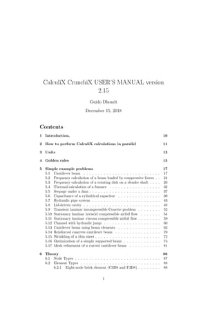
  • 17. 17 8 1 1 F=9MN z x y y m m m Figure 1: Geometry and boundary conditions of the beam problem 6. if you experience a segmentation fault, you may set the environment vari- able CCX LOG ALLOC to 1 by typing “export CCX LOG ALLOC=1” in a terminal window. Running CalculiX you will get information on which fields are allocated, reallocated or freed at which line in the code (default is 0). 7. this is for experts: if you experience problems with dependencies between different equations you can print the SPC’s at the beginning of each step by removing the comment in front of the call to writeboun in ccx 2.15.c and recompile, and you can print the MPC’s each time they are set up by decommenting the loop in which writempc is called at the beginning of cascade.c and recompile. 5 Simple example problems 5.1 Cantilever beam In this section, a cantilever beam loaded by point forces at its free end is ana- lyzed. The geometry, loading and boundary conditions of the cantilever beam are shown in Figure 1. The size of the beam is 1x1x8 m3 , the loading consists of a point force of 9 × 10⁶ N and the beam is completely fixed (in all directions) on the left end. Let us take 1 m and 1 MN as units of length and force, respectively. Assume that the beam geometry was generated and meshed with CalculiX GraphiX (cgx) resulting in the mesh in Figure 2. For reasons of clarity, only element labels are displayed. A CalculiX input deck basically consists of a model definition section de- scribing the geometry and boundary conditions of the problem and one or more steps (Figure 3) defining the loads. The model definition section starts at the beginning of the file and ends at the occurrence of the first *STEP card. All input is preceded by keyword cards, which all start with an asterisk (*), indicating the kind of data which follows. *STEP is such a keyword card. Most keyword cards are either model definition cards (i.e. they can only occur before the first *STEP card) or step cards (i.e.
  • 18. 18 5 SIMPLE EXAMPLE PROBLEMS Figure 2: Mesh for the beam
  • 19. 5.1 Cantilever beam 19 material description *END STEP *STEP *STEP *END STEP *STEP *END STEP Step n Step 2 Step 1 Model Definition Figure 3: Structure of a CalculiX input deck
  • 20. 20 5 SIMPLE EXAMPLE PROBLEMS they can only occur between *STEP and *END STEP cards). A few can be both. In our example (Figure 4), the first keyword card is *HEADING, followed by a short description of the problem. This has no effect on the output and only serves for identification. Then, the coordinates are given as triplets preceded by the *NODE keyword. Notice that data on the same line are separated by commas and must not exceed a record length of 132 columns. A keyword card can be repeated as often as needed. For instance, each node could have been preceded by its own *NODE keyword card. Next, the topology is defined by use of the keyword card *ELEMENT. Defin- ing the topology means listing for each element its type, which nodes belong to the element and in what order. The element type is a parameter on the keyword card. In the beam case 20-node brick elements with reduced integration have been used, abbreviated as C3D20R. In addition, by adding ELSET=Eall, all elements following the *ELEMENT card are stored in set Eall. This set will be later referred to in the material definition. Now, each element is listed followed by the 20 node numbers defining it. With *NODE and *ELEMENT, the core of the geometry description is finished. Remaining model definition items are geometric boundary conditions and the material description. The only geometric boundary condition in the beam problem is the fixation at z=0. To this end, the nodes at z=0 are collected and stored in node set FIX defined by the keyword card *NSET. The nodes belonging to the set follow on the lines underneath the keyword card. By means of the card *BOUNDARY, the nodes belonging to set FIX are subsequently fixed in 1, 2 and 3-direction, corresponding to x,y and z. The three *BOUNDARY statements in Figure 4 can actually be grouped yielding: *BOUNDARY FIX,1 FIX,2 FIX,3 or even shorter: *BOUNDARY FIX,1,3 meaning that degrees of freedom 1 through 3 are to be fixed (i.e. set to zero). The next section in the input deck is the material description. This section is special since the cards describing one and the same material must be grouped together, although the section itself can occur anywhere before the first *STEP card. A material section is always started by a *MATERIAL card defining the name of the material by means of the parameter NAME. Depending on the kind of material several keyword cards can follow. Here, the material is linear elastic, characterized by a Young’s modulus of 210,000.0 MN/m2 and a Poisson coefficient of 0.3 (steel). These properties are stored beneath the
  • 21. 5.1 Cantilever beam 21 *HEADING Model: beam Date: 10−Mar−1998 *NODE 1, 0.000000, 0.000000, 0.000000 2, 1.000000, 0.000000, 0.000000 3, 1.000000, 1.000000, 0.000000 . . . 260, 0.500000, 0.750000, 7.000000 261, 0.500000, 0.500000, 7.500000 *ELEMENT, TYPE=C3D20R , ELSET=Eall 1, 1, 10, 95, 19, 61, 105, 222, 192, 9, 93, 94, 20, 104, 220, 221, 193, 62, 103, 219, 190 2, 10, 2, 13, 95, 105, 34, 134, 222, 11, 12, 96, 93, 106, 133, 223, 220, 103, 33, 132, 219 . . . . 32, 258, 158, 76, 187, 100, 25, 7, 28, 259, 159, 186, 260, 101, 26, 27, 102, 261, 160, 77, 189 *NSET, NSET=FIX 97, 96, 95, 94, 93, 20, 19, 18, 17, 16, 15, 14, 13, 12, 11, 10, 9, 4, 3, 2, 1 *BOUNDARY FIX, 1 *BOUNDARY FIX, 2 *BOUNDARY FIX, 3 *NSET,NSET=Nall,GENERATE 1,261 *MATERIAL,NAME=EL *ELASTIC 210000.0, .3 *SOLID SECTION,ELSET=Eall,MATERIAL=EL *NSET,NSET=LOAD 5,6,7,8,22,25,28,31,100 ** *STEP *STATIC *CLOAD LOAD,2,1. *NODE PRINT,NSET=Nall U *EL PRINT,ELSET=Eall S *NODE FILE U *EL FILE S *END STEP Figure 4: Beam input deck
  • 22. 22 5 SIMPLE EXAMPLE PROBLEMS Figure 5: Deformation of the beam *ELASTIC keyword card, which here concludes the material definition. Next, the material is assigned to the element set Eall by means of the keyword card *SOLID SECTION. Finally, the last card in the model definition section defines a node set LOAD which will be needed to define the load. The card starting with two asterisks in between the model definition section and the first step section is a comment line. A comment line can be introduced at any place. It is completely ignored by CalculiX and serves for input deck clarity only. In the present problem, only one step is needed. A step always starts with a *STEP card and concludes with a *END STEP card. The keyword card *STATIC defines the procedure. The *STATIC card indicates that the load is applied in a quasi-static way, i.e. so slow that mass inertia does not play a role. Other procedures are *FREQUENCY, *BUCKLE, *MODAL DYNAMIC, *STEADY STATE DYNAMICS and *DYNAMIC. Next, the concentrated load is applied (keyword *CLOAD) to node set LOAD. The forces act in y-direction and their magnitude is 1, yielding a total load of 9. Finally, the printing and file storage cards allow for user-directed output generation. The print cards (*NODE PRINT and *EL PRINT) lead to an ASCII file with extension .dat. If they are not selected, no .dat file is generated. The *NODE PRINT and *EL PRINT cards must be followed by the node and element sets for which output is required, respectively. Element information is stored at the integration points. The *NODE FILE and *EL FILE cards, on the other hand, govern the output written to an ASCII file with extension .frd. The results in this file can
  • 23. 5.1 Cantilever beam 23 Figure 6: Axial normal stresses in the beam be viewed with CalculiX GraphiX (cgx). Quantities selected by the *NODE FILE and *EL FILE cards are always stored for the complete model. Element quantities are extrapolated to the nodes, and all contributions in the same node are averaged. Selection of fields for the *NODE PRINT, *EL PRINT, *NODE FILE and *EL FILE cards is made by character codes: for instance, U are the displacements and S are the (Cauchy) stresses. The input deck is concluded with an *END STEP card. The output files for the beam problem consist of file beam.dat and beam.frd. The beam.dat file contains the displacements for set Nall and the stresses in the integration points for set Eall. The file beam.frd contains the displacements and extrapolated stresses in all nodes. It is the input for the visualization program CalculiX GraphiX (cgx). An impression of the capabilities of cgx can be obtained by looking at Figures 5, 6 and 7. Figure 5 shows the deformation of the beam under the prevailing loads. As expected, the beam bends due to the lateral force at its end. Figure 6 shows the normal stress in axial direction. Due to the bending moment one obtains a nearly linear distribution across the height of the beam. Finally, Figure 7 shows the Von Mises stress in the beam.
  • 24. 24 5 SIMPLE EXAMPLE PROBLEMS Figure 7: Von Mises stresses in the beam 5.2 Frequency calculation of a beam loaded by compres- sive forces Let us consider the beam from the previous section and determine its eigenfre- quencies and eigenmodes. To obtain different frequencies for the lateral direc- tions the cross section is changed from 1x1 to 1x1.5. Its length is kept (8 length units). The input deck is very similar to the one in the previous section, Figure 8. The full deck is part of the test example suite (beamf2.inp). The only significant differences relate to the steps. In the first step the preload is applied in the form of compressive forces at the end of the beam. In each node belonging to set LAST a compressive force is applied with a value of -48.155 in the positive z-direction, or, which is equivalent, with magnitude 48.155 in the negative z-direction. The second step is a frequency step. By using the parameter PERTURBATION on the *STEP keyword card the user specifies that the deformation and stress from the previous static step should be taken into account in the subsequent frequency calculation. The *FREQUENCY card and the line underneath indicate that this is a modal analysis step and that the 10 lowest eigenfrequencies are to be determined. They are automatically stored in the .dat file. Table 2 shows these eigenfrequencies for the beam without and with preload together with a comparison with ABAQUS (the input deck for the modal analysis without preload is stored in file beamf.inp of the test example suite). One notices that due to the preload the eigenfrequencies drop. This is especially outspoken for the lower frequencies. As a matter of fact, the lowest
  • 25. 5.2 Frequency calculation of a beam loaded by compressive forces 25 ** ** Structure: beam under compressive forces. ** Test objective: Frequency analysis; the forces are that ** high that the lowest frequency is nearly ** zero, i.e. the buckling load is reached. ** *HEADING Model: beam Date: 10−Mar−1998 *NODE 1, 0.000000, 0.000000, 0.000000 . . *ELEMENT, TYPE=C3D20R 1, 1, 10, 95, 19, 61, 105, 222, 192, 9, 93, 94, 20, 104, 220, 221, 193, 62, 103, 219, 190 . . *NSET, NSET=CN7 97, 96, 95, 94, 93, 20, 19, 18, 17, 16, 15, 14, 13, 12, 11, 10, 9, 4, 3, 2, 1 *BOUNDARY CN7, 1 *BOUNDARY CN7, 2 *BOUNDARY CN7, 3 *ELSET,ELSET=EALL,GENERATE 1,32 *MATERIAL,NAME=EL *ELASTIC 210000.0, .3 *DENSITY 7.8E−9 *SOLID SECTION,MATERIAL=EL,ELSET=EALL *NSET,NSET=LAST 5, 6, . . *STEP *STATIC *CLOAD LAST,3,−48.155 *END STEP *STEP,PERTURBATION *FREQUENCY 10 *NODE FILE U *EL FILE S *END STEP Figure 8: Frequency input deck
  • 26. 26 5 SIMPLE EXAMPLE PROBLEMS Table 2: Frequencies without and with preload (cycles/s). without preload with preload CalculiX ABAQUS CalculiX ABAQUS 13,096. 13,096. 705. 1,780. 19,320. 19,319. 14,614. 14,822. 76,840. 76,834. 69,731. 70,411. 86,955. 86,954. 86,544. 86,870. 105,964. 105,956. 101,291. 102,148. 162,999. 162,998. 162,209. 163,668. 197,645. 197,540. 191,581. 193,065. 256,161. 256,029. 251,858. 253,603. 261,140. 261,086. 259,905. 260,837. 351,862. 351,197. 345,729. 347,688. bending eigenfrequency is so low that buckling will occur. Indeed, one way of determining the buckling load is by increasing the compressive load up to the point that the lowest eigenfrequency is zero. For the present example this means that the buckling load is 21 x 48.155 = 1011.3 force units (the factor 21 stems from the fact that the same load is applied in 21 nodes). An alternative way of determining the buckling load is to use the *BUCKLE keyword card. This is illustrated for the same beam geometry in file beamb.inp of the test suite. Figures 9 and 10 show the deformation of the second bending mode across the minor axis of inertia and deformation of the first torsion mode. 5.3 Frequency calculation of a rotating disk on a slender shaft This is an example for a complex frequency calculation. A disk with an outer diameter of 10, an inner diameter of 2 and a thickness of 0.25 is mounted on a hollow shaft with outer diamter 2 and inner diameter 1 (example rotor.inp in het test examples). The disk is mounted in het middle of the shaft, the ends of which are fixed in all directions. The length of the shaft on either side of the disk is 50. The input deck for this example is shown in Figure 11. The deck start with the definition of the nodes and elements. The set Nfix contains the nodes at the end of the shaft, which are fixed in all directions. The material is ordinary steel. Notice that the density is needed for the centrifugal loading. Since the disk is rotation there is a preload in the form of centrifugal forces. Therefore, the first step is a nonlinear geometric static step in order to calculate the deformation and stresses due to this loading. By selecting the parameter perturbation in the subsequent frequency step this preload is taken into account in the calculation of the stiffness matrix in the frequency calculation. The
  • 27. 5.3 Frequency calculation of a rotating disk on a slender shaft 27 Figure 9: Second bending mode across the minor axis of inertia Figure 10: First torsion mode
  • 28. 28 5 SIMPLE EXAMPLE PROBLEMS Figure 11: Input deck for the rotor
  • 29. 5.3 Frequency calculation of a rotating disk on a slender shaft 29 Figure 12: Eigenfrequencies for the rotor
  • 30. 30 5 SIMPLE EXAMPLE PROBLEMS Figure 13: Eigenfrequencies as a function of shaft speed resulting eigenfrequencies are stored at the top of file rotor.dat (Figure 12 for a rotational speed of 9000 rad/s). In a *FREQUENCY step an eigenvalue problem is solved, the eigenvalues of which (first column on the top of Figure 12) are the square of the eigenfrequencies of the structure (second to fourth column). If the eigenvalue is negative, an imaginary eigenfrequency results. This is the case for the two lowest eigenvalues for the rotor rotating at 9000 rad/s. For shaft speeds underneath about 6000 rad/s all eigenfrequencies are real. The lowest eigenfrequencies as a function of rotating speeds up to 18000 rad/s are shown in Figure 13 (+ and x curves). What is the physical meaning of imaginary eigenfrequencies? The eigen- modes resulting from a frequency calculation contain the term eiωt . If the eigenfrequency ω is real, one obtains a sine or cosine, if ω is imaginary, one ob- tains an increasing or decreasing exponential function [18]. Thus, for imaginary eigenfrequencies the response is not any more oscillatory: it increases indefi- nitely, the system breaks apart. Looking at Figure 13 one observes that the lowest eigenfrequency decreases for increasing shaft speed up to the point where it is about zero at a shaft speed of nearly 6000 rad/s. At that point the eigenfre- quency becomes imaginary, the rotor breaks apart. This has puzzled engineers for a long time, since real systems were observed to reach supercritical speeds without breaking apart. The essential point here is to observe that the calculations are being per- formed in a rotating coordinate system (fixed to the shaft). Newton’s laws are not valid in an accelerating reference system, and a rotating coordinate system
  • 31. 5.3 Frequency calculation of a rotating disk on a slender shaft 31 Figure 14: Two-node eigenmode is accelerating. A correction term to Newton’s laws is necessary in the form of a Coriolis force. The introduction of the Coriolis force leads to a complex nonlin- ear eigenvalue system, which can solved with the *COMPLEX FREQUENCY procedure (cf. Section 6.9.3). One can prove that the resulting eigenfrequencies are real, the eigenmodes, however, are usually complex. This leads to rotating eigenmodes. In order to use the *COMPLEX FREQUENCY procedure the eigenmodes without Coriolis force must have been calculated and stored in a previous *FRE- QUENCY step (STORAGE=YES) (cf. Figure 11). The complex frequency re- sponse is calculated as a linear combination of these eigenmodes. The number of eigenfrequencies requested in the *COMPLEX FREQUENCY step should not exceed those of the preceding *FREQUENCY step. Since the eigenmodes are complex, they are best stored in terms of amplitude and phase with PU underneath the *NODE FILE card. The correct eigenvalues for the rotating shaft lead to the straight lines in Figure 13. Each line represents an eigenmode: the lowest decreasing line is a two-node counter clockwise (ccw) eigenmode when looking in (-z)-direction, the highest decreasing line is a three-node ccw eigenmode, the lowest and highest increasing lines constitute both a two-node clockwise (cw) eigenmode. A node is a location at which the radial motion is zero. Figure 14 shows the two-node eigenmode, Figure 15 the three-node eigenmode. Notice that if the scales on the x- and y-axis in Figure 13 were the same the lines would be under 45◦ . It might surprise that both increasing straight lines correspond to one and the same eigenmode. For instance, for a shaft speed of 5816 rad/s one and the same eigenmode occurs at an eigenfrequency of 0 and 11632 rad/s. Remember, however, that the eigenmodes are calculated in the rotating system, i.e. as
  • 32. 32 5 SIMPLE EXAMPLE PROBLEMS Figure 15: Three-node eigenmode observed by an observer rotating with the shaft. To obtain the frequencies for a fixed observer the frequencies have to be considered relative to a 45◦ straight line through the origin and bisecting the diagram. This observer will see one and the same eigenmode at 5816 rad/s and -5816 rad/s, so cw and ccw. Finally, the Coriolis effect is not always relevant. Generally, slender rotat- ing structures (large blades...) will exhibit important frequency shifts due to Coriolis. 5.4 Thermal calculation of a furnace This problem involves a thermal calculation of the furnace depicted in Figure 16. The furnace consists of a bottom plate at a temperature T b, which is prescribed. It changes linearly in an extremely short time from 300 K to 1000 K after which it remains constant. The side walls of the furnace are isolated from the outer world, but exchange heat through radiation with the other walls of the furnace. The emissivity of the side walls and bottom is ǫ = 1. The top of the furnace exchanges heat through radiation with the other walls and with the environmental temperature which is fixed at 300 K. The emissivity of the top is ǫ = 0.8. Furthermore, the top exchanges heat through convection with a fluid (air) moving at the constant rate of 0.001 kg/s. The temperature of the fluid at the right upper corner is 300 K. The walls of the oven are made of 10 cm steel. The material constants for steels are: heat conductivity κ = 50W/mK, specific heat c = 446W/kgK and density ρ = 7800kg/m3 . The material constants for air are : specific heat cp = 1000W/kgK and density ρ = 1kg/m3 . The convection coefficient is h = 25W/m2 K. The dimensions of the furnace are 0.3 × 0.3 × 0.3m3 (cube). At t = 0 all parts are at T = 300K. We would like to
  • 33. 5.4 Thermal calculation of a furnace 33 T=300 K T=300 K T b ε=1 ε=1 ε=1 isolated isolated ε=0.8 1000 1 0 300 t(s) Tb(K) ε=0.8 A B h=25 W/mK D E C x z 0.3 m dm/dt = 0.001 kg/s Figure 16: Description of the furnace know the temperature at locations A,B,C,D and E as a function of time. The input deck is listed in Figure 17. It starts with the node definitions. The highest node number in the structure is 602. The nodes 603 up to 608 are fluid nodes, i.e. in the fluid extra nodes were defined (z=0.3 corresponds with the top of the furnace, z=0 with the bottom). Fluid node 603 corresponds to the location where the fluid temperature is 300 K (“inlet”), node 608 corresponds to the “outlet”, the other nodes are located in between. The coordinates of the fluid nodes actually do not enter the calculations. Only the convective defini- tions with the keyword *FILM govern the exchange between furnace and fluid. With the *ELEMENT card the 6-node shell elements making up the furnace walls are defined. Furthermore, the fluid nodes are also assigned to elements (element type D), so-called network elements. These elements are needed for the assignment of material properties to the fluid. Indeed, traditionally material properties are assigned to elements and not to nodes. Each network element consists of two end nodes, in which the temperature is unknown, and a midside node, which is used to define the mass flow rate through the element. The fluid nodes 603 up to 613 are assigned to the network elements 301 up to 305. Next, two node sets are defined: GAS contains all fluid nodes, Ndown con- tains all nodes on the bottom of the furnace. The *PHYSICAL CONSTANTS card is needed in those analyses in which radiation plays a role. It defines absolute zero, here 0 since we work in Kelvin, and the Stefan Boltzmann constant. In the present input deck SI units are used
  • 34. 34 5 SIMPLE EXAMPLE PROBLEMS furnace.txt Sun Feb 12 13:12:10 2006 1 *NODE, NSET=Nall 1, 3.00000e−01, 3.72529e−09, 3.72529e−09 ... 603,−0.1,0.5,1. ... 613,0.8,0.5,1. *ELEMENT, TYPE=S6, ELSET=furnace 1, 1, 2, 3, 4, 5, 6 ... *ELEMENT,TYPE=D,ELSET=EGAS 301,603,609,604 ... 305,607,613,608 *NSET,NSET=NGAS,GENERATE 603,608 *NSET,NSET=Ndown 1, ... *PHYSICAL CONSTANTS,ABSOLUTE ZERO=0.,STEFAN BOLTZMANN=5.669E−8 *MATERIAL,NAME=STEEL *DENSITY 7800. *CONDUCTIVITY 50. *SPECIFIC HEAT 446. *SHELL SECTION,ELSET=furnace,MATERIAL=STEEL 0.01 *MATERIAL,NAME=GAS *DENSITY 1. *SPECIFIC HEAT 1000. *FLUID SECTION,ELSET=EGAS,MATERIAL=GAS *INITIAL CONDITIONS,TYPE=TEMPERATURE Nall,300. *AMPLITUDE,NAME=A1 0.,.3,1.,1. *STEP,INC=100 *HEAT TRANSFER 0.1,1. *BOUNDARY,AMPLITUDE=A1 Ndown,11,11,1000. *BOUNDARY 603,11,11,300. *BOUNDARY 609,1,1,0.001 ... *RADIATE ** Radiate based on down 1, R1CR,1000., 1.000000e+00 ... ** Radiate based on top 51, R1CR, 1000.000000, 8.000000e−01 ... ** Radiate based on side 101, R1CR, 1000.000000, 1. ... ** Radiate based on top 51, R2, 300.000000, 8.000000e−01 ... *FILM 51, F2FC, 604, 2.500000e+01 ... *NODE FILE NT *NODE PRINT,NSET=NGAS NT *END STEP Figure 17: Input deck for the furnace
  • 35. 5.4 Thermal calculation of a furnace 35 throughout. Next, the material constants for STEEL are defined. For thermal analyses the conductivity, specific heat and density must be defined. The *SHELL SEC- TION card assigns the STEEL material to the element set FURNACE, defined by the *ELEMENT statement before. It contains all elements belonging to the furnace. Furthermore, a thickness of 0.01 m is assigned. The material constants for material GAS consist of the density and the specific heat. These are the constants for the fluid. Conduction in the fluid is not considered. The material GAS is assigned to element set EGAS containing all network elements. The *INITIAL CONDITIONS card defines an initial temperature of 300 K for all nodes, i.e. furnace nodes AND fluid nodes. The *AMPLITUDE card defines a ramp function starting at 0.3 at 0.0 and increasing linearly to 1.0 at 1.0. It will be used to define the temperature boundary conditions at the bottom of the furnace. This ends the model definition. The first step describes the linear increase of the temperature boundary con- dition between t = 0 and t = 1. The INC=100 parameter on the *STEP card allows for 100 increments in this step. The procedure is *HEAT TRANSFER, i.e. we would like to perform a purely thermal analysis: the only unknowns are the temperature and there are no mechanical unknowns (e.g. displace- ments). The step time is 1., the initial increment size is 0.1. Both appear on the line underneath the *HEAT TRANSFER card. The absence of the param- eter STEADY STATE on the *HEAT TRANSFER card indicates that this is a transient analysis. Next come the temperature boundary conditions: the bottom plate of the furnace is kept at 1000 K, but is modulated by amplitude A1. The result is that the temperature boundary condition starts at 0.3 x 1000 = 300K and increases linearly to reach 1000 K at t=1 s. The second boundary conditions specifies that the temperature of (fluid) node 603 is kept at 300 K. This is the inlet temperature. Notice that “11” is the temperature degree of freedom. The mass flow rate in the fluid is defined with the *BOUNDARY card applied to the first degree of freedom of the midside nodes of the network elements. The first line tells us that the mass flow rate in (fluid)node 609 is 0.001. Node 609 is the midside node of network element 301. Since this rate is positive the fluid flows from node 603 towards node 604, i.e. from the first node of network element 301 to the third node. The user must assure conservation of mass (this is actually also checked by the program). The first set of radiation boundary conditions specifies that the top face of the bottom of the furnace radiates through cavity radiation with an emissivity of 1 and an environment temperature of 1000 K. For cavity radiation the envi- ronment temperature is used in case the viewfactor at some location does not amount to 1. What is short of 1 radiates towards the environment. The first number in each line is the element, the number in the label (the second entry in each line) is the face of the element exposed to radiation. In general, these lines are generated automatically in cgx (CalculiX GraphiX). The second and third block define the internal cavity radiation in the furnace
  • 36. 36 5 SIMPLE EXAMPLE PROBLEMS Figure 18: Temperature distribution at t=3001 s 200 300 400 500 600 700 800 900 1000 0 500 1000 1500 2000 2500 3000 3500 T (K) Time(s) A B C D E Figure 19: Temperature at selected positions
  • 37. 5.5 Seepage under a dam 37 for the top and the sides. The fourth block defines the radiation of the top face of the top plate of the furnace towards the environment, which is kept at 300 K. The emissivity of the top plate is 0.8. Next come the film conditions. Forced convection is defined for the top face of the top plate of the furnace with a convection coefficient h = 25W/mK. The first line underneath the *FILM keyword indicates that the second face of element 51 interacts through forced convection with (fluid)node 604. The last entry in this line is the convection coefficient. So for each face interacting with the fluid an appropriate fluid node must be specified with which the interaction takes place. Finally, the *NODE FILE card makes sure that the temperature is stored in the .frd file and the *NODE PRINT card takes care that the fluid temperature is stored in the .dat file. The complete input deck is part of the test examples of CalculiX (fur- nace.inp). For the present analysis a second step was appended keeping the bottom temperature constant for an additional 3000 seconds. What happens during the calculation? The walls and top of the furnace heat up due to conduction in the walls and radiation from the bottom. However, the top of the furnace also loses heat through radiation with the environment and convection with the fluid. Due to the interaction with the fluid the temperature is asymmetric: at the inlet the fluid is cool and the furnace will lose more heat than at the outlet, where the temperature of the fluid is higher and the temperature difference with the furnace is smaller. So due to convection we expect a temperature increase from inlet to outlet. Due to conduction we expect a temperature minimum in the middle of the top. Both effects are superimposed. The temperature distribution at t = 3001s is shown in Figure 18. There is a temperature gradient from the bottom of the furnace towards the top. At the top the temperature is indeed not symmetric. This is also shown in Figure 19, where the temperature of locations A, B, C, D and E is plotted as a function of time. Notice that steady state conditions have not been reached yet. Also note that 2D elements (such as shell elements) are automatically expanded into 3D elements with the right thickness. Therefore, the pictures, which were plotted from within CalculiX GraphiX, show 3D elements. 5.5 Seepage under a dam In this section, groundwater flow under a dam is analyzed. The geometry of the dam is depicted in Figure 20 and is taken from exercise 30 in Chapter 1 of [27]. All length measurements are in feet (0.3048 m). The water level upstream of the dam is 20 feet high, on the downstream side it is 5 feet high. The soil underneath the dam is anisotropic. Upstream the permeability is characterized by k1 = 4k2 = 10−2 cm/s, downstream we have 25k3 = 100k4 = 10−2 cm/s. Our primary interest is the hydraulic gradient, i.e. ∇h since this is a measure whether or not piping will occur. Piping means that the soil is being carried away by the groundwater flow (usually at the downstream side) and constitutes
  • 38. 38 5 SIMPLE EXAMPLE PROBLEMS an instable condition. As a rule of thumb, piping will occur if the hydraulic gradient is about unity. From Section 6.9.14 we know that the equations governing stationary ground- water flow are the same as the heat equations. The equivalent quantity of the total head is the temperature and of the velocity it is the heat flow. For the finite element analysis SI units were taken, so feet was converted into meter. Furthermore, a vertical impermeable wall was assumed far upstream and far downstream (actually, 30 m upstream from the middle point of the dam and 30 m downstream). Now, the boundary conditions are: 1. the dam, the left and right vertical boundaries upstream and downstream, and the horizontal limit at the bottom are impermeable. This means that the water velocity perpendicular to these boundaries is zero, or, equiva- lently, the heat flux. 2. taking the reference for the z-coordinate in the definition of total head at the bottom of the dam (see Equation 330 for the definition of total head), and assuming that the atmospheric pressure p0 is zero, the total head upstream is 28 feet and downstream it is 13 feet. In the thermal equivalent this corresponds to temperature boundary conditions. The input deck is summarized in Figure 21. The complete deck is part of the example problems. The problem is really two-dimensional and consequently qu8 elements were used for the mesh generation within CalculiX GraphiX. To obtain a higher resolution immediately adjacent to the dam a bias was used (the mesh can be seen in Figure 22). At the start of the deck the nodes are defined and the topology of the el- ements. The qu8 element type in CalculiX GraphiX is by default translated by the send command into a S8 (shell) element in CalculiX CrunchiX. How- ever, a plane element is here more appropriate. Since the calculation at stake is thermal and not mechanical, it is really immaterial whether one takes plane strain (CPE8) or plane stress (CPS8) elements. With the *ELSET keyword the element sets for the two different kinds of soil are defined. The nodes on which the constant total head is to be applied are defined by *NSET cards. The permeability of the soil corresponds to the heat conduction coefficient in a thermal analysis. Notice that the permeability is defined to be orthotropic, using the *CONDUCTIVITY,TYPE=ORTHO card. The values beneath this card are the permeability in x, y and z-direction (SI units: m/s). The value for the z-direction is actually immaterial, since no gradient is expected in that direction. The *SOLID SECTION card is used to assign the materials to the ap- propriate soil regions. The *INITIAL CONDITIONS card is not really needed, since the calculation is stationary, however, CalculiX CrunchiX formally needs it in a heat transfer calculation. Within the step a *HEAT TRANSFER, STEADY STATE calculation is selected without any additional time step information. This means that the defaults for the step length (1) and initial increment size (1) will be taken. With
  • 39. 5.6 Capacitance of a cylindrical capacitor 39 20’ 60’ 8’ 20’ 5’ 20’ 2 1 4 3 area1 area2 Figure 20: Geometry of the dam the *BOUNDARY cards the total head upstream and downstream is defined (11 is the temperature degree of freedom). Finally, the *NODE PRINT, *NODE FILE and *EL FILE cards are used to define the output: NT is the temperature, or, equivalently, the total head (Figure 22) , and HFL is the heat flux, or, equivalently, the groundwater flow velocity (y-component in Figure 23). Since the permeability upstream is high, the total head gradient is small. The converse is true downstream. The flow velocity is especially important downstream. There it reaches values up to 2.25 × 10⁻⁴ m/s (the red spot in Figure 23), which corresponds to a hydraulic gradient of about 0.56, since the permeability in y-direction downstream is 4×10⁻⁴ m/s. This is smaller than 1, so no piping will occur. Notice that the velocity is naturally highest immediately next to the dam. This example shows how seepage problems can be solved by using the heat transfer capabilities in CalculiX GraphiX. The same applies to any other phe- nomenon governed by a Laplace-type equation. 5.6 Capacitance of a cylindrical capacitor In this section the capacitance of a cylindrical capacitor is calculated with inner radius 1 m, outer radius 2 m and length 10 m. The capacitor is filled with air, its permittivity is ǫ0 = 8.8542 × 10⁻¹² C2 /Nm2 . An extract of the input deck, which is part of the test example suite, is shown below: *NODE, NSET=Nall ... *ELEMENT, TYPE=C3D20, ELSET=Eall
  • 40. 40 5 SIMPLE EXAMPLE PROBLEMS dam.txt Sun Feb 12 13:17:58 2006 1 ** ** Structure: dam. ** Test objective: groundwater flow analysis. ** *NODE, NSET=Nall 1, −3.00000e+01, −1.34110e−07, 0.00000e+00 2, −3.00000e+01, −4.53062e−01, 0.00000e+00 3, −2.45219e+01, −4.53062e−01, 0.00000e+00 ... *ELEMENT, TYPE=CPS8, ELSET=Eall 1, 1, 2, 3, 4, 5, 6, 7, 8 2, 4, 3, 9, 10, 7, 11, 12, 13 3, 10, 9, 14, 15, 12, 16, 17, 18 ... *ELSET,ELSET=Earea1 1, 2, ... *ELSET,ELSET=Earea2 161, 162, ... *NSET,NSET=Nup 342, 345, ... *NSET,NSET=Ndown 982, 985, ... *MATERIAL,NAME=MAT1 *CONDUCTIVITY,TYPE=ORTHO 1.E−2,25.E−4,1.E−4 *MATERIAL,NAME=MAT2 *CONDUCTIVITY,TYPE=ORTHO 1.E−4,4.E−4,1.E−4 *SOLID SECTION,ELSET=Earea1,MATERIAL=MAT1 *SOLID SECTION,ELSET=Earea2,MATERIAL=MAT2 *INITIAL CONDITIONS,TYPE=TEMPERATURE Nall,0. ** *STEP *HEAT TRANSFER,STEADY STATE *BOUNDARY Nup,11,11,8.5344 *BOUNDARY Ndown,11,11,3.9624 *NODE PRINT,NSET=Nall NT *NODE FILE NT *EL FILE HFL *END STEP Figure 21: Input deck of the dam problem
  • 41. 5.6 Capacitance of a cylindrical capacitor 41 Figure 22: Total head Figure 23: Discharge velocity in y-direction
  • 42. 42 5 SIMPLE EXAMPLE PROBLEMS Figure 24: Heat flux in the capacitor’s thermal analogy ... *NSET,NSET=Nin 1, 2, ... *NSET,NSET=Nout 57, 58, ... *SURFACE,NAME=S1,TYPE=ELEMENT 6,S3 1,S3 *MATERIAL,NAME=EL *CONDUCTIVITY 8.8541878176e-12 *SOLID SECTION,ELSET=Eall,MATERIAL=EL *STEP *HEAT TRANSFER,STEADY STATE *BOUNDARY Nin,11,11,2. Nout,11,11,1. *EL FILE HFL
  • 43. 5.7 Hydraulic pipe system 43 *SECTION PRINT,SURFACE=S1 FLUX *END STEP As explained in Section 6.9.13 the capacitance can be calculated by deter- mining the total heat flux through one of the capacitor’s surfaces due to a unit temperature difference between the surfaces. The material in between the sur- faces of the capacitor is assigned a conductivity equal to its permittivity. Here, only one degree of the capacitor has been modeled. In axial direction the mesh is very coarse, since no variation of the temperature is expected. Figure 24 shows that the heat flux at the inner radius is 1.27 × 10⁻¹¹ W/m2 . This corresponds to a total heat flow of 7.98−10 W. The analytical formula for the capacitor yields 2πǫ0/ ln(2) = 8.0261−10 C/V. The total flux through the inner surface S1 is also stored in the .dat file because of the *SECTION PRINT keyword card in the input deck. It amounts to −2.217 × 10⁻¹² W. This value is negative, because the flux is entering the space in between the capacitor’s surfaces. Since only one degree was modeled, this value has to be multiplied by 360 and yields the same value as above. 5.7 Hydraulic pipe system In CalculiX it is possible to perform steady-state hydraulic and aerodynamic network calculations, either as stand-alone applications, or together with me- chanical and/or thermal calculations of the adjacent structures. Here, a stand- alone hydraulic network discussed in [10] is analyzed. The input deck pipe.f can be found in the test suite. The geometry of the network is shown in Figure 25. It is a linear network consisting of: • an upstream reservoir with surface level at 14.5 m • an entrance with a contraction of 0.8 • a pipe with a length of 5 m and a diameter of 0.2 m • a bend of 45 o and a radius of 0.3 m • a pipe with a length of 5 m and a diameter of 0.2 m • a pipe with a length of 5 m and a diameter of 0.3 m • a pipe with a length of 2.5 m and a diameter of 0.15 m • a gate valve in E with α = 0.5 • a pipe with a length of 1.56 m and a diameter of 0.15 m • an exit in a reservoir with surface level at 6.5 m
  • 44. 44 5 SIMPLE EXAMPLE PROBLEMS 5.00 5.00 5.00 2.50 A B C D E F B: Bend R=0.3 m AB: Pipe D=0.2 m, Manning n=0.015 BC: Pipe D=0.2 m, Manning n=0.015 DE: Pipe D=0.15 m, Manning n=0.015 EF: Pipe D=0.15 m, Manning n=0.015 45° 1.56 A: A0/A=0.8 E: Gate Valve, alpha=0.5 14.50 10.15 0.00 6.50 CD: Pipe D=0.3 m, Manning n=0.015 Figure 25: Geometry of the hydraulic network All pipes are characterized by a Manning friction coefficient n=0.015. The input deck looks like: ** ** Structure: pipe connecting two reservoirs. ** Test objective: hydraulic network. ** *NODE,NSET=NALL 2,0.,0.,14.5 3,0.,0.,14.5 4,0.,0.,12.325 ... 26,14.9419,0.,6.5 *ELEMENT,TYPE=D,ELSET=EALL 1,0,2,3 2,3,4,5 ... 13,25,26,0 *MATERIAL,NAME=WATER *DENSITY 1000. *FLUID CONSTANTS 4217.,1750.E-6,273.
  • 45. 5.7 Hydraulic pipe system 45 *ELSET,ELSET=E1 2 *ELSET,ELSET=E2 3,5 *ELSET,ELSET=E3 4 *ELSET,ELSET=E4 6 *ELSET,ELSET=E5 7 *ELSET,ELSET=E6 8 *ELSET,ELSET=E7 9,11 *ELSET,ELSET=E8 10 *ELSET,ELSET=E9 12 *ELSET,ELSET=E10 1,13 *FLUID SECTION,ELSET=E1,TYPE=PIPE ENTRANCE,MATERIAL=WATER 0.031416,0.025133 *FLUID SECTION,ELSET=E2,TYPE=PIPE MANNING,MATERIAL=WATER 0.031416,0.05,0.015 *FLUID SECTION,ELSET=E3,TYPE=PIPE BEND,MATERIAL=WATER 0.031416,1.5,45.,0.4 *FLUID SECTION,ELSET=E4,TYPE=PIPE ENLARGEMENT,MATERIAL=WATER 0.031416,0.070686 *FLUID SECTION,ELSET=E5,TYPE=PIPE MANNING,MATERIAL=WATER 0.070686,0.075,0.015 *FLUID SECTION,ELSET=E6,TYPE=PIPE CONTRACTION,MATERIAL=WATER 0.070686,0.017671 *FLUID SECTION,ELSET=E7,TYPE=PIPE MANNING,MATERIAL=WATER 0.017671,0.0375,0.015 *FLUID SECTION,ELSET=E8,TYPE=PIPE GATE VALVE,MATERIAL=WATER 0.017671,0.5 *FLUID SECTION,ELSET=E9,TYPE=PIPE ENLARGEMENT,MATERIAL=WATER 0.017671,1.E6 *FLUID SECTION,ELSET=E10,TYPE=PIPE INOUT,MATERIAL=WATER *BOUNDARY 3,2,2,1.E5 25,2,2,1.E5 *STEP *HEAT TRANSFER,STEADY STATE *DLOAD EALL,GRAV,9.81,0.,0.,-1.
  • 46. 46 5 SIMPLE EXAMPLE PROBLEMS *NODE PRINT,NSET=NALL U *END STEP In CalculiX linear networks are modeled by means of 3-node network ele- ments (D-type elements). In the corner nodes of the element the temperature and the pressure are unknown. They are assigned to the degrees of freedom 0 and 2, respectively. In the midside node the mass flux is unknown and is assigned to degree of freedom 1. The properties of the network elements are defined by the keyword *FLUID SECTION. They are treated extensively in Section 6.4 (gases), 6.5 (liquid pipes) and 6.6 (liquid channels). For the network at stake we need: • a dummy network entrance element expressing that liquid is entering the network (element 1). It is characterized by a node number 0 as first node • a network element of type PIPE ENTRANCE at location A (element 2). This element also takes the water depth into account. Notice that there is no special reservoir element. Differences in water level can be taken into account in any element type by assigning the appropriate coordinates to the corner nodes of the element. • a network element of type PIPE MANNING for the pipe between location A and B (element 3) • a network element of type PIPE BEND for the bend at location B (element 4) • a network element of type PIPE MANNING for the pipe between location B and C (element 5) • a network element of type PIPE ENLARGEMENT for the increase of diameter at location C (element 6) • a network element of type PIPE MANNING for the pipe between location C and D (element 7) • a network element of type PIPE CONTRACTION to model the decrease in diameter at location D (element 8) • a network element of type PIPE MANNING for the pipe between location D and E (element 9) • a network element of type PIPE GATE VALVE for the valve at location E (element 10) • a network element of type PIPE MANNING for the pipe between location E and F (element 11)
  • 47. 5.7 Hydraulic pipe system 47 • a network element of type PIPE ENLARGEMENT for the exit in the reservoir (element 12). Indeed, there is no special reservoir entrance ele- ment. A reservoir entrance has to be modeled by a large diameter increase. • a dummy network exit element expressing that liquid is leaving the net- work (element 13) In the input deck, all these elements are defined as D-type elements, their nodes have the correct coordinates and by means of *FLUID SECTION cards each element is properly described. Notice that the dummy network entrance and exit elements are characterized by typeless *FLUID SECTION cards. For a hydraulic network the material properties reduce to the density (on the *DENSITY card), the specific heat and the dynamic viscosity (both on the *FLUID SECTION card). The specific heat is only needed if heat transfer is being modeled. Here, this is not the case. The dynamic viscosity of water is 1750 × 10−6 N s/m2 [34]. The boundary conditions reduce to the atmospheric pressure in node 3 and 25, both at the liquid surface of the reservoir. Remember that the pressure has the degree of freedom 2 in the corner nodes of the network elements. Networks are only active in *COUPLED TEMPERATURE-DISPLACEMENT or *HEAT TRANSFER procedures. Here, we do not take the structure into ac- count, so a heat transfer analysis will do. Finally, the gravity loading has to be specified, this is indeed essential for hydraulic networks. Regarding the nodal output, remember that NT requests degree of freedom 0, whereas U requests degrees of freedom 1 to 3. Since we are interested in the mass flux (DOF 1 in the middle nodes) and the pressure (DOF 2 in the corner nodes), U is selected underneath the *NODE PRINT line. Officially, U are displacements, and that’s the way they are labeled in the .dat file. The results in the .dat file look as follows: displacements (vx,vy,vz) for set NALL and time 1. 2 8.9592E+01 0.0000E+00 0.0000E+00 3 0.0000E+00 1.0000E+05 0.0000E+00 4 8.9592E+01 0.0000E+00 0.0000E+00 5 0.0000E+00 1.3386E+05 0.0000E+00 6 8.9592E+01 0.0000E+00 0.0000E+00 7 0.0000E+00 1.2900E+05 0.0000E+00 8 8.9592E+01 0.0000E+00 0.0000E+00 9 0.0000E+00 1.2859E+05 0.0000E+00 10 8.9592E+01 0.0000E+00 0.0000E+00 11 0.0000E+00 1.5841E+05 0.0000E+00 12 8.9592E+01 0.0000E+00 0.0000E+00 13 0.0000E+00 1.6040E+05 0.0000E+00 14 8.9592E+01 0.0000E+00 0.0000E+00 15 0.0000E+00 1.9453E+05 0.0000E+00
  • 48. 48 5 SIMPLE EXAMPLE PROBLEMS 16 8.9592E+01 0.0000E+00 0.0000E+00 17 0.0000E+00 1.7755E+05 0.0000E+00 18 8.9592E+01 0.0000E+00 0.0000E+00 19 0.0000E+00 1.8361E+05 0.0000E+00 20 8.9592E+01 0.0000E+00 0.0000E+00 21 0.0000E+00 1.5794E+05 0.0000E+00 22 8.9592E+01 0.0000E+00 0.0000E+00 23 0.0000E+00 1.6172E+05 0.0000E+00 24 8.9592E+01 0.0000E+00 0.0000E+00 25 0.0000E+00 1.0000E+05 0.0000E+00 26 8.9592E+01 0.0000E+00 0.0000E+00 The mass flux in the pipe (first DOF in the midside nodes, column 1) is constant and takes the value 89.592 kg/s. This agrees well with the result in [10] of 89.4 l/s. Since not all node and element definitions are listed it is useful for the interpretation of the output to know that location A corresponds to node 5, location B to nodes 7-9, location C to nodes 11-13, location D to nodes 15-17, location E to nodes 19-21 and location F to node 23. The second column in the result file is the pressure. It shows that the bend, the valve and the contraction lead to a pressure decrease, whereas the enlargement leads to a pressure increase (the velocity drops). If the structural side of the network (e.g. pipe walls) is modeled too, the fluid pressure can be mapped automatically onto the structural element faces. This is done by labels of type PxNP in the *DLOAD card. 5.8 Lid-driven cavity The lid-driven cavity is a well-known benchmark problem for viscous incom- pressible fluid flow [85]. The geometry at stake is shown in Figure 26. We are dealing with a square cavity consisting of three rigid walls with no-slip condi- tions and a lid moving with a tangential unit velocity. We are interested in the velocity and pressure distribution for a Reynolds number of 400. The input deck looks like (this deck is also available in the cfd test suite as file lid400.inp): ** ** Structure: lid-driven cavity ** Test objective: incompressible, viscous, laminar, 3D fluid ** *NODE, NSET=Nall 1,5.000000000000e-01,5.000000000000e-01,0.0 ... *ELEMENT, TYPE=F3D8, ELSET=Eall 1, 1, 2, 3, 4, 5, 6, 7, 8 ...
  • 49. 5.8 Lid-driven cavity 49 lid p = 0 no slip walls v=1 1 1 Figure 26: Geometry of the lid-driven cavity
  • 50. 50 5 SIMPLE EXAMPLE PROBLEMS Figure 27: Mesh of the lid-driven cavity *SURFACE, NAME=SOLIDSURFACE 40, S2 ... *MATERIAL,NAME=WATER *DENSITY 1. *FLUID CONSTANTS 1.,.25E-2,293. *SOLID SECTION,ELSET=Eall,MATERIAL=WATER *INITIAL CONDITIONS,TYPE=FLUID VELOCITY Nall,1,0. Nall,2,0. Nall,3,0. *INITIAL CONDITIONS,TYPE=PRESSURE Nall,1. ** *STEP,INCF=5000 *STATIC *BOUNDARYF ** BOUNDARYF based on fixz 1, S3, 3,, 0.000000 ... ** BOUNDARYF based on in
  • 51. 5.8 Lid-driven cavity 51 1601, S1, 1,, 0.000000 ... ** BOUNDARYF based on in 1601, S1, 2,, 1.000000 ... ** BOUNDARYF based on in 1601, S1, 3,, 0.000000 ... ** BOUNDARYF based on wall 40, S2, 1,, 0.000000 ... ** BOUNDARYF based on wall 40, S2, 2,, 0.000000 ... ** BOUNDARYF based on wall 40, S2, 3,, 0.000000 ... *BOUNDARYF 1600, S3, 8,8, 1.000000 *NODE FILE,FREQUENCYF=5000 VF,PSF *END STEP Although the problem is essentially 2-dimensional it was modeled as a 3- dimensional problem with unit thickness since 2-dimensional fluid capabilities are not available in CalculiX. The mesh (2D projection) is shown in Figure 27. It consists of 8-node brick elements. There is one element layer across the thickness. This is sufficient, since the results do not vary in thickness direction. The input deck starts with the coordinates of the nodes and the topology of the elements. The element type for fluid volumetric elements is the same as for structural elements with the C replaced by F (fluid): F3D6. The faces belonging to solid surfaces are listed next. A face is characterized by an element number and an internal face number. Solid surfaces are surfaces at which the fluid adheres, i.e. in the presence of viscosity the velocity vector adjacent to a solid surface is the same as the velocity of the surface itself. All solid surfaces must be collected into a SURFACE definition with the name SOLIDSURFACE (no upper case required, though). The material definition consists of the density, the heat capacity and the dynamic viscosity. The density is set to 1. The heat capacity and the dynamic viscosity are entered underneath the *FLUID CONSTANTS keyword. The heat capacity is not needed since the calculation is steady state, so its value here is irrelevant. The value of the dynamic viscosity was chosen such that the Reynolds number is 400. The Reynolds number is defined as velocity times length divided by the kinematic viscosity. The velocity of the lid is 1, its length is 1 and since the density is 1 the kinematic and dynamic viscosity coincide. Consequently, the kinematic viscosity takes the value 1/400. The material is assigned to the
  • 52. 52 5 SIMPLE EXAMPLE PROBLEMS elements by means of the *SOLID SECTION card. The unknowns of the problem are the velocity and static pressure. No ther- mal boundary conditions are provided, so the temperature is irrelevant. All ini- tial values for the velocity and pressure are set by means of the *INITIAL CON- DITIONS,TYPE=FLUID VELOCITY and *INITIAL CONDITIONS,TYPE=PRESSURE cards. Notice that for the velocity the initial conditions have to be specified for each degree of freedom separately. The step is as usual started with the *STEP keyword. The maximum num- ber of increments, however, is for fluid calculations governed by the parameter INCF. For steady state calculations the keyword *STATIC is to be used. If there are no time increment values beneath this line the increment size is auto- matically chosen such that the procedure is stable. The boundary conditions for fluid calculations are defined on the faces and are prescribed using the *BOUND- ARYF card. Recall that non-homogeneous (i.e. nonzero) boundary conditions have to be defined within a step, homogeneous ones may be defined before or within the step. Here, all boundary conditions have been defined within the step. They include zero velocity at the fixed walls, a velocity of 1 in the y- direction on the lid, and zero velocity in z-direction on the side walls. The pressure has been set to 1 on face 3 of element 1600. In CFD pressure boundary conditions can only be set on faces for which not all velocity components are prescribed. Consequently, in the present example, the pressure could not have been set on faces belonging to the walls and the lid. The step ends with a nodal print request for the velocity VF and the static pressure PSF. The printing frequency is defined to be 5000 by means of the FREQUENCYF parameter. This means, that results will be stored every 5000 increments. The velocity distribution in y-direction (i.e. the direction tangential to the lid) is shown in Figure 28. The smallest value (-0.33) and its location agree very well with the results in [85]. Figure 29 shows a vector plot of the velocity. Near the lid there is a large gradient, in the lower left and lower right corner are dead zones. The pressure plot (Figure 30) reveals a low pressure zone in the center of the major vortex and in the left upper corner. The right upper corner is a stagnation point for the y-component of the velocity and is characterized by a significant pressure built-up. 5.9 Transient laminar incompressible Couette problem Another well-known problem is the incompressible laminar flow between two parallel plates. At time zero both plates are at rest, whereas at positive times one of the plates is moved parallel to the other plate with a velocity of 1. The an- alytical solution can be found in [67] in the form of a series expansion containing the complementary error function erfc. In the steady state regime the velocity profile is linear across the space in between the plates. The velocity profiles at different times are shown in Figure 31 and compared with the analytical solution for a unity distance between the plates and a kinematic viscosity ν = 1. The input deck for the CalculiX results can be found in the test suite (couette1.inp).
  • 53. 5.9 Transient laminar incompressible Couette problem 53 Figure 28: y-component of the velocity in the lid-driven cavity Figure 29: Velocity distribution in the lid-driven cavity (excerpt)
  • 54. 54 5 SIMPLE EXAMPLE PROBLEMS Figure 30: Pressure distribution in the lid-driven cavity A time increment of 0.00012376 was chosen to obtain good results. It is yet unclear, how to calculate the increment needed to obtain correct predictions. The only feasible procedure right now is to try increasingly small increments unless the results do not change any more. The figure shows good agreement between the numerical and analytical values, indicating that the time integra- tion in the CFD-implementation in CalculiX is correct. The small deviations at small times are due to the rather coarse mesh. 5.10 Stationary laminar inviscid compressible airfoil flow This section treats the laminar inviscid compressible flow across a NACA012- airfoil at Mach 0.95. The input deck (which is available in the large fluid exam- ples test suite under the name naca012 mach0.95 veryfine.inp) runs like: *NODE, NSET=Nall 1,7.600000000000e-04,-1.412800000000e-01,0.000000000000e+00 ... *ELEMENT, TYPE=F3D8, ELSET=Eall 1, 1, 34101, 39113, 34104, 34109, 34113,140301, 47554 ... MATERIAL,NAME=AIR *CONDUCTIVITY 5.e-4
  • 55. 5.10 Stationary laminar inviscid compressible airfoil flow 55 0 0.2 0.4 0.6 0.8 1 0 0.2 0.4 0.6 0.8 1 u/umax (-) y/h (-) t=0.003094 s (Schlichting) t=0.003094 s (CalculiX) t=0.015440 s (Schlichting) t=0.015440 s (CalculiX) t=0.061736 s (Schlichting) t=0.061736 s (CalculiX) t=0.250010 s (Schlichting) t=0.250010 s (CalculiX) Figure 31: Velocity across the space in between the plates for different times *FLUID CONSTANTS 1.,1.e-20,293. *SPECIFIC GAS CONSTANT 0.285714286d0 *SOLID SECTION,ELSET=Eall,MATERIAL=AIR *PHYSICAL CONSTANTS,ABSOLUTE ZERO=0. *INITIAL CONDITIONS,TYPE=FLUID VELOCITY Nall,1,1.d0 Nall,2,0.d0 Nall,3,0.d0 *INITIAL CONDITIONS,TYPE=PRESSURE Nall,0.79145232 *INITIAL CONDITIONS,TYPE=TEMPERATURE Nall,2.77008310 *VALUES AT INFINITY 2.77008310,1,0.79145232,1.,1. ** *STEP,INCF=100000 *CFD,STEADY STATE,COMPRESSIBLE 1.,1.,,, *BOUNDARYF ** BOUNDARYF based on in 6401, S6, 11,, 2.770083
  • 56. 56 5 SIMPLE EXAMPLE PROBLEMS Figure 32: Global mesh Figure 33: Detailed mesh along the NACA profile ... *DFLUX ** DFlux based on airfoil 309, S2, 0.000000e+00 ... *MASS FLOW ** DFlux based on airfoil 309, M2, 0.000000e+00 ... *NODE FILE,FREQUENCYF=5000 MACH,VF,TSF,PSF,TTF *END STEP After the definition of the nodes and the elements (8-noded brick elements; they are internally treated as finite volume cells; cf. Figure 32 and Figure 33
  • 57. 5.10 Stationary laminar inviscid compressible airfoil flow 57 Figure 34: Mach number Figure 35: Static pressure Figure 36: Static temperature