SlideShare a Scribd company logo
1 of 80
Download to read offline
INVESTMENT AND PROFITABILITY
Annual Costs, Profits, and Cash Flows . . . . . . . . . . . . . . . . . . . . . . . . . . 9-5
Contribution and Breakeven Charts . . . . . . . . . . . . . . . . . . . . . . . . . . . . 9-7
Capital Costs . . . . . . . . . . . . . . . . . . . . . . . . . . . . . . . . . . . . . . . . . . . . . . . 9-7
Depreciation . . . . . . . . . . . . . . . . . . . . . . . . . . . . . . . . . . . . . . . . . . . . . . . 9-7
Traditional Measures of Profitability . . . . . . . . . . . . . . . . . . . . . . . . . . . . 9-8
Time Value of Money . . . . . . . . . . . . . . . . . . . . . . . . . . . . . . . . . . . . . . . . 9-10
Example 1: Capitalized Cost of Equipment . . . . . . . . . . . . . . . . . . . . 9-13
Modern Measures of Profitability . . . . . . . . . . . . . . . . . . . . . . . . . . . . . . 9-13
Example 2: Net Present Value for Different Depreciation
Methods. . . . . . . . . . . . . . . . . . . . . . . . . . . . . . . . . . . . . . . 9-16
Sensitivity Analysis . . . . . . . . . . . . . . . . . . . . . . . . . . . . . . . . . . . . . . . . . . 9-19
Example 3: Sensitivity Analysis . . . . . . . . . . . . . . . . . . . . . . . . . . . . . . 9-20
Learning Curves . . . . . . . . . . . . . . . . . . . . . . . . . . . . . . . . . . . . . . . . . . . . 9-20
Example 4: Estimation of Average Cost of Incremental Units. . . . . . 9-22
Risk and Uncertainty . . . . . . . . . . . . . . . . . . . . . . . . . . . . . . . . . . . . . . . . 9-23
Example 5: Probability Calculation . . . . . . . . . . . . . . . . . . . . . . . . . . . 9-24
Example 6: Calculation of Probability of Meeting a Sales
Demand. . . . . . . . . . . . . . . . . . . . . . . . . . . . . . . . . . . . . . . 9-24
Example 7: Calculation of Probability of Sales . . . . . . . . . . . . . . . . . . 9-25
Example 8: Calculation of Probability of Equipment
Breakdowns . . . . . . . . . . . . . . . . . . . . . . . . . . . . . . . . . . . . 9-25
Example 9: Calculation of Probability of Machine Failures . . . . . . . . 9-25
Example 10: Logistics Curve . . . . . . . . . . . . . . . . . . . . . . . . . . . . . . . . 9-27
Example 11: Parameter Method of Risk Analysis . . . . . . . . . . . . . . . . 9-28
Example 12: Expected Value of Net Profit . . . . . . . . . . . . . . . . . . . . . 9-30
Example 13: Evaluation of Investment Priorities Using Probability
Calculations . . . . . . . . . . . . . . . . . . . . . . . . . . . . . . . . . . . 9-30
Example 14: Estimation of Probability of a Research and
Development Program Breaking Even . . . . . . . . . . . . . 9-32
Example 15: Utility Function Curve . . . . . . . . . . . . . . . . . . . . . . . . . . 9-33
Inflation. . . . . . . . . . . . . . . . . . . . . . . . . . . . . . . . . . . . . . . . . . . . . . . . . . . 9-34
Example 16: Effect of Inflation on Net Present Value . . . . . . . . . . . . 9-34
Example 17: Effect of Fuel Cost on Project Economics . . . . . . . . . . 9-38
ACCOUNTING AND COST CONTROL
Principles of Accounting. . . . . . . . . . . . . . . . . . . . . . . . . . . . . . . . . . . . . . 9-39
Financing Assets by Equity and Debt . . . . . . . . . . . . . . . . . . . . . . . . . . . 9-42
Comparative Company Data . . . . . . . . . . . . . . . . . . . . . . . . . . . . . . . . . . 9-44
Cost of Capital . . . . . . . . . . . . . . . . . . . . . . . . . . . . . . . . . . . . . . . . . . . . . 9-47
Example 18: Risk-Free Cost of Capital . . . . . . . . . . . . . . . . . . . . . . . . 9-47
Management and Cost Accounting . . . . . . . . . . . . . . . . . . . . . . . . . . . . . 9-48
Allocation of Overheads . . . . . . . . . . . . . . . . . . . . . . . . . . . . . . . . . . . . . . 9-48
Example 19: Overhead in Two Different Products. . . . . . . . . . . . . . . 9-49
Inventory Evaluation and Control . . . . . . . . . . . . . . . . . . . . . . . . . . . . . . 9-49
Example 20: Inventory Computations. . . . . . . . . . . . . . . . . . . . . . . . . 9-50
Working Capital . . . . . . . . . . . . . . . . . . . . . . . . . . . . . . . . . . . . . . . . . . . . 9-52
Budgets and Cost Control . . . . . . . . . . . . . . . . . . . . . . . . . . . . . . . . . . . . 9-54
MANUFACTURING-COST ESTIMATION
General Considerations . . . . . . . . . . . . . . . . . . . . . . . . . . . . . . . . . . . . . . 9-55
One Main Product Plus By-Products. . . . . . . . . . . . . . . . . . . . . . . . . . . . 9-55
Two Main Products. . . . . . . . . . . . . . . . . . . . . . . . . . . . . . . . . . . . . . . . . . 9-56
Example 21: Calculation of Contributions to Income for
Multiple Products . . . . . . . . . . . . . . . . . . . . . . . . . . . . . . 9-56
Direct Manufacturing Costs. . . . . . . . . . . . . . . . . . . . . . . . . . . . . . . . . . . 9-57
Indirect Manufacturing Costs . . . . . . . . . . . . . . . . . . . . . . . . . . . . . . . . . 9-57
Rapid Manufacturing-Cost Estimates . . . . . . . . . . . . . . . . . . . . . . . . . . . 9-57
Manufacturing Cost as a Basis for Product Pricing. . . . . . . . . . . . . . . . . 9-58
Standard Costs for Budgetary Control. . . . . . . . . . . . . . . . . . . . . . . . . . . 9-59
Example 22: Direct-Material-Mixture Variance . . . . . . . . . . . . . . . . . 9-60
Contribution Analysis . . . . . . . . . . . . . . . . . . . . . . . . . . . . . . . . . . . . . . . . 9-61
Valuation of Recycled Heat Energy. . . . . . . . . . . . . . . . . . . . . . . . . . . . . 9-62
FIXED-CAPITAL-COST ESTIMATION
Total Capital Cost . . . . . . . . . . . . . . . . . . . . . . . . . . . . . . . . . . . . . . . . . . . 9-63
Cost Indices . . . . . . . . . . . . . . . . . . . . . . . . . . . . . . . . . . . . . . . . . . . . . . . 9-63
9-1
Section 9
Process Economics*
F. A. Holland, D.Sc., Ph.D., Consultant in Heat Energy Recycling; Research Professor,
University of Salford, England; Fellow, Institution of Chemical Engineers, London. (Section
Editor)
J. K. Wilkinson, M.Sc., Consultant Chemical Engineer; Fellow, Institution of Chemical
Engineers, London.
* The contribution of the late Mr. F. A. Watson, who was an author for the Sixth edition, is acknowledged.
Copyright © 1999 by The McGraw-Hill Companies, Inc. All rights reserved. Use of
this product is subject to the terms of its license agreement. Click here to view.
Types and Accuracy of Estimates. . . . . . . . . . . . . . . . . . . . . . . . . . . . . . . 9-63
Rapid Estimations. . . . . . . . . . . . . . . . . . . . . . . . . . . . . . . . . . . . . . . . . . . 9-64
Example 23: Estimation of Total Installed Cost of a Plant . . . . . . . . . 9-68
Equipment Costs . . . . . . . . . . . . . . . . . . . . . . . . . . . . . . . . . . . . . . . . . . . 9-72
Piping Estimation . . . . . . . . . . . . . . . . . . . . . . . . . . . . . . . . . . . . . . . . . . . 9-73
Electrical and Instrumentation Estimation . . . . . . . . . . . . . . . . . . . . . . . 9-73
Auxiliaries Estimation. . . . . . . . . . . . . . . . . . . . . . . . . . . . . . . . . . . . . . . . 9-74
Use of Computers in Cost Estimation. . . . . . . . . . . . . . . . . . . . . . . . . . . 9-75
Startup Costs. . . . . . . . . . . . . . . . . . . . . . . . . . . . . . . . . . . . . . . . . . . . . . . 9-76
Construction Time . . . . . . . . . . . . . . . . . . . . . . . . . . . . . . . . . . . . . . . . . . 9-76
Project Control . . . . . . . . . . . . . . . . . . . . . . . . . . . . . . . . . . . . . . . . . . . . . 9-77
Overseas Construction Costs . . . . . . . . . . . . . . . . . . . . . . . . . . . . . . . . . . 9-78
9-2 PROCESS ECONOMICS
Copyright © 1999 by The McGraw-Hill Companies, Inc. All rights reserved. Use of
this product is subject to the terms of its license agreement. Click here to view.
a Empirical constant in general Various
equations
A Annual income or expenditure $/year
particularized by the subscript
AA Annual allowances against tax other $/year
than for depreciation of fixed assets
AD Annual writing down (depreciation) of $/year
fixed assets, allowable against tax
(ATR) Asset-turnover ratio defined by Dimensionless
Eq. (9-131)
b Empirical constant in general Various
equations
bc Deviation from budgeted capacity Dimensionless
B Parametric constant in Eq. (9-204) Dimensionless
c Empirical constant in general Various
equations
c Cost (or income) per unit of sales or $/unit
production particularized by the
subscript
cB Cost of base heat supply $/unit
cD Cost of heat energy delivered by a heat $/GJ
pump defined by Eq. (9-240)
cI Cost of high-grade energy supplied to $/GJ
the compressor of a vapor compression
heat pump
cL Cost of labor per unit of production $/hour
c° Standard cost particularized by the $/hour
subscript
C Cost particularized by the subscript $
CCT Installed cost of a cooling tower $
CDS Installed cost of a demineralized-water $
system
(CEQ)DEL Delivered-equipment cost $
CK Capitalized cost of a fixed asset defined $
by Eq. (9-47)
CL Cost of land and other nondepreciable $
assets
CRS Installed cost of a refrigeration system $
CRW Installed cost of a river-water supply $
system
CWS Installed cost of a water-softening $
system
(CI) Cost index as used in Eq. (9-246) Dimensionless
(COP)A Actual coefficient of performance of a Dimensionless
heat pump
(CR) Capital ratio defined by Eq. (9-134) Year
(CRR) Capital-rate-of-return ratio defined by Year
Eq. (9-56)
(CSR) Contribution-sales ratio defined by Dimensionless
Eq.(9-236)
d Empirical constant in general Various
equations
d Symbol indicating differentiation Dimensionless
(DR) Debt ratio defined by Eq. (9-139) Dimensionless
(DCFRR) Discounted-cash-flow rate of return Year−1
e Empirical constant in general Various
equations
e Base of natural logarithms, 2.71828 Dimensionless
exp (a) Exponential function of a, ea
Dimensionless
(EMIP) Equivalent maximum investment Year
period defined by Eq. (9-55)
fAF Annuity future-worth factor, Dimensionless
i[(1 + i)n
− 1]−1
fAP Annuity present-worth factor, Dimensionless
fAF(1 + i)n
fd Discount factor, (1 + i)−n
Dimensionless
fi Compound-interest factor, (1 + i)n
Dimensionless
fk Capitalized-cost factor, fAP/i Dimensionless
fp Piping-cost factor defined by Dimensionless
Eq. (9-249)
f(x) Distribution function of x variously Dimensionless
defined
F Future value of a sum of money $
Fn Sum of fd for Years 1 to n Dimensionless
i Interest rate per period, usually annual, Dimensionless
often the cost of capital
ie Effective interest rate defined by Dimensionless
Eq. (9-111)
im Minimum acceptable interest rate Dimensionless
defined by Eq. (9-107)
ir Entrepreneurial-risk interest rate Dimensionless
i′ Nominal annual interest rate Dimensionless
I Value of inventory particularized by $
the subscript
kn Constants in Eq. (9-81) Various
K Effective value of the first unit of $/unit, time/
production unit, etc.
ln (a) Logarithm to the base e of a Dimensionless
log (a) Logarithm to the base 10 of a Dimensionless
m Number of interest periods due per Dimensionless
year
m Number of units removed from Dimensionless
inventory
(MSF) Measured-survival function defined by Dimensionless
Eq. (9-106)
n Number of years, units, etc. Dimensionless
N Slope of the learning curve defined by Dimensionless
Eq. (9-64)
N Number of inventory orders per year Dimensionless
(NPV) Net present value $
p(x) Probability of the variable having the Dimensionless
value x
P Present value of a sum of money $
Pa Production time worked Hour
Pb Budgeted production Standard
hour
Pe Production efficiency defined by Dimensionless
Eq. (9-216)
P1 Level of productive activity defined by Dimensionless
Eq. (9-217)
Ps Actual production rate Standard
hour
Ps
′ Book value of asset at the end of year s′ $
Pw Budgeted working time Hour
(PBP) Payback period defined by Eq. (9-30) Year
(PM) Profit margin defined by Eq. (9-127) Dimensionless
(PSR) Profit-sales ratio defined by Dimensionless
Eq. (9-235)
q Quantity defining the scale of Various
operation
QD Process-heat-rate requirement GJ/hour
r Fraction of range of the independent Dimensionless
variable
R Production rate Units/year
R° Standard production rate Units/year
RB Breakeven production rate Units/year
9-3
Nomenclature and Units
Symbol Definition Units Symbol Definition Units
Copyright © 1999 by The McGraw-Hill Companies, Inc. All rights reserved. Use of
this product is subject to the terms of its license agreement. Click here to view.
R0 Scheduled production rate Units/year
RS Sales rate Units/year
(ROA) Return on assets defined by Dimensionless
Eq. (9-129)
(ROE) Return on equity defined by Eq. Dimensionless
Eq. (9-130)
(ROI) Return on investment defined by Dimensionless
Eq. (9-128)
s Scheduled number of productive years
s′ Number of productive years to date
s° Sample standard deviation Various
S Scrap value of a depreciable asset $
t Fractional tax rate payable on adjusted Dimensionless
income
tC Time taken to construct plant Years
tSU Time taken to start up plant Years
T Auxiliary variable defined by Various
Eq. (9-92)
U Size of inventory order Units
V Variable cost of inventory order $/unit
W Power supplied at shaft of a heat pump GJ/hour
x General variable
x
w Mean value of x Various
X Cumulative production from startup Units
y Cumulative probability Dimensionless
y Operating time of a heat pump Hours/year
Y Cumulative average cost, production $/unit, hour/
time, etc. unit, etc.
Y Operating-labor rate in Eq. (9-204) labor-hour/ton
Y
w Cumulative-average batch cost, etc. $/unit, etc.
z Standard score defined by Eq. (9-73) Dimensionless
Greek symbols
α Proportionality factor in Eq. (9-168) Dimensionless
β Proportionality factor in Eq. (9-171) Dimensionless
β Exponent in Eqs. (9-106) and (9-117) Dimensionless
δ Symbol indicating partial differentiation Dimensionless
∆ Symbol indicating a difference of like Dimensionless
quantities
η Contribution efficiency defined by Dimensionless
Eq. (9-119)
η Margin of safety defined by Dimensionless
Eq. (9-229)
θ Time taken to produce a given amount Hour
of product
σ Population standard deviation Various
^ Symbol indicating a sum of like Dimensionless
quantities
φ Fractional increase in production rate Dimensionless
φP Parameter defined with Eq. (9-254) Dimensionless
ψ Parameter defined with Eq. (9-241) Dimensionless
χ Plant capacity in Eq. (9-204) Tons/day
χ Weight of product per unit of raw Dimensionless
material
Subscripts
A Allowance against tax other than for
capital depreciation
BD Depreciation allowance shown in
company balance sheet
BL Within project boundary limits
BOH Budgeted overhead
CF Cash flow after payment of tax and
expenses
CI Cash income after payment of expenses
DCF Discounted cash flow
DME Direct manufacturing expense
FC Fixed capital
FE Fixed expense
FGE Fixed general expense
FIFO On a first-in–first-out basis
FIN Financial-resources inventory
FME Fixed manufacturing expense
FOH Fixed overhead
GE General expense
GP Gross profit
IME Indirect manufacturing expense
INV Inventory
IO Inventory-orders cost
IT Income tax payable
IW Inventory working cost
L Labor-earnings index
L Lower-quartile value of the variable
LIFO Last-in–first-out basis
max Maximum value
M Median value of the variable
ME Manufacturing expense
N At agreed normal production rate
NCI Net cash income after payment of tax
NOH Overhead cost at agreed normal
production rate
NNP Net profit after payment of tax
NP Net profit before payment of tax
OH Overhead cost
P Profit
RM Raw material
s′ In the s′th productive year
S From sales and other income
SAV On a simple-average basis
ST Steel-price index
SVOH Semivariable overhead
TC Total capital
TE Total expense
TFE Total fixed expense
TVE Total variable expense
U Utilities
U Upper-quartile value of the variable
VE Variable expense
VGE Variable general expense
VME Variable manufacturing expense
VOH Variable overhead expense
W Weighted value
WC Working capital
WAV On a weighted-average basis
1, 2, j, n 1st, 2d, jth, nth item, year, etc.
9-4 PROCESS ECONOMICS
Nomenclature and Units (Concluded)
Symbol Definition Units Symbol Definition
Copyright © 1999 by The McGraw-Hill Companies, Inc. All rights reserved. Use of
this product is subject to the terms of its license agreement. Click here to view.
In order to assess the profitability of projects and processes it is nec-
essary to define precisely the various parameters.
Annual Costs, Profits, and Cash Flows To a large extent,
accountancy is concerned with annual costs. To avoid confusion with
other costs, annual costs will be referred to by the letter A.
The revenue from the annual sales of product AS, minus the total
annual cost or expense required to produce and sell the product ATE,
excluding any annual provision for plant depreciation, is the annual
cash income ACI:
ACI = AS − ATE (9-1)
INVESTMENT AND PROFITABILITY
An attempt has been made to bring together most of the methods cur-
rently available for project evaluation and to present them in such a
way as to make the methods amenable to modern computational tech-
niques. To this end the practices of accountants and others have been
reduced, where possible, to mathematical equations which are usually
solvable with an electronic hand calculator equipped with scientific
function keys. To make the equations suitable for use on high-speed
computers an attempt has been made to devise a nomenclature which
is suitable for machines using ALGOL, COBOL, or FORTRAN com-
pilers. The number of letters and numbers used to define a variable
has usually been limited to five. The letters are mnemonic in English
wherever possible and are derived in two ways. First, when a standard
accountancy phrase exists for a term, this has been abbreviated in cap-
ital letters and enclosed in parentheses, e.g., (ATR), for assets-to-
turnover ratio; (DCFRR), for discounted-cash-flow rate of return.
Clearly, the parentheses are omitted when the letter group is used to
define the variable name for the computer. Second, a general symbol
is defined for a type of variable and is modified by a mnemonic sub-
script, e.g., an annual cash quantity ATC, annual total capital outlay,
$/year. Clearly, the symbols are written on one line when the letter
group is used to define a variable name for the computer. In other
cases, when well-known standard symbols exist, they have been
adopted, e.g., z for the standard score as used in the normal distribu-
tion. Also, a, b, c, d, and e have been used to denote empirical con-
stants and x and y to denote general variables where their use does not
clash with other meanings of the same symbols.
The coverage in this section is so wide that nomenclature has some-
times proved a problem which has required the use of primes, aster-
isks, and other symbols not universally acceptable in the naming of
computer variables. However, it is realized that each individual will
program only his or her preferred methods, which will release some
symbols for other uses. Also, it is not difficult to replace a forbidden
symbol by an acceptable one; e.g., cRM might be rendered CARM and
P′
S as PSP by using A for asterisk and P for prime. For compilers which
recognize only one alphabetical case, an extra prefix can be used to
distinguish between uppercase and lowercase letters, for which pur-
pose the letters U and L have been used only in a restricted way in the
nomenclature.
It is, of course, impossible to allow for all possible variations of
equation requirements and machine capability, but it is hoped that the
nomenclature in the table presented at the beginning of the section
will prove adequate for most purposes and will be capable of logical
extension to other more specialized requirements.
NOMENCLATURE
GENERAL REFERENCES: Allen, D. H., Economic Evaluation of Projects, 3d
ed., Institution of Chemical Engineers, Rugby, England, 1991. Aries, R. S. and
R. D. Newton, Chemical Engineering Cost Estimation, McGraw-Hill, New
York, 1955. Baasel, W. D., Preliminary Chemical Engineering Plant Design, 2d
ed., Van Nostrand Reinold, New York, 1989. Barish, N. N. and S. Kaplan, Eco-
nomic Analysis for Engineering and Management Decision Making, 2d ed.,
McGraw-Hill, New York, 1978. Bierman, H., Jr. and S. Smidt, The Capital Bud-
geting Decision, Economic Analysis and Financing of Investment Projects, 7th
ed., Macmillan, London, 1988. Canada, J. R. and J. A. White, Capital Invest-
ment Decision: Analysis for Management and Engineering, 2d ed., Prentice
Hall, Englewood Cliffs, NJ, 1980. Carsberg, B. and A. Hope, Business Invest-
ment Decisions under Inflation, Macdonald & Evans, London, 1976. Chemical
Engineering (ed.), Modern Cost Engineering, McGraw-Hill, New York, 1979.
Garvin, W. W., Introduction to Linear Programming, McGraw-Hill, New York,
1960. Gass, S. I., Linear Programming, McGraw-Hill, New York, 1985. Granger,
C. W. J., Forecasting in Business and Economics, Academic Press, New York,
1980. Hackney, J. W. and K. K. Humphreys (ed.), Control and Management of
Capital Projects, 2d ed., McGraw-Hill, New York, 1991. Happel, J., W. H.
Kapfer, B. J. Blewitt, P. T. Shannon, and D. G. Jordan, Process Economics,
American Institute of Chemical Engineers, New York, 1974. Hill, D. A. and
L. E. Rockley, Secrets of Successful Financial Management, Heinemann, Lon-
don, 1990. Holland, F. A., F. A. Watson, and J. K. Wilkinson, Introduction to
Process Economics, 2d ed., Wiley, London, 1983. Humphreys, K. K. (ed.), Jelen’s
Cost and Optimization Engineering, 3d ed., McGraw-Hill, New York, 1991.
Institution of Chemical Engineers (ed.), A Guide to Capital Cost Estimation,
Institution of Chemical Engineers, Rugby, England, 1988. Jordan, R. B., How to
Use the Learning Curve, Materials Management Institute, Boston, 1965. Khar-
banda, O. P. and E. A. Stallworthy, Capital Cost Estimating in the Process Indus-
tries, 2d ed., Butterworth-Heinemann, London, 1988. Kirkman, P. R., Account-
ing under Inflationary Conditions, 2d ed., Routledge, Chapman & Hall, Lon-
don, 1978. Liddle, C. J. and A. M. Gerrard, The Application of Computers to
Capital Cost Estimation, Institution of Chemical Engineers, Rugby, England,
1975. Loomba, N. P., Linear Programming, McGraw-Hill, New York, 1964.
Merrett, A. J. and A. Sykes, The Finance and Analysis of Capital Projects, Long-
man, London, 1963. Merrett, A. J. and A. Sykes, Capital Budgeting and Com-
pany Finance, Longman, London, 1966. Ostwald, P. F., Engineering Cost
Estimating, 3d ed., Prentice Hall, Englewood Cliffs, NJ, 1991. Park, W. R. and
D. E. Jackson, Cost Engineering Analysis, 2d ed., Wiley, New York, 1984.
Peters, M. S. and K. D. Timmerhaus, Plant Design and Economics for Chemical
Engineers, 4th ed., McGraw-Hill, New York, 1991. Pilcher, R., Principles of
Construction Management, 3d ed., McGraw-Hill, New York, 1992. Popper, H.
(ed.), Modern Cost Estimating Techniques, McGraw-Hill, New York, 1970.
Raiffa, H. and R. Schlaifer, Applied Statistical Decision Theory, Harper & Row
(Harvard Business), New York, 1984. Ridge, W. J., Value Analysis for Better
Management, American Management Association, New York, 1969. Rose,
L. M., Engineering Investment Decisions: Planning under Uncertainty, Elsevier,
Amsterdam, 1976. Rudd, D. F. and C. C. Watson, The Strategy of Process Engi-
neering, Wiley, New York, 1968. Thorne, H. C. and J. B. Weaver (ed.), Invest-
ment Appraisal for Chemical Engineers, American Institute of Chemical
Engineers, New York, 1991. Weaver, J. B., ‘Project Selection in the 1980’s’,
Chem. Eng. News 37–46 (Nov. 2, 1981). Wells, G. L., Process Engineering with
Economic Objectives, Wiley, New York, 1973. Wilkes, F. M., Capital Budgeting
Techniques, 2d ed., Wiley, London, 1983. Wood, E. G., Costing Matters for
Managers, Beekman Publications, London, 1977. Woods, D. R., Process Design
and Engineering, Prentice Hall, Englewood Cliffs, NJ, 1993. Wright, M. G.,
Financial Management, McGraw-Hill, London, 1970.
9-5
Copyright © 1999 by The McGraw-Hill Companies, Inc. All rights reserved. Use of
this product is subject to the terms of its license agreement. Click here to view.
Net annual cash income ANCI is the annual cash income ACI, minus
the annual amount of tax AIT:
ANCI = ACI − AIT (9-2)
Taxable income is (ACI − AD − AA), where AD is the annual writing-
down allowance and AA is the annual amount of any other allowances.
A distinction is made between the writing-down allowance permissi-
ble for the computation of tax due, the actual depreciation in value of
an asset, and the book depreciation in value of that asset as shown in
the company position statement. There is no necessary connection
between these values unless specified by law, although the first two or
all three are often assigned the same value in practice. Some govern-
ments give cash incentives to encourage companies to build plants in
otherwise unattractive areas. Neither AD nor AA involves any expendi-
ture of cash, since they are merely book transactions. The annual
amount of tax AIT is given by
AIT = (ACI − AD − AA)t (9-3)
where t is the fractional tax rate. The value of t is determined by the
appropriate tax authority and is subject to change. For most devel-
oped countries the value of t is about 0.35 or 35 percent.
The annual amount of tax AIT included in Eq. (9-2) does not neces-
sarily correspond to the annual cash income ACI in the same year. The
tax payments in Eq. (9-2) should be those actually paid in that year. In
the United States, companies pay about 80 percent of the tax on esti-
mated current-year earnings in the same year. In the United King-
dom, companies do not pay tax until at least 9 months after the end of
the accounting period, which, for the most part, amounts to paying tax
on the previous year’s earnings. When assessing projects for different
countries, engineers should acquaint themselves with the tax situation
in those countries.
In modern methods of profitability assessment, cash flows are more
meaningful than profits, which tend to be rather loosely defined. The
net annual cash flow after tax is given by
ACF = ANCI − ATC (9-4)
where ATC is the annual expenditure of capital, which is not necessar-
ily zero after the plant has been built. For example, working capital,
plant additions, or modifications may be required in future years.
The total annual expense ATE required to produce and sell a prod-
uct can be written as the sum of the annual general expense AGE and
the annual manufacturing cost or expense AME:
ATE = AGE + AME (9-5)
Annual general expense AGE arises from the following items: adminis-
tration, sales, shipping of product, advertising and marketing, techni-
cal service, research and development, and finance.
The terms gross annual profit AGP and net annual profit ANP are
commonly used by accountants and misused by others. Normally,
both AGP and ANP are calculated before tax is deducted. Gross annual
profit AGP is given by
AGP = AS − AME − ABD (9-6)
where ABD is the balance-sheet annual depreciation charge, which is
not necessarily the same as AD used in Eq. (9-3) for tax purposes. Net
annual profit ANP is simply
ANP = AGP − AGE (9-7)
Equation (9-7) can also be written as
ANP = ACI − ABD (9-8)
Net annual profit after tax ANNP can be written as
ANNP = ANCI − ABD (9-9)
The relationships among the various annual costs given by Eqs. (9-1)
through (9-9) are illustrated diagrammatically in Fig. 9-1. The top half
of the diagram shows the tools of the accountant; the bottom half,
those of the engineer. The net annual cash flow ACF, which excludes
any provision for balance-sheet depreciation ABD, is used in two of the
more modern methods of profitability assessment: the net-present-
value (NPV) method and the discounted-cash-flow-rate-of-return
(DCFRR) method. In both methods, depreciation is inherently taken
care of by calculations which include capital recovery.
Annual general expense AGE can be written as the sum of the fixed
and variable general expenses:
AGE = AFGE + AVGE (9-10)
Similarly, annual manufacturing expense AME can be written as the
sum of the fixed and variable manufacturing expenses:
AME = AFME + AVME (9-11)
A variable expense is considered to be one which is directly propor-
tional to the rate of production RP or of sales RS as is most appropriate
to the case under consideration. Unless the variation in finished-
product inventory is large when compared with the total production
over the period in question, it is usually sufficiently accurate to con-
sider RP and RS to be represented by the same-numerical-value R
units of sale or production per year. A fixed expense is then considered
to be one which is not directly proportional to R, such as overhead
charges. Fixed expenses are not necessarily constant but may be sub-
9-6 PROCESS ECONOMICS
FIG. 9-1 Relationship between annual costs, annual profits, and cash flows for a project. ABD = annual depreci-
ation allowance; ACF = annual net cash flow after tax; ACI = annual cash income; AGE = annual general expense;
AGP = annual gross profit; AIT = annual tax; AME = annual manufacturing cost; ANCI = annual net cash income;
ANNP = annual net profit after taxes; ANP = annual net profit; AS = annual sales; ATC = annual total cost; (DCFRR) =
discounted-cash-flow rate of return; (NPV) = net present value.
Copyright © 1999 by The McGraw-Hill Companies, Inc. All rights reserved. Use of
this product is subject to the terms of its license agreement. Click here to view.
ject to stepwise variation at different levels of production. Some
authors consider such steps as included in a semivariable expense,
which is less amenable to mathematical analysis than the above divi-
sion of expenses.
Contribution and Breakeven Charts These can be used to
give valuable preliminary information prior to the use of the more
sophisticated and time-consuming methods based on discounted cash
flow. If the sales price per unit of sales is cS and the variable expense is
cVE per unit of production, Eq. (9-7) can be rewritten as
ANP = R(cS − cVE) − AFE (9-12)
where R(cS − cVE) is known as the annual contribution. The net annual
profit is zero at an annual production rate
RB = AFE/(cS − cVE) (9-13)
where RB is the breakeven production rate.
Breakeven charts can be plotted in any of the three forms shown in
Figs. 9-2, 9-3, and 9-4. The abscissa shown as annual sales volume R is
also frequently plotted as a percentage of the designed production or
sales capacity R0. In the case of ships, aircraft, etc., it is then called the
percentage utilization. The percentage margin of safety is defined as
100(R0 − RB)/R0.
A decrease in selling price cS will decrease the slope of the lines in
Figs. 9-2, 9-3, and 9-4 and increase the required breakeven value RB
for a given level of fixed expense AFE.
Capital Costs The total capital cost CTC of a project consists of
the fixed-capital cost CFC plus the working-capital cost CWC, plus the
cost of land and other nondepreciable costs CL:
CTC = CFC + CWC + CL (9-14)
The project may be a complete plant, an addition to an existing plant,
or a plant modification.
The working-capital cost of a process or a business normally
includes the items shown in Table 9-1. Since working capital is com-
pletely recoverable at any time, in theory if not in practice, no tax
allowance is made for its depreciation. Changes in working capital
arising from varying trade credits or payroll or inventory levels are
usually treated as a necessary business expense except when they
exceed the tax debt due. If the annual income is negative, additional
working capital must be provided and included in the ATC for that
year. The value of land and other nondepreciables often increases
over the working life of the project. These are therefore not treated in
the same way as other capital investments but are shown to have made
a (taxable) profit or loss only when the capital is finally recovered.
Working capital may vary from a very small fraction of the total cap-
ital cost to almost the whole of the invested capital, depending on the
process and the industry. For example, in jewelry-store operations, the
fixed capital is very small in comparison with the working capital. On
the other hand, in the chemical-process industries, the working capi-
tal is likely to be in the region of 10 to 20 percent of the value of the
fixed-capital investment.
Depreciation The term “depreciation” is used in a number of
different contexts. The most common are:
1. A tax allowance
2. A cost of operation
3. A means of building up a fund to finance plant replacement
4. A measure of falling value
In the first case, the annual taxable income is reduced by an annual
depreciation charge or allowance which has the effect of reducing the
annual amount of tax payable. The annual depreciation charge is
merely a book transaction and does not involve any expenditure of
cash. The method of determining the annual depreciation charge
must be agreed to by the appropriate tax authority.
In the second case, depreciation is considered to be a manufactur-
ing cost in the same way as labor cost or raw-materials cost. However,
INVESTMENT AND PROFITABILITY 9-7
FIG. 9-2 Conventional breakeven chart.
FIG. 9-3 Breakeven chart showing fixed expense as a burden cost.
FIG. 9-4 Breakeven chart showing relationship between contribution and
fixed expense.
TABLE 9-1 Working-Capital Costs
Raw materials for plant startup
Raw-materials, intermediate, and finished-product inventories
Cost of handling and transportation of materials to and from stores
Cost of inventory control, warehouse, associated insurance, security
arrangements, etc.
Money to carry accounts receivable (i.e., credit extended to customers) less
accounts payable (i.e., credit extended by suppliers)
Money to meet payrolls when starting up
Readily available cash for emergencies
Any additional cash required to operate the process or business
Copyright © 1999 by The McGraw-Hill Companies, Inc. All rights reserved. Use of
this product is subject to the terms of its license agreement. Click here to view.
it is more difficult to estimate a depreciation cost per unit of product
than it is to do so for labor or raw-materials costs. In the net-present-
value (NPV) and discounted-cash-flow-rate-of-return (DCFRR)
methods of measuring profitability, depreciation, as a cost of opera-
tion, is implicitly accounted for. (NPV) and (DCFRR) give measures
of return after a project has generated sufficient income to repay,
among other things, the original investment and any interest charges
that the invested money would otherwise have brought into the
company.
In the third case, depreciation is considered as a means of providing
for plant replacement. In the rapidly changing modern chemical-
process industries, many plants will never be replaced because the
processes or products have become obsolete during their working life.
Management should be free to invest in the most profitable projects
available, and the creation of special-purpose funds may hinder this.
However, it is desirable to designate a proportion of the retained
income as a fund from which to finance new capital projects. These
are likely to differ substantially from the projects that originally gen-
erated the income.
In the fourth case, a plant or a piece of equipment has a limited use-
ful life. The primary reason for the decrease in value is the decrease in
future life and the consequent decrease in the number of years for
which income will be earned. At the end of its life, the equipment may
be worth nothing, or it may have a salvage or scrap value S. Thus a
fixed-capital cost CFC depreciates in value during its useful life of s
years by an amount that is equal to (CFC − S). The useful life is taken
from the startup of the plant.
On the basis of straight-line depreciation, the average annual
amount of depreciation AD over a service life of s years is given by
AD = (CFC − S)/s (9-15)
The book value after the first year P1 is given by
P1 = CFC − AD (9-16)
The book value at the end of a specified number of years s′ is given by
Ps′ = CFC − s′AD (9-17)
The principal use of a particular depreciation rate is for tax pur-
poses. The permitted annual depreciation is subtracted from the
annual income before the latter is taxed. The basis for depreciation in
a particular case is a matter of agreement between the taxation author-
ity and the company, in conformity with tax laws.
Other commonly used methods of computing depreciation are the
declining-balance method (also known as the fixed-percentage
method) and the sum-of-years-digits method.
On the basis of declining-balance (fixed-percentage) depreciation,
the book value at the end of the first year is given by
P1 = CFC(1 − r) (9-18)
where r is a fraction to be agreed with the taxation authority.
The book value at the end of specified number of years s′ is given by
Ps′ = CFC(1 − r)s′
(9-19)
When the fraction r is chosen to be 2/s, i.e., twice the reciprocal of the
service life s, the method is called the double-declining-balance
method.
The declining-balance method of depreciation allows equipment or
plant to be depreciated by a greater amount during the earlier years
than during the later years. This method does not allow equipment or
plant to be depreciated to a zero value at the end of the service life.
On the basis of sum-of-years-digits depreciation, the annual
amount of depreciation for a specified number of years s′ for a plant of
fixed-capital cost CFC, scrap value S, and service life s is given by
ADs′ = 1 2(CFC − S) (9-20)
Equation (9-20) can also be rewritten in the form
ADs′ = 3 4(CFC − S) (9-21)
2(s − s′ + 1)
}}
s(s + 1)
s − s′ + 1
}}
1 + 2 + 3 + ⋅ ⋅ ⋅ + s
It can be shown that the book value at the end of a particular year s′ is
Ps′ = 2 3 4(CFC − S) + S (9-22)
The sum-of-years-digits depreciation allows equipment or plant to be
depreciated by a greater amount during the early years than during
the later years.
A fourth method of computing depreciation (now seldom used) is
the sinking-fund method. In this method, the annual depreciation AD
is the same for each year of the life of the equipment or plant. The
series of equal amounts of depreciation AD, invested at a fractional
interest rate i and made at the end of each year over the life of the
equipment or plant of s years, is used to build up a future sum of
money equal to (CFC − S). This last is the fixed-capital cost of the
equipment or plant minus its salvage or scrap value and is the total
amount of depreciation during its useful life. The equation relating
(CFC − S) and AD is simply the annual cost or payment equation, writ-
ten either as
CFC − S = AD 3 4 (9-23)
or CFC − S = (9-24)
where fAF is the annuity future-worth factor given by
fAF = i/[(1 + i)s
− 1]
In the sinking-fund method of depreciation, the effect of interest is
to make the annual decrease of the book value of the equipment or
plant less in the early than in the later years with consequent higher
tax due in the earlier years when recovery of the capital is most impor-
tant.
It is preferable not to think of annual depreciation as a contribution
to a fund to replace equipment at the end of its life but as part of the
difference between the revenue and the expenditure, which differ-
ence is tax-free.
Some of the preceding methods of computing depreciation are not
allowed by taxation authorities in certain countries. When calculating
depreciation, it is necessary to obtain details of the methods and rates
permitted by the appropriate authority and to use the information
provided.
Figure 9-5 shows the fall in book value with time for a piece of
equipment having a fixed-capital cost of $120,000, a useful life of 10
years, and a scrap value of $20,000. This fall in value is calculated by
using (1) straight-line depreciation, (2) double-declining depreciation,
and (3) sum-of-years-digits depreciation.
Traditional Measures of Profitability
Rate-of-Return Methods Although traditional rate-of-return
methods have the advantage of simplicity, they can yield very mislead-
ing results. They are based on the relation
Percent rate of return
= [(annual profit)/(invested capital)]100 (9-25)
Since different meanings are ascribed to both annual profit and
invested capital in Eq. (9-25), it is important to define the terms pre-
cisely. The invested capital may refer to the original total capital
investment, the depreciated investment, the average investment, the
current value of the investment, or something else. The annual profit
may refer to the net annual profit before tax ANP, the net annual profit
after tax ANNP, the annual cash income before tax ACI, or the annual
cash income after tax ANCI.
The fractional interest rate of return based on the net annual profit
after tax and the original investment is
i = ANNP /CTC (9-26)
which can be written in terms of Eq. (9-9) as
i = (ANCI /CTC) − (ABD /CTC) (9-27)
where ABD is the balance-sheet annual depreciation. The main disad-
vantage of using Eq. (9-27) is that the fractional depreciation rate
AD
}
fAF
(1 + i)s
− 1
}}
i
1 + 2 + ⋅ ⋅ ⋅ + (s − s′)
}}}
s(s + 1)
9-8 PROCESS ECONOMICS
Copyright © 1999 by The McGraw-Hill Companies, Inc. All rights reserved. Use of
this product is subject to the terms of its license agreement. Click here to view.
ABD /CTC is arbitrarily assessed. Its value will affect the fractional rate
of return considerably and may lead to erroneous conclusions when
making comparisons between different companies. This is particularly
true when making international comparisons.
Figures 9-6, 9-7, and 9-8 show the effect of the depreciation
method on profit for a project described by the following data:
Net annual cash income after tax ANCI = $25,500 in each of 10 years
Fixed-capital cost CFC = $120,000
Estimated salvage value of plant items S = $20,000
Working capital CWC = $10,000
Cost of land CL = $20,000
In Eq. (9-27), i can be taken either on the basis of the net annual
cash income for a particular year or on the basis of an average net
annual cash income over the length of the life of the project. The
equations corresponding to Eq. (9-26) based on depreciated and aver-
age investment are given respectively as follows:
i = ANNP /(Ps′ + CWC + CL) (9-28)
and i = 2ANNP /(CFC + S + 2CWC + 2CL) (9-29)
INVESTMENT AND PROFITABILITY 9-9
FIG. 9-5 Book value against time for various depreciation methods.
FIG. 9-6 Effect of straight-line depreciation on rate of return for a project.
ABD = annual depreciation allowance; ANCI = annual net cash income after tax;
ANNP = annual net profit after payment of tax; CTC = total capital cost.
FIG. 9-7 Effect of double-declining depreciation on rate of return for a proj-
ect.
FIG. 9-8 Effect of sum-of-years-digits depreciation on rate of return for a
project.
Copyright © 1999 by The McGraw-Hill Companies, Inc. All rights reserved. Use of
this product is subject to the terms of its license agreement. Click here to view.
where Ps′ is the book value of the fixed-capital investment at the end
of a particular year s′. If i is taken on the basis of average values for
ANNP over the length of the project, an average value for the working
capital CWC must be used.
In Eqs. (9-28) and (9-29), the computations are based on unchang-
ing values of the cost of land and other nondepreciable costs CL. This
is unrealistic, since the value of land has a tendency to rise. In such cir-
cumstances, the accountancy principle of conservatism requires that
the lowest valuation be adopted.
Payback Period Another traditional method of measuring prof-
itability is the payback period or fixed-capital-return period. Actually,
this is really a measure not of profitability but of the time it takes for
cash flows to recoup the original fixed-capital expenditure.
The net annual cash flow after tax is given by
ACF = ANCI − ATC (9-4)
where ATC is the annual expenditure of capital, which is not necessar-
ily zero after the plant has been built. The payback period (PBP) is
the time required for the cumulative net cash flow taken from the
startup of the plant to equal the depreciable fixed-capital investment
(CFC − S). It is the value of s′ that satisfies
^
s′ = (PBP)
s′ = 0
ACF = CFC − S (9-30)
The payback-period method takes no account of cash flows or prof-
its received after the breakeven point has been reached. The method
is based on the premise that the earlier the fixed capital is recovered,
the better the project. However, this approach can be misleading.
Let us consider projects A and B, having net annual cash flows as
listed in Table 9-2. Both projects have initial fixed-capital expendi-
tures of $100,000. On the basis of payback period, project A is the
more desirable since the fixed-capital expenditure is recovered in 3
years, compared with 5 years for project B. However, project B runs
for 7 years with a cumulative net cash flow of $110,000. This is obvi-
ously more profitable than project A, which runs for only 4 years with
a cumulative net cash flow of only $10,000.
Time Value of Money A large part of business activity is based
on money that can be loaned or borrowed. When money is loaned,
there is always a risk that it may not be returned. A sum of money
called interest is the inducement offered to make the risk acceptable.
When money is borrowed, interest is paid for the use of the money
over a period of time. Conversely, when money is loaned, interest is
received.
The amount of a loan is known as the principal. The longer the
period of time for which the principal is loaned, the greater the total
amount of interest paid. Thus, the future worth of the money F is
greater than its present worth P. The relationship between F and P
depends on the type of interest used.
Table 9-3 gives examples of compound-interest factors and example
compound-interest calculations.
Simple Interest When simple interest is used, F and P are
related by
F = P(1 + ni) (9-31)
where i is the fractional interest rate per period and n is the number
of interest periods. Normally, the interest period is 1 year, in which
case i is known as the effective interest rate.
Annual Compound Interest It is more common to use com-
pound interest, in which F and P are related by
F = P(1 + i)n
(9-32)
or F = Pfi (9-33)
where the compound-interest factor fi = (1 + i)n
. Values for com-
pound-interest factors are readily available in tables.
The present value P of a future sum of money F is
P = F/(1 + i)n
(9-34)
or F = P/fd (9-35)
where the discount factor fd is
fd = 1/fi = 1/[(1 + i)n
]
Values for the discount factors are readily available in tables which
show that it will take 7.3 years for the principal to double in amount if
compounded annually at 10 percent per year and 14.2 years if com-
pounded annually at 5 percent per year.
For the case of different annual fractional interest rates (i1,i2, . . . ,in
in successive years), Eq. (9-32) should be written in the form
F = P(1 + i1)(1 + i2)(1 + i3) ⋅ ⋅ ⋅ (1 + in) (9-36)
Short-Interval Compound Interest If interest payments
become due m times per year at compound interest, mn payments are
required in n years. The nominal annual interest rate i′ is divided by m
to give the effective interest rate per period. Hence,
F = P[1 + (i′/m)]mn
(9-37)
It follows that the effective annual interest i is given by
i = [1 + (i′/m)]m
− 1 (9-38)
The annual interest rate equivalent to a compound-interest rate of 5
percent per month (i.e., i′/m = 0.05) is calculated from Eq. (9-38) to be
i = (1 + 0.05)12
− 1 = 0.796, or 79.6 percent/year
Continuous Compound Interest As m approaches infinity, the
time interval between payments becomes infinitesimally small, and in
the limit Eq. (9-37) reduces to
F = P exp (i′n) (9-39)
A comparison of Eqs. (9-32) and (9-39) shows that the nominal
interest rate i′ on a continuous basis is related to the effective interest
rate i on an annual basis by
exp (i′n) = (1 + i)n
(9-40)
Numerically, the difference between continuous and annual com-
pounding is small. In practice, it is probably far smaller than the errors
in the estimated cash-flow data. Annual compound interest conforms
more closely to current acceptable accounting practice. However, the
small difference between continuous and annual compounding may
be significant when applied to very large sums of money.
Let us suppose that $100 is invested at a nominal interest rate of
5 percent. We then compute the future worth of the investment after
2 years and also compute the effective annual interest rate for the fol-
lowing kinds of interest: (1) simple, (2) annual compound, (3) monthly
compound, (4) daily compound, and (5) continuous compound. The
following tabulation shows the results of the calculations, along with
the appropriate equation to be used:
Interest Future Effective
type Equation worth F rate i, % Equation
1 (9-31) $110.000 5 (9-31)
2 (9-32) $110.250 5 (9-38)
3 (9-37) $110.495 5.117 (9-38)
4 (9-37) $110.516 5.1267 (9-38)
5 (9-39) $110.517 5.1271 (9-38)
When computing the effective annual rate for continuous com-
pounding, the first term of Eq. (9-38), [1 + (i′/m)]m
, approaches ei′
as
m approaches infinity.
9-10 PROCESS ECONOMICS
TABLE 9-2 Cash Flows for Two Projects
Cash flows ACF
Year Project A Project B
0 $100,000 $100,000
1 50,000 0
2 30,000 10,000
3 20,000 20,000
4 10,000 30,000
5 0 40,000
6 0 50,000
7 0 60,000
^ ACF $ 10,000 $110,000
Payback period (PBP) 3 years 5 years
Copyright © 1999 by The McGraw-Hill Companies, Inc. All rights reserved. Use of
this product is subject to the terms of its license agreement. Click here to view.
9-11
TABLE 9-3 Compound Interest Factors*
(For examples demonstrating use see end of table.)
Single payment Uniform annual series Single payment Uniform annual series
Compound- Present- Sinking- Capital- Compound- Present- Compound- Present- Sinking- Capital- Compound- Present-
amount worth fund recovery amount worth amount worth fund recovery amount worth
factor factor factor factor factor factor factor factor factor factor factor factor
Given P,
Given F, Given F, Given P, Given A, Given A,
Given P,
Given F, Given F, Given P, Given A, Given A,
to find F
to find P to find A to find A to find F to find P
to find F
to find P to find A to find A to find F to find P
n (1 + i)n
(1 + i)n
n
5% Compound Interest Factors 6% Compound Interest Factors
1 1.050 0.9524 1.00000 1.05000 1.000 0.952 1.060 0.9434 1.00000 1.06000 1.000 0.943 1
2 1.103 .9070 0.48780 0.53780 2.050 1.859 1.124 .8900 0.48544 0.54544 2.060 1.833 2
3 1.158 .8638 .31721 .36721 3.153 2.723 1.191 .8396 .31411 .37411 3.184 2.673 3
4 1.216 .8227 .23201 .28201 4.310 3.546 1.262 .7921 .22859 .28859 4.375 3.465 4
5 1.276 .7835 .18097 .23097 5.526 4.329 1.338 .7473 .17740 .23740 5.637 4.212 5
6 1.340 .7462 .14702 .19702 6.802 5.076 1.419 .7050 .14336 .20336 6.975 4.917 6
7 1.407 .7107 .12282 .17282 8.142 5.786 1.504 .6651 .11914 .17914 8.394 5.582 7
8 1.477 .6768 .10472 .15472 9.549 6.463 1.594 .6274 .10104 .16104 9.897 6.210 8
9 1.551 .6446 .09069 .14069 11.027 7.108 1.689 .5919 .08702 .14702 11.491 6.802 9
10 1.629 .6139 .07940 .12950 12.578 7.722 1.791 .5584 .07587 .13587 13.181 7.360 10
11 1.710 .5847 .07039 .12039 14.207 8.306 1.898 .5268 .06679 .12679 14.972 7.887 11
12 1.796 .5568 .06283 .11283 15.917 8.863 2.012 .4970 .05928 .11928 16.870 8.384 12
13 1.886 .5303 .05646 .10646 17.713 9.394 2.133 .4688 .05296 .11296 18.882 8.853 13
14 1.980 .5051 .05102 .10102 19.599 9.899 2.261 .4423 .04758 .10758 21.015 9.295 14
15 2.079 .4810 .04634 .09634 21.579 10.380 2.397 .4173 .04296 .10296 23.276 9.712 15
16 2.183 .4581 .04227 .09227 23.657 10.838 2.540 .3936 .03895 .09895 25.673 10.106 16
17 2.292 .4363 .03870 .08870 25.840 11.274 2.693 .3714 .03544 .09544 28.213 10.477 17
18 2.407 .4155 .03555 .08555 28.132 11.690 2.854 .3503 .03236 .09236 30.906 10.828 18
19 2.527 .3957 .03275 .08275 30.539 12.085 3.026 .3305 .02962 .08962 33.760 11.158 19
20 2.653 .3769 .03024 .08024 33.066 12.462 3.207 .3118 .02718 .08718 36.786 11.470 20
21 2.786 .3589 .02800 .07800 35.719 12.821 3.400 .2942 .02500 .08500 39.993 11.764 21
22 2.925 .3418 .02597 .07597 38.505 13.163 3.604 .2775 .02305 .08305 43.392 12.042 22
23 3.072 .3256 .02414 .07414 41.430 13.489 3.820 .2618 .02128 .08128 46.996 12.303 23
24 3.225 .3101 .02247 .07247 44.502 13.799 4.049 .2470 .01968 .07968 50.816 12.550 24
25 3.386 .2953 .02095 .07095 47.727 14.094 4.292 .2330 .01823 .07823 54.865 12.783 25
26 3.556 .2812 .01956 .06956 51.113 14.375 4.549 .2198 .01690 .07690 59.156 13.003 26
27 3.733 .2678 .01829 .06829 54.669 14.643 4.822 .2074 .01570 .07570 63.706 13.211 27
28 3.920 .2551 .01712 .06712 58.403 14.898 5.112 .1956 .01459 .07459 68.528 13.406 28
29 4.116 .2429 .01605 .06605 62.323 15.141 5.418 .1846 .01358 .07358 73.640 13.591 29
30 4.322 .2314 .01505 .06505 66.489 15.372 5.743 .1741 .01265 .07265 79.058 13.765 30
31 4.538 .2204 .01413 .06413 70.761 15.593 6.088 .1643 .01179 .07179 84.802 13.929 31
32 4.765 .2099 .01328 .06328 75.299 15.803 6.453 .1550 .01100 .07100 90.890 14.084 32
33 5.003 .1999 .01249 .06249 80.064 16.003 6.841 .1462 .01027 .07027 97.343 14.230 33
34 5.253 .1904 .01176 .06176 85.067 16.193 7.251 .1379 .00960 .06960 104.184 14.368 34
35 5.516 .1813 .01107 .06107 90.320 16.374 7.686 .1301 .00897 .06897 111.435 14.498 35
40 7.040 .1420 .00828 .05828 120.800 17.159 10.286 .0972 .00646 .06646 154.762 15.046 40
45 8.985 .1113 .00626 .05626 159.700 17.774 13.765 .0727 .00470 .06470 212.744 15.456 45
50 11.467 .0872 .00478 .05478 209.348 18.256 18.420 .0543 .00344 .06344 290.336 15.762 50
55 14.636 .0683 .00367 .05367 272.713 18.633 24.650 .0406 .00254 .06254 394.172 15.991 55
60 18.679 .0535 .00283 .05283 353.584 18.929 32.988 .0303 .00188 .06188 533.128 16.161 60
65 23.840 .0419 .00219 .05219 456.798 19.161 44.145 .0227 .00139 .06139 719.083 16.289 65
70 30.426 .0329 .00170 .05170 588.529 19.343 59.076 .0169 .00103 .06103 967.932 16.385 70
75 38.833 .0258 .00132 .05132 756.654 19.485 79.057 .0126 .00077 .06077 1,300.949 16.456 75
80 49.561 .0202 .00103 .05103 971.229 19.596 105.796 .0095 .00057 .06057 1,746.600 16.509 80
85 63.254 .0158 .00080 .05080 1,245.087 19.684 141.579 .0071 .00043 .06043 2,342.982 16.549 85
90 80.730 .0124 .00063 .05063 1,594.607 19.752 189.465 .0053 .00032 .06032 3,141.075 16.579 90
95 103.035 .0097 .00049 2,040.694 19.806 253.546 .0039 .00024 .06024 4,209.104 16.601 95
100 131.501 .0076 .00038 .05038 2,610.025 19.848 339.302 .0029 .00018 .06018 5,638.368 16.618 100
(1 + i)n
− 1
}}
i(1 + i)n
(1 + i)n
− 1
}}
i
i(1 + i)n
}}
(1 + i)n
− 1
i
}}
(1 + i)n
− 1
1
}
(1 + i)n
(1 + i)n
− 1
}}
i(1 + i)n
(1 + i)n
− 1
}}
i
i(1 + i)n
}}
(1 + i)n
− 1
i
}}
(1 + i)n
− 1
1
}
(1 + i)n
Copyright © 1999 by The McGraw-Hill Companies, Inc. All rights reserved. Use of
this product is subject to the terms of its license agreement. Click here to view.
9-12 PROCESS ECONOMICS
TABLE 9-3 Compound Interest Factors (Concluded)
Examples of Use of Table and Factors
Given: $2500 is invested now at 5 percent.
Required: Accumulated value in 10 years (i.e., the amount of a given principal).
Solution: F = P(1 + i)n
= $2500 × 1.0510
Compound-amount factor = (1 + i)n
= 1.0510
= 1.629
F = $2500 × 1.629 = $4062.50
Given: $19,500 will be required in 5 years to replace equipment now in use.
Required: With interest available at 3 percent, what sum must be deposited in the bank at present to provide the required capital
(i.e., the principal which will amount to a given sum)?
Solution: P = F = $19,500
Present-worth factor = 1/(1 + i)n
= 1/1.035
= 0.8626
P = $19,500 × 0.8626 = $16,821
Given: $50,000 will be required in 10 years to purchase equipment.
Required: With interest available at 4 percent, what sum must be deposited each year to provide the required capital (i.e., the
annuity which will amount to a given fund)?
Solution: A = F = $50,000
Sinking-fund factor = = = 0.08329
A = $50,000 × 0.08329 = $4,164
Given: $20,000 is invested at 10 percent interest.
Required: Annual sum that can be withdrawn over a 20-year period (i.e., the annuity provided by a given capital).
Solution: A = P = $20,000
Capital-recovery factor = = = 0.11746
A = $20,000 × 0.11746 = $2349.20
Given: $500 is invested each year at 8 percent interest.
Required: Accumulated value in 15 years (i.e., amount of an annuity).
Solution: F = A = $500
Compound-amount factor = = = 27.152
F = $500 × 27.152 = $13,576
Given: $8000 is required annually for 25 years.
Required: Sum that must be deposited now at 6 percent interest.
Solution: P = A = $8000
Present-worth factor = = = 12.783
P = $8000 × 12.783 = $102,264
*Factors presented for two interest rates only. By using the appropriate formulas, values for other interest rates may be calculated.
1.0625
− 1
}}
0.06 × 1.0625
(1 + i)n
− 1
}}
i(1 + i)n
1.0625
− 1
}}
0.06 × 1.0625
(1 + i)n
− 1
}}
i(1 + i)n
1.0815
− 1
}}
0.08
(1 − i)n
− 1
}}
i
1.0815
− 1
}}
0.08
(1 + i)n
− 1
}}
i
0.10 × 1.1020
}}
1.1020
− 1
i(1 + i)n
}}
(1 + i)n
− 1
0.10 × 1.1020
}}
1.1020
− 1
i(1 + i)n
}}
(1 + i)n
− 1
0.04
}}
1.0410
− 1
i
}}
(1 + i)n
− 1
0.04
}}
1.0410
− 1
i
}}
(1 + i)n
− 1
1
}
1.035
1
}
(1 + i)n
Copyright © 1999 by The McGraw-Hill Companies, Inc. All rights reserved. Use of
this product is subject to the terms of its license agreement. Click here to view.
Annual Cost or Payment A series of equal annual payments A
invested at a fractional interest rate i at the end of each year over a
period of n years may be used to build up a future sum of money F.
These relations are given by
F = A 3 4 (9-41)
or F = A/fAF (9-42)
where the annuity future-worth factor is
fAF = i/[(1 + i)n
− 1]
Values for fAF are readily available in tables.
Equation (9-41) can be combined with Eq. (9-34) to yield
P = A 3 4 (9-43)
P = A/fAP (9-44)
where P is the present worth of the series of future equal annual pay-
ments A and the annuity present-worth factor is
fAP = [i(1 + i)n
]/[(1 + i)n
− 1]
Values for fAP are also available in tables.
Alternatively, the annual payment A required to build up a future
sum of money F with a present value of P is given by
A = FfAF (9-45)
A = PfAP (9-46)
Equation (9-41) represents the future sum of a series of uniform
annual payments that are invested at a stated interest rate over a
period of years. This procedure defines an ordinary annuity. Other
forms of annuities include the annuity due, in which payments are
made at the beginning of the year instead of at the end; and the
deferred annuity, in which the first payment is deferred for a definite
number of years.
Capitalized Cost A piece of equipment of fixed-capital cost CFC
will have a finite life of n years. The capitalized cost of the equipment
CK is defined by
(CK − CFC)(1 + i)n
= CK − S (9-47)
CK is in excess of CFC by an amount which, when compounded at an
annual interest rate i for n years, will have a future worth of CK less the
salvage or scrap value S. If the renewal cost of the equipment remains
constant at (CFC − S) and the interest rate remains constant at i, then
CK is the amount of capital required to replace the equipment in per-
petuity.
Equation (9-47) may be rewritten as
CK = 3CFC − 43 4 (9-48)
or CK = (CFC − Sfd)fk (9-49)
where fd is the discount factor and fk, the capitalized-cost factor, is
fk = [(1 + i)n
]/[(1 + i)n
− 1]
Values for each factor are available in tables.
Example 1: Capitalized Cost of Equipment A piece of equipment
has been installed at a cost of $100,000 and is expected to have a working life of
10 years with a scrap value of $20,000. Let us calculate the capitalized cost of the
equipment based on an annual compound-interest rate of 5 percent.
Therefore, we substitute values into Eq. (9-48) to give
CK = 3$100,000 − 43 4
CK = [$100,000 − ($20,000/1.62889)](2.59009)
CK = $227,207
Modern Measures of Profitability An investment in a manu-
facturing process must earn more than the cost of capital for it to be
worthwhile. The larger the additional earnings, the more profitable
(1 + 0.05)10
}}
(1 + 0.05)10
− 1
$20,000
}}
(1 + 0.05)10
(1 + i)n
}}
(1 + i)n
− 1
S
}
(1 + i)n
(1 + i)n
− 1
}}
i(1 + i)n
(1 + i)n
− 1
}}
i
the venture and the greater the justification for putting the capital at
risk. A profitability estimate is an attempt to quantify the desirability
of taking this risk.
The ways of assessing profitability to be considered in this section
are (1) discounted-cash-flow rate of return (DCFRR), (2) net present
value (NPV) based on a particular discount rate, (3) equivalent maxi-
mum investment period (EMIP), (4) interest-recovery period (IRP),
and (5) discounted breakeven point (DBEP).
Cash Flow Let us consider a project in which CFC = $1,000,000,
CWC = $90,000, and CL = $10,000. Hence, CTC = $1,100,000 from Eq.
(9-14). If all this capital expenditure occurs in Year 0 of the project,
then ATC = $1,100,000 in Year 0 and −ATC = −$1,100,000. From Eq.
(9-4), it is seen that any capital expenditure makes a negative contri-
bution to the net annual cash flow ACF.
Let us consider another project in which the fixed-capital expendi-
ture is spread over 2 years, according to the following pattern:
CFC = CFC0 + CFC1
Year 0 Year 1
CFC0 = $400,000 CFC1 = $600,000
CL = 10,000 CWC = 90,000
ATC = 410,000 ATC = 690,000
In the final year of the project, the working capital and the land are
recovered, which in this case cost a total of $100,000. Thus, in the final
year of the project, ATC = −$100,000 and −ATC = +$100,000. From Eq.
(9-4), it is seen that any capital recovery makes a positive contribution
to the net annual cash flow.
During the development and construction stages of a project, ACI
and AIT are both zero in Eqs. (9-2) and (9-4). For this period, the cash
flow for the project is negative and is given by
ACF = −ATC (9-50)
Figure 9-9 shows the cash-flow stages in a project. The expenditure
during the research and development stage is normally relatively
small. It will usually include some preliminary process design and a
market survey. Once the decision to go ahead with the project has
been taken, detailed process-engineering design will commence, and
the rate of expenditure starts to increase. The rate is increased still
further when equipment is purchased and construction gets under
way. There is no return on the investment until the plant is started up.
Even during startup, there is some additional expenditure. Once the
plant is operating smoothly, an inflow of cash is established. During
the early stages of a project, there may be a tax credit because of the
existence of expenses without corresponding income.
Discounted Cash Flow The present value P of a future sum of
money F is given by
P = Ffd (9-51)
where fd = 1/(1 + i)n
, the discount factor. Values for this factor are read-
ily available in tables. For example, $90,909 invested at an annual
interest rate of 10 percent becomes $100,000 after 1 year. Similarly,
$38,554 invested at 10 percent becomes $100,000 after 10 years.
Thus, cash flow in the early years of a project has a greater value
than the same amount in the later years of a project. Therefore, it pays
to receive money as soon as possible and to delay paying out money
for as long as possible.
Time is taken into account by using the annual discounted cash flow
ADCF, which is related to the annual cash flow ACF and the discount fac-
tor fd by
ADCF = ACF fd (9-52)
Thus, at the end of any year n,
(ADCF)n = (ACF)n /(1 + i)n
The sum of the annual discounted cash flows over n years, ^ ADCF,
is known as the net present value (NPV) of the project:
(NPV) = ^
n
0
(ADCF)n (9-53)
INVESTMENT AND PROFITABILITY 9-13
Copyright © 1999 by The McGraw-Hill Companies, Inc. All rights reserved. Use of
this product is subject to the terms of its license agreement. Click here to view.
The value of (NPV) is directly dependent on the choice of the frac-
tional interest rate i. An interest rate can be selected to make (NPV) =
0 after a chosen number of years. This value of i is found from
^
n
0
(ADCF)n = + + ⋅ ⋅ ⋅ + = 0 (9-54)
Equation (9-54) may be solved for i either graphically or by an iter-
ative trial-and-error procedure. The value of i given by Eq. (9-54) is
known as the discounted-cash-flow rate of return (DCFRR). It is also
known as the profitability index, true rate of return, investor’s rate of
return, and interest rate of return.
Cash-Flow Curves Figure 9-9 shows the cash-flow stages in a
project together with their discounted-cash-flow values for the data
given in Table 9-4. In addition to cash-flow and discounted-cash-flow
curves, it is also instructive to plot cumulative-cash-flow and cumula-
tive-discounted-cash-flow curves. These are shown in Fig. 9-10 for the
data in Table 9-4.
The cost of capital may also be considered as the interest rate at
which money can be invested instead of putting it at risk in a manu-
facturing process. Let us consider the process data listed in Table 9-4
and plotted in Fig. 9-10. If the cost of capital is 10 percent, then the
appropriate discounted-cash-flow curve in Fig. 9-10 is abcdef. Up to
point e, or 8.49 years, the capital is at risk. Point e is the discounted
breakeven point (DBEP). At this point, the manufacturing process
(ACF)n
}
(1 + i)n
(ACF)1
}
(1 + i)1
(ACF)0
}
(1 + i)0
has paid back its capital and produced the same return as an equiva-
lent amount of capital invested at a compound-interest rate of 10 per-
cent. Beyond the breakeven point, the capital is no longer at risk and
any cash flow above the horizontal baseline, ^ADCF = 0, is in excess of
the return on an equivalent amount of capital invested at a compound-
interest rate of 10 percent. Thus, the greater the area above the base-
line, the more profitable the process.
When (NPV) and (DCFRR) are computed, depreciation is not con-
sidered as a separate expense. It is simply used as a permitted writing-
down allowance to reduce the annual amount of tax in accordance
with the rules applying in the country of earning. The tax payable is
deducted in accordance with Eq. (9-2) in the year in which it is paid,
which may differ from the year in which the corresponding income
was earned.
A (DCFRR) of, say, 15 percent implies that 15 percent per year will
be earned on the investment, in addition to which the project gener-
ates sufficient money to repay the original investment plus any inter-
est payable on borrowed capital plus all taxes and expenses.
It is not normally possible to make a comprehensive assessment of
profitability with a single number. The shape of the cumulative-cash-
flow and cumulative-discounted-cash-flow curves both before and
after the breakeven point is an important factor.
D. H. Allen [Chem. Eng., 74, 75–78 (July 3, 1967)] accounted for
the shape of the cumulative-undiscounted-cash-flow curve up to the
9-14 PROCESS ECONOMICS
FIG. 9-9 Effect of discount rate on cash flows.
TABLE 9-4 Annual Cash Flows and Discounted Cash Flows for a Project
Discounted at 10% Discounted at 20% Discounted at 25%
Year ACF, $ ^ ACF, $ fd ADCF, $ ^ ADCF, $ fd ADCF, $ ^ ADCF, $ fd ADCF, $ ^ ADCF, $
0 −10,000 −10,000 1.00000 −10,000 −10,000 1.00000 −10,000 −10,000 1.00000 −10,000 −10,000
1 −30,000 −40,000 0.90909 −27,273 −37,273 0.83333 −25,000 −35,000 0.80000 −24,000 −34,000
2 −60,000 −100,000 0.82645 −49,587 −86,860 0.69444 −41,666 −76,666 0.64000 −38,400 −72,400
3 −750,000 −850,000 0.75131 −563,483 −650,343 0.57870 −434,025 −510,691 0.51200 −384,000 −456,400
4 −150,000 −1,000,000 0.68301 −102,452 −752,795 0.48225 −72,338 −583,029 0.40960 −61,440 −517,840
5 +200,000 −800,000 0.62092 +124,184 −628,611 0.40188 +80,376 −502,653 0.32768 +65,536 −452,304
6 +300,000 −500,000 0.56447 +169,341 −459,270 0.33490 +100,470 −402,183 0.26214 +78,642 −373,662
7 +400,000 −100,000 0.51316 +205,264 −254,006 0.27908 +111,632 −290,551 0.20972 +83,888 −289,774
8 +400,000 +300,000 0.46651 +186,604 −67,402 0.23257 +93,028 −197,523 0.16777 +67,108 −222,666
9 +360,000 +660,000 0.42410 +152,676 +85,274 0.19381 +69,772 −127,751 0.13422 +48,319 −174,347
10 +320,000 +980,000 0.38554 +123,373 +208,647 0.16151 +51,683 −76,068 0.10737 +34,358 −139,989
11 +280,000 +1,260,000 0.35049 +98,137 +306,784 0.13459 +37,685 −38,383 0.08590 +24,052 −115,937
12 +240,000 +1,500,000 0.31863 +76,471 +383,255 0.11216 +26,918 −11,465 0.06872 +16,493 −99,444
13 +240,000 +1,740,000 0.28966 +69,518 +452,773 0.09346 +22,430 +10,965 0.05498 +13,195 −86,249
14 +400,000 +2,140,000 0.26333 +105,332 +558,105 0.07789 +31,156 +42,121 0.04398 +17,592 −68,657
NOTE: ACF is net annual cash flow, ADCF is net annual discounted cash flow, fd is discount factor at stated interest, ^ ACF is cumulative cash flow, and ^ ADCF is cumu-
lative discounted cash flow.
Copyright © 1999 by The McGraw-Hill Companies, Inc. All rights reserved. Use of
this product is subject to the terms of its license agreement. Click here to view.
breakeven point e0 in Fig. 9-10 by using a parameter known as the
equivalent maximum investment period (EMIP), which is defined as
(EMIP) = for ACF ≤ 0 (9-55)
where the area (a0 to e0) refers to the area below the horizontal base-
line (^ ACF = 0) on the cumulative-cash-flow curve in Fig. 9-10. The
sum (^ ACF)max is the maximum cumulative expenditure on the proj-
ect, which is given by point d0 in Fig. 9-10. (EMIP) is a time in years.
It is the equivalent period during which the total project debt would
be outstanding if it were all incurred at one instant and all repaid at
one instant. Clearly, the shorter the (EMIP), the more attractive the
project.
Allen accounted for the shape of the cumulative-cash-flow curve
area (a0 to e0)
}}
(^ ACF)max
beyond the breakeven point by using a parameter known as the inter-
est-recovery period (IRP). This is the time period (illustrated in Fig.
9-11) that makes the area (e0 to f0) above the horizontal baseline equal
to the area (a0 to e0) below the horizontal baseline on the cumulative-
cash-flow curve.
C. G. Sinclair [Chem. Process. Eng., 47, 147 (1966)] has considered
similar parameters to the (EMIP) and (IRP) based on a cumulative-
discounted-cash-flow curve.
Consideration of the cash-flow stages in Fig. 9-10 shows the factors
that can affect the (EMIP) and (IRP). If the required capital invest-
ment is increased, it is necessary to increase the rate of income after
startup for the (EMIP) to remain the same. In order to have the
(EMIP) small, it is necessary to keep the research and development,
design, and construction stages short.
INVESTMENT AND PROFITABILITY 9-15
FIG. 9-10 Effect of discount rate on cumulative cash flows.
FIG. 9-11 Cumulative cash flow against time, showing interest recovery period.
Copyright © 1999 by The McGraw-Hill Companies, Inc. All rights reserved. Use of
this product is subject to the terms of its license agreement. Click here to view.
Example 2: Net Present Value for Different Depreciation
Methods The following data describe a project. Revenue from annual sales
and the total annual expense over a 10-year period are given in the first three
columns of Table 9-5. The fixed-capital investment CFC is $1,000,000. Plant
items have a zero salvage value. Working capital CWC is $90,000, and cost of land
CL is $10,000. There are no tax allowances other than depreciation; i.e., AA is
zero. The fractional tax rate t is 0.50.
We shall calculate for these data the net present value (NPV) for the follow-
ing depreciation methods and discount factors:
a. Straight-line, 10 percent
b. Straight-line, 20 percent
c. Double-declining, 10 percent
d. Sum-of-years-digits, 10 percent
e. Straight-line, 10 percent; income tax delayed for 1 year
In addition, we shall calculate the discounted-cash-flow rate of return
(DCFRR) with straight-line depreciation.
a. We begin the calculations for this example by finding the total capital cost
CTC for the project from Eq. (9-14). Here, CTC = $1,100,000. In Year 0, this
amount is the same as the net annual capital expenditure ATC and is listed in
Table 9-5.
The annual rate of straight-line depreciation of the fixed-capital investment
CFC, from $1,000,000 at startup to a salvage value S, of zero at the end of a pro-
ductive life s of 10 years, is given by
AD = (CFC − S)/s
AD = ($1,000,000 − $0)/10 years = $100,000/year
The annual cash income ACI for Year 1, when AS = $400,000 per year and
ATE = $100,000 per year, is, from Eq. (9-1), $300,000 per year. Values for subse-
quent years are calculated in the same way and listed in Table 9-4.
Annual amount of tax AIT for Year 1, when ACI = $300,000 per year, AD =
$100,000 per year, AA = $0 per year, and t = 0.5, is found from Eq. (9-3) to be
AIT = [($300,000 − $100,000 − $0)/year](0.5)
= $100,000/year
Values for subsequent years are calculated in the same way and listed in Table
9-4.
Net annual cash flow (after tax) ACF for Year 0, when ACI = $0 per year, AIT =
$0 per year, and ATC = $1,100,000 per year, is found from Eq. (9-4) to be
ACF = $0/year − $1,100,000/year = −$1,100,000/year
Net annual cash flow (after tax) ACF for Year 1, when ACI = $300,000 per year,
AIT = $100,000 per year, and ATC = $0 per year, is found from Eqs. (9-2) and (9-4)
to be
ACF = $200,000/year − $0/year = $200,000/year
Values for the years up to and including Year 9 are calculated in the same way
and listed in Table 9-5.
At the end of Year 10, the working capital (CWC = $90,000) and the cost of
land (CL = $10,000) are recovered, so that the annual expenditure of capital ATC
in Year 10 is −$100,000 per year. Hence, the net annual cash flow (after tax) for
Year 10 must reflect this recovery. By using Eq. (9-4),
ACF = $110,000/year − (−$100,000/year)
= $210,000/year
The net annual discounted cash flow ADCF for Year 1, when ACF = $200,000
per year and fd = 0.90909 (for i = 10 percent), is found from Eq. (9-52) to be
ADCF = ($200,000/year)(0.90909) = $181,820/year
Values for subsequent years are calculated in the same way and listed in Table
9-5.
The net present value (NPV) is found by summing the values of ADCF for each
year, as in Eq. (9-53). The net present value is found to be $276,210, as given by
the final entry in Table 9-5.
b. The same procedure is used for i = 20 percent. The discount factors to be
used in a table similar to Table 9-5 must be those for 20 percent. The (NPV) is
found to be −$151,020.
c. The calculations are similar to those for subexample a except that depre-
ciation is computed by using the double-declining method of Eq. (9-19). The
net present value is found to be $288,530.
d. Again, the calculations are similar to those for subexample a except that
depreciation is computed by using the sum-of-years-digits method of Eq. (9-20).
The net present value is found to be $316,610.
e. The calculations follow the same procedure as for subexample a, but the
annual amount of tax AIT is calculated for a particular year and then deducted
from the annual cash income ACI for the following year. The net present value
for Year 11 is found to be $341,980.
The discounted-cash-flow rate of return (DCFRR) can readily be obtained
approximately by interpolation of the (NPV) for i = 10 percent and i = 20 per-
cent:
(DCFRR) = 0.100 + [($276,210)(0.20 − 0.10)]/[$276,210 − (−$151,020)]
(DCFRR) = 0.164, or 16.4 percent
The calculation of (DCFRR) usually requires a trial-and-error solution of Eq.
(9-57), but rapidly convergent methods are available [N. H. Wild, Chem. Eng.,
83, 153–154 (Apr. 12, 1976)]. For simplicity linear interpolation is often used.
A comparison of the (NPV) values for a 10 percent discount factor shows
clearly that double-declining depreciation is more advantageous than straight-
line depreciation and that sum-of-years-digits depreciation is more advanta-
geous than the double-declining method. However, a significant advantage is
obtained by delaying the payment of tax for 1 year even with straight-line depre-
ciation.
This example is a simplified one. The cost of the working capital is
assumed to be paid for in Year 0 and returned in Year 10. In practice,
working capital increases with the production rate. Thus there may be
an annual expenditure on working capital in a number of years subse-
quent to Year 0. Except in loss-making years, this is usually treated as
an expense of the process. In loss-making years the cash injection for
working capital is included in the ATC for that year.
Analysis of Techniques Both the (NPV) and the (DCFRR)
methods are based on discounted cash flows and in that sense are vari-
9-16 PROCESS ECONOMICS
TABLE 9-5 Annual Cash Flows, Straight-Line Depreciation, and 10 Percent Discount Factor
Before tax After tax
AD + AA, ACI − AD − AA,
Year AS, $ ATE, $ ACI, $ $ $ AIT, $ ATC, $ ACF, $ fd ADCF, $ (NPV), $
0 0 0 0 0 0 0 +1,100,000 −1,100,000 1.0000 −1,100,000 −1,100,000
1 400,000 100,000 300,000 100,000 200,000 100,000 0 200,000 0.90909 181,820 −918,180
2 500,000 100,000 400,000 100,000 300,000 150,000 0 250,000 0.82645 206,610 −711,570
3 500,000 110,000 390,000 100,000 290,000 145,000 0 245,000 0.75131 184,070 −527,500
4 500,000 120,000 380,000 100,000 280,000 140,000 0 240,000 0.68301 163,920 −363,580
5 520,000 130,000 390,000 100,000 290,000 145,000 0 245,000 0.62092 152,120 −211,460
6 520,000 130,000 390,000 100,000 290,000 145,000 0 245,000 0.56447 138,300 −73,160
7 520,000 140,000 380,000 100,000 280,000 140,000 0 240,000 0.51316 123,160 +50,000
8 390,000 140,000 250,000 100,000 150,000 75,000 0 175,000 0.46651 81,640 +131,640
9 350,000 150,000 200,000 100,000 100,000 50,000 0 150,000 0.42410 63,610 +195,250
10 280,000 160,000 120,000 100,000 20,000 10,000 −100,000 210,000 0.38554 80,960 +276,210
AS = revenue from annual sales. ATC = total annual capital expenditure.
ATE = total annual expense. ACF = ACI − AIT − ATC = net annual cash flow.
ACI = annual cash income. fd = discount factor at 10%.
AD + AA = annual depreciation and other tax allowances. ADCF = net annual discounted cash flow.
ACI − AD − AA = taxable income. (NPV) = ^ ADCF = net present value.
AIT = (ACI − AD − AA)t = amount of tax at t = 0.5.
Copyright © 1999 by The McGraw-Hill Companies, Inc. All rights reserved. Use of
this product is subject to the terms of its license agreement. Click here to view.
ations of the same basic method. However, when ranking different
projects on the basis of profitability, they can produce different
results.
Discounted-cash-flow rate of return (DCFRR) has the advantage of
being unique and readily understood. However, when used alone, it
gives no indication of the scale of the operation. The (NPV) indicates
the monetary return, but unlike that of the (DCFRR) its value
depends on the base year chosen for the calculation. Additional infor-
mation is needed before its significance can be appreciated. However,
when a company is considering investment in a portfolio of projects,
individual (NPV)s have the advantage of being additive. This is not
true of (DCFRR)s.
Increasing use is being made of the capital-rate-of-return ratio
(CRR), which is the net present value (NPV) divided by the maximum
cumulative expenditure or maximum net outlay, −(^ ACF)max
(CRR) = (NPV)/(^ACF)max for ACF ≤ 0 (9-56)
The maximum net outlay is very important, since no matter how
profitable a project is, the matter is academic if the company is unable
to raise the money to undertake the project.
An (NPV) or (DCFRR) estimation will be no better than the accu-
racy of the projected cash flows over the life of the project. Clearly,
one is likely to predict cash flows more accurately for 2 or 3 years
ahead than, say, for 9 or 10 years ahead. However, since the cash flows
for the later years are discounted to a greater extent than the cash
flows for the earlier years, the latter have less effect on the overall esti-
mation. Nevertheless, the difficulty of predicting cash flows in later
years and the inherent lack of confidence in these predictions are seri-
ous disadvantages of the (DCFRR) method. In this respect (NPV)s
are more useful since they are calculated for each year of a project.
Thus, a project with a favorable (NPV) in the early years is a promis-
ing one.
One way of overcoming these disadvantages of the (DCFRR)
method is to make estimates of the times required to reach certain val-
ues of (DCFRR). For example, how many years will it take to reach
(DCFRR)s of 10 percent, 15 percent, 20 percent per year, etc.?
Although (DCFRR) trial-and-error calculations and (NPV) calcula-
tions are tedious if done manually, computer programs which are suit-
able for programmable pocket calculators can readily be written to
make calculations easier.
It is possible for some projects to reach a stage at which repairs,
replacements, etc., can exceed net earnings in a particular year. In this
case the cumulative-discounted-cash-flow or net-present-value curve
plotted against time has a genuine maximum.
It is important when appraising by (NPV) and (DCFRR) not to con-
sider the past in profitability estimations. Good money should never
follow bad. It is unwise to continue to put money into a project if a
more profitable project exists, even though this course may involve
scrapping an expensive plant. Other considerations may, however,
outweigh purely financial criteria in a particular case.
No single value for a profitability estimate should be accepted with-
out further consideration. An intelligent consideration of the cumula-
tive-cash-flow and cumulative-discounted-cash-flow curves such as
those shown in Fig. 9-10, together with experience and good judg-
ment, is the best way of assessing the financial merit of a project.
When considering future projects, top management will most likely
require the discounted-cash-flow rate of return and the payback
period. However, the estimators should also supply management with
the following:
Cumulative discounted-cash-flow or (NPV) curve for a discount
rate of 10 percent per year or other agreed aftertax cost of capital
Maximum net outlay, (^ ACF)max, for ACF ≤ 0
Discounted breakeven point (DBEP)
Plot of capital-return ratio (CRR) against time over the life of the
project for a discount rate at the cost of capital
Number of years to reach discounted-cash-flow rates of return of,
say, 15 and 25 percent per year respectively
Comparisons on the basis of time can be summarized by the fol-
lowing:
Duration of the project
Breakeven point (BEP)
Discounted breakeven point (DBEP)
Equivalent maximum investment period (EMIP)
Interest-recovery period (IRP)
Payback period (PBP)
Comparisons on the basis of cash can be summarized by the
following:
Maximum cumulative expenditure on the project, (^ ACF)max, for
ACF ≤ 0
Maximum discounted cumulative expenditure on the project
Cumulative net annual cash flow ^ ACF
Cumulative net annual discounted cash flow ^ ADCF or net present
value (NPV)
Capitalized cost CK
Comparisons on the basis of interest can be summarized as (1) the
net present value (NPV) and (2) the discounted-cash-flow rate of
return (DCFRR), which from Eqs. (9-53) and (9-54) is given formally
as the fractional interest rate i which satisfies the relationship
(NPV) = ^
n
0
(ADCF)n = 0 (9-57)
When comparing project profitability, the ranking on the basis of
net present value (NPV) may differ from that on the basis of dis-
counted-cash-flow rate of return (DCFRR). Let us consider the data
for two projects:
Cost of capital Project C Project D
i, % (NPV), $ (NPV), $
4 +100,000 +62,000
8 +41,000 +28,000
12 −2,000 +10,000
16 −32,000 −4,000
These (NPV) data are plotted against the cost of capital, as shown in
Fig. 9-12. The discounted-cash-flow rate of return is the value of i that
satisfies Eq. (9-5). From Fig. 9-12, (NPV) = 0 at a (DCFRR) of 11.8
percent for project C and 14.7 percent for project D. Thus, on the
basis of (DCFRR), project D is more profitable than project C.
The (NPV) of project C is equal to that of project D at a cost of cap-
ital i = 9.8 percent. If the cost of capital is greater than 9.8 percent,
project D has the higher (NPV) and is, therefore, the more profitable.
If the cost of capital is less than 9.8 percent, project C has the higher
(NPV) and is the more profitable.
Benefit of Early Cash Flows It pays to receive cash inflows as
early as possible and to delay cash outflows as long as possible.
Let us consider the net annual cash flows (after tax) ACF for projects
E, F, and G, listed in Table 9-6. The cumulative annual cash flows
^ ACF and cumulative discounted annual cash flows ^ ADCF, using a dis-
count of 10 percent for these projects, are also listed in Table 9-6. We
notice that the cumulative annual cash flow for each project is +$1000.
INVESTMENT AND PROFITABILITY 9-17
FIG. 9-12 Effect of cost of capital on net present value.
Copyright © 1999 by The McGraw-Hill Companies, Inc. All rights reserved. Use of
this product is subject to the terms of its license agreement. Click here to view.
The (DCFRR) is the discount rate that satisfies Eq. (9-57) in the
final year of the project. We can approximate the (DCFRR) for each
project as follows:
For project E,
^ ACF = +$1000 in Year 3 for i = 0 percent
^ ADCF = +$131 in Year 3 for i = 10 percent
^ ADCF = $0 in Year 3 for i = (DCFRR)
Therefore,
1000/(1000 − 131) > (DCFRR)/10
(DCFRR) > 11.5 percent
Similarly for project F,
1000/(1000 + 184) > (DCFRR)/10
(DCFRR) > 8.4 percent
Similarly for project G,
1000/(1000 + 26) > (DCFRR)/10
(DCFRR) > 9.7 percent
In terms of net present value (NPV), the projects in order of merit
are E, G, and F, with (NPV)s of +$131, −$26, and −$184 respectively.
In terms of (DCFRR), the projects in order of merit are also E, G, and
F, with (DCFRR) values of 11.5 percent, 9.7 percent, and 8.4 percent
respectively.
When to Scrap an Existing Process Let us suppose that a com-
pany invests $50,000 in a manufacturing process that has positive net
annual flows (after tax) ACF of $10,000 in each year. During the third
year of operation, an alternative process becomes available. The new
process would require an investment of $40,000 but would have posi-
tive net annual cash flows (after tax) of $20,000 in each year. The cost
of capital is 10 percent, and it is estimated that a market will exist for
the product for at least 6 more years. Should the company continue
with the existing process (project H), or should it scrap project H and
adopt the new process (project I)?
The net annual cash flows ACF and cumulative discounted annual
cash flow ^ ADCF for a discount factor of 10 percent are listed in Table
9-7 for the two projects. At the end of Year 9, the net present values are
(NPV) = +$35,390 for project I
(NPV) = +$7591 for project H
The difference is +$27,779, which is numerically greater than the
money lost by the end of Year 3 for project H. Thus project H should
be scrapped, and the new project I adopted if only economic reasons
need to be considered. Recovery of working capital and the cost of
land have been neglected since the latter is the same for each project
and the former would also favor project I.
Incremental Comparisons A company may have the choice of,
say, investing $10,000 in project J, which will give a (DCFRR) of 16
percent, or $7000 in project K, which will give a (DCFRR) of 18 per-
cent. Should it spend $10,000 on project J or spend only $7000 on
project K and invest the difference of $3000 elsewhere?
Both projects have lives of 10 years and constant positive net annual
cash flows ACF of $2069 and $1558 for projects J and K respectively. The
corresponding (NPV)s at a discount factor of 10 percent are +$2710
and +$2560 respectively. These data are summarized as follows:
Project J Project K Project (J − K)
ACF, $, in Year 0 −10,000 −7,000 −3,000
ACF, $, in each of Years 1–10 +2,069 +1,558 +511
(NPV), i = 10 percent, $ +2,710 +2,560 +150
(DCFRR), percent 16 18 12.4
From the difference in cash flows between the projects, the dis-
counted-cash-flow rate of return (DCFRR) for project (J-K) can be
shown as 12.4 percent. This is significantly lower than for either proj-
ect J or project K. Thus, if the $3000 can be invested to give a return
greater than 12.4 percent, project K should be chosen in preference to
project J.
Comparisons on the Basis of Capitalized Cost A machine in a
process generates a positive net cash flow of $1000. Two alternatives
are available: machine L, costing $2000, requires replacement every 4
years, and machine M, costing $3000, requires replacement every 6
years. Neither machine has any scrap value. The cost of capital is 10
percent. Which machine is the more profitable to operate?
In this case, the lives of the machines are unequal, and the compar-
ison is conveniently made on the basis of capitalized cost. This puts
lives on the same basis, which is an infinite number of years. The net
annual cash flows generated by each machine are equal.
The capitalized cost CK of a piece of fixed-capital cost CFC is the
amount of capital required to ensure that the equipment may be
renewed in perpetuity. For a piece of equipment with no scrap value,
CK is given by
CK = CFC 3 4 (9-58)
For machine L,
CK = ($2000)(3.15471) = $6309.42
(1 + i)n
}}
(1 + i)n
− 1
9-18 PROCESS ECONOMICS
TABLE 9-6 Cash-Flow Data for Projects E, F, and G
Discounted at 10%
^ ACF, ADCF, ^ ADCF =
Year ACF, $ $ fd $ (NPV), $
Project E
0 −5000 −5000 1.0000 −5000 −5000
1 +3000 −2000 0.90909 +2727 −2273
2 +2000 0 0.82645 +1653 −620
3 +1000 +1000 0.75131 +751 +131
Project F
0 −5000 −5000 1.0000 −5000 −5000
1 +1000 −4000 0.90909 +909 −4091
2 +2000 −2000 0.82645 +1653 −2438
3 +3000 +1000 0.75131 +2254 −184
Project G
0 −5000 −5000 1.0000 −5000 −5000
1 +2000 −3000 0.90909 +1818 −3182
2 +2000 −1000 0.82645 +1653 −1529
3 +2000 +1000 0.75131 +1503 −26
TABLE 9-7 Cash-Flow Data for Projects H and I
Discounted at 10%
^ ADCF =
Year ACF, $ fd ADCF, $ (NPV), $
Project H
0 −50,000 1.0000 −50,000 −50,000
1 +10,000 0.90909 9,091 −40,909
2 +10,000 0.82645 8,265 −32,644
3 +10,000 0.75131 7,513 −25,131
4 +10,000 0.68301 6,830 −18,301
5 +10,000 0.62092 6,209 −12,092
6 +10,000 0.56447 5,645 −6,447
7 +10,000 0.51316 5,132 −1,315
8 +10,000 0.46651 4,665 +3,350
9 +10,000 0.42410 4,241 +7,591
Project I
3 −40,000 0.75131 −30,052 −30,052
4 +20,000 0.68301 +13,660 −16,392
5 +20,000 0.62092 +12,418 −3,974
6 +20,000 0.56447 +11,289 +7,315
7 +20,000 0.51316 +10,263 +17,578
8 +20,000 0.46651 +9,330 +26,908
9 +20,000 0.42410 +8,482 +35,390
Copyright © 1999 by The McGraw-Hill Companies, Inc. All rights reserved. Use of
this product is subject to the terms of its license agreement. Click here to view.
For machine M,
CK = ($3000)(2.29607) = $6888.21
Thus, machine L with the lower capitalized cost is the more prof-
itable to operate.
Relationship between (PBP) and (DCFRR) For the case of a
single lump-sum capital expenditure CFC which generates a constant
annual cash flow ACF in each subsequent year, the payback period is
given by the equation
(PBP) = CFC /ACF (9-59)
if the scrap value of the capital outlay may be taken as zero.
For this simplified case the net present value (NPV) after n years
with money invested at a required aftertax compound annual frac-
tional interest rate i is given by the equation
(NPV) = CFC − ACF Fn (9-60)
where Fn = ^
n
1
When (NPV) = 0, the value of i given by Eq. (9-60) is the discounted-
cash-flow rate of return (DCFRR), and in this case Eqs. (9-59) and
(9-60) can be combined to give:
(PBP) = Fn (9-61)
Figure 9-13 is a plot of Eq. (9-61) in the form of the number of
years n required to reach a certain discounted-cash-flow rate of return
(DCFRR) for a given payback period (PBP). The figure is a modifica-
tion of plots previously published by A. G. Bates [Hydrocarbon
Process., 45, 181–186 (March 1966)], C. Estrup [Br. Chem. Eng., 16,
171 (February–March 1971)], and F. A. Holland and F. A. Watson
[Process Eng. Econ., 1, 293–299 (December 1976)].
In the limiting case when n approaches infinity, Eq. (9-61) can be
written as
(DCFRR)max = 1/(PBP) (9-62)
which means, for example, that if the payback period is 4 years, the
maximum possible discounted-cash-flow rate of return which can be
reached is 25 percent. The corresponding (DCFRR) for (PBP) = 10
years is 10 percent.
1
}
(1 + i)n
Equations (9-59), (9-60), (9-61), and (9-62) may be used as they
stand to assess expenditure on energy-conservation measures since a
constant amount of energy is saved in each year subsequent to the
capital outlay. However, the annual cash flows ACF corresponding to
the energy savings remain constant only if there is no inflation or if the
money values are corrected to their purchasing power at the time of
the capital expenditure.
Sensitivity Analysis An economic study should pinpoint the areas
most susceptible to change. It is easier to predict expenses than either
sales or profits. Fairly accurate estimates of capital costs and process-
ing costs can be made. However, for the most part, errors in these esti-
mates have a correspondingly smaller effect than changes in sales
price, sales volume, and the costs of raw materials and distribution.
Sales and raw-materials prices may be affected by any of the fol-
lowing: discounts and allowances, availability of substitutes, contract
pricing, government regulations, quality and form of the materials,
and competition. Sales volume may be affected by any of the follow-
ing: new uses for the product, new markets, advertising, quality, over-
capacity, replacement by another product, competition, and timing of
entry into the market.
Distribution costs depend on plant location, physical state of the
material (whether liquid, gas, or solid), nature of the material
(whether corrosive, explosive, flammable, perishable, or toxic), freight
rates, and labor costs. Distribution costs may be affected by any of the
following: new methods of materials handling, safety regulations, pro-
ductivity agreements, wage rates, transportation systems, storage sys-
tems, quality, losses, and seasonal effects.
It is worthwhile to make tables or plot curves that show the effect of
variations in costs and prices on profitability. This procedure is called
sensitivity analysis. Its purpose is to determine to which factors the
profitability of a project is most sensitive. Sensitivity analysis should
always be carried out to observe the effect of departures from
expected values.
For many years, companies and countries have lived with the prob-
lem of inflation, or the falling value of money. Costs—in particular,
labor costs—tend to rise each year. Failure to account for this trend in
predicting future cash flows can lead to serious errors and misleading
profitability estimates.
Another important factor is the tendency of product prices to fall as
the total national or international volume of production increases. Sales
prices may fall by 20 percent for a doubling in volume or production.
INVESTMENT AND PROFITABILITY 9-19
FIG. 9-13 Relationship between payback period and discounted-cash-flow rate of return.
Copyright © 1999 by The McGraw-Hill Companies, Inc. All rights reserved. Use of
this product is subject to the terms of its license agreement. Click here to view.
No profitability estimate is better than the inherent accuracy of
the data.
Example 3: Sensitivity Analysis The following data describe a proj-
ect. Revenue from annual sales and total annual expense over a 10-year period
are given in the first three columns of Table 9-5. The fixed-capital investment
CFC is $1 million. Plant items have a zero salvage value. Working capital CWC is
$90,000, and the cost of land CL is $10,000. There are no tax allowances other
than depreciation; i.e., AA is zero. The fractional tax rate t is 0.50. For this proj-
ect, the net present value for a 10 percent discount factor and straight-line
depreciation was shown to be $276,210 and the discounted-cash-flow rate of
return to be 16.4 percent per year.
We shall use these data and the accompanying information of Table 9-5 as the
base case and calculate for straight-line depreciation the net present value
(NPV) with a 10 percent discount factor and the discounted-cash-flow rate of
return (DCFRR) for the project with the following situations.
Case Modification
a Revenue AS reduced by 10 percent per year
b Revenue AS reduced by 20 percent per year
c Total expense ATE increased by 10 percent per year
d Fixed-capital investment increased by 10 percent
e AS reduced by 10 percent per year, ATE increased by 10 percent
per year, and CFC increased by 10 percent
The results are shown in Figs. 9-14 and 9-15 and Tables 9-8 and 9-9.
Learning Curves It is usual to learn from experience. Conse-
quently, the time taken to produce an article, the number of spoiled
batches, the cost per unit of production, etc., tend to decrease with
the number of units produced. The relationships are expressed for the
ideal case by
9-20 PROCESS ECONOMICS
FIG. 9-14 Net present value against time, showing effect of adverse changes in cash flows.
TABLE 9-8 Annual Cash Flows, Straight-Line Depreciation, and 10 Percent Discount Factor When Revenue Is Reduced
by 10 Percent per Year
Base case
∆ADCF, ∆(NPV), Reduced
Year AS, $ ATE, $ (NPV), $ ∆AS, $ fd $ $ (NPV), $
0 0 0 −1,100,000 0 1.0000 0 0 −1,100,000
1 400,000 100,000 −918,180 40,000 0.90909 18,180 18,180 −936,360
2 500,000 100,000 −711,570 50,000 0.82645 20,660 38,840 −750,410
3 500,000 110,000 −527,500 50,000 0.75131 18,780 57,620 −585,120
4 500,000 120,000 −363,580 50,000 0.68301 17,070 74,690 −438,270
5 520,000 130,000 −211,460 52,000 0.62092 16,140 90,830 −302,290
6 520,000 130,000 −73,160 52,000 0.56447 14,680 105,510 −178,670
7 520,000 140,000 +50,000 52,000 0.51316 13,340 118,850 −68,850
8 390,000 140,000 +131,640 39,000 0.46651 9,100 127,950 +3,690
9 350,000 150,000 +195,250 35,000 0.42410 7,420 135,370 +59,880
10 280,000 160,000 +276,210 28,000 0.38554 5,390 140,760 +135,450
AS = base revenue from annual sales before tax. fd = discount factor at 10%.
ATE = base total annual expense before tax. ∆ADCF = decrease in net discounted cash flow at income tax rate = 0.5.
(NPV) = base net present value after tax. ∆(NPV) = ^ ∆ADCF = decrease in net present value.
∆AS = decrease in annual revenue. Reduced (NPV) = ^ ADCF = reduced net present value after tax.
Copyright © 1999 by The McGraw-Hill Companies, Inc. All rights reserved. Use of
this product is subject to the terms of its license agreement. Click here to view.
Investment and Profitability Analysis for Capital Projects

More Related Content

What's hot

Aspen hysys dynamic modeling
Aspen hysys dynamic modelingAspen hysys dynamic modeling
Aspen hysys dynamic modelingLara Arinelli
 
PLANT DESIGN FOR MANUFACTURING OF HYDROGEN BY STEAM METHANE REFORMING (SMR)
PLANT DESIGN FOR MANUFACTURING OF HYDROGEN BY STEAM METHANE REFORMING (SMR)PLANT DESIGN FOR MANUFACTURING OF HYDROGEN BY STEAM METHANE REFORMING (SMR)
PLANT DESIGN FOR MANUFACTURING OF HYDROGEN BY STEAM METHANE REFORMING (SMR)Priyam Jyoti Borah
 
Calculation of an Ammonia Plant Energy Consumption:
Calculation of an Ammonia Plant Energy Consumption:  Calculation of an Ammonia Plant Energy Consumption:
Calculation of an Ammonia Plant Energy Consumption: Gerard B. Hawkins
 
Aspen Plus - Physical Properties (1 of 2) (Slideshare)
Aspen Plus - Physical Properties (1 of 2) (Slideshare)Aspen Plus - Physical Properties (1 of 2) (Slideshare)
Aspen Plus - Physical Properties (1 of 2) (Slideshare)Chemical Engineering Guy
 
Liquid phase alkylation of benzene with-ethylene
Liquid phase alkylation of benzene with-ethyleneLiquid phase alkylation of benzene with-ethylene
Liquid phase alkylation of benzene with-ethyleneLê Thành Phương
 
Nrl final report BY Muhammad Fahad Ansari 12IEEM14
Nrl final report  BY Muhammad Fahad Ansari 12IEEM14Nrl final report  BY Muhammad Fahad Ansari 12IEEM14
Nrl final report BY Muhammad Fahad Ansari 12IEEM14fahadansari131
 
Bio Diesel Production from Vegetable Oil
Bio Diesel Production from Vegetable OilBio Diesel Production from Vegetable Oil
Bio Diesel Production from Vegetable OilUPES Dehradun
 
Bio Diesel By Safwan Ali
Bio Diesel By Safwan AliBio Diesel By Safwan Ali
Bio Diesel By Safwan AliIEEEP Karachi
 
13 l1-l2-reactor design
13 l1-l2-reactor design13 l1-l2-reactor design
13 l1-l2-reactor designDinesh Shah
 
Fouling Resistances for Cooling Water
Fouling Resistances for Cooling WaterFouling Resistances for Cooling Water
Fouling Resistances for Cooling WaterGerard B. Hawkins
 
Biomethanation of organic waste, Anaerobic degradation,Degradation of organic...
Biomethanation of organic waste, Anaerobic degradation,Degradation of organic...Biomethanation of organic waste, Anaerobic degradation,Degradation of organic...
Biomethanation of organic waste, Anaerobic degradation,Degradation of organic...salinsasi
 
Hydrogen Production through Steam Reforming process.pptx
Hydrogen Production through Steam Reforming process.pptxHydrogen Production through Steam Reforming process.pptx
Hydrogen Production through Steam Reforming process.pptxFAHADMUMTAZ10
 
Production of Syngas from biomass and its purification
Production of Syngas from biomass and its purificationProduction of Syngas from biomass and its purification
Production of Syngas from biomass and its purificationAwais Chaudhary
 
Lng regasification asit
Lng regasification asitLng regasification asit
Lng regasification asitAsit Meher
 
Aspen HYSYS - Petroleum Assays and Oil Characterization (Slideshare)
Aspen HYSYS - Petroleum Assays and Oil Characterization (Slideshare)Aspen HYSYS - Petroleum Assays and Oil Characterization (Slideshare)
Aspen HYSYS - Petroleum Assays and Oil Characterization (Slideshare)Chemical Engineering Guy
 
Factors affecting process temperature and biogas production in small-scale ru...
Factors affecting process temperature and biogas production in small-scale ru...Factors affecting process temperature and biogas production in small-scale ru...
Factors affecting process temperature and biogas production in small-scale ru...Gajanan Bele
 
Urea granulation
Urea granulationUrea granulation
Urea granulationPrem Baboo
 

What's hot (20)

Aspen hysys dynamic modeling
Aspen hysys dynamic modelingAspen hysys dynamic modeling
Aspen hysys dynamic modeling
 
PLANT DESIGN FOR MANUFACTURING OF HYDROGEN BY STEAM METHANE REFORMING (SMR)
PLANT DESIGN FOR MANUFACTURING OF HYDROGEN BY STEAM METHANE REFORMING (SMR)PLANT DESIGN FOR MANUFACTURING OF HYDROGEN BY STEAM METHANE REFORMING (SMR)
PLANT DESIGN FOR MANUFACTURING OF HYDROGEN BY STEAM METHANE REFORMING (SMR)
 
Calculation of an Ammonia Plant Energy Consumption:
Calculation of an Ammonia Plant Energy Consumption:  Calculation of an Ammonia Plant Energy Consumption:
Calculation of an Ammonia Plant Energy Consumption:
 
Cooling tower calculation (1) (1)
Cooling tower calculation (1) (1)Cooling tower calculation (1) (1)
Cooling tower calculation (1) (1)
 
Aspen Plus - Physical Properties (1 of 2) (Slideshare)
Aspen Plus - Physical Properties (1 of 2) (Slideshare)Aspen Plus - Physical Properties (1 of 2) (Slideshare)
Aspen Plus - Physical Properties (1 of 2) (Slideshare)
 
Liquid phase alkylation of benzene with-ethylene
Liquid phase alkylation of benzene with-ethyleneLiquid phase alkylation of benzene with-ethylene
Liquid phase alkylation of benzene with-ethylene
 
Nrl final report BY Muhammad Fahad Ansari 12IEEM14
Nrl final report  BY Muhammad Fahad Ansari 12IEEM14Nrl final report  BY Muhammad Fahad Ansari 12IEEM14
Nrl final report BY Muhammad Fahad Ansari 12IEEM14
 
Bio Diesel Production from Vegetable Oil
Bio Diesel Production from Vegetable OilBio Diesel Production from Vegetable Oil
Bio Diesel Production from Vegetable Oil
 
Bio Diesel By Safwan Ali
Bio Diesel By Safwan AliBio Diesel By Safwan Ali
Bio Diesel By Safwan Ali
 
13 l1-l2-reactor design
13 l1-l2-reactor design13 l1-l2-reactor design
13 l1-l2-reactor design
 
Fouling Resistances for Cooling Water
Fouling Resistances for Cooling WaterFouling Resistances for Cooling Water
Fouling Resistances for Cooling Water
 
Biomethanation of organic waste, Anaerobic degradation,Degradation of organic...
Biomethanation of organic waste, Anaerobic degradation,Degradation of organic...Biomethanation of organic waste, Anaerobic degradation,Degradation of organic...
Biomethanation of organic waste, Anaerobic degradation,Degradation of organic...
 
Reactor Design
Reactor DesignReactor Design
Reactor Design
 
Hydrogen Production through Steam Reforming process.pptx
Hydrogen Production through Steam Reforming process.pptxHydrogen Production through Steam Reforming process.pptx
Hydrogen Production through Steam Reforming process.pptx
 
Production of Syngas from biomass and its purification
Production of Syngas from biomass and its purificationProduction of Syngas from biomass and its purification
Production of Syngas from biomass and its purification
 
Presentation1
Presentation1Presentation1
Presentation1
 
Lng regasification asit
Lng regasification asitLng regasification asit
Lng regasification asit
 
Aspen HYSYS - Petroleum Assays and Oil Characterization (Slideshare)
Aspen HYSYS - Petroleum Assays and Oil Characterization (Slideshare)Aspen HYSYS - Petroleum Assays and Oil Characterization (Slideshare)
Aspen HYSYS - Petroleum Assays and Oil Characterization (Slideshare)
 
Factors affecting process temperature and biogas production in small-scale ru...
Factors affecting process temperature and biogas production in small-scale ru...Factors affecting process temperature and biogas production in small-scale ru...
Factors affecting process temperature and biogas production in small-scale ru...
 
Urea granulation
Urea granulationUrea granulation
Urea granulation
 

Similar to Investment and Profitability Analysis for Capital Projects

Solidworks flow-simulation-2012-tutorial
Solidworks flow-simulation-2012-tutorialSolidworks flow-simulation-2012-tutorial
Solidworks flow-simulation-2012-tutorialpiya nalamphun
 
Solar Energy - A Complete Guide
Solar Energy - A Complete GuideSolar Energy - A Complete Guide
Solar Energy - A Complete GuideNaman Pratap Singh
 
Ifc+solar+report web+ 08+05
Ifc+solar+report web+ 08+05Ifc+solar+report web+ 08+05
Ifc+solar+report web+ 08+05Mohammed Selim
 
Sw flowsimulation 2009 tutorial
Sw flowsimulation 2009 tutorialSw flowsimulation 2009 tutorial
Sw flowsimulation 2009 tutorialRahman Hakim
 
Grid connected pv power system
Grid connected pv power systemGrid connected pv power system
Grid connected pv power systemZelalem Girma
 
SolidWorks
SolidWorksSolidWorks
SolidWorkskeshow
 
Design of a regional aircaft
Design of a regional aircaftDesign of a regional aircaft
Design of a regional aircaftAlexGuerrero117
 
Utility-Scale Solar Photovoltaic Power Plants - A Project Developer’s Guide
Utility-Scale Solar Photovoltaic Power Plants - A Project Developer’s GuideUtility-Scale Solar Photovoltaic Power Plants - A Project Developer’s Guide
Utility-Scale Solar Photovoltaic Power Plants - A Project Developer’s GuidePrivate Consultants
 
Solidworks cosmosflowork tutorial
Solidworks cosmosflowork tutorialSolidworks cosmosflowork tutorial
Solidworks cosmosflowork tutorialRainer Lopez E
 
Cobre - Gestión de Activos – Guía para la aplicación de la norma 55001
Cobre - Gestión de Activos – Guía para la aplicación de la norma 55001Cobre - Gestión de Activos – Guía para la aplicación de la norma 55001
Cobre - Gestión de Activos – Guía para la aplicación de la norma 55001Horacio Felauto
 
Principles of Managerial Accounting.pdf
Principles of Managerial Accounting.pdfPrinciples of Managerial Accounting.pdf
Principles of Managerial Accounting.pdfEdenAlemu3
 
Power plants characteristics_costs
Power plants characteristics_costsPower plants characteristics_costs
Power plants characteristics_costsAmauri Luiz Jacomini
 
FLUKE 92B, 96B, 99B & 105B User.pdf
FLUKE 92B, 96B, 99B & 105B User.pdfFLUKE 92B, 96B, 99B & 105B User.pdf
FLUKE 92B, 96B, 99B & 105B User.pdfEngMohamedHamed5
 
Internship report_Georgios Katsouris
Internship report_Georgios KatsourisInternship report_Georgios Katsouris
Internship report_Georgios KatsourisGeorgios Katsouris
 
Cost analysis
Cost analysisCost analysis
Cost analysisjoepata
 
CSP Report Group E (1)
CSP Report Group E (1)CSP Report Group E (1)
CSP Report Group E (1)Rachit Kansal
 
Basics of Air cooler design and inspection
Basics of Air cooler design and inspectionBasics of Air cooler design and inspection
Basics of Air cooler design and inspectionAekachai Ngernsomthong
 

Similar to Investment and Profitability Analysis for Capital Projects (20)

Solidworks flow-simulation-2012-tutorial
Solidworks flow-simulation-2012-tutorialSolidworks flow-simulation-2012-tutorial
Solidworks flow-simulation-2012-tutorial
 
Solar Energy - A Complete Guide
Solar Energy - A Complete GuideSolar Energy - A Complete Guide
Solar Energy - A Complete Guide
 
Ifc+solar+report web+ 08+05
Ifc+solar+report web+ 08+05Ifc+solar+report web+ 08+05
Ifc+solar+report web+ 08+05
 
Sw flowsimulation 2009 tutorial
Sw flowsimulation 2009 tutorialSw flowsimulation 2009 tutorial
Sw flowsimulation 2009 tutorial
 
Grid connected pv power system
Grid connected pv power systemGrid connected pv power system
Grid connected pv power system
 
SolidWorks
SolidWorksSolidWorks
SolidWorks
 
Design of a regional aircaft
Design of a regional aircaftDesign of a regional aircaft
Design of a regional aircaft
 
Utility-Scale Solar Photovoltaic Power Plants - A Project Developer’s Guide
Utility-Scale Solar Photovoltaic Power Plants - A Project Developer’s GuideUtility-Scale Solar Photovoltaic Power Plants - A Project Developer’s Guide
Utility-Scale Solar Photovoltaic Power Plants - A Project Developer’s Guide
 
Solidworks cosmosflowork tutorial
Solidworks cosmosflowork tutorialSolidworks cosmosflowork tutorial
Solidworks cosmosflowork tutorial
 
Cobre - Gestión de Activos – Guía para la aplicación de la norma 55001
Cobre - Gestión de Activos – Guía para la aplicación de la norma 55001Cobre - Gestión de Activos – Guía para la aplicación de la norma 55001
Cobre - Gestión de Activos – Guía para la aplicación de la norma 55001
 
Principles of Managerial Accounting.pdf
Principles of Managerial Accounting.pdfPrinciples of Managerial Accounting.pdf
Principles of Managerial Accounting.pdf
 
Power plants characteristics_costs
Power plants characteristics_costsPower plants characteristics_costs
Power plants characteristics_costs
 
thesis
thesisthesis
thesis
 
FLUKE 92B, 96B, 99B & 105B User.pdf
FLUKE 92B, 96B, 99B & 105B User.pdfFLUKE 92B, 96B, 99B & 105B User.pdf
FLUKE 92B, 96B, 99B & 105B User.pdf
 
Generic Industrial Audit Report-2-24-15
Generic Industrial Audit Report-2-24-15Generic Industrial Audit Report-2-24-15
Generic Industrial Audit Report-2-24-15
 
Internship report_Georgios Katsouris
Internship report_Georgios KatsourisInternship report_Georgios Katsouris
Internship report_Georgios Katsouris
 
Cost analysis
Cost analysisCost analysis
Cost analysis
 
CSP Report Group E (1)
CSP Report Group E (1)CSP Report Group E (1)
CSP Report Group E (1)
 
FinalReport-1
FinalReport-1FinalReport-1
FinalReport-1
 
Basics of Air cooler design and inspection
Basics of Air cooler design and inspectionBasics of Air cooler design and inspection
Basics of Air cooler design and inspection
 

More from Grey Enterprise Holdings, Inc.

Perry’s Chemical Engineers’ Handbook 7ma Ed Chap 20
Perry’s Chemical Engineers’ Handbook  7ma Ed Chap 20Perry’s Chemical Engineers’ Handbook  7ma Ed Chap 20
Perry’s Chemical Engineers’ Handbook 7ma Ed Chap 20Grey Enterprise Holdings, Inc.
 
Perry’s Chemical Engineers’ Handbook 7ma Ed Chap 19
Perry’s Chemical Engineers’ Handbook  7ma Ed Chap 19Perry’s Chemical Engineers’ Handbook  7ma Ed Chap 19
Perry’s Chemical Engineers’ Handbook 7ma Ed Chap 19Grey Enterprise Holdings, Inc.
 
Perry’s Chemical Engineers’ Handbook 7ma Ed Chap 18
Perry’s Chemical Engineers’ Handbook  7ma Ed Chap 18Perry’s Chemical Engineers’ Handbook  7ma Ed Chap 18
Perry’s Chemical Engineers’ Handbook 7ma Ed Chap 18Grey Enterprise Holdings, Inc.
 
Perry’s Chemical Engineers’ Handbook 7ma Ed Chap 17
Perry’s Chemical Engineers’ Handbook  7ma Ed Chap 17Perry’s Chemical Engineers’ Handbook  7ma Ed Chap 17
Perry’s Chemical Engineers’ Handbook 7ma Ed Chap 17Grey Enterprise Holdings, Inc.
 
Perry’s Chemical Engineers’ Handbook 7ma Ed Chap 16
Perry’s Chemical Engineers’ Handbook  7ma Ed Chap 16Perry’s Chemical Engineers’ Handbook  7ma Ed Chap 16
Perry’s Chemical Engineers’ Handbook 7ma Ed Chap 16Grey Enterprise Holdings, Inc.
 
Perry’s Chemical Engineers’ Handbook 7ma Ed Chap 15
Perry’s Chemical Engineers’ Handbook  7ma Ed Chap 15Perry’s Chemical Engineers’ Handbook  7ma Ed Chap 15
Perry’s Chemical Engineers’ Handbook 7ma Ed Chap 15Grey Enterprise Holdings, Inc.
 
Perry’s Chemical Engineers’ Handbook 7ma Ed Chap 14
Perry’s Chemical Engineers’ Handbook  7ma Ed Chap 14Perry’s Chemical Engineers’ Handbook  7ma Ed Chap 14
Perry’s Chemical Engineers’ Handbook 7ma Ed Chap 14Grey Enterprise Holdings, Inc.
 
Perry’s Chemical Engineers’ Handbook 7ma Ed Chap 13
Perry’s Chemical Engineers’ Handbook  7ma Ed Chap 13Perry’s Chemical Engineers’ Handbook  7ma Ed Chap 13
Perry’s Chemical Engineers’ Handbook 7ma Ed Chap 13Grey Enterprise Holdings, Inc.
 
Perry’s Chemical Engineers’ Handbook 7ma Ed Chap 12
Perry’s Chemical Engineers’ Handbook  7ma Ed Chap 12Perry’s Chemical Engineers’ Handbook  7ma Ed Chap 12
Perry’s Chemical Engineers’ Handbook 7ma Ed Chap 12Grey Enterprise Holdings, Inc.
 
Perry’s Chemical Engineers’ Handbook 7ma Ed Chap 11
Perry’s Chemical Engineers’ Handbook  7ma Ed Chap 11Perry’s Chemical Engineers’ Handbook  7ma Ed Chap 11
Perry’s Chemical Engineers’ Handbook 7ma Ed Chap 11Grey Enterprise Holdings, Inc.
 
Perry’s Chemical Engineers’ Handbook 7ma Ed Chap 10
Perry’s Chemical Engineers’ Handbook  7ma Ed Chap 10Perry’s Chemical Engineers’ Handbook  7ma Ed Chap 10
Perry’s Chemical Engineers’ Handbook 7ma Ed Chap 10Grey Enterprise Holdings, Inc.
 
Perry’s Chemical Engineers’ Handbook 7ma Ed Chap 08
Perry’s Chemical Engineers’ Handbook  7ma Ed Chap 08Perry’s Chemical Engineers’ Handbook  7ma Ed Chap 08
Perry’s Chemical Engineers’ Handbook 7ma Ed Chap 08Grey Enterprise Holdings, Inc.
 
Perry’s Chemical Engineers’ Handbook 7ma Ed Chap 07
Perry’s Chemical Engineers’ Handbook  7ma Ed Chap 07Perry’s Chemical Engineers’ Handbook  7ma Ed Chap 07
Perry’s Chemical Engineers’ Handbook 7ma Ed Chap 07Grey Enterprise Holdings, Inc.
 
Perry’s Chemical Engineers’ Handbook 7ma Ed Chap 06
Perry’s Chemical Engineers’ Handbook  7ma Ed Chap 06Perry’s Chemical Engineers’ Handbook  7ma Ed Chap 06
Perry’s Chemical Engineers’ Handbook 7ma Ed Chap 06Grey Enterprise Holdings, Inc.
 
Perry’s Chemical Engineers’ Handbook 7ma Ed Chap 05
Perry’s Chemical Engineers’ Handbook  7ma Ed Chap 05Perry’s Chemical Engineers’ Handbook  7ma Ed Chap 05
Perry’s Chemical Engineers’ Handbook 7ma Ed Chap 05Grey Enterprise Holdings, Inc.
 
Perry’s Chemical Engineers’ Handbook 7ma Ed Chap 04
Perry’s Chemical Engineers’ Handbook  7ma Ed Chap 04Perry’s Chemical Engineers’ Handbook  7ma Ed Chap 04
Perry’s Chemical Engineers’ Handbook 7ma Ed Chap 04Grey Enterprise Holdings, Inc.
 
Perry’s Chemical Engineers’ Handbook 7ma Ed Chap 03
Perry’s Chemical Engineers’ Handbook  7ma Ed Chap 03Perry’s Chemical Engineers’ Handbook  7ma Ed Chap 03
Perry’s Chemical Engineers’ Handbook 7ma Ed Chap 03Grey Enterprise Holdings, Inc.
 
Perry’s Chemical Engineers’ Handbook 7ma Ed Chap 01
Perry’s Chemical Engineers’ Handbook  7ma Ed Chap 01Perry’s Chemical Engineers’ Handbook  7ma Ed Chap 01
Perry’s Chemical Engineers’ Handbook 7ma Ed Chap 01Grey Enterprise Holdings, Inc.
 

More from Grey Enterprise Holdings, Inc. (20)

Perry’s Chemical Engineers’ Handbook 7ma Ed Chap 20
Perry’s Chemical Engineers’ Handbook  7ma Ed Chap 20Perry’s Chemical Engineers’ Handbook  7ma Ed Chap 20
Perry’s Chemical Engineers’ Handbook 7ma Ed Chap 20
 
Perry’s Chemical Engineers’ Handbook 7ma Ed Chap 19
Perry’s Chemical Engineers’ Handbook  7ma Ed Chap 19Perry’s Chemical Engineers’ Handbook  7ma Ed Chap 19
Perry’s Chemical Engineers’ Handbook 7ma Ed Chap 19
 
Perry’s Chemical Engineers’ Handbook 7ma Ed Chap 18
Perry’s Chemical Engineers’ Handbook  7ma Ed Chap 18Perry’s Chemical Engineers’ Handbook  7ma Ed Chap 18
Perry’s Chemical Engineers’ Handbook 7ma Ed Chap 18
 
Perry’s Chemical Engineers’ Handbook 7ma Ed Chap 17
Perry’s Chemical Engineers’ Handbook  7ma Ed Chap 17Perry’s Chemical Engineers’ Handbook  7ma Ed Chap 17
Perry’s Chemical Engineers’ Handbook 7ma Ed Chap 17
 
Perry’s Chemical Engineers’ Handbook 7ma Ed Chap 16
Perry’s Chemical Engineers’ Handbook  7ma Ed Chap 16Perry’s Chemical Engineers’ Handbook  7ma Ed Chap 16
Perry’s Chemical Engineers’ Handbook 7ma Ed Chap 16
 
Perry’s Chemical Engineers’ Handbook 7ma Ed Chap 15
Perry’s Chemical Engineers’ Handbook  7ma Ed Chap 15Perry’s Chemical Engineers’ Handbook  7ma Ed Chap 15
Perry’s Chemical Engineers’ Handbook 7ma Ed Chap 15
 
Perry’s Chemical Engineers’ Handbook 7ma Ed Chap 14
Perry’s Chemical Engineers’ Handbook  7ma Ed Chap 14Perry’s Chemical Engineers’ Handbook  7ma Ed Chap 14
Perry’s Chemical Engineers’ Handbook 7ma Ed Chap 14
 
Perry’s Chemical Engineers’ Handbook 7ma Ed Chap 13
Perry’s Chemical Engineers’ Handbook  7ma Ed Chap 13Perry’s Chemical Engineers’ Handbook  7ma Ed Chap 13
Perry’s Chemical Engineers’ Handbook 7ma Ed Chap 13
 
Perry’s Chemical Engineers’ Handbook 7ma Ed Chap 12
Perry’s Chemical Engineers’ Handbook  7ma Ed Chap 12Perry’s Chemical Engineers’ Handbook  7ma Ed Chap 12
Perry’s Chemical Engineers’ Handbook 7ma Ed Chap 12
 
Perry’s Chemical Engineers’ Handbook 7ma Ed Chap 11
Perry’s Chemical Engineers’ Handbook  7ma Ed Chap 11Perry’s Chemical Engineers’ Handbook  7ma Ed Chap 11
Perry’s Chemical Engineers’ Handbook 7ma Ed Chap 11
 
Perry’s Chemical Engineers’ Handbook 7ma Ed Chap 10
Perry’s Chemical Engineers’ Handbook  7ma Ed Chap 10Perry’s Chemical Engineers’ Handbook  7ma Ed Chap 10
Perry’s Chemical Engineers’ Handbook 7ma Ed Chap 10
 
Perry’s Chemical Engineers’ Handbook 7ma Ed Chap 08
Perry’s Chemical Engineers’ Handbook  7ma Ed Chap 08Perry’s Chemical Engineers’ Handbook  7ma Ed Chap 08
Perry’s Chemical Engineers’ Handbook 7ma Ed Chap 08
 
Perry’s Chemical Engineers’ Handbook 7ma Ed Chap 07
Perry’s Chemical Engineers’ Handbook  7ma Ed Chap 07Perry’s Chemical Engineers’ Handbook  7ma Ed Chap 07
Perry’s Chemical Engineers’ Handbook 7ma Ed Chap 07
 
Perry’s Chemical Engineers’ Handbook 7ma Ed Chap 06
Perry’s Chemical Engineers’ Handbook  7ma Ed Chap 06Perry’s Chemical Engineers’ Handbook  7ma Ed Chap 06
Perry’s Chemical Engineers’ Handbook 7ma Ed Chap 06
 
Perry’s Chemical Engineers’ Handbook 7ma Ed Chap 05
Perry’s Chemical Engineers’ Handbook  7ma Ed Chap 05Perry’s Chemical Engineers’ Handbook  7ma Ed Chap 05
Perry’s Chemical Engineers’ Handbook 7ma Ed Chap 05
 
Perry’s Chemical Engineers’ Handbook 7ma Ed Chap 04
Perry’s Chemical Engineers’ Handbook  7ma Ed Chap 04Perry’s Chemical Engineers’ Handbook  7ma Ed Chap 04
Perry’s Chemical Engineers’ Handbook 7ma Ed Chap 04
 
Perry’s Chemical Engineers’ Handbook 7ma Ed Chap 03
Perry’s Chemical Engineers’ Handbook  7ma Ed Chap 03Perry’s Chemical Engineers’ Handbook  7ma Ed Chap 03
Perry’s Chemical Engineers’ Handbook 7ma Ed Chap 03
 
Perry’s Chemical Engineers’ Handbook 7ma Ed Chap 01
Perry’s Chemical Engineers’ Handbook  7ma Ed Chap 01Perry’s Chemical Engineers’ Handbook  7ma Ed Chap 01
Perry’s Chemical Engineers’ Handbook 7ma Ed Chap 01
 
Examen parcial flujo de fluidos
Examen parcial flujo de fluidosExamen parcial flujo de fluidos
Examen parcial flujo de fluidos
 
Examen flujo de fluidos
Examen flujo de fluidos Examen flujo de fluidos
Examen flujo de fluidos
 

Recently uploaded

High Profile Call Girls Nagpur Isha Call 7001035870 Meet With Nagpur Escorts
High Profile Call Girls Nagpur Isha Call 7001035870 Meet With Nagpur EscortsHigh Profile Call Girls Nagpur Isha Call 7001035870 Meet With Nagpur Escorts
High Profile Call Girls Nagpur Isha Call 7001035870 Meet With Nagpur Escortsranjana rawat
 
Gfe Mayur Vihar Call Girls Service WhatsApp -> 9999965857 Available 24x7 ^ De...
Gfe Mayur Vihar Call Girls Service WhatsApp -> 9999965857 Available 24x7 ^ De...Gfe Mayur Vihar Call Girls Service WhatsApp -> 9999965857 Available 24x7 ^ De...
Gfe Mayur Vihar Call Girls Service WhatsApp -> 9999965857 Available 24x7 ^ De...srsj9000
 
Call for Papers - African Journal of Biological Sciences, E-ISSN: 2663-2187, ...
Call for Papers - African Journal of Biological Sciences, E-ISSN: 2663-2187, ...Call for Papers - African Journal of Biological Sciences, E-ISSN: 2663-2187, ...
Call for Papers - African Journal of Biological Sciences, E-ISSN: 2663-2187, ...Christo Ananth
 
Architect Hassan Khalil Portfolio for 2024
Architect Hassan Khalil Portfolio for 2024Architect Hassan Khalil Portfolio for 2024
Architect Hassan Khalil Portfolio for 2024hassan khalil
 
Introduction and different types of Ethernet.pptx
Introduction and different types of Ethernet.pptxIntroduction and different types of Ethernet.pptx
Introduction and different types of Ethernet.pptxupamatechverse
 
Introduction to IEEE STANDARDS and its different types.pptx
Introduction to IEEE STANDARDS and its different types.pptxIntroduction to IEEE STANDARDS and its different types.pptx
Introduction to IEEE STANDARDS and its different types.pptxupamatechverse
 
Software Development Life Cycle By Team Orange (Dept. of Pharmacy)
Software Development Life Cycle By  Team Orange (Dept. of Pharmacy)Software Development Life Cycle By  Team Orange (Dept. of Pharmacy)
Software Development Life Cycle By Team Orange (Dept. of Pharmacy)Suman Mia
 
Model Call Girl in Narela Delhi reach out to us at 🔝8264348440🔝
Model Call Girl in Narela Delhi reach out to us at 🔝8264348440🔝Model Call Girl in Narela Delhi reach out to us at 🔝8264348440🔝
Model Call Girl in Narela Delhi reach out to us at 🔝8264348440🔝soniya singh
 
Call Girls Service Nagpur Tanvi Call 7001035870 Meet With Nagpur Escorts
Call Girls Service Nagpur Tanvi Call 7001035870 Meet With Nagpur EscortsCall Girls Service Nagpur Tanvi Call 7001035870 Meet With Nagpur Escorts
Call Girls Service Nagpur Tanvi Call 7001035870 Meet With Nagpur EscortsCall Girls in Nagpur High Profile
 
MANUFACTURING PROCESS-II UNIT-5 NC MACHINE TOOLS
MANUFACTURING PROCESS-II UNIT-5 NC MACHINE TOOLSMANUFACTURING PROCESS-II UNIT-5 NC MACHINE TOOLS
MANUFACTURING PROCESS-II UNIT-5 NC MACHINE TOOLSSIVASHANKAR N
 
Porous Ceramics seminar and technical writing
Porous Ceramics seminar and technical writingPorous Ceramics seminar and technical writing
Porous Ceramics seminar and technical writingrakeshbaidya232001
 
(ANJALI) Dange Chowk Call Girls Just Call 7001035870 [ Cash on Delivery ] Pun...
(ANJALI) Dange Chowk Call Girls Just Call 7001035870 [ Cash on Delivery ] Pun...(ANJALI) Dange Chowk Call Girls Just Call 7001035870 [ Cash on Delivery ] Pun...
(ANJALI) Dange Chowk Call Girls Just Call 7001035870 [ Cash on Delivery ] Pun...ranjana rawat
 
chaitra-1.pptx fake news detection using machine learning
chaitra-1.pptx  fake news detection using machine learningchaitra-1.pptx  fake news detection using machine learning
chaitra-1.pptx fake news detection using machine learningmisbanausheenparvam
 
main PPT.pptx of girls hostel security using rfid
main PPT.pptx of girls hostel security using rfidmain PPT.pptx of girls hostel security using rfid
main PPT.pptx of girls hostel security using rfidNikhilNagaraju
 
MANUFACTURING PROCESS-II UNIT-2 LATHE MACHINE
MANUFACTURING PROCESS-II UNIT-2 LATHE MACHINEMANUFACTURING PROCESS-II UNIT-2 LATHE MACHINE
MANUFACTURING PROCESS-II UNIT-2 LATHE MACHINESIVASHANKAR N
 
Introduction to Multiple Access Protocol.pptx
Introduction to Multiple Access Protocol.pptxIntroduction to Multiple Access Protocol.pptx
Introduction to Multiple Access Protocol.pptxupamatechverse
 
(PRIYA) Rajgurunagar Call Girls Just Call 7001035870 [ Cash on Delivery ] Pun...
(PRIYA) Rajgurunagar Call Girls Just Call 7001035870 [ Cash on Delivery ] Pun...(PRIYA) Rajgurunagar Call Girls Just Call 7001035870 [ Cash on Delivery ] Pun...
(PRIYA) Rajgurunagar Call Girls Just Call 7001035870 [ Cash on Delivery ] Pun...ranjana rawat
 

Recently uploaded (20)

High Profile Call Girls Nagpur Isha Call 7001035870 Meet With Nagpur Escorts
High Profile Call Girls Nagpur Isha Call 7001035870 Meet With Nagpur EscortsHigh Profile Call Girls Nagpur Isha Call 7001035870 Meet With Nagpur Escorts
High Profile Call Girls Nagpur Isha Call 7001035870 Meet With Nagpur Escorts
 
Gfe Mayur Vihar Call Girls Service WhatsApp -> 9999965857 Available 24x7 ^ De...
Gfe Mayur Vihar Call Girls Service WhatsApp -> 9999965857 Available 24x7 ^ De...Gfe Mayur Vihar Call Girls Service WhatsApp -> 9999965857 Available 24x7 ^ De...
Gfe Mayur Vihar Call Girls Service WhatsApp -> 9999965857 Available 24x7 ^ De...
 
Roadmap to Membership of RICS - Pathways and Routes
Roadmap to Membership of RICS - Pathways and RoutesRoadmap to Membership of RICS - Pathways and Routes
Roadmap to Membership of RICS - Pathways and Routes
 
Call for Papers - African Journal of Biological Sciences, E-ISSN: 2663-2187, ...
Call for Papers - African Journal of Biological Sciences, E-ISSN: 2663-2187, ...Call for Papers - African Journal of Biological Sciences, E-ISSN: 2663-2187, ...
Call for Papers - African Journal of Biological Sciences, E-ISSN: 2663-2187, ...
 
Architect Hassan Khalil Portfolio for 2024
Architect Hassan Khalil Portfolio for 2024Architect Hassan Khalil Portfolio for 2024
Architect Hassan Khalil Portfolio for 2024
 
Introduction and different types of Ethernet.pptx
Introduction and different types of Ethernet.pptxIntroduction and different types of Ethernet.pptx
Introduction and different types of Ethernet.pptx
 
Introduction to IEEE STANDARDS and its different types.pptx
Introduction to IEEE STANDARDS and its different types.pptxIntroduction to IEEE STANDARDS and its different types.pptx
Introduction to IEEE STANDARDS and its different types.pptx
 
Software Development Life Cycle By Team Orange (Dept. of Pharmacy)
Software Development Life Cycle By  Team Orange (Dept. of Pharmacy)Software Development Life Cycle By  Team Orange (Dept. of Pharmacy)
Software Development Life Cycle By Team Orange (Dept. of Pharmacy)
 
Model Call Girl in Narela Delhi reach out to us at 🔝8264348440🔝
Model Call Girl in Narela Delhi reach out to us at 🔝8264348440🔝Model Call Girl in Narela Delhi reach out to us at 🔝8264348440🔝
Model Call Girl in Narela Delhi reach out to us at 🔝8264348440🔝
 
Call Girls Service Nagpur Tanvi Call 7001035870 Meet With Nagpur Escorts
Call Girls Service Nagpur Tanvi Call 7001035870 Meet With Nagpur EscortsCall Girls Service Nagpur Tanvi Call 7001035870 Meet With Nagpur Escorts
Call Girls Service Nagpur Tanvi Call 7001035870 Meet With Nagpur Escorts
 
Exploring_Network_Security_with_JA3_by_Rakesh Seal.pptx
Exploring_Network_Security_with_JA3_by_Rakesh Seal.pptxExploring_Network_Security_with_JA3_by_Rakesh Seal.pptx
Exploring_Network_Security_with_JA3_by_Rakesh Seal.pptx
 
MANUFACTURING PROCESS-II UNIT-5 NC MACHINE TOOLS
MANUFACTURING PROCESS-II UNIT-5 NC MACHINE TOOLSMANUFACTURING PROCESS-II UNIT-5 NC MACHINE TOOLS
MANUFACTURING PROCESS-II UNIT-5 NC MACHINE TOOLS
 
Porous Ceramics seminar and technical writing
Porous Ceramics seminar and technical writingPorous Ceramics seminar and technical writing
Porous Ceramics seminar and technical writing
 
(ANJALI) Dange Chowk Call Girls Just Call 7001035870 [ Cash on Delivery ] Pun...
(ANJALI) Dange Chowk Call Girls Just Call 7001035870 [ Cash on Delivery ] Pun...(ANJALI) Dange Chowk Call Girls Just Call 7001035870 [ Cash on Delivery ] Pun...
(ANJALI) Dange Chowk Call Girls Just Call 7001035870 [ Cash on Delivery ] Pun...
 
chaitra-1.pptx fake news detection using machine learning
chaitra-1.pptx  fake news detection using machine learningchaitra-1.pptx  fake news detection using machine learning
chaitra-1.pptx fake news detection using machine learning
 
Call Us -/9953056974- Call Girls In Vikaspuri-/- Delhi NCR
Call Us -/9953056974- Call Girls In Vikaspuri-/- Delhi NCRCall Us -/9953056974- Call Girls In Vikaspuri-/- Delhi NCR
Call Us -/9953056974- Call Girls In Vikaspuri-/- Delhi NCR
 
main PPT.pptx of girls hostel security using rfid
main PPT.pptx of girls hostel security using rfidmain PPT.pptx of girls hostel security using rfid
main PPT.pptx of girls hostel security using rfid
 
MANUFACTURING PROCESS-II UNIT-2 LATHE MACHINE
MANUFACTURING PROCESS-II UNIT-2 LATHE MACHINEMANUFACTURING PROCESS-II UNIT-2 LATHE MACHINE
MANUFACTURING PROCESS-II UNIT-2 LATHE MACHINE
 
Introduction to Multiple Access Protocol.pptx
Introduction to Multiple Access Protocol.pptxIntroduction to Multiple Access Protocol.pptx
Introduction to Multiple Access Protocol.pptx
 
(PRIYA) Rajgurunagar Call Girls Just Call 7001035870 [ Cash on Delivery ] Pun...
(PRIYA) Rajgurunagar Call Girls Just Call 7001035870 [ Cash on Delivery ] Pun...(PRIYA) Rajgurunagar Call Girls Just Call 7001035870 [ Cash on Delivery ] Pun...
(PRIYA) Rajgurunagar Call Girls Just Call 7001035870 [ Cash on Delivery ] Pun...
 

Investment and Profitability Analysis for Capital Projects

  • 1. INVESTMENT AND PROFITABILITY Annual Costs, Profits, and Cash Flows . . . . . . . . . . . . . . . . . . . . . . . . . . 9-5 Contribution and Breakeven Charts . . . . . . . . . . . . . . . . . . . . . . . . . . . . 9-7 Capital Costs . . . . . . . . . . . . . . . . . . . . . . . . . . . . . . . . . . . . . . . . . . . . . . . 9-7 Depreciation . . . . . . . . . . . . . . . . . . . . . . . . . . . . . . . . . . . . . . . . . . . . . . . 9-7 Traditional Measures of Profitability . . . . . . . . . . . . . . . . . . . . . . . . . . . . 9-8 Time Value of Money . . . . . . . . . . . . . . . . . . . . . . . . . . . . . . . . . . . . . . . . 9-10 Example 1: Capitalized Cost of Equipment . . . . . . . . . . . . . . . . . . . . 9-13 Modern Measures of Profitability . . . . . . . . . . . . . . . . . . . . . . . . . . . . . . 9-13 Example 2: Net Present Value for Different Depreciation Methods. . . . . . . . . . . . . . . . . . . . . . . . . . . . . . . . . . . . . . . 9-16 Sensitivity Analysis . . . . . . . . . . . . . . . . . . . . . . . . . . . . . . . . . . . . . . . . . . 9-19 Example 3: Sensitivity Analysis . . . . . . . . . . . . . . . . . . . . . . . . . . . . . . 9-20 Learning Curves . . . . . . . . . . . . . . . . . . . . . . . . . . . . . . . . . . . . . . . . . . . . 9-20 Example 4: Estimation of Average Cost of Incremental Units. . . . . . 9-22 Risk and Uncertainty . . . . . . . . . . . . . . . . . . . . . . . . . . . . . . . . . . . . . . . . 9-23 Example 5: Probability Calculation . . . . . . . . . . . . . . . . . . . . . . . . . . . 9-24 Example 6: Calculation of Probability of Meeting a Sales Demand. . . . . . . . . . . . . . . . . . . . . . . . . . . . . . . . . . . . . . . 9-24 Example 7: Calculation of Probability of Sales . . . . . . . . . . . . . . . . . . 9-25 Example 8: Calculation of Probability of Equipment Breakdowns . . . . . . . . . . . . . . . . . . . . . . . . . . . . . . . . . . . . 9-25 Example 9: Calculation of Probability of Machine Failures . . . . . . . . 9-25 Example 10: Logistics Curve . . . . . . . . . . . . . . . . . . . . . . . . . . . . . . . . 9-27 Example 11: Parameter Method of Risk Analysis . . . . . . . . . . . . . . . . 9-28 Example 12: Expected Value of Net Profit . . . . . . . . . . . . . . . . . . . . . 9-30 Example 13: Evaluation of Investment Priorities Using Probability Calculations . . . . . . . . . . . . . . . . . . . . . . . . . . . . . . . . . . . 9-30 Example 14: Estimation of Probability of a Research and Development Program Breaking Even . . . . . . . . . . . . . 9-32 Example 15: Utility Function Curve . . . . . . . . . . . . . . . . . . . . . . . . . . 9-33 Inflation. . . . . . . . . . . . . . . . . . . . . . . . . . . . . . . . . . . . . . . . . . . . . . . . . . . 9-34 Example 16: Effect of Inflation on Net Present Value . . . . . . . . . . . . 9-34 Example 17: Effect of Fuel Cost on Project Economics . . . . . . . . . . 9-38 ACCOUNTING AND COST CONTROL Principles of Accounting. . . . . . . . . . . . . . . . . . . . . . . . . . . . . . . . . . . . . . 9-39 Financing Assets by Equity and Debt . . . . . . . . . . . . . . . . . . . . . . . . . . . 9-42 Comparative Company Data . . . . . . . . . . . . . . . . . . . . . . . . . . . . . . . . . . 9-44 Cost of Capital . . . . . . . . . . . . . . . . . . . . . . . . . . . . . . . . . . . . . . . . . . . . . 9-47 Example 18: Risk-Free Cost of Capital . . . . . . . . . . . . . . . . . . . . . . . . 9-47 Management and Cost Accounting . . . . . . . . . . . . . . . . . . . . . . . . . . . . . 9-48 Allocation of Overheads . . . . . . . . . . . . . . . . . . . . . . . . . . . . . . . . . . . . . . 9-48 Example 19: Overhead in Two Different Products. . . . . . . . . . . . . . . 9-49 Inventory Evaluation and Control . . . . . . . . . . . . . . . . . . . . . . . . . . . . . . 9-49 Example 20: Inventory Computations. . . . . . . . . . . . . . . . . . . . . . . . . 9-50 Working Capital . . . . . . . . . . . . . . . . . . . . . . . . . . . . . . . . . . . . . . . . . . . . 9-52 Budgets and Cost Control . . . . . . . . . . . . . . . . . . . . . . . . . . . . . . . . . . . . 9-54 MANUFACTURING-COST ESTIMATION General Considerations . . . . . . . . . . . . . . . . . . . . . . . . . . . . . . . . . . . . . . 9-55 One Main Product Plus By-Products. . . . . . . . . . . . . . . . . . . . . . . . . . . . 9-55 Two Main Products. . . . . . . . . . . . . . . . . . . . . . . . . . . . . . . . . . . . . . . . . . 9-56 Example 21: Calculation of Contributions to Income for Multiple Products . . . . . . . . . . . . . . . . . . . . . . . . . . . . . . 9-56 Direct Manufacturing Costs. . . . . . . . . . . . . . . . . . . . . . . . . . . . . . . . . . . 9-57 Indirect Manufacturing Costs . . . . . . . . . . . . . . . . . . . . . . . . . . . . . . . . . 9-57 Rapid Manufacturing-Cost Estimates . . . . . . . . . . . . . . . . . . . . . . . . . . . 9-57 Manufacturing Cost as a Basis for Product Pricing. . . . . . . . . . . . . . . . . 9-58 Standard Costs for Budgetary Control. . . . . . . . . . . . . . . . . . . . . . . . . . . 9-59 Example 22: Direct-Material-Mixture Variance . . . . . . . . . . . . . . . . . 9-60 Contribution Analysis . . . . . . . . . . . . . . . . . . . . . . . . . . . . . . . . . . . . . . . . 9-61 Valuation of Recycled Heat Energy. . . . . . . . . . . . . . . . . . . . . . . . . . . . . 9-62 FIXED-CAPITAL-COST ESTIMATION Total Capital Cost . . . . . . . . . . . . . . . . . . . . . . . . . . . . . . . . . . . . . . . . . . . 9-63 Cost Indices . . . . . . . . . . . . . . . . . . . . . . . . . . . . . . . . . . . . . . . . . . . . . . . 9-63 9-1 Section 9 Process Economics* F. A. Holland, D.Sc., Ph.D., Consultant in Heat Energy Recycling; Research Professor, University of Salford, England; Fellow, Institution of Chemical Engineers, London. (Section Editor) J. K. Wilkinson, M.Sc., Consultant Chemical Engineer; Fellow, Institution of Chemical Engineers, London. * The contribution of the late Mr. F. A. Watson, who was an author for the Sixth edition, is acknowledged. Copyright © 1999 by The McGraw-Hill Companies, Inc. All rights reserved. Use of this product is subject to the terms of its license agreement. Click here to view.
  • 2. Types and Accuracy of Estimates. . . . . . . . . . . . . . . . . . . . . . . . . . . . . . . 9-63 Rapid Estimations. . . . . . . . . . . . . . . . . . . . . . . . . . . . . . . . . . . . . . . . . . . 9-64 Example 23: Estimation of Total Installed Cost of a Plant . . . . . . . . . 9-68 Equipment Costs . . . . . . . . . . . . . . . . . . . . . . . . . . . . . . . . . . . . . . . . . . . 9-72 Piping Estimation . . . . . . . . . . . . . . . . . . . . . . . . . . . . . . . . . . . . . . . . . . . 9-73 Electrical and Instrumentation Estimation . . . . . . . . . . . . . . . . . . . . . . . 9-73 Auxiliaries Estimation. . . . . . . . . . . . . . . . . . . . . . . . . . . . . . . . . . . . . . . . 9-74 Use of Computers in Cost Estimation. . . . . . . . . . . . . . . . . . . . . . . . . . . 9-75 Startup Costs. . . . . . . . . . . . . . . . . . . . . . . . . . . . . . . . . . . . . . . . . . . . . . . 9-76 Construction Time . . . . . . . . . . . . . . . . . . . . . . . . . . . . . . . . . . . . . . . . . . 9-76 Project Control . . . . . . . . . . . . . . . . . . . . . . . . . . . . . . . . . . . . . . . . . . . . . 9-77 Overseas Construction Costs . . . . . . . . . . . . . . . . . . . . . . . . . . . . . . . . . . 9-78 9-2 PROCESS ECONOMICS Copyright © 1999 by The McGraw-Hill Companies, Inc. All rights reserved. Use of this product is subject to the terms of its license agreement. Click here to view.
  • 3. a Empirical constant in general Various equations A Annual income or expenditure $/year particularized by the subscript AA Annual allowances against tax other $/year than for depreciation of fixed assets AD Annual writing down (depreciation) of $/year fixed assets, allowable against tax (ATR) Asset-turnover ratio defined by Dimensionless Eq. (9-131) b Empirical constant in general Various equations bc Deviation from budgeted capacity Dimensionless B Parametric constant in Eq. (9-204) Dimensionless c Empirical constant in general Various equations c Cost (or income) per unit of sales or $/unit production particularized by the subscript cB Cost of base heat supply $/unit cD Cost of heat energy delivered by a heat $/GJ pump defined by Eq. (9-240) cI Cost of high-grade energy supplied to $/GJ the compressor of a vapor compression heat pump cL Cost of labor per unit of production $/hour c° Standard cost particularized by the $/hour subscript C Cost particularized by the subscript $ CCT Installed cost of a cooling tower $ CDS Installed cost of a demineralized-water $ system (CEQ)DEL Delivered-equipment cost $ CK Capitalized cost of a fixed asset defined $ by Eq. (9-47) CL Cost of land and other nondepreciable $ assets CRS Installed cost of a refrigeration system $ CRW Installed cost of a river-water supply $ system CWS Installed cost of a water-softening $ system (CI) Cost index as used in Eq. (9-246) Dimensionless (COP)A Actual coefficient of performance of a Dimensionless heat pump (CR) Capital ratio defined by Eq. (9-134) Year (CRR) Capital-rate-of-return ratio defined by Year Eq. (9-56) (CSR) Contribution-sales ratio defined by Dimensionless Eq.(9-236) d Empirical constant in general Various equations d Symbol indicating differentiation Dimensionless (DR) Debt ratio defined by Eq. (9-139) Dimensionless (DCFRR) Discounted-cash-flow rate of return Year−1 e Empirical constant in general Various equations e Base of natural logarithms, 2.71828 Dimensionless exp (a) Exponential function of a, ea Dimensionless (EMIP) Equivalent maximum investment Year period defined by Eq. (9-55) fAF Annuity future-worth factor, Dimensionless i[(1 + i)n − 1]−1 fAP Annuity present-worth factor, Dimensionless fAF(1 + i)n fd Discount factor, (1 + i)−n Dimensionless fi Compound-interest factor, (1 + i)n Dimensionless fk Capitalized-cost factor, fAP/i Dimensionless fp Piping-cost factor defined by Dimensionless Eq. (9-249) f(x) Distribution function of x variously Dimensionless defined F Future value of a sum of money $ Fn Sum of fd for Years 1 to n Dimensionless i Interest rate per period, usually annual, Dimensionless often the cost of capital ie Effective interest rate defined by Dimensionless Eq. (9-111) im Minimum acceptable interest rate Dimensionless defined by Eq. (9-107) ir Entrepreneurial-risk interest rate Dimensionless i′ Nominal annual interest rate Dimensionless I Value of inventory particularized by $ the subscript kn Constants in Eq. (9-81) Various K Effective value of the first unit of $/unit, time/ production unit, etc. ln (a) Logarithm to the base e of a Dimensionless log (a) Logarithm to the base 10 of a Dimensionless m Number of interest periods due per Dimensionless year m Number of units removed from Dimensionless inventory (MSF) Measured-survival function defined by Dimensionless Eq. (9-106) n Number of years, units, etc. Dimensionless N Slope of the learning curve defined by Dimensionless Eq. (9-64) N Number of inventory orders per year Dimensionless (NPV) Net present value $ p(x) Probability of the variable having the Dimensionless value x P Present value of a sum of money $ Pa Production time worked Hour Pb Budgeted production Standard hour Pe Production efficiency defined by Dimensionless Eq. (9-216) P1 Level of productive activity defined by Dimensionless Eq. (9-217) Ps Actual production rate Standard hour Ps ′ Book value of asset at the end of year s′ $ Pw Budgeted working time Hour (PBP) Payback period defined by Eq. (9-30) Year (PM) Profit margin defined by Eq. (9-127) Dimensionless (PSR) Profit-sales ratio defined by Dimensionless Eq. (9-235) q Quantity defining the scale of Various operation QD Process-heat-rate requirement GJ/hour r Fraction of range of the independent Dimensionless variable R Production rate Units/year R° Standard production rate Units/year RB Breakeven production rate Units/year 9-3 Nomenclature and Units Symbol Definition Units Symbol Definition Units Copyright © 1999 by The McGraw-Hill Companies, Inc. All rights reserved. Use of this product is subject to the terms of its license agreement. Click here to view.
  • 4. R0 Scheduled production rate Units/year RS Sales rate Units/year (ROA) Return on assets defined by Dimensionless Eq. (9-129) (ROE) Return on equity defined by Eq. Dimensionless Eq. (9-130) (ROI) Return on investment defined by Dimensionless Eq. (9-128) s Scheduled number of productive years s′ Number of productive years to date s° Sample standard deviation Various S Scrap value of a depreciable asset $ t Fractional tax rate payable on adjusted Dimensionless income tC Time taken to construct plant Years tSU Time taken to start up plant Years T Auxiliary variable defined by Various Eq. (9-92) U Size of inventory order Units V Variable cost of inventory order $/unit W Power supplied at shaft of a heat pump GJ/hour x General variable x w Mean value of x Various X Cumulative production from startup Units y Cumulative probability Dimensionless y Operating time of a heat pump Hours/year Y Cumulative average cost, production $/unit, hour/ time, etc. unit, etc. Y Operating-labor rate in Eq. (9-204) labor-hour/ton Y w Cumulative-average batch cost, etc. $/unit, etc. z Standard score defined by Eq. (9-73) Dimensionless Greek symbols α Proportionality factor in Eq. (9-168) Dimensionless β Proportionality factor in Eq. (9-171) Dimensionless β Exponent in Eqs. (9-106) and (9-117) Dimensionless δ Symbol indicating partial differentiation Dimensionless ∆ Symbol indicating a difference of like Dimensionless quantities η Contribution efficiency defined by Dimensionless Eq. (9-119) η Margin of safety defined by Dimensionless Eq. (9-229) θ Time taken to produce a given amount Hour of product σ Population standard deviation Various ^ Symbol indicating a sum of like Dimensionless quantities φ Fractional increase in production rate Dimensionless φP Parameter defined with Eq. (9-254) Dimensionless ψ Parameter defined with Eq. (9-241) Dimensionless χ Plant capacity in Eq. (9-204) Tons/day χ Weight of product per unit of raw Dimensionless material Subscripts A Allowance against tax other than for capital depreciation BD Depreciation allowance shown in company balance sheet BL Within project boundary limits BOH Budgeted overhead CF Cash flow after payment of tax and expenses CI Cash income after payment of expenses DCF Discounted cash flow DME Direct manufacturing expense FC Fixed capital FE Fixed expense FGE Fixed general expense FIFO On a first-in–first-out basis FIN Financial-resources inventory FME Fixed manufacturing expense FOH Fixed overhead GE General expense GP Gross profit IME Indirect manufacturing expense INV Inventory IO Inventory-orders cost IT Income tax payable IW Inventory working cost L Labor-earnings index L Lower-quartile value of the variable LIFO Last-in–first-out basis max Maximum value M Median value of the variable ME Manufacturing expense N At agreed normal production rate NCI Net cash income after payment of tax NOH Overhead cost at agreed normal production rate NNP Net profit after payment of tax NP Net profit before payment of tax OH Overhead cost P Profit RM Raw material s′ In the s′th productive year S From sales and other income SAV On a simple-average basis ST Steel-price index SVOH Semivariable overhead TC Total capital TE Total expense TFE Total fixed expense TVE Total variable expense U Utilities U Upper-quartile value of the variable VE Variable expense VGE Variable general expense VME Variable manufacturing expense VOH Variable overhead expense W Weighted value WC Working capital WAV On a weighted-average basis 1, 2, j, n 1st, 2d, jth, nth item, year, etc. 9-4 PROCESS ECONOMICS Nomenclature and Units (Concluded) Symbol Definition Units Symbol Definition Copyright © 1999 by The McGraw-Hill Companies, Inc. All rights reserved. Use of this product is subject to the terms of its license agreement. Click here to view.
  • 5. In order to assess the profitability of projects and processes it is nec- essary to define precisely the various parameters. Annual Costs, Profits, and Cash Flows To a large extent, accountancy is concerned with annual costs. To avoid confusion with other costs, annual costs will be referred to by the letter A. The revenue from the annual sales of product AS, minus the total annual cost or expense required to produce and sell the product ATE, excluding any annual provision for plant depreciation, is the annual cash income ACI: ACI = AS − ATE (9-1) INVESTMENT AND PROFITABILITY An attempt has been made to bring together most of the methods cur- rently available for project evaluation and to present them in such a way as to make the methods amenable to modern computational tech- niques. To this end the practices of accountants and others have been reduced, where possible, to mathematical equations which are usually solvable with an electronic hand calculator equipped with scientific function keys. To make the equations suitable for use on high-speed computers an attempt has been made to devise a nomenclature which is suitable for machines using ALGOL, COBOL, or FORTRAN com- pilers. The number of letters and numbers used to define a variable has usually been limited to five. The letters are mnemonic in English wherever possible and are derived in two ways. First, when a standard accountancy phrase exists for a term, this has been abbreviated in cap- ital letters and enclosed in parentheses, e.g., (ATR), for assets-to- turnover ratio; (DCFRR), for discounted-cash-flow rate of return. Clearly, the parentheses are omitted when the letter group is used to define the variable name for the computer. Second, a general symbol is defined for a type of variable and is modified by a mnemonic sub- script, e.g., an annual cash quantity ATC, annual total capital outlay, $/year. Clearly, the symbols are written on one line when the letter group is used to define a variable name for the computer. In other cases, when well-known standard symbols exist, they have been adopted, e.g., z for the standard score as used in the normal distribu- tion. Also, a, b, c, d, and e have been used to denote empirical con- stants and x and y to denote general variables where their use does not clash with other meanings of the same symbols. The coverage in this section is so wide that nomenclature has some- times proved a problem which has required the use of primes, aster- isks, and other symbols not universally acceptable in the naming of computer variables. However, it is realized that each individual will program only his or her preferred methods, which will release some symbols for other uses. Also, it is not difficult to replace a forbidden symbol by an acceptable one; e.g., cRM might be rendered CARM and P′ S as PSP by using A for asterisk and P for prime. For compilers which recognize only one alphabetical case, an extra prefix can be used to distinguish between uppercase and lowercase letters, for which pur- pose the letters U and L have been used only in a restricted way in the nomenclature. It is, of course, impossible to allow for all possible variations of equation requirements and machine capability, but it is hoped that the nomenclature in the table presented at the beginning of the section will prove adequate for most purposes and will be capable of logical extension to other more specialized requirements. NOMENCLATURE GENERAL REFERENCES: Allen, D. H., Economic Evaluation of Projects, 3d ed., Institution of Chemical Engineers, Rugby, England, 1991. Aries, R. S. and R. D. Newton, Chemical Engineering Cost Estimation, McGraw-Hill, New York, 1955. Baasel, W. D., Preliminary Chemical Engineering Plant Design, 2d ed., Van Nostrand Reinold, New York, 1989. Barish, N. N. and S. Kaplan, Eco- nomic Analysis for Engineering and Management Decision Making, 2d ed., McGraw-Hill, New York, 1978. Bierman, H., Jr. and S. Smidt, The Capital Bud- geting Decision, Economic Analysis and Financing of Investment Projects, 7th ed., Macmillan, London, 1988. Canada, J. R. and J. A. White, Capital Invest- ment Decision: Analysis for Management and Engineering, 2d ed., Prentice Hall, Englewood Cliffs, NJ, 1980. Carsberg, B. and A. Hope, Business Invest- ment Decisions under Inflation, Macdonald & Evans, London, 1976. Chemical Engineering (ed.), Modern Cost Engineering, McGraw-Hill, New York, 1979. Garvin, W. W., Introduction to Linear Programming, McGraw-Hill, New York, 1960. Gass, S. I., Linear Programming, McGraw-Hill, New York, 1985. Granger, C. W. J., Forecasting in Business and Economics, Academic Press, New York, 1980. Hackney, J. W. and K. K. Humphreys (ed.), Control and Management of Capital Projects, 2d ed., McGraw-Hill, New York, 1991. Happel, J., W. H. Kapfer, B. J. Blewitt, P. T. Shannon, and D. G. Jordan, Process Economics, American Institute of Chemical Engineers, New York, 1974. Hill, D. A. and L. E. Rockley, Secrets of Successful Financial Management, Heinemann, Lon- don, 1990. Holland, F. A., F. A. Watson, and J. K. Wilkinson, Introduction to Process Economics, 2d ed., Wiley, London, 1983. Humphreys, K. K. (ed.), Jelen’s Cost and Optimization Engineering, 3d ed., McGraw-Hill, New York, 1991. Institution of Chemical Engineers (ed.), A Guide to Capital Cost Estimation, Institution of Chemical Engineers, Rugby, England, 1988. Jordan, R. B., How to Use the Learning Curve, Materials Management Institute, Boston, 1965. Khar- banda, O. P. and E. A. Stallworthy, Capital Cost Estimating in the Process Indus- tries, 2d ed., Butterworth-Heinemann, London, 1988. Kirkman, P. R., Account- ing under Inflationary Conditions, 2d ed., Routledge, Chapman & Hall, Lon- don, 1978. Liddle, C. J. and A. M. Gerrard, The Application of Computers to Capital Cost Estimation, Institution of Chemical Engineers, Rugby, England, 1975. Loomba, N. P., Linear Programming, McGraw-Hill, New York, 1964. Merrett, A. J. and A. Sykes, The Finance and Analysis of Capital Projects, Long- man, London, 1963. Merrett, A. J. and A. Sykes, Capital Budgeting and Com- pany Finance, Longman, London, 1966. Ostwald, P. F., Engineering Cost Estimating, 3d ed., Prentice Hall, Englewood Cliffs, NJ, 1991. Park, W. R. and D. E. Jackson, Cost Engineering Analysis, 2d ed., Wiley, New York, 1984. Peters, M. S. and K. D. Timmerhaus, Plant Design and Economics for Chemical Engineers, 4th ed., McGraw-Hill, New York, 1991. Pilcher, R., Principles of Construction Management, 3d ed., McGraw-Hill, New York, 1992. Popper, H. (ed.), Modern Cost Estimating Techniques, McGraw-Hill, New York, 1970. Raiffa, H. and R. Schlaifer, Applied Statistical Decision Theory, Harper & Row (Harvard Business), New York, 1984. Ridge, W. J., Value Analysis for Better Management, American Management Association, New York, 1969. Rose, L. M., Engineering Investment Decisions: Planning under Uncertainty, Elsevier, Amsterdam, 1976. Rudd, D. F. and C. C. Watson, The Strategy of Process Engi- neering, Wiley, New York, 1968. Thorne, H. C. and J. B. Weaver (ed.), Invest- ment Appraisal for Chemical Engineers, American Institute of Chemical Engineers, New York, 1991. Weaver, J. B., ‘Project Selection in the 1980’s’, Chem. Eng. News 37–46 (Nov. 2, 1981). Wells, G. L., Process Engineering with Economic Objectives, Wiley, New York, 1973. Wilkes, F. M., Capital Budgeting Techniques, 2d ed., Wiley, London, 1983. Wood, E. G., Costing Matters for Managers, Beekman Publications, London, 1977. Woods, D. R., Process Design and Engineering, Prentice Hall, Englewood Cliffs, NJ, 1993. Wright, M. G., Financial Management, McGraw-Hill, London, 1970. 9-5 Copyright © 1999 by The McGraw-Hill Companies, Inc. All rights reserved. Use of this product is subject to the terms of its license agreement. Click here to view.
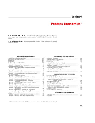
  • 6. Net annual cash income ANCI is the annual cash income ACI, minus the annual amount of tax AIT: ANCI = ACI − AIT (9-2) Taxable income is (ACI − AD − AA), where AD is the annual writing- down allowance and AA is the annual amount of any other allowances. A distinction is made between the writing-down allowance permissi- ble for the computation of tax due, the actual depreciation in value of an asset, and the book depreciation in value of that asset as shown in the company position statement. There is no necessary connection between these values unless specified by law, although the first two or all three are often assigned the same value in practice. Some govern- ments give cash incentives to encourage companies to build plants in otherwise unattractive areas. Neither AD nor AA involves any expendi- ture of cash, since they are merely book transactions. The annual amount of tax AIT is given by AIT = (ACI − AD − AA)t (9-3) where t is the fractional tax rate. The value of t is determined by the appropriate tax authority and is subject to change. For most devel- oped countries the value of t is about 0.35 or 35 percent. The annual amount of tax AIT included in Eq. (9-2) does not neces- sarily correspond to the annual cash income ACI in the same year. The tax payments in Eq. (9-2) should be those actually paid in that year. In the United States, companies pay about 80 percent of the tax on esti- mated current-year earnings in the same year. In the United King- dom, companies do not pay tax until at least 9 months after the end of the accounting period, which, for the most part, amounts to paying tax on the previous year’s earnings. When assessing projects for different countries, engineers should acquaint themselves with the tax situation in those countries. In modern methods of profitability assessment, cash flows are more meaningful than profits, which tend to be rather loosely defined. The net annual cash flow after tax is given by ACF = ANCI − ATC (9-4) where ATC is the annual expenditure of capital, which is not necessar- ily zero after the plant has been built. For example, working capital, plant additions, or modifications may be required in future years. The total annual expense ATE required to produce and sell a prod- uct can be written as the sum of the annual general expense AGE and the annual manufacturing cost or expense AME: ATE = AGE + AME (9-5) Annual general expense AGE arises from the following items: adminis- tration, sales, shipping of product, advertising and marketing, techni- cal service, research and development, and finance. The terms gross annual profit AGP and net annual profit ANP are commonly used by accountants and misused by others. Normally, both AGP and ANP are calculated before tax is deducted. Gross annual profit AGP is given by AGP = AS − AME − ABD (9-6) where ABD is the balance-sheet annual depreciation charge, which is not necessarily the same as AD used in Eq. (9-3) for tax purposes. Net annual profit ANP is simply ANP = AGP − AGE (9-7) Equation (9-7) can also be written as ANP = ACI − ABD (9-8) Net annual profit after tax ANNP can be written as ANNP = ANCI − ABD (9-9) The relationships among the various annual costs given by Eqs. (9-1) through (9-9) are illustrated diagrammatically in Fig. 9-1. The top half of the diagram shows the tools of the accountant; the bottom half, those of the engineer. The net annual cash flow ACF, which excludes any provision for balance-sheet depreciation ABD, is used in two of the more modern methods of profitability assessment: the net-present- value (NPV) method and the discounted-cash-flow-rate-of-return (DCFRR) method. In both methods, depreciation is inherently taken care of by calculations which include capital recovery. Annual general expense AGE can be written as the sum of the fixed and variable general expenses: AGE = AFGE + AVGE (9-10) Similarly, annual manufacturing expense AME can be written as the sum of the fixed and variable manufacturing expenses: AME = AFME + AVME (9-11) A variable expense is considered to be one which is directly propor- tional to the rate of production RP or of sales RS as is most appropriate to the case under consideration. Unless the variation in finished- product inventory is large when compared with the total production over the period in question, it is usually sufficiently accurate to con- sider RP and RS to be represented by the same-numerical-value R units of sale or production per year. A fixed expense is then considered to be one which is not directly proportional to R, such as overhead charges. Fixed expenses are not necessarily constant but may be sub- 9-6 PROCESS ECONOMICS FIG. 9-1 Relationship between annual costs, annual profits, and cash flows for a project. ABD = annual depreci- ation allowance; ACF = annual net cash flow after tax; ACI = annual cash income; AGE = annual general expense; AGP = annual gross profit; AIT = annual tax; AME = annual manufacturing cost; ANCI = annual net cash income; ANNP = annual net profit after taxes; ANP = annual net profit; AS = annual sales; ATC = annual total cost; (DCFRR) = discounted-cash-flow rate of return; (NPV) = net present value. Copyright © 1999 by The McGraw-Hill Companies, Inc. All rights reserved. Use of this product is subject to the terms of its license agreement. Click here to view.
  • 7. ject to stepwise variation at different levels of production. Some authors consider such steps as included in a semivariable expense, which is less amenable to mathematical analysis than the above divi- sion of expenses. Contribution and Breakeven Charts These can be used to give valuable preliminary information prior to the use of the more sophisticated and time-consuming methods based on discounted cash flow. If the sales price per unit of sales is cS and the variable expense is cVE per unit of production, Eq. (9-7) can be rewritten as ANP = R(cS − cVE) − AFE (9-12) where R(cS − cVE) is known as the annual contribution. The net annual profit is zero at an annual production rate RB = AFE/(cS − cVE) (9-13) where RB is the breakeven production rate. Breakeven charts can be plotted in any of the three forms shown in Figs. 9-2, 9-3, and 9-4. The abscissa shown as annual sales volume R is also frequently plotted as a percentage of the designed production or sales capacity R0. In the case of ships, aircraft, etc., it is then called the percentage utilization. The percentage margin of safety is defined as 100(R0 − RB)/R0. A decrease in selling price cS will decrease the slope of the lines in Figs. 9-2, 9-3, and 9-4 and increase the required breakeven value RB for a given level of fixed expense AFE. Capital Costs The total capital cost CTC of a project consists of the fixed-capital cost CFC plus the working-capital cost CWC, plus the cost of land and other nondepreciable costs CL: CTC = CFC + CWC + CL (9-14) The project may be a complete plant, an addition to an existing plant, or a plant modification. The working-capital cost of a process or a business normally includes the items shown in Table 9-1. Since working capital is com- pletely recoverable at any time, in theory if not in practice, no tax allowance is made for its depreciation. Changes in working capital arising from varying trade credits or payroll or inventory levels are usually treated as a necessary business expense except when they exceed the tax debt due. If the annual income is negative, additional working capital must be provided and included in the ATC for that year. The value of land and other nondepreciables often increases over the working life of the project. These are therefore not treated in the same way as other capital investments but are shown to have made a (taxable) profit or loss only when the capital is finally recovered. Working capital may vary from a very small fraction of the total cap- ital cost to almost the whole of the invested capital, depending on the process and the industry. For example, in jewelry-store operations, the fixed capital is very small in comparison with the working capital. On the other hand, in the chemical-process industries, the working capi- tal is likely to be in the region of 10 to 20 percent of the value of the fixed-capital investment. Depreciation The term “depreciation” is used in a number of different contexts. The most common are: 1. A tax allowance 2. A cost of operation 3. A means of building up a fund to finance plant replacement 4. A measure of falling value In the first case, the annual taxable income is reduced by an annual depreciation charge or allowance which has the effect of reducing the annual amount of tax payable. The annual depreciation charge is merely a book transaction and does not involve any expenditure of cash. The method of determining the annual depreciation charge must be agreed to by the appropriate tax authority. In the second case, depreciation is considered to be a manufactur- ing cost in the same way as labor cost or raw-materials cost. However, INVESTMENT AND PROFITABILITY 9-7 FIG. 9-2 Conventional breakeven chart. FIG. 9-3 Breakeven chart showing fixed expense as a burden cost. FIG. 9-4 Breakeven chart showing relationship between contribution and fixed expense. TABLE 9-1 Working-Capital Costs Raw materials for plant startup Raw-materials, intermediate, and finished-product inventories Cost of handling and transportation of materials to and from stores Cost of inventory control, warehouse, associated insurance, security arrangements, etc. Money to carry accounts receivable (i.e., credit extended to customers) less accounts payable (i.e., credit extended by suppliers) Money to meet payrolls when starting up Readily available cash for emergencies Any additional cash required to operate the process or business Copyright © 1999 by The McGraw-Hill Companies, Inc. All rights reserved. Use of this product is subject to the terms of its license agreement. Click here to view.
  • 8. it is more difficult to estimate a depreciation cost per unit of product than it is to do so for labor or raw-materials costs. In the net-present- value (NPV) and discounted-cash-flow-rate-of-return (DCFRR) methods of measuring profitability, depreciation, as a cost of opera- tion, is implicitly accounted for. (NPV) and (DCFRR) give measures of return after a project has generated sufficient income to repay, among other things, the original investment and any interest charges that the invested money would otherwise have brought into the company. In the third case, depreciation is considered as a means of providing for plant replacement. In the rapidly changing modern chemical- process industries, many plants will never be replaced because the processes or products have become obsolete during their working life. Management should be free to invest in the most profitable projects available, and the creation of special-purpose funds may hinder this. However, it is desirable to designate a proportion of the retained income as a fund from which to finance new capital projects. These are likely to differ substantially from the projects that originally gen- erated the income. In the fourth case, a plant or a piece of equipment has a limited use- ful life. The primary reason for the decrease in value is the decrease in future life and the consequent decrease in the number of years for which income will be earned. At the end of its life, the equipment may be worth nothing, or it may have a salvage or scrap value S. Thus a fixed-capital cost CFC depreciates in value during its useful life of s years by an amount that is equal to (CFC − S). The useful life is taken from the startup of the plant. On the basis of straight-line depreciation, the average annual amount of depreciation AD over a service life of s years is given by AD = (CFC − S)/s (9-15) The book value after the first year P1 is given by P1 = CFC − AD (9-16) The book value at the end of a specified number of years s′ is given by Ps′ = CFC − s′AD (9-17) The principal use of a particular depreciation rate is for tax pur- poses. The permitted annual depreciation is subtracted from the annual income before the latter is taxed. The basis for depreciation in a particular case is a matter of agreement between the taxation author- ity and the company, in conformity with tax laws. Other commonly used methods of computing depreciation are the declining-balance method (also known as the fixed-percentage method) and the sum-of-years-digits method. On the basis of declining-balance (fixed-percentage) depreciation, the book value at the end of the first year is given by P1 = CFC(1 − r) (9-18) where r is a fraction to be agreed with the taxation authority. The book value at the end of specified number of years s′ is given by Ps′ = CFC(1 − r)s′ (9-19) When the fraction r is chosen to be 2/s, i.e., twice the reciprocal of the service life s, the method is called the double-declining-balance method. The declining-balance method of depreciation allows equipment or plant to be depreciated by a greater amount during the earlier years than during the later years. This method does not allow equipment or plant to be depreciated to a zero value at the end of the service life. On the basis of sum-of-years-digits depreciation, the annual amount of depreciation for a specified number of years s′ for a plant of fixed-capital cost CFC, scrap value S, and service life s is given by ADs′ = 1 2(CFC − S) (9-20) Equation (9-20) can also be rewritten in the form ADs′ = 3 4(CFC − S) (9-21) 2(s − s′ + 1) }} s(s + 1) s − s′ + 1 }} 1 + 2 + 3 + ⋅ ⋅ ⋅ + s It can be shown that the book value at the end of a particular year s′ is Ps′ = 2 3 4(CFC − S) + S (9-22) The sum-of-years-digits depreciation allows equipment or plant to be depreciated by a greater amount during the early years than during the later years. A fourth method of computing depreciation (now seldom used) is the sinking-fund method. In this method, the annual depreciation AD is the same for each year of the life of the equipment or plant. The series of equal amounts of depreciation AD, invested at a fractional interest rate i and made at the end of each year over the life of the equipment or plant of s years, is used to build up a future sum of money equal to (CFC − S). This last is the fixed-capital cost of the equipment or plant minus its salvage or scrap value and is the total amount of depreciation during its useful life. The equation relating (CFC − S) and AD is simply the annual cost or payment equation, writ- ten either as CFC − S = AD 3 4 (9-23) or CFC − S = (9-24) where fAF is the annuity future-worth factor given by fAF = i/[(1 + i)s − 1] In the sinking-fund method of depreciation, the effect of interest is to make the annual decrease of the book value of the equipment or plant less in the early than in the later years with consequent higher tax due in the earlier years when recovery of the capital is most impor- tant. It is preferable not to think of annual depreciation as a contribution to a fund to replace equipment at the end of its life but as part of the difference between the revenue and the expenditure, which differ- ence is tax-free. Some of the preceding methods of computing depreciation are not allowed by taxation authorities in certain countries. When calculating depreciation, it is necessary to obtain details of the methods and rates permitted by the appropriate authority and to use the information provided. Figure 9-5 shows the fall in book value with time for a piece of equipment having a fixed-capital cost of $120,000, a useful life of 10 years, and a scrap value of $20,000. This fall in value is calculated by using (1) straight-line depreciation, (2) double-declining depreciation, and (3) sum-of-years-digits depreciation. Traditional Measures of Profitability Rate-of-Return Methods Although traditional rate-of-return methods have the advantage of simplicity, they can yield very mislead- ing results. They are based on the relation Percent rate of return = [(annual profit)/(invested capital)]100 (9-25) Since different meanings are ascribed to both annual profit and invested capital in Eq. (9-25), it is important to define the terms pre- cisely. The invested capital may refer to the original total capital investment, the depreciated investment, the average investment, the current value of the investment, or something else. The annual profit may refer to the net annual profit before tax ANP, the net annual profit after tax ANNP, the annual cash income before tax ACI, or the annual cash income after tax ANCI. The fractional interest rate of return based on the net annual profit after tax and the original investment is i = ANNP /CTC (9-26) which can be written in terms of Eq. (9-9) as i = (ANCI /CTC) − (ABD /CTC) (9-27) where ABD is the balance-sheet annual depreciation. The main disad- vantage of using Eq. (9-27) is that the fractional depreciation rate AD } fAF (1 + i)s − 1 }} i 1 + 2 + ⋅ ⋅ ⋅ + (s − s′) }}} s(s + 1) 9-8 PROCESS ECONOMICS Copyright © 1999 by The McGraw-Hill Companies, Inc. All rights reserved. Use of this product is subject to the terms of its license agreement. Click here to view.
  • 9. ABD /CTC is arbitrarily assessed. Its value will affect the fractional rate of return considerably and may lead to erroneous conclusions when making comparisons between different companies. This is particularly true when making international comparisons. Figures 9-6, 9-7, and 9-8 show the effect of the depreciation method on profit for a project described by the following data: Net annual cash income after tax ANCI = $25,500 in each of 10 years Fixed-capital cost CFC = $120,000 Estimated salvage value of plant items S = $20,000 Working capital CWC = $10,000 Cost of land CL = $20,000 In Eq. (9-27), i can be taken either on the basis of the net annual cash income for a particular year or on the basis of an average net annual cash income over the length of the life of the project. The equations corresponding to Eq. (9-26) based on depreciated and aver- age investment are given respectively as follows: i = ANNP /(Ps′ + CWC + CL) (9-28) and i = 2ANNP /(CFC + S + 2CWC + 2CL) (9-29) INVESTMENT AND PROFITABILITY 9-9 FIG. 9-5 Book value against time for various depreciation methods. FIG. 9-6 Effect of straight-line depreciation on rate of return for a project. ABD = annual depreciation allowance; ANCI = annual net cash income after tax; ANNP = annual net profit after payment of tax; CTC = total capital cost. FIG. 9-7 Effect of double-declining depreciation on rate of return for a proj- ect. FIG. 9-8 Effect of sum-of-years-digits depreciation on rate of return for a project. Copyright © 1999 by The McGraw-Hill Companies, Inc. All rights reserved. Use of this product is subject to the terms of its license agreement. Click here to view.
  • 10. where Ps′ is the book value of the fixed-capital investment at the end of a particular year s′. If i is taken on the basis of average values for ANNP over the length of the project, an average value for the working capital CWC must be used. In Eqs. (9-28) and (9-29), the computations are based on unchang- ing values of the cost of land and other nondepreciable costs CL. This is unrealistic, since the value of land has a tendency to rise. In such cir- cumstances, the accountancy principle of conservatism requires that the lowest valuation be adopted. Payback Period Another traditional method of measuring prof- itability is the payback period or fixed-capital-return period. Actually, this is really a measure not of profitability but of the time it takes for cash flows to recoup the original fixed-capital expenditure. The net annual cash flow after tax is given by ACF = ANCI − ATC (9-4) where ATC is the annual expenditure of capital, which is not necessar- ily zero after the plant has been built. The payback period (PBP) is the time required for the cumulative net cash flow taken from the startup of the plant to equal the depreciable fixed-capital investment (CFC − S). It is the value of s′ that satisfies ^ s′ = (PBP) s′ = 0 ACF = CFC − S (9-30) The payback-period method takes no account of cash flows or prof- its received after the breakeven point has been reached. The method is based on the premise that the earlier the fixed capital is recovered, the better the project. However, this approach can be misleading. Let us consider projects A and B, having net annual cash flows as listed in Table 9-2. Both projects have initial fixed-capital expendi- tures of $100,000. On the basis of payback period, project A is the more desirable since the fixed-capital expenditure is recovered in 3 years, compared with 5 years for project B. However, project B runs for 7 years with a cumulative net cash flow of $110,000. This is obvi- ously more profitable than project A, which runs for only 4 years with a cumulative net cash flow of only $10,000. Time Value of Money A large part of business activity is based on money that can be loaned or borrowed. When money is loaned, there is always a risk that it may not be returned. A sum of money called interest is the inducement offered to make the risk acceptable. When money is borrowed, interest is paid for the use of the money over a period of time. Conversely, when money is loaned, interest is received. The amount of a loan is known as the principal. The longer the period of time for which the principal is loaned, the greater the total amount of interest paid. Thus, the future worth of the money F is greater than its present worth P. The relationship between F and P depends on the type of interest used. Table 9-3 gives examples of compound-interest factors and example compound-interest calculations. Simple Interest When simple interest is used, F and P are related by F = P(1 + ni) (9-31) where i is the fractional interest rate per period and n is the number of interest periods. Normally, the interest period is 1 year, in which case i is known as the effective interest rate. Annual Compound Interest It is more common to use com- pound interest, in which F and P are related by F = P(1 + i)n (9-32) or F = Pfi (9-33) where the compound-interest factor fi = (1 + i)n . Values for com- pound-interest factors are readily available in tables. The present value P of a future sum of money F is P = F/(1 + i)n (9-34) or F = P/fd (9-35) where the discount factor fd is fd = 1/fi = 1/[(1 + i)n ] Values for the discount factors are readily available in tables which show that it will take 7.3 years for the principal to double in amount if compounded annually at 10 percent per year and 14.2 years if com- pounded annually at 5 percent per year. For the case of different annual fractional interest rates (i1,i2, . . . ,in in successive years), Eq. (9-32) should be written in the form F = P(1 + i1)(1 + i2)(1 + i3) ⋅ ⋅ ⋅ (1 + in) (9-36) Short-Interval Compound Interest If interest payments become due m times per year at compound interest, mn payments are required in n years. The nominal annual interest rate i′ is divided by m to give the effective interest rate per period. Hence, F = P[1 + (i′/m)]mn (9-37) It follows that the effective annual interest i is given by i = [1 + (i′/m)]m − 1 (9-38) The annual interest rate equivalent to a compound-interest rate of 5 percent per month (i.e., i′/m = 0.05) is calculated from Eq. (9-38) to be i = (1 + 0.05)12 − 1 = 0.796, or 79.6 percent/year Continuous Compound Interest As m approaches infinity, the time interval between payments becomes infinitesimally small, and in the limit Eq. (9-37) reduces to F = P exp (i′n) (9-39) A comparison of Eqs. (9-32) and (9-39) shows that the nominal interest rate i′ on a continuous basis is related to the effective interest rate i on an annual basis by exp (i′n) = (1 + i)n (9-40) Numerically, the difference between continuous and annual com- pounding is small. In practice, it is probably far smaller than the errors in the estimated cash-flow data. Annual compound interest conforms more closely to current acceptable accounting practice. However, the small difference between continuous and annual compounding may be significant when applied to very large sums of money. Let us suppose that $100 is invested at a nominal interest rate of 5 percent. We then compute the future worth of the investment after 2 years and also compute the effective annual interest rate for the fol- lowing kinds of interest: (1) simple, (2) annual compound, (3) monthly compound, (4) daily compound, and (5) continuous compound. The following tabulation shows the results of the calculations, along with the appropriate equation to be used: Interest Future Effective type Equation worth F rate i, % Equation 1 (9-31) $110.000 5 (9-31) 2 (9-32) $110.250 5 (9-38) 3 (9-37) $110.495 5.117 (9-38) 4 (9-37) $110.516 5.1267 (9-38) 5 (9-39) $110.517 5.1271 (9-38) When computing the effective annual rate for continuous com- pounding, the first term of Eq. (9-38), [1 + (i′/m)]m , approaches ei′ as m approaches infinity. 9-10 PROCESS ECONOMICS TABLE 9-2 Cash Flows for Two Projects Cash flows ACF Year Project A Project B 0 $100,000 $100,000 1 50,000 0 2 30,000 10,000 3 20,000 20,000 4 10,000 30,000 5 0 40,000 6 0 50,000 7 0 60,000 ^ ACF $ 10,000 $110,000 Payback period (PBP) 3 years 5 years Copyright © 1999 by The McGraw-Hill Companies, Inc. All rights reserved. Use of this product is subject to the terms of its license agreement. Click here to view.
  • 11. 9-11 TABLE 9-3 Compound Interest Factors* (For examples demonstrating use see end of table.) Single payment Uniform annual series Single payment Uniform annual series Compound- Present- Sinking- Capital- Compound- Present- Compound- Present- Sinking- Capital- Compound- Present- amount worth fund recovery amount worth amount worth fund recovery amount worth factor factor factor factor factor factor factor factor factor factor factor factor Given P, Given F, Given F, Given P, Given A, Given A, Given P, Given F, Given F, Given P, Given A, Given A, to find F to find P to find A to find A to find F to find P to find F to find P to find A to find A to find F to find P n (1 + i)n (1 + i)n n 5% Compound Interest Factors 6% Compound Interest Factors 1 1.050 0.9524 1.00000 1.05000 1.000 0.952 1.060 0.9434 1.00000 1.06000 1.000 0.943 1 2 1.103 .9070 0.48780 0.53780 2.050 1.859 1.124 .8900 0.48544 0.54544 2.060 1.833 2 3 1.158 .8638 .31721 .36721 3.153 2.723 1.191 .8396 .31411 .37411 3.184 2.673 3 4 1.216 .8227 .23201 .28201 4.310 3.546 1.262 .7921 .22859 .28859 4.375 3.465 4 5 1.276 .7835 .18097 .23097 5.526 4.329 1.338 .7473 .17740 .23740 5.637 4.212 5 6 1.340 .7462 .14702 .19702 6.802 5.076 1.419 .7050 .14336 .20336 6.975 4.917 6 7 1.407 .7107 .12282 .17282 8.142 5.786 1.504 .6651 .11914 .17914 8.394 5.582 7 8 1.477 .6768 .10472 .15472 9.549 6.463 1.594 .6274 .10104 .16104 9.897 6.210 8 9 1.551 .6446 .09069 .14069 11.027 7.108 1.689 .5919 .08702 .14702 11.491 6.802 9 10 1.629 .6139 .07940 .12950 12.578 7.722 1.791 .5584 .07587 .13587 13.181 7.360 10 11 1.710 .5847 .07039 .12039 14.207 8.306 1.898 .5268 .06679 .12679 14.972 7.887 11 12 1.796 .5568 .06283 .11283 15.917 8.863 2.012 .4970 .05928 .11928 16.870 8.384 12 13 1.886 .5303 .05646 .10646 17.713 9.394 2.133 .4688 .05296 .11296 18.882 8.853 13 14 1.980 .5051 .05102 .10102 19.599 9.899 2.261 .4423 .04758 .10758 21.015 9.295 14 15 2.079 .4810 .04634 .09634 21.579 10.380 2.397 .4173 .04296 .10296 23.276 9.712 15 16 2.183 .4581 .04227 .09227 23.657 10.838 2.540 .3936 .03895 .09895 25.673 10.106 16 17 2.292 .4363 .03870 .08870 25.840 11.274 2.693 .3714 .03544 .09544 28.213 10.477 17 18 2.407 .4155 .03555 .08555 28.132 11.690 2.854 .3503 .03236 .09236 30.906 10.828 18 19 2.527 .3957 .03275 .08275 30.539 12.085 3.026 .3305 .02962 .08962 33.760 11.158 19 20 2.653 .3769 .03024 .08024 33.066 12.462 3.207 .3118 .02718 .08718 36.786 11.470 20 21 2.786 .3589 .02800 .07800 35.719 12.821 3.400 .2942 .02500 .08500 39.993 11.764 21 22 2.925 .3418 .02597 .07597 38.505 13.163 3.604 .2775 .02305 .08305 43.392 12.042 22 23 3.072 .3256 .02414 .07414 41.430 13.489 3.820 .2618 .02128 .08128 46.996 12.303 23 24 3.225 .3101 .02247 .07247 44.502 13.799 4.049 .2470 .01968 .07968 50.816 12.550 24 25 3.386 .2953 .02095 .07095 47.727 14.094 4.292 .2330 .01823 .07823 54.865 12.783 25 26 3.556 .2812 .01956 .06956 51.113 14.375 4.549 .2198 .01690 .07690 59.156 13.003 26 27 3.733 .2678 .01829 .06829 54.669 14.643 4.822 .2074 .01570 .07570 63.706 13.211 27 28 3.920 .2551 .01712 .06712 58.403 14.898 5.112 .1956 .01459 .07459 68.528 13.406 28 29 4.116 .2429 .01605 .06605 62.323 15.141 5.418 .1846 .01358 .07358 73.640 13.591 29 30 4.322 .2314 .01505 .06505 66.489 15.372 5.743 .1741 .01265 .07265 79.058 13.765 30 31 4.538 .2204 .01413 .06413 70.761 15.593 6.088 .1643 .01179 .07179 84.802 13.929 31 32 4.765 .2099 .01328 .06328 75.299 15.803 6.453 .1550 .01100 .07100 90.890 14.084 32 33 5.003 .1999 .01249 .06249 80.064 16.003 6.841 .1462 .01027 .07027 97.343 14.230 33 34 5.253 .1904 .01176 .06176 85.067 16.193 7.251 .1379 .00960 .06960 104.184 14.368 34 35 5.516 .1813 .01107 .06107 90.320 16.374 7.686 .1301 .00897 .06897 111.435 14.498 35 40 7.040 .1420 .00828 .05828 120.800 17.159 10.286 .0972 .00646 .06646 154.762 15.046 40 45 8.985 .1113 .00626 .05626 159.700 17.774 13.765 .0727 .00470 .06470 212.744 15.456 45 50 11.467 .0872 .00478 .05478 209.348 18.256 18.420 .0543 .00344 .06344 290.336 15.762 50 55 14.636 .0683 .00367 .05367 272.713 18.633 24.650 .0406 .00254 .06254 394.172 15.991 55 60 18.679 .0535 .00283 .05283 353.584 18.929 32.988 .0303 .00188 .06188 533.128 16.161 60 65 23.840 .0419 .00219 .05219 456.798 19.161 44.145 .0227 .00139 .06139 719.083 16.289 65 70 30.426 .0329 .00170 .05170 588.529 19.343 59.076 .0169 .00103 .06103 967.932 16.385 70 75 38.833 .0258 .00132 .05132 756.654 19.485 79.057 .0126 .00077 .06077 1,300.949 16.456 75 80 49.561 .0202 .00103 .05103 971.229 19.596 105.796 .0095 .00057 .06057 1,746.600 16.509 80 85 63.254 .0158 .00080 .05080 1,245.087 19.684 141.579 .0071 .00043 .06043 2,342.982 16.549 85 90 80.730 .0124 .00063 .05063 1,594.607 19.752 189.465 .0053 .00032 .06032 3,141.075 16.579 90 95 103.035 .0097 .00049 2,040.694 19.806 253.546 .0039 .00024 .06024 4,209.104 16.601 95 100 131.501 .0076 .00038 .05038 2,610.025 19.848 339.302 .0029 .00018 .06018 5,638.368 16.618 100 (1 + i)n − 1 }} i(1 + i)n (1 + i)n − 1 }} i i(1 + i)n }} (1 + i)n − 1 i }} (1 + i)n − 1 1 } (1 + i)n (1 + i)n − 1 }} i(1 + i)n (1 + i)n − 1 }} i i(1 + i)n }} (1 + i)n − 1 i }} (1 + i)n − 1 1 } (1 + i)n Copyright © 1999 by The McGraw-Hill Companies, Inc. All rights reserved. Use of this product is subject to the terms of its license agreement. Click here to view.
  • 12. 9-12 PROCESS ECONOMICS TABLE 9-3 Compound Interest Factors (Concluded) Examples of Use of Table and Factors Given: $2500 is invested now at 5 percent. Required: Accumulated value in 10 years (i.e., the amount of a given principal). Solution: F = P(1 + i)n = $2500 × 1.0510 Compound-amount factor = (1 + i)n = 1.0510 = 1.629 F = $2500 × 1.629 = $4062.50 Given: $19,500 will be required in 5 years to replace equipment now in use. Required: With interest available at 3 percent, what sum must be deposited in the bank at present to provide the required capital (i.e., the principal which will amount to a given sum)? Solution: P = F = $19,500 Present-worth factor = 1/(1 + i)n = 1/1.035 = 0.8626 P = $19,500 × 0.8626 = $16,821 Given: $50,000 will be required in 10 years to purchase equipment. Required: With interest available at 4 percent, what sum must be deposited each year to provide the required capital (i.e., the annuity which will amount to a given fund)? Solution: A = F = $50,000 Sinking-fund factor = = = 0.08329 A = $50,000 × 0.08329 = $4,164 Given: $20,000 is invested at 10 percent interest. Required: Annual sum that can be withdrawn over a 20-year period (i.e., the annuity provided by a given capital). Solution: A = P = $20,000 Capital-recovery factor = = = 0.11746 A = $20,000 × 0.11746 = $2349.20 Given: $500 is invested each year at 8 percent interest. Required: Accumulated value in 15 years (i.e., amount of an annuity). Solution: F = A = $500 Compound-amount factor = = = 27.152 F = $500 × 27.152 = $13,576 Given: $8000 is required annually for 25 years. Required: Sum that must be deposited now at 6 percent interest. Solution: P = A = $8000 Present-worth factor = = = 12.783 P = $8000 × 12.783 = $102,264 *Factors presented for two interest rates only. By using the appropriate formulas, values for other interest rates may be calculated. 1.0625 − 1 }} 0.06 × 1.0625 (1 + i)n − 1 }} i(1 + i)n 1.0625 − 1 }} 0.06 × 1.0625 (1 + i)n − 1 }} i(1 + i)n 1.0815 − 1 }} 0.08 (1 − i)n − 1 }} i 1.0815 − 1 }} 0.08 (1 + i)n − 1 }} i 0.10 × 1.1020 }} 1.1020 − 1 i(1 + i)n }} (1 + i)n − 1 0.10 × 1.1020 }} 1.1020 − 1 i(1 + i)n }} (1 + i)n − 1 0.04 }} 1.0410 − 1 i }} (1 + i)n − 1 0.04 }} 1.0410 − 1 i }} (1 + i)n − 1 1 } 1.035 1 } (1 + i)n Copyright © 1999 by The McGraw-Hill Companies, Inc. All rights reserved. Use of this product is subject to the terms of its license agreement. Click here to view.
  • 13. Annual Cost or Payment A series of equal annual payments A invested at a fractional interest rate i at the end of each year over a period of n years may be used to build up a future sum of money F. These relations are given by F = A 3 4 (9-41) or F = A/fAF (9-42) where the annuity future-worth factor is fAF = i/[(1 + i)n − 1] Values for fAF are readily available in tables. Equation (9-41) can be combined with Eq. (9-34) to yield P = A 3 4 (9-43) P = A/fAP (9-44) where P is the present worth of the series of future equal annual pay- ments A and the annuity present-worth factor is fAP = [i(1 + i)n ]/[(1 + i)n − 1] Values for fAP are also available in tables. Alternatively, the annual payment A required to build up a future sum of money F with a present value of P is given by A = FfAF (9-45) A = PfAP (9-46) Equation (9-41) represents the future sum of a series of uniform annual payments that are invested at a stated interest rate over a period of years. This procedure defines an ordinary annuity. Other forms of annuities include the annuity due, in which payments are made at the beginning of the year instead of at the end; and the deferred annuity, in which the first payment is deferred for a definite number of years. Capitalized Cost A piece of equipment of fixed-capital cost CFC will have a finite life of n years. The capitalized cost of the equipment CK is defined by (CK − CFC)(1 + i)n = CK − S (9-47) CK is in excess of CFC by an amount which, when compounded at an annual interest rate i for n years, will have a future worth of CK less the salvage or scrap value S. If the renewal cost of the equipment remains constant at (CFC − S) and the interest rate remains constant at i, then CK is the amount of capital required to replace the equipment in per- petuity. Equation (9-47) may be rewritten as CK = 3CFC − 43 4 (9-48) or CK = (CFC − Sfd)fk (9-49) where fd is the discount factor and fk, the capitalized-cost factor, is fk = [(1 + i)n ]/[(1 + i)n − 1] Values for each factor are available in tables. Example 1: Capitalized Cost of Equipment A piece of equipment has been installed at a cost of $100,000 and is expected to have a working life of 10 years with a scrap value of $20,000. Let us calculate the capitalized cost of the equipment based on an annual compound-interest rate of 5 percent. Therefore, we substitute values into Eq. (9-48) to give CK = 3$100,000 − 43 4 CK = [$100,000 − ($20,000/1.62889)](2.59009) CK = $227,207 Modern Measures of Profitability An investment in a manu- facturing process must earn more than the cost of capital for it to be worthwhile. The larger the additional earnings, the more profitable (1 + 0.05)10 }} (1 + 0.05)10 − 1 $20,000 }} (1 + 0.05)10 (1 + i)n }} (1 + i)n − 1 S } (1 + i)n (1 + i)n − 1 }} i(1 + i)n (1 + i)n − 1 }} i the venture and the greater the justification for putting the capital at risk. A profitability estimate is an attempt to quantify the desirability of taking this risk. The ways of assessing profitability to be considered in this section are (1) discounted-cash-flow rate of return (DCFRR), (2) net present value (NPV) based on a particular discount rate, (3) equivalent maxi- mum investment period (EMIP), (4) interest-recovery period (IRP), and (5) discounted breakeven point (DBEP). Cash Flow Let us consider a project in which CFC = $1,000,000, CWC = $90,000, and CL = $10,000. Hence, CTC = $1,100,000 from Eq. (9-14). If all this capital expenditure occurs in Year 0 of the project, then ATC = $1,100,000 in Year 0 and −ATC = −$1,100,000. From Eq. (9-4), it is seen that any capital expenditure makes a negative contri- bution to the net annual cash flow ACF. Let us consider another project in which the fixed-capital expendi- ture is spread over 2 years, according to the following pattern: CFC = CFC0 + CFC1 Year 0 Year 1 CFC0 = $400,000 CFC1 = $600,000 CL = 10,000 CWC = 90,000 ATC = 410,000 ATC = 690,000 In the final year of the project, the working capital and the land are recovered, which in this case cost a total of $100,000. Thus, in the final year of the project, ATC = −$100,000 and −ATC = +$100,000. From Eq. (9-4), it is seen that any capital recovery makes a positive contribution to the net annual cash flow. During the development and construction stages of a project, ACI and AIT are both zero in Eqs. (9-2) and (9-4). For this period, the cash flow for the project is negative and is given by ACF = −ATC (9-50) Figure 9-9 shows the cash-flow stages in a project. The expenditure during the research and development stage is normally relatively small. It will usually include some preliminary process design and a market survey. Once the decision to go ahead with the project has been taken, detailed process-engineering design will commence, and the rate of expenditure starts to increase. The rate is increased still further when equipment is purchased and construction gets under way. There is no return on the investment until the plant is started up. Even during startup, there is some additional expenditure. Once the plant is operating smoothly, an inflow of cash is established. During the early stages of a project, there may be a tax credit because of the existence of expenses without corresponding income. Discounted Cash Flow The present value P of a future sum of money F is given by P = Ffd (9-51) where fd = 1/(1 + i)n , the discount factor. Values for this factor are read- ily available in tables. For example, $90,909 invested at an annual interest rate of 10 percent becomes $100,000 after 1 year. Similarly, $38,554 invested at 10 percent becomes $100,000 after 10 years. Thus, cash flow in the early years of a project has a greater value than the same amount in the later years of a project. Therefore, it pays to receive money as soon as possible and to delay paying out money for as long as possible. Time is taken into account by using the annual discounted cash flow ADCF, which is related to the annual cash flow ACF and the discount fac- tor fd by ADCF = ACF fd (9-52) Thus, at the end of any year n, (ADCF)n = (ACF)n /(1 + i)n The sum of the annual discounted cash flows over n years, ^ ADCF, is known as the net present value (NPV) of the project: (NPV) = ^ n 0 (ADCF)n (9-53) INVESTMENT AND PROFITABILITY 9-13 Copyright © 1999 by The McGraw-Hill Companies, Inc. All rights reserved. Use of this product is subject to the terms of its license agreement. Click here to view.
  • 14. The value of (NPV) is directly dependent on the choice of the frac- tional interest rate i. An interest rate can be selected to make (NPV) = 0 after a chosen number of years. This value of i is found from ^ n 0 (ADCF)n = + + ⋅ ⋅ ⋅ + = 0 (9-54) Equation (9-54) may be solved for i either graphically or by an iter- ative trial-and-error procedure. The value of i given by Eq. (9-54) is known as the discounted-cash-flow rate of return (DCFRR). It is also known as the profitability index, true rate of return, investor’s rate of return, and interest rate of return. Cash-Flow Curves Figure 9-9 shows the cash-flow stages in a project together with their discounted-cash-flow values for the data given in Table 9-4. In addition to cash-flow and discounted-cash-flow curves, it is also instructive to plot cumulative-cash-flow and cumula- tive-discounted-cash-flow curves. These are shown in Fig. 9-10 for the data in Table 9-4. The cost of capital may also be considered as the interest rate at which money can be invested instead of putting it at risk in a manu- facturing process. Let us consider the process data listed in Table 9-4 and plotted in Fig. 9-10. If the cost of capital is 10 percent, then the appropriate discounted-cash-flow curve in Fig. 9-10 is abcdef. Up to point e, or 8.49 years, the capital is at risk. Point e is the discounted breakeven point (DBEP). At this point, the manufacturing process (ACF)n } (1 + i)n (ACF)1 } (1 + i)1 (ACF)0 } (1 + i)0 has paid back its capital and produced the same return as an equiva- lent amount of capital invested at a compound-interest rate of 10 per- cent. Beyond the breakeven point, the capital is no longer at risk and any cash flow above the horizontal baseline, ^ADCF = 0, is in excess of the return on an equivalent amount of capital invested at a compound- interest rate of 10 percent. Thus, the greater the area above the base- line, the more profitable the process. When (NPV) and (DCFRR) are computed, depreciation is not con- sidered as a separate expense. It is simply used as a permitted writing- down allowance to reduce the annual amount of tax in accordance with the rules applying in the country of earning. The tax payable is deducted in accordance with Eq. (9-2) in the year in which it is paid, which may differ from the year in which the corresponding income was earned. A (DCFRR) of, say, 15 percent implies that 15 percent per year will be earned on the investment, in addition to which the project gener- ates sufficient money to repay the original investment plus any inter- est payable on borrowed capital plus all taxes and expenses. It is not normally possible to make a comprehensive assessment of profitability with a single number. The shape of the cumulative-cash- flow and cumulative-discounted-cash-flow curves both before and after the breakeven point is an important factor. D. H. Allen [Chem. Eng., 74, 75–78 (July 3, 1967)] accounted for the shape of the cumulative-undiscounted-cash-flow curve up to the 9-14 PROCESS ECONOMICS FIG. 9-9 Effect of discount rate on cash flows. TABLE 9-4 Annual Cash Flows and Discounted Cash Flows for a Project Discounted at 10% Discounted at 20% Discounted at 25% Year ACF, $ ^ ACF, $ fd ADCF, $ ^ ADCF, $ fd ADCF, $ ^ ADCF, $ fd ADCF, $ ^ ADCF, $ 0 −10,000 −10,000 1.00000 −10,000 −10,000 1.00000 −10,000 −10,000 1.00000 −10,000 −10,000 1 −30,000 −40,000 0.90909 −27,273 −37,273 0.83333 −25,000 −35,000 0.80000 −24,000 −34,000 2 −60,000 −100,000 0.82645 −49,587 −86,860 0.69444 −41,666 −76,666 0.64000 −38,400 −72,400 3 −750,000 −850,000 0.75131 −563,483 −650,343 0.57870 −434,025 −510,691 0.51200 −384,000 −456,400 4 −150,000 −1,000,000 0.68301 −102,452 −752,795 0.48225 −72,338 −583,029 0.40960 −61,440 −517,840 5 +200,000 −800,000 0.62092 +124,184 −628,611 0.40188 +80,376 −502,653 0.32768 +65,536 −452,304 6 +300,000 −500,000 0.56447 +169,341 −459,270 0.33490 +100,470 −402,183 0.26214 +78,642 −373,662 7 +400,000 −100,000 0.51316 +205,264 −254,006 0.27908 +111,632 −290,551 0.20972 +83,888 −289,774 8 +400,000 +300,000 0.46651 +186,604 −67,402 0.23257 +93,028 −197,523 0.16777 +67,108 −222,666 9 +360,000 +660,000 0.42410 +152,676 +85,274 0.19381 +69,772 −127,751 0.13422 +48,319 −174,347 10 +320,000 +980,000 0.38554 +123,373 +208,647 0.16151 +51,683 −76,068 0.10737 +34,358 −139,989 11 +280,000 +1,260,000 0.35049 +98,137 +306,784 0.13459 +37,685 −38,383 0.08590 +24,052 −115,937 12 +240,000 +1,500,000 0.31863 +76,471 +383,255 0.11216 +26,918 −11,465 0.06872 +16,493 −99,444 13 +240,000 +1,740,000 0.28966 +69,518 +452,773 0.09346 +22,430 +10,965 0.05498 +13,195 −86,249 14 +400,000 +2,140,000 0.26333 +105,332 +558,105 0.07789 +31,156 +42,121 0.04398 +17,592 −68,657 NOTE: ACF is net annual cash flow, ADCF is net annual discounted cash flow, fd is discount factor at stated interest, ^ ACF is cumulative cash flow, and ^ ADCF is cumu- lative discounted cash flow. Copyright © 1999 by The McGraw-Hill Companies, Inc. All rights reserved. Use of this product is subject to the terms of its license agreement. Click here to view.
  • 15. breakeven point e0 in Fig. 9-10 by using a parameter known as the equivalent maximum investment period (EMIP), which is defined as (EMIP) = for ACF ≤ 0 (9-55) where the area (a0 to e0) refers to the area below the horizontal base- line (^ ACF = 0) on the cumulative-cash-flow curve in Fig. 9-10. The sum (^ ACF)max is the maximum cumulative expenditure on the proj- ect, which is given by point d0 in Fig. 9-10. (EMIP) is a time in years. It is the equivalent period during which the total project debt would be outstanding if it were all incurred at one instant and all repaid at one instant. Clearly, the shorter the (EMIP), the more attractive the project. Allen accounted for the shape of the cumulative-cash-flow curve area (a0 to e0) }} (^ ACF)max beyond the breakeven point by using a parameter known as the inter- est-recovery period (IRP). This is the time period (illustrated in Fig. 9-11) that makes the area (e0 to f0) above the horizontal baseline equal to the area (a0 to e0) below the horizontal baseline on the cumulative- cash-flow curve. C. G. Sinclair [Chem. Process. Eng., 47, 147 (1966)] has considered similar parameters to the (EMIP) and (IRP) based on a cumulative- discounted-cash-flow curve. Consideration of the cash-flow stages in Fig. 9-10 shows the factors that can affect the (EMIP) and (IRP). If the required capital invest- ment is increased, it is necessary to increase the rate of income after startup for the (EMIP) to remain the same. In order to have the (EMIP) small, it is necessary to keep the research and development, design, and construction stages short. INVESTMENT AND PROFITABILITY 9-15 FIG. 9-10 Effect of discount rate on cumulative cash flows. FIG. 9-11 Cumulative cash flow against time, showing interest recovery period. Copyright © 1999 by The McGraw-Hill Companies, Inc. All rights reserved. Use of this product is subject to the terms of its license agreement. Click here to view.
  • 16. Example 2: Net Present Value for Different Depreciation Methods The following data describe a project. Revenue from annual sales and the total annual expense over a 10-year period are given in the first three columns of Table 9-5. The fixed-capital investment CFC is $1,000,000. Plant items have a zero salvage value. Working capital CWC is $90,000, and cost of land CL is $10,000. There are no tax allowances other than depreciation; i.e., AA is zero. The fractional tax rate t is 0.50. We shall calculate for these data the net present value (NPV) for the follow- ing depreciation methods and discount factors: a. Straight-line, 10 percent b. Straight-line, 20 percent c. Double-declining, 10 percent d. Sum-of-years-digits, 10 percent e. Straight-line, 10 percent; income tax delayed for 1 year In addition, we shall calculate the discounted-cash-flow rate of return (DCFRR) with straight-line depreciation. a. We begin the calculations for this example by finding the total capital cost CTC for the project from Eq. (9-14). Here, CTC = $1,100,000. In Year 0, this amount is the same as the net annual capital expenditure ATC and is listed in Table 9-5. The annual rate of straight-line depreciation of the fixed-capital investment CFC, from $1,000,000 at startup to a salvage value S, of zero at the end of a pro- ductive life s of 10 years, is given by AD = (CFC − S)/s AD = ($1,000,000 − $0)/10 years = $100,000/year The annual cash income ACI for Year 1, when AS = $400,000 per year and ATE = $100,000 per year, is, from Eq. (9-1), $300,000 per year. Values for subse- quent years are calculated in the same way and listed in Table 9-4. Annual amount of tax AIT for Year 1, when ACI = $300,000 per year, AD = $100,000 per year, AA = $0 per year, and t = 0.5, is found from Eq. (9-3) to be AIT = [($300,000 − $100,000 − $0)/year](0.5) = $100,000/year Values for subsequent years are calculated in the same way and listed in Table 9-4. Net annual cash flow (after tax) ACF for Year 0, when ACI = $0 per year, AIT = $0 per year, and ATC = $1,100,000 per year, is found from Eq. (9-4) to be ACF = $0/year − $1,100,000/year = −$1,100,000/year Net annual cash flow (after tax) ACF for Year 1, when ACI = $300,000 per year, AIT = $100,000 per year, and ATC = $0 per year, is found from Eqs. (9-2) and (9-4) to be ACF = $200,000/year − $0/year = $200,000/year Values for the years up to and including Year 9 are calculated in the same way and listed in Table 9-5. At the end of Year 10, the working capital (CWC = $90,000) and the cost of land (CL = $10,000) are recovered, so that the annual expenditure of capital ATC in Year 10 is −$100,000 per year. Hence, the net annual cash flow (after tax) for Year 10 must reflect this recovery. By using Eq. (9-4), ACF = $110,000/year − (−$100,000/year) = $210,000/year The net annual discounted cash flow ADCF for Year 1, when ACF = $200,000 per year and fd = 0.90909 (for i = 10 percent), is found from Eq. (9-52) to be ADCF = ($200,000/year)(0.90909) = $181,820/year Values for subsequent years are calculated in the same way and listed in Table 9-5. The net present value (NPV) is found by summing the values of ADCF for each year, as in Eq. (9-53). The net present value is found to be $276,210, as given by the final entry in Table 9-5. b. The same procedure is used for i = 20 percent. The discount factors to be used in a table similar to Table 9-5 must be those for 20 percent. The (NPV) is found to be −$151,020. c. The calculations are similar to those for subexample a except that depre- ciation is computed by using the double-declining method of Eq. (9-19). The net present value is found to be $288,530. d. Again, the calculations are similar to those for subexample a except that depreciation is computed by using the sum-of-years-digits method of Eq. (9-20). The net present value is found to be $316,610. e. The calculations follow the same procedure as for subexample a, but the annual amount of tax AIT is calculated for a particular year and then deducted from the annual cash income ACI for the following year. The net present value for Year 11 is found to be $341,980. The discounted-cash-flow rate of return (DCFRR) can readily be obtained approximately by interpolation of the (NPV) for i = 10 percent and i = 20 per- cent: (DCFRR) = 0.100 + [($276,210)(0.20 − 0.10)]/[$276,210 − (−$151,020)] (DCFRR) = 0.164, or 16.4 percent The calculation of (DCFRR) usually requires a trial-and-error solution of Eq. (9-57), but rapidly convergent methods are available [N. H. Wild, Chem. Eng., 83, 153–154 (Apr. 12, 1976)]. For simplicity linear interpolation is often used. A comparison of the (NPV) values for a 10 percent discount factor shows clearly that double-declining depreciation is more advantageous than straight- line depreciation and that sum-of-years-digits depreciation is more advanta- geous than the double-declining method. However, a significant advantage is obtained by delaying the payment of tax for 1 year even with straight-line depre- ciation. This example is a simplified one. The cost of the working capital is assumed to be paid for in Year 0 and returned in Year 10. In practice, working capital increases with the production rate. Thus there may be an annual expenditure on working capital in a number of years subse- quent to Year 0. Except in loss-making years, this is usually treated as an expense of the process. In loss-making years the cash injection for working capital is included in the ATC for that year. Analysis of Techniques Both the (NPV) and the (DCFRR) methods are based on discounted cash flows and in that sense are vari- 9-16 PROCESS ECONOMICS TABLE 9-5 Annual Cash Flows, Straight-Line Depreciation, and 10 Percent Discount Factor Before tax After tax AD + AA, ACI − AD − AA, Year AS, $ ATE, $ ACI, $ $ $ AIT, $ ATC, $ ACF, $ fd ADCF, $ (NPV), $ 0 0 0 0 0 0 0 +1,100,000 −1,100,000 1.0000 −1,100,000 −1,100,000 1 400,000 100,000 300,000 100,000 200,000 100,000 0 200,000 0.90909 181,820 −918,180 2 500,000 100,000 400,000 100,000 300,000 150,000 0 250,000 0.82645 206,610 −711,570 3 500,000 110,000 390,000 100,000 290,000 145,000 0 245,000 0.75131 184,070 −527,500 4 500,000 120,000 380,000 100,000 280,000 140,000 0 240,000 0.68301 163,920 −363,580 5 520,000 130,000 390,000 100,000 290,000 145,000 0 245,000 0.62092 152,120 −211,460 6 520,000 130,000 390,000 100,000 290,000 145,000 0 245,000 0.56447 138,300 −73,160 7 520,000 140,000 380,000 100,000 280,000 140,000 0 240,000 0.51316 123,160 +50,000 8 390,000 140,000 250,000 100,000 150,000 75,000 0 175,000 0.46651 81,640 +131,640 9 350,000 150,000 200,000 100,000 100,000 50,000 0 150,000 0.42410 63,610 +195,250 10 280,000 160,000 120,000 100,000 20,000 10,000 −100,000 210,000 0.38554 80,960 +276,210 AS = revenue from annual sales. ATC = total annual capital expenditure. ATE = total annual expense. ACF = ACI − AIT − ATC = net annual cash flow. ACI = annual cash income. fd = discount factor at 10%. AD + AA = annual depreciation and other tax allowances. ADCF = net annual discounted cash flow. ACI − AD − AA = taxable income. (NPV) = ^ ADCF = net present value. AIT = (ACI − AD − AA)t = amount of tax at t = 0.5. Copyright © 1999 by The McGraw-Hill Companies, Inc. All rights reserved. Use of this product is subject to the terms of its license agreement. Click here to view.
  • 17. ations of the same basic method. However, when ranking different projects on the basis of profitability, they can produce different results. Discounted-cash-flow rate of return (DCFRR) has the advantage of being unique and readily understood. However, when used alone, it gives no indication of the scale of the operation. The (NPV) indicates the monetary return, but unlike that of the (DCFRR) its value depends on the base year chosen for the calculation. Additional infor- mation is needed before its significance can be appreciated. However, when a company is considering investment in a portfolio of projects, individual (NPV)s have the advantage of being additive. This is not true of (DCFRR)s. Increasing use is being made of the capital-rate-of-return ratio (CRR), which is the net present value (NPV) divided by the maximum cumulative expenditure or maximum net outlay, −(^ ACF)max (CRR) = (NPV)/(^ACF)max for ACF ≤ 0 (9-56) The maximum net outlay is very important, since no matter how profitable a project is, the matter is academic if the company is unable to raise the money to undertake the project. An (NPV) or (DCFRR) estimation will be no better than the accu- racy of the projected cash flows over the life of the project. Clearly, one is likely to predict cash flows more accurately for 2 or 3 years ahead than, say, for 9 or 10 years ahead. However, since the cash flows for the later years are discounted to a greater extent than the cash flows for the earlier years, the latter have less effect on the overall esti- mation. Nevertheless, the difficulty of predicting cash flows in later years and the inherent lack of confidence in these predictions are seri- ous disadvantages of the (DCFRR) method. In this respect (NPV)s are more useful since they are calculated for each year of a project. Thus, a project with a favorable (NPV) in the early years is a promis- ing one. One way of overcoming these disadvantages of the (DCFRR) method is to make estimates of the times required to reach certain val- ues of (DCFRR). For example, how many years will it take to reach (DCFRR)s of 10 percent, 15 percent, 20 percent per year, etc.? Although (DCFRR) trial-and-error calculations and (NPV) calcula- tions are tedious if done manually, computer programs which are suit- able for programmable pocket calculators can readily be written to make calculations easier. It is possible for some projects to reach a stage at which repairs, replacements, etc., can exceed net earnings in a particular year. In this case the cumulative-discounted-cash-flow or net-present-value curve plotted against time has a genuine maximum. It is important when appraising by (NPV) and (DCFRR) not to con- sider the past in profitability estimations. Good money should never follow bad. It is unwise to continue to put money into a project if a more profitable project exists, even though this course may involve scrapping an expensive plant. Other considerations may, however, outweigh purely financial criteria in a particular case. No single value for a profitability estimate should be accepted with- out further consideration. An intelligent consideration of the cumula- tive-cash-flow and cumulative-discounted-cash-flow curves such as those shown in Fig. 9-10, together with experience and good judg- ment, is the best way of assessing the financial merit of a project. When considering future projects, top management will most likely require the discounted-cash-flow rate of return and the payback period. However, the estimators should also supply management with the following: Cumulative discounted-cash-flow or (NPV) curve for a discount rate of 10 percent per year or other agreed aftertax cost of capital Maximum net outlay, (^ ACF)max, for ACF ≤ 0 Discounted breakeven point (DBEP) Plot of capital-return ratio (CRR) against time over the life of the project for a discount rate at the cost of capital Number of years to reach discounted-cash-flow rates of return of, say, 15 and 25 percent per year respectively Comparisons on the basis of time can be summarized by the fol- lowing: Duration of the project Breakeven point (BEP) Discounted breakeven point (DBEP) Equivalent maximum investment period (EMIP) Interest-recovery period (IRP) Payback period (PBP) Comparisons on the basis of cash can be summarized by the following: Maximum cumulative expenditure on the project, (^ ACF)max, for ACF ≤ 0 Maximum discounted cumulative expenditure on the project Cumulative net annual cash flow ^ ACF Cumulative net annual discounted cash flow ^ ADCF or net present value (NPV) Capitalized cost CK Comparisons on the basis of interest can be summarized as (1) the net present value (NPV) and (2) the discounted-cash-flow rate of return (DCFRR), which from Eqs. (9-53) and (9-54) is given formally as the fractional interest rate i which satisfies the relationship (NPV) = ^ n 0 (ADCF)n = 0 (9-57) When comparing project profitability, the ranking on the basis of net present value (NPV) may differ from that on the basis of dis- counted-cash-flow rate of return (DCFRR). Let us consider the data for two projects: Cost of capital Project C Project D i, % (NPV), $ (NPV), $ 4 +100,000 +62,000 8 +41,000 +28,000 12 −2,000 +10,000 16 −32,000 −4,000 These (NPV) data are plotted against the cost of capital, as shown in Fig. 9-12. The discounted-cash-flow rate of return is the value of i that satisfies Eq. (9-5). From Fig. 9-12, (NPV) = 0 at a (DCFRR) of 11.8 percent for project C and 14.7 percent for project D. Thus, on the basis of (DCFRR), project D is more profitable than project C. The (NPV) of project C is equal to that of project D at a cost of cap- ital i = 9.8 percent. If the cost of capital is greater than 9.8 percent, project D has the higher (NPV) and is, therefore, the more profitable. If the cost of capital is less than 9.8 percent, project C has the higher (NPV) and is the more profitable. Benefit of Early Cash Flows It pays to receive cash inflows as early as possible and to delay cash outflows as long as possible. Let us consider the net annual cash flows (after tax) ACF for projects E, F, and G, listed in Table 9-6. The cumulative annual cash flows ^ ACF and cumulative discounted annual cash flows ^ ADCF, using a dis- count of 10 percent for these projects, are also listed in Table 9-6. We notice that the cumulative annual cash flow for each project is +$1000. INVESTMENT AND PROFITABILITY 9-17 FIG. 9-12 Effect of cost of capital on net present value. Copyright © 1999 by The McGraw-Hill Companies, Inc. All rights reserved. Use of this product is subject to the terms of its license agreement. Click here to view.
  • 18. The (DCFRR) is the discount rate that satisfies Eq. (9-57) in the final year of the project. We can approximate the (DCFRR) for each project as follows: For project E, ^ ACF = +$1000 in Year 3 for i = 0 percent ^ ADCF = +$131 in Year 3 for i = 10 percent ^ ADCF = $0 in Year 3 for i = (DCFRR) Therefore, 1000/(1000 − 131) > (DCFRR)/10 (DCFRR) > 11.5 percent Similarly for project F, 1000/(1000 + 184) > (DCFRR)/10 (DCFRR) > 8.4 percent Similarly for project G, 1000/(1000 + 26) > (DCFRR)/10 (DCFRR) > 9.7 percent In terms of net present value (NPV), the projects in order of merit are E, G, and F, with (NPV)s of +$131, −$26, and −$184 respectively. In terms of (DCFRR), the projects in order of merit are also E, G, and F, with (DCFRR) values of 11.5 percent, 9.7 percent, and 8.4 percent respectively. When to Scrap an Existing Process Let us suppose that a com- pany invests $50,000 in a manufacturing process that has positive net annual flows (after tax) ACF of $10,000 in each year. During the third year of operation, an alternative process becomes available. The new process would require an investment of $40,000 but would have posi- tive net annual cash flows (after tax) of $20,000 in each year. The cost of capital is 10 percent, and it is estimated that a market will exist for the product for at least 6 more years. Should the company continue with the existing process (project H), or should it scrap project H and adopt the new process (project I)? The net annual cash flows ACF and cumulative discounted annual cash flow ^ ADCF for a discount factor of 10 percent are listed in Table 9-7 for the two projects. At the end of Year 9, the net present values are (NPV) = +$35,390 for project I (NPV) = +$7591 for project H The difference is +$27,779, which is numerically greater than the money lost by the end of Year 3 for project H. Thus project H should be scrapped, and the new project I adopted if only economic reasons need to be considered. Recovery of working capital and the cost of land have been neglected since the latter is the same for each project and the former would also favor project I. Incremental Comparisons A company may have the choice of, say, investing $10,000 in project J, which will give a (DCFRR) of 16 percent, or $7000 in project K, which will give a (DCFRR) of 18 per- cent. Should it spend $10,000 on project J or spend only $7000 on project K and invest the difference of $3000 elsewhere? Both projects have lives of 10 years and constant positive net annual cash flows ACF of $2069 and $1558 for projects J and K respectively. The corresponding (NPV)s at a discount factor of 10 percent are +$2710 and +$2560 respectively. These data are summarized as follows: Project J Project K Project (J − K) ACF, $, in Year 0 −10,000 −7,000 −3,000 ACF, $, in each of Years 1–10 +2,069 +1,558 +511 (NPV), i = 10 percent, $ +2,710 +2,560 +150 (DCFRR), percent 16 18 12.4 From the difference in cash flows between the projects, the dis- counted-cash-flow rate of return (DCFRR) for project (J-K) can be shown as 12.4 percent. This is significantly lower than for either proj- ect J or project K. Thus, if the $3000 can be invested to give a return greater than 12.4 percent, project K should be chosen in preference to project J. Comparisons on the Basis of Capitalized Cost A machine in a process generates a positive net cash flow of $1000. Two alternatives are available: machine L, costing $2000, requires replacement every 4 years, and machine M, costing $3000, requires replacement every 6 years. Neither machine has any scrap value. The cost of capital is 10 percent. Which machine is the more profitable to operate? In this case, the lives of the machines are unequal, and the compar- ison is conveniently made on the basis of capitalized cost. This puts lives on the same basis, which is an infinite number of years. The net annual cash flows generated by each machine are equal. The capitalized cost CK of a piece of fixed-capital cost CFC is the amount of capital required to ensure that the equipment may be renewed in perpetuity. For a piece of equipment with no scrap value, CK is given by CK = CFC 3 4 (9-58) For machine L, CK = ($2000)(3.15471) = $6309.42 (1 + i)n }} (1 + i)n − 1 9-18 PROCESS ECONOMICS TABLE 9-6 Cash-Flow Data for Projects E, F, and G Discounted at 10% ^ ACF, ADCF, ^ ADCF = Year ACF, $ $ fd $ (NPV), $ Project E 0 −5000 −5000 1.0000 −5000 −5000 1 +3000 −2000 0.90909 +2727 −2273 2 +2000 0 0.82645 +1653 −620 3 +1000 +1000 0.75131 +751 +131 Project F 0 −5000 −5000 1.0000 −5000 −5000 1 +1000 −4000 0.90909 +909 −4091 2 +2000 −2000 0.82645 +1653 −2438 3 +3000 +1000 0.75131 +2254 −184 Project G 0 −5000 −5000 1.0000 −5000 −5000 1 +2000 −3000 0.90909 +1818 −3182 2 +2000 −1000 0.82645 +1653 −1529 3 +2000 +1000 0.75131 +1503 −26 TABLE 9-7 Cash-Flow Data for Projects H and I Discounted at 10% ^ ADCF = Year ACF, $ fd ADCF, $ (NPV), $ Project H 0 −50,000 1.0000 −50,000 −50,000 1 +10,000 0.90909 9,091 −40,909 2 +10,000 0.82645 8,265 −32,644 3 +10,000 0.75131 7,513 −25,131 4 +10,000 0.68301 6,830 −18,301 5 +10,000 0.62092 6,209 −12,092 6 +10,000 0.56447 5,645 −6,447 7 +10,000 0.51316 5,132 −1,315 8 +10,000 0.46651 4,665 +3,350 9 +10,000 0.42410 4,241 +7,591 Project I 3 −40,000 0.75131 −30,052 −30,052 4 +20,000 0.68301 +13,660 −16,392 5 +20,000 0.62092 +12,418 −3,974 6 +20,000 0.56447 +11,289 +7,315 7 +20,000 0.51316 +10,263 +17,578 8 +20,000 0.46651 +9,330 +26,908 9 +20,000 0.42410 +8,482 +35,390 Copyright © 1999 by The McGraw-Hill Companies, Inc. All rights reserved. Use of this product is subject to the terms of its license agreement. Click here to view.
  • 19. For machine M, CK = ($3000)(2.29607) = $6888.21 Thus, machine L with the lower capitalized cost is the more prof- itable to operate. Relationship between (PBP) and (DCFRR) For the case of a single lump-sum capital expenditure CFC which generates a constant annual cash flow ACF in each subsequent year, the payback period is given by the equation (PBP) = CFC /ACF (9-59) if the scrap value of the capital outlay may be taken as zero. For this simplified case the net present value (NPV) after n years with money invested at a required aftertax compound annual frac- tional interest rate i is given by the equation (NPV) = CFC − ACF Fn (9-60) where Fn = ^ n 1 When (NPV) = 0, the value of i given by Eq. (9-60) is the discounted- cash-flow rate of return (DCFRR), and in this case Eqs. (9-59) and (9-60) can be combined to give: (PBP) = Fn (9-61) Figure 9-13 is a plot of Eq. (9-61) in the form of the number of years n required to reach a certain discounted-cash-flow rate of return (DCFRR) for a given payback period (PBP). The figure is a modifica- tion of plots previously published by A. G. Bates [Hydrocarbon Process., 45, 181–186 (March 1966)], C. Estrup [Br. Chem. Eng., 16, 171 (February–March 1971)], and F. A. Holland and F. A. Watson [Process Eng. Econ., 1, 293–299 (December 1976)]. In the limiting case when n approaches infinity, Eq. (9-61) can be written as (DCFRR)max = 1/(PBP) (9-62) which means, for example, that if the payback period is 4 years, the maximum possible discounted-cash-flow rate of return which can be reached is 25 percent. The corresponding (DCFRR) for (PBP) = 10 years is 10 percent. 1 } (1 + i)n Equations (9-59), (9-60), (9-61), and (9-62) may be used as they stand to assess expenditure on energy-conservation measures since a constant amount of energy is saved in each year subsequent to the capital outlay. However, the annual cash flows ACF corresponding to the energy savings remain constant only if there is no inflation or if the money values are corrected to their purchasing power at the time of the capital expenditure. Sensitivity Analysis An economic study should pinpoint the areas most susceptible to change. It is easier to predict expenses than either sales or profits. Fairly accurate estimates of capital costs and process- ing costs can be made. However, for the most part, errors in these esti- mates have a correspondingly smaller effect than changes in sales price, sales volume, and the costs of raw materials and distribution. Sales and raw-materials prices may be affected by any of the fol- lowing: discounts and allowances, availability of substitutes, contract pricing, government regulations, quality and form of the materials, and competition. Sales volume may be affected by any of the follow- ing: new uses for the product, new markets, advertising, quality, over- capacity, replacement by another product, competition, and timing of entry into the market. Distribution costs depend on plant location, physical state of the material (whether liquid, gas, or solid), nature of the material (whether corrosive, explosive, flammable, perishable, or toxic), freight rates, and labor costs. Distribution costs may be affected by any of the following: new methods of materials handling, safety regulations, pro- ductivity agreements, wage rates, transportation systems, storage sys- tems, quality, losses, and seasonal effects. It is worthwhile to make tables or plot curves that show the effect of variations in costs and prices on profitability. This procedure is called sensitivity analysis. Its purpose is to determine to which factors the profitability of a project is most sensitive. Sensitivity analysis should always be carried out to observe the effect of departures from expected values. For many years, companies and countries have lived with the prob- lem of inflation, or the falling value of money. Costs—in particular, labor costs—tend to rise each year. Failure to account for this trend in predicting future cash flows can lead to serious errors and misleading profitability estimates. Another important factor is the tendency of product prices to fall as the total national or international volume of production increases. Sales prices may fall by 20 percent for a doubling in volume or production. INVESTMENT AND PROFITABILITY 9-19 FIG. 9-13 Relationship between payback period and discounted-cash-flow rate of return. Copyright © 1999 by The McGraw-Hill Companies, Inc. All rights reserved. Use of this product is subject to the terms of its license agreement. Click here to view.
  • 20. No profitability estimate is better than the inherent accuracy of the data. Example 3: Sensitivity Analysis The following data describe a proj- ect. Revenue from annual sales and total annual expense over a 10-year period are given in the first three columns of Table 9-5. The fixed-capital investment CFC is $1 million. Plant items have a zero salvage value. Working capital CWC is $90,000, and the cost of land CL is $10,000. There are no tax allowances other than depreciation; i.e., AA is zero. The fractional tax rate t is 0.50. For this proj- ect, the net present value for a 10 percent discount factor and straight-line depreciation was shown to be $276,210 and the discounted-cash-flow rate of return to be 16.4 percent per year. We shall use these data and the accompanying information of Table 9-5 as the base case and calculate for straight-line depreciation the net present value (NPV) with a 10 percent discount factor and the discounted-cash-flow rate of return (DCFRR) for the project with the following situations. Case Modification a Revenue AS reduced by 10 percent per year b Revenue AS reduced by 20 percent per year c Total expense ATE increased by 10 percent per year d Fixed-capital investment increased by 10 percent e AS reduced by 10 percent per year, ATE increased by 10 percent per year, and CFC increased by 10 percent The results are shown in Figs. 9-14 and 9-15 and Tables 9-8 and 9-9. Learning Curves It is usual to learn from experience. Conse- quently, the time taken to produce an article, the number of spoiled batches, the cost per unit of production, etc., tend to decrease with the number of units produced. The relationships are expressed for the ideal case by 9-20 PROCESS ECONOMICS FIG. 9-14 Net present value against time, showing effect of adverse changes in cash flows. TABLE 9-8 Annual Cash Flows, Straight-Line Depreciation, and 10 Percent Discount Factor When Revenue Is Reduced by 10 Percent per Year Base case ∆ADCF, ∆(NPV), Reduced Year AS, $ ATE, $ (NPV), $ ∆AS, $ fd $ $ (NPV), $ 0 0 0 −1,100,000 0 1.0000 0 0 −1,100,000 1 400,000 100,000 −918,180 40,000 0.90909 18,180 18,180 −936,360 2 500,000 100,000 −711,570 50,000 0.82645 20,660 38,840 −750,410 3 500,000 110,000 −527,500 50,000 0.75131 18,780 57,620 −585,120 4 500,000 120,000 −363,580 50,000 0.68301 17,070 74,690 −438,270 5 520,000 130,000 −211,460 52,000 0.62092 16,140 90,830 −302,290 6 520,000 130,000 −73,160 52,000 0.56447 14,680 105,510 −178,670 7 520,000 140,000 +50,000 52,000 0.51316 13,340 118,850 −68,850 8 390,000 140,000 +131,640 39,000 0.46651 9,100 127,950 +3,690 9 350,000 150,000 +195,250 35,000 0.42410 7,420 135,370 +59,880 10 280,000 160,000 +276,210 28,000 0.38554 5,390 140,760 +135,450 AS = base revenue from annual sales before tax. fd = discount factor at 10%. ATE = base total annual expense before tax. ∆ADCF = decrease in net discounted cash flow at income tax rate = 0.5. (NPV) = base net present value after tax. ∆(NPV) = ^ ∆ADCF = decrease in net present value. ∆AS = decrease in annual revenue. Reduced (NPV) = ^ ADCF = reduced net present value after tax. Copyright © 1999 by The McGraw-Hill Companies, Inc. All rights reserved. Use of this product is subject to the terms of its license agreement. Click here to view.