Downloaded 67 times
![Perfect Competition (PC)
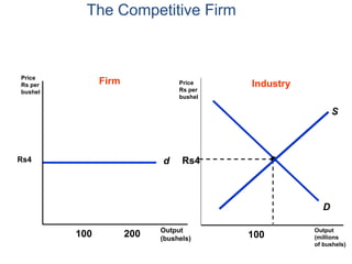
Perfectly Competitive Market:
A market structure characterized by complete ABSENCE OF RIVALRY
among the individual firms.
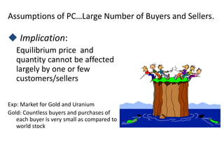
Existence of a large number of firms in Industry implying no single firm
has any power to influence the Market Price for its Product.
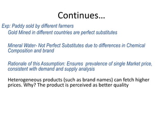
Exp: (Closest): Stock Market, Agriculture Market, Raw materials (Copper,
Iron, Cotton, Sheet Steel)
Stock Market: Face value of share is fixed
Large number of sellers and buyers in the market
Product (Share) is homogenous
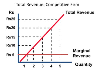
Mobilise REVENUE by selling more…..
No Asymmetry of INFORMATION
Caution: Stock prices can be sometimes becomes grossly OVERVALUED/UNDER VALUED (BULL/
BEAR Market)]
No simple indicator to judge whether a market is highly competitive or not.](https://image.slidesharecdn.com/perfectcompetition-160418161134/85/Perfect-Competition-Lecture-Notes-Economics-2-320.jpg)
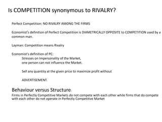
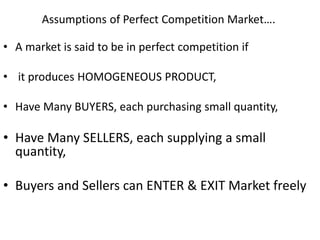
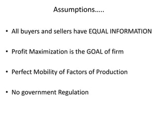
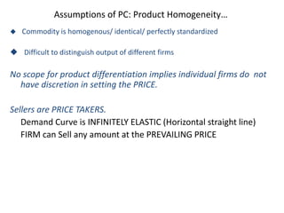
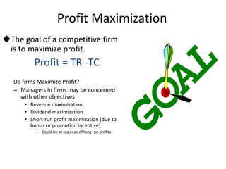
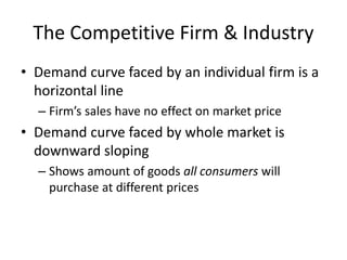


Perfect competition is a market structure with many firms and no single firm able to influence market prices. Characteristics include product homogeneity, free entry and exit of firms, equal information among buyers and sellers, and profit maximization as the primary goal. This framework serves as a benchmark for analyzing other market forms, such as monopolies and oligopolies, and understanding economic inefficiencies resulting from deviations from perfect competition.