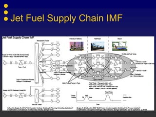
The document describes a jet fuel supply chain optimization problem modeled using IMPRESS, an industrial modeling and presolving system developed by Industrial Algorithms LLC. Key aspects include: - The supply chain involves an oil refinery, rail transport, and an airport with complex logistical constraints around product blending, cargo loading, and demand variability. - IMPRESS uses a "phenomenological decomposition" approach to decompose the mixed-integer nonlinear problem into separate logistics and quality subproblems. - Several scenarios are explored including demand variability, tank availability changes, and train reliability issues. - The base case involves over 2,000 variables, 3,000 constraints, and takes 27 seconds to solve. Scenario

1. Jet Fuel Supply Chain Design
using IMPRESS
Industrial Algorithms LLC.
Jeff Kelly & Alkis Vazacopoulos
March 24 2013
3/23/2013
Copyright, Industrial Algorithms LLC

2. Agenda
• IAL Introduction.
• What is IMPRESS?
• Jet Fuel Supply Chain & Why is it
Complex?
• Scenario Generation.
2

3. Our Mission Statement
• To provide advanced modeling and solving
tools for developing industrial applications in
the decision-making and data-mining areas.
• Our targets are:
– Operating companies in the process industries.
– Consulting service providers.
– Application software providers.

4. Our Focus
• IAL develops and markets IMPRESS, the
world’s leading software product for flowsheet
optimization in both off and on-line
environments.
• IAL provides in-house training for customers
along with complete software support and
consulting.
• IAL provides Industrial Modeling Frameworks
(IMF’s) for several problem types.
4

5. Our Industrial Modeling
Frameworks (IMF’s)
• Process industry business problems are
complex hence an IMF provides a pre-
project or pre-problem advantage.
• An IMF embeds intellectual-property
related to the process’s flowsheet
modeling as well as its problem-solving
methodology.

6. Our Modeling Environment
IMPRESS
• IMPRESS stands for “Industrial Modeling & PRE-
Solving System” and is our proprietary platform.
• You can “interface”, “interact”, “model” and
“solve” any production-chain, supply-chain,
demand-chain and/or value-chain optimization
problem.
• IMPRESS so far has been applied to:
– Production Planning
– Process Scheduling
– Pipeline & Marine Shipping
– Energy Management
6

7. Academic Collaboration &
Partnership
• Carnegie Mellon University
• University of Wisconsin
• Stevens Institute of Technology
• Fairleigh Dickinson University
• George Washington University

8. Why are we unique?
• IMPRESS is flowsheet-based (i.e., a
figurative language).
– This means that the modeling is inherently
network or superstructure “aware” with
equipment-to-equipment, resource-to-
resource, activity-to-activity, etc. as explicit
language constructs or objects.

9. Why are we unique?
• It also means that all the effort of generating
the sparse A matrix in the LP, QP, MILP and
NLP is done automatically by automating the
generation of sets, lists, parameters,
variables, constraints & derivatives when
the model is configured using our
proprietary and comprehensive library of
sub-models.
9

10. Why are we unique?
• IMPRESS is “shape/sheet-based” which
is different from other modeling systems:
– Algebraic modeling languages like GAMS,
AIMMS, AMPL, etc. are “set-based”.
– Applied engineering modeling languages like
ACM, gPROMS, APMonitor, NOVA-MS,
Modelica, etc. are “structure-based”.
– Array manipulation modeling languages like
Matlab, Mathematica, Octave, etc. are
“scalar-based”.
10

11. How do we model the flowsheet?
 Configure versus Code:
 Draw the flowsheet of connected UOPS shapes or objects
and the sets, lists, parameters, variables, constraints,
derivatives & expressions are automatically created.
 User, custom or ad hoc sub-models can also be configured
or coded when required using foreign LP files as well as
formulas and function blocks. QLQ Parameters
charge, batch & lot-sizing,
Port-State 2 input-output yields,
stream flow bounding,
min/max run-lengths & cycle-times,
sequence-dependent setups,
Port-State 1 certification delays,
density, composition & property limits,
nonlinear & discontinuous formulas,
economic, environmental & efficiency
objectives, etc.
Unit- Unit-
Operation 1 Operation 2

12. How do we configure problems?
• Problems are configured using “sheets” for
each “shape” either by:
– Interfacing with our flat-file Industrial Modeling
Language (IML) or
– Interactively with our Industrial Programming
Language (IPL) using a computer programming
language such as C, C++, C#, Java, Python, etc.

13. What is our system architecture?
• IMPRESS has six system components
called SIIMPLE:
– Server, Interfacer (IML), Interacter (IPL),
Modeler, Presolver DLL’s and an
Executable (coded in most computer
programming language) .
– Interfacer, Interacter and Modeler are
domain-specific whereas the Server,
Presolver and Executable are not i.e., they
are domain-inspecific or generic for any type
of optimization problem.

14. Jet Fuel Supply Chain IMF

15. Oil-Refinery Site
• Three crude-oils of equal compositions.
• A CDU (fractionator) with 8 compounds
(macro-cuts) with a charge of 20 Km3/day
+/- 5% and 2 swing-cuts with 2 blenders.
• A VDU (fractionator) with 3 compounds and
a possible import of reduced crude-oil.
• Jet Fuels A and B are blended with sulfur
specifications of 0.125 & 0.250 wt%.
• Two dedicated tanks for Jet Fuel A and B of
15
size 16 Km3 each.

16. Rail-Road Site
• Two “unit” trains with 100 tankers holding
120 m3 each (12 Km3 ~ 72,000 Barrels).
• Train1 can haul either Jet A or B but not
both with travel times of 4-days for both
trains.
• Train2 can haul both Jet A and B in equal
amounts.
• Partial loading of trains is allowed (> 90%).
• Only one train can load/unload at a time. 16

17. Airport Site
• Two dedicated tanks for Jet A and B of
size 14 Km3 each with an unused swing
(multi-product) tank.
• Demand for Jet A is 3.0 +/- 5% Km3/day
and for Jet B is 2.5 +/- 5% Km3/day.
17

18. Why is this problem complex?
• This is an MINLP problem involving quantity,
logic & quality phenomenological variables &
constraints i.e.,
– Closed-shop lot-sizing or inventory management
especially cargo-sizing of trains.
– Round-trip travel time of trains.
– Pooling with swing-cut blending of density and
sulfur properties (both volume and mass
blending).
18

19. How do we solve the problem?
• We perform a “phenomenological
decomposition” or “polylithic” modeling:
– Solve a MILP logistics sub-problem
(quantity*logic) in succession with a NLP
quality sub-problem (quantity*quality).
– Logic variables are fixed in the NLP and
quality variables are proxyed using fixed
yields (transfer-coefficients, intensities,
recipes, etc.) in the MILP.
19

20. What 3rd party solvers do we use?
• For MILP we have bindings to:
– COINMP, GLPK, LPSOLVE, SCIP, CPLEX,
GUROBI & XPRESS.
• For NLP we have bindings to:
– CONOPT, IPOPT, KNITRO, XPRESS-SLP as
well as our “home-grown” SLPQPE.
– SLPQPE can use all previously mentioned LP’s
as its sub-solver. If the objective function has
quadratic terms then a QP is called at each
major iteration (for nonlinear control problems).
20

21. How do we manage the data?
• All lower, upper (hard) and target (soft)
bounds are time-varying (temporal) for all
quantity, logic & quality variables.
– Data are entered in continuous-time or event-
based and digitized into time-periods.
– Data for over-lapping time-periods are
accumulated i.e., added or summed together.
– Data are provided for both past/present and
future time-horizons (allowing us to perform
data reconciliation and parameter estimation
using the same model with different data). 21

22. How do we model the data?
• All data are contained in “frames” (sheets)
with a header & trailer “feature” and multiple
feeder features with multiple “fields”.
• For dynamic data such as orders,
transactions, events, commands, etc. we
have the following format:
&sUnit,&sOperation,&sPort,&sState,@rQLQP_Lower,@rQLQP_Upper,@rQLQP_Target,@rBegin_Time,@rEnd_Time
UnitName,OperationName,PortName,StateName, lower bound , upper bound , target , begin-time , end-time
…
&sUnit,&sOperation,&sPort,&sState,@rQLQP_Lower,@rQLQP_Upper,@rQLQP_Target,@rBegin_Time,@rEnd_Time
Note: The symbol & indicates an address or key and @ indicates an attribute or value. In
addition, all number fields (‘i’ or ‘r’ prefix) can be entered as a mathematical expression. 22

23. Scenario Generation
• We explore three types of ad hoc scenarios:
– Demand Variability
– Tank Availability
– Train Reliability
• One “base-case” IML file required with 3
“delta-case” incremental IML files for each
scenario which “over-loads” the parameters.
• Goal of each delta-case scenario is to
maintain “global feasibility” of logistics
sub-problem given disturbance/disruption. 23

24. Base-Case IML File
24

25. Base-Case Yields (from NLP)
• A quality sub-problem was run as a
nonlinear planning problem with one time-
period respecting the jet fuel sulfur bounds
with fixed crude-oil composition.
– Yields computed by the quality sub-problem and
fixed in the logistics sub-problem are:
&sUnit,&sOperation,&sPort,&sState,@rYield_Lower,@rYield_Upper,@rYield_Target,@rBegin_Time,@rEnd_Time
CDU,FUELS,ATR,, 0.4511653090E+000 ,0.4511653090E+000,,BEGIN,END
CDU,FUELS,C1C2,, 0.1863222333E-002 ,0.1863222333E-002,,BEGIN,END
CDU,FUELS,C3C4,, 0.9754549000E-002 ,0.9754549000E-002,,BEGIN,END
CDU,FUELS,D,, 0.2477161380E+000 ,0.2477161380E+000,,BEGIN,END
CDU,FUELS,JDSWC,, 0.7863132167E-001,0.7863132167E-001,,BEGIN,END
CDU,FUELS,JETFUEL,, 0.1219626240E+000 ,0.1219626240E+000,,BEGIN,END
CDU,FUELS,N,, 0.5201427922E-001 ,0.5201427922E-001,,BEGIN,END
CDU,FUELS,NJSWC,, 0.3689255833E-001,0.3689255833E-001,,BEGIN,END
VDU,FUELS,HVGO,, 0.1213959870E+000 ,0.1213959870E+000,,BEGIN,END
VDU,FUELS,LVGO,, 0.5672360119E+000 ,0.5672360119E+000,,BEGIN,END
VDU,FUELS,VR,, 0.3113679995E+000 ,0.3113679995E+000,,BEGIN,END
BLENDJETA,,IN,, 0.2703321691E+000 ,0.2703321691E+000,,BEGIN,END
BLENDJETA,,IN2,, 0.7296678309E+000 ,0.7296678309E+000,,BEGIN,END
BLENDJETB,,IN,, 0.2215899306E+000 ,0.2215899306E+000,,BEGIN,END 25
BLENDJETB,,IN2,, 0.7784100694E+000 ,0.7784100694E+000,,BEGIN,END
&sUnit,&sOperation,&sPort,&sState,@rYield_Lower,@rYield_Upper,@rYield_Target,@rBegin_Time,@rEnd_Time

26. Base-Case Statistics
• Using thirty 1-day time-periods, the MILP
has circa 2225 variables, 3100 constraints,
10500 non-zeros and 750 binaries
• The objective function is $169.2 by
arbitrarily maximizing the demand flow of
Jet A and B equally i.e., prices = $1 per
Km3.
• Using SCIP as the MILP solver, this takes
27-seconds.
26

27. Base-Case Results
• A section of the Gantt chart related to the
tanks and trains is displayed below:
Superimposed Trend Lines of Holdup or Inventory
27

28. Demand Variability Scenario
• It has been observed that weekend
demand of Jet A and B is approximately
10% higher than during the week.
• Delta-case IML file contains the following:
&sUnit,&sOperation,&sPort,&sState,@rTotalRate_Lower,@rTotalRate_Upper,@rTotalRate_Target,@rBegin_Time,@rEnd_Time
JETADEMAND,,IN,,JETALOWER*WEEKEND,JETAUPPER*WEEKEND,,0,2
,,,,JETALOWER,JETAUPPER,,2,7
,,,,JETALOWER*WEEKEND,JETAUPPER*WEEKEND,,7,9
&sCalc,@sValue ,,,,JETALOWER,JETAUPPER,,9,14
WEEKEND,1.10 ,,,,JETALOWER*WEEKEND,JETAUPPER*WEEKEND,,14,16 Note: Days 1 & 2 are weekend days
JETALOWER,3-0.05*3 ,,,,JETALOWER,JETAUPPER,,16,21
JETAUPPER,3+0.05*3 and days 3 to 7 are week days etc.
,,,,JETALOWER*WEEKEND,JETAUPPER*WEEKEND,,21,23
JETBLOWER,2.5-0.05*2.5 ,,,,JETALOWER,JETAUPPER,,23,28
JETBUPPER,2.5+0.05*2.5 ,,,,JETALOWER*WEEKEND,JETAUPPER*WEEKEND,,28,30
&sCalc,@sValue JETBDEMAND,,IN,,JETBLOWER*WEEKEND,JETBUPPER*WEEKEND,,0,2
,,,,JETBLOWER,JETBUPPER,,2,7
,,,,JETBLOWER*WEEKEND,JETBUPPER*WEEKEND,,7,9
,,,,JETBLOWER,JETBUPPER,,9,14
,,,,JETBLOWER*WEEKEND,JETBUPPER*WEEKEND,,14,16
,,,,JETBLOWER,JETBUPPER,,16,21
,,,,JETBLOWER*WEEKEND,JETBUPPER*WEEKEND,,21,23
,,,,JETBLOWER,JETBUPPER,,23,28
,,,,JETBLOWER*WEEKEND,JETBUPPER*WEEKEND,,28,30 28
&sUnit,&sOperation,&sPort,&sState,@rTotalRate_Lower,@rTotalRate_Upper,@rTotalRate_Target,@rBegin_Time,@rEnd_Time

29. Demand Variability Scenario
• The objective function is $170.3 and SCIP
finds this solution in 2-seconds.
29

30. Tank Availability Scenario
• Jet B demand is lower than Jet A and the
refinery has a smaller 12 Km3 tank that it
would like to swap with the 16 Km3 Jet B
tank and use it for gasoline production.
• Delta-case IML file contains the following:
&sUnit,&sOperation,@rHoldup_Lower,@rHoldup_Upper
TANKJETA,,0,16
TANKJETAB,JETA,0,0 &sUnit,&sOperation,@rSetup_Lower,@rSetup_Upper,@rBegin_Time,@rEnd_Time
TANKJETAB,JETB,0,0 TANKJETAB,JETB,1,0,BEGIN,END
TANKJETB,,0,12 &sUnit,&sOperation,@rSetup_Lower,@rSetup_Upper,@rBegin_Time,@rEnd_Time
&sUnit,&sOperation,@rHoldup_Lower,@rHoldup_Upper
30

31. Tank Availability Scenario
• The objective function is $169.2 and SCIP
finds this solution in 18-seconds.
TANKJETAB,JETB has 0 holdup
31

32. Train Reliability Scenario
• The trains may require preventative and/or
reactive maintenance during the month.
Arbitrarily, we choose the middle and end
of the month for Train1 and Train2 down-
times of 1-days respectively.
• Delta-case IML file contains the following:
&sUnit,&sOperation,@rSetup_Lower,@rSetup_Upper,@rBegin_Time,@rEnd_Time
TRAIN1,JETA,0,-1,14,15
TRAIN1,JETB,0,-1,14,15
TRAIN2,JETAB,0,-1,29,30
&sUnit,&sOperation,@rSetup_Lower,@rSetup_Upper,@rBegin_Time,@rEnd_Time
Note: In the base-case the lower and upper logic bounds were set to 0 and 1. Therefore, to specify 0 and 0 we need to add
-1 to the upper bound. Recall that all over-lapping time-periods or intervals are cumulative.
32

33. Train Reliability Scenario
• The objective function is $168.2 and SCIP
finds this solution in 15-seconds.
Down-Time
Down-Time
33

34. How do we compare solutions
of multiple scenarios?
• By defining aggregations or key-performance
indicators (KPI’s) and computing them in a
computer programming language (Python).
• By displaying multiple solutions in the same
Gantt chart, trend plot, etc. i.e., OLAP, IBM’s
ILOG ODM or FICO’s Xpress-Insights.
• By data-mining the solutions using
compressing & clustering techniques such
as PCA, PLS, K-Means Centering, FCMC,
etc. 34

35. For a demonstration of our IMFs
35
& IMPRESS, please Contact
• Alkis Vazacopoulos
• Industrial Algorithms LLC
• Mobile: 201-256-7323
• alkis@industrialgorithms.com
Copyright, Industrial Algorithms LLC 3/23/2013

36. Questions
• Thank You!
36