Pattern baysin

Bayesian Decision Theory
Selim Aksoy
Department of Computer Engineering
Bilkent University
saksoy@cs.bilkent.edu.tr
CS 551, Fall 2018
CS 551, Fall 2018 c 2017, Selim Aksoy (Bilkent University) 1 / 46

Bayesian Decision Theory is a fundamental statistical
approach that quantiﬁes the tradeoffs between various
decisions using probabilities and costs that accompany
such decisions.
First, we will assume that all probabilities are known.
Then, we will study the cases where the probabilistic
structure is not completely known.

Fish Sorting Example Revisited
State of nature is a random variable.
Define w as the type of fish we observe (state of nature,
class) where
w = w1 for sea bass,
w = w2 for salmon.
P(w1) is the a priori probability that the next fish is a sea
bass.
P(w2) is the a priori probability that the next fish is a salmon.

Prior Probabilities
Prior probabilities reflect our knowledge of how likely each
type of fish will appear before we actually see it.
How can we choose P(w1) and P(w2)?
Set P(w1) = P(w2) if they are equiprobable (uniform priors).
May use different values depending on the fishing area, time
of the year, etc.
Assume there are no other types of fish
P(w1) + P(w2) = 1
(exclusivity and exhaustivity).

Making a Decision
How can we make a decision with only the prior
information?
Decide



w1 if P(w1) > P(w2)
w2 otherwise
What is the probability of error for this decision?
P(error) = min{P(w1), P(w2)}

Class-Conditional Probabilities
Let’s try to improve the decision using the lightness
measurement x.
Let x be a continuous random variable.
Deﬁne p(x|wj) as the class-conditional probability density
(probability of x given that the state of nature is wj for
j = 1, 2).
p(x|w1) and p(x|w2) describe the difference in lightness
between populations of sea bass and salmon.

Class-Conditional Probabilities
Figure 1: Hypothetical class-conditional probability density functions for two
classes.

Posterior Probabilities
Suppose we know P(wj) and p(x|wj) for j = 1, 2, and
measure the lightness of a ﬁsh as the value x.
Deﬁne P(wj|x) as the a posteriori probability (probability of
the state of nature being wj given the measurement of
feature value x).
We can use the Bayes formula to convert the prior
probability to the posterior probability
P(wj|x) =
p(x|wj)P(wj)
p(x)
where p(x) = 2
j=1 p(x|wj)P(wj).

Making a Decision
p(x|wj) is called the likelihood and p(x) is called the
evidence.
How can we make a decision after observing the value of x?
Decide



w1 if P(w1|x) > P(w2|x)
w2 otherwise
Rewriting the rule gives
Decide



w1 if p(x|w1)
p(x|w2)
> P(w2)
P(w1)
w2 otherwise
Note that, at every x, P(w1|x) + P(w2|x) = 1.

Probability of Error
What is the probability of error for this decision?
P(error|x) =



P(w1|x) if we decide w2
P(w2|x) if we decide w1
What is the average probability of error?
P(error) =
∞
−∞
p(error, x) dx =
∞
−∞
P(error|x) p(x) dx
Bayes decision rule minimizes this error because
P(error|x) = min{P(w1|x), P(w2|x)}.

How can we generalize to
more than one feature?
replace the scalar x by the feature vector x
more than two states of nature?
just a difference in notation
allowing actions other than just decisions?
allow the possibility of rejection
different risks in the decision?
deﬁne how costly each action is

Let {w1, . . . , wc} be the ﬁnite set of c states of nature
(classes, categories).
Let {α1, . . . , αa} be the ﬁnite set of a possible actions.
Let λ(αi|wj) be the loss incurred for taking action αi when
the state of nature is wj.
Let x be the d-component vector-valued random variable
called the feature vector.

p(x|wj) is the class-conditional probability density function.
P(wj) is the prior probability that nature is in state wj.
The posterior probability can be computed as
P(wj|x) =
p(x|wj)P(wj)
p(x)
where p(x) = c
j=1 p(x|wj)P(wj).

Conditional Risk
Suppose we observe x and take action αi.
If the true state of nature is wj, we incur the loss λ(αi|wj).
The expected loss with taking action αi is
R(αi|x) =
c
j=1
λ(αi|wj)P(wj|x)
which is also called the conditional risk.

Minimum-Risk Classiﬁcation
The general decision rule α(x) tells us which action to take
for observation x.
We want to ﬁnd the decision rule that minimizes the overall
risk
R = R(α(x)|x) p(x) dx.
Bayes decision rule minimizes the overall risk by selecting
the action αi for which R(αi|x) is minimum.
The resulting minimum overall risk is called the Bayes risk
and is the best performance that can be achieved.

Two-Category Classiﬁcation
The minimum-risk decision rule becomes
Decide



w1 if (λ21 − λ11)P(w1|x) > (λ12 − λ22)P(w2|x)
w2 otherwise
This corresponds to deciding w1 if
p(x|w1)
p(x|w2)
>
(λ12 − λ22)
(λ21 − λ11)
P(w2)
P(w1)
⇒ comparing the likelihood ratio to a threshold that is
independent of the observation x.

Minimum-Error-Rate Classiﬁcation
Actions are decisions on classes (αi is deciding wi).
If action αi is taken and the true state of nature is wj, then
the decision is correct if i = j and in error if i = j.
We want to ﬁnd a decision rule that minimizes the
probability of error.

Minimizing the risk requires maximizing P(wi|x) and results
in the minimum-error decision rule
Decide wi if P(wi|x) > P(wj|x) ∀j = i.
The resulting error is called the Bayes error and is the best
performance that can be achieved.

Figure 2: The likelihood ratio p(x|w1)/p(x|w2). The threshold θa is computed
using the priors P(w1) = 2/3 and P(w2) = 1/3, and a zero-one loss function.
If we penalize mistakes in classifying w2 patterns as w1 more than the
converse, we should increase the threshold to θb.

Discriminant Functions
A useful way of representing classifiers is through
discriminant functions gi(x), i = 1, . . . , c, where the classifier
assigns a feature vector x to class wi if
gi(x) > gj(x) ∀j = i.
For the classifier that minimizes conditional risk
gi(x) = −R(αi|x).
For the classifier that minimizes error
gi(x) = P(wi|x).

Discriminant Functions
These functions divide the feature space into c decision
regions (R1, . . . , Rc), separated by decision boundaries.
Note that the results do not change even if we replace every
gi(x) by f(gi(x)) where f(·) is a monotonically increasing
function (e.g., logarithm).
This may lead to signiﬁcant analytical and computational
simpliﬁcations.

The Gaussian Density
Gaussian can be considered as a model where the feature
vectors for a given class are continuous-valued, randomly
corrupted versions of a single typical or prototype vector.
Some properties of the Gaussian:
Analytically tractable.
Completely speciﬁed by the 1st and 2nd moments.
Has the maximum entropy of all distributions with a given
mean and variance.
Many processes are asymptotically Gaussian (Central Limit
Theorem).
Linear transformations of a Gaussian are also Gaussian.
Uncorrelatedness implies independence.

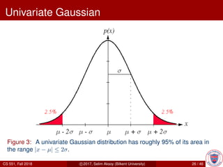
Univariate Gaussian
For x ∈ R:
p(x) = N(µ, σ2
)
=
1
√
2πσ
exp −
1
2
x − µ
σ
2
where
µ = E[x] =
∞
−∞
x p(x) dx,
σ2
= E[(x − µ)2
] =
∞
−∞
(x − µ)2
p(x) dx.

Univariate Gaussian
Figure 3: A univariate Gaussian distribution has roughly 95% of its area in
the range |x − µ| ≤ 2σ.

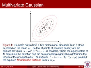
Multivariate Gaussian
For x ∈ Rd
:
p(x) = N(µ, Σ)
=
1
(2π)d/2|Σ|1/2
exp −
1
2
(x − µ)T
Σ−1
(x − µ)
where
µ = E[x] = x p(x) dx,
Σ = E[(x − µ)(x − µ)T
] = (x − µ)(x − µ)T
p(x) dx.

Multivariate Gaussian
Figure 4: Samples drawn from a two-dimensional Gaussian lie in a cloud
centered on the mean µ. The loci of points of constant density are the
ellipses for which (x − µ)T
Σ−1
(x − µ) is constant, where the eigenvectors of
Σ determine the direction and the corresponding eigenvalues determine the
length of the principal axes. The quantity r2
= (x − µ)T
Σ−1
(x − µ) is called
the squared Mahalanobis distance from x to µ.

Linear Transformations
Recall that, given x ∈ Rd
, A ∈ Rd×k
, y = AT
x ∈ Rk
,
if x ∼ N(µ, Σ), then y ∼ N(AT
µ, AT
ΣA).
As a special case, the whitening transform
Aw = ΦΛ−1/2
where
Φ is the matrix whose columns are the orthonormal
eigenvectors of Σ,
Λ is the diagonal matrix of the corresponding eigenvalues,
gives a covariance matrix equal to the identity matrix I.

Discriminant Functions for the Gaussian
Density
Discriminant functions for minimum-error-rate classiﬁcation
can be written as
gi(x) = ln p(x|wi) + ln P(wi).
For p(x|wi) = N(µi, Σi)
gi(x)=−
1
2
(x−µi)T
Σ−1
i (x−µi)−
d
2
ln2π −
1
2
ln|Σi|+lnP(wi).

Case 1: Σi = σ2
I
Discriminant functions are
gi(x) = wT
i x + wi0 (linear discriminant)
where
wi =
1
σ2
µi
wi0 = −
1
2σ2
µT
i µi + ln P(wi)
(wi0 is the threshold or bias for the i’th category).

Case 1: Σi = σ2
I
Decision boundaries are the hyperplanes gi(x) = gj(x), and
can be written as
wT
(x − x0) = 0
where
w = µi − µj
x0 =
1
2
(µi + µj) −
σ2
µi − µj
2
ln
P(wi)
P(wj)
(µi − µj).
Hyperplane separating Ri and Rj passes through the point
x0 and is orthogonal to the vector w.

Case 1: Σi = σ2
I
Figure 5: If the covariance matrices of two distributions are equal and
proportional to the identity matrix, then the distributions are spherical in d
dimensions, and the boundary is a generalized hyperplane of d − 1
dimensions, perpendicular to the line separating the means. The decision
boundary shifts as the priors are changed.

Case 1: Σi = σ2
I
Special case when P(wi) are the same for i = 1, . . . , c is the
minimum-distance classiﬁer that uses the decision rule
assign x to wi∗ where i∗
= arg min
i=1,...,c
x − µi .

Case 2: Σi = Σ
gi(x) = wT
i x + wi0 (linear discriminant)
where
wi = Σ−1
µi
wi0 = −
1
2
µT
i Σ−1
µi + ln P(wi).

Case 2: Σi = Σ
Decision boundaries can be written as
wT
(x − x0) = 0
where
w = Σ−1
(µi − µj)
x0 =
1
2
(µi + µj) −
ln(P(wi)/P(wj))
(µi − µj)T Σ−1
(µi − µj)
(µi − µj).
Hyperplane passes through x0 but is not necessarily
orthogonal to the line between the means.

Case 2: Σi = Σ
Figure 6: Probability densities with equal but asymmetric Gaussian
distributions. The decision hyperplanes are not necessarily perpendicular to
the line connecting the means.

Case 3: Σi = arbitrary
gi(x) = xT
Wix + wT
i x + wi0 (quadratic discriminant)
where
Wi = −
1
2
Σ−1
i
wi = Σ−1
i µi
wi0 = −
1
2
µT
i Σ−1
i µi −
1
2
ln |Σi| + ln P(wi).
Decision boundaries are hyperquadrics.

Figure 7: Arbitrary Gaussian distributions lead to Bayes decision boundaries
that are general hyperquadrics.

Figure 8: Arbitrary Gaussian distributions lead to Bayes decision boundaries
that are general hyperquadrics.

Error Probabilities and Integrals
For the two-category case
P(error) = P(x ∈ R2, w1) + P(x ∈ R1, w2)
= P(x ∈ R2|w1)P(w1) + P(x ∈ R1|w2)P(w2)
=
R2
p(x|w1) P(w1) dx +
R1
p(x|w2) P(w2) dx.

For the multicategory case
P(error) = 1 − P(correct)
= 1 −
c
i=1
P(x ∈ Ri, wi)
= 1 −
c
i=1
P(x ∈ Ri|wi)P(wi)
= 1 −
c
i=1 Ri
p(x|wi) P(wi) dx.

Figure 9: Components of the probability of error for equal priors and the
non-optimal decision point x∗
. The optimal point xB minimizes the total
shaded area and gives the Bayes error rate.

Receiver Operating Characteristics
Consider the two-category case and deﬁne
w1: target is present,
w2: target is not present.
Table 1: Confusion matrix.
Assigned
w1 w2
True
w1 correct detection mis-detection
w2 false alarm correct rejection
Mis-detection is also called false negative or Type II error.
False alarm is also called false positive or Type I error.

Receiver Operating Characteristics
If we use a parameter (e.g.,
a threshold) in our
decision, the plot of these
rates for different values of
the parameter is called the
receiver operating
characteristic (ROC) curve.
Figure 10: Example receiver
operating characteristic (ROC) curves
for different settings of the system.

Summary
To minimize the overall risk, choose the action that
minimizes the conditional risk R(α|x).
To minimize the probability of error, choose the class that
maximizes the posterior probability P(wj|x).
If there are different penalties for misclassifying patterns
from different classes, the posteriors must be weighted
according to such penalties before taking action.
Do not forget that these decisions are the optimal ones
under the assumption that the “true” values of the
probabilities are known.

Pattern baysin

More Related Content

What's hot

Similar to Pattern baysin

Recently uploaded

Pattern baysin