Core Concepts of Operating Systems: Processes and Scheduling

1. UNIT II - PROCESS SCHEDULING
Processes- Process Concept, Process Scheduling, Operations on Processes,
Inter process Communication; CPU Scheduling algorithms; OS – examples

2. Objectives
🠶 A process (job) is a program in execution.
🠶 The main objective of the process management module of operating system is to
manage the process submission to the system in a manner to minimize the idle time
of various processors (CPU, I/O processors e.t.c) of the computer system.
🠶 To understand the creation and deletion of processes, scheduling of various system
resources to different processes requesting them.
🠶 To describe the various mechanisms for synchronization and communication
among processes using shared memory and message passing
🠶 To introduce CPU scheduling, which is the basis for multiprogrammed operating
systems
🠶 To describe various CPU-scheduling algorithms and examine the scheduling
algorithms of several operating systems

3. What is a Process ?
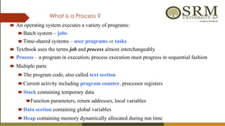
🠶 An operating system executes a variety of programs:
🠶Batch system – jobs
🠶Time-shared systems – user programs or tasks
🠶 Textbook uses the terms job and process almost interchangeably
🠶 Process – a program in execution; process execution must progress in sequential fashion
🠶 Multiple parts
🠶The program code, also called text section
🠶Current activity including program counter, processor registers
🠶Stack containing temporary data
🠶Function parameters, return addresses, local variables
🠶Data section containing global variables
🠶Heap containing memory dynamically allocated during run time

4. 🠶 Program is passive entity stored on disk, process is
active
🠶Program becomes process when executable file
loaded into memory
🠶 Execution of program started via GUI mouse clicks,
command line entry of its name, etc.
🠶 One program several processes
🠶Consider multiple users executing the same program
Process ?

5. A process control block (PCB) is a data structure used by computer operating
systems to store all the information about a process. It is also known as a
process descriptor.
🠶 When a process is created (initialized or installed), the
operating system creates a corresponding process
control block.
🠶 Information in a process control block is updated
during the transition of process states.
🠶 When the process terminates, its PCB is returned to the
pool from which new PCBs are drawn.
🠶 Each process has a single PCB.
Identifier
Status
Priority
Program Counter
Memory pointers
Context Data
I/O status Information
Accounting Information
Process control block (PCB)

6. PCB block details
Information associated with each process
(also called task control block)
🠶 Process state (Status) – running, waiting, etc
🠶 Program counter – location of instruction to next execute
🠶 CPU registers – contents of all process-centric registers
🠶 CPU scheduling information- priorities, scheduling queue pointers
🠶 Memory-management information – memory allocated to the process
🠶 Accounting information – CPU used, clock time elapsed since start, time
limits
🠶 I/O status information – I/O devices allocated to process, list of open files

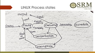
7. Process State- Five State Model
🠶 As a process executes, it changes state
🠶new: The process is being created
🠶running: Instructions are being executed
🠶waiting: The process is waiting for some event to occur
🠶ready: The process is waiting to be assigned to a processor
🠶terminated: The process has finished execution

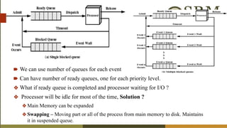
8. 🠶 We can use number of queues for each event
🠶 Can have number of ready queues, one for each priority level.
❖ What if ready queue is completed and processor waiting for I/O ?
❖ Processor will be idle for most of the time, Solution ?
❖Main Memory can be expanded
❖Swapping – Moving part or all of the process from main memory to disk. Maintains
it in suspended queue.

9. Six State Model
Suspend : Process is in secondary memory and blocked
New Ready Running
Exit
Suspend Blocked
Admit
Dispatch
Time out
Event Wait
Release
Suspend
Event Occur
Activate

10. Seven State Model
Ready / Suspend : Process is in
secondary memory is available
executing as soon as it is loaded
into main memory.
Blocked / Suspend : Process is in
secondary memory and waiting
an event.

11. Context Switching

12. 🠶 When CPU switches to another process, the system must save the state of the old
process and load the saved state for the new process.
🠶 Context-switch time is overhead; the system does no useful work while switching– an
area needing optimization.
🠶 Time dependent on hardware support.
Process Representation in Linux-
Represented by the C structure task_struct
pid t_pid; /* process identifier */
long state; /* state of the process */
unsigned int time_slice /* scheduling information */
struct task_struct *parent; /* this process’s parent */
struct list_head children; /* this process’s children */
struct files_struct *files; /* list of open files */
struct mm_struct *mm; /* address space of this process */

13. Operations on Processes - The processes can execute concurrently, and they may be created and deleted dynamically.
Process Creation
🠶 Parent process create children processes,
which, in turn create other processes,
forming a tree of processes
🠶 create-process system call
🠶 Process tree for the Solaris operating system.
The process at the top of the tree is the sched
process,with pid of 0. The sched process creates
several children processes—including pageout and
fsflush. These processes are responsible for managing
memory and file systems.
🠶 The sched process also creates the init
process, which serves as the root parent
process for all user processes.
Networking
user
login screen

14. 🠶 Resource sharing options
🠶 sub process may be able to obtain its resources directly from the operating system
🠶 Parent and children share all resources
🠶 Children share subset of parent’s resources
🠶 Parent and child share no resources
🠶 Sub process may be constrained to a subset of the resources of the parent process.
🠶 Execution options
🠶 Parent and children execute concurrently
🠶 Parent waits until children terminate
🠶 There are also two possibilities for the address space of the new process:
🠶 The child process is a duplicate of the parent process (it has the same program and data as the parent).
🠶 The child process has a new program loaded into it

15. Process Creation
🠶 Address space
🠶Child duplicate of parent
🠶Child has a program loaded into it
🠶 UNIX examples
🠶fork() system call creates new process
🠶exec() system call used after a fork() to replace
the process’ memory space with a new program

16. C Program Forking Separate Process

17. Creating a Separate Process via Windows API

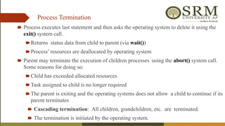
18. Process Termination
🠶 Process executes last statement and then asks the operating system to delete it using the
exit() system call.
🠶Returns status data from child to parent (via wait())
🠶Process’ resources are deallocated by operating system
🠶 Parent may terminate the execution of children processes using the abort() system call.
Some reasons for doing so:
🠶Child has exceeded allocated resources
🠶Task assigned to child is no longer required
🠶The parent is exiting and the operating systems does not allow a child to continue if its
parent terminates
🠶 Cascading termination: All children, grandchildren, etc. are terminated.
🠶 The termination is initiated by the operating system.

19. 🠶 When a process terminates, its resources are deallocated by the operating system.
However, its entry in the process table must remain there until the parent calls wait(),
because the process table contains the process’s exit status.
🠶 A process that has terminated, but whose parent has not yet called wait(), is known as
a zombie process.
🠶All processes transition to this state when they terminate, but generally they exist as zombies
only briefly. Once the parent calls wait(), the process identifier of the zombie process and its
entry in the process table are released.
🠶 What would happen if a parent did not invoke wait() and instead terminated, thereby
leaving its child processes as orphans. Linux and UNIX address this scenario by
assigning the init process as the new parent to orphan processes.
🠶 The init process periodically invokes wait()

20. Process Scheduling
🠶 Maximize CPU use, quickly switch processes onto CPU for time
sharing
🠶 Process scheduler selects among available processes for next
execution on CPU
🠶 Maintains scheduling queues of processes
🠶Job queue – set of all processes in the system
🠶Ready queue – set of all processes residing in main memory,
ready and waiting to execute
🠶Device queues – set of processes waiting for an I/O device
🠶Processes migrate among the various queues

21. Ready Queue And Various I/O Device Queues

22. Representation of Process Scheduling
● Queueing diagram represents queues, resources, flows

23. Schedulers
🠶 Short-term scheduler (or CPU scheduler) – selects one of the processes from the ready queue and
schedules them for execution
🠶 Sometimes the only scheduler in a system
🠶 Short-term scheduler is invoked frequently (milliseconds) (must be fast)
⇒
🠶 Long-term scheduler (or job scheduler) –selects processes from the storage pool in the secondary
memory and loads them into the ready queue in the main memory for execution.
🠶 Long-term scheduler is invoked infrequently (seconds, minutes) (may be slow)
⇒
🠶 The long-term scheduler controls the degree of multiprogramming (the number of processes in
memory) - If the degree of multiprogramming is stable, then the average rate of process creation must be
equal to the average departure rate of processes leaving the system.
🠶 Processes can be described as either:
🠶 I/O-bound process – spends more time doing I/O than computations, many short CPU bursts
🠶 CPU-bound process – spends more time doing computations; few very long CPU bursts
🠶 Long-term scheduler strives for good process mix

24. Medium Term Scheduling
● Medium-term scheduler can be added if degree of multiple programming needs to decrease
● Remove process from memory, store on disk, bring back in from disk to continue
execution: swapping
● Swapping is also useful to improve the mix of I/O bound and CPU bound processes in
the memory

25. CPU Scheduler
● Short-term scheduler selects from among the processes in ready queue, and allocates the CPU
to one of them
● Queue may be ordered in various ways
● CPU scheduling decisions may take place when a process:
1. Switches from running to waiting state
2. Switches from running to ready state
3. Switches from waiting to ready
4. Terminates
● Scheduling under 1 and 4 is non-preemptive
● All other scheduling is preemptive
● Consider access to shared data
● Consider preemption while in kernel mode
● Consider interrupts occurring during crucial OS activities

26. Dispatcher
🠶 Dispatcher module gives control of the CPU to the process selected by the short-term scheduler;
this involves:
🠶 switching context
🠶 switching to user mode
🠶 jumping to the proper location in the user program to restart that program
🠶 Dispatch latency – time it takes for the dispatcher to stop one process and start another running
• Under non-preemptive scheduling, once the CPU has been allocated to a process, the process
keeps the CPU until it releases the CPU either by terminating or by switching to the
waiting state.
• This scheduling method was used by Microsoft Windows 3.x. Windows 95 introduced preemptive
scheduling, and all subsequent versions of Windows operating systems have used preemptive
scheduling.
• Preemptive scheduling can result in race conditions when data are shared among several processes.

27. Scheduling Criteria
🠶 CPU utilization – keep the CPU as busy as
possible
🠶 Throughput – # of processes that complete their
execution per time unit
🠶 Turnaround time – amount of time to execute a
particular process
🠶 Waiting time – amount of time a process has been
waiting in the ready queue
🠶 Response time – amount of time it takes from
when a request was submitted until the first
response is produced, not output (for time-sharing
environment)
Scheduling Algorithm
Optimization Criteria
Max CPU utilization
Max throughput
Min turnaround time
Min waiting time
Min response time

28. First- Come, First-Served (FCFS) Scheduling
Process Burst Time
P1 24
P2 3
P3 3
🠶 Suppose that the processes arrive in the order: P1 , P2 , P3
The Gantt Chart for the schedule is:
🠶 Waiting time for P1 = 0; P2 = 24; P3 = 27
🠶 Average waiting time: (0 + 24 + 27)/3 = 17
P P P
1 2 3
0 24 30
27

29. FCFS Scheduling (Cont.)
Suppose that the processes arrive in the order:
P2 , P3 , P1
🠶 The Gantt chart for the schedule is:
🠶 Waiting time for P1 = 6; P2 = 0; P3 = 3
🠶 Average waiting time: (6 + 0 + 3)/3 = 3
🠶 Much better than previous case
🠶 Convoy effect - short process behind long process
🠶 Consider one CPU-bound and many I/O-bound processes
P1
0 3 6 30
P2
P3

30. Shortest-Job-First (SJF) Scheduling
🠶 Associate with each process the length of its next CPU burst
🠶 Use these lengths to schedule the process with the shortest time
🠶 SJF is optimal – gives minimum average waiting time for a given set of
processes
🠶The difficulty is knowing the length of the next CPU request
🠶Could ask the user
🠶 SJF scheduling is used frequently in long-term scheduling.

31. Example of SJF
ProcessArriva l Time Burst Time
P1 0.0 6
P2 2.0 8
P3 4.0 7
P4 5.0 3
🠶 SJF scheduling chart
🠶 Average waiting time = (3 + 16 + 9 + 0) / 4 = 7
P3
0 3 24
P4
P1
16
9
P2

32. Process Queue Burst time Arrival time
P1 6 2
P2 2 5
P3 8 1
P4 3 0
P5 4 4
Consider the following five processes each having its own unique burst time and arrival time.

33. Determining Length of Next CPU Burst
🠶 Can only estimate the length – should be similar to the previous one
🠶Then pick process with shortest predicted next CPU burst
🠶 Can be done by using the length of previous CPU bursts, using exponential
averaging
🠶 Commonly, α set to ½
🠶 Preemptive version called shortest-remaining-time-first

34. Prediction of the Length of the Next CPU Burst

35. Examples of Exponential Averaging
🠶 α =0
🠶τn+1 = τn
🠶Recent history does not count
🠶 α =1
🠶 τn+1 = α tn
🠶Only the actual last CPU burst counts
🠶 If we expand the formula, we get:
τn+1 = α tn+(1 - α)α tn -1 + …
+(1 - α )j
α tn -j + …
+(1 - α )n +1
τ0
🠶 Since both α and (1 - α) are less than or equal to 1, each successive term has less
weight than its predecessor

36. Example of Shortest-remaining-time-first
 Now we add the concepts of varying arrival times and preemption
to the analysis
ProcessA arri Arrival TimeT Burst Time
P1 0 8
P2 1 4
P3 2 9
P4 3 5
 Preemptive SJF Gantt Chart
 Average waiting time = [(10-1)+(1-1)+(17-2)+5-3)]/4 = 26/4 = 6.5 msec
P4
0 1 26
P1
P2
10
P3
P1
5 17

37. Priority Scheduling
🠶 A priority number (integer) is associated with each
process
🠶 The CPU is allocated to the process with the highest
priority (smallest integer ≡ highest priority)
🠶 Preemptive
🠶 Non-preemptive
🠶 SJF is priority scheduling where priority is the inverse
of predicted next CPU burst time
🠶 Problem ≡ Starvation – low priority processes may
never execute
🠶 Solution ≡ Aging – as time progresses increase the
priority of the process
• Priorities can be defined either internally or
externally.
• Internally defined priorities - time limits,
memory requirements, the number of open
files, and the ratio of average I/O burst to
average CPU burst have been used in
computing priorities.
• External priorities are set by criteria outside
the operating system, such as the importance
of the process, the type and amount of funds
being paid for computer use, the department
sponsoring the work, and other

38. Example of Priority Scheduling
Process Burst Time Priority
P1 10 3
P2 1 1
P3 2 4
P4 1 5
P5 5 2
🠶 Priority scheduling Gantt Chart
🠶 Average waiting time = 8.2 msec

39. Round Robin (RR)
🠶 Each process gets a small unit of CPU time (time quantum q), usually 10-100
milliseconds. After this time has elapsed, the process is preempted and added to the end of
the ready queue.
🠶 If there are n processes in the ready queue and the time quantum is q, then each process gets
1/n of the CPU time in chunks of at most q time units at once. No process waits more than
(n-1)q time units.
🠶 Timer interrupts every quantum to schedule next process
🠶 Performance
🠶q large FIFO
⇒
🠶q small ⇒ q must be large with respect to context switch, otherwise overhead is too high

40. Example of RR with Time Quantum = 4
Process Burst Time
P1 24
P2 3
P3 3
🠶 The Gantt chart is:
🠶 Typically, higher average turnaround than SJF, but better response
🠶 q should be large compared to context switch time
🠶 q usually 10ms to 100ms, context switch < 10 usec
P P P
1 1 1
0 18 30
26
14
4 7 10 22
P2
P3
P1
P1
P1

41. Time Quantum and Context Switch Time

42. Turnaround Time Varies With The Time Quantum
80% of CPU bursts should be
shorter than q

43. Highest Response ratio Next
• Criteria – Response Ratio
Mode – Non-Preemptive
• A Response Ratio is calculated for each of the
available jobs and the Job with the highest
response ratio is given priority over the others.
• Response Ratio = (W + S)/S
Here, W is the waiting time of the
process so far and S is the Burst time of
the process.
• Performance of HRRN –
Shorter Processes are
favoured. Aging without
service increases ratio, longer jobs
can get past shorter jobs.
Advantages
•Its performance is better than SJF Scheduling.
•It limits the waiting time of longer jobs and also supports
shorter jobs.
Disadvantages
•It can't be implemented practically.
•This is because the burst time of all the processes can not be
known in advance.

44. Multilevel Queue
🠶 Ready queue is partitioned into separate queues, eg:
🠶 foreground (interactive)
🠶 background (batch)
🠶 Process permanently in a given queue
🠶 Each queue has its own scheduling algorithm:
🠶 foreground – RR
🠶 background – FCFS
🠶 Scheduling must be done between the queues:
🠶 Fixed priority scheduling; (i.e., serve all from foreground then from background).
Possibility of starvation.
🠶 Time slice – each queue gets a certain amount of CPU time which it can
schedule amongst its processes; i.e., 80% to foreground in RR
🠶 20% to background in FCFS

45. Multilevel Queue Scheduling

46. Multilevel Feedback Queue
🠶 A process can move between the various queues; aging can be implemented
this way
🠶 Multilevel-feedback-queue scheduler defined by the following parameters:
🠶number of queues
🠶scheduling algorithms for each queue
🠶method used to determine when to upgrade a process
🠶method used to determine when to demote a process
🠶method used to determine which queue a process will enter when that
process needs service

47. Example of Multilevel Feedback Queue
🠶 Three queues:
🠶 Q0 – RR with time quantum 8 milliseconds
🠶 Q1 – RR time quantum 16 milliseconds
🠶 Q2 – FCFS
🠶 Scheduling
🠶 A new job enters queue Q0 which is served FCFS
🠶When it gains CPU, job receives 8 milliseconds
🠶If it does not finish in 8 milliseconds, job is moved to
queue Q1
🠶 At Q1 job is again served FCFS and receives 16
additional milliseconds
🠶If it still does not complete, it is preempted and

48. Multiple-Processor Scheduling
🠶 If multiple CPUs are available, load sharing becomes possible
🠶 CPU scheduling more complex when multiple CPUs are available
🠶 Homogeneous processors within a multiprocessor
🠶 Asymmetric multiprocessing – only one processor accesses the system data structures,
alleviating the need for data sharing
🠶 Symmetric multiprocessing (SMP) – each processor is self-scheduling, all processes in
common ready queue, or each has its own private queue of ready processes
🠶 Currently, most common
🠶 Processor affinity – process has affinity for processor on which it is currently running
🠶 soft affinity
🠶 hard affinity
🠶 Variations including processor sets

49. NUMA and CPU Scheduling
Note that memory-placement algorithms can also consider affinity

50. Multiple-Processor Scheduling – Load Balancing
🠶 If SMP, need to keep all CPUs loaded for efficiency
🠶 Load balancing attempts to keep workload evenly distributed
🠶 Push migration – Periodic task checks load on each processor, and if found pushes
task from overloaded CPU to other CPUs
🠶 Pull migration – idle processors pulls waiting task from busy processor
🠶 Recent trend to place multiple processor cores on same physical chip
🠶 Faster and consumes less power
🠶 Multiple threads per core also growing
🠶Takes advantage of memory stall to make progress on another thread while
memory retrieve happens
⮚ Multicore Processors

51. Multithreaded Multicore System

52. Real-Time CPU Scheduling
🠶 Can present obvious challenges
🠶 Soft real-time systems – no guarantee as to
when critical real-time process will be
scheduled
🠶 Hard real-time systems – task must be
serviced by its deadline
🠶 Two types of latencies affect performance
1. Interrupt latency – time from arrival of
interrupt to start of routine that services
interrupt
2. Dispatch latency – time for schedule to
take current process off CPU and switch
to another

53. Real-Time CPU Scheduling (Cont.)
🠶 Conflict phase of dispatch latency:
1. Preemption of any process running in
kernel mode
2. Release by low-priority process of
resources needed by high-priority
processes

54. Priority-based Scheduling
🠶 For real-time scheduling, scheduler must support preemptive, priority-based scheduling
🠶 But only guarantees soft real-time
🠶 For hard real-time must also provide ability to meet deadlines
🠶 Processes have new characteristics: periodic ones require CPU at constant intervals
🠶 Has processing time t, deadline d, period p
🠶 0 ≤ t ≤ d ≤ p
🠶 Rate of periodic task is 1/p

55. 🠶 What is unusual about this form of scheduling is that a process may have to announce its
deadline requirements to the scheduler.
🠶 admission-control algorithm- the scheduler does one of two things. It either admits the
process, guaranteeing that the process will complete on time, or rejects the request as
impossible if it cannot guarantee that the task will be serviced by its deadline.
Rate-Monotonic Scheduling
🠶 The rate-monotonic scheduling algorithm schedules periodic tasks using a static priority
policy with preemption.
🠶 Upon entering the system, each periodic task is assigned a priority inversely based on its
period.
🠶 Assumes that every time a process acquires the CPU, the duration of its CPU burst is the
same.

56. 🠶 Let’s consider an example.
P 1 and P 2 . The periods for P 1=50 and P 2 =100,
The processing times are t 1 = 20 for P 1 and t 2 = 35 for P 2 .
The deadline for each process requires that it complete its CPU burst by the start of its next
period.
Suppose we assign P 2 a higher priority than P 1.
so the scheduler has caused
P1 to miss its deadline.

57. 🠶 P1 starts first and completes its CPU burst at time 20, thereby meeting its first deadline
🠶 P2 starts running at this point and runs until time 50. At this time, it is preempted by P1 ,
although it still has 5 milliseconds remaining in its CPU burst. P1 completes its CPU burst at
time 70, at which point the scheduler resumes P2 . P2 completes its CPU burst at time 75, also
meeting its first deadline. The system is idle until time 100, when P1 is scheduled again.
P 1 and P 2 . The periods for P 1=50 and P 2 =100,
The processing times are t 1 = 20 for P 1 and t 2 = 35 for P 2 .
Rate-Monotonic Scheduling

58. Earliest-Deadline-First Scheduling
🠶 Earliest-deadline-first (EDF) scheduling dynamically assigns priorities according to deadline.
The earlier the deadline, the higher the priority; the later the deadline, the lower the priority.
🠶 when a process becomes runnable, it must announce its deadline requirements to the system
🠶 P1 has values of p1 = 50 and t1 = 25 and that
🠶 P2 has values of p2 = 80 and t2 = 35.
https://forms.gle/B2ZKyp5eHNyXEAab6

59. Interprocess Communication
🠶 Processes within a system may be independent or cooperating
🠶 Cooperating process can affect or be affected by other processes, including sharing data
🠶 Clearly, any process that shares data with other processes is a cooperating process.
🠶 Reasons for cooperating processes:
🠶 Information sharing
🠶 Computation speedup
🠶 Modularity
🠶 Convenience
🠶 Cooperating processes need Interprocess communication (IPC)
🠶 Two models of IPC
🠶 Shared memory
🠶 Message passing

60. Communications Models
(a) Message passing. (b) shared memory.
• Message passing is useful for exchanging smaller
amounts of data.
• Message passing is also easier to implement than
shared memory.
• Message-passing systems are typically implemented
using system calls and thus require the more time-
consuming task of kernel intervention.
• Shared memory allows maximum speed and
convenience of communication. System calls are
required only to establish shared-memory regions.
• Once shared memory is established, all accesses are
treated as routine memory accesses, and no assistance
from the kernel is required.

61. Shared-Memory Systems
🠶 Communicating processes to establish a region of shared memory.
🠶 Shared-memory region resides in the address space of the process.
🠶 Other processes that wish to communicate using this shared-memory segment must
attach it to their address space.
🠶 Shared memory requires that two or more processes can exchange information by
reading and writing data in the shared areas.
🠶 The processes are also responsible for ensuring that they are not writing to the same
location simultaneously.
🠶 Paradigm for cooperating processes, producer process produces information
that is consumed by a consumer process
🠶 unbounded-buffer places no practical limit on the size of the buffer
🠶 bounded-buffer assumes that there is a fixed buffer size
Producer-Consumer Problem

62. Bounded-Buffer – Shared-Memory Solution
🠶 Shared data
#define BUFFER_SIZE 10
typedef struct {
. . .
} item;
item buffer[BUFFER_SIZE];
int in = 0;
int out = 0;
🠶 Solution is correct, but can only use BUFFER_SIZE-1 elements
The producer and consumer must be synchronized,
so that the consumer does not try to consume an
item that has not yet been produced
The shared buffer is implemented as a circular array
with two logical pointers:
in and out. The variable in points to the next free
position in the buffer;
Out points to the first full position in the buffer. The
buffer is empty when in == out;
the buffer is full when ((in + 1) % BUFFER SIZE)
== out.

63. Bounded-Buffer – Producer
item next_produced;
while (true) {
/* produce an item in next produced */
while (((in + 1) % BUFFER_SIZE) ==
out)
; /* do nothing */
buffer[in] = next_produced;
in = (in + 1) % BUFFER_SIZE;
}
item next_consumed;
while (true) {
while (in == out)
; /* do nothing */
next_consumed = buffer[out];
out = (out + 1) % BUFFER_SIZE;
/* consume the item in next consumed */
}
Bounded Buffer – Consumer

64. Interprocess Communication – Message Passing
🠶 Message passing provides a mechanism to allow processes to communicate
🠶 Mechanism for processes to communicate and synchronize their actions
without sharing the same address space (useful in a distributed
environment)
🠶 Chat participants communicate with one another by exchanging messages
🠶 Message system – processes communicate with each other without
resorting to shared variables
🠶 IPC facility provides two operations:
🠶send(message)
🠶receive(message)
🠶 The message size is either fixed or variable

65. Message Passing (Cont.)
🠶 If processes P and Q wish to communicate, they need to:
🠶 Establish a communication link between them
🠶 Exchange messages via send/receive
🠶 Implementation issues:
🠶 How are links established
🠶 Can a link be associated with more than two processes?
🠶 How many links can there be between every pair of communicating
processes?
🠶 What is the capacity of a link?
🠶 Is the size of a message that the link can accommodate fixed or variable?
🠶 Is a link unidirectional or bi-directional

66. Message Passing (Cont.)
🠶 Implementation of communication link
🠶 Physical:
🠶Shared memory
🠶Hardware bus
🠶Network
🠶 Logical:
🠶 Direct or indirect
🠶 Synchronous or asynchronous
🠶 Automatic or explicit buffering

67. Direct Communication
🠶 Naming- Processes must name each other explicitly:
🠶 send (P, message) – send a message to process P
🠶 receive(Q, message) – receive a message from process Q
🠶 Properties of communication link
🠶 Links are established automatically
🠶 A link is associated with exactly one pair of communicating
processes
🠶 Between each pair there exists exactly one link
🠶 The link may be unidirectional, but is usually bi-directional

68. Indirect Communication
🠶 Messages are directed and received from mailboxes (also referred to as ports)
🠶 Each mailbox has a unique id
🠶 Processes can communicate only if they share a mailbox
🠶 Properties of communication link
🠶 Link established only if processes share a common mailbox
🠶 A link may be associated with many processes
🠶 Each pair of processes may share several communication links
🠶 Link may be unidirectional or bi-directional

69. Indirect Communication
🠶 The messages are sent to and received from mailboxes, or ports.
🠶 Operations
🠶 create a new mailbox (port)
🠶 send and receive messages through mailbox
🠶 destroy a mailbox
🠶 Primitives are defined as:
send(A, message) – send a message to mailbox A
receive(A, message) – receive a message from mailbox A
🠶 communication link has the following properties:
• A link is established between a pair of processes only if both members of the pair have
a shared mailbox.
• A link may be associated with more than two processes.
• Between each pair of communicating processes, there may be a number of different
links, with each link corresponding to one mailbox.

70. Indirect Communication
🠶 Mailbox sharing
🠶 P1, P2, and P3 share mailbox A
🠶 P1, sends; P2 and P3 receive
🠶 Who gets the message?
🠶 Solutions
🠶 Allow a link to be associated with at most two processes
🠶 Allow only one process at a time to execute a receive operation
🠶 Allow the system to select arbitrarily the receiver. Sender is notified who the
receiver was.

71. Synchronization
🠶 Message passing may be either blocking or non-blocking
🠶 Blocking is considered synchronous
🠶 Blocking send -- the sender is blocked until the message is received
🠶 Blocking receive -- the receiver is blocked until a message is available
🠶 Non-blocking is considered asynchronous
🠶 Non-blocking send -- the sender sends the message and continue
🠶 Non-blocking receive -- the receiver receives:
● A valid message, or
● Null message
● Different combinations possible
● If both send and receive are blocking, we have a rendezvous

72. Synchronization (Cont.)
Producer-consumer becomes trivial
message next_produced;
while (true) {
/* produce an item in next produced */
send(next_produced);
}
message next_consumed;
while (true) {
receive(next_consumed);
/* consume the item in next consumed */
}

73. Process Representation in Linux
Represented by the C structure task_struct
pid t_pid; /* process identifier */
long state; /* state of the process */
unsigned int time_slice /* scheduling information */
struct task_struct *parent; /* this process’s parent */
struct list_head children; /* this process’s children */
struct files_struct *files; /* list of open files */
struct mm_struct *mm; /* address space of this process */
OS Examples

74. 🠶 Usually after fork() call, the child process and the parent process would perform different tasks. If the same task
needs to be run, then for each fork() call it would run 2 power n times, where n is the number of times fork() is
invoked.
#include <stdio.h>
#include <sys/types.h>
#include <unistd.h>
int main() {
fork();
printf("Called fork() system calln");
return 0;
}

75. Examples of IPC Systems - POSIX
● POSIX Shared Memory
● Process first creates shared memory segment
shm_fd = shm_open(name, O CREAT | O RDWR, 0666);
● Also used to open an existing segment to share it
● Set the size of the object
ftruncate(shm fd, 4096);
● Now the process could write to the shared memory
sprintf(shared memory, "Writing to shared memory");

76. IPC POSIX Producer

77. IPC POSIX Consumer

78. Examples of IPC Systems – Windows
🠶 Message-passing centric via advanced local procedure call (LPC) facility
🠶 Only works between processes on the same system
🠶 Uses ports (like mailboxes) to establish and maintain communication channels
🠶 Communication works as follows:
🠶 The client opens a handle to the subsystem’s connection port object.
🠶 The client sends a connection request.
🠶 The server creates two private communication ports and returns the handle to one of
them to the client.
🠶 The client and server use the corresponding port handle to send messages or callbacks
and to listen for replies.

79. Local Procedure Calls in Windows

80. UNIX Process states
🠶 v

81. LINUX Process states
🠶

82. Solaris Scheduling
Solaris uses priority-based thread scheduling where each thread belongs to
one of six classes:
🠶 1. Time sharing (TS)
🠶 2. Interactive (IA)
🠶 3. Real time (RT)
🠶 4. System (SYS)
🠶 5. Fair share (FSS)
🠶 6. Fixed priority (FP)

83. Windows Scheduling
🠶 Windows schedules threads using a priority-based preemptive scheduling
Algorithm.
🠶 The Windows scheduler ensures that the highest-priority thread will always run.
🠶 The portion of the Windows kernel that handles scheduling is called the dispatcher.
🠶 A thread selected to run by the dispatcher will run until it is preempted by a higher-
priority thread, until it terminates, until its time quantum ends, or until it calls a
blocking system call, such as for I/O.
🠶 If a higher-priority real-time thread becomes ready while a lower-priority thread is
running, the lower-priority thread will be preempted. This preemption gives a real-time
thread preferential access to the CPU when the thread needs such access.

84. The base priorities for each priority class are:
🠶 REALTIME PRIORITY CLASS—24
🠶 HIGH PRIORITY CLASS—13
🠶 ABOVE NORMAL PRIORITY CLASS—10
🠶 NORMAL PRIORITY CLASS—8
🠶 BELOW NORMAL PRIORITY CLASS—6
🠶 IDLE PRIORITY CLASS—4

85. Linux Scheduling
🠶 provides a scheduling algorithm that runs in constant time—known as O(1)—
regardless of the number of tasks on the system.
🠶 The Linux scheduler is a preemptive, priority-based algorithm with two separate
priority ranges: a real-time range from 0 to 99 and a nice value ranging from 100 to
140.
🠶 Linux assigns higher-priority tasks longer time quanta and lower-priority tasks shorter
time quanta
🠶 The kernel maintains a list of all runnable tasks in a runqueue data structure. Each
processor maintains its own runqueue and schedules itself independently. Each
runqueue contains two priority arrays: active and expired.