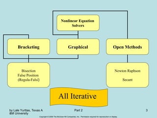
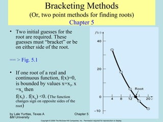
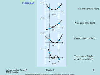
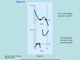
Chapter 5 discusses methods for finding roots of nonlinear equations, focusing on bracketing methods like the bisection and false-position (regula falsi) methods. It outlines the steps to implement these methods, including the necessary conditions for convergence and the evaluation of their pros and cons. The chapter emphasizes the importance of selecting appropriate initial guesses and understanding the behavior of the function to ensure accurate root approximation.

1. by Lale Yurttas, Texas A
&M University
Chapter 5 1
Copyright © 2006 The McGraw-Hill Companies, Inc. Permission required for reproduction or display.
Chapter 5

2. by Lale Yurttas, Texas A
&M University
Part 2 2
Copyright © 2006 The McGraw-Hill Companies, Inc. Permission required for reproduction or display.
Roots of Equations
Part 2
•Why?
•But
a
ac
b
b
x
c
bx
ax
2
4
0
2
2 







?
0
sin
?
0
2
3
4
5












x
x
x
x
f
ex
dx
cx
bx
ax

3. by Lale Yurttas, Texas A
&M University
Part 2 3
Copyright © 2006 The McGraw-Hill Companies, Inc. Permission required for reproduction or display.
Nonlinear Equation
Solvers
Bracketing Graphical Open Methods
Bisection
False Position
(Regula-Falsi)
Newton Raphson
Secant
All Iterative

4. by Lale Yurttas, Texas A
&M University
Chapter 5 4
Copyright © 2006 The McGraw-Hill Companies, Inc. Permission required for reproduction or display.
Bracketing Methods
(Or, two point methods for finding roots)
Chapter 5
• Two initial guesses for the
root are required. These
guesses must “bracket” or be
on either side of the root.
== > Fig. 5.1
• If one root of a real and
continuous function, f(x)=0,
is bounded by values x=xl, x
=xu then
f(xl) . f(xu) <0. (The function
changes sign on opposite sides of the
root)

5. by Lale Yurttas, Texas A
&M University
Chapter 5 5
Copyright © 2006 The McGraw-Hill Companies, Inc. Permission required for reproduction or display.
Figure 5.2
No answer (No root)
Nice case (one root)
Oops!! (two roots!!)
Three roots( Might
work for a while!!)

6. by Lale Yurttas, Texas A
&M University
Chapter 5 6
Copyright © 2006 The McGraw-Hill Companies, Inc. Permission required for reproduction or display.
Figure 5.3
Two roots( Might
work for a while!!)
Discontinuous
function. Need
special method

7. by Lale Yurttas, Texas A
&M University
Chapter 5 7
Copyright © 2006 The McGraw-Hill Companies, Inc. Permission required for reproduction or display.
Figure 5.4a
Figure 5.4b
Figure 5.4c
MANY-MANY roots. What do we
do?
f(x)=sin 10x+cos 3x

8. by Lale Yurttas, Texas A
&M University
Chapter 5 8
Copyright © 2006 The McGraw-Hill Companies, Inc. Permission required for reproduction or display.
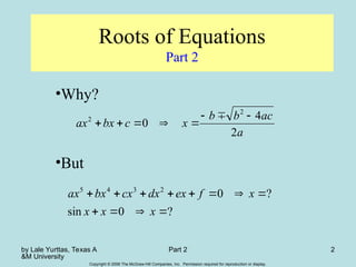
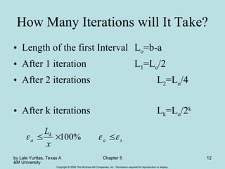
The Bisection Method
For the arbitrary equation of one variable, f(x)=0
1. Pick xl and xu such that they bound the root of
interest, check if f(xl).f(xu) <0.
2. Estimate the root by evaluating f[(xl+xu)/2].
3. Find the pair
• If f(xl). f[(xl+xu)/2]<0, root lies in the lower interval,
then xu=(xl+xu)/2 and go to step 2.

9. by Lale Yurttas, Texas A
&M University
Chapter 5 9
Copyright © 2006 The McGraw-Hill Companies, Inc. Permission required for reproduction or display.
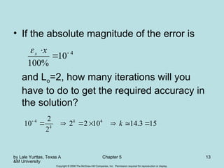
• If f(xl). f[(xl+xu)/2]>0, root
lies in the upper interval, then
xl= [(xl+xu)/2, go to step 2.
• If f(xl). f[(xl+xu)/2]=0, then
root is (xl+xu)/2 and
terminate.
4. Compare s with a
5. If a<s, stop. Otherwise
repeat the process.
%
100
2
2
%
100
2
2


u
l
u
l
u
u
l
u
l
l
x
x
x
x
x
or
x
x
x
x
x







10. by Lale Yurttas, Texas A
&M University
Chapter 5 10
Copyright © 2006 The McGraw-Hill Companies, Inc. Permission required for reproduction or display.
Figure 5.6

11. by Lale Yurttas, Texas A
&M University
Chapter 5 11
Copyright © 2006 The McGraw-Hill Companies, Inc. Permission required for reproduction or display.
Evaluation of Method
Pros
• Easy
• Always find root
• Number of iterations
required to attain an
absolute error can be
computed a priori.
Cons
• Slow
• Know a and b that
bound root
• Multiple roots
• No account is taken of
f(xl) and f(xu), if f(xl) is
closer to zero, it is likely
that root is closer to xl .

12. by Lale Yurttas, Texas A
&M University
Chapter 5 12
Copyright © 2006 The McGraw-Hill Companies, Inc. Permission required for reproduction or display.
How Many Iterations will It Take?
• Length of the first Interval Lo=b-a
• After 1 iteration L1=Lo/2
• After 2 iterations L2=Lo/4
• After k iterations Lk=Lo/2k
s
a
k
a
x
L


 

 %
100

13. by Lale Yurttas, Texas A
&M University
Chapter 5 13
Copyright © 2006 The McGraw-Hill Companies, Inc. Permission required for reproduction or display.
• If the absolute magnitude of the error is
and Lo=2, how many iterations will you
have to do to get the required accuracy in
the solution?
4
10
%
100


x
s

15
3
.
14
10
2
2
2
2
10 4
4








k
k
k

14. by Lale Yurttas, Texas A
&M University
Chapter 5 14
Copyright © 2006 The McGraw-Hill Companies, Inc. Permission required for reproduction or display.
The False-Position Method
(Regula-Falsi)
• If a real root is
bounded by xl and xu of
f(x)=0, then we can
approximate the
solution by doing a
linear interpolation
between the points [xl,
f(xl)] and [xu, f(xu)] to
find the xr value such
that l(xr)=0, l(x) is the
linear approximation
of f(x).
== > Fig. 5.12

15. by Lale Yurttas, Texas A
&M University
Chapter 5 15
Copyright © 2006 The McGraw-Hill Companies, Inc. Permission required for reproduction or display.
Procedure
1. Find a pair of values of x, xl and xu such that
fl=f(xl) <0 and fu=f(xu) >0.
2. Estimate the value of the root from the
following formula (Refer to Box 5.1)
and evaluate f(xr).
l
u
l
u
u
l
r
f
f
f
x
f
x
x




16. by Lale Yurttas, Texas A
&M University
Chapter 5 16
Copyright © 2006 The McGraw-Hill Companies, Inc. Permission required for reproduction or display.
3. Use the new point to replace one of the
original points, keeping the two points on
opposite sides of the x axis.
If f(xr)<0 then xl=xr == > fl=f(xr)
If f(xr)>0 then xu=xr == > fu=f(xr)
If f(xr)=0 then you have found the root and
need go no further!

17. by Lale Yurttas, Texas A
&M University
Chapter 5 17
Copyright © 2006 The McGraw-Hill Companies, Inc. Permission required for reproduction or display.
4. See if the new xl and xu are close enough for
convergence to be declared. If they are not go back
to step 2.
• Why this method?
– Faster
– Always converges for a single root.
See Sec.5.3.1, Pitfalls of the False-Position Method
Note: Always check by substituting estimated root in the
original equation to determine whether f(xr) ≈ 0.