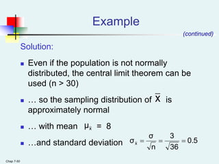
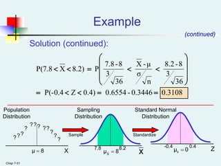
SlideShare a Scribd company logo
1 of 53
Statistics for Managers Using Microsoft Excel® 7e Copyright ©2014 Pearson Education, Inc. Chap 6-1
Sections 6.1-6.3, 7.1-7.2
Normal Distribution and
Parameter Estimation
Statistics for Managers Using Microsoft Excel® 7e Copyright ©2014 Pearson Education, Inc. Chap 6-2
Learning Objectives
In this chapter, you learn:
 How continuous distributions are different from discrete
distributions.
 How to compute probabilities from the normal
distribution
 How to use the normal distribution to solve business
problems
Statistics for Managers Using Microsoft Excel® 7e Copyright ©2014 Pearson Education, Inc. Chap 6-3
Continuous Probability Distributions
 A continuous random variable is a variable that
can assume any value on an interval
 thickness of an item, weight, length
 time required to complete a task
 temperature
 height, in inches
 miles per gallon
Probability Density
Chap 5-4
 A function f(x) ≥ 0 that shows the more likely
and less likely intervals of variable X.
 P(a ≤ X ≤ b) = area under f(x) from a to b
a b X
f(X) P a X b
( )
≤
≤
P a X b
( )
<
<
=
(Note that the
probability of any
individual value is zero)
Statistics for Managers Using Microsoft Excel® 7e Copyright ©2014 Pearson Education, Inc. Chap 5-5
Statistics for Managers Using Microsoft Excel® 7e Copyright ©2014 Pearson Education, Inc. Chap 6-5
Probability is the area under the
density curve
a b X
f(X) P a X b
( )
≤
≤
P a X b
( )
<
<
=
(Note that the
probability of any
individual value is zero)
Statistics for Managers Using Microsoft Excel® 7e Copyright ©2014 Pearson Education, Inc. Chap 6-6
The Normal Distribution
 ‘Bell Shaped’
 Symmetrical
 Mean, Median and Mode
are Equal
Location is determined by the
mean, μ
Spread is determined by the
standard deviation, σ
The random variable has an
infinite theoretical range:
+  to  
Mean
= Median
= Mode
X
f(X)
μ
σ
Statistics for Managers Using Microsoft Excel® 7e Copyright ©2014 Pearson Education, Inc. Chap 6-7
The Normal Distribution
Density Function
2
μ)
(X
2
1
e
2π
1
f(X)





 

 

 The formula for the normal probability density function is
Where e = the mathematical constant approximated by 2.71828
π = the mathematical constant approximated by 3.14159
μ = the population mean
σ = the population standard deviation
X = any value of the continuous variable
Statistics for Managers Using Microsoft Excel® 7e Copyright ©2014 Pearson Education, Inc. Chap 6-8
By varying the parameters μ and σ, we obtain
different normal distributions
Many Normal Distributions
Statistics for Managers Using Microsoft Excel® 7e Copyright ©2014 Pearson Education, Inc. Chap 6-9
The Normal Distribution
Shape
X
f(X)
μ
σ
Changing μ shifts the
distribution left or right.
Changing σ increases
or decreases the
spread.
Statistics for Managers Using Microsoft Excel® 7e Copyright ©2014 Pearson Education, Inc. Chap 6-10
The Standardized Normal
 Any normal distribution (with any mean μ and
standard deviation σ) can be transformed into
the standardized normal distribution (Z)
 The standardized normal distribution (Z) has a
mean of 0 and a standard deviation of 1
σ
μ
X
Z


Statistics for Managers Using Microsoft Excel® 7e Copyright ©2014 Pearson Education, Inc. Chap 6-11
The Standardized
Normal Distribution
 Also known as the “Z” distribution
 Mean is 0
 Standard Deviation is 1
Z
f(Z)
0
1
Values above the mean have positive Z-values,
values below the mean have negative Z-values
Statistics for Managers Using Microsoft Excel® 7e Copyright ©2014 Pearson Education, Inc. Chap 6-12
f(X)
X
μ
Probability as
Area Under the Curve
0.5
0.5
The total area under the curve is 1.0, and the curve is
symmetric, so half is above the mean, half is below
1.0
)
X
P( 




0.5
)
X
P(μ 



0.5
μ)
X
P( 



Statistics for Managers Using Microsoft Excel® 7e Copyright ©2014 Pearson Education, Inc. Chap 6-13
The Standardized Normal Table
 The Cumulative Standardized Normal table
in the textbook (Appendix table E.2) gives the
probability less than a desired value of Z (i.e.,
from negative infinity to Z)
Z
0 2.00
0.9772
Example:
P(Z < 2.00) = 0.9772
Statistics for Managers Using Microsoft Excel® 7e Copyright ©2014 Pearson Education, Inc. Chap 6-14
The Standardized Normal Table
The value within the
table gives the
probability from Z =  
up to the desired Z
value
.9772
2.0
P(Z < 2.00) = 0.9772
The row shows
the value of Z
to the first
decimal point
The column gives the value of
Z to the second decimal point
2.0
.
.
.
(continued)
Z 0.00 0.01 0.02 …
0.0
0.1
Statistics for Managers Using Microsoft Excel® 7e Copyright ©2014 Pearson Education, Inc. Chap 6-15
General Procedure for
Finding Normal Probabilities
 Draw the normal curve for the problem in
terms of X
 Standardize X by computing Z
 Use the Standardized Normal Table for Z
To find P(a < X < b) when X is
distributed normally:
Statistics for Managers Using Microsoft Excel® 7e Copyright ©2014 Pearson Education, Inc. Chap 6-16
Example
 Let X represent the time it takes (in seconds)
to download an image file from the internet.
 Suppose X is normal with a mean of 18.0
seconds and a standard deviation of 5.0
seconds. Find P(X < 18.6)
18.6
X
18.0
Statistics for Managers Using Microsoft Excel® 7e Copyright ©2014 Pearson Education, Inc. Chap 6-17
 Let X represent the time it takes, in seconds to download an image file
from the internet.
 Suppose X is normal with a mean of 18.0 seconds and a standard
deviation of 5.0 seconds. Find P(X < 18.6)
Z
0.12
0
X
18.6
18
μ = 18
σ = 5
μ = 0
σ = 1
(continued)
Finding Normal Probabilities
0.12
5.0
8.0
1
18.6
σ
μ
X
Z 




P(X < 18.6) P(Z < 0.12)
Statistics for Managers Using Microsoft Excel® 7e Copyright ©2014 Pearson Education, Inc. Chap 6-18
Z
0.12
Z .00 .01
0.0 .5000 .5040 .5080
.5398 .5438
0.2 .5793 .5832 .5871
0.3 .6179 .6217 .6255
Solution: Finding P(Z < 0.12)
0.5478
.02
0.1 .5478
Standardized Normal Probability
Table (Portion)
0.00
= P(Z < 0.12)
P(X < 18.6)
Statistics for Managers Using Microsoft Excel® 7e Copyright ©2014 Pearson Education, Inc. Chap 6-19
Finding Normal
Upper Tail Probabilities
 Suppose X is normal with mean 18.0
and standard deviation 5.0.
 Now Find P(X > 18.6)
X
18.6
18.0
Statistics for Managers Using Microsoft Excel® 7e Copyright ©2014 Pearson Education, Inc. Chap 6-20
 Now Find P(X > 18.6) by the complement rule…
(continued)
Z
0.12
0
Z
0.12
0.5478
0
1.000 1.0 - 0.5478
= 0.4522
P(X > 18.6) = P(Z > 0.12) = 1.0 - P(Z ≤ 0.12)
= 1.0 - 0.5478 = 0.4522
Finding Normal
Upper Tail Probabilities
Statistics for Managers Using Microsoft Excel® 7e Copyright ©2014 Pearson Education, Inc. Chap 6-21
 Suppose X is normal with mean 18.0
and standard deviation 5.0.
 Find P(17.4 < X < 18)
X
17.4
18.0
Probabilities in the Lower Tail
Statistics for Managers Using Microsoft Excel® 7e Copyright ©2014 Pearson Education, Inc. Chap 6-22
Probabilities in the Lower Tail
Find P(17.4 < X < 18)…
X
17.4 18.0
P(17.4 < X < 18)
= P(-0.12 < Z < 0)
= P(Z < 0) – P(Z ≤ -0.12)
= 0.5000 - 0.4522 = 0.0478
(continued)
0.0478
0.4522
Z
-0.12 0
The Normal distribution is
symmetric, so this probability
is the same as P(0 < Z < 0.12)
Statistics for Managers Using Microsoft Excel® 7e Copyright ©2014 Pearson Education, Inc. Chap 6-23
“Empirical” Rules
μ ± 1σ encloses about
68.26% of X’s
f(X)
X
μ μ+1σ
μ-1σ
What can we say about the distribution of values
around the mean? For any normal distribution:
σ
σ
68.26%
Statistics for Managers Using Microsoft Excel® 7e Copyright ©2014 Pearson Education, Inc. Chap 6-24
The Empirical Rule
 μ ± 2σ covers about 95% of X’s
 μ ± 3σ covers about 99.7% of X’s
x
μ
2σ 2σ
x
μ
3σ 3σ
95.44% 99.73%
(continued)
Example
 Page 203, #6.7(a,b,c)
#6.7d… Inverse problem… We know the
probability, but we need the value of X
Statistics for Managers Using Microsoft Excel® 7e Copyright ©2014 Pearson Education, Inc. Chap 5-25
Statistics for Managers Using Microsoft Excel® 7e Copyright ©2014 Pearson Education, Inc. Chap 6-26
 Steps to find the X value for a known
probability:
1. Find the Z value for the known probability
2. Convert to X units using the formula:
Given a Normal Probability
Find the X Value
Zσ
μ
X 

Statistics for Managers Using Microsoft Excel® 7e Copyright ©2014 Pearson Education, Inc. Chap 6-27
Finding the X value for a
Known Probability
Example:
 Let X represent the time it takes (in seconds) to
download an image file from the internet.
 Suppose X is normal with mean 18.0 and standard
deviation 5.0
 Find X such that 20% of download times are less than
X.
X
? 18.0
0.2000
Z
? 0
(continued)
Statistics for Managers Using Microsoft Excel® 7e Copyright ©2014 Pearson Education, Inc. Chap 6-28
Find the Z value for
20% in the Lower Tail
 20% area in the lower
tail is consistent with a
Z value of -0.84
Z .03
-0.9 .1762 .1736
.2033
-0.7 .2327 .2296
.04
-0.8 .2005
Standardized Normal Probability
Table (Portion)
.05
.1711
.1977
.2266
…
…
…
…
X
? 18.0
0.2000
Z
-0.84 0
1. Find the Z value for the known probability
Statistics for Managers Using Microsoft Excel® 7e Copyright ©2014 Pearson Education, Inc. Chap 6-29
2. Convert to X units using the formula:
Finding the X value
8
.
13
0
.
5
)
84
.
0
(
0
.
18
Zσ
μ
X






So 20% of the values from a distribution
with mean 18.0 and standard deviation
5.0 are less than 13.80
Example
Now we can do #6.7d on p.203
Statistics for Managers Using Microsoft Excel® 7e Copyright ©2014 Pearson Education, Inc. Chap 5-30
Example
The average household income in some country
is 900 coins, and the standard deviation is 200
coins. Assuming the Normal distribution of
incomes,
(a) Compute the proportion of “the middle class,”
whose income is between 600 and 1200 coins.
(b) The government decides to issue food stamps
to the poorest 3% of households. Below what
income will families receive food stamps?
Statistics for Managers Using Microsoft Excel® 7e Copyright ©2014 Pearson Education, Inc. Chap 5-31
Excel commands
 Normal probability
=NORM.DIST(x,mean,standard_dev,cumulative)
 Normal inverse problem, value of X
=NORM.INV(probability,mean,standard_dev)
Cumulative=1 asks for a probability P(X ≤ x).
Cumulative=0 asks for a density f(x).
Chap 7-33
Parameter Estimation
and Sampling Distributions
Chapter 7 (7.1-7.2)
Chap 7-34
Learning Objectives
In this chapter, you learn:
 Estimation of means, variances, proportions
 The concept of a sampling distribution
 To compute probabilities about the sample
mean and the sample proportion
 How to use the Central Limit Theorem
Chap 7-35
Sampling Distributions
 A sampling distribution is a distribution of a
statistic computed from a sample of size n.
 A sample is random, collected from a
population. Hence, all statistics computed from
it are random variables.
Chap 7-36
Example
 Assume there is a population …
 Population size N=4
 Random variable, X,
is age of individuals
 Values of X: 18, 20,
22, 24 (years)
A B C D
Chap 7-37
.3
.2
.1
0
18 20 22 24
A B C D
P(x)
x
(continued)
Population parameters:
Example
21
4
24
22
20
18
N
X
μ i







2.236
N
μ)
(X
σ
2
i




Chap 7-38
16 possible samples
(sampling with
replacement)
Now consider all possible samples of size n=2
1st 2nd Observation
Obs 18 20 22 24
18 18 19 20 21
20 19 20 21 22
22 20 21 22 23
24 21 22 23 24
(continued)
Example
16 Sample
Means
1st
Obs
2nd Observation
18 20 22 24
18 18,18 18,20 18,22 18,24
20 20,18 20,20 20,22 20,24
22 22,18 22,20 22,22 22,24
24 24,18 24,20 24,22 24,24
Chap 7-39
1st 2nd Observation
Obs 18 20 22 24
18 18 19 20 21
20 19 20 21 22
22 20 21 22 23
24 21 22 23 24
Sampling Distribution of All Sample Means
18 19 20 21 22 23 24
0
.1
.2
.3
P(X)
X
Sample Means
Distribution
16 Sample Means
_
Example
(continued)
_
Chap 7-40
Sample mean has the following mean and standard deviation:
Sampling Distribution of the
Sample Mean
mean
population
μ
)
X
(
μX


 E
size
sample
deviation
standard
population
σX


n

Sample mean is unbiased because
Its standard deviation is also called the standard error
of the sample mean. It decreases as the sample size
increases.
μ
)
X
( 
E
Chap 7-41
Sample Mean for a Normal Population
 If a population is normal with mean μ and
standard deviation σ, the sampling distribution
of is also normal with
and
X
μ
μX

n
σ
σX

Chap 7-42
Normal Population
Distribution
Normal Sampling
Distribution
(has the same mean)
Sampling Distribution Properties

(i.e. is unbiased )
x
x
x
μ
μx 
μ
x
μ
Chap 7-43
Sampling Distribution Properties
As n increases,
decreases
Larger
sample size
Smaller
sample size
x
(continued)
x
σ
μ
Chap 7-44
Sample Mean
for non-Normal Populations
 Central Limit Theorem:
 Even if the population is not normal,
 …sample means are approximately normal
as long as the sample size is large enough.
Chap 7-45
n↑
Central Limit Theorem
As the
sample
size gets
large
enough…
the sampling
distribution of
the sample
mean becomes
almost normal
regardless of
shape of
population
x
Chap 7-46
Population Distribution
Sampling Distribution
(becomes normal as n increases)
Central Tendency
Variation
x
x
Larger
sample
size
Smaller
sample size
Sample Mean
if the Population is not Normal
(continued)
Sampling distribution
properties:
μ
μx 
n
σ
σx 
x
μ
μ
Chap 7-47
How Large is Large Enough?
 For most distributions, n > 30 will give a
sampling distribution that is nearly normal
 For fairly symmetric distributions, n > 15
 For normal population distributions, the
sampling distribution of the mean is always
normally distributed
Chap 7-48
Z-value for Sampling Distribution
of the Mean
 Z-value for the sampling distribution of :
where: = sample mean
= population mean
= population standard deviation
n = sample size
X
μ
σ
n
σ
μ)
X
(
σ
)
μ
X
(
Z
X
X 



X
Statistics for Managers Using Microsoft Excel® 7e Copyright ©2014 Pearson Education, Inc.
Chap 7-49
Example
 Suppose a population has mean μ = 8 and
standard deviation σ = 3. Suppose a random
sample of size n = 36 is selected.
 What is the probability that the sample mean is
between 7.8 and 8.2?
Chap 7-50
Example
Solution:
 Even if the population is not normally
distributed, the central limit theorem can be
used (n > 30)
 … so the sampling distribution of is
approximately normal
 … with mean = 8
 …and standard deviation
(continued)
x
x
μ
0.5
36
3
n
σ
σx 


Chap 7-51
Example
Solution (continued):
(continued)
0.3108
0.3446
-
0.6554
0.4)
Z
P(-0.4
36
3
8
-
8.2
n
σ
μ
-
X
36
3
8
-
7.8
P
8.2)
X
P(7.8




















Z
7.8 8.2 -0.4 0.4
Sampling
Distribution
Standard Normal
Distribution
Population
Distribution
?
?
?
?
?
?
?
?
?
?
?
?
Sample Standardize
8
μ  8
μX
 0
μz 
x
X
Examples
 # 7.28, page 264
 # 7.26, page 264
Chap 7-52
Chap 7-53
Chapter Summary
In this chapter we discussed
 Continuous random variables
 Normal distribution
 Sampling distributions
 The sampling distribution of the mean
 For normal populations
 Using the Central Limit Theorem
 Calculating probabilities using sampling distributions

More Related Content

Similar to normal distribtion best lecture series.ppt

Business Statistics Chapter 6
Business Statistics Chapter 6Business Statistics Chapter 6
Business Statistics Chapter 6Lux PP
 
Newbold_chap06.ppt
Newbold_chap06.pptNewbold_chap06.ppt
Newbold_chap06.pptcfisicaster
 
The Normal Distribution.ppt
The Normal Distribution.pptThe Normal Distribution.ppt
The Normal Distribution.pptAravind Reddy
 
Newbold_chap14.ppt
Newbold_chap14.pptNewbold_chap14.ppt
Newbold_chap14.pptcfisicaster
 
BBS10_ppt_ch07_Sampling_Distribution.ppt
BBS10_ppt_ch07_Sampling_Distribution.pptBBS10_ppt_ch07_Sampling_Distribution.ppt
BBS10_ppt_ch07_Sampling_Distribution.pptHermita3
 
Newbold_chap12.ppt
Newbold_chap12.pptNewbold_chap12.ppt
Newbold_chap12.pptcfisicaster
 
Newbold_chap18.ppt
Newbold_chap18.pptNewbold_chap18.ppt
Newbold_chap18.pptcfisicaster
 
Quality Control.ppt
Quality Control.pptQuality Control.ppt
Quality Control.pptTasrovaUrmi
 
Chap05 discrete probability distributions
Chap05 discrete probability distributionsChap05 discrete probability distributions
Chap05 discrete probability distributionsUni Azza Aunillah
 
Lesson 6 measures of central tendency
Lesson 6 measures of central tendencyLesson 6 measures of central tendency
Lesson 6 measures of central tendencynurun2010
 
Chapter16 continuousrandomvariables-151007043951-lva1-app6892
Chapter16 continuousrandomvariables-151007043951-lva1-app6892Chapter16 continuousrandomvariables-151007043951-lva1-app6892
Chapter16 continuousrandomvariables-151007043951-lva1-app6892Cleophas Rwemera
 
Introductory maths analysis chapter 16 official
Introductory maths analysis   chapter 16 officialIntroductory maths analysis   chapter 16 official
Introductory maths analysis chapter 16 officialEvert Sandye Taasiringan
 

Similar to normal distribtion best lecture series.ppt (20)

Business Statistics Chapter 6
Business Statistics Chapter 6Business Statistics Chapter 6
Business Statistics Chapter 6
 
Chap006.ppt
Chap006.pptChap006.ppt
Chap006.ppt
 
Newbold_chap06.ppt
Newbold_chap06.pptNewbold_chap06.ppt
Newbold_chap06.ppt
 
The Normal Distribution.ppt
The Normal Distribution.pptThe Normal Distribution.ppt
The Normal Distribution.ppt
 
Newbold_chap14.ppt
Newbold_chap14.pptNewbold_chap14.ppt
Newbold_chap14.ppt
 
BBS10_ppt_ch07_Sampling_Distribution.ppt
BBS10_ppt_ch07_Sampling_Distribution.pptBBS10_ppt_ch07_Sampling_Distribution.ppt
BBS10_ppt_ch07_Sampling_Distribution.ppt
 
Newbold_chap12.ppt
Newbold_chap12.pptNewbold_chap12.ppt
Newbold_chap12.ppt
 
Regression
RegressionRegression
Regression
 
Newbold_chap18.ppt
Newbold_chap18.pptNewbold_chap18.ppt
Newbold_chap18.ppt
 
Quality Control.ppt
Quality Control.pptQuality Control.ppt
Quality Control.ppt
 
Distribusi Teoritis
Distribusi TeoritisDistribusi Teoritis
Distribusi Teoritis
 
Chap07
Chap07Chap07
Chap07
 
Chap07
Chap07Chap07
Chap07
 
Causal Inference Opening Workshop - Bayesian Nonparametric Models for Treatme...
Causal Inference Opening Workshop - Bayesian Nonparametric Models for Treatme...Causal Inference Opening Workshop - Bayesian Nonparametric Models for Treatme...
Causal Inference Opening Workshop - Bayesian Nonparametric Models for Treatme...
 
Normal Distribution
Normal DistributionNormal Distribution
Normal Distribution
 
Chap05 discrete probability distributions
Chap05 discrete probability distributionsChap05 discrete probability distributions
Chap05 discrete probability distributions
 
Lesson 6 measures of central tendency
Lesson 6 measures of central tendencyLesson 6 measures of central tendency
Lesson 6 measures of central tendency
 
Chapter16 continuousrandomvariables-151007043951-lva1-app6892
Chapter16 continuousrandomvariables-151007043951-lva1-app6892Chapter16 continuousrandomvariables-151007043951-lva1-app6892
Chapter16 continuousrandomvariables-151007043951-lva1-app6892
 
Introductory maths analysis chapter 16 official
Introductory maths analysis   chapter 16 officialIntroductory maths analysis   chapter 16 official
Introductory maths analysis chapter 16 official
 
Chapter 16 - Continuous Random Variables
Chapter 16 - Continuous Random VariablesChapter 16 - Continuous Random Variables
Chapter 16 - Continuous Random Variables
 

Recently uploaded

Unveiling Insights: The Role of a Data Analyst
Unveiling Insights: The Role of a Data AnalystUnveiling Insights: The Role of a Data Analyst
Unveiling Insights: The Role of a Data AnalystSamantha Rae Coolbeth
 
Generative AI on Enterprise Cloud with NiFi and Milvus
Generative AI on Enterprise Cloud with NiFi and MilvusGenerative AI on Enterprise Cloud with NiFi and Milvus
Generative AI on Enterprise Cloud with NiFi and MilvusTimothy Spann
 
VIP High Profile Call Girls Amravati Aarushi 8250192130 Independent Escort Se...
VIP High Profile Call Girls Amravati Aarushi 8250192130 Independent Escort Se...VIP High Profile Call Girls Amravati Aarushi 8250192130 Independent Escort Se...
VIP High Profile Call Girls Amravati Aarushi 8250192130 Independent Escort Se...Suhani Kapoor
 
Edukaciniai dropshipping via API with DroFx
Edukaciniai dropshipping via API with DroFxEdukaciniai dropshipping via API with DroFx
Edukaciniai dropshipping via API with DroFxolyaivanovalion
 
Apidays Singapore 2024 - Building Digital Trust in a Digital Economy by Veron...
Apidays Singapore 2024 - Building Digital Trust in a Digital Economy by Veron...Apidays Singapore 2024 - Building Digital Trust in a Digital Economy by Veron...
Apidays Singapore 2024 - Building Digital Trust in a Digital Economy by Veron...apidays
 
B2 Creative Industry Response Evaluation.docx
B2 Creative Industry Response Evaluation.docxB2 Creative Industry Response Evaluation.docx
B2 Creative Industry Response Evaluation.docxStephen266013
 
Week-01-2.ppt BBB human Computer interaction
Week-01-2.ppt BBB human Computer interactionWeek-01-2.ppt BBB human Computer interaction
Week-01-2.ppt BBB human Computer interactionfulawalesam
 
Ukraine War presentation: KNOW THE BASICS
Ukraine War presentation: KNOW THE BASICSUkraine War presentation: KNOW THE BASICS
Ukraine War presentation: KNOW THE BASICSAishani27
 
04242024_CCC TUG_Joins and Relationships
04242024_CCC TUG_Joins and Relationships04242024_CCC TUG_Joins and Relationships
04242024_CCC TUG_Joins and Relationshipsccctableauusergroup
 
BPAC WITH UFSBI GENERAL PRESENTATION 18_05_2017-1.pptx
BPAC WITH UFSBI GENERAL PRESENTATION 18_05_2017-1.pptxBPAC WITH UFSBI GENERAL PRESENTATION 18_05_2017-1.pptx
BPAC WITH UFSBI GENERAL PRESENTATION 18_05_2017-1.pptxMohammedJunaid861692
 
Schema on read is obsolete. Welcome metaprogramming..pdf
Schema on read is obsolete. Welcome metaprogramming..pdfSchema on read is obsolete. Welcome metaprogramming..pdf
Schema on read is obsolete. Welcome metaprogramming..pdfLars Albertsson
 
Data-Analysis for Chicago Crime Data 2023
Data-Analysis for Chicago Crime Data  2023Data-Analysis for Chicago Crime Data  2023
Data-Analysis for Chicago Crime Data 2023ymrp368
 
100-Concepts-of-AI by Anupama Kate .pptx
100-Concepts-of-AI by Anupama Kate .pptx100-Concepts-of-AI by Anupama Kate .pptx
100-Concepts-of-AI by Anupama Kate .pptxAnupama Kate
 
Market Analysis in the 5 Largest Economic Countries in Southeast Asia.pdf
Market Analysis in the 5 Largest Economic Countries in Southeast Asia.pdfMarket Analysis in the 5 Largest Economic Countries in Southeast Asia.pdf
Market Analysis in the 5 Largest Economic Countries in Southeast Asia.pdfRachmat Ramadhan H
 
Log Analysis using OSSEC sasoasasasas.pptx
Log Analysis using OSSEC sasoasasasas.pptxLog Analysis using OSSEC sasoasasasas.pptx
Log Analysis using OSSEC sasoasasasas.pptxJohnnyPlasten
 
April 2024 - Crypto Market Report's Analysis
April 2024 - Crypto Market Report's AnalysisApril 2024 - Crypto Market Report's Analysis
April 2024 - Crypto Market Report's Analysismanisha194592
 
BigBuy dropshipping via API with DroFx.pptx
BigBuy dropshipping via API with DroFx.pptxBigBuy dropshipping via API with DroFx.pptx
BigBuy dropshipping via API with DroFx.pptxolyaivanovalion
 
VIP High Class Call Girls Jamshedpur Anushka 8250192130 Independent Escort Se...
VIP High Class Call Girls Jamshedpur Anushka 8250192130 Independent Escort Se...VIP High Class Call Girls Jamshedpur Anushka 8250192130 Independent Escort Se...
VIP High Class Call Girls Jamshedpur Anushka 8250192130 Independent Escort Se...Suhani Kapoor
 
꧁❤ Greater Noida Call Girls Delhi ❤꧂ 9711199171 ☎️ Hard And Sexy Vip Call
꧁❤ Greater Noida Call Girls Delhi ❤꧂ 9711199171 ☎️ Hard And Sexy Vip Call꧁❤ Greater Noida Call Girls Delhi ❤꧂ 9711199171 ☎️ Hard And Sexy Vip Call
꧁❤ Greater Noida Call Girls Delhi ❤꧂ 9711199171 ☎️ Hard And Sexy Vip Callshivangimorya083
 
Introduction-to-Machine-Learning (1).pptx
Introduction-to-Machine-Learning (1).pptxIntroduction-to-Machine-Learning (1).pptx
Introduction-to-Machine-Learning (1).pptxfirstjob4
 

Recently uploaded (20)

Unveiling Insights: The Role of a Data Analyst
Unveiling Insights: The Role of a Data AnalystUnveiling Insights: The Role of a Data Analyst
Unveiling Insights: The Role of a Data Analyst
 
Generative AI on Enterprise Cloud with NiFi and Milvus
Generative AI on Enterprise Cloud with NiFi and MilvusGenerative AI on Enterprise Cloud with NiFi and Milvus
Generative AI on Enterprise Cloud with NiFi and Milvus
 
VIP High Profile Call Girls Amravati Aarushi 8250192130 Independent Escort Se...
VIP High Profile Call Girls Amravati Aarushi 8250192130 Independent Escort Se...VIP High Profile Call Girls Amravati Aarushi 8250192130 Independent Escort Se...
VIP High Profile Call Girls Amravati Aarushi 8250192130 Independent Escort Se...
 
Edukaciniai dropshipping via API with DroFx
Edukaciniai dropshipping via API with DroFxEdukaciniai dropshipping via API with DroFx
Edukaciniai dropshipping via API with DroFx
 
Apidays Singapore 2024 - Building Digital Trust in a Digital Economy by Veron...
Apidays Singapore 2024 - Building Digital Trust in a Digital Economy by Veron...Apidays Singapore 2024 - Building Digital Trust in a Digital Economy by Veron...
Apidays Singapore 2024 - Building Digital Trust in a Digital Economy by Veron...
 
B2 Creative Industry Response Evaluation.docx
B2 Creative Industry Response Evaluation.docxB2 Creative Industry Response Evaluation.docx
B2 Creative Industry Response Evaluation.docx
 
Week-01-2.ppt BBB human Computer interaction
Week-01-2.ppt BBB human Computer interactionWeek-01-2.ppt BBB human Computer interaction
Week-01-2.ppt BBB human Computer interaction
 
Ukraine War presentation: KNOW THE BASICS
Ukraine War presentation: KNOW THE BASICSUkraine War presentation: KNOW THE BASICS
Ukraine War presentation: KNOW THE BASICS
 
04242024_CCC TUG_Joins and Relationships
04242024_CCC TUG_Joins and Relationships04242024_CCC TUG_Joins and Relationships
04242024_CCC TUG_Joins and Relationships
 
BPAC WITH UFSBI GENERAL PRESENTATION 18_05_2017-1.pptx
BPAC WITH UFSBI GENERAL PRESENTATION 18_05_2017-1.pptxBPAC WITH UFSBI GENERAL PRESENTATION 18_05_2017-1.pptx
BPAC WITH UFSBI GENERAL PRESENTATION 18_05_2017-1.pptx
 
Schema on read is obsolete. Welcome metaprogramming..pdf
Schema on read is obsolete. Welcome metaprogramming..pdfSchema on read is obsolete. Welcome metaprogramming..pdf
Schema on read is obsolete. Welcome metaprogramming..pdf
 
Data-Analysis for Chicago Crime Data 2023
Data-Analysis for Chicago Crime Data  2023Data-Analysis for Chicago Crime Data  2023
Data-Analysis for Chicago Crime Data 2023
 
100-Concepts-of-AI by Anupama Kate .pptx
100-Concepts-of-AI by Anupama Kate .pptx100-Concepts-of-AI by Anupama Kate .pptx
100-Concepts-of-AI by Anupama Kate .pptx
 
Market Analysis in the 5 Largest Economic Countries in Southeast Asia.pdf
Market Analysis in the 5 Largest Economic Countries in Southeast Asia.pdfMarket Analysis in the 5 Largest Economic Countries in Southeast Asia.pdf
Market Analysis in the 5 Largest Economic Countries in Southeast Asia.pdf
 
Log Analysis using OSSEC sasoasasasas.pptx
Log Analysis using OSSEC sasoasasasas.pptxLog Analysis using OSSEC sasoasasasas.pptx
Log Analysis using OSSEC sasoasasasas.pptx
 
April 2024 - Crypto Market Report's Analysis
April 2024 - Crypto Market Report's AnalysisApril 2024 - Crypto Market Report's Analysis
April 2024 - Crypto Market Report's Analysis
 
BigBuy dropshipping via API with DroFx.pptx
BigBuy dropshipping via API with DroFx.pptxBigBuy dropshipping via API with DroFx.pptx
BigBuy dropshipping via API with DroFx.pptx
 
VIP High Class Call Girls Jamshedpur Anushka 8250192130 Independent Escort Se...
VIP High Class Call Girls Jamshedpur Anushka 8250192130 Independent Escort Se...VIP High Class Call Girls Jamshedpur Anushka 8250192130 Independent Escort Se...
VIP High Class Call Girls Jamshedpur Anushka 8250192130 Independent Escort Se...
 
꧁❤ Greater Noida Call Girls Delhi ❤꧂ 9711199171 ☎️ Hard And Sexy Vip Call
꧁❤ Greater Noida Call Girls Delhi ❤꧂ 9711199171 ☎️ Hard And Sexy Vip Call꧁❤ Greater Noida Call Girls Delhi ❤꧂ 9711199171 ☎️ Hard And Sexy Vip Call
꧁❤ Greater Noida Call Girls Delhi ❤꧂ 9711199171 ☎️ Hard And Sexy Vip Call
 
Introduction-to-Machine-Learning (1).pptx
Introduction-to-Machine-Learning (1).pptxIntroduction-to-Machine-Learning (1).pptx
Introduction-to-Machine-Learning (1).pptx
 

normal distribtion best lecture series.ppt

  • 1. Statistics for Managers Using Microsoft Excel® 7e Copyright ©2014 Pearson Education, Inc. Chap 6-1 Sections 6.1-6.3, 7.1-7.2 Normal Distribution and Parameter Estimation
  • 2. Statistics for Managers Using Microsoft Excel® 7e Copyright ©2014 Pearson Education, Inc. Chap 6-2 Learning Objectives In this chapter, you learn:  How continuous distributions are different from discrete distributions.  How to compute probabilities from the normal distribution  How to use the normal distribution to solve business problems
  • 3. Statistics for Managers Using Microsoft Excel® 7e Copyright ©2014 Pearson Education, Inc. Chap 6-3 Continuous Probability Distributions  A continuous random variable is a variable that can assume any value on an interval  thickness of an item, weight, length  time required to complete a task  temperature  height, in inches  miles per gallon
  • 4. Probability Density Chap 5-4  A function f(x) ≥ 0 that shows the more likely and less likely intervals of variable X.  P(a ≤ X ≤ b) = area under f(x) from a to b a b X f(X) P a X b ( ) ≤ ≤ P a X b ( ) < < = (Note that the probability of any individual value is zero)
  • 5. Statistics for Managers Using Microsoft Excel® 7e Copyright ©2014 Pearson Education, Inc. Chap 5-5 Statistics for Managers Using Microsoft Excel® 7e Copyright ©2014 Pearson Education, Inc. Chap 6-5 Probability is the area under the density curve a b X f(X) P a X b ( ) ≤ ≤ P a X b ( ) < < = (Note that the probability of any individual value is zero)
  • 6. Statistics for Managers Using Microsoft Excel® 7e Copyright ©2014 Pearson Education, Inc. Chap 6-6 The Normal Distribution  ‘Bell Shaped’  Symmetrical  Mean, Median and Mode are Equal Location is determined by the mean, μ Spread is determined by the standard deviation, σ The random variable has an infinite theoretical range: +  to   Mean = Median = Mode X f(X) μ σ
  • 7. Statistics for Managers Using Microsoft Excel® 7e Copyright ©2014 Pearson Education, Inc. Chap 6-7 The Normal Distribution Density Function 2 μ) (X 2 1 e 2π 1 f(X)             The formula for the normal probability density function is Where e = the mathematical constant approximated by 2.71828 π = the mathematical constant approximated by 3.14159 μ = the population mean σ = the population standard deviation X = any value of the continuous variable
  • 8. Statistics for Managers Using Microsoft Excel® 7e Copyright ©2014 Pearson Education, Inc. Chap 6-8 By varying the parameters μ and σ, we obtain different normal distributions Many Normal Distributions
  • 9. Statistics for Managers Using Microsoft Excel® 7e Copyright ©2014 Pearson Education, Inc. Chap 6-9 The Normal Distribution Shape X f(X) μ σ Changing μ shifts the distribution left or right. Changing σ increases or decreases the spread.
  • 10. Statistics for Managers Using Microsoft Excel® 7e Copyright ©2014 Pearson Education, Inc. Chap 6-10 The Standardized Normal  Any normal distribution (with any mean μ and standard deviation σ) can be transformed into the standardized normal distribution (Z)  The standardized normal distribution (Z) has a mean of 0 and a standard deviation of 1 σ μ X Z  
  • 11. Statistics for Managers Using Microsoft Excel® 7e Copyright ©2014 Pearson Education, Inc. Chap 6-11 The Standardized Normal Distribution  Also known as the “Z” distribution  Mean is 0  Standard Deviation is 1 Z f(Z) 0 1 Values above the mean have positive Z-values, values below the mean have negative Z-values
  • 12. Statistics for Managers Using Microsoft Excel® 7e Copyright ©2014 Pearson Education, Inc. Chap 6-12 f(X) X μ Probability as Area Under the Curve 0.5 0.5 The total area under the curve is 1.0, and the curve is symmetric, so half is above the mean, half is below 1.0 ) X P(      0.5 ) X P(μ     0.5 μ) X P(    
  • 13. Statistics for Managers Using Microsoft Excel® 7e Copyright ©2014 Pearson Education, Inc. Chap 6-13 The Standardized Normal Table  The Cumulative Standardized Normal table in the textbook (Appendix table E.2) gives the probability less than a desired value of Z (i.e., from negative infinity to Z) Z 0 2.00 0.9772 Example: P(Z < 2.00) = 0.9772
  • 14. Statistics for Managers Using Microsoft Excel® 7e Copyright ©2014 Pearson Education, Inc. Chap 6-14 The Standardized Normal Table The value within the table gives the probability from Z =   up to the desired Z value .9772 2.0 P(Z < 2.00) = 0.9772 The row shows the value of Z to the first decimal point The column gives the value of Z to the second decimal point 2.0 . . . (continued) Z 0.00 0.01 0.02 … 0.0 0.1
  • 15. Statistics for Managers Using Microsoft Excel® 7e Copyright ©2014 Pearson Education, Inc. Chap 6-15 General Procedure for Finding Normal Probabilities  Draw the normal curve for the problem in terms of X  Standardize X by computing Z  Use the Standardized Normal Table for Z To find P(a < X < b) when X is distributed normally:
  • 16. Statistics for Managers Using Microsoft Excel® 7e Copyright ©2014 Pearson Education, Inc. Chap 6-16 Example  Let X represent the time it takes (in seconds) to download an image file from the internet.  Suppose X is normal with a mean of 18.0 seconds and a standard deviation of 5.0 seconds. Find P(X < 18.6) 18.6 X 18.0
  • 17. Statistics for Managers Using Microsoft Excel® 7e Copyright ©2014 Pearson Education, Inc. Chap 6-17  Let X represent the time it takes, in seconds to download an image file from the internet.  Suppose X is normal with a mean of 18.0 seconds and a standard deviation of 5.0 seconds. Find P(X < 18.6) Z 0.12 0 X 18.6 18 μ = 18 σ = 5 μ = 0 σ = 1 (continued) Finding Normal Probabilities 0.12 5.0 8.0 1 18.6 σ μ X Z      P(X < 18.6) P(Z < 0.12)
  • 18. Statistics for Managers Using Microsoft Excel® 7e Copyright ©2014 Pearson Education, Inc. Chap 6-18 Z 0.12 Z .00 .01 0.0 .5000 .5040 .5080 .5398 .5438 0.2 .5793 .5832 .5871 0.3 .6179 .6217 .6255 Solution: Finding P(Z < 0.12) 0.5478 .02 0.1 .5478 Standardized Normal Probability Table (Portion) 0.00 = P(Z < 0.12) P(X < 18.6)
  • 19. Statistics for Managers Using Microsoft Excel® 7e Copyright ©2014 Pearson Education, Inc. Chap 6-19 Finding Normal Upper Tail Probabilities  Suppose X is normal with mean 18.0 and standard deviation 5.0.  Now Find P(X > 18.6) X 18.6 18.0
  • 20. Statistics for Managers Using Microsoft Excel® 7e Copyright ©2014 Pearson Education, Inc. Chap 6-20  Now Find P(X > 18.6) by the complement rule… (continued) Z 0.12 0 Z 0.12 0.5478 0 1.000 1.0 - 0.5478 = 0.4522 P(X > 18.6) = P(Z > 0.12) = 1.0 - P(Z ≤ 0.12) = 1.0 - 0.5478 = 0.4522 Finding Normal Upper Tail Probabilities
  • 21. Statistics for Managers Using Microsoft Excel® 7e Copyright ©2014 Pearson Education, Inc. Chap 6-21  Suppose X is normal with mean 18.0 and standard deviation 5.0.  Find P(17.4 < X < 18) X 17.4 18.0 Probabilities in the Lower Tail
  • 22. Statistics for Managers Using Microsoft Excel® 7e Copyright ©2014 Pearson Education, Inc. Chap 6-22 Probabilities in the Lower Tail Find P(17.4 < X < 18)… X 17.4 18.0 P(17.4 < X < 18) = P(-0.12 < Z < 0) = P(Z < 0) – P(Z ≤ -0.12) = 0.5000 - 0.4522 = 0.0478 (continued) 0.0478 0.4522 Z -0.12 0 The Normal distribution is symmetric, so this probability is the same as P(0 < Z < 0.12)
  • 23. Statistics for Managers Using Microsoft Excel® 7e Copyright ©2014 Pearson Education, Inc. Chap 6-23 “Empirical” Rules μ ± 1σ encloses about 68.26% of X’s f(X) X μ μ+1σ μ-1σ What can we say about the distribution of values around the mean? For any normal distribution: σ σ 68.26%
  • 24. Statistics for Managers Using Microsoft Excel® 7e Copyright ©2014 Pearson Education, Inc. Chap 6-24 The Empirical Rule  μ ± 2σ covers about 95% of X’s  μ ± 3σ covers about 99.7% of X’s x μ 2σ 2σ x μ 3σ 3σ 95.44% 99.73% (continued)
  • 25. Example  Page 203, #6.7(a,b,c) #6.7d… Inverse problem… We know the probability, but we need the value of X Statistics for Managers Using Microsoft Excel® 7e Copyright ©2014 Pearson Education, Inc. Chap 5-25
  • 26. Statistics for Managers Using Microsoft Excel® 7e Copyright ©2014 Pearson Education, Inc. Chap 6-26  Steps to find the X value for a known probability: 1. Find the Z value for the known probability 2. Convert to X units using the formula: Given a Normal Probability Find the X Value Zσ μ X  
  • 27. Statistics for Managers Using Microsoft Excel® 7e Copyright ©2014 Pearson Education, Inc. Chap 6-27 Finding the X value for a Known Probability Example:  Let X represent the time it takes (in seconds) to download an image file from the internet.  Suppose X is normal with mean 18.0 and standard deviation 5.0  Find X such that 20% of download times are less than X. X ? 18.0 0.2000 Z ? 0 (continued)
  • 28. Statistics for Managers Using Microsoft Excel® 7e Copyright ©2014 Pearson Education, Inc. Chap 6-28 Find the Z value for 20% in the Lower Tail  20% area in the lower tail is consistent with a Z value of -0.84 Z .03 -0.9 .1762 .1736 .2033 -0.7 .2327 .2296 .04 -0.8 .2005 Standardized Normal Probability Table (Portion) .05 .1711 .1977 .2266 … … … … X ? 18.0 0.2000 Z -0.84 0 1. Find the Z value for the known probability
  • 29. Statistics for Managers Using Microsoft Excel® 7e Copyright ©2014 Pearson Education, Inc. Chap 6-29 2. Convert to X units using the formula: Finding the X value 8 . 13 0 . 5 ) 84 . 0 ( 0 . 18 Zσ μ X       So 20% of the values from a distribution with mean 18.0 and standard deviation 5.0 are less than 13.80
  • 30. Example Now we can do #6.7d on p.203 Statistics for Managers Using Microsoft Excel® 7e Copyright ©2014 Pearson Education, Inc. Chap 5-30
  • 31. Example The average household income in some country is 900 coins, and the standard deviation is 200 coins. Assuming the Normal distribution of incomes, (a) Compute the proportion of “the middle class,” whose income is between 600 and 1200 coins. (b) The government decides to issue food stamps to the poorest 3% of households. Below what income will families receive food stamps? Statistics for Managers Using Microsoft Excel® 7e Copyright ©2014 Pearson Education, Inc. Chap 5-31
  • 32. Excel commands  Normal probability =NORM.DIST(x,mean,standard_dev,cumulative)  Normal inverse problem, value of X =NORM.INV(probability,mean,standard_dev) Cumulative=1 asks for a probability P(X ≤ x). Cumulative=0 asks for a density f(x).
  • 33. Chap 7-33 Parameter Estimation and Sampling Distributions Chapter 7 (7.1-7.2)
  • 34. Chap 7-34 Learning Objectives In this chapter, you learn:  Estimation of means, variances, proportions  The concept of a sampling distribution  To compute probabilities about the sample mean and the sample proportion  How to use the Central Limit Theorem
  • 35. Chap 7-35 Sampling Distributions  A sampling distribution is a distribution of a statistic computed from a sample of size n.  A sample is random, collected from a population. Hence, all statistics computed from it are random variables.
  • 36. Chap 7-36 Example  Assume there is a population …  Population size N=4  Random variable, X, is age of individuals  Values of X: 18, 20, 22, 24 (years) A B C D
  • 37. Chap 7-37 .3 .2 .1 0 18 20 22 24 A B C D P(x) x (continued) Population parameters: Example 21 4 24 22 20 18 N X μ i        2.236 N μ) (X σ 2 i    
  • 38. Chap 7-38 16 possible samples (sampling with replacement) Now consider all possible samples of size n=2 1st 2nd Observation Obs 18 20 22 24 18 18 19 20 21 20 19 20 21 22 22 20 21 22 23 24 21 22 23 24 (continued) Example 16 Sample Means 1st Obs 2nd Observation 18 20 22 24 18 18,18 18,20 18,22 18,24 20 20,18 20,20 20,22 20,24 22 22,18 22,20 22,22 22,24 24 24,18 24,20 24,22 24,24
  • 39. Chap 7-39 1st 2nd Observation Obs 18 20 22 24 18 18 19 20 21 20 19 20 21 22 22 20 21 22 23 24 21 22 23 24 Sampling Distribution of All Sample Means 18 19 20 21 22 23 24 0 .1 .2 .3 P(X) X Sample Means Distribution 16 Sample Means _ Example (continued) _
  • 40. Chap 7-40 Sample mean has the following mean and standard deviation: Sampling Distribution of the Sample Mean mean population μ ) X ( μX    E size sample deviation standard population σX   n  Sample mean is unbiased because Its standard deviation is also called the standard error of the sample mean. It decreases as the sample size increases. μ ) X (  E
  • 41. Chap 7-41 Sample Mean for a Normal Population  If a population is normal with mean μ and standard deviation σ, the sampling distribution of is also normal with and X μ μX  n σ σX 
  • 42. Chap 7-42 Normal Population Distribution Normal Sampling Distribution (has the same mean) Sampling Distribution Properties  (i.e. is unbiased ) x x x μ μx  μ x μ
  • 43. Chap 7-43 Sampling Distribution Properties As n increases, decreases Larger sample size Smaller sample size x (continued) x σ μ
  • 44. Chap 7-44 Sample Mean for non-Normal Populations  Central Limit Theorem:  Even if the population is not normal,  …sample means are approximately normal as long as the sample size is large enough.
  • 45. Chap 7-45 n↑ Central Limit Theorem As the sample size gets large enough… the sampling distribution of the sample mean becomes almost normal regardless of shape of population x
  • 46. Chap 7-46 Population Distribution Sampling Distribution (becomes normal as n increases) Central Tendency Variation x x Larger sample size Smaller sample size Sample Mean if the Population is not Normal (continued) Sampling distribution properties: μ μx  n σ σx  x μ μ
  • 47. Chap 7-47 How Large is Large Enough?  For most distributions, n > 30 will give a sampling distribution that is nearly normal  For fairly symmetric distributions, n > 15  For normal population distributions, the sampling distribution of the mean is always normally distributed
  • 48. Chap 7-48 Z-value for Sampling Distribution of the Mean  Z-value for the sampling distribution of : where: = sample mean = population mean = population standard deviation n = sample size X μ σ n σ μ) X ( σ ) μ X ( Z X X     X Statistics for Managers Using Microsoft Excel® 7e Copyright ©2014 Pearson Education, Inc.
  • 49. Chap 7-49 Example  Suppose a population has mean μ = 8 and standard deviation σ = 3. Suppose a random sample of size n = 36 is selected.  What is the probability that the sample mean is between 7.8 and 8.2?
  • 50. Chap 7-50 Example Solution:  Even if the population is not normally distributed, the central limit theorem can be used (n > 30)  … so the sampling distribution of is approximately normal  … with mean = 8  …and standard deviation (continued) x x μ 0.5 36 3 n σ σx   
  • 51. Chap 7-51 Example Solution (continued): (continued) 0.3108 0.3446 - 0.6554 0.4) Z P(-0.4 36 3 8 - 8.2 n σ μ - X 36 3 8 - 7.8 P 8.2) X P(7.8                     Z 7.8 8.2 -0.4 0.4 Sampling Distribution Standard Normal Distribution Population Distribution ? ? ? ? ? ? ? ? ? ? ? ? Sample Standardize 8 μ  8 μX  0 μz  x X
  • 52. Examples  # 7.28, page 264  # 7.26, page 264 Chap 7-52
  • 53. Chap 7-53 Chapter Summary In this chapter we discussed  Continuous random variables  Normal distribution  Sampling distributions  The sampling distribution of the mean  For normal populations  Using the Central Limit Theorem  Calculating probabilities using sampling distributions