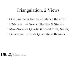
Downloaded 27 times

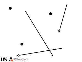
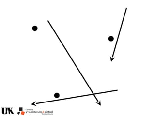
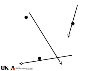
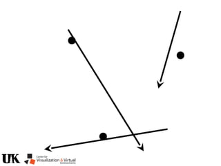
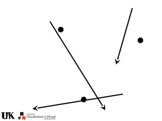
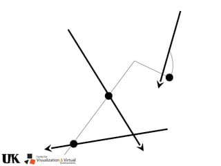
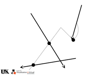
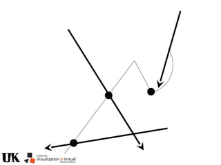
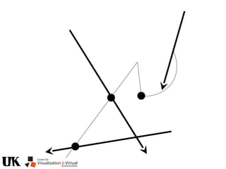
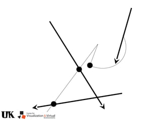
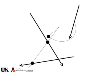
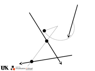
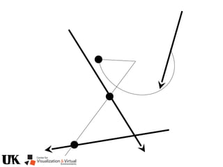
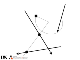
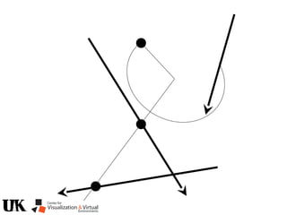
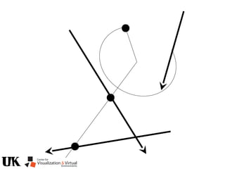
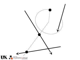
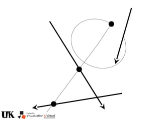
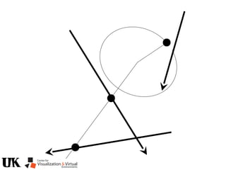
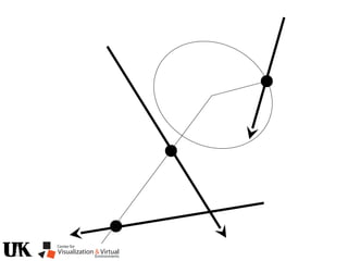
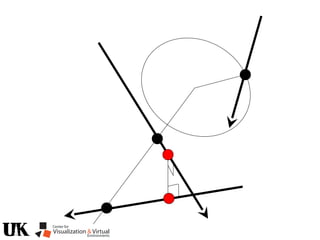
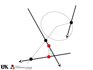
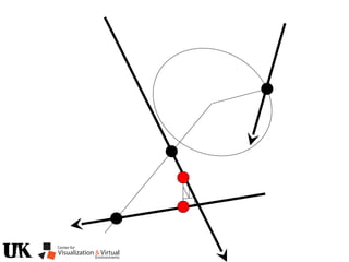
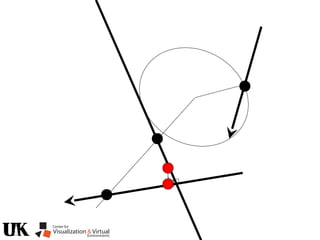
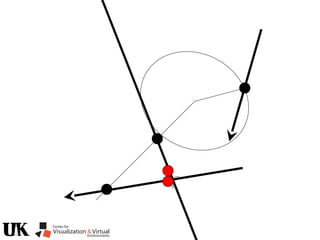
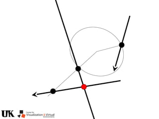
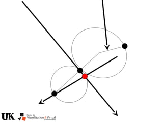
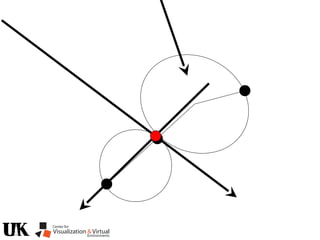
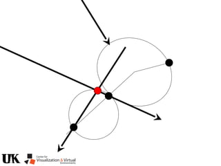
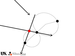
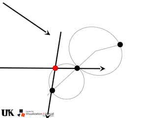
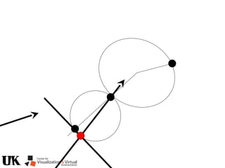
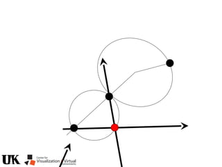
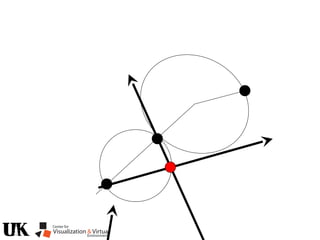
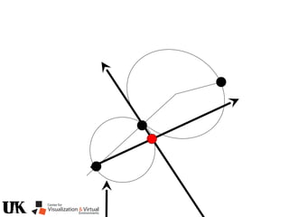
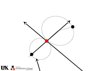
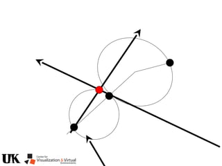
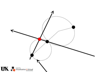
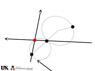
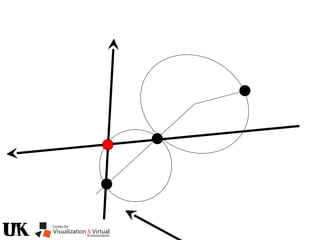
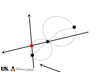
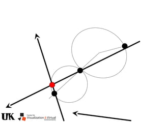
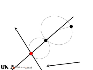
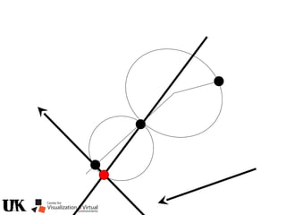
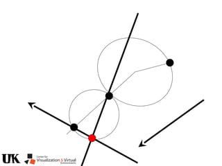
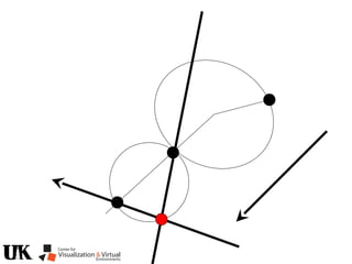
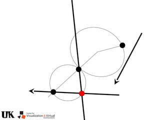
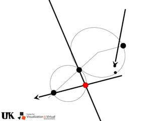
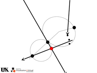
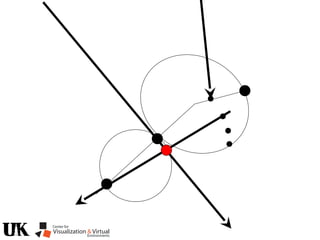
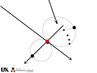
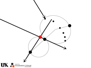
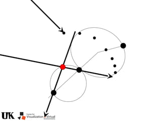
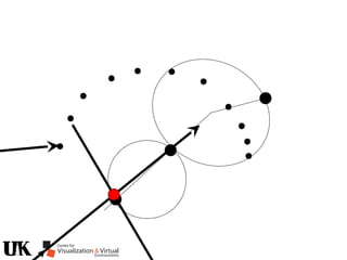
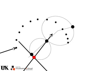
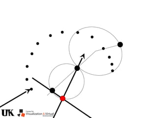
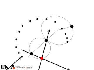
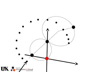
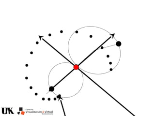
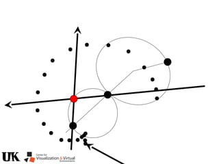
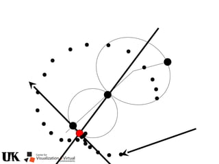
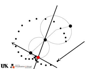
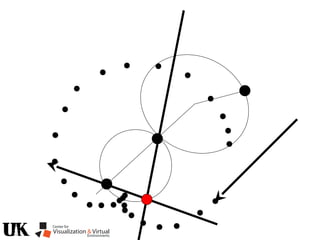
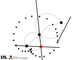
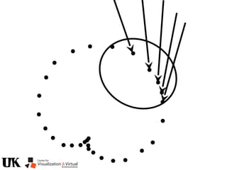
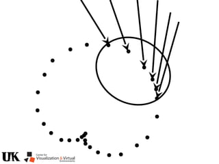
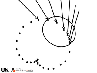
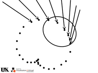
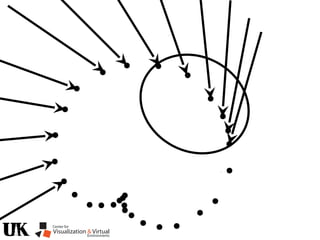
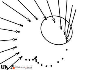
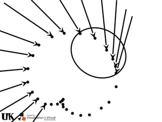
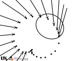
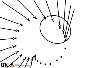
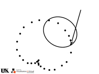
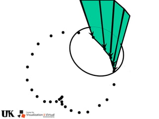
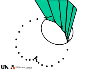
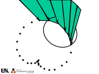
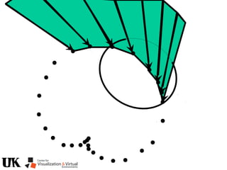
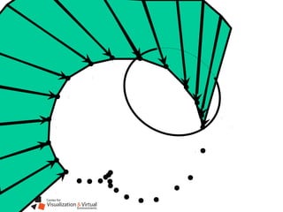
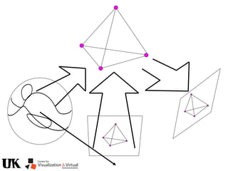
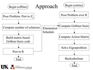
![Bezout’s Theorem
2x2=4
Mixed Volume, see for example [CLO 1998]
provides a generalization for non-general polynomials.
With two variables,
a solution according to
the Bezout bound
can typically be
realized with resultants.
With three or more
variables, things
are less simple.](https://image.slidesharecdn.com/nistericcv2005tutorial-101110003401-phpapp01/85/Nister-iccv2005tutorial-6-320.jpg)
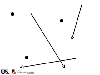
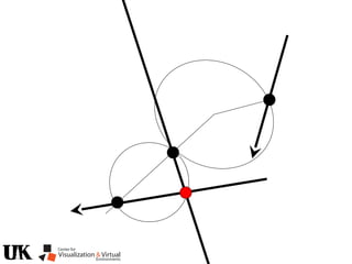
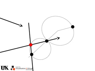
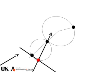
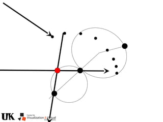
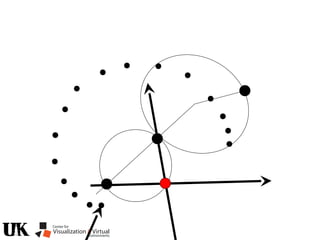
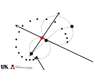
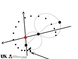
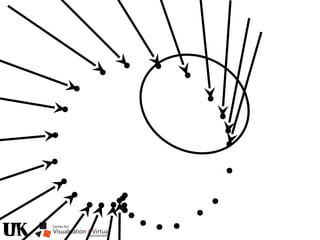
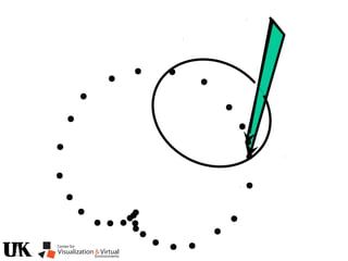
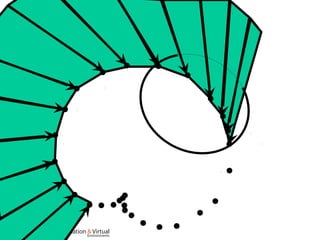
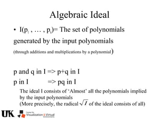
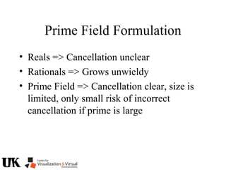
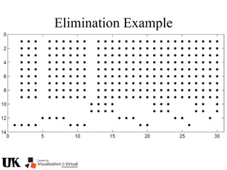
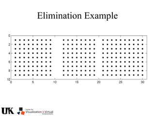
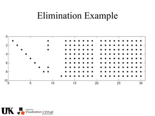
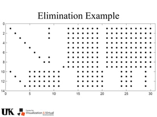
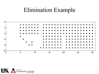
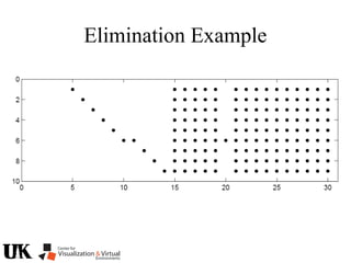
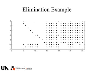
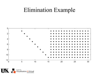
![Resultants
• Provides Elimination
of variables by taking
a determinant
]2[]1[]0[
]2[]1[]0[
]2[]1[]0[
]2[]1[]0[
1xx2
x3
= det = [4]
a1x2
+a2y2
+a3xy+a4x+a5y+a6
b1x2
+b2y2
+b3xy+b4x+b5y+b6
+++
+++
+++
+++
65
2
2431
65
2
2431
65
2
2431
65
2
2431
bybybbybb
bybybbybb
ayayaayaa
ayayaayaa
det
1xx2
x3](https://image.slidesharecdn.com/nistericcv2005tutorial-101110003401-phpapp01/85/Nister-iccv2005tutorial-7-320.jpg)


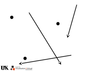
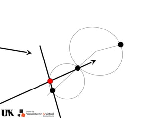
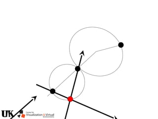

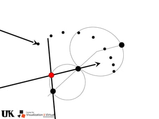
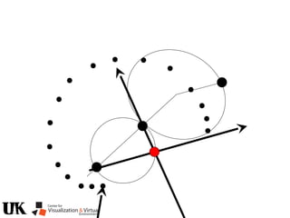
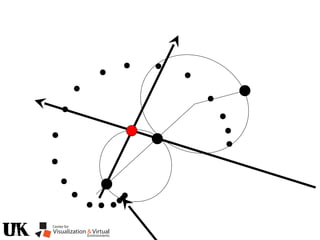
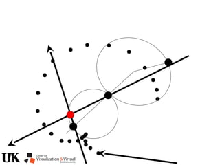

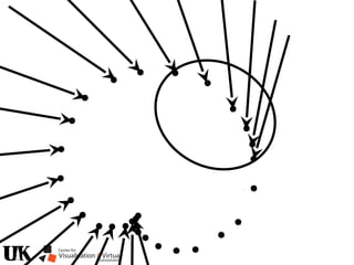

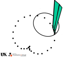


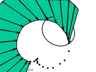


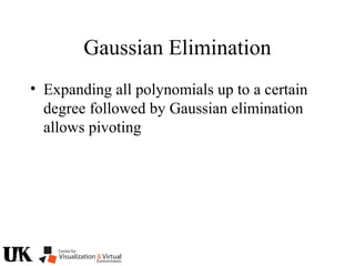
![Polynomial Formulation
• p1(x) , … , pn(x)= A set of input polynomials
(n polynomials in m variables)
x=[y1 … ym]](https://image.slidesharecdn.com/nistericcv2005tutorial-101110003401-phpapp01/85/Nister-iccv2005tutorial-223-320.jpg)
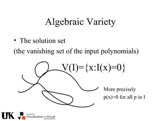
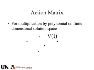
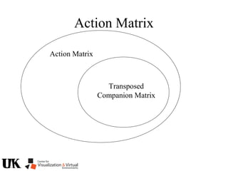

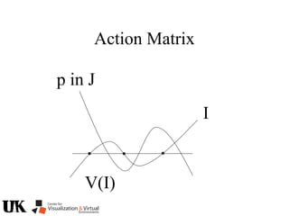
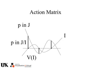
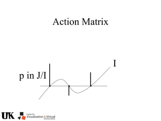
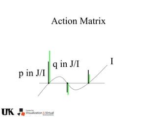
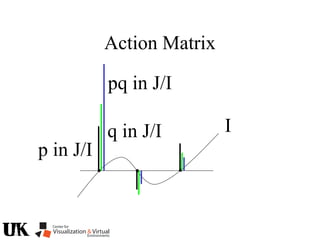
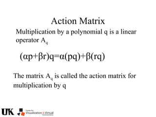
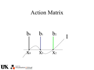
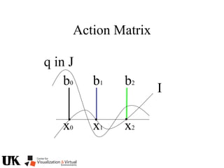
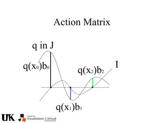
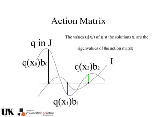
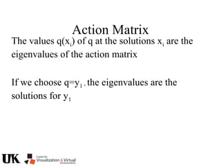
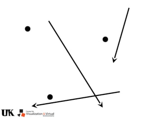
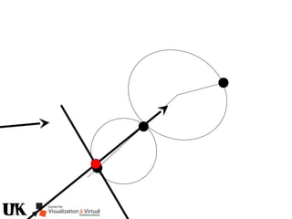
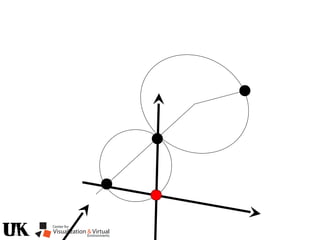
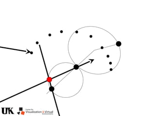
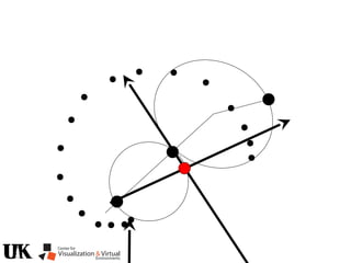
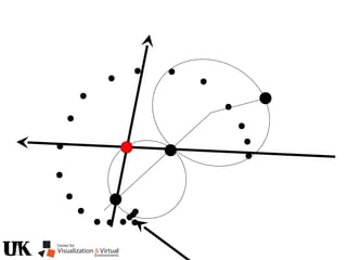
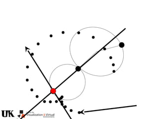
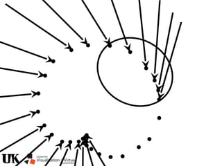
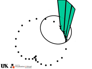
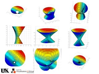
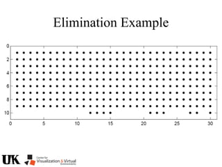
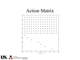
![Action Matrix
b’(x)Aq p=q(x)b’(x)p
for all p in J/I and x in V(I)
b’=[r1 … ro]
b’(x)Aq =b’(x)q(x)
b(x) is a left nullvector of Aq corresponding to eigenvalue q(x)](https://image.slidesharecdn.com/nistericcv2005tutorial-101110003401-phpapp01/85/Nister-iccv2005tutorial-246-320.jpg)
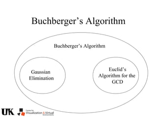
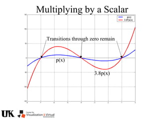
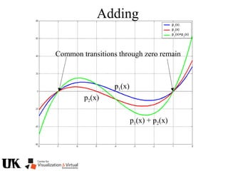
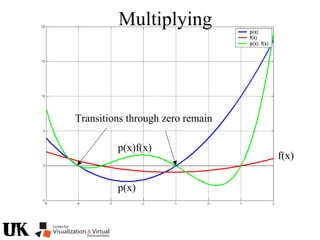
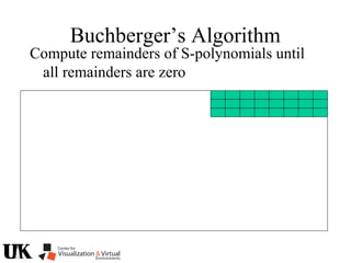


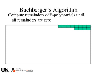
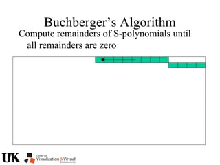
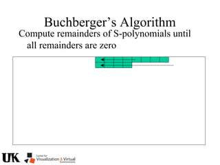
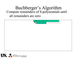


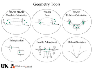
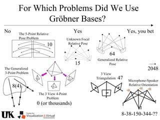
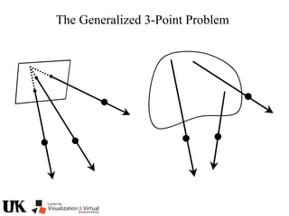
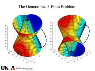
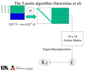
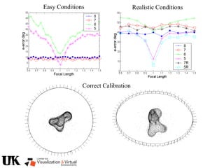
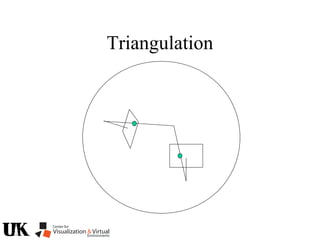
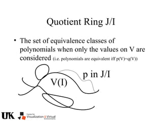
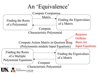
The document describes a tutorial on using algebraic geometry and Gröbner bases to solve polynomial problems in computer vision. The tutorial will cover the theory of Gröbner bases and how it can be used to solve systems of polynomial equations. Several examples of problems in computer vision that have been solved using Gröbner bases will be presented, including the generalized 3-point problem, 5-point relative pose problem, and triangulation. The tutorial aims to explain both the theoretical foundations and practical applications of Gröbner bases.