Downloaded 68 times


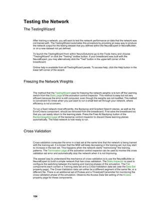

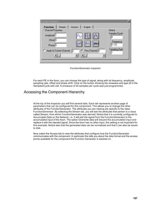
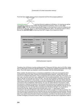
![The correlation coefficient is confined to the range [-1,1]. When r =1 there is a perfect positive linear
correlation between x and d, that is, they covary, which means that they vary by the same amount.
When r=-1, there is a perfectly linear negative correlation between x and d, that is, they vary in
opposite ways (when x increases, d decreases by the same amount). When r =0 there is no
correlation between x and d, i.e. the variables are called uncorrelated. Intermediate values describe
partial correlations. For example a correlation coefficient of 0.88 means that the fit of the model to
the data is reasonably good.
In NeuroSolutions, a correlation vector is created by attaching a probe to the Correlation access
point of the ErrorCriterion component.
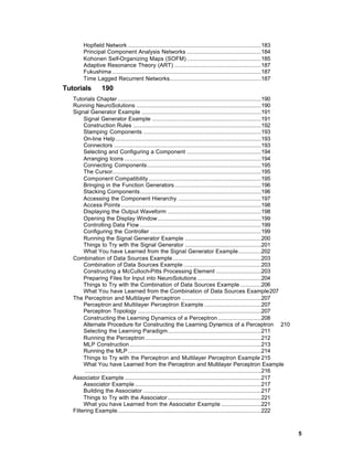
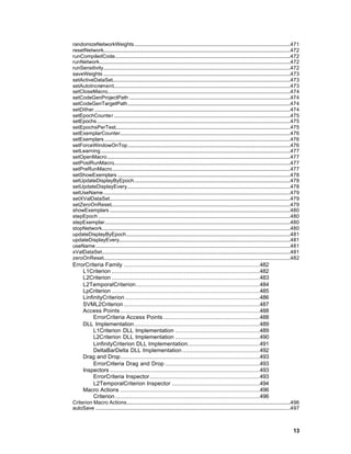
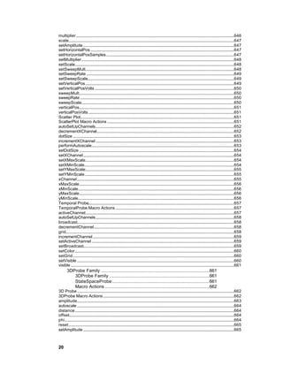
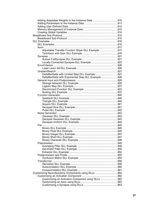
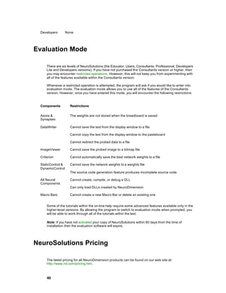
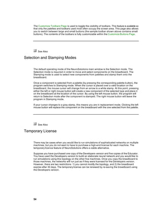
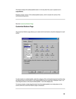
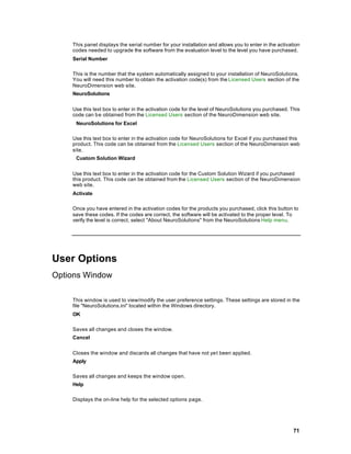
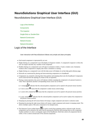
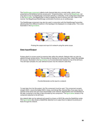
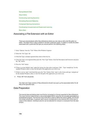
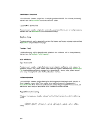
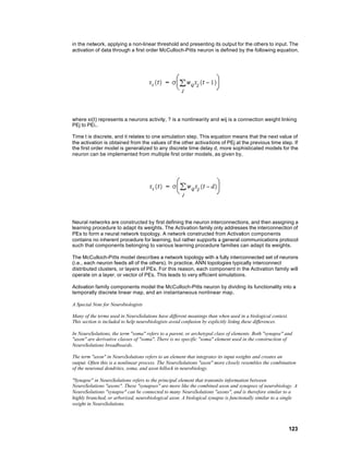
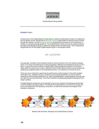
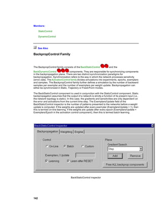
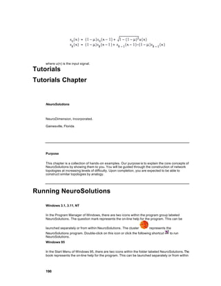
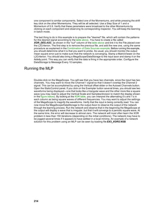
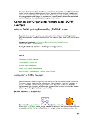
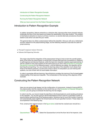
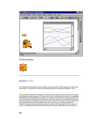
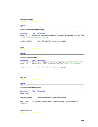
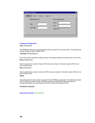
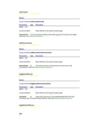
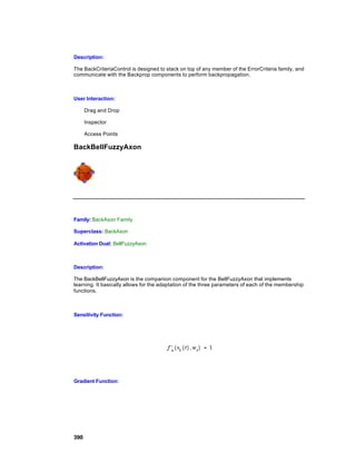
ROC Matrix
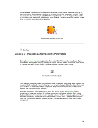
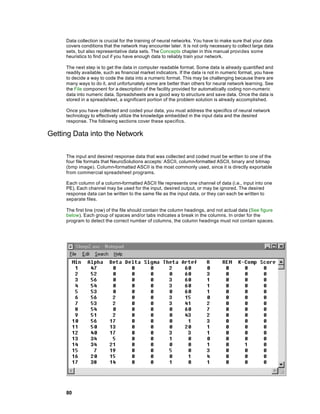
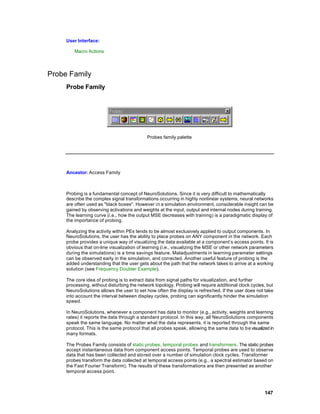
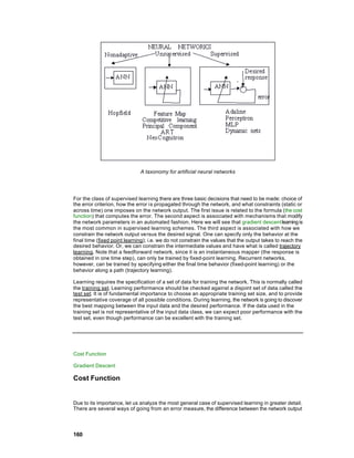
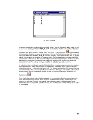
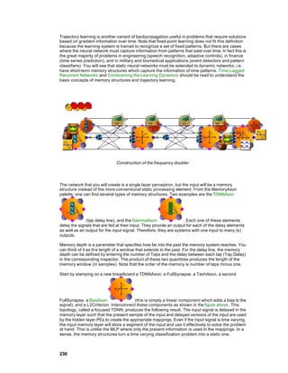
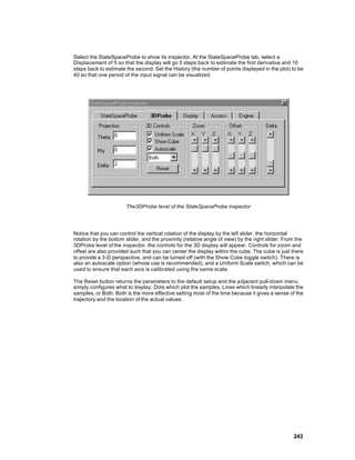
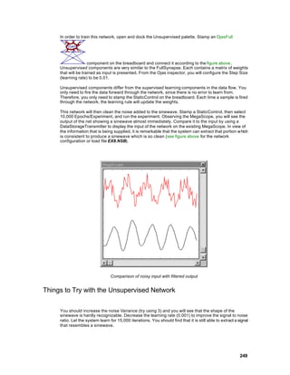
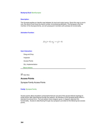
Receiver Operating Characteristic (ROC) matricies are used to show how changing the detection
threshold affects detections versus false alarms. If the threshold is set too high then the system will
miss too many detections. Conversely, if the threshold is set too low then there will be too many
false alarms. Below is an example of an ROC matrix graphed as an ROC curve.
Example ROC Curve
107](https://image.slidesharecdn.com/neurosolutionshelp-090922003656-phpapp01/85/NeuroDimension-Neuro-Solutions-HELP-107-320.jpg)


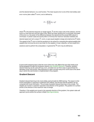
![Introduction to Neural Computation
Introduction to NeuroComputation
History of Neural Networks
What are Artificial Neural Networks
Neural Network Solutions
History of Neural Networks
Neural Networks are an expanding and interdisciplinary field bringing together mathematicians,
physicists, neurobiologists, brain scientists, engineers, and computer scientists. Seldom has a field
of study coalesced from so much individual expertise, bringing a tremendous momentum to neural
network research and creating many challenges.
One unsolved challenge in this field is the definition of a common language for neural network
researchers with very different backgrounds. Another, to compile a list of key papers which pleases
everyone, has only recently been accomplished, see Arbib, 1995. However, for the sake of
pragmatism, we present some key landmarks below.
Neural network theory started with the first discoveries about brain cellular organization, by Ramon
Y. Cajal and Charles S. Sherrington at the turn of the century. The challenge was immediately
undertaken to discover the principles that would make a complex interconnection of relatively
simple elements produce information processing at an intelligent level. This challenge is still with us
today.
The work of the neuroanatomists has grown into a very rich field of science cataloguing the
interconnectivity of the brain, its physiology and biochemistry [Eccles, Szentagothai], and its
function [Hebb]. The work of McCulloch and Pitts on the modeling of the neuron as a threshold
logic unit, and Caia-niello on neurodynamics merit special mention because they respectively led to
the analysis of neural circuits as switching d evices and as nonlinear dynamic systems. More
recently, brain scientists began studying the underlying principles of brain function [Braitenberg,
Marr, Pellionisz, Willshaw, Rumelhart, Freeman, Grossberg], and even implications to philosophy
[Churchland].
n Key books are Freeman’s "Mass Activation of the Nervous System", Eccles et al "The Cerebellum as a Neural
Machine", Shaw and Palm’s "Brain theory" (collection of key papers), Churchland "NeuroPhilosophy", and
Sejnowski and Churchland "The Computational Brain".
The theoretical neurobiologists’ work also interested computer scientists and engineers. The
principles of computation involved in the interconnection of simple elements led to cellular
automata [Von Neumann], were present in Norbert Wiener’s work on cybernetics and laid the
ground for artificial intelligence [Minsky, Arbib]. This branch is often referred to as artificial neural
networks, and will be the one reviewed here.
n There are a few compilations of key papers on ANN’s, for the technically motivated reader. We mention the
MIT Press Neuro Computing III, the IEEE Press Artificial Neural Networks and the book on Parallel models of
Associative memories by Erlbaum.
152](https://image.slidesharecdn.com/neurosolutionshelp-090922003656-phpapp01/85/NeuroDimension-Neuro-Solutions-HELP-152-320.jpg)
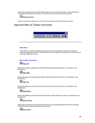
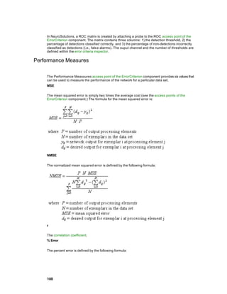
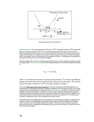
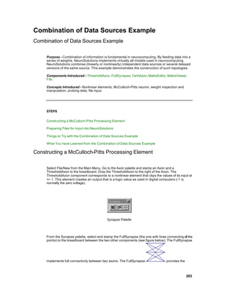
![n Patrick Simpson’s book has an extensive reference list of key papers, and provides one possible taxonomy of
neural computation.
n The DARPA book provides an early account of neural network applications and issues.
n Several books present the neural network computation paradigm at different technical levels:
n Hertz, Krogh and Palmer’s "Introduction to the Theory of Neural Computation" (Addison Wesley, 1991) has
probably one of the most thorough coverages of neural models, but requires a strong mathematical background.
n Zurada’s "Introduction to Artificial Neural Systems" (West, 1992) and Kung’s "Digital Neural Networks"
(Prentice Hall) are good texts for readers with an engineering background. Haykin’s book is encyclopedic,
providing an extensive coverage of neural network theory and its links to signal processing.
n An intermediate text is the Rumelhart and McClelland PDP Edition from MIT Press.
n Freeman and Skapura, and Caudill and Butler are two recommended books for the least technically oriented
reader.
n In terms of magazines with state-of-the art technical papers, we mention "Neural Computation", "Neural
Networks" and "IEEE Trans. Neural Networks".
n Proceedings of the NIPS (Neuro Information Processing Systems) Conference, the Snowbird Conference, the
Joint Conferences on Neural Networks and the World Congress are valuable sources of up-to-date technical
information.
An initial goal in neural network development was modeling memory as the collective property of a
group of processing elements [von der Marlburg, Willshaw, Kohonen, Anderson, Shaw, Palm,
Hopfield, Kosko]. Caianiello, Grossberg and Amari studied the principles of neural dynamics.
Rosenblatt created the perceptron for data driven (nonparametric) pattern recognition, and
Fukushima, the cognitron. Widrow’s adaline (adaptive linear element) found applications and
success in communication systems. Hopfield’s analogy of computation as a dynamic process
captured the importance of distributed systems. Rumelhart and McClelland’s compilation of papers
in the PDP (Parallel Distributive Processing) book, opened up the field for a more general
audience. From the first International Joint Conference on Neural Networks held in San Diego,
1987, the field exploded.
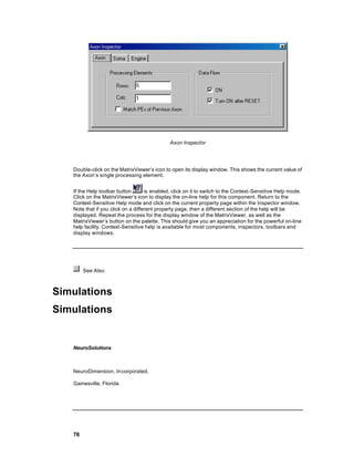
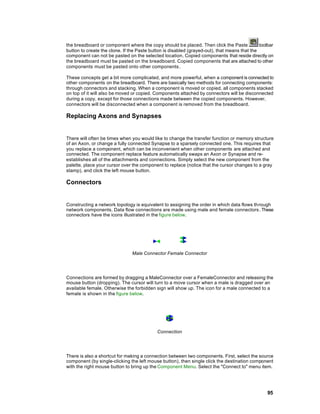
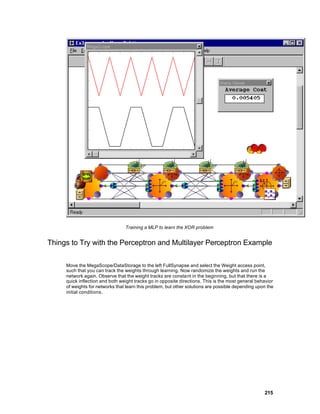
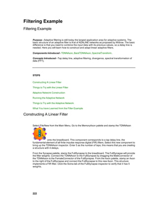
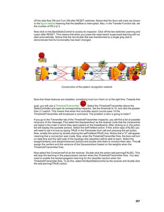
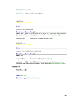
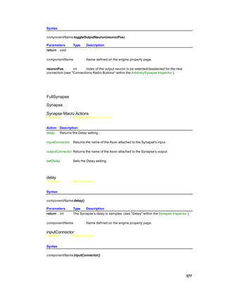
What are Artificial Neural Networks
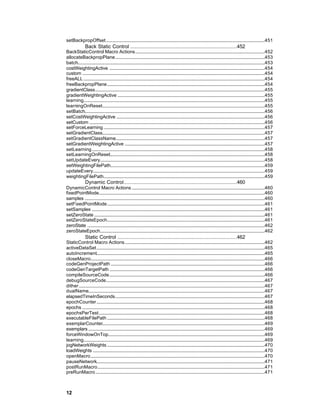
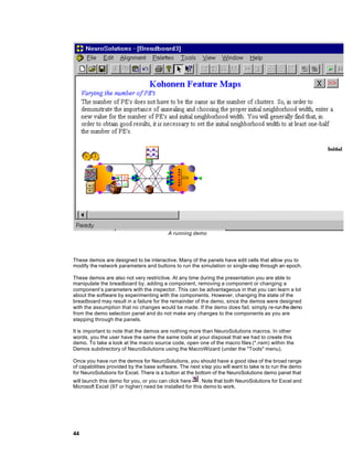
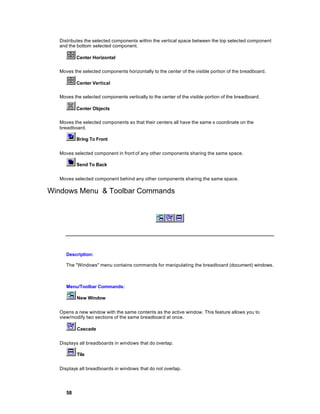
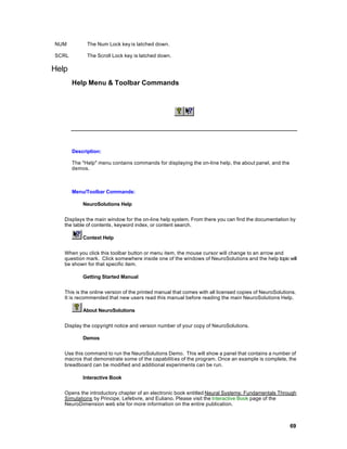
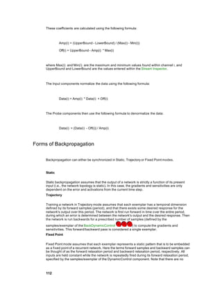
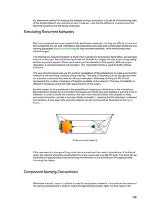
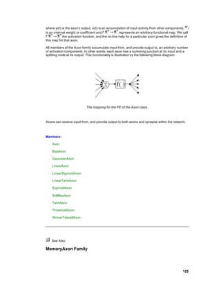
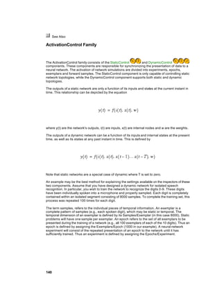
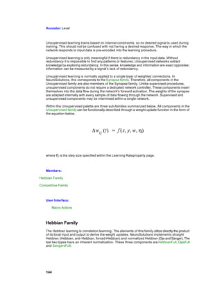
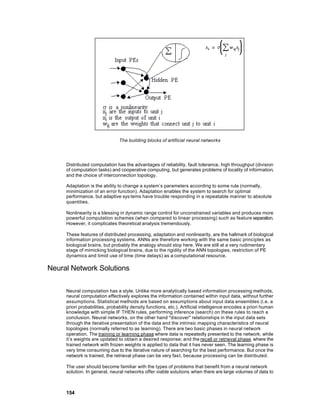
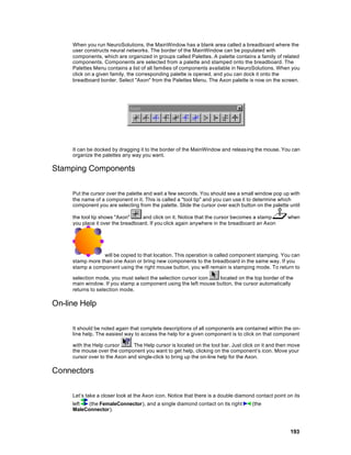
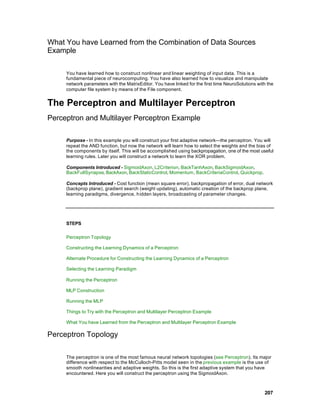
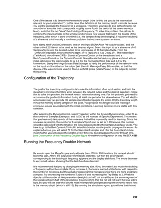
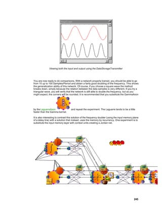
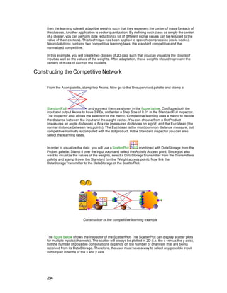
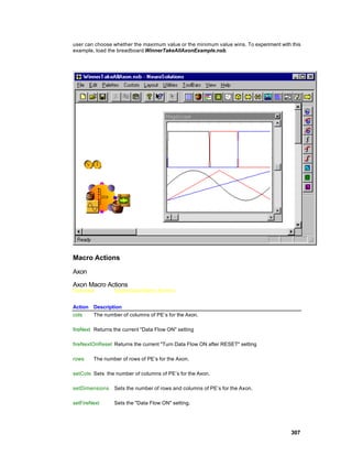
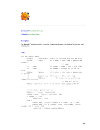
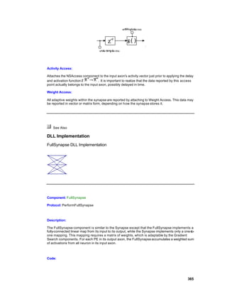
Artificial neural networks (ANN) are highly distributed interconnections of adaptive nonlinear
processing elements (PEs). When implemented in digital hardware, the PE is a simple sum of
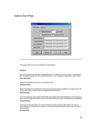
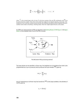
products followed by a nonlinearity (McCulloch-Pitts neuron). An artificial neural network is nothing
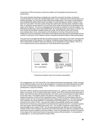
but a collection of interconnected PEs (see figure below). The connection strengths, also called the
network weights, can be adapted such that the network’s output matches a desired response.
153](https://image.slidesharecdn.com/neurosolutionshelp-090922003656-phpapp01/85/NeuroDimension-Neuro-Solutions-HELP-153-320.jpg)
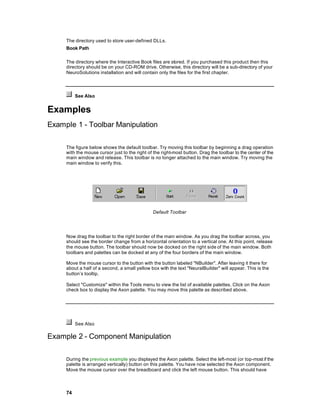
![train the neural network. When a problem is difficult (or impossible) to formulate analytically and
experimental data can be obtained, then a neural network solution is normally appropriate.
The major applications of ANNs are the following:
Pattern classifiers: The necessity of a data set in classes is a very common problem in information processing.
We find it in quality control, financial forecasting, laboratory research, targeted marketing, bankruptcy
prediction, optical character recognition, etc. ANNs of the feedforward type, normally called multilayer
perceptrons (MLPs) have been applied in these areas because they are excellent functional mappers (these
problems can be formulated as finding a good input-output map). The article by Lippman is an excellent
review of MLPs.
Associative memories: Human memory principles seem to be of this type. In an associative memory, inputs
are grouped by common characteristics, or facts are related. Networks implementing associative memory
belong generally to the recurrent topology type, such as the Hopfield network or the bidirectional associative
memory. However, there are simpler associative memories such as the linear or nonlinear feedforward
associative memories. A good overview of associative memories is a book edited by Anderson et al,
Kohonen’s book (for the more technically oriented), or Freeman and Skapura book for the beginner.
Feature extractors: This is also an important building block for intelligent systems. An important aspect of
information processing is simply to use relevant information, and discard the rest. This is normally
accomplished in a pre-processing stage. ANNs can be used here as principal component analyzers, vector
quantizers, or clustering networks. They are based on the idea of competition, and normally have very simple
one-layer topologies. Good reviews are presented in Kohonen’s, and in Hertz et al book.
Dynamic networks: A number of important engineering applications require the processing of time-varying
information, such as speech recognition, adaptive control, time series prediction, financial forecasting,
radar/sonar signature recognition and nonlinear dynamic modeling. To cope with time varying signals, neural
network topologies have to be enhanced with short term memory mechanisms. This is probably the area
where neural networks will provide an undisputed advantage, since other technologies are far from
satisfactory. This area is still in a research stage. The books of Hertz and Haykin present a reasonable
overview, and the paper of deVries and Principe covers the basic theory.
Notice that a lot of real world problems fall in this category, ranging from classification of irregular
patterns, forecasting, noise reduction and control applications. Humans solve problems in a very
similar way. They observe events to extract patterns, and then make generalizations based on their
observations.
Neural Network Analysis
Neural Network Analysis
At the highest level of neural network analysis is the neural model. Neural models represent
dynamic behavior. What we call neural networks are nothing but special topologies (realizations) of
neural models.
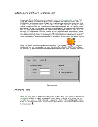
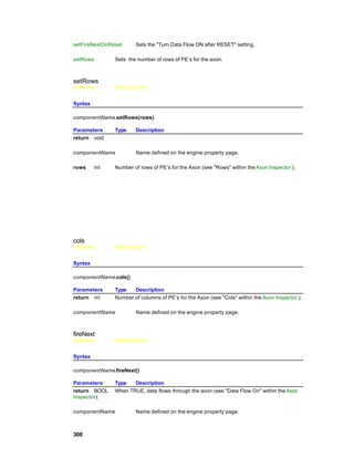
The most common neural model is the additive model [Amari, Grossberg, Carpenter]. The neurodynamical
equation is
155](https://image.slidesharecdn.com/neurosolutionshelp-090922003656-phpapp01/85/NeuroDimension-Neuro-Solutions-HELP-155-320.jpg)


![for multiple layer networks (this phenomenon is sometimes called error dispersion). Fahlman
proposes adding a small constant (0.1) to the propagated error to speed up learning.
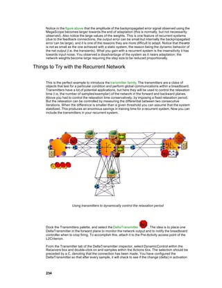
Constraining the Learning Dynamics
Constraining the Learning Dynamics
Feedforward networks only accept fixed-point learning algorithms because the network reaches a
steady state in one iteration (instantaneous mappers). Due to this absence of dynamics,
feedforward networks are also called static networks. Backpropagation for these networks is a
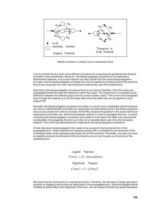
static learning rule and is therefore referred to as static backpropagation. In recurrent networks, the
learning problem is slightly more complex due to the richer dynamic behavior of the networks.
One may want to teach a recurrent network a static output. In this case the learning paradigm is still
fixed point learning, but since the network is recurrent it is called recurrent backpropagation.
Almeida and Pineda showed how static backpropagation could be extended to this case. Using the
transpose network, fixed-point learning can be implemented with the backpropagation algorithm,
but the network dynamics MUST die away. The method goes as follows: An input pattern is
presented to the recurrent net. The network state will evolve until the output stabilizes (normally a
predetermined number of steps). Then the output error (difference between the stable output and
the desired behavior) can be computed and propagated backwards through the adjoining network.
The error must also settle down, and once it stabilizes, the weights can be adapted using the static
delta rule presented above. This process is repeated for every one of the training patterns and as
many times as necessary. NeuroSolutions implements this training procedure.
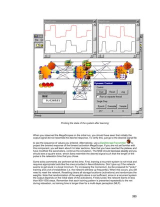
In some cases the network may fail to converge due to instability of the network dynamics. This is
an unresolved issue at this time. We therefore recommend extensive probing of recurrent networks
during learning.
The other learning paradigm is trajectory learning where the desired signal is not a point but a
sequence of points. The goal in trajectory learning is to constrain the system output during a period
of time (therefore the name trajectory learning). This is particularly important in the classification of
time varying patterns when the desired output occurs in the future; or when we want to approximate
a desired signal during a time segment, as in multistep prediction. The cost function in trajectory
learning becomes
where T is the length of the training sequence and i is the index of output units.
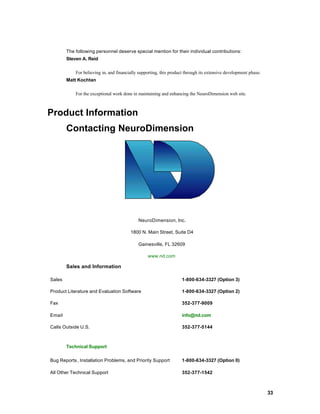
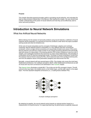
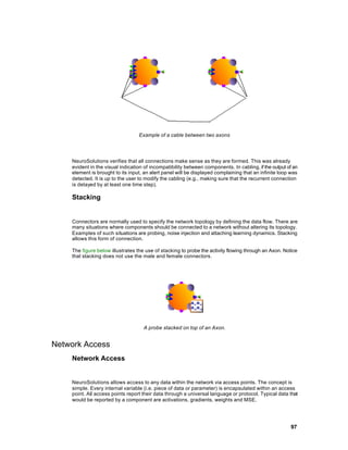
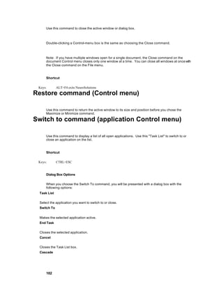
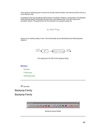
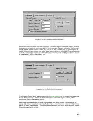
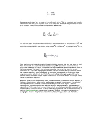
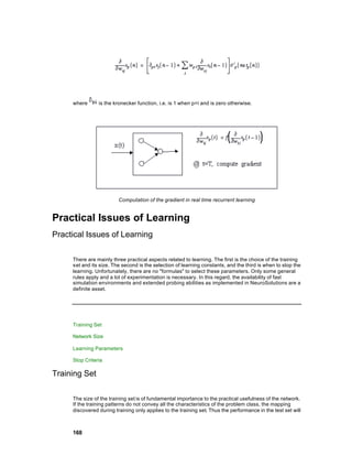
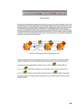
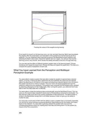
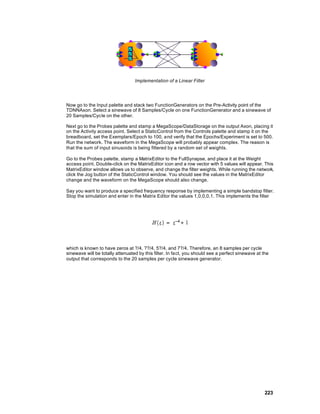
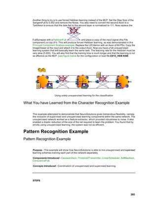
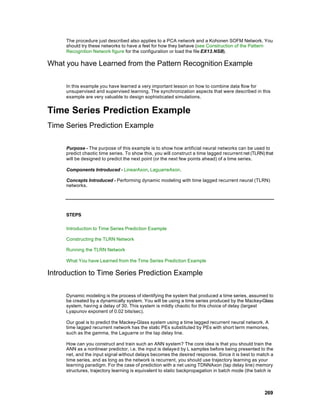
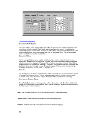
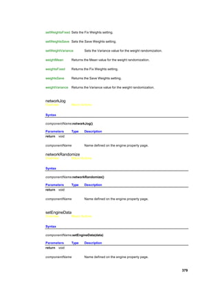
The ANN literature provides basically two procedures to learn through time: the backpropagation
through time algorithm (BPTT) and the real time recurrent learning algorithm (RTRL).
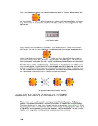
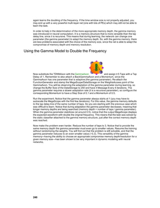
In BPTT the idea is the following [Rumelhart and Williams, Werbos]: the network has to be run
forward in time until the end of the trajectory and the activation of each PE must be stored locally in
a memory structure for each time step. Then the output error is computed, and the error is
backpropagated across the network (as in static backprop) AND the error is backpropagated
through time (see figure below). In equation form we have,
166](https://image.slidesharecdn.com/neurosolutionshelp-090922003656-phpapp01/85/NeuroDimension-Neuro-Solutions-HELP-166-320.jpg)
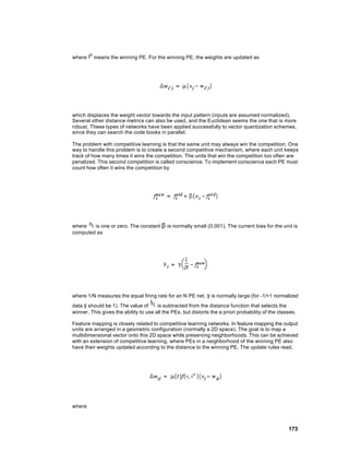
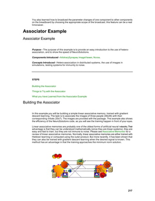
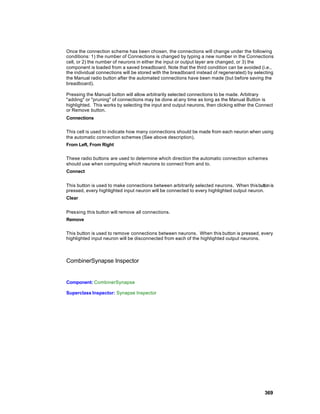
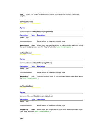
![where (n) is the error propagated by the transpose network across the network and through
time. Since the activations x(n) in the forward pass have been stored, the gradient across time can
be reconstructed by simple addition. This procedure is naturally implemented in NeuroSolutions.
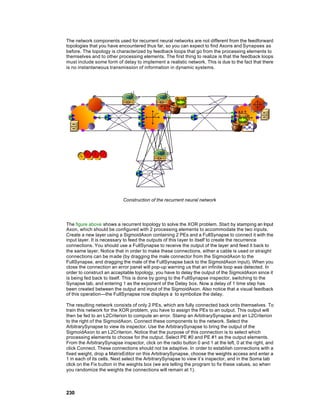
Construction of the gradient in Backpropagation through time.
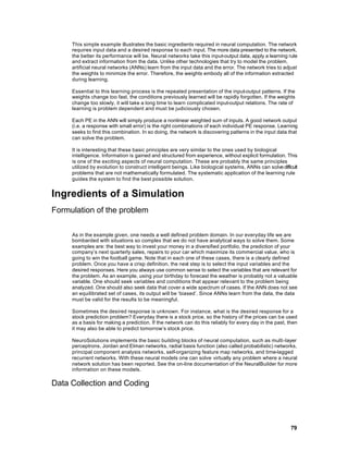
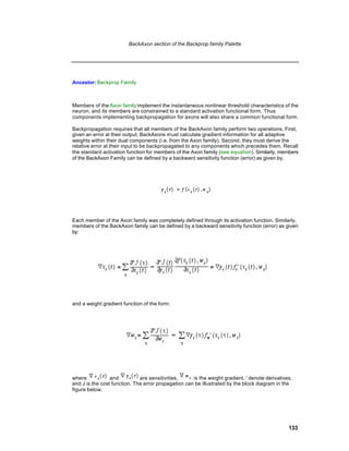
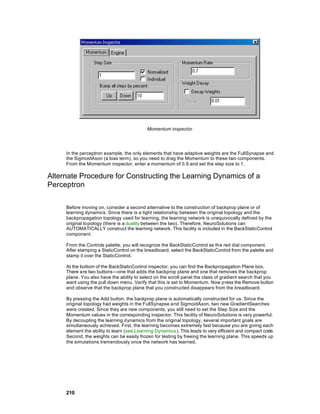
The other procedure for implementing trajectory learning is based on a very different concept. It is
called real time recurrent learning [Williams and Zipser] and is a natural extension of the gradient
computation in adaptive signal processing and control theory. The idea is to compute, at each time
step, ALL the sensitivities, i.e. how much a change in one weight will affect the activation of all the
PEs of the network. Since there are weights in a fully connected net, and for each we have to
keep track of N derivatives this is a very computationally intensive procedure (we further need N
multiplications to compute each gradient). However, notice that we can perform the computation at
each time step, so the storage requirements are not a function of the length of the trajectory. At the
end of the trajectory, we can multiply these sensitivities by the error signal and compute the
gradient along the trajectory (see figure below). In equation form we write the gradient as
where (n) is the output of the network. We can compute the derivative of the activation
recursively as
167](https://image.slidesharecdn.com/neurosolutionshelp-090922003656-phpapp01/85/NeuroDimension-Neuro-Solutions-HELP-167-320.jpg)
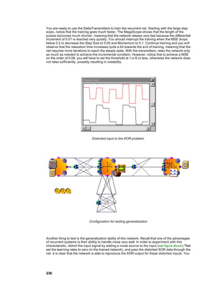
![be much worse than the training set performance. The only general rules that can be formulated
are to use a lot of data and use representative data. If you do not have lots of data to train the ANN,
then the ANN paradigm is probably not the best solution to solve your problem. Understanding of
the problem to be solved is of fundamental importance in this step.
Another aspect of proper training is related to the relation between training set size and number of
weights in the ANN. If the number of training examples is smaller than the number of weights, one
can expect that the network may "hard code" the solution, i.e. it may allocate one weight to each
training example. This will obviously produce poor generalization (i.e the ability to link unseen
examples to the classes defined from the training examples). We recommend that the number of
training examples be at least double the number of network weights.
When there is a big discrepancy between the performance in the training set and test set, we can
suspect deficient learning. Note that one can always expect a drop in performance from the training
set to the test set. We are referring to a large drop in performance (more than 10~15%). In cases
like this we recommend increasing the training set size and/or produce a different mixture of
training and test examples.
Network Size
At our present stage of knowledge, establishing the size of a network is more efficiently done
through experimentation. The theory of generalization addresses this issue, but it is still difficult to
apply in practical settings [VP dimension, Vapnik]. The issue is the following: The number of PEs in
the hidden layer is associated with the mapping ability of the network. The larger the number, the
more powerful the network is. However, if one continues to increase the network size, there is a
point where the generalization gets worse. This is due to the fact that we may be over-fitting the
training set, so when the network works with patterns that it has never seen before the response is
unpredictable. The problem is to find the smallest number of degrees of freedom that achieves the
required performance in the TEST set.
One school of thought recommends starting with small networks and increasing their size until the
performance in the test set is appropriate. Fahlman proposes a method of growing neural
topologies (the cascade correlation) that ensures a minimal number of weights, but the training can
be fairly long. An alternate approach is to start with a larger network, and remove some of the
weights. There are a few techniques, such as weight decay, that partially automate this idea
[Weigend, LeCun]. The weights are allowed to decay from iteration to iteration, so if a weight is
small, its value will tend to zero and can be eliminated.
In NeuroSolutions the size of the network can be controlled by probing the hidden layer weight
activations with the scopes. When the value of an activation is small, does not change during
learning, or is highly correlated with another activation, then the size of the hidden layer can be
decreased.
Learning Parameters
The control of the learning parameters is an unsolved problem in ANN research (and for that matter
in optimization theory). The point is that one wants to train as fast as possible and reach the best
performance. Increasing the learning rate parameter will decrease the training time, but will also
increase the possibility of divergence, and of rattling around the optimal value. Since the weight
correction is dependent upon the performance surface characteristics and learning rate, to obtain
constant learning, an adaptive learning parameter is necessary. We may even argue that what is
necessary is a strategy where the learning rate is large in the beginning of the learning task and
progressively decays towards the end of adaptation. Modification of learning rates is possible under
certain circumstances, but a lot of other parameters are included that also need to be
experimentally set. Therefore, these procedures tend to be brittle and the gains are problem
dependent (see the work of Fahlman, LeCun, and Silva and Almeida, for a review). NeuroSolutions
169](https://image.slidesharecdn.com/neurosolutionshelp-090922003656-phpapp01/85/NeuroDimension-Neuro-Solutions-HELP-169-320.jpg)
![enables versatile control of the learning rates by implementing adaptive schemes [Jacob] and
Fahlman’s quickprop [Fahlman].
The conventional approach is to simply choose the learning rate and a momentum term. The
momentum term imposes a "memory factor" on the adaptation, and has been shown to speedup
adaptation while avoiding local minima trapping to a certain extent. Thus, the learning equation
becomes
where γ is a constant (normally set between 0.5 and 0.9), and µ is the learning rate.
Jacob’s delta bar delta is also a versatile procedure, but requires more care in specification of the
learning parameters . The idea is the following: when there are consecutive iterations that produce
the same sign of weight update, the learning rate is too small. On the other hand, if consecutive
iterations produce weight updates that have opposite signs, the learning rate is too fast. Jacob
proposed the following formulas for learning rate updates:
where η is the learning rate for each weight, (n) is the gradient and
where ξ is a small constant.
One other option available to the researcher is when to perform the weight updates. Updates can
be performed at the end of presentation of all the elements of the training set (batch learning) or at
each iteration (real time). The first modality "smoothes" the gradient and may give faster learning
for noisy data, however it may also average the gradient to zero and stall learning. Modification of
the weights at each iteration with a small learning rate may be preferable most of the time.
Stop Criteria
The third problem is how to stop the learning. Stop criteria are all based on monitoring the mean
square error. The curve of the MSE as a function of time is called the learning curve. The most
used criterion is probably to choose the number of iterations, but we can also preset the final error.
170](https://image.slidesharecdn.com/neurosolutionshelp-090922003656-phpapp01/85/NeuroDimension-Neuro-Solutions-HELP-170-320.jpg)

![and y (the input and output of the weight). This principle can even be applied with the input and a
desired signal, as in heteroassociation (forced Hebbian).
A very effective normalization of the Hebbian rule has been proposed by Oja, and reads
For linear networks, one can show that Oja’s rule finds the principal component o f the input data,
i.e. it implements what is called an eigenfilter. A common name for the eigenfilter is matched filter,
which is known to maximize the signal to noise ratio. Hence, Oja’s rule produces a system that is
optimal and can be used for feature e xtraction.
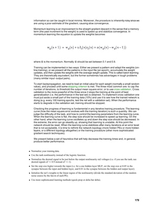
This network can be extended to M multiple output units and extract, in order, the M principal
components of the input [Sanger], yielding
where
Principal Component Analysis is a very powerful feature representation method. PCA projects the
data cluster on a set of orthogonal axes that best represent the input at each order. It can be shown
that PCA is solving an eigenvalue problem. This can be accomplished with linear algebra
techniques, but here we are doing the same thing using on-line, adaptive techniques.
Another unsupervised learning paradigm is competitive learning. The idea of competitive learning is
that the output PEs compete to be on all the time (winner-take-all). This is accomplished by
creating inhibitory connections among the output PEs. Competitive learning networks cluster the
input patterns, and can therefore be used in data reduction through vector quantization. One can
describe competitive learning as a sort of Hebbian learning applied to the output node that wins the
competition among all the output nodes. First, only one of the output units can be active at a given
time (called the winner), which is defi ned as the PE that has the largest summed input. If the
weights to each PE are normalized, then this choice takes the winner as the unit closest to the
input vector x in the norm sense, i.e.
172](https://image.slidesharecdn.com/neurosolutionshelp-090922003656-phpapp01/85/NeuroDimension-Neuro-Solutions-HELP-172-320.jpg)

![Dynamic Networks
Dynamic Networks
Dynamic networks are a very important class of neural network topologies that are able to process
time varying signals. They can be viewed as a nonlinear extension of adaptive linear filters, or an
extension of static neural networks to time varying inputs. As such they fill an increasingly important
niche in neural network applications and deserve special treatment in this introduction to neural
computation. NeuroSolutions was developed from the start with dynamic neural network
applications in mind.
A dynamic neural network is a static neural network with an extended memory mechanism, which
is able to store past values of the input signal. In many applications (system identification,
classification of patterns in time, nonlinear prediction) memory is important for allowing decisions
based on input behavior over a period of time. A static classifier makes decisions based on the
present input only; it can therefore not perform functions that involve knowledge about the history of
the input signal.
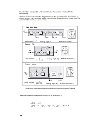
In neural networks, the most common memory structures are linear filters. In the time delay neural
network (TDNN) the memory is a tap delay line, i.e. a set of memory locations that store the past of
the input [Waibel]. Self-recurrent connections (feeding the output of a PE to the input) have also
been used as memory, and these units are called context units [Elman, Jordan].
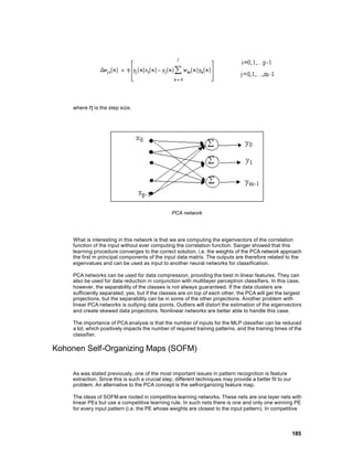
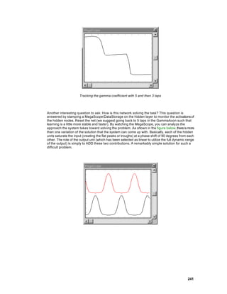
The gamma memory (see figure below) is a structure that cascades self-recurrent connections
[deVries and Principe]. It is therefore a structure with local feedback, that extends the context unit
with more versatile storage, and accepts the tap delay line as a special case (µ=1).
The gamma memory. gi(t) are inputs to the next layer PEs.
µ is an adaptive parameter that controls the depth of the memory. This structure has a memory
depth of K/µ, where K is the number of taps in the cascade. Its resolution is µ [deVries and
Principe]. Since this topology is recurrent, a form of temporal learning must be used to adapt the
gamma parameter µ (i.e. either real time recurrent learning or backpropagation through time). The
advantage of this structure in dynamic networks is that we can, with a predefined number of taps,
provide a controllable memory. And since the network adapts the gamma parameter to minimize
the output mean square error, the best compromise depth/resolution is achieved.
176](https://image.slidesharecdn.com/neurosolutionshelp-090922003656-phpapp01/85/NeuroDimension-Neuro-Solutions-HELP-176-320.jpg)
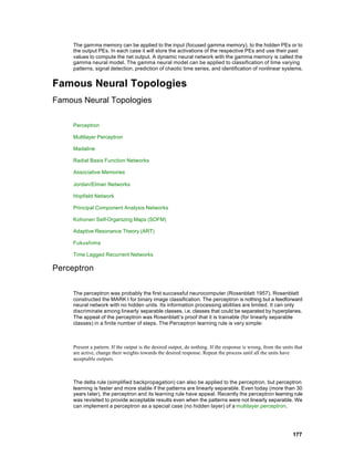
![Multilayer Perceptron
The multilayer perceptron (MLP) is one of the most widely implemented neural network topologies.
The article by Lippman is probably one of the best references for the computational capabilities of
MLPs. Generally speaking, for static pattern classification, the MLP with two hidden layers is a
universal pattern classifier. In other words, the discriminant functions can take any shape, as
required by the input data clusters. Moreover, when the weights are properly normalized and the
output classes are normalized to 0/1, the MLP achieves the performance of the maximum a
posteriori receiver, which is optimal from a classification point of view [Makhoul]. In terms of
mapping abilities, the MLP is believed to be capable of approximating arbitrary functions. This has
been important in the study of nonlinear dynamics [Lapedes and Farber], and other function
mapping problems.
MLPs are normally trained with the backpropagation algorithm [Rumelhart et al]. In fact the
renewed interest in ANNs was in part triggered by the existence of backpropagation. The LMS
learning algorithm proposed by Widrow can not be extended to hidden PEs, since we do not know
the desired signal there. The backpropagation rule propagates the errors through the network and
allows adaptation of the hidden PEs.
Two important characteristics of the multilayer perceptron are: its nonlinear processing elements
(PEs) which have a nonlinearity that must be smooth (the logistic function and the hyperbolic
tangent are the most widely used); and their massive interconnectivity (i.e. any element of a given
layer feeds all the elements of the next layer).
The multilayer perceptron is trained with error correction learning, which means that the desired
response for the system must be known. In pattern recognition this is normally the case, since we
have our input data labeled, i.e. we know which data belongs to which experiment.
Error correction learning works in the following way: From the system response at PE i at iteration
n, (n), and the desired response (n) for a given input pattern an instantaneous error (n) is
defined by
Using the theory of gradient descent learning, each weight in the network can be adapted by
correcting the present value of the weight with a term that is proportional to the present input and
error at the weight, i.e.
The local error (n) can be directly computed from (n) at the output PE or can be computed as a
weighted sum of errors at the internal PEs. The constant η is called the step size. This procedure is
called the backpropagation algorithm.
Backpropagation computes the sensitivity of a cost functional with respect to each weight in the
network, and updates each weight proportional to the sensitivity. The beauty of the procedure is
that it can be implemented with local information and requires just a few multiplications per weight,
which is very efficient. Because this is a gradient descent procedure, it only uses the local
178](https://image.slidesharecdn.com/neurosolutionshelp-090922003656-phpapp01/85/NeuroDimension-Neuro-Solutions-HELP-178-320.jpg)
![n Always have more training patterns than weights. You can expect the performance of your MLP in the test set
to be limited by the relation N>W/ε , where N is the number of training epochs, W the number of weights and ε
the performance error. You should train until the mean square error is less than ε /2.
Madaline
Madaline is an acronym for multiple adalines, the ADAptive LINear Element proposed by Widrow
[Widrow and Hopf]. The adaline is nothing but a linear combiner of static information, which is not
very powerful. However, when extended to time signals, the adaline becomes an adaptive filter of
the finite impulse response class. This type of filter was studied earlier by Wiener (1949). Widrow’s
contribution was the learning rule for training the adaptive filter. Instead of numerically solving the
equations to obtain the optimal value of the weights (the Wiener-Hopf solution), Widrow proposed a
very simple rule based on gradient descent learning (the least mean square rule LMS). The
previous adaptive theory was essentially statistical (it required expected value operators), but
Widrow took the actual value of the product of the error at each unit and its input as a rough
estimate of the gradient. It turns out that this estimate is noisy, but unbiased, so the number of
iterations over the data average the estimate and make it approach the true value.
The adaptive linear combiner with the LMS rule is one of the most widely used structures in
adaptive signal processing [Widrow and Stearns]. Its applications range from echo cancellation, to
line equalization, spectral estimator, beam former in adaptive antennas, noise canceller, and
adaptive controller. The adaline is missing one of the key ingredients for our definition of neural
networks (nonlinearity at the processing element), but it possesses the other two (distributed and
adaptive).
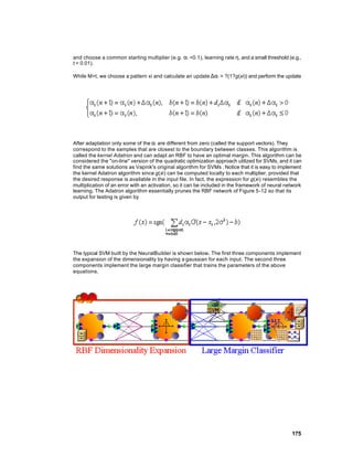
Radial Basis Function Networks
Radial basis functions networks have a very strong mathematical foundation rooted in
regularization theory for solving ill-conditioned problems. Suppose that we want to find the map that
transforms input samples into a desired classification. Due to the fact that we only have a few
samples, and that they can be noisy, the problem of finding this map may be very difficult
(mathematicians call it ill-posed). We want to solve the mapping by decreasing the error between
the network output and the desired response, but we want to also include an added constraint
relevant to our problem. Normally this constraint is smoothness.
One can show that such networks can be constructed in the following way (see figure below): Bring
every input component (p) to a layer of hidden nodes. Each node in the hidden layer is a p
multivariate Gaussian function
of mean (each data point) and variance . These functions are called radial basis functions.
Finally, linearly weight the output of the hidden nodes to obtain
180](https://image.slidesharecdn.com/neurosolutionshelp-090922003656-phpapp01/85/NeuroDimension-Neuro-Solutions-HELP-180-320.jpg)

![Steinbuch was a cognitive scientist and one of the pioneering researchers in distributed
computation. His interests were in associative memories, i.e. devices that could learn associations
among dissimilar binary objects. He implemented the learnmatrix, where a set of binary inputs is
fed to a matrix of resistors, producing a set of binary outputs. The outputs are 1 if the sum of the
inputs is above a given threshold, zero otherwise. The weights (which were binary) were updated
by using several very simple rules based on Hebbian learning. But the interesting thing is that the
asymptotic capacity of this network is rather high and easy to determine (I= [Willshaw]).
The linear associative memory was proposed by several researchers [Anderson, Kohonen]. It is a
very simple device with one layer of linear units that maps N inputs (a point in N dimensional
space) onto M outputs (a point in M dimensional space). In terms of signal processing, this network
does nothing but a projection operation of a vector in N dimensional s pace to a vector in M
dimensional space.
This projection is achieved by the weight matrix. The weight matrix can be computed analytically: it
is the product of the output with the pseudo inverse of the input [Kohonen]. In terms of linear
algebra, what we are doing is computing the outer product of the input vector with the output
vector. This solution can be approximated by Hebbian learning and the approximation is quite good
if the input patterns are orthogonal. Widrow’s LMS rule can also be used to compute a good
approximation of W even for the case of non-orthogonal patterns [Hecht-Nielsen].
Jordan/Elman Networks
The theory of neural networks with context units can be analyzed mathematically only for the case
of linear PEs. In this case the context unit is nothing but a very simple lowpass filter. A lowpass
filter creates an output that is a weighted (average) value of some of its more recent past inputs. In
the case of the Jordan context unit, the output is obtained by summing the past values multiplied by
the scalar as shown in the figure below.
Context unit response
Notice that an impulse event x(n) (i.e. x(0)=1, x(n)=0 for n>0) that appears at time n=0, will
disappear at n=1. However, the output of the context unit is t1 at n=1, t2 at n=2, etc. This is the
reason these context units are called memory units, because they "remember" past events. t
should be less than 1, otherwise the context unit response gets progressively larger (unstable).
The Jordan network and the Elman network combine past values of the context units with the
present inputs to obtain the present net output. The input to the context unit is copied from the
network layer, but the outputs of the context unit are incorporated in the net through adaptive
weights. NeuroSolutions uses straight backpropagation to adapt all the network weights. In the
NeuralBuilder, the context unit time constant is pre-selected by the user. One issue in these nets is
that the weighting over time is kind of inflexible since we can only control the time constant (i.e. the
exponential decay). Moreover, a small change in t is reflected in a large change in the weighting
(due to the exponential relationship between time constant and amplitude). In general, we do not
know how large the memory depth should be, so this makes the choice of t problematic, without a
182](https://image.slidesharecdn.com/neurosolutionshelp-090922003656-phpapp01/85/NeuroDimension-Neuro-Solutions-HELP-182-320.jpg)
![mechanism to adapt it. See time lagged recurrent nets for alternative neural models that have
adaptive memory depth.
The Neural Wizard provides four choices for the source of the feedback to the context units (the
input, the 1 st hidden layer, the 2 nd hidden layer, or the output). In linear systems the use of the past
of the input signal creates what is called the moving average (MA) models. They represent well
signals that have a spectrum with sharp valleys and broad peaks. The use of the past of the output
creates what is called the autoregressive (AR) models. These models represent well signals that
have broad valleys and sharp spectral peaks. In the case of nonlinear systems, such as neural
nets, these two topologies become nonlinear (NMA and NAR respectively). The Jordan net is a
restricted case of an NAR model, while the configuration with context units fed by the input layer
are a restricted case of NMA. Elman’s net does not have a counterpart in linear system theory. As
you probably could gather from this simple discussion, the supported topologies have different
processing power, but the question of which one performs best for a given problem is left to
experimentation.
Hopfield Network
The Hopfield network is a recurrent neural network with no hidden units, where the weights are
symmetric ( ). The PE is an adder followed by a threshold nonlinearity. The model can be
extended to continuous units [Hopfield]. The processing elements are updated randomly, one at a
time, with equal probability (synchronous update is also possible). The condition of symmetric
weights is fundamental for studying the information capabilities of this network. It turns out that
when this condition is fulfilled the neurodynamics are stable in the sense of Lyapunov, which
means that the state of the system approaches an equilibrium point. With this condition Hopfield
was able to explain to the rest of the world what the neural network is doing when an input is
presented. The input puts the system in a point in its state space, and then the network dynamics
(created by the recurrent connections) will necessarily relax the system to the nearest equilibrium
point (point P1 in the figure below).
Relaxation to the nearest fixed point
Now if the equilibrium points were pre-selected (for instance by hardcoding the weights), then the
system could work as an associative memory. The final state would be the one closest (in state
183](https://image.slidesharecdn.com/neurosolutionshelp-090922003656-phpapp01/85/NeuroDimension-Neuro-Solutions-HELP-183-320.jpg)
![space) to that particular input. We could then classify the input or recall it using content
addressable properties. In fact, such a system is highly robust to noise, also displaying pattern
completion properties. Very possibly, biological memory is based on identical principles. The
structure of the hippocampus is very similar to the wiring of a Hopfield net (outputs of one unit fed
to all the others). In a Hopfield net if one asks where the memory is, the answer has to be in the set
of weights. The Hopfield net, therefore, implements a nonlinear associative memory, which is
known to have some of the features of human memory; (e.g. highly distributed, fault tolerance,
graceful degradation, and finite capacity).
Most Hopefield net applications are in optimization, where a mapping of the energy function to the
cost function of the user’s problem must be established and the weights pre-computed. The
weights in the Hopfield network can be computed using Hebbian learning, which guarantees a
stable network. Recurrent backpropagation can also be used to compute the weights, but in this
case, there is no guarantee that the weights are symmetric (hence the system may be unstable).
NeuroSolutions can implement the Hopfield net and train it with fixed-point learning or Hebbian
learning.
The "brain state in a box" [Anderson] can be considered as a special case of the Hopfield network
where the state of the system is confined to the unit hypercube, and the system attractors are the
vertices of the cube. This network has been successfully used for categorization of the inputs.
Principal Component Analysis Networks
The fundamental problem in pattern recognition is to define data features that are important for the
classification (feature extraction). One wishes to transform our input samples into a new space (the
feature space) where the information about the samples is retained, but the dimensionality is
reduced. This will make the classification job much easier.
Principal component analysis (PCA) also called Karhunen-Loeve transform of Singular Value
Decomposition (SVD) is such a technique. PCA finds an orthogonal set of directions in the input
space and provides a way of finding the projections into these directions in an ordered fashion. The
first principal component is the one that has the largest projection (we can think that the projection
is the shadow of our data cluster in each direction). The orthogonal directions are called the
eigenvectors of the correlation matrix of the input vector, and the projections the corresponding
eigenvalues.
Since PCA orders the projections, we can reduce the dimensionality by truncating the projections to
a given order. The reconstruction error is equal to the sum of the projections (eigenvalues) left out.
The features in the projection space become the eigenvalues. Note that this projection space is
linear.
PCA is normally done by analytically solving an eigenvalue problem of the input correlation
function. However, Sanger and Oja demonstrated (see Unsupervised L earning) that PCA can be
accomplished by a single layer linear neural network trained with a modified Hebbian learning rule.
Let us consider the network shown in the figure below. Notice that the network has p inputs (we
assume that our samples h ave p components) and m<p linear output PEs. The output is given by
To train the weights, we will use the following modified Hebbian rule
184](https://image.slidesharecdn.com/neurosolutionshelp-090922003656-phpapp01/85/NeuroDimension-Neuro-Solutions-HELP-184-320.jpg)

![where and are also problem dependent constants.
The idea of these adaptive constants is to guarantee, in the early stages of learning, plasticity and
recruitment of units to form local neighborhoods and, in the later stages of learning, stability and
fine-tuning of the map. These issues are very difficult to study theoretically, so heuristics have to be
included in the definition of these values.
Once the SOFM stabilizes, its output can be fed to an MLP to classify the neighborhoods. Note that
in so doing we have accomplished two things: first, the input space dimensionality has been
reduced and second, the n eighborhood relation will make the learning of the MLP easier and faster
because input data is now structured.
Adaptive Resonance Theory (ART)
Adaptive resonance theory proposes to solve the stability-plasticity dilemma present in competitive
learning. Grossberg and co-workers [Grossberg, Carpenter] add a new parameter (vigilance
parameter) that controls the degree of similarity between stored patterns and the current input.
When the input is sufficiently dissimilar to the stored patterns, a new unit is created in the network
for the input. There are two ART models, one for binary patterns and one for continuous valued
patterns. This is a highly sophisticated network that achieves good performance, but the network
parameters need to be well tuned. It is not supported in NeuroSolutions.
Fukushima
Fukushima [Fukushima] proposed the Neocognitron, a hierarchical network for image processing
that achieves rotation, scale, translation and distortion invariance up to a certain degree. The
principle of a Fukushima network is a pyramid of two layer networks (one, feature extractor and the
other, position readjusting) with specific connections that create feature detectors at increasing
space scales. The feature detector layer is a competitive layer with neighborhoods where the input
features are recognized. It is not supported in NeuroSolutions
Time Lagged Recurrent Networks
TLRNs with the memory layer confined to the input can also be thought of as input preprocessors.
But now the problem is representation of the information in time instead of the information among
the input patterns, as in the PCA network. When we have a signal in time (such as a time series of
financial data, or a signal coming from a sensor monitoring an industrial process) we do not know a
priori where, in time, the relevant information is. Processing of the signal can be used h ere in a
general sense, and can be substituted for prediction, identification of dynamics, or classification.
A brute force approach is to use a long time window. But this method does not work in practice
because it creates very large networks that are difficult or impossible to train (particularly if the data
is noisy). TLRNs are therefore a very good alternative to this brute force approach. The other class
of models that have adaptive memory are the recurrent neural networks. However, these nets are
very difficult to train and require more advanced knowledge of neural network theory.
187](https://image.slidesharecdn.com/neurosolutionshelp-090922003656-phpapp01/85/NeuroDimension-Neuro-Solutions-HELP-187-320.jpg)


![)
{
}
BiasAxon DLL Implementation
Component: BiasAxon
Protocol: PerformBiasAxon
Description:
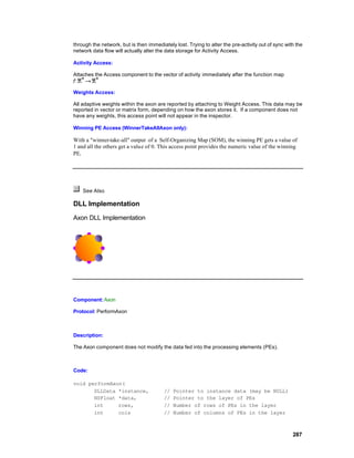
The BiasAxon component adds a bias term to each processing element (PE). The bias vector
contains the bias term for each PE and can be thought of as the Axon’s adaptable weights.
Code:
void performBiasAxon(
DLLData *instance, // Pointer to instance data (may be NULL)
NSFloat *data, // Pointer to the layer of PEs
int rows, // Number of rows of PEs in the layer
int cols // Number of columns of PEs in the layer
NSFloat *bias // Pointer to the layer's bias vector
)
{
int i, length=rows*cols;
for (i=0; i<length; i++)
data[i] += bias[i];
}
GaussianAxon DLL Implementation
288](https://image.slidesharecdn.com/neurosolutionshelp-090922003656-phpapp01/85/NeuroDimension-Neuro-Solutions-HELP-288-320.jpg)
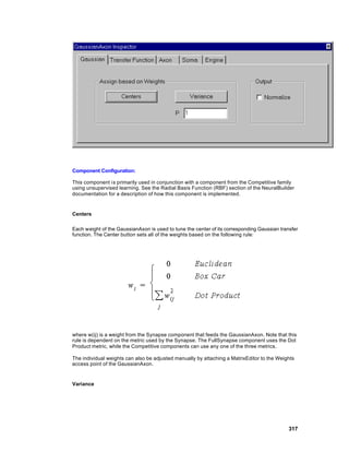
![Component: GaussianAxon
Protocol: PerformLinearAxon
Description:
The GaussianAxon applies a gaussian function to each neuron i n the layer. The bias vector
determines the center of the gaussian for each PE, and the beta term determines the width of the
gaussian for all PEs. The range of values for each neuron in the layer is between 0 and 1.
Code:
void performLinearAxon(
DLLData *instance, // Pointer to instance data (may be NULL)
NSFloat *data, // Pointer to the layer of PEs
int rows, // Number of rows of PEs in the layer
int cols // Number of columns of PEs in the layer
NSFloat *bias // Pointer to the layer's bias vector
NSFloat beta // Slope gain scalar, same for all PEs
)
{
int i, length=rows*cols;
for (i=0; i<length; i++) {
data[i] += bias[i];
data[i] = (NSFloat)exp(-beta*data[i]*data[i]);
}
}
LinearAxon DLL Implementation
Component: LinearAxon
Protocol: PerformLinearAxon
Description:
289](https://image.slidesharecdn.com/neurosolutionshelp-090922003656-phpapp01/85/NeuroDimension-Neuro-Solutions-HELP-289-320.jpg)
![The LinearAxon component adds to the functionality of the BiasAxon by adding a beta term that is
the same for all processing elements (PEs). This scalar specifies the slope of the linear transfer
function.
Code:
void performLinearAxon(
DLLData *instance, // Pointer to instance data (may be NULL)
NSFloat *data, // Pointer to the layer of PEs
int rows, // Number of rows of PEs in the layer
int cols // Number of columns of PEs in the layer
NSFloat *bias // Pointer to the layer's bias vector
NSFloat beta // Slope gain scalar, same for all PEs
)
{
int i, length=rows*cols;
for (i=0; i<length; i++)
data[i] = beta*data[i] + bias[i];
}
LinearSigmoidAxon DLL Implementation
Component: LinearSigmoidAxon
Protocol: PerformLinearAxon
Description:
The implementation for the LinearSigmoidAxon is the same as that of the LinearAxon except that
the transfer function is clipped at 0 and 1.
Code:
void performLinearAxon(
DLLData *instance, // Pointer to instance data (may be NULL)
NSFloat *data, // Pointer to the layer of PEs
int rows, // Number of rows of PEs in the layer
int cols // Number of columns of PEs in the layer
NSFloat *bias // Pointer to the layer's bias vector
290](https://image.slidesharecdn.com/neurosolutionshelp-090922003656-phpapp01/85/NeuroDimension-Neuro-Solutions-HELP-290-320.jpg)
![NSFloat beta // Slope gain scalar, same for all PEs
)
{
int i, length=rows*cols;
for (i=0; i<length; i++) {
data[i] = beta*data[i] + bias[i];
if (data[i] < 0.0f)
data[i] = 0.0f;
else
if (data[i] > 1.0f)
data[i] = 1.0f;
}
}
LinearTanhAxon DLL Implementation
Component: LinearTanhAxon
Protocol: PerformLinearAxon
Description:
The implementation for the LinearTanhAxon is the same as that of the LinearAxon except that the
transfer function is clipped at -1 and 1.
Code:
void performLinearAxon(
DLLData *instance, // Pointer to instance data (may be NULL)
NSFloat *data, // Pointer to the layer of PEs
int rows, // Number of rows of PEs in the layer
int cols // Number of columns of PEs in the layer
NSFloat *bias // Pointer to the layer's bias vector
NSFloat beta // Slope gain scalar, same for all PEs
)
{
int i, length=rows*cols;
for (i=0; i<length; i++) {
data[i] = beta*data[i] + bias[i];
291](https://image.slidesharecdn.com/neurosolutionshelp-090922003656-phpapp01/85/NeuroDimension-Neuro-Solutions-HELP-291-320.jpg)
![if (data[i] < -1.0f)
data[i] = -1.0f;
else
if (data[i] > 1.0f)
data[i] = 1.0f;
}
}
SigmoidAxon DLL Implementation
Component: SigmoidAxon
Protocol: PerformLinearAxon
Description:
The SigmoidAxon applies a scaled and biased sigmoid function to each neuron in the layer. The
range of values for each neuron in the layer is between 0 and 1.
Code:
void performLinearAxon(
DLLData *instance, // Pointer to instance data (may be NULL)
NSFloat *data, // Pointer to the layer of PEs
int rows, // Number of rows of PEs in the layer
int cols // Number of columns of PEs in the layer
NSFloat *bias // Pointer to the layer's bias vector
NSFloat beta // Slope gain scalar, same for all PEs
)
{
int i, length=rows*cols;
for (i=0; i<length; i++)
data[i] = 1.0f / (1.0f + (NSFloat)exp(-(beta*data[i] +
bias[i])));
}
SoftMaxAxon DLL Implementation
292](https://image.slidesharecdn.com/neurosolutionshelp-090922003656-phpapp01/85/NeuroDimension-Neuro-Solutions-HELP-292-320.jpg)
![Component: SoftMaxAxon
Protocol: PerformLinearAxon
Description:
The SoftMaxAxon is a component used to interpret the output of the neural net as a probability,
such that the sum of the outputs is equal to one. Unlike the WinnerTakeAllAxon, this component
outputs positive values for the non-maximum PEs. The beta term determines how hard or soft the
max function is. A high beta corresponds to a harder max; meaning that the PE with the highest
value is accentuated compared to the other PEs. The bias vector has no effect on this component.
The range of values for each neuron in the layer is between 0 and 1.
Code:
void performLinearAxon(
DLLData *instance, // Pointer to instance data (may be NULL)
NSFloat *data, // Pointer to the layer of PEs
int rows, // Number of rows of PEs in the layer
int cols // Number of columns of PEs in the layer
NSFloat *bias // Pointer to the layer's bias vector
NSFloat beta // Slope gain scalar, same for all PEs
)
{
int i, length=rows*cols;
NSFloat sum=(NSFloat)0.0;
for (i=0; i<length; i++) {
data[i] = beta*data[i];
sum += data[i] = (NSFloat)exp(data[i]);
}
for (i=0; i<length; i++)
data[i] /= sum;
}
TanhAxon DLL Implementation
293](https://image.slidesharecdn.com/neurosolutionshelp-090922003656-phpapp01/85/NeuroDimension-Neuro-Solutions-HELP-293-320.jpg)
![Component: TanhAxon
Protocol: PerformLinearAxon
Description:
The TanhAxon applies a scaled and biased hyperbolic tangent function to each neuron in the layer.
The range of values for each neuron in the layer is between -1 and 1.
Code:
void performLinearAxon(
DLLData *instance, // Pointer to instance data (may be NULL)
NSFloat *data, // Pointer to the layer of PEs
int rows, // Number of rows of PEs in the layer
int cols // Number of columns of PEs in the layer
NSFloat *bias // Pointer to the layer's bias vector
NSFloat beta // Slope gain scalar, same for all PEs
)
{
int i, length=rows*cols;
for (i=0; i<length; i++)
data[i] = (NSFloat)tanh(beta*data[i] + bias[i]);
}
ThresholdAxon DLL Implementation
Component: ThresholdAxon
Protocol: PerformBiasAxon
Description:
The ThresholdAxon component uses the bias term of each processing element (PE) as a
threshold. If the value of a given PE is less than or equal to its corresponding threshold, then this
value is set to -1. Otherwise, the PE’s value is set to 1.
294](https://image.slidesharecdn.com/neurosolutionshelp-090922003656-phpapp01/85/NeuroDimension-Neuro-Solutions-HELP-294-320.jpg)
![Code:
void performBiasAxon(
DLLData *instance, // Pointer to instance data (may be NULL)
NSFloat *data, // Pointer to the layer of PEs
int rows, // Number of rows of PEs in the layer
int cols // Number of columns of PEs in the layer
NSFloat *bias // Pointer to the layer's bias vector
)
{
int i, length=rows*cols;
for (i=0; i<length; i++) {
data[i] += bias[i];
data[i] = data[i] > 0? (NSFloat)1.0: (NSFloat)-1.0;
}
}
WinnerTakeAllAxon DLL Implementation
Component: WinnerTakeAllAxon
Protocol: PerformAxon
Description:
The WinnerTakeAllAxon component determines the processing element (PE) with the highest
value and declares it as the winner. It then sets the value of the winning PE to 1 and the rest to 0.
Code:
void performAxon(
DLLData *instance, // Pointer to instance data
NSFloat *data, // Pointer to the layer of PEs
int rows, // Number of rows of PEs in the layer
int cols // Number of columns of PEs in the layer
)
{
register int i, length=rows*cols, winner=0;
295](https://image.slidesharecdn.com/neurosolutionshelp-090922003656-phpapp01/85/NeuroDimension-Neuro-Solutions-HELP-295-320.jpg)
![for (i=1; i<length; i++)
if (data[i] > data[winner])
winner = i;
for (i=0; i<length; i++)
data[i] = (NSFloat)0.0;
data[winner] = (NSFloat)1.0;
}
Examples
Axon Example
Component: Axon
The Axon’s activation function is the identity map. It is normally used just as a storage unit. Recall
however, that all axons have a summing junction at their input and a node junction at their output.
The Axon will often be used purely to accumulate/distribute vectors of activity to/from other network
components.
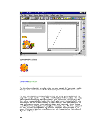
The figure below illustrates the output of an Axon with a ramp function as the input. The ramp in
this example provides a sweep of 100 points from [-1,1). Notice that the output is equal to the input
as expected. To experiment with this example, load the breadboard AxonExample.nsb.
296](https://image.slidesharecdn.com/neurosolutionshelp-090922003656-phpapp01/85/NeuroDimension-Neuro-Solutions-HELP-296-320.jpg)


![DLL Implementation
Macro Actions
DLL Implementation
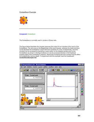
ContextAxon DLL Implementation
Component: ContextAxon
Protocol: PerformContextAxon
Description:
The ContextAxon integrates the activity received by each PE in the layer using an adaptable time
constant. Each PE within the data vector is computed by adding the product of the PE’s time
constant and the activity of the PE at the previous time step to the current activity. This sum is then
multiplied by a user-defined scaling factor.
Code:
void performContextAxon(
DLLData *instance, // Pointer to instance data (may be NULL)
NSFloat *data, // Pointer to the layer of PEs
int rows, // Number of rows of PEs in the layer
int cols // Number of columns of PEs in the layer
NSFloat *delayedData, // Pointer to a delayed PE layer
NSFloat *tau, // Pointer to a vector of time constants
NSFloat beta // Linear scaling factor (user-defined)
)
{
int i, length=rows*cols;
for (i=0; i<length; i++)
data[i] = beta * (data[i] + tau[i] * delayedData[i]);
}
GammaAxon DLL Implementation
332](https://image.slidesharecdn.com/neurosolutionshelp-090922003656-phpapp01/85/NeuroDimension-Neuro-Solutions-HELP-332-320.jpg)
![Component: GammaAxon
Protocol: PerformGammaAxon
Description:
The GammaAxon is a multi -channel tapped delay line with a Gamma memory structure. With a
straight tapped delay line (TDNNAxon), each memory tap (PE) within the data vector is computed
by simply copying the value from the previous tap of the delayedData vector. With the
GammaAxon, a given tap within data vector is computed by taking a fraction (gamma) of the value
from the previous tap of the delayedData vector and adding it with a fraction (1-gamma) of the
same tap. The first PE of each channel (tap[0]) is simply the channel’s input and is not modified.
Code:
void performGammaAxon(
DLLData *instance, // Pointer to instance data (may be NULL)
NSFloat *data, // Pointer to the layer of PEs
int rows, // Number of rows of PEs in the layer
int cols // Number of columns of PEs in the layer
NSFloat *delayedData, // Pointer to a delayed PE layer
int taps // Number of memory taps
NSFloat *gamma // Pointer to vector of gamma coefficients
)
{
register int i,j,k,length=rows*cols;
for (i=0; i<length; i++)
for (j=1; j<taps; j++) {
k = i + j*length;
data[k] = gamma[i]*delayedData[k-length] + (1-
gamma[i])*delayedData[k];
}
}
IntegratorAxon DLL Implementation
333](https://image.slidesharecdn.com/neurosolutionshelp-090922003656-phpapp01/85/NeuroDimension-Neuro-Solutions-HELP-333-320.jpg)
![Component: IntegratorAxon
Protocol: PerformContextAxon
Description:
The IntegratorAxon is very similar to the BackLaguarreAxon DLL Implementation, except that the
feedback connection is normalized. Each PE within the data vector is computed by adding the
product of the PE’s time constant and the activity of the PE at the previous time step to the product
of current activity times 1 minus the time constant. This sum is then multiplied by a user-defined
scaling factor.
Code:
void performContextAxon(
DLLData *instance, // Pointer to instance data (may be NULL)
NSFloat *data, // Pointer to the layer of PEs
int rows, // Number of rows of PEs in the layer
int cols // Number of columns of PEs in the layer
NSFloat *delayedData, // Pointer to a delayed PE layer
NSFloat *tau, // Pointer to a vector of time constants
NSFloat beta // Linear scaling factor (user-defined)
)
{
int i, length=rows*cols;
for (i=0; i<length; i++)
data[i] = (NSFloat)(beta * ((1.0-tau[i])*data[i] +
tau[i]*delayedData[i]));
}
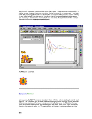
LaguarreAxon DLL Implementation
Component: LaguarreAxon
Protocol: PerformGammaAxon
334](https://image.slidesharecdn.com/neurosolutionshelp-090922003656-phpapp01/85/NeuroDimension-Neuro-Solutions-HELP-334-320.jpg)
![Description:
The LaguarreAxon is a multi -channel tapped delay line similar to the GammaAxon. The difference
is that this algorithm provides an orthogonal span of the memory space.
Code:
void performGammaAxon(
DLLData *instance, // Pointer to instance data (may be NULL)
NSFloat *data, // Pointer to the layer of PEs
int rows, // Number of rows of PEs in the layer
int cols // Number of columns of PEs in the layer
NSFloat *delayedData, // Pointer to a delayed PE layer
int taps // Number of memory taps
NSFloat *gamma // Pointer to vector of gamma coefficients
)
{
register int i,j,k,length=rows*cols;
for (i=0; i<length; i++) {
NSFloat gain = (NSFloat)pow(1-pow(gamma[i], 2), 0.5);
for (j=1; j<taps; j++) {
k = i + j*length;
data[k] = delayedData[k-length] +
gamma[i]*delayedData[k];
if (j==1)
data[k] *= gain;
else
data[k] -= gamma[i]*data[k-length];
}
}
}
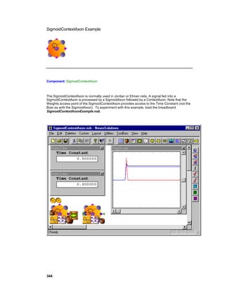
SigmoidContextAxon DLL Implementation
Component: SigmoidContextAxon
Protocol: PerformContextAxon
Description:
335](https://image.slidesharecdn.com/neurosolutionshelp-090922003656-phpapp01/85/NeuroDimension-Neuro-Solutions-HELP-335-320.jpg)
![The SigmoidContextAxon is very similar to the ContextAxon, except that the transfer function of
each PE is a sigmoid (i.e., saturates at 0 and 1) and the feedback is taken from this output.
Code:
void performContextAxon(
DLLData *instance, // Pointer to instance data (may be NULL)
NSFloat *data, // Pointer to the layer of PEs
int rows, // Number of rows of PEs in the layer
int cols // Number of columns of PEs in the layer
NSFloat *delayedData, // Pointer to a delayed PE layer
NSFloat *tau, // Pointer to a vector of time constants
NSFloat beta // Linear scaling factor (user-defined)
)
{
int i, length=rows*cols;
for (i=0; i<length; i++) {
data[i] = beta * (data[i] + tau[i] * delayedData[i]);
data[i] = (NSFloat)(1.0/(1.0+exp(-data[i])));
}
}
SigmoidIntegratorAxon DLL Implementation
Component: SigmoidIntegratorAxon
Protocol: PerformContextAxon
Description:
The SigmoidIntegratorAxon is very similar to the IntegratorAxon, except that the transfer function of
each PE is a sigmoid (i.e., saturates at 0 and 1) and the feedback is taken from this output.
Code:
void performContextAxon(
DLLData *instance, // Pointer to instance data (may be NULL)
NSFloat *data, // Pointer to the layer of PEs
int rows, // Number of rows of PEs in the layer
336](https://image.slidesharecdn.com/neurosolutionshelp-090922003656-phpapp01/85/NeuroDimension-Neuro-Solutions-HELP-336-320.jpg)
![int cols // Number of columns of PEs in the layer
NSFloat *delayedData, // Pointer to a delayed PE layer
NSFloat *tau, // Pointer to a vector of time constants
NSFloat beta // Linear scaling factor (user-defined)
)
{
int i, length=rows*cols;
for (i=0; i<length; i++) {
data[i] = beta * ((1-tau[i])*data[i] +
tau[i]*delayedData[i]);
data[i] = 1/(1+(NSFloat)exp(-data[i]));
}
}
TanhContextAxon DLL Implementation
Component: TanhContextAxon
Protocol: PerformContextAxon
Description:
The TanhContextAxon is very similar to the ContextAxon, except that the transfer function of each
PE is a hyperbolic tangent (i.e., saturates at -1 and 1) and the feedback is taken from this output.
Code:
void performContextAxon(
DLLData *instance, // Pointer to instance data (may be NULL)
NSFloat *data, // Pointer to the layer of PEs
int rows, // Number of rows of PEs in the layer
int cols // Number of columns of PEs in the layer
NSFloat *delayedData, // Pointer to a delayed PE layer
NSFloat *tau, // Pointer to a vector of time constants
NSFloat beta // Linear scaling factor (user-defined)
)
{
int i, length=rows*cols;
for (i=0; i<length; i++)
337](https://image.slidesharecdn.com/neurosolutionshelp-090922003656-phpapp01/85/NeuroDimension-Neuro-Solutions-HELP-337-320.jpg)
![data[i] = (NSFloat)tanh(beta * (data[i] + tau[i] *
delayedData[i]));
}
TanhIntegratorAxon DLL Implementation
Component: TanhIntegratorAxon
Protocol: PerformContextAxon
Description:
The TanhIntegratorAxon is very similar to the IntegratorAxon, except that the transfer function of
each PE is a hyperbolic tangent (i.e., saturates at -1 and 1) and the feedback is taken from this
output.
Code:
void performContextAxon(
DLLData *instance, // Pointer to instance data (may be NULL)
NSFloat *data, // Pointer to the layer of PEs
int rows, // Number of rows of PEs in the layer
int cols // Number of columns of PEs in the layer
NSFloat *delayedData, // Pointer to a delayed PE layer
NSFloat *tau, // Pointer to a vector of time constants
NSFloat beta // Linear scaling factor (user-defined)
)
{
for (i=0; i<length; i++)
data[i] = (NSFloat)tanh(beta * ((1-tau[i])*data[i] +
tau[i]*delayedData[i]));
}
TDNNAxon DLL Implementation
338](https://image.slidesharecdn.com/neurosolutionshelp-090922003656-phpapp01/85/NeuroDimension-Neuro-Solutions-HELP-338-320.jpg)
![Component: TDNNAxon
Protocol: PerformTDNNAxon
Description:
The TDNNAxon is a multi -channel tapped delay line memory structure. For each memory tap (PE)
within the data vector, the value is copied from the previous tap of the delayedData vector. The first
PE of each channel (tap[0]) is simply the channel’s input and is not modified.
Code:
void performTDNNAxon(
DLLData *instance, // Pointer to instance data (may be NULL)
NSFloat *data, // Pointer to the layer of PEs
int rows, // Number of rows of PEs in the layer
int cols // Number of columns of PEs in the layer
NSFloat *delayedData, // Pointer to a delayed PE layer
int taps // Number of memory taps
)
{
register int i,j,k,length=rows*cols;
for (i=0; i<length; i++)
for (j=1; j<taps; j++) {
k = i + j*length;
data[k] = delayedData[k-length];
}
}
Examples
IntegratorAxon Example
Component: IntegratorAxon
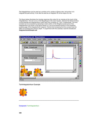
339](https://image.slidesharecdn.com/neurosolutionshelp-090922003656-phpapp01/85/NeuroDimension-Neuro-Solutions-HELP-339-320.jpg)


![void performFullSynapse(
DLLData *instance, // Pointer to instance data (may be NULL)
NSFloat *input, // Pointer to the input layer of PEs
int inRows, // Number of rows of PEs in the input layer
int inCols, // Number of columns of PEs in the input layer
NSFloat *output, // Pointer to the output layer
int outRows, // Number of rows of PEs in the output layer
int outCols // Number of columns of PEs in the output layer
NSFloat *weights // Pointer to the fully-connected weight matrix
)
{
int i, j,
inCount=inRows*inCols,
outCount=outRows*outCols;
for (i=0; i<outCount; i++)
for (j=0; j<inCount; j++)
output[i] += W(i,j)*input[j];
}
Synapse DLL Implementation
Component: Synapse
Protocol: PerformSynapse
Description:
The Synapse component simply takes each PE from the Axon feeding the Synapse’s input and
adds its activity to the corresponding PE of the Axon at the Synapse’s output. The delay between
the input and output is defined by the user within the Synapse Inspector (see Synapse Family).
Note that the activity is accumulated at the output for the case of a summing junction (i.e.,
connection that is fed by multiple Synapses) at the output Axon. Also note that if there is a different
number of input PEs than output PEs, then the extra ones are ignored.
Code:
void performSynapse(
DLLData *instance, // Pointer to instance data (may be NULL)
NSFloat *input, // Pointer to the input layer of PEs
int inRows, // Number of rows of PEs in the input layer
366](https://image.slidesharecdn.com/neurosolutionshelp-090922003656-phpapp01/85/NeuroDimension-Neuro-Solutions-HELP-366-320.jpg)
![int inCols, // Number of columns of PEs in the input layer
NSFloat *output, // Pointer to the output layer
int outRows, // Number of rows of PEs in the output layer
int outCols // Number of columns of PEs in the output layer
)
{
int i,
inCount=inRows*inCols,
outCount=outRows*outCols,
count = inCount<outCount? inCount: outCount;
for (i=0; i<count; i++)
output[i] += input[i];
}
Drag and Drop
Synapse Family Drag and Drop
Synapses are base components on the breadboard. This means that they must be dropped directly
onto an empty breadboard location.
See Also
Inspectors
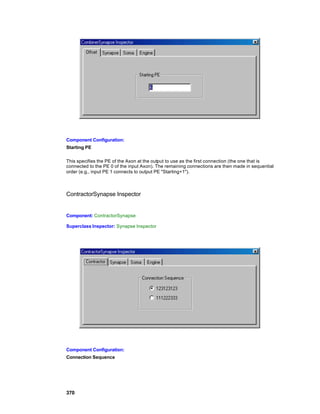
ArbitrarySynapse Inspector
Component: ArbitrarySynapse
Superclass Inspector: Synapse Inspector
367](https://image.slidesharecdn.com/neurosolutionshelp-090922003656-phpapp01/85/NeuroDimension-Neuro-Solutions-HELP-367-320.jpg)


![}
BackBiasAxon DLL Implementation
Component: BackBiasAxon
Protocol: PerformBackBiasAxon
Description:
Since the partial of the BiasAxon’s cost with respect to its activity is 1, the sensitivity vector is not
modified. The partial of the BiasAxon’s cost with respect to its weight vector is used to compute the
gradient vector. This vector is simply an accumulation of the error.
Code:
void performBackBiasAxon(
DLLData *instance, // Pointer to instance data
DLLData *dualInstance, // Pointer to forward axon’s instance data
NSFloat *data, // Pointer to the layer of PEs
int rows, // Number of rows of PEs in the layer
int cols, // Number of columns of PEs in the layer
NSFloat *error // Pointer to the sensitivity vector
NSFloat *gradient // Pointer to the bias gradient vector
)
{
int i, length=rows*cols;
if (gradient)
for (i=0; i<length; i++)
gradient[i] += error[i];
}
BackLinearAxon DLL Implementation
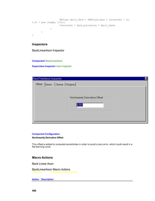
394](https://image.slidesharecdn.com/neurosolutionshelp-090922003656-phpapp01/85/NeuroDimension-Neuro-Solutions-HELP-394-320.jpg)
![Component: BackLinearAxon
Protocol: PerformBackLinearAxon
Description:
The partial of the LinearAxon’s cost with respect to its activity is the sensitivity from the previous
layer times beta. The partial of the LinearAxon’s cost with respect to its weight vector is used to
compute the gradient vector. As with the BiasAxon, this vector is simply an accumulation of the
error.
Code:
void performBackLinearAxon(
DLLData *instance, // Pointer to instance data
DLLData *dualInstance, // Pointer to forward axon’s instance data
NSFloat *data, // Pointer to the layer of PEs
int rows, // Number of rows of PEs in the layer
int cols, // Number of columns of PEs in the layer
NSFloat *error // Pointer to the sensitivity vector
NSFloat *gradient // Pointer to the bias gradient vector
NSFloat beta // Slope gain scalar, same for all PEs
)
{
int i, length=rows*cols;
for (i=0; i<length; i++) {
error[i] *= beta;
if (gradient)
gradient[i] += error[i];
}
}
BackSigmoidAxon DLL Implementation
Component: BackSigmoidAxon
Protocol: PerformBackLinearAxon
Description:
395](https://image.slidesharecdn.com/neurosolutionshelp-090922003656-phpapp01/85/NeuroDimension-Neuro-Solutions-HELP-395-320.jpg)
![The partial of the SigmoidAxon’s cost with respect to its activity is used to compute the sensitivity
vector. The partial of the SigmoidAxon’s cost with respect to its weight vector is used to compute
the gradient vector. As with the BiasAxon, this vector is simply an accumulation of the error.
Code:
void performBackLinearAxon(
DLLData *instance, // Pointer to instance data
DLLData *dualInstance, // Pointer to forward axon’s instance data
NSFloat *data, // Pointer to the layer of PEs
int rows, // Number of rows of PEs in the layer
int cols, // Number of columns of PEs in the layer
NSFloat *error // Pointer to the sensitivity vector
NSFloat *gradient // Pointer to the bias gradient vector
NSFloat beta // Slope gain scalar, same for all PEs
)
{
int i, length=rows*cols;
for (i=0; i<length; i++) {
error[i] *= beta*(data[i]*(1.0f-data[i]) + 0.1f);
if (gradient)
gradient[i] += error[i];
}
}
BackTanhAxon DLL Implementation
Component: BackTanhAxon
Protocol: PerformBackLinearAxon
Description:
The partial of the TanhAxon’s cost with respect to its activity is used to compute the sensitivity
vector. The partial of the TanhAxon’s cost with respect to its weight vector is used to compute the
gradient vector. As with the BiasAxon, this vector is simply an accumulation of the error.
Code:
void performBackLinearAxon(
DLLData *instance, // Pointer to instance data
396](https://image.slidesharecdn.com/neurosolutionshelp-090922003656-phpapp01/85/NeuroDimension-Neuro-Solutions-HELP-396-320.jpg)
![DLLData *dualInstance, // Pointer to forward axon’s instance data
NSFloat *data, // Pointer to the layer of PEs
int rows, // Number of rows of PEs in the layer
int cols, // Number of columns of PEs in the layer
NSFloat *error // Pointer to the sensitivity vector
NSFloat *gradient // Pointer to the bias gradient vector
NSFloat beta // Slope gain scalar, same for all PEs
)
{
int i, length=rows*cols;
for (i=0; i<length; i++) {
error[i] *= beta*(1.0f - data[i]*data[i] + 0.1f);
if (gradient)
gradient[i] += error[i];
}
}
BackBellFuzzyAxon DLL Implementation
Component: BackBellFuzzyAxon
Protocol: PerformBackFuzzyAxon
Description:
The BellFuzzyAxon has three parameters for each membership function. This function computes
the partial of each of those parameters with respect to the input value corresponding to the winning
membership function.
Code:
void performBackFuzzyAxon(
DLLData *instance, // Pointer to instance data (may be
NULL)
DLLData *dualInstance,// Pointer to forward axon’s instance
data
// (may be NULL)
NSFloat *data, // Pointer to the layer of
processing
// elements (PEs)
int rows, // Number of rows of PEs in the
layer
int cols, // Number of columns of PEs in
397](https://image.slidesharecdn.com/neurosolutionshelp-090922003656-phpapp01/85/NeuroDimension-Neuro-Solutions-HELP-397-320.jpg)


![DLL Implementation
BackContextAxon DLL Implementation
Component: BackContextAxon
Protocol: PerformBackContextAxon
Description:
The gradient information is computed to update the time constants and the sensitivity vector is
computed for the backpropagation.
Code:
void performBackContextAxon(
DLLData *instance, // Pointer to instance data (may be NULL)
DLLData *dualInstance, // Pointer to forward axon’s instance data
NSFloat *error, // Pointer to the current sensitivity
vector
int rows, // Number of rows of PEs in the layer
int cols, // Number of columns of PEs in the layer
NSFloat *delayedError, // Pointer to the delayed error vector
NSFloat *data, // Pointer to the layer of PEs
NSFloat *tau, // Pointer to a vector of time constants
NSFloat beta, // Linear scaling factor (user-defined)
NSFloat *gradient // Pointer to the tau gradient vector
)
{
int i, length=rows*cols;
for (i=0; i<length; i++) {
error[i] = beta*(data[i] + tau[i]*delayedError[i]);
if (gradient)
gradient[i] += delayedError[i]*beta*data[i];
}
}
BackGammaAxon DLL Implementation
409](https://image.slidesharecdn.com/neurosolutionshelp-090922003656-phpapp01/85/NeuroDimension-Neuro-Solutions-HELP-409-320.jpg)
![Component: BackGammaAxon
Protocol: PerformBackGammaAxon
Description:
The gradient information is computed to update the gamma coefficients and the sensitivity vector is
computed for the backpropagation.
Code:
void performBackGammaAxon(
DLLData *instance, // Pointer to instance data (may be NULL)
DLLData *dualInstance, // Pointer to forward axon’s instance data
NSFloat *error, // Pointer to the current sensitivity
vector
int rows, // Number of rows of PEs in the layer
int cols, // Number of columns of PEs in the layer
NSFloat *delayedError, // Pointer to the delayed error vector
int taps, // Number of memory taps (user-defined)
NSFloat *data // Pointer to the layers of (PEs)
NSFloat *gamma, // Pointer to vector of gamma coefficients
NSFloat *gradient // Pointer to the gamma gradient vector
)
{
register int i,j,k,length=rows*cols;
for (i=0; i<length; i++)
for (j=1; j<taps; j++) {
k = i + j*length;
error[k-length] += gamma[i]*delayedError[k];
error[k] += (1.0f-gamma[i])*delayedError[k];
if (gradient)
gradient[i] += delayedError[k]*(data[k-
length]-data[k]);
}
}
BackIntegratorAxon DLL Implementation
410](https://image.slidesharecdn.com/neurosolutionshelp-090922003656-phpapp01/85/NeuroDimension-Neuro-Solutions-HELP-410-320.jpg)
![Component: BackIntegratorAxon
Protocol: PerformBackContextAxon
Description:
The gradient information is computed to update th e time constants and the sensitivity vector is
computed for the backpropagation.
Code:
void performBackContextAxon(
DLLData *instance, // Pointer to instance data (may be NULL)
DLLData *dualInstance, // Pointer to forward axon’s instance data
NSFloat *error, // Pointer to the current sensitivity
vector
int rows, // Number of rows of PEs in the layer
int cols, // Number of columns of PEs in the layer
NSFloat *delayedError, // Pointer to the delayed error vector
NSFloat *data, // Pointer to the layer of PEs
NSFloat *tau, // Pointer to a vector of time constants
NSFloat beta, // Linear scaling factor (user-defined)
NSFloat *gradient // Pointer to the tau gradient vector
)
{
int i, length=rows*cols;
for (i=0; i<length; i++) {
error[i] = beta*((1.0f-tau[i])*data[i] +
tau[i]*delayedError[i]);
if (gradient)
gradient[i] += delayedError[i]*beta*data[i];
}
}
BackLaguarreAxon DLL Implementation
411](https://image.slidesharecdn.com/neurosolutionshelp-090922003656-phpapp01/85/NeuroDimension-Neuro-Solutions-HELP-411-320.jpg)
![Component: BackLaguarreAxon
Protocol: PerformBackGammaAxon DLL Protocol
Description:
The gradient information is computed to update the gamma coefficients and the sensitivity vector is
computed for the backpropagation.
Code:
void performBackGammaAxon(
DLLData *instance, // Pointer to instance data (may be NULL)
DLLData *dualInstance, // Pointer to forward axon’s instance data
NSFloat *error, // Pointer to the current sensitivity
vector
int rows, // Number of rows of PEs in the layer
int cols, // Number of columns of PEs in the layer
NSFloat *delayedError, // Pointer to the delayed error vector
int taps, // Number of memory taps (user-defined)
NSFloat *data // Pointer to the layers of (PEs)
NSFloat *gamma, // Pointer to vector of gamma coefficients
NSFloat *gradient // Pointer to the gamma gradient vector
)
{
register int i,j,k,length=rows*cols;
NSFloat gain;
for (i=0; i<length; i++) {
gain = (NSFloat)pow(1-pow(gamma[i], 2.0f), 0.5f);
for (j=1; j<taps; j++) {
k = i + j*length;
error[k-length] += delayedError[k];
error[k] += gamma[i]*delayedError[k];
if (gradient)
gradient[i] += delayedError[k]*data[k];
if (j==1)
error[k] *= gain;
else {
error[k-length] -= gamma[i]*error[k];
if (gradient)
gradient[i] -= error[k]*data[k-length];
}
}
}
}
412](https://image.slidesharecdn.com/neurosolutionshelp-090922003656-phpapp01/85/NeuroDimension-Neuro-Solutions-HELP-412-320.jpg)
![BackSigmoidContextAxon DLL Implementation
Component: BackSigmoidContextAxon
Protocol: PerformBackContextAxon
Description:
The gradient information is computed to update the time constants and the sensitivity vector is
computed for the backpropagation.
Code:
void performBackContextAxon(
DLLData *instance, // Pointer to instance data (may be NULL)
DLLData *dualInstance, // Pointer to forward axon’s instance data
NSFloat *error, // Pointer to the current sensitivity
vector
int rows, // Number of rows of PEs in the layer
int cols, // Number of columns of PEs in the layer
NSFloat *delayedError, // Pointer to the delayed error vector
NSFloat *data, // Pointer to the layer of PEs
NSFloat *tau, // Pointer to a vector of time constants
NSFloat beta, // Linear scaling factor (user-defined)
NSFloat *gradient // Pointer to the tau gradient vector
)
{
int i, length=rows*cols;
for (i=0; i<length; i++) {
error[i] *= data[i]*(1.0f-data[i]) + 0.1f;
error[i] = beta*(data[i] + tau[i]*delayedError[i]);
if (gradient)
gradient[i] += delayedError[i]*beta*data[i];
}
}
BackSigmoidIntegratorAxon DLL Implementation
413](https://image.slidesharecdn.com/neurosolutionshelp-090922003656-phpapp01/85/NeuroDimension-Neuro-Solutions-HELP-413-320.jpg)
![Component: BackSigmoidIntegratorAxon
Protocol: PerformBackContextAxon
Description:
The gradient information is computed to update the time constants and the sensitivity vector is
computed for the backpropagation.
Code:
void performBackContextAxon(
DLLData *instance, // Pointer to instance data (may be NULL)
DLLData *dualInstance, // Pointer to forward axon’s instance data
NSFloat *error, // Pointer to the current sensitivity
vector
int rows, // Number of rows of PEs in the layer
int cols, // Number of columns of PEs in the layer
NSFloat *delayedError, // Pointer to the delayed error vector
NSFloat *data, // Pointer to the layer of PEs
NSFloat *tau, // Pointer to a vector of time constants
NSFloat beta, // Linear scaling factor (user-defined)
NSFloat *gradient // Pointer to the tau gradient vector
)
{
int i, length=rows*cols;
for (i=0; i<length; i++) {
error[i] *= data[i]*(1.0f-data[i]) + 0.1f;
error[i] = beta*((1.0f-tau[i])*data[i] +
tau[i]*delayedError[i]);
if (gradient)
gradient[i] += delayedError[i]*beta*data[i];
}
}
BackTanhContextAxon DLL Implementation
414](https://image.slidesharecdn.com/neurosolutionshelp-090922003656-phpapp01/85/NeuroDimension-Neuro-Solutions-HELP-414-320.jpg)
![Component: BackTanhContextAxon
Protocol: PerformBackContextAxon
Description:
The gradient information is computed to update the time constants and the sensitivity vector is
computed for the backpropagation.
Code:
void performBackContextAxon(
DLLData *instance, // Pointer to instance data (may be NULL)
DLLData *dualInstance, // Pointer to forward axon’s instance data
NSFloat *error, // Pointer to the current sensitivity
vector
int rows, // Number of rows of PEs in the layer
int cols, // Number of columns of PEs in the layer
NSFloat *delayedError, // Pointer to the delayed error vector
NSFloat *data, // Pointer to the layer of PEs
NSFloat *tau, // Pointer to a vector of time constants
NSFloat beta, // Linear scaling factor (user-defined)
NSFloat *gradient // Pointer to the tau gradient vector
)
{
int i, length=rows*cols;
for (i=0; i<length; i++) {
error[i] *= 1.0f - data[i]*data[i] + 0.1f;
error[i] = beta*(data[i] + tau[i]*delayedError[i]);
if (gradient)
gradient[i] += delayedError[i]*beta*data[i];
}
}
BackTanhIntegratorAxon DLL Implementation
Component: BackTanhIntegratorAxon
415](https://image.slidesharecdn.com/neurosolutionshelp-090922003656-phpapp01/85/NeuroDimension-Neuro-Solutions-HELP-415-320.jpg)
![Protocol: PerformBackContextAxon
Description:
The gradient information is computed to update the time constants and the sensitivity vector is
computed for the backpropagation.
Code:
void performBackContextAxon(
DLLData *instance, // Pointer to instance data (may be NULL)
DLLData *dualInstance, // Pointer to forward axon’s instance data
NSFloat *error, // Pointer to the current sensitivity
vector
int rows, // Number of rows of PEs in the layer
int cols, // Number of columns of PEs in the layer
NSFloat *delayedError, // Pointer to the delayed error vector
NSFloat *data, // Pointer to the layer of PEs
NSFloat *tau, // Pointer to a vector of time constants
NSFloat beta, // Linear scaling factor (user-defined)
NSFloat *gradient // Pointer to the tau gradient vector
)
{
int i, length=rows*cols;
for (i=0; i<length; i++) {
error[i] *= 1.0f - error[i]*error[i] + 0.1f;
error[i] = beta*((1.0f-tau[i])*error[i] +
tau[i]*delayedError[i]);
if (gradient)
gradient[i] += delayedError[i]*beta*data[i];
}
}
BackTDNNAxon DLL Implementation
Component: BackTDNNAxon
Protocol: PerformBackTDNNAxon
Description:
416](https://image.slidesharecdn.com/neurosolutionshelp-090922003656-phpapp01/85/NeuroDimension-Neuro-Solutions-HELP-416-320.jpg)
![Since the TDNNAxon has no adaptable weights, there is no gradient information to compute. The
sensitivity vector is computed by taking the backpropagated error from each PE and adding the
delayedError from the next tap.
Code:
void performBackTDNNAxon(
DLLData *instance, // Pointer to instance data (may be NULL)
DLLData *dualInstance, // Pointer to forward axon’s instance data
NSFloat *error, // Pointer to the current sensitivity
vector
int rows, // Number of rows of PEs in the layer
int cols, // Number of columns of PEs in the layer
NSFloat *delayedError, // Pointer to the delayed error vector
int taps, // Number of memory taps (user-defined)
NSFloat *data // Pointer to the layers of (PEs)
)
{
register int i,j,k,length=rows*cols;
for (i=0; i<length; i++)
for (j=1; j<taps; j++) {
k = i + j*length;
error[k-length] += delayedError[k];
}
}
BackSynapse Family
BackArbitrarySynapse
Family: BackSynapse Family
Superclass: BackSynapse
Activation Dual: ArbitrarySynapse
Sensitivity Function and Gradient Function:
There is no pre-specified map for the ArbitrarySynapse. This component will backpropagate the
sensitivities and gradients for any user defined connections within its dual component.
417](https://image.slidesharecdn.com/neurosolutionshelp-090922003656-phpapp01/85/NeuroDimension-Neuro-Solutions-HELP-417-320.jpg)

![Protocol: PerformBackFullSynapse
Description:
The gradient of the weight going from the jth PE of the input BackAxon to the ith PE of the output
BackAxon is the product of the error at the ith PE of the input BackAxon and the activity of the jth
PE of the output BackAxon’s activation dual component.
The error at the ith PE of the output BackAxon is the sum of the products of each weight connected
to that PE and the corresponding error at the input BackAxon. Note that the input and output are
reversed from the activation dual (i.e., the Synapse).
Code:
void performBackFullSynapse(
DLLData *instance, // Pointer to instance data (may be NULL)
DLLData *dualInstance, // Pointer to forward axon’s instance data
NSFloat *errorIn, // Pointer to the input error layer of PEs
int inRows, // Number of rows of PEs in the input layer
int inCols, // Number of columns of PEs at the input
NSFloat *errorOut, // Pointer to the output error layer
int outRows, // Number of rows of PEs in the output
layer
int outCols, // Number of columns of PEs at the output
NSFloat *input // Pointer to output PEs of forward synapse
NSFloat *weights, // Pointer to fully-connected weight matrix
NSFloat *gradients // Pointer to the weight gradient matrix
)
{
int i, j,
inCount=inRows*inCols,
outCount=outRows*outCols;
for (i=0; i<outCount; i++)
for (j=0; j<inCount; j++) {
errorOut[i] += W(j,i)*errorIn[j];
if (gradients)
Wg(j,i) += errorIn[j]*input[i];
}
}
BackSynapse DLL Implementation
420](https://image.slidesharecdn.com/neurosolutionshelp-090922003656-phpapp01/85/NeuroDimension-Neuro-Solutions-HELP-420-320.jpg)
![Component: BackSynapse
Protocol: PerformBackSynapse
Description:
Since the Synapse component has no adaptable weights, there is no gradient information
computed. The sensitivity vector is computed by taking the error from the previous backprop layer
and adding it to the error at the next backprop layer. Note that the error is accumulated at the
output for the case of a splitting node (i.e., connection that feeds multiple Synapses) at the Axon
that feeds the activation dual component (i.e., the Synapse).
The delay between the output and input is defined by the user within the inspector of the activation
dual (see Back Synapse Family). Note that the input and output are reversed from the activation
dual (i.e., the Synapse).
Code:
void performBackSynapse(
DLLData *instance, // Pointer to instance data (may be NULL)
DLLData *dualInstance, // Pointer to forward axon’s instance data
NSFloat *errorIn, // Pointer to the input error layer of PEs
int inRows, // Number of rows of PEs in the input layer
int inCols, // Number of columns of PEs at the input
NSFloat *errorOut, // Pointer to the output error layer
int outRows, // Number of rows of PEs in the output
layer
int outCols, // Number of columns of PEs at the output
NSFloat *input // Pointer to output PEs of forward synapse
)
{
int i,
inCount=inRows*inCols,
outCount=outRows*outCols,
count=inCount<outCount? inCount: outCount;
for (i=0; i<count; i++)
errorOut[i] += errorIn[i];
}
Drag and Drop
Backprop Family Drag and Drop
Each member of the Backprop family was custom developed to perform backpropagation for a
component in the Activation family. There is a one-to-one association between members of the
Backprop family and the adaptive Activation components. The Activation component associated
with any Backprop member will be referred to as its Activation dual. Each member of the
Backprop family must be dropped directly on its activation dual, or a subclass of its dual.
421](https://image.slidesharecdn.com/neurosolutionshelp-090922003656-phpapp01/85/NeuroDimension-Neuro-Solutions-HELP-421-320.jpg)

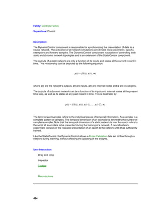
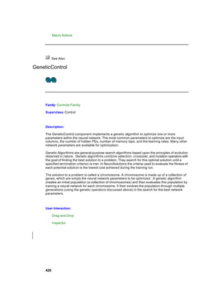


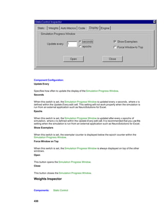

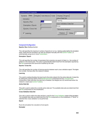

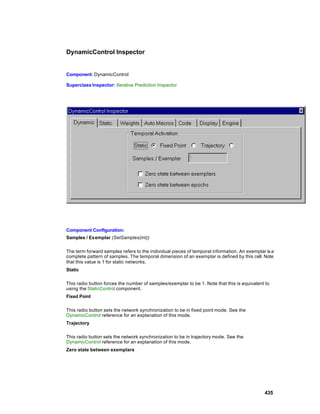
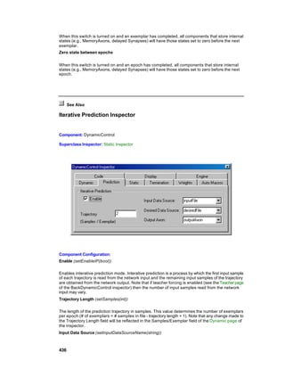


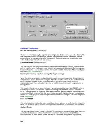

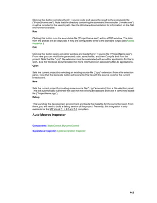


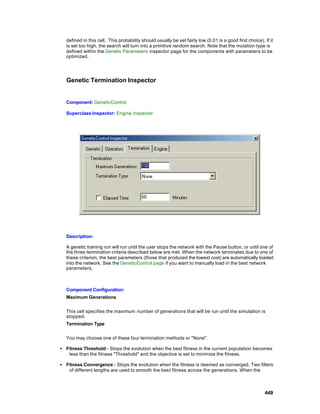


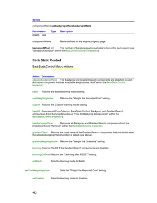


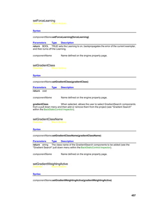

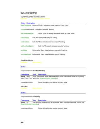

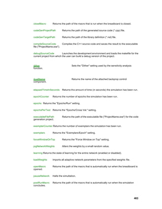


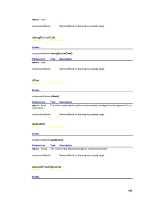

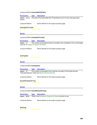

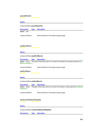

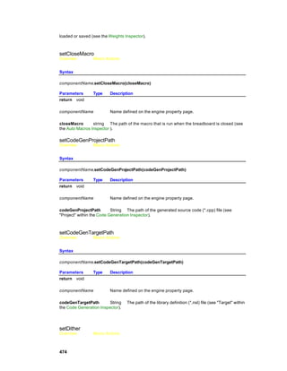


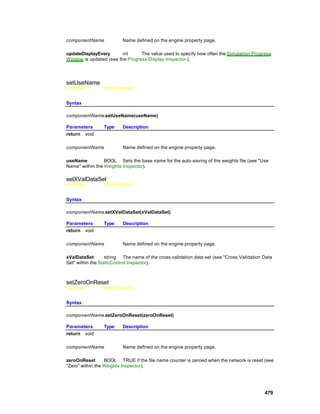

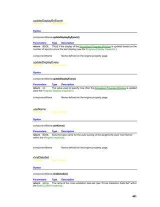

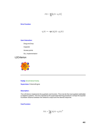
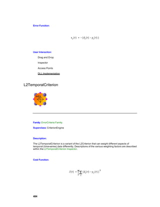
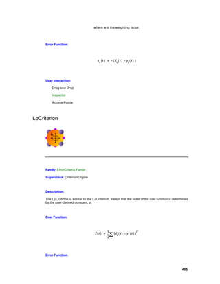
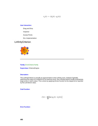


![int rows, // Number of rows of PEs in the layer
int cols, // Number of columns of PEs in the layer
NSFloat *output, // Pointer to output layer of the network
NSFloat *desired // Pointer to desired output vector
)
{
int i,length=rows*cols;
NSFloat cost=0.0f;
for (i=0; i<length; i++) {
costDerivative[i] = desired[i] - output[i] >= 0? (NSFloat)-
1.0 : (NSFloat)1.0;
cost += (NSFloat)fabs(desired[i] - output[i]);
}
return cost;
}
L2Criterion DLL Implementation
Component: L2Criterion
Protocol: PerformCriterion
Description:
The L2CriterionEngine implements the quadratic cost function. The error reported to the supervised
learning procedure (costDerivative) is simply the squared Euclidean distance between the net
work's output and the desired response, for each output PE. The cost returned is the accumulation
of the squared error, for all output PEs.
Code:
NSFloat performCriterion(
DLLData *instance, // Pointer to instance data (may be NULL)
NSFloat *costDerivative, // Pointer to output sensitivity vector
int rows, // Number of rows of PEs in the layer
int cols, // Number of columns of PEs in the layer
NSFloat *output, // Pointer to output layer of the network
NSFloat *desired // Pointer to desired output vector
)
{
490](https://image.slidesharecdn.com/neurosolutionshelp-090922003656-phpapp01/85/NeuroDimension-Neuro-Solutions-HELP-490-320.jpg)
![int i,length=rows*cols;
NSFloat cost=0.0f;
for (i=0; i<length; i++) {
costDerivative[i] = desired[i] - output[i];
cost += costDerivative[i]*costDerivative[i];
}
return cost;
}
LinfinityCriterion DLL Implementation
Component: LinfinityCriterion
Protocol: PerformCriterion
Description:
The LinfinityCriterionEngine implements an approximation to the Linfinity norm cost function. The
error reported to the supervised learning procedure (costDerivative) is simply the hyperbolic
tangent of the difference between the network's output and desired response, for each output PE.
This results in a local emphasis on large errors. The cost returned is the accumulation of the error,
for all output PEs.
Code:
NSFloat performCriterion(
DLLData *instance, // Pointer to instance data (may be NULL)
NSFloat *costDerivative, // Pointer to output sensitivity vector
int rows, // Number of rows of PEs in the layer
int cols, // Number of columns of PEs in the layer
NSFloat *output, // Pointer to output layer of the network
NSFloat *desired // Pointer to desired output vector
)
{
int i,length=rows*cols;
NSFloat cost=0.0f;
for (i=0; i<length; i++) {
costDerivative[i] = (NSFloat)tan(desired[i] - output[i]);
cost += (NSFloat)fabs(costDerivative[i]);
491](https://image.slidesharecdn.com/neurosolutionshelp-090922003656-phpapp01/85/NeuroDimension-Neuro-Solutions-HELP-491-320.jpg)
![}
return cost;
}
DeltaBarDelta DLL Implementation
Component: DeltaBarDelta
Protocol: PerformDeltaBarDelta
Description:
The implementation of the DeltaBarDelta component computes the step size for each of the
weights based on the gradient from the backprop component, a smoothed version of the gradient
(smoothedGradient), and three constants (beta, kappa, and zeta) defined by the user within the
DeltaBarDelta inspector. This function is responsible for updating both the step and
smoothedGradient vectors. Note that the updating of the weights uses the standard Momentum
rule, and is performed by the component itself.
Code:
void performDeltaBarDelta(
DLLData *instance, // Pointer to instance data
NSFloat *step, // Pointer to vector of learning rates
int length, // Length of learning rate vector
NSFloat *smoothedGradient, // Smoothed gradient vector
NSFloat *gradient, // Gradient vector from backprop comp.
NSFloat beta, // Multiplicative constant
NSFloat kappa, // Additive constant
NSFloat zeta // Smoothing factor
)
{
register int i;
for (i=0; i<length; i++) {
if (smoothedGradient[i]*gradient[i] > 0)
step[i] += kappa;
else
if (smoothedGradient[i]*gradient[i] < 0)
step[i] -= beta*step[i];
smoothedGradient[i] = (1-zeta)*gradient[i] +
zeta*smoothedGradient[i];
}
}
492](https://image.slidesharecdn.com/neurosolutionshelp-090922003656-phpapp01/85/NeuroDimension-Neuro-Solutions-HELP-492-320.jpg)


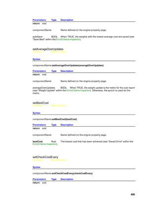

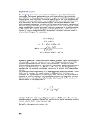
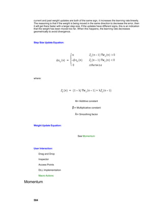


![See Also
DLL Implementation
Momentum DLL Implementation
Component: Momentum
Protocol: PerformMomentum
Description:
The implementation of the Momentum component is similar to that of the Step component, except
that there is the addition of a momentum term and a vector containing the previous weight change
(delta). The delta for a given weight is computed by taking product of the momentum rate and the
weight’s previous delta and adding it to the product of the step size and the weight’s gradient. Note
that this function is responsible for updating the delta vector as well as the weights vector.
Code:
void performMomentum(
DLLData *instance, // Pointer to instance data
NSFloat *weights, // Pointer to the vector of weights
int length, // Length of the weight vector
NSFloat *gradient, // Pointer to vector of gradients
NSFloat *step, // Pointer to the learning rate/s
BOOL individual // Indicates whether there is one learning
rate
// for all weights (FALSE), or each weight has
// its own learning rate (TRUE)
NSFloat *delta, // Last weight Update
NSFloat momentum // Momentum rate for all weights
)
{
register int i;
for (i=0; i<length; i++)
weights[i] += delta[i] = momentum*delta[i] +
step[individual?i:0]*gradient[i];
}
509](https://image.slidesharecdn.com/neurosolutionshelp-090922003656-phpapp01/85/NeuroDimension-Neuro-Solutions-HELP-509-320.jpg)
![Quickprop DLL Implementation
Component: Quickprop
Protocol: PerformQuickprop
Description:
The implementation of the Quickprop component is similar to that of the Momentum component,
except that the momentum rate is unique to each weight. This vector is computed from the gradient
information from the previous (lastGradient) and current (gradient) weight updates. The absolute
value of the individual momentum terms is limited by the defaultMomentum defined by the user
within the inspector. Note that this vector could have been allocated as local storage, but it is
passed as a parameter for efficiency reasons. This function is responsible for updating the
lastGradient vector as well as the delta and weights vectors.
Code:
void performQuickprop(
DLLData *instance, // Pointer to instance data
NSFloat *weights, // Pointer to the vector of weights
int length, // Length of the weight vector
NSFloat *gradient, // Pointer to vector of gradients
NSFloat *step, // Pointer to the learning rate/s
BOOL individual // Indicates whether there is one
learning
// rate for all weights (FALSE), or each
// weight has its own learning rate
(TRUE)
NSFloat *delta, // Last weight Update
NSFloat defaultMomentum, // Max momentum rate for all weights
NSFloat *momentum, // Individual momentum rate for each
weight
NSFloat *lastGradient // Previous weight gradient vector
)
{
register int i;
for (i=0; i<length; i++) {
momentum[i] = gradient[i]/(lastGradient[i] - gradient[i]);
if (momentum[i] > defaultMomentum)
momentum[i] = defaultMomentum;
if (momentum[i] < -defaultMomentum)
momentum[i] = -defaultMomentum;
510](https://image.slidesharecdn.com/neurosolutionshelp-090922003656-phpapp01/85/NeuroDimension-Neuro-Solutions-HELP-510-320.jpg)
![delta[i] = momentum[i]*delta[i] +
lastGradient[i]*(gradient[i]<0?0:step[individual?i:0]*gradient[i]);
weights[i] += delta[i];
lastGradient[i] = gradient[i];
}
}
Step DLL Implementation
Component: Step
Protocol: PerformStep
Description:
The Step component simply increments each weight by its corresponding gradient times a step
size. Note that the step size can either be specific to a particular weight or it can be the same for all
weights.
Code:
void performStep(
DLLData *instance, // Pointer to instance data
NSFloat *weights, // Pointer to the vector of weights
int length, // Length of the weight vector
NSFloat *gradient, // Pointer to vector of gradients
NSFloat *step, // Pointer to the learning rate/s
BOOL individual // Indicates whether there is one learning
rate
// for all weights (FALSE), or each weight has
// its own learning rate (TRUE)
)
{
register int i;
if (!individual)
for (i=0; i<length; i++)
weights[i] += step[individual?i:0] * gradient[i];
}
511](https://image.slidesharecdn.com/neurosolutionshelp-090922003656-phpapp01/85/NeuroDimension-Neuro-Solutions-HELP-511-320.jpg)
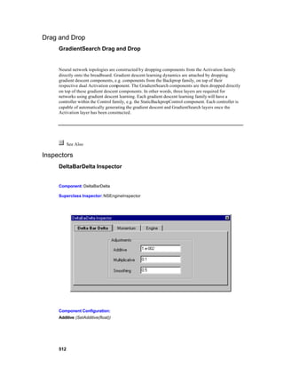

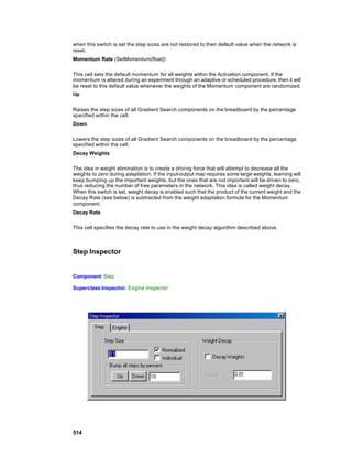
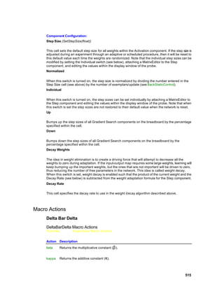

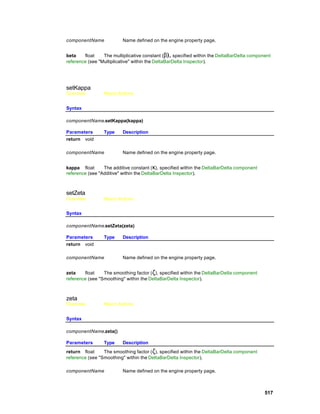
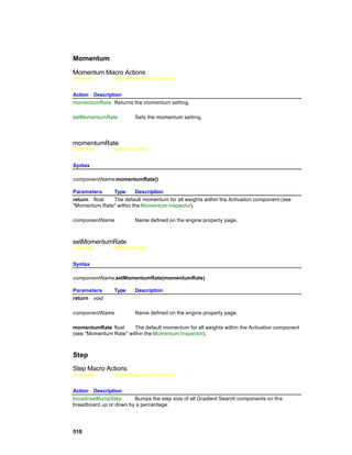


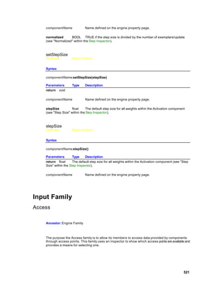

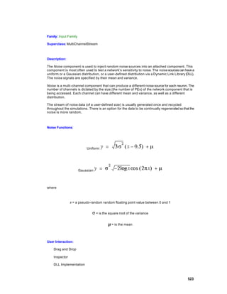


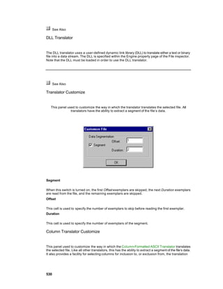
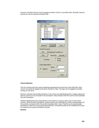


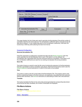


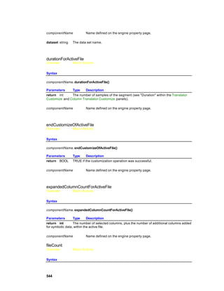

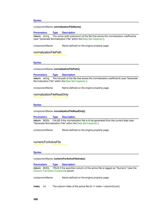
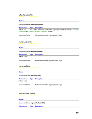

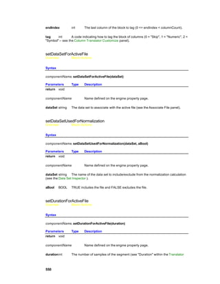
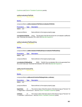
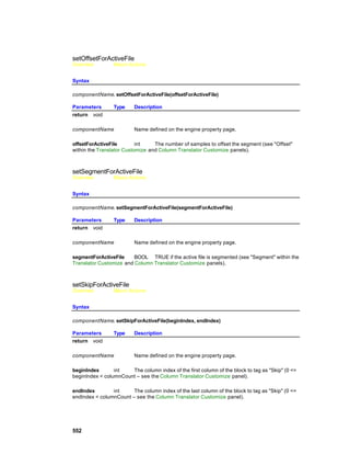

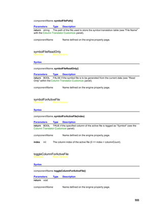
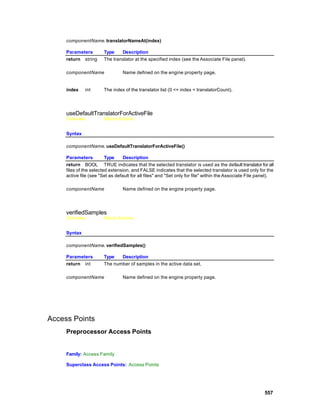

![Description:
The DLLInput component is used to inject data into the network from a DLL. This is similar to using
the DLL capability of the Function component, except that this data is not cyclical. One important
use for this feature is to retrieve input data from external hardware (such as an analog-to-digital
converter) by including the data acquisition code within the performInput function call.
The default implementa tion of this DLL simply fills the input buffer with zeros.
Code:
void performInput(
DLLData *instance, // Pointer to instance data (may be NULL)
NSFloat *data, // Pointer to the data
int rows, // Number of rows of data
int cols // Number of cols of data
)
{
int i,j;
for (i=0; i<rows; i++)
for (j=0; j<cols; j++)
data[i][j] = 0.0f; // You define your own input
source.
}
DLLPreprocessor & DLLPostprocessor DLL Implementation
Components: DLLPreprocessor, DLLPostprocessor
Protocol: PerformPrePost
Description:
The DLLPreprocessor and DLLPreprocessor components use the same protocol because their
functionality is very similar. The DLLPreprocessor is an input component that processes the input
data (using the Preprocessor access point) and injects it into the network. Conversely, the
DLLPostprocessor is a probe that processes data coming out of the network before sending it to
another probe (using the Postprocessor access point).
The default implementation of these DLLs simply copies the data coming in to the data going out.
Code:
560](https://image.slidesharecdn.com/neurosolutionshelp-090922003656-phpapp01/85/NeuroDimension-Neuro-Solutions-HELP-560-320.jpg)
![BOOL performPrePost(
DLLData *instance, // Pointer to instance data (may be NULL)
NSFloat *input // Pointer to the input data
NSFloat *output, // Pointer to the output data
int rows, // Number of rows of data
int cols // Number of cols of data
)
{
int i, length=rows*cols;
for (i=0; i<length; i++)
output[i] += input[i];
return TRUE; // Return whether to inject this sample or
// to call performPrePost with another sample
}
Drag and Drop
Access Drag and Drop
Components in the Access family will extract, inspect, or inject data reported by components via
access points. There are two basic forms of access points, static and temporal. An access point
may also be restricted to injecting of extracting data. The user however, is sheltered from these
complexities. When an Access component is dragged over top of another component, the mouse
cursor will change from a "not" sign to a stamp if the component will be accepted.
To find out what access points a component reports, reference its on-line help. Each component
that has access points will have a section describing them.
Input Drag and Drop
The members of the Input family are designed to inject data into the network via component
access points. These components can be dropped on any network component with an available
static input access point. The members of this family can also be stacked, allowing accumulated
input from multiple sources. Alternatively, stacking allows a probe to monitor the injected data.
Inspectors
Function Inspector
Component: Function
Superclass Inspector: Access inspector
561](https://image.slidesharecdn.com/neurosolutionshelp-090922003656-phpapp01/85/NeuroDimension-Neuro-Solutions-HELP-561-320.jpg)
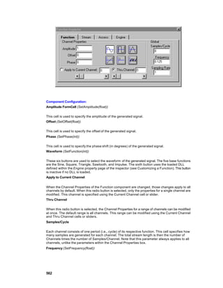
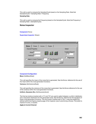
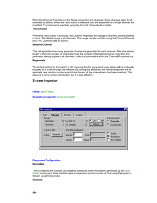
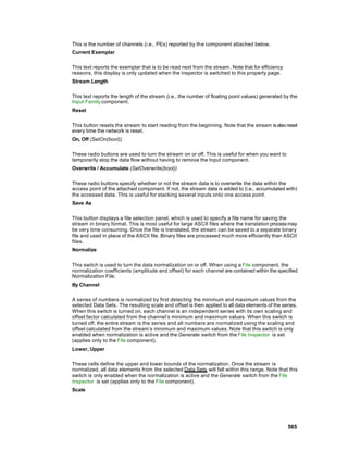


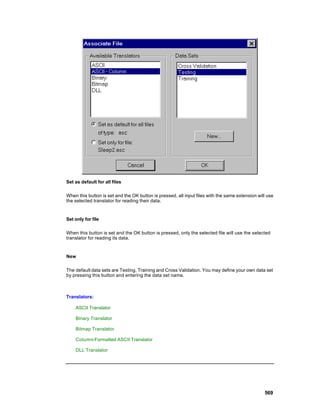

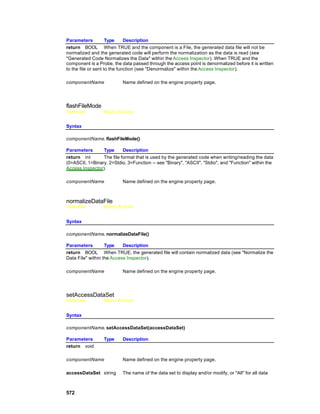
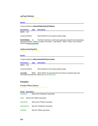
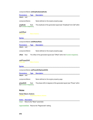

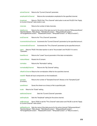

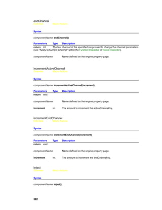
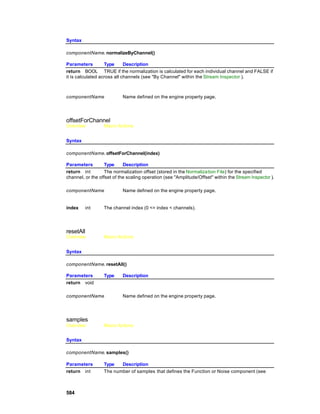
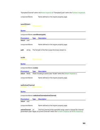
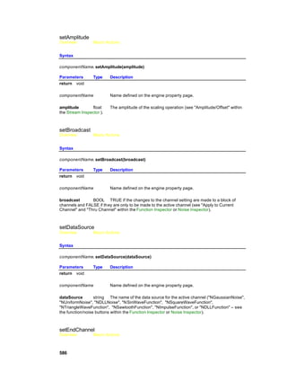
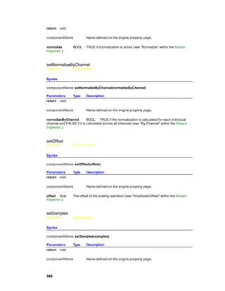


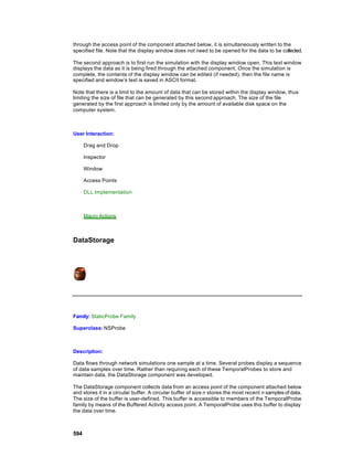


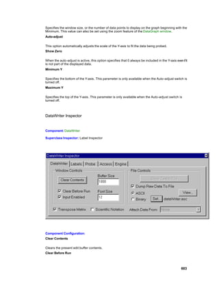
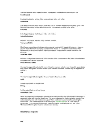


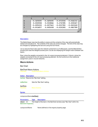


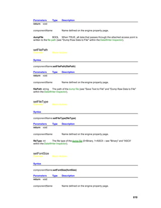


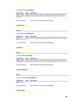
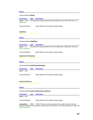


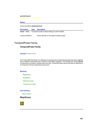


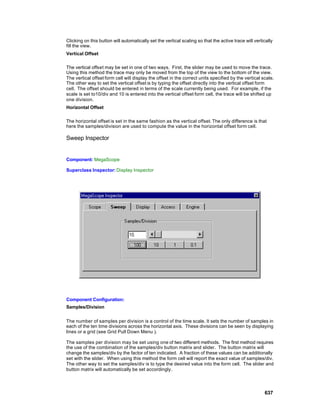
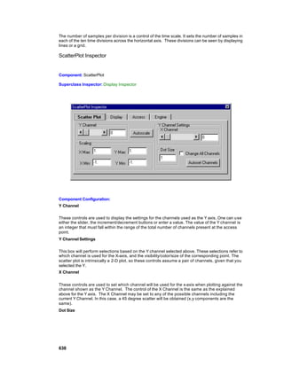
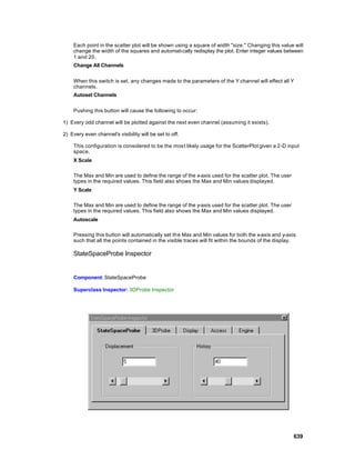
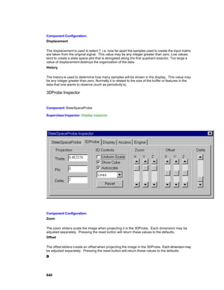


![setSweepMult Sets the sweep multiplier ([sweep rate] = [sweep multiplier] * 10 ^ [sweep scale]).
setSweepRate Sets the "Samples/Division" setting (sweep rate).
setSweepScale Sets the sweep scale ([sweep rate] = [sweep multiplier] * 10 ^ [sweep scale]).
setVerticalPos Sets the "Vertical Offset" scroller value.
setVerticalPosVolts Sets the "Vertical Offset" edit cell value.
sweepMult Returns the sweep multiplier (Sample/Division = [sweep multiplier] * 10 ^ [sweep
scale]).
sweepRate Returns the "Samples/Division" setting (sweep rate).
sweepScale Returns the sweep scale ([sweep rate] = [sweep multiplier] * 10 ^ [sweep scale]).
verticalPos Returns the "Vertical Offset" scroller value.
verticalPosVolts Returns the "Vertical Offset" edit cell value.
amplitude
Overview Macro Actions
Syntax
componentName.amplitude()
Parameters Type Description
return float The vertical scaling factor (see "Vertical Scale" of the Scope Inspector).
componentName Name defined on the engine property page.
autoscaleChannel
Overview Macro Actions
Syntax
componentName.autoscaleChannel()
Parameters Type Description
return void
componentName Name defined on the engine property page.
645](https://image.slidesharecdn.com/neurosolutionshelp-090922003656-phpapp01/85/NeuroDimension-Neuro-Solutions-HELP-645-320.jpg)
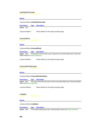

![return void
componentName Name defined on the engine property page.
sweepMult float The sweep multiplier ([sweep rate] = [sweep multiplier] * 10 ^ [sweep
scale] – see "Samples/Division" with the Sweep Inspector).
setSweepRate
Overview Macro Actions
Syntax
componentName.setSweepRate(sweepRate)
Parameters Type Description
return void
componentName Name defined on the engine property page.
sweepRate float The sweep rate ([sweep rate] = [sweep multiplier] * 10 ^ [sweep scale] –
see "Samples/Division" with the Sweep Inspector).
setSweepScale
Overview Macro Actions
Syntax
componentName.setSweepScale(sweepScale)
Parameters Type Description
return void
componentName Name defined on the engine property page.
sweepScale int The sweep scale ([sweep rate] = [sweep multiplier] * 10 ^ [sweep scale]
– see "Samples/Division" with the Sweep Inspector).
setVerticalPos
Overview Macro Actions
Syntax
componentName.setVerticalPos(verticalPos)
Parameters Type Description
return void
componentName Name defined on the engine property page.
649](https://image.slidesharecdn.com/neurosolutionshelp-090922003656-phpapp01/85/NeuroDimension-Neuro-Solutions-HELP-649-320.jpg)
![verticalPos float The position of the scroller used to adjust the vertical offset (see
"Vertical Offset" within the Scope Inspector).
setVerticalPosVolts
Overview Macro Actions
Syntax
componentName.setVerticalPosVolts(verticalPosVolts)
Parameters Type Description
return void
componentName Name defined on the engine property page.
verticalPosVolts float The value of the edit cell used to define the vertical offset (see "Vertical
Offset" within the Scope Inspector).
sweepMult
Overview Macro Actions
Syntax
componentName.sweepMult()
Parameters Type Description
return float The sweep multiplier ([sweep rate] = [sweep multiplier] * 10 ^ [sweep scale] – see
"Samples/Division" with the Sweep Inspector).
componentName Name defined on the engine property page.
sweepRate
Overview Macro Actions
Syntax
componentName.sweepRate()
Parameters Type Description
return float The sweep rate ([sweep rate] = [sweep multiplier] * 10 ^ [sweep scale] – see
"Samples/Division" with the Sweep Inspector).
componentName Name defined on the engine property page.
sweepScale
Overview Macro Actions
650](https://image.slidesharecdn.com/neurosolutionshelp-090922003656-phpapp01/85/NeuroDimension-Neuro-Solutions-HELP-650-320.jpg)
![Syntax
componentName.sweepScale()
Parameters Type Description
return int The sweep scale ([sweep rate] = [sweep multiplier] * 10 ^ [sweep scale] – see
"Samples/Division" with the Sweep Inspector).
componentName Name defined on the engine property page.
verticalPos
Overview Macro Actions
Syntax
componentName.verticalPos()
Parameters Type Description
return float The position of the scroller used to adjust the vertical offset (see "Vertical Offset"
within the Scope Inspector).
componentName Name defined on the engine property page.
verticalPosVolts
Overview Macro Actions
Syntax
componentName.verticalPosVolts()
Parameters Type Description
return float The value of the edit cell used to define the vertical offset (see "Vertical Offset"
within the Scope Inspector).
componentName Name defined on the engine property page.
Scatter Plot
ScatterPlot Macro Actions
Overview Superclass Macro Actions
Action Description
autoSetUpChannels Automatically sets every odd channel to be plotted against the next
even channel (assuming it exists), and every even channel’s visibility will be set to off (see "Autoset
Channels" within the ScatterPlot Inspector).
decrementXChannel Decreases the "X Channel" setting by one (see "X Channel" within the
ScatterPlot Inspector).
651](https://image.slidesharecdn.com/neurosolutionshelp-090922003656-phpapp01/85/NeuroDimension-Neuro-Solutions-HELP-651-320.jpg)

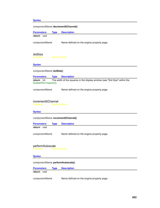


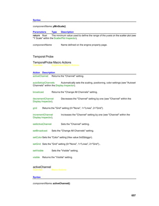
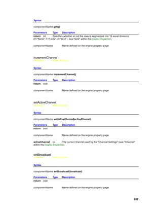

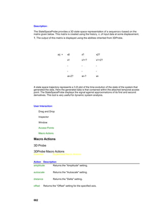


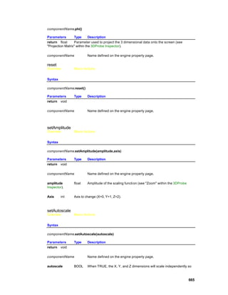

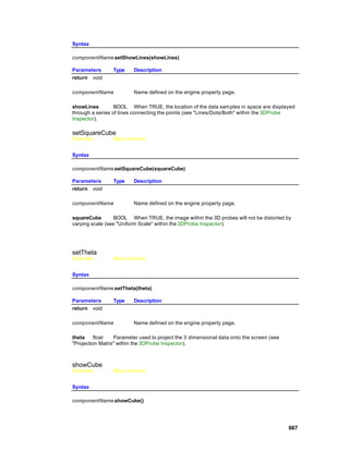


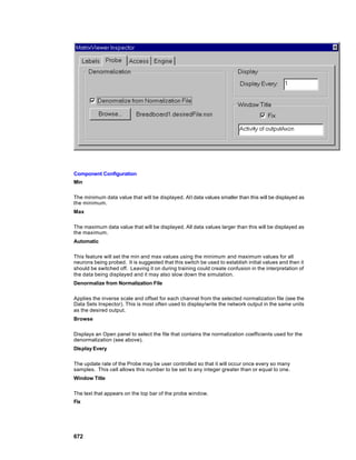


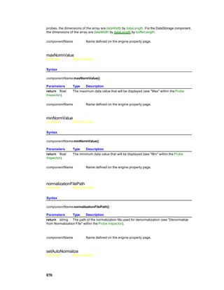
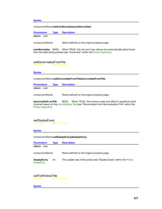


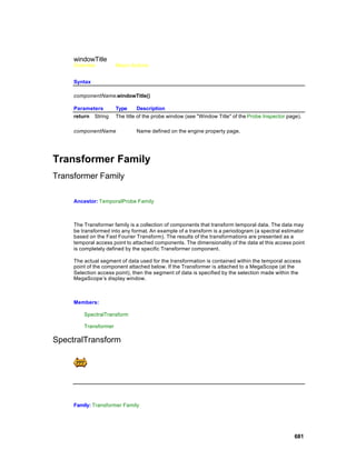


![DLLData *instance, // Pointer to instance data
NSFloat *data, // Pointer to the buffered data
int length, // Length of the buffer to be transformed
int channel // Current channel number
)
{
int i;
for (i=0; i<length; i++)
data[i] = 0.0f; // transform the data here
// Return whether or not to display this channel
return TRUE;
}
Inspectors
SpectralTransform Inspector
Component: SpectralTransform
Superclass Inspector: Display Inspector
Component Configuration:
FFT Size
The FFT Size may be set to any power of 2 greater than 2 and less than or equal to 4096. If a
value that is not a power of 2 is entered into the form cell, the next largest power of 2 will be used.
If the amount of data specified by the window size is smaller than the FFT size, zero padding will
be used to get the appropriate number of points (power of 2).
Overlap
684](https://image.slidesharecdn.com/neurosolutionshelp-090922003656-phpapp01/85/NeuroDimension-Neuro-Solutions-HELP-684-320.jpg)

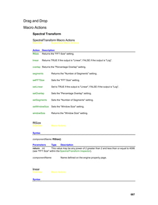


![See Also
DLL Implementation
ExpScheduler DLL Implementation
Component: ExpScheduler
Protocol: PerformScheduler
Description:
This function is called after each epoch that has scheduling active (specified by the user within the
Scheduler inspector). It simply multiplies each PE within data by beta and copies the result back
into data. Note that the component itself handles the clipping if the data exceeds the boundaries
specified by the user.
Code:
BOOL performScheduler(
DLLData *instance, // Pointer to instance data (may be NULL)
NSFloat *data, // Pointer to the data to be scheduled
int length, // Number of elements in scheduled data vector
NSFloat beta // Scheduler parameter (specified by user)
)
{
int i;
for (i=0; i<length; i++)
data[i] = beta*data[i];
}
LinearScheduler DLL Implementation
693](https://image.slidesharecdn.com/neurosolutionshelp-090922003656-phpapp01/85/NeuroDimension-Neuro-Solutions-HELP-693-320.jpg)
![Component: LinearScheduler
Protocol: PerformScheduler
Description:
This function is called after each epoch that has scheduling active (specified by the user w ithin the
Scheduler inspector). It simply increments each PE within data by beta. Note that the component
itself handles the clipping if the data exceeds the boundaries specified by the user.
Code:
BOOL performScheduler(
DLLData *instance, // Pointer to instance data (may be NULL)
NSFloat *data, // Pointer to the data to be scheduled
int length, // Number of elements in scheduled data vector
NSFloat beta // Scheduler parameter (specified by user)
)
{
int i;
for (i=0; i<length; i++)
data[i] += beta;
}
LogScheduler DLL Implementation
Component: LogScheduler
Protocol: PerformScheduler
Description:
This function is called after each epoch that has scheduling active (specifi ed by the user within the
Scheduler inspector). It simply decrements each PE within data by beta over data. Note that the
component itself handles the clipping if the data exceeds the boundaries specified by the user.
Code:
BOOL performScheduler(
DLLData *instance, // Pointer to instance data (may be NULL)
NSFloat *data, // Pointer to the data to be scheduled
694](https://image.slidesharecdn.com/neurosolutionshelp-090922003656-phpapp01/85/NeuroDimension-Neuro-Solutions-HELP-694-320.jpg)
![int length, // Number of elements in scheduled data vector
NSFloat beta // Scheduler parameter (specified by user)
)
{
int i;
for (i=0; i<length; i++)
data[i] -= beta / data[i];
}
Inspectors
Schedule Inspector
Family: Schedule Family
Superclass Inspector: Access inspector
Component Configuration:
Start at Epoch (SetStartAt(int))
This cell is used to specify when the scheduling is to begin based on the epoch count.
Until Epoch (SetUntil(int))
This cell is used to specify when the scheduling is to end based on the epoch count.
Beta (SetBeta(float))
This cell is used to specify β . This parameter determines the rate of change of the scheduled
variable. The schedule equation of the component reference defines how this parameter is used to
compute the variable’s current value based on its previous value.
Minimum (SetMin(float))
695](https://image.slidesharecdn.com/neurosolutionshelp-090922003656-phpapp01/85/NeuroDimension-Neuro-Solutions-HELP-695-320.jpg)


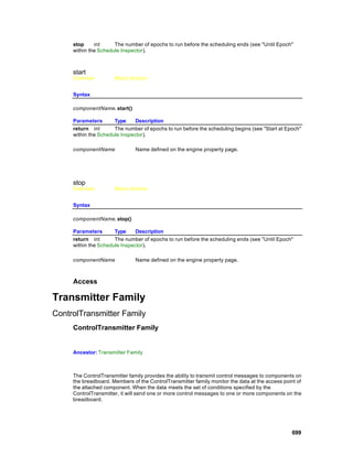
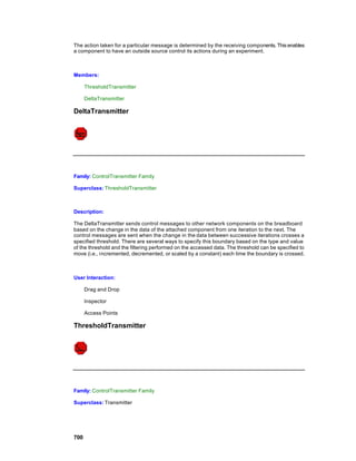

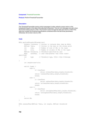
![register int i;
for (i=0; i<length; i++)
if (data[i] < threshold)
return YES;
return NO;
}
BOOL allLessThan(NSFloat *data, int length, NSFloat threshold)
{
register int i;
for (i=0; i<length; i++)
if (data[i] > threshold)
return NO;
return YES;
}
BOOL averageLessThan(NSFloat *data, int length, NSFloat threshold)
{
register int i;
register NSFloat average = (NSFloat)0.0;
for (i=0; i<length; i++)
average += data[i];
return (average /= length) < threshold;
}
Inspectors
ThresholdTransmitter Inspector
Component: ThresholdTransmitter
Superclass Inspector: Transmitter Inspector
703](https://image.slidesharecdn.com/neurosolutionshelp-090922003656-phpapp01/85/NeuroDimension-Neuro-Solutions-HELP-703-320.jpg)

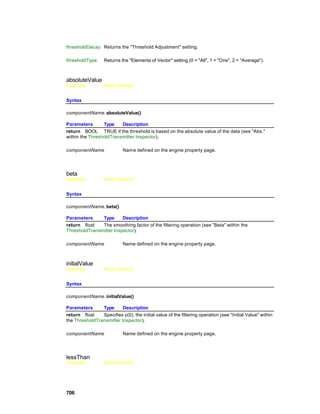
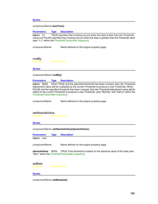

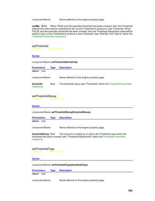


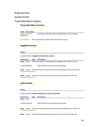

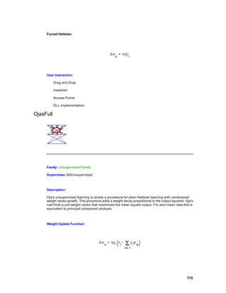


![DLL Implementation
Competitive DLL Implementation
Components: StandardFull, ConscienceFull
Protocol: PerformCompetitive
Description:
The StandardFull and ConscienceFull components implement competitive learning. The
ConscienceFull component differs from the StandardFull in that the former adds a bias (i.e., a
"conscience") to the competition with the goal of equilibrating the winnings. Note that this second
level of competition is performed by the ConscienceFull component to determine the winner, and is
not part of code below. This code updates the weights that are connected to the winning output PE.
Code:
void performCompetitive(
DLLData *instance, // Pointer to instance data (may be NULL)
NSFloat *input, // Pointer to the input layer of PEs
int inRows, // Number of rows of PEs in the input layer
int inCols, // Number of columns of PEs in the input layer
NSFloat *output, // Pointer to the output layer
int outRows, // Number of rows of PEs in the output layer
int outCols // Number of columns of PEs in the output
layer
NSFloat *weights // Pointer to the fully-connected weight
matrix
NSFloat step // Learning rate
int winner // Index of winning PE
)
{
int i,
inCount=inRows*inCols,
outCount=outRows*outCols;
for (i=0; i<inCount; i++)
W(winner,i) += step*(input[i] - W(winner,i));
}
720](https://image.slidesharecdn.com/neurosolutionshelp-090922003656-phpapp01/85/NeuroDimension-Neuro-Solutions-HELP-720-320.jpg)
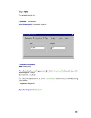
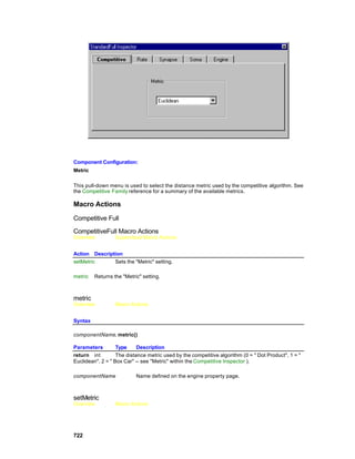
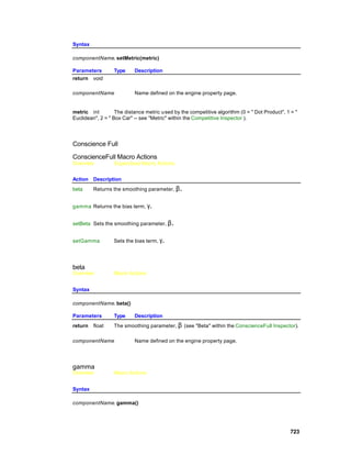


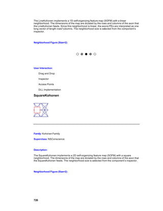


![void performKohonen(
DLLData *instance, // Pointer to instance data (may be NULL)
NSFloat *input, // Pointer to the input layer of PEs
int inRows, // Number of rows of PEs in the input layer
int inCols, // Number of columns of PEs in the input layer
NSFloat *output, // Pointer to the output layer
int outRows, // Number of rows of PEs in the output layer
int outCols // Number of columns of PEs in the output
layer
NSFloat *weights // Pointer to the fully-connected weight
matrix
NSFloat step // Learning rate
int winningRow, // Index of winning row
int winningCol, // Index of winning column
int size // Size of the neighborhood
)
{
int i,j,k,
inCount = inRows*inCols,
startRow = winningRow - size,
stopRow = winningRow + size,
startCol = winningCol - size,
stopCol = winningCol + size;
if (startRow < 0)
startRow = 0;
if (stopRow >= outRows)
stopRow = outRows-1;
if (startCol < 0)
startCol = 0;
if (stopCol >= outCols)
stopCol = outCols-1;
for (i=startRow; i<stopRow; i++)
for (j=startCol; j<stopCol; j++)
if (abs(i-winningRow) + abs(j-winningCol) <= size)
for (k=0; k<inCount; k++)
W(j+i*outCols,k) += step*(input[k] -
W(j+i*outCols,k));
}
LineKohonen DLL Implementation
729](https://image.slidesharecdn.com/neurosolutionshelp-090922003656-phpapp01/85/NeuroDimension-Neuro-Solutions-HELP-729-320.jpg)
![Component: LineKohonen
Protocol: PerformKohonen
Description:
The LineKohonen component implements a 1D self-organizing feature map (SOFM) with a linear
neighborhood. The dimensions of the map are dictated by the vector length (outRows*outCols) of
the axon that the LineKohonen feeds. The neighborhood size is defined by the user within the
component’s inspector.
Code:
void performKohonen(
DLLData *instance, // Pointer to instance data (may be NULL)
NSFloat *input, // Pointer to the input layer of PEs
int inRows, // Number of rows of PEs in the input layer
int inCols, // Number of columns of PEs in the input layer
NSFloat *output, // Pointer to the output layer
int outRows, // Number of rows of PEs in the output layer
int outCols // Number of columns of PEs in the output
layer
NSFloat *weights // Pointer to the fully-connected weight
matrix
NSFloat step // Learning rate
int winningRow, // Index of winning row
int winningCol, // Index of winning column
int size // Size of the neighborhood
)
{
int i,j,
inCount = inRows*inCols,
outCount = outRows * outCols,
winner = winningCol + winningRow*outCols,
start = winner - size,
stop = winner + size;
if (start < 0)
start = 0;
if (stop >= outCount)
stop = outCount-1;
for (i=start; i<=stop; i++)
for (j=0; j<inCount; j++)
W(i,j) += step*(input[j] - W(i,j));
}
SquareKohonen DLL Implementation
730](https://image.slidesharecdn.com/neurosolutionshelp-090922003656-phpapp01/85/NeuroDimension-Neuro-Solutions-HELP-730-320.jpg)
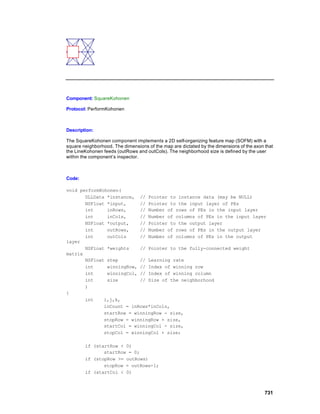
![startCol = 0;
if (stopCol >= outCols)
stopCol = outCols-1;
for (i=startRow; i<=stopRow; i++)
for (j=startCol; j<=stopCol; j++)
for (k=0; k<inCount; k++)
W(j+i*outCols,k) += step*(input[k] -
W(j+i*outCols,k));
}
Inspectors
Kohonen Inspector
Superclass Inspector: Conscience Inspector
Component Configuration:
Neighborhood (SetNeighborhood(int))
This cell specifies the size of the spatial neighborhood used by the Kohonen algorithm. See the
Neighborhood Figure section of the component reference for its use of this parameter.
Beta (SetBeta(float))
See Conscience Inspector
Gamma (SetGamma(float))
See Conscience Inspector
Component Plane (setComponentPlane(int))
Used to select the plane displayed by the probe attached to the Component Plane access point.
732](https://image.slidesharecdn.com/neurosolutionshelp-090922003656-phpapp01/85/NeuroDimension-Neuro-Solutions-HELP-732-320.jpg)

![Component: HebbianFull
Protocol: PerformUnsupervised
Description:
The HebbianFull component implements Plain Hebbian and Forced Hebbian learning. Each weight
of the fully-connected matrix is adjusted by adding the product of the activity at the output PE, the
activity at the input PE, and the step size.
Code:
void performUnsupervised(
DLLData *instance, // Pointer to instance data (may be NULL)
NSFloat *input, // Pointer to the input layer of PEs
int inRows, // Number of rows of PEs in the input layer
int inCols, // Number of columns of PEs in the input layer
NSFloat *output, // Pointer to the output layer
int outRows, // Number of rows of PEs in the output layer
int outCols // Number of columns of PEs in the output layer
NSFloat *weights // Pointer to the fully-connected weight matrix
NSFloat step // Learning rate
)
{
int i, j,
inCount=inRows*inCols,
outCount=outRows*outCols;
for (j=0; j<inCount; j++)
for (i=0; i<outCount; i++)
W(i,j) += step*input[j]*output[i];
}
OjasFull DLL Implementation
Component: OjasFull
Protocol: PerformUnsupervised
735](https://image.slidesharecdn.com/neurosolutionshelp-090922003656-phpapp01/85/NeuroDimension-Neuro-Solutions-HELP-735-320.jpg)
![Description:
OjasFull implements plain Hebbian learning with constrained weight vector growth. This procedure
adds a weight decay proportional to the output squared. The implementation is similar to that of the
DLL Implementation component, except that each input PE term used to compute the weight
change is reduced by the sum of products of the output PEs and the weights connected to the
given input.
Code:
void performUnsupervised(
DLLData *instance, // Pointer to instance data (may be NULL)
NSFloat *input, // Pointer to the input layer of PEs
int inRows, // Number of rows of PEs in the input layer
int inCols, // Number of columns of PEs in the input layer
NSFloat *output, // Pointer to the output layer
int outRows, // Number of rows of PEs in the output layer
int outCols // Number of columns of PEs in the output layer
NSFloat *weights // Pointer to the fully-connected weight matrix
NSFloat step // Learning rate
)
{
int i, j,
inCount=inRows*inCols,
outCount=outRows*outCols;
NSFloat partialSum;
for (j=0; j<inCount; j++) {
partialSum = (NSFloat)0;
for (i=0; i<outCount; i++)
partialSum += output[i] * W(i,j);
for (i=0; i<outCount; i++)
W(i,j) += step*output[i]*(input[j] - partialSum);
}
}
SangersFull DLL Implementation
Component: SangersFull
Protocol: PerformUnsupervised
736](https://image.slidesharecdn.com/neurosolutionshelp-090922003656-phpapp01/85/NeuroDimension-Neuro-Solutions-HELP-736-320.jpg)
![Description:
SangersFull implements principal component analysis. It does this with a plain Hebbian weight
update rule while constraining the growth of the weight vector, similar to the DLL Implementation
component. The difference is that the range of the summation has changed, resulting in an
ordering of the principal components.
Code:
void performUnsupervised(
DLLData *instance, // Pointer to instance data (may be NULL)
NSFloat *input, // Pointer to the input layer of PEs
int inRows, // Number of rows of PEs in the input layer
int inCols, // Number of columns of PEs in the input layer
NSFloat *output, // Pointer to the output layer
int outRows, // Number of rows of PEs in the output layer
int outCols // Number of columns of PEs in the output layer
NSFloat *weights // Pointer to the fully-connected weight matrix
NSFloat step // Learning rate
)
int i, j,
inCount=inRows*inCols,
outCount=outRows*outCols;
NSFloat partialSum;
for (j=0; j<inCount; j++) {
partialSum = (NSFloat)0;
for (i=0; i<outCount; i++) {
partialSum += output[i] * W(i,j);
W(i,j) += step*output[i]*(input[j] - partialSum);
}
}
}
Drag and Drop
Unsupervised Drag and Drop
All components in the Unsupervised family must be dropped directly on a component from the
Synapse family. The unsupervised component will then be positioned in the upper left corner of
the synapse.
See Also
737](https://image.slidesharecdn.com/neurosolutionshelp-090922003656-phpapp01/85/NeuroDimension-Neuro-Solutions-HELP-737-320.jpg)


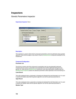


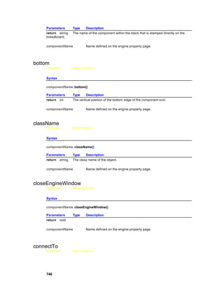
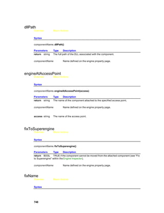
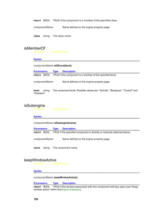

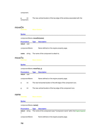
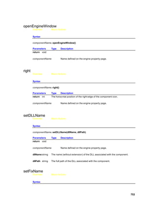


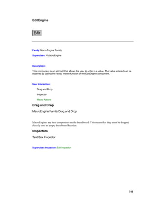

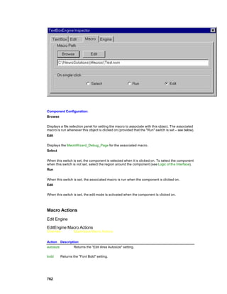

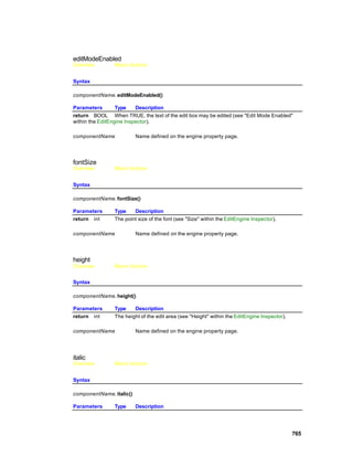


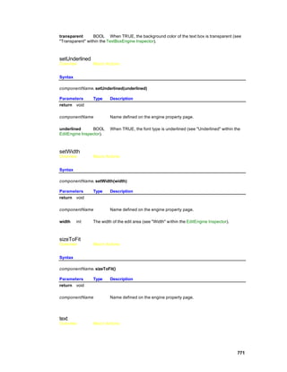

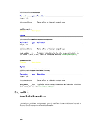
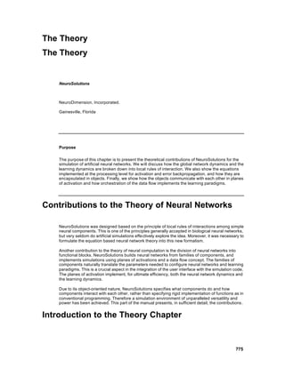
![The simulation of artificial neural networks (ANNs) is an increasingly important research area. This
is due to the demanding computer bandwidth of ANN implementations coupled with the need to
experimentally test topologies and parameters. This compensates, in part, a lack of thorough
theoretical characterization of ANNs. The need to address real world applications implies a
requirement for simulating very large networks. The simulation environments must not only be fast
and efficient, but also user friendly and upgradeable, enabling thorough experimental validation.
With the computational bandwidth requirements, brute force implementation can give unrealistic
computation times, even using supercomputers. Careful planning and fine-tuning of the code has
been a necessity for ANN implementations in digital computers.
At first we looked at the problem from a mere engineering perspective, i.e. to find what
computational models were most natural for an efficient implementation of ANN topologies. Our
conclusion is that an object-oriented programming paradigm conforms to topologies made up of
aggregates of similar elements instantiated as many times as necessary. Along the way we found
out that object-oriented concepts provide an alternate and equivalent description of ANN paradigms
much more appropriate for simulating ANN topologies.
An ANN model is described by a set of dynamic equations. Being adaptive systems, ANNs require
a second set of dynamic equations for learning. Although these equations translate the potential
and concepts of the theoretical model very well, they suffer from a key shortcoming. ANNs are
implemented in digital computers or other hardware through topologies. A given ANN model may
produce several topologies. For each topology the equation-based description applies, but at the
expense of brute force calculations and exaggerated storage requirements.
Consider the multilayer perceptron (MLP) [Lippman, 1987] and Hopfield network [Hopfield, 1982].
As topologies, they differ substantially (one is feedforward while the other is recurrent), but they are
two implementations for the additive model (in the sense of Grossberg [Grossberg, 1983]).
Therefore, if a useful implementation for the additive model is developed in a digital computer, it
can implement an MLP and a Hopfield network indiscriminately (or any other recurrent topology).
The implementations, however, will be very inefficient since, in the MLP, the feedback connections
are set at zero, while the connections in recurrent networks are normally sparse. The same
argument applies to learning dynamics, i.e. gradient descent learning for these two networks.
Furthermore, when implementing the learning rules one ends up with two distinctly different
learning procedures, since the MLP is static and the Hopfield network is recurrent.
This example may be generalized to show that learning equations are specific to topologies and
becomes obvious when the transpose network is used to propagate errors and compute gradients
(one of the leading contributions from neural network theory to gradient descent learning). It may
seem that for the sake of efficiency we are restricted to customized simulation environments, with
code specifically written for each network topology and learning paradigm. But we think otherwise,
and NeuroSolutions is a "living proof" of such beliefs.
The major goal of this document is to present a simulation environment for neural networks which
consists of a mixture of feedforward and recurrent sub-networks, trained with static
backpropagation, fixed point learning, or backpropagation through time (BPTT). In our opinion, the
equation based modeling, so widespread in ANNs, has an alternate and equivalent formulation,
which we call object-oriented modeling, and which is far more natural for computer, based
simulations of ANNs. Object-oriented modeling is achieved by the execution of an ordered
sequence of formal procedures. At present, we utilize digital computers as the engines for object-
oriented modeling. This equivalence is predicated on the well known but often overlooked fact that
ANN interactions are BOTH local to space (finite elemental topologies) and to time neighborhoods
(finite data operators), which we refer to as being local in time and in space. The equation-based
modeling does not explore this natural fact, but object-oriented modeling does. Neural network
behavior can be easily encoded into local dynamic rules of interaction. These elementary rules are
simply replicated across the network. In this sense the ANN with its learning rules operates as a
cellular automaton or a lattice in time and space.
A lattice in mathematics is a partially ordered set (with some constraints [Birkhoff, 1948]). Here we
will be using the term to represent an ensemble of ordered computations that can be mapped to
sites in a graph. Some of these sites may als o require ordered computations in time (such as linear
filtering operations), so the overall simulation structure is a coupled lattice.
776](https://image.slidesharecdn.com/neurosolutionshelp-090922003656-phpapp01/85/NeuroDimension-Neuro-Solutions-HELP-776-320.jpg)
![Equation-based Modeling
Every neural network researcher has been faced with the problem of translating equations that
describe ANN dynamics to computer programs that implement the network topology. The synthetic
power and formalism embedded in a mathematical expression is hard to beat, and has been
extensively used for characterizing the global dynamics of neural models. Until the advent of
computers, mathematics was the most utilized formal descriptive system. We should remember,
however, that computer languages are also formal systems and possess the same properties.
A computer algorithm describes a relationship as precisely as a mathematical formula. The
problem is one of choosing the representation that best suits our needs. We do not dispute that at
the modeling level, equations are the best way to translate global dynamic properties of the
interactions. But does this extrapolate to implementations, i.e. to neural network simulations? Let
us examine this point in more detail using the additive model as an example [Amari, 1972,
Grossberg, 1973]. In modeling, dynamics are described by coupled sets of first order nonlinear
differential equations of the form,
where is the systems state vector, is a dynamic map, is an external input,
represents internal system parameters and is a desired trajectory for the
system’s state. A neural model is adopted by selecting a distributed set of dynamic mapping
functions for the system’s state vector. For the additive model, we have,
where is the time constant of the ith processing element and is its input-output
transfer function.
In a block diagram this can be illustrated as the block additive model in the figure below (all
quantities are vectors). Although this model is very general, notice that the activation at node i only
depends explicitly on the present input. This feature is undesirable for a large class of problems
such as the classification of time varying signals (speech, control, and prediction). One way of
modifying the additive model is to substitute the multiplications by convolutions in time
777](https://image.slidesharecdn.com/neurosolutionshelp-090922003656-phpapp01/85/NeuroDimension-Neuro-Solutions-HELP-777-320.jpg)
![This model has been called the convolution model [deVries and Principe, 1992], and allows the
ANN activations to depend explicitly upon the past of the input signal and/or model states. The
convolution is a linear operation, so conceptually one can picture the neural activations being
stored into a general linear filter, which unfortunately has a growing number of coefficients.
Gamma neural model as a prewired additive model
The convolution model can be approximated by fixed order structures [deVries and Principe, 1992].
They showed that the gamma neural model,
for sufficiently large K can approximate the convolution model as close as necessary. These
equations can be easily extended to discrete time [deVries and Principe, 1992]. Special cases of
this recursive memory structure are the tapped delay line for µ =1 (utilized in the time domain
neural network- TDNN, [Lang et al, 1990]), and context unit for K=1 [Jordan, 1986].
A neural network is an implementation of a neural model. Normally a topology is assigned by
choosing specific forms of the weight matrix (i.e. fully populated weight matrices give rise to
recurrent nets, and when all the weights with i?j are zero, feedforward nets).
The learning dynamics in the N -dimensional dynamic system of the equation above also involves
translating equations to network topologies, although some papers have been written with the word
778](https://image.slidesharecdn.com/neurosolutionshelp-090922003656-phpapp01/85/NeuroDimension-Neuro-Solutions-HELP-778-320.jpg)
!["general" in the title [Thrun and Smieja, 1991]. When present, the vector is used to represent
the target values for the desired output. In this framework, learning consists of adjusting the weight
values such that the desired output is obtained. Notice that this output can be a function of time, or
a constant value.
When the goal is to match a d esired response, a metric must be established in the error, i.e. the
difference between the desired and actual output. This problem has been extensively studied in
adaptive signal processing [Haykin, 1991] and optimal control [Bryson and Ho, 1975]. The standard
metric chosen is the L2 norm (mean square error), and the method normally used to minimize this
error is gradient descent. In gradient descent learning, network coefficients are updated according
to the formula,
where E is an error functional, and η is the learning rate.
In order to proceed we must know more about the problem under different learning methods (static
backpropagation [Rumelhart et al, 1986], fixed point learning [Pineda, Almeida, 1987],
backpropagation through time [Werbos, 1990], and real time recurrent learning [William and Zipser,
1989). For one thing, the error is a function of the network output, which is coupled directly to the
network topology. The desired signal can be a constant (fixed point) or time varying (a trajectory).
This implies two possibilities: either the network is feedforward and the desired signal and network
inputs are static, in which case the gradient computations are independent of time; or the network
is recurrent and/or the desired signal is time dependent in which case the gradient computation
becomes time dependent. Normally in the ANN literature, these cases are divided into the learning
methods mentioned above. A detailed discussion of the methods is outside the scope of this work.
What we want to stress is the following facts: First, the network topology affects the equations that
compute the gradients. Second, in all these methods, the gradient can be computed with local
information, both spatially and temporally.
Let us summarize what we have reviewed. In the figure below (left half) we show diagrammatically
how the analysis progressed, from the model to the topology (network), to the learning system. The
network is a special implementation of the model. Since learning uses the network it will also
become a special case for each topology. For this reason we believe that if a new topology
encapsulates a unique feature of the neural model, it will always require a special set of equations
to describe it.
779](https://image.slidesharecdn.com/neurosolutionshelp-090922003656-phpapp01/85/NeuroDimension-Neuro-Solutions-HELP-779-320.jpg)
![Equation vs. object-oriented based methodology
Also in the figure above (right half) we present an alternate route that we call object-oriented
modeling. Due to the fact that interactions are local, let us first capture the simplest dynamic
interactions at the processing element level, which we called the elemental neural dynamics. From
the elemental neural dynamics we can glue together elemental topologies, or full-blown neural
networks. The elemental dynamics will define local rules of interaction relating the processing of
neural activity. Additional rules of interaction will have to be defined which allow these elemental
topologies to exist in a data flow machine.
These rules of interaction will be solving the equations that we have seen for ANN models, but in
object-oriented modeling we do not need to write them explicitly. This is the main difference
between the two approaches. Our point is that once the quantitative and theoretical aspects of
neural modeling are understood, we do not need to go back to the equations every time we
implement an ANN simulation. We can construct topologies and, for efficiency, fully utilize the local
structure of the networks. The number of elementary dynamics required by this method to simulate
all topologies for a neural model turned out to be small, and different neural models will decompose
into the same elementary dynamics [Lefebvre and Principe, 1993]. A final comment relates to the
coding of this scheme in a computer language. Notice that we propose building networks by placing
together similar elements. This is the software equivalent of building electronic circuits. Therefore,
an object oriented paradigm where a hierarchy of classes recursively encapsulate standard rules of
interaction makes perfect sense. Network topologies will be constructed by simply interconnecting
a small number of instantiated classes. The user can simply arrange neural elements on
breadboards.
Object-oriented Modeling of Neural Networks
Object-oriented Modeling of Neural Networks
The first step in object-oriented modeling of ANNs is to characterize an abstract set of elements
which constitute arbitrary neural functions and which standardize rules for local interaction.
Therefore we must analyze what is the most general element that one may wish to construct. The
fundamental element in artificial neural networks is the processing element (PE) based on the
780](https://image.slidesharecdn.com/neurosolutionshelp-090922003656-phpapp01/85/NeuroDimension-Neuro-Solutions-HELP-780-320.jpg)
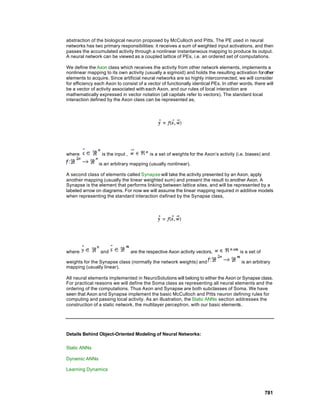


![As an illustration, lets implement the focused gamma neural network using this coupled l attice. A
focused gamma network is a topology that has a gamma memory structure in the input layer
(storing traces of the input signal) followed by an MLP [Principe et al, 1992]. If we examine the
gamma neural model equation, we see that the gamma neural m odel is simply an additive model
with gamma memory structures inserted for arbitrary states. Let us take a closer look at a discrete
version of the gamma memory structure,
Within this equation we see two delayed synaptic maps, one between adjacent memory states (
is a function of activation at the previous time) and one recurrently feeding each memory
state onto itself ( is a function of at the previous time). However both of these maps follow
the same elementary form given by,
where is a vector of coefficients. In other words, this Synapse will apply a bijective (one-to-
one and onto) linear map between Axon sites in the lattice. We can immediately construct the
lattice for a focused gamma network as in the figure below. In this figure, (t) is the input, (t)
represents the hidden layer and (t) is the network output.
Notice that the recursive nature of the gamma memory could in principle require an extension of
the instantaneous mapping properties of the Axon class. In the proposed distribution of dynamics
the Axon has no knowledge of temporal information, the Soma is responsible for handling time.
785](https://image.slidesharecdn.com/neurosolutionshelp-090922003656-phpapp01/85/NeuroDimension-Neuro-Solutions-HELP-785-320.jpg)
![Focused gamma network on coupled lattice
This simple trick allows each elementary map to be applied over spatial and/or temporal
displacements without modification; i.e. all elements are implemented as if they were instantaneous
mappers. An Axon will fire when all contributions from the present and delayed inputs are received.
This implies that all sites in the delayed spatial planes will fire immediately at each increment in
time.
We just presented two examples of topologies belonging to the additive model. In so doing we have
defined ALL the operators that are needed to build ANY topology conforming to the additive model
dynamics. This can be demonstrated in general for most neural models and mathematically proven
using the formalism of graph theory [Lefebvre, 1992], but probably a more insightful discussion
would be to relate this to other areas where similar procedures are used.
For instance in electronics, with capacitors, resistors, inductors and amplifiers, one can build any
linear filter by topologically arranging the elements. The same has been accomplished through
object-oriented modeling for artificial neural networks. We now have a library of elements that can
construct any ANN topology belonging to the additive model. Our examples have not explicitly
addressed globally recurrent networks, so as a final example lets consider the most general (linear
for simplicity) feedback model. The multivariate state variable model is probably the most widely
used description for recurrent systems,
where is the system’s state vector, is its input and is the output.
Notice that because of linearity, the only mapping used by this model is that of our fully connected
Synapse. If we create as instances of the fully connected
Synapse class, then the figure below will implement this state variable description. The state
variable description given above can be considered a specific topology belonging to the additive
model, where (this is the reason the Axon is not utilized).
We have accomplished an alternate description of ANNs as aggregates of McCulloch and Pitts
processing elements living in an ordered space of computations (the coupled lattice). This
description is equivalent to the equation-based description and is much more appropriate for
computer implementations. Notice that we can mix static and recurrent elements in a network
without the hassle of simulating global dynamic equations.
786](https://image.slidesharecdn.com/neurosolutionshelp-090922003656-phpapp01/85/NeuroDimension-Neuro-Solutions-HELP-786-320.jpg)

![For the Synapse class the transpose element is called the BackSynapse and its mapping is shown
in the figure below. You should compare these figures to the ones for the Axon mapping and the
Synapse mapping to see the transpose relationship.
BackSynapse map
The error is fed into the transpose system, and the propagating activities correspond to the error
gradient with respect to activities of the forward network which will be denoted by,
Proof that activities in the transpose system correspond to follow directly from application of
the chain rule for ordered partial derivatives backwards through all nodes of the forward system
[Werbos, 1990] or from system theoretic concepts [Almeida, 1987]. The chain rule is given by,
where i indexes space and t indexes time. Notice that the gradient at node i can be computed by
adding a direct contribution from the gradient at each internal node with the sum of indirect
contributions flowing to that node. Therefore, one can always compute the gradient at each node in
the lattice by information available in the neighboring nodes.
Gradient descent learning will require two tasks for each of our elementary dynamics: each must
add their effect to the error gradient being propagated, which we call its sensitivity function (this can
be described by the transpose system), and each must use that gradient to determine the effect its
internal coefficient had on the error, which we call the gradient function (this is what is used for
weight update). Therefore deriving learning rules for the elementary dynamic maps requires two
applications of the chain rule, one from the map’s output to its input (sensitivity function) and one
from its output to its coefficients (gradient function). For the BackAxon we get,
788](https://image.slidesharecdn.com/neurosolutionshelp-090922003656-phpapp01/85/NeuroDimension-Neuro-Solutions-HELP-788-320.jpg)
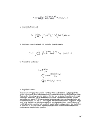
![There are several important benefits to this approach that we have tried to illustrate through these
examples. First, learning was derived directly from the elementary maps (of the Axon and Synapse
classes). Therefore, once you have arranged elements on the lattice, the learning dynamics can be
implemented by simply reversing the direction of data flow and replacing each elementary dynamic
with its learning equivalent.
Backpropagation network on coupled lattice
The figure above illustrates the transpose network for the focused gamma network figure. Notice
that time runs backwards in this network. This process of constructing the learning network can be
automated by the simulation environment, thus the user simply constructs the feedforward network
without ever having to address learning.
When modeling is based on equations, one generally wants to characterize the dynamics for a
broad class of systems. But, when implementing the individual systems, these models are
constrained by assigning a specific topology. In object-oriented modeling one always assigns only
those elemental maps which are required, thus the implementations are always efficient.
Error Criterion
Another aspect that should be emphasized in the proposed object-oriented modeling is that as long
as gradient descent is used, only the output errors injected into the network depend upon the error
criterion. The output error depends intrinsically on the cost function used, but the criterion does not
say how errors are propagated inside the net. Our method therefore uncouples error propagation
inside the net from the error criterion. This is very important because the network elements used for
learning do not change with a change in criterion (e.g. mean square error to Kulback Liebler, Lp
norms, etc.). The elements only know how to map input signals to output signals, independent of
the methods used to create these signals. This is due to the separation of functions a chieved
through local rules of interaction.
Conceptually, variants of this implementation can lead to other types of learning such as
reinforcement learning [Sutton] and the local rules of interaction fit naturally unsupervised learning
methods.
790](https://image.slidesharecdn.com/neurosolutionshelp-090922003656-phpapp01/85/NeuroDimension-Neuro-Solutions-HELP-790-320.jpg)
![Gradient Search Methodology
Another aspect crucial to neural network learning is the choice of gradient search methodology.
The theory of gradient descent learning (a method of unconstrained optimization) is full of
strategies to search a performance surface. Basically, they all revolve around the idea of how to
use the gradient information to compute the weight update. Backpropagation directly utilizes the
product of the error and the input activation at the processing element to compute the weight
update. But in neural networks, several methods have been proposed to speed up backpropagation
and undoubtedly many more will be devised in the future.
NeuroSolutions encapsulates gradient search methodology in a plane - the gradient search plane -
which also corresponds to a family of components. Presently, we have only implemented the most
common search methods, such as simple gradient, momentum learning, and Fahlman’s quickprop
[Fahlman]. But other first order methods such as conjugate gradient and pseudo second order
methods such the diagonal approximations to the Hebbian [LeCun] can be easily implemented.
Implications for ANN Simulations
Effectively, the ANN and learning dynamics exist in two parallel, disjoint planes, the forward plane
and the backpropagation plane. They use the same elements, and their topology is related by the
adjoining theorem. The user specifies only the forward topology, because this topology
unequivocally defines the backpropagation plane (the adjoining network).
Moreover, the two planes are uncoupled throughout the network. They only become coupled
externally at the output by the error criterion. The error criterion injects into the backpropagation
plane the composite error determined by the instantaneous error (difference between the desired
signal and the network output). The error criterion therefore has the role of supervisor between the
two planes.
In order to adapt the weights, a method of computing the weight update is needed. We saw that
this is the role of the gradient search components.
These facts lead to a very appealing representation of elements in our simulation model. Each
learning neural network can be thought of as a juxtaposition of three independent planes, the
activation (forward) plane, the learning (backward) plane, and the gradient search plane with the
first two coupled through the error criterion (see figure below).
We believe that this natural division of functionality derived from an in-depth analysis of neural
network theory, provides unparalleled power for neural network simulations. It makes neural
network construction conceptually easy and basically does not impose unnecessary constraints.
791](https://image.slidesharecdn.com/neurosolutionshelp-090922003656-phpapp01/85/NeuroDimension-Neuro-Solutions-HELP-791-320.jpg)

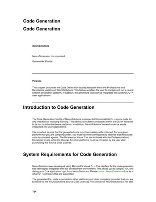
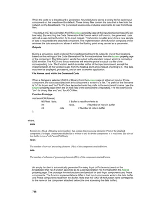
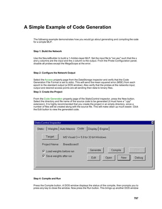
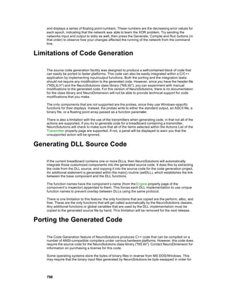

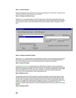


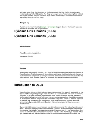
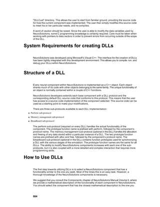


![Step 3: Edit the Activation Component
Click the Edit button to bring up the source code for the DLL. The implementation of the
performLinearAxon function looks like this:
__declspec(dllexport) void performLinearAxon(
DLLData *instance, // Pointer to instance data (may be NULL)
NSFloat *data, // Pointer to the layer of processing elements (PEs)
int rows, // Number of rows of PEs in the layer
int cols, // Number of columns of PEs in the layer
NSFloat *bias, // Pointer to the layer's bias vector, one for each PE
NSFloat beta // Slope gain scalar, same for all PEs
)
{
int i, length=rows*cols;
for (i=0; i<length; i++)
data[i] = beta*data[i] + bias[i];
}
which simply multiplies the input data by a constant and adds a bias (implementing a linear input-
output map). To change the transfer function to a hyperbolic tangent, you need to edit the code as
follows:
__declspec(dllexport) void performLinearAxon(
DLLData *instance, // Pointer to instance data (may be NULL)
NSFloat *data, // Pointer to the layer of processing elements (PEs)
int rows, // Number of rows of PEs in the layer
int cols, // Number of columns of PEs in the layer
NSFloat *bias, // Pointer to the layer's bias vector, one for each PE
NSFloat beta // Slope gain scalar, same for all PEs
)
{
int i, length=rows*cols;
for (i=0; i<length; i++)
data[i] = (float)tanh(beta*data[i] + bias[i]);
}
The transfer function of the new component will be now the hyperbolic function of the input plus the
bias, implementing the tanh static nonlinearity. Save your changes and return to NeuroSolutions.
Step 4: Edit the Backprop Component
If we want to use this new component in a network that is trained with backpropagation, we also
have to create the corresponding backpropagation component. To implement this modification, you
need to Edit the code of the BackLinearAxon by selecting the BackLinearAxon, clicking on the Edit
button to edit the file bkMyTanh, and replacing:
error[i] *= beta;
with:
error[i] *= beta*(1.0f - data[i]*data[i]);
Step 5: Link your new Components
807](https://image.slidesharecdn.com/neurosolutionshelp-090922003656-phpapp01/85/NeuroDimension-Neuro-Solutions-HELP-807-320.jpg)
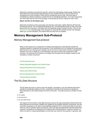
![defined data structures cannot be supported by NeuroSolutions, so you will have to write the code
associated with this data. Next we present the general DLL data structure.
Data Structure
typedef struct {
NSFloat *data;
int length;
} DLLWeights;
typedef struct {
char parameters[5][3][64];
char parameterNames[5][3][64];
} DLLParameters;
typedef struct {
DLLWeights *weights;
DLLParameters *parameters;
void *userData;
} DLLData;
The data variables that are available to the user are:
data
Pointer to a floating point array containing the user-defined weights. This pointer is accessed by
calling the getWeights function defined within "NSDLL.H". Note that the memory is allocated and
freed within NeuroSolutions.
length
The number of weights stored within data. This number is specified when the weights are allocated
(by calling the setWeights function defined within "NSDLL.H").
parameters
Storage for 15 parameter values -- 5 rows and 3 columns. The values are set using the
setBoolParameter, setIntParameter, setFloatParameter, and setStringParameter functions defined
within "NSDLL.H". These values are converted if needed and stored as strings. The parameter
values are retrieved using the getBoolParameter, getIntParameter, getFloatParameter, and
getStringParameter functions.
parameterNames
Storage for 15 parameter names, corresponding to the 15 parameter values. These are used as
labels within the DLL property page of the Inspector window.
weights
Pointer to the DLLWeights structure that holds the user-defined weights. This structure is allocated
by calling the setWeights function defined within "NSDLL.H"
parameters
Pointer to the DLLParameters structure that holds the user-defined parameters. This structure is
allocated during the first call to the setParameterName function defined with in "NSDLL.H".
userData
809](https://image.slidesharecdn.com/neurosolutionshelp-090922003656-phpapp01/85/NeuroDimension-Neuro-Solutions-HELP-809-320.jpg)
![Pointer to a user-defined block of data. The memory is allocated and freed by the user, and the
pointer is updated by calling the setUserData function defined within "NSDLL.H".
See Also
Adding Adaptable Weights to the Instance Data
There may be times when you want to add an adaptable weight vector to a component that already
has a set of adaptable weights . Recall that a TanhAxon has a bias vector (because it is a subclass
of BiasAxon), which may be adapted during learning. The beta term (the slope of the tanh function)
is not adaptable and is the same for all PEs. Suppose that you want to have a unique beta for each
PE and that these terms should be adaptable. This is a case where an instance weight vector is
needed (see Adjustable Transfer Function Slope DLL Example).
An instance weight vector is defined by making a call to the setWeights function within the alloc
function of the DLL:
__declspec(dllexport) DLLData *allocLinearAxon(
DLLData* oldInstance, // Pointer to the last instance if reallocating
int rows, // Number of rows of PEs in the layer
int cols // Number of columns of PEs in the layer
)
{
DLLData *instance = allocDLLInstance(oldInstance);
setWeights(instance, rows*cols);
return instance;
}
The setWeights function simply allocates a vector of weights of the specified size, and inserts it
within the instance of DLLData. The memory for the weights is automatically freed when the
instance is freed (by calling freeDLLInstance from the freeInstance function of the DLL). Note that
the implementation of all DLL functions can be found within the "NSDll.h" header file.
The weights are automatically adapted the same way as the base component’s weights . The
attached Backprop component will compute the gradients and sensitivities for both sets of weights,
and the Gradient Search component will update all of the weights based on the computed
gradients. Note that adaptable instance weights only apply to members of the Axon and Synapse
families.
If an Axon or Synapse has a vector of adaptable weights, then the component’s backpropagation
dual must have a corresponding set of gradients. These gradients are treated as weights in an
identical manner to that of the activation dual.
Within the perform function of a DLL, you obtain a pointer to the weight vector by using the
getWeights function call:
NSFloat *beta = getWeights(instance);
From there you access the individual weights by indexing into the array (e.g., beta[i]).
810](https://image.slidesharecdn.com/neurosolutionshelp-090922003656-phpapp01/85/NeuroDimension-Neuro-Solutions-HELP-810-320.jpg)

![If the force flag is set to FALSE, then the parameter is only assigned if the current setting is
undefined (blank). Otherwise, the parameter is always set to the specified value. This flag should
always be set for FALSE for parameter initialization in order to avoid overwriting a previously
specified value.
Here is an example of how a parameter’s value is retrieved and used:
int i, length=rows*cols;
NSFloat amplitude = getFloatParameter(instance, 1, 1);
for (i=0; i<length; i++)
data[i] = (NSFloat)amplitude*data[i];
The function prototypes for retrieving the parameter values are similar to those used to set them:
int getIntParameter(DLLData *instance, int row, int col);
BOOL getBoolParameter(DLLData *instance, int row, int col);
NSFloat getFloatParameter(DLLData *instance, int row, int col);
char *getStringParameter(DLLData *instance, int row, int col);
See Also
Adding User-Defined Data
During the definition of your new components you may have necessity to define instance variables
and data. NeuroSolutions will maintain a pointer to this data for each instance of the DLL
component. You are responsible for allocating this data during the alloc sub-protocol, freeing it
during the free sub-protocol, and interpreting it during the perform sub-protocol. NeuroSolutions
only maintains a single pointer, so all user-defined data must be organized within a single data
structure.
For example, if you wanted each instance of your component to contain an integer variable called
length and a floating point array called dataArray, then you should define the following data
structure within your DLL:
typedef struct {
int length;
float *dataArray;
} MyData;
Memory Management of Instance Data
Allocation
An instance of a DLL is allocated when the DLL is first loaded, and it is reallocated whenever the
component itself is reallocated (e.g., the number of PEs change), or the instance data is reallocated
due to a change in a specially-tagged instance parameter. (Note that the instance parameter is
tagged by setting realloc=TRUE when calling the setParameterName function.) Whenever a DLL
instance is allocated or reallocated, the DLL’s instance allocation function is called.
812](https://image.slidesharecdn.com/neurosolutionshelp-090922003656-phpapp01/85/NeuroDimension-Neuro-Solutions-HELP-812-320.jpg)
![See Also
Creating Global Variables
A very powerful concept that is supported in the DLLs is the global variable. Global variables allow
several component DLLs to share the same memory. The user must declare global variables at the
top of the DLL. When there are several components using the same DLL, the system only loads the
DLL into memory once. In other words, all of those components share the same memory space
when accessing the DLL. For this reason, any g lobal variables that are declared within the DLL are
global to all instances using the DLL.
Example
Stamp two TanhAxons on a blank breadboard and bring up the inspector for one of them. From the
Engine property page click the New button and enter "MyAxon" as the DLL name. Edit the code as
follows:
NSFloat myBeta = 0.01f;
__declspec(dllexport) void performLinearAxon(
DLLData *instance, // Pointer to instance data (may be NULL)
NSFloat *data, // Pointer to the layer of processing elements (PEs)
int rows, // Number of rows of PEs in the layer
int cols, // Number of columns of PEs in the layer
NSFloat *bias, // Pointer to the layer's bias vector, one for each PE
NSFloat beta // Slope gain scalar, same for all PEs
)
{
int i, length=rows*cols;
for (i=0; i<length; i++) {
data[i] = (NSFloat)tanh(myBeta*data[i] + bias[i]);
myBeta += 0.01f;
}
}
In this code myBeta is a global variable since it is defined before the perform function. Click the
Compile button to create and load this DLL. Select the other TanhAxon and click the Load button
from the Engine property page. Select the "MyAxon" DLL that you have just compiled. Now both
components are sharing the same DLL. Select the Transfer Function property page to observe the
effect of the global variable. Note that NeuroSolutions computes this graph by making consecutive
calls to performLinearAxon, thus the slope of the hyperbolic tangent function (myBeta) increases
with every point that is plotted. Now view the Transfer Function property page of the other
TanhAxon. It plotted the function based on the value of myBeta computed by the first TanhAxon.
Switch back and forth between the two components to observe the increasing slope of the transfer
function.
If these two DLL instances were placed in a network, then the slope would increase twice for each
sample of data run through the network because each instantiated object would be incrementing
the same variable.
814](https://image.slidesharecdn.com/neurosolutionshelp-090922003656-phpapp01/85/NeuroDimension-Neuro-Solutions-HELP-814-320.jpg)
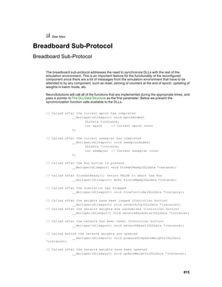


![All three DLLs have very similar implementations, so only the code for hyperbolic tangent will be
shown here. Refer to the sample source code for the implementations of the other two.
The implementation for the activation DLL ("adjtana") is as follows:
void performBiasAxon(
DLLData *instance, // Pointer to instance data
NSFloat *data, // Pointer to the layer of processing elements (PEs)
int rows, // Number of rows of PEs in the layer
int cols, // Number of columns of PEs in the layer
NSFloat *bias // Pointer to the layer's bias vector, one for each PE
)
{
int i, length=rows*cols;
NSFloat *beta = getWeights(instance);
for (i=0; i<length; i++) {
if (beta[i] < 0.5f)
beta[i] = 0.5f;
data[i] = (NSFloat)tanh(beta[i]*data[i] + bias[i]);
}
}
Compare this with the implementation for the base component (TanhAxon):
int i, length=rows*cols;
for (i=0; i<length; i++)
data[i] = (NSFloat)tanh(beta*data[i] + bias[i]);
The weight vector is stored within the DLLData structure and the pointer is obtained with the
getWeights function. The weights are accessed by indexing the floating point array.
Note that there is minimum value forced on each beta term. When the network is reset, the weights
are randomized to a value between -1 and 1. The beta term must be greater than zero. The higher
the beta, the steeper the slope and the more discriminating the function becomes. A value of 0.5
was chosen as a minimum value for this starting point. Most often, the network will adapt to a
higher value.
The implementation for the backpropagation DLL ("bkadjtan") is as follows:
void performBackBiasAxon(
DLLData *instance, // Pointer to instance data
DLLData *dualInstance, // Pointer to the forward axons instance data
NSFloat *data, // Pointer to the layer of processing elements
(PEs)
int rows, // Number of rows of PEs in the layer
int cols, // Number of columns of PEs in the layer
NSFloat *error, // Pointer to the sensitivity vector
NSFloat *gradient // Pointer to the bias gradient vector
)
{
int i,length=rows*cols;
NSFloat *beta = getWeights(dualInstance);
NSFloat *betaGradient = getWeights(instance);
for (i=0; i<length; i++) {
error[i] *= beta[i]*(1.0f - data[i]*data[i] + 0.1f);
if (gradient)
818](https://image.slidesharecdn.com/neurosolutionshelp-090922003656-phpapp01/85/NeuroDimension-Neuro-Solutions-HELP-818-320.jpg)
![gradient[i] += error[i];
if (betaGradient)
betaGradient[i] += error[i]*data[i];
}
}
Compare this with the implementation for the base component (BackTanhAxon):
int i, length=rows*cols;
for (i=0; i<length; i++) {
error[i] *= beta*(1.0f - data[i]*data[i] + 0.1f);
if (gradient)
gradient[i] += error[i];
}
The only differences are that the beta term is unique to each PE and that the gradient information
for the beta vector is computed along with the gradient information for the Axon’s weights.
See Also
TanhAxon with Gain DLL Example
Within the "DLLCUST/LinAxon" directory is a DLL example entitled "gaintanh" and its
corresponding backprop dual "bkgainta". This DLL implements a specialized version of the
TanhAxon to demonstrate the use of instance parameters .
The transfer function of the base TanhAxon produces an output that ranges from -1 to 1. There are
cases when you may want to have the output scaled to match that of the original data. This would
be one use for a TanhAxon component that is enhanced with a gain factor.
The gain parameter is stored within the instance data of the activation component (the TanhAxon).
It is initialized within the allocLinearAxon function as follows:
DLLData *allocLinearAxon(
DLLData *oldInstance, // Pointer to the last instance if reallocating
int rows, // Number of rows of PEs in the layer
int cols // Number of columns of PEs in the layer
)
{
DLLData *instance = allocDLLInstance(oldInstance);
setParameterName(instance, 2, 1, "Gain");
setFloatParameter(instance, 2, 1, 1.0f, FALSE);
return instance;
}
The two function calls set the label on the inspecto r to "Gain" and set the default value to 1.0. The
call to setParameterName must occur before the call to setFloatParameter in order to allocate
memory for the parameters. Note that since the parameters are stored with the instance data, that
memory is auto matically freed when the freeDllInstance function is called.
819](https://image.slidesharecdn.com/neurosolutionshelp-090922003656-phpapp01/85/NeuroDimension-Neuro-Solutions-HELP-819-320.jpg)
![The implementation for the activation DLL ("gaintanh") is as follows:
void performLinearAxon(
DLLData *instance, // Pointer to instance data
NSFloat *data, // Pointer to the layer of processing elements (PEs)
int rows, // Number of rows of PEs in the layer
int cols, // Number of columns of PEs in the layer
NSFloat *bias, // Pointer to the layer's bias vector, one for each PE
NSFloat beta // Slope gain scalar, same for all PEs
)
{
int i, length=rows*cols;
NSFloat gain = getFloatParameter(instance, 2, 1);
for (i=0; i<length; i++)
data[i] = (NSFloat)gain*tanh(beta*data[i] + bias[i]);
}
Compare this with the implementation for the base component (TanhAxon):
int i, length=rows*cols;
for (i=0; i<length; i++)
data[i] = (NSFloat)tanh(beta*data[i] + bias[i]);
The gain parameter is stored within the DLLData structure and the value is obtained with the
getFloatParameter function. The activation function is simply multiplied by this parameter to
produce the scaled result.
The implementation for the backpropagation DLL ("bkgainta") is as follows:
void performBackLinearAxon(
DLLData *instance, // Pointer to instance data
DLLData *dualInstance, // Pointer to the forward axons instance data
NSFloat *data, // Pointer to the layer of processing elements
(PEs)
int rows, // Number of rows of PEs in the layer
int cols, // Number of columns of PEs in the layer
NSFloat *error, // Pointer to the sensitivity vector
NSFloat *gradient, // Pointer to the bias gradient vector
NSFloat beta // Slope gain scalar, same for all PEs
)
{
int i, length=rows*cols;
NSFloat gain = getFloatParameter(dualInstance, 2, 1);
for (i=0; i<length; i++) {
error[i] *= gain*beta*(1.0f - data[i]*data[i] + 0.1f);
if (gradient)
gradient[i] += error[i];
}
}
Compare this with the implementation for the base component (BackTanhAxon):
int i, length=rows*cols;
for (i=0; i<length; i++) {
error[i] *= beta*(1.0f - data[i]*data[i] + 0.1f);
820](https://image.slidesharecdn.com/neurosolutionshelp-090922003656-phpapp01/85/NeuroDimension-Neuro-Solutions-HELP-820-320.jpg)
![if (gradient)
gradient[i] += error[i];
}
The backprop component does not need to store its own gain parameter. Instead, it retrieves it
from the activation dual component by passing the dualInstance pointer to the getFloatParameter
function.
See Also
Synapse
Subset FullSynapse DLL Example
Within the "DLLCUST/Synapse" directory is a DLL example entitled "subsyn" and its corresponding
backprop DLL, "bksubsyn". These DLLs implement a specialized version of the Synapse
component to demonstrate connectivity customization using instance parameters .
When connecting two Axons of differing size together using the base Synapse component, all N
PEs of the smaller Axon are connected to the first N PEs of the larger Axon. This DLL provides
more flexibility by letting the user specify a subset of PEs from one Axon that is to be connected to
the other Axon.
The user has three parameters to work with from the DLL property page of the inspector. The Input
parameter specifies which Axon to select the segment of PEs from -- the input (Input=TRUE) or
output (Input=FALSE). The segment begins with the Start PE and ends with the Start+Length-1 PE.
These PEs are connected to the other Axon in order starting with PE 0.
DLLData *allocSynapse(
DLLData *oldInstance, // Pointer to the last instance if reallocating
int inRows, // Number of rows of PEs in the input layer
int inCols, // Number of columns of PEs in the input layer
int outRows, // Number of rows of PEs in the output layer
int outCols // Number of columns of PEs in the output layer
)
{
BOOL subInput;
int maxLength, start, length;
DLLData *instance = allocDLLInstance(oldInstance);
setParameterName(instance, 1, 1, "Input", TRUE);
setBoolParameter(instance, 1, 1, TRUE, FALSE);
setParameterName(instance, 2, 1, "Start", TRUE);
setIntParameter(instance, 2, 1, 0, FALSE);
setParameterName(instance, 3, 1, "Length", TRUE);
setIntParameter(instance, 3, 1, 1, FALSE);
subInput = getBoolParameter(instance, 1, 1);
maxLength = subInput? inRows*inCols: outRows*outCols;
start = getIntParameter(instance, 2, 1);
if (inRows && inCols && outRows && outCols) {
if (start >= maxLength)
start = maxLength-1;
821](https://image.slidesharecdn.com/neurosolutionshelp-090922003656-phpapp01/85/NeuroDimension-Neuro-Solutions-HELP-821-320.jpg)
![length = getIntParameter(instance, 3, 1);
if (start+length > maxLength)
length = maxLength-start;
if (!subInput)
if (length > inRows*inCols)
length = inRows*inCols;
} else
start = length = 0;
setBoolParameter(instance, 1, 1, subInput, TRUE);
setIntParameter(instance, 2, 1, start, TRUE);
setIntParameter(instance, 3, 1, length, TRUE);
return instance;
}
The call to freeDLLInstance handles the freeing of the instance parameters:
void freeInstance(DLLData *instance)
{
freeDLLInstance(instance);
}
The implementation for the activation DLL ("subsyn") is as follows:
void performSynapse(
DLLData *instance, // Pointer to instance data
NSFloat *input, // Pointer to the input layer of PEs
int inRows, // Number of rows of PEs in the input layer
int inCols, // Number of columns of PEs in the input layer
NSFloat *output, // Pointer to the output layer
int outRows, // Number of rows of PEs in the output layer
int outCols // Number of columns of PEs in the output layer
)
{
BOOL subInput = getBoolParameter(instance, 1, 1);
int i,
inCount = subInput? getIntParameter(instance, 3, 1): inRows*inCols,
outCount = !subInput? getIntParameter(instance, 3, 1):
outRows*outCols,
start = getIntParameter(instance, 2, 1),
count = inCount<outCount? inCount: outCount;
if (subInput)
for (i=0; i<count; i++)
output[i] += input[i+start];
else
for (i=0; i<count; i++)
output[i+start] += input[i];
}
Compare this with the implementation for the base component (Synapse):
int i,
inCount=inRows*inCols,
outCount=outRows*outCols,
count = inCount<outCount? inCount: outCount;
822](https://image.slidesharecdn.com/neurosolutionshelp-090922003656-phpapp01/85/NeuroDimension-Neuro-Solutions-HELP-822-320.jpg)
![for (i=0; i<count; i++)
output[i] += input[i];
The implementation for the backpropagation DLL ("bksubsyn") is as follows:
void performBackSynapse(
DLLData *instance, // Pointer to instance data
DLLData *dualInstance // Pointer to the forward synapses instance data
NSFloat *errorIn, // Pointer to the input error layer of PEs
int inRows, // Number of rows of PEs in the input layer
int inCols, // Number of columns of PEs in the input layer
NSFloat *errorOut, // Pointer to the output error layer
int outRows, // Number of rows of PEs in the output layer
int outCols, // Number of columns of PEs in the output layer
NSFloat *input // Pointer to output layer of forward synapse
)
{
BOOL subInput = getBoolParameter(dualInstance, 1, 1);
int i,
inCount = !subInput? getIntParameter(dualInstance, 3, 1):
inRows*inCols,
outCount = subInput? getIntParameter(dualInstance, 3, 1):
outRows*outCols,
start = getIntParameter(dualInstance, 2, 1),
count = inCount<outCount? inCount: outCount;
if (subInput)
for (i=0; i<count; i++)
errorOut[i+start] += errorIn[i];
else
for (i=0; i<count; i++)
errorOut[i] += errorIn[i+start];
}
Compare this with the implementation for the base component (BackSynapse):
int i,
inCount=inRows*inCols,
outCount=outRows*outCols,
count=inCount<outCount? inCount: outCount;
for (i=0; i<count; i++)
errorOut[i] += errorIn[i];
See Also
Locally-Connected Synapse DLL Example
Within the "DLLCUST/Synapse" directory is a DLL example entitled "localsyn" and its
corresponding backprop DLL, "bklocals". These DLLs implement a specialized version of the
Synapse component to demonstrate connectivity customization using instance weights .
823](https://image.slidesharecdn.com/neurosolutionshelp-090922003656-phpapp01/85/NeuroDimension-Neuro-Solutions-HELP-823-320.jpg)
![colSize = (int)inCols/outCols,
colRemainder = inCols-outCols*colSize,
rowSize = (int)inRows/outRows,
rowRemainder = inRows-outRows*rowSize;
NSFloat *weights = getWeights(instance);
for (i=0; i<outRows; i++)
for (j=0; j<outCols; j++) {
startRow = rowSize*i;
if (i == outRows-1)
stopRow = inRows;
else
stopRow = rowSize*(i+1);
startCol = colSize*j;
if (j == outCols-1)
stopCol = inCols;
else
stopCol = colSize*(j+1);
for (k=startRow; k<stopRow; k++)
for (l=startCol; l<stopCol; l++)
out(i,j) += *weights++ * in(k,l);
}
}
Compare this with the implementation for the base component (Synapse):
int i,
inCount=inRows*inCols,
outCount=outRows*outCols,
count = inCount<outCount? inCount: outCount;
for (i=0; i<count; i++)
output[i] += input[i];
The implementation for the backpropagation DLL ("bklocals") is as follows:
void performBackSynapse(
DLLData *instance, // Pointer to instance data
DLLData *dualInstance // Pointer to the forward synapses instance data
NSFloat *errorIn, // Pointer to the input error layer of PEs
int inRows, // Number of rows of PEs in the input layer
int inCols, // Number of columns of PEs in the input layer
NSFloat *errorOut, // Pointer to the output error layer
int outRows, // Number of rows of PEs in the output layer
int outCols, // Number of columns of PEs in the output layer
NSFloat *input // Pointer to output layer of forward synapse
)
{
int i, j, k, l, startRow, stopRow, startCol, stopCol,
colSize = (int)outCols/inCols,
colRemainder = outCols-inCols*colSize,
rowSize = (int)outRows/inRows,
rowRemainder = outRows-inRows*rowSize;
NSFloat *weights = getWeights(dualInstance);
NSFloat *gradients = getWeights(instance);
for (i=0; i<inRows; i++)
for (j=0; j<inCols; j++) {
825](https://image.slidesharecdn.com/neurosolutionshelp-090922003656-phpapp01/85/NeuroDimension-Neuro-Solutions-HELP-825-320.jpg)
![startRow = rowSize*i;
if (i == inRows-1)
stopRow = outRows;
else
stopRow = rowSize*(i+1);
startCol = colSize*j;
if (j == inCols-1)
stopCol = outCols;
else
stopCol = colSize*(j+1);
for (k=startRow; k<stopRow; k++)
for (l=startCol; l<stopCol; l++) {
out(k,l) += *weights++ * in(i,j);
*gradients++ += in(i,j) * activity(k,l);
}
}
}
Compare this with the implementation for the base component (BackSynapse):
int i,
inCount=inRows*inCols,
outCount=outRows*outCols,
count=inCount<outCount? inCount: outCount;
for (i=0; i<count; i++)
errorOut[i] += errorIn[i];
See Also
ErrorCriterion
Loser Learn All DLL Example
Within the "DLLCUST/ErrCrit" directory is a DLL example entitled "loserlrn". This DLL implements a
modified version of the L2Criterion. Instead of backpropagating the sensitivities for all output PEs,
this algorithm only passes back the sensitivity data for the PE that has the highest error. The rest of
the sensitivity vector is forced to zero.
NSFloat performCriterion(
DLLData *instance, // Pointer to instance data (may be NULL)
NSFloat *costDerivative, // Pointer to the cost derivative vector,
// i.e. output sensitivity
int rows, // Number of rows of PEs in the layer
int cols, // Number of columns of PEs in the layer
NSFloat *output, // Pointer to the output layer of the network
NSFloat *desired // Pointer to the desired output vector, same
// length as output layer
)
{
int i,maxInt=0,length=rows*cols;
826](https://image.slidesharecdn.com/neurosolutionshelp-090922003656-phpapp01/85/NeuroDimension-Neuro-Solutions-HELP-826-320.jpg)
![NSFloat cost = 0.0f;
for (i=0; i<length; i++) {
costDerivative[i] = desired[i] - output[i];
cost += costDerivative[i]*costDerivative[i];
if (fabs(costDerivative[i]) > fabs(costDerivative[maxInt]))
maxInt = i;
}
for (i=0; i<length; i++)
if (i != maxInt)
costDerivative[i] = 0.0f;
return cost;
}
Compare this with the implementation for the base component (L2Criterion):
int i,length=rows*cols;
NSFloat cost=0.0f;
for (i=0; i<length; i++) {
costDerivative[i] = desired[i] - output[i];
cost += costDerivative[i]*costDerivative[i];
}
return cost;
See Also
GradientSearch
DeltaBarDelta with Limited Step DLL Example
Within the "DLLCUST/DeltaBar" directory is a DLL example entitled "limitdbd". This DLL
implements a modified version of the DeltaBarDelta. The base DeltaBarDelta component has an
adaptive step size. In some cases, this step size may grow too large and make the network
unstable. This DLL uses an instance parameter to allow the user to specify the maximum step size
that any PE can have. This parameter is defined within the allocation function:
DLLData *allocDeltaBarDelta(
DLLData *oldInstance, // Pointer to the last instance if reallocating
int length, // Length of the weight vector
BOOL individual // Indicates whether their is one learning rate for
//all weights (FALSE),
// or each weight has its own learning rate
)
{
DLLData *instance = allocDLLInstance(oldInstance);
setParameterName(instance, 2, 1, "Max Step", TRUE);
setFloatParameter(instance, 2, 1, 0.1f, FALSE);
if (getFloatParameter(instance, 2, 1) < 0)
setFloatParameter(instance, 2, 1, 0.0f, TRUE);
return instance;
}
827](https://image.slidesharecdn.com/neurosolutionshelp-090922003656-phpapp01/85/NeuroDimension-Neuro-Solutions-HELP-827-320.jpg)
![The parameter (stepMax) is then used to limit the step size of each PE:
void performDeltaBarDelta(
DLLData *instance, // Pointer to instance data (may
be NULL)
NSFloat *step, // Pointer to vector of learning
rates for each
// weight
int length, // Length of learning rate
vector
NSFloat momentum, // Momentum rate for all weights
NSFloat *delta, // Last weight Update
NSFloat *gradient, // Gradient vector from backprop
component
NSFloat *smoothedGradient, // Smoothed gradient vector
NSFloat beta, // Multiplicative constant
NSFloat kappa, // Additive constant
NSFloat zeta // Smoothing factor
)
{
int i;
NSFloat stepMax = getFloatParameter(instance, 2, 1);
for (i=0; i<length; i++) {
if (smoothedGradient[i]*gradient[i] > 0)
step[i] += kappa;
else
if (smoothedGradient[i]*gradient[i] < 0)
step[i] -= beta*step[i];
if (step[i] > stepMax)
step[i] = stepMax;
smoothedGradient[i] = (1-zeta)*gradient[i] +
zeta*smoothedGradient[i];
}
}
Compare this with the implementati on for the base component (DeltaBarDelta):
int i;
for (i=0; i<length; i++) {
if (smoothedGradient[i]*gradient[i] > 0)
step[i] += kappa;
else
if (smoothedGradient[i]*gradient[i] < 0)
step[i] -= beta*step[i];
smoothedGradient[i] = (1-zeta)*gradient[i] + zeta*smoothedGradient[i];
}
See Also
828](https://image.slidesharecdn.com/neurosolutionshelp-090922003656-phpapp01/85/NeuroDimension-Neuro-Solutions-HELP-828-320.jpg)
![DeltaBarDelta with Exponential Step DLL Example
Within the "DLLCUST/DeltaBar" directory is a DLL example entitled "expdbd". This DLL further
modifies the DeltaBarDelta with Limited Step example. It simply multiplies kappa by an exponential
term when computing the step sizes.
void performDeltaBarDelta(
DLLData *instance, // Pointer to instance data (may
be NULL)
NSFloat *step, // Pointer to vector of learning
rates for each
// weight
int length, // Length of learning rate
vector
NSFloat momentum, // Momentum rate for all weights
NSFloat *delta, // Last weight Update
NSFloat *gradient, // Gradient vector from backprop
component
NSFloat *smoothedGradient, // Smoothed gradient vector
NSFloat beta, // Multiplicative constant
NSFloat kappa, // Additive constant
NSFloat zeta // Smoothing factor
)
{
int i;
NSFloat gamma = getFloatParameter(instance, 2, 1);
NSFloat stepMax = getFloatParameter(instance, 3, 1);
for (i=0; i<length; i++) {
if (smoothedGradient[i]*gradient[i] > 0)
step[i] += kappa * (NSFloat)exp(-
gamma*fabs(smoothedGradient[i]));
else
if (smoothedGradient[i]*gradient[i] < 0)
step[i] -= beta*step[i];
if (step[i] > stepMax)
step[i] = stepMax;
smoothedGradient[i] = (1-zeta)*gradient[i] +
zeta*smoothedGradient[i];
}
}
See Also
General Input and Postprocessor
Strange Attractor DLL Example
Within the "DLLCUST/PrePost" directory is a DLL example entitled "strange". This DLL implements
a strange attractor using the DLLInput component.
829](https://image.slidesharecdn.com/neurosolutionshelp-090922003656-phpapp01/85/NeuroDimension-Neuro-Solutions-HELP-829-320.jpg)
![A strange attractor is a chaotic system whose path in phase space is fully determined, but never
recurs. The particular attractor implemented by this DLL is represented by the following 3
equations:
x[n+1] = sin(a*y[n]) - z[n]cos(b*x[n])
y[n+1] = z[n]sin(c*x[n]) - cos(d*y[n])
z[n+1] = sin(x[n])
The user specifies the 4 constants (a, b, c, and d) and the starting point (x[0], y[0], and z[0]). The
system state described by the 3-D point and the constants will ultimately converge to the attractor
after enough iterations.
The implementation of the strange attractor requires the use of 7 user-defined parameters (the 4
constants and the starting point) and 3 instance variables (the previous x, y, and z).
void performInput(
DLLData *instance, // Pointer to instance data (may be NULL)
NSFloat *data, // Pointer to the data
int rows, // Number of rows of data
int cols // Number of cols of data
)
{
int i;
NSFloat a = getFloatParameter(instance, 1, 1);
NSFloat b = getFloatParameter(instance, 2, 1);
NSFloat c = getFloatParameter(instance, 3, 1);
NSFloat d = getFloatParameter(instance, 4, 1);
NSFloat *lastResult = (NSFloat*)getUserData(instance);
data[0] = (NSFloat)(sin(a*lastResult[1]) -
lastResult[2]*cos(b*lastResult[0]));
if (rows*cols > 1) {
data[1] = (NSFloat)(lastResult[2]*sin(c*lastResult[0]) -
cos(d*lastResult[1]));
if (rows*cols > 2) {
data[2] = (NSFloat)sin(lastResult[0]);
lastResult[2] = data[2];
}
lastResult[1] = data[1];
}
lastResult[0] = data[0];
}
void networkReset(
DLLData *instance // Pointer to instance data (may be NULL)
)
{
int i;
NSFloat Xo = getFloatParameter(instance, 1, 2);
NSFloat Yo = getFloatParameter(instance, 2, 2);
NSFloat Zo = getFloatParameter(instance, 3, 2);
NSFloat *lastData = (NSFloat*)getUserData(instance);
lastData[0] = Xo;
830](https://image.slidesharecdn.com/neurosolutionshelp-090922003656-phpapp01/85/NeuroDimension-Neuro-Solutions-HELP-830-320.jpg)
![lastData[1] = Yo;
lastData[2] = Zo;
}
DLLData *allocInput(
DLLData *oldInstance, // Pointer to the last instance if reallocating
int rows, // Number of rows of data
int cols // Number of cols of data
)
{
DLLData *instance = allocDLLInstance(oldInstance);
setUserData(instance, calloc(3, sizeof(NSFloat)));
setParameterName(instance, 1, 1, "a", FALSE);
setFloatParameter(instance, 1, 1, 2.24f, FALSE);
setParameterName(instance, 2, 1, "b", FALSE);
setFloatParameter(instance, 2, 1, 0.43f, FALSE);
setParameterName(instance, 3, 1, "c", FALSE);
setFloatParameter(instance, 3, 1, -0.65f, FALSE);
setParameterName(instance, 4, 1, "d", FALSE);
setFloatParameter(instance, 4, 1, -2.43f, FALSE);
setParameterName(instance, 1, 2, "Xo", FALSE);
setFloatParameter(instance, 1, 2, 0.0f, FALSE);
setParameterName(instance, 2, 2, "Yo", FALSE);
setFloatParameter(instance, 2, 2, 0.0f, FALSE);
setParameterName(instance, 3, 2, "Zo", FALSE);
setFloatParameter(instance, 3, 2, 0.0f, FALSE);
networkReset(instance);
return instance;
}
void freeInput(DLLData *instance)
{
if (getUserData(instance))
free(getUserData(instance));
freeDLLInstance(instance);
}
See Also
Logistic Map DLL Example
Within the "DLLCUST/PrePost" directory is a DLL example entitled "logistic". This DLL implements
a logistic map using the DLLInput component.
This logistic map is a simple difference equation that produces widely varying time series (constant
periodic, quasi-periodic, and chaotic) depending upon the value of the parameter R:
R=0.8 - Signal decays to 0
R=2.9 - Alternating decay to a value greater than 0
831](https://image.slidesharecdn.com/neurosolutionshelp-090922003656-phpapp01/85/NeuroDimension-Neuro-Solutions-HELP-831-320.jpg)
![R=3.2 - Cycle of period 2
R=3.5 - Cycle of period 4
R>4 - Chaos
The user specifies the value of R and the initial value of the series (seed). The implementation
requires the use of 2 user-defined parameters and an instance data structure that stores the result
from the last computation.
typedef struct {
NSFloat *data;
int length;
} ResultData;
void performInput(
DLLData *instance, // Pointer to instance data (may be NULL)
NSFloat *data, // Pointer to the data
int rows, // Number of rows of data
int cols // Number of cols of data
)
{
int i;
NSFloat constant = getFloatParameter(instance, 2, 1);
ResultData *results = (ResultData*)getUserData(instance);
for (i=0; i<results->length; i++)
data[i] = results->data[i] = constant * results->data[i] *
(1 - results->data[i]);
}
void networkReset(
DLLData *instance // Pointer to instance data (may be NULL)
)
{
int i;
NSFloat seed = getFloatParameter(instance, 3, 1);
ResultData *results = (ResultData*)getUserData(instance);
for (i=0; i<results->length; i++)
results->data[i] = seed;
}
DLLData *allocInput(
DLLData *oldInstance, // Pointer to the last instance if reallocating
int rows, // Number of rows of data
int cols // Number of cols of data
)
{
DLLData *instance = allocDLLInstance(oldInstance);
ResultData *results = calloc(1,sizeof(ResultData));
results->length = rows*cols;
results->data = calloc(results->length, sizeof(NSFloat));
setUserData(instance, results);
setParameterName(instance, 2, 1, "Constant", FALSE);
setFloatParameter(instance, 2, 1, 4.0f, FALSE);
setParameterName(instance, 3, 1, "Seed", FALSE);
832](https://image.slidesharecdn.com/neurosolutionshelp-090922003656-phpapp01/85/NeuroDimension-Neuro-Solutions-HELP-832-320.jpg)
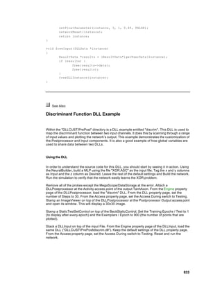
![Discriminant function of the XOR problem
The corners of this graph represent the input data. As expected, the lower-left (-1,-1) and upper-
right (1,1) corners have an output of 0, and the other to two corners have an output of 1. The plot
shows how the network responds to every combination of values in between (in increments of
0.066667).
Functions used by the DLLPostprocessor
The DLLPostprocessor has two parameters defined by the user. The Plot Channel specifies which
PE to use as the output. The number of Steps specifies the resolution of the function. Note that the
number of output channels is Steps squared.
#define matrix(i,j) output[j+(i)*buffer.steps]
typedef struct {
int steps;
int currentX, currentY;
int xChannel, yChannel;
int plotChannel;
NSFloat minX, maxX;
NSFloat minY, maxY;
} BufferData;
834](https://image.slidesharecdn.com/neurosolutionshelp-090922003656-phpapp01/85/NeuroDimension-Neuro-Solutions-HELP-834-320.jpg)
![BufferData buffer = {0, 0, 0, 0, 0, 0, 0.0f, 0.0f, 0.0f, 0.0f};
BOOL performPrePost(
DLLData *instance, // Pointer to instance data (may be NULL)
NSFloat *input, // Pointer to the input data
NSFloat *output, // Pointer to the output data
int rows, // Number of rows of data
int cols, // Number of cols of data
BOOL preprocessor // Flag to indicate whether this is a preprocessor
// or postprocessor
)
{
matrix(buffer.currentX++, buffer.currentY) = input[buffer.plotChannel];
if (buffer.currentX >= buffer.steps) {
buffer.currentX = 0;
if (++buffer.currentY >= buffer.steps) {
buffer.currentY = 0;
return TRUE;
}
}
return FALSE; // Return whether to inject this sample or to call
// performPrePost with another sample
}
void networkReset(
DLLData *instance // Pointer to instance data (may be NULL)
)
{
buffer.currentX = 0;
buffer.currentY = 0;
}
DLLData *allocPrePost(
DLLData *oldInstance, // Pointer to the last instance if reallocating
int *rows, // Number of rows of data attached above -- can
be
// changed. The default is the number of rows
// attached below.
int *cols, // Number of cols of data attached above -- can
be
// changed. The default is the number of cols
// attached below.
BOOL preprocessor // Flag to indicate whether this is a
preprocessor
// or postprocessor
)
{
DLLData *instance = allocDLLInstance(oldInstance);
if (preprocessor)
MessageBox(NULL,
"Confusion matrix should only be used as a postprocessor",
"Warning", MB_OK);
setParameterName(instance, 2, 1, "Steps", TRUE);
setIntParameter(instance, 2, 1, 10, FALSE);
setParameterName(instance, 3, 1, "Plot Channel", TRUE);
setIntParameter(instance, 3, 1, 0, FALSE);
835](https://image.slidesharecdn.com/neurosolutionshelp-090922003656-phpapp01/85/NeuroDimension-Neuro-Solutions-HELP-835-320.jpg)
![buffer.steps = getIntParameter(instance, 2, 1);
buffer.plotChannel = getIntParameter(instance, 3, 1);
if (buffer.steps < 2)
buffer.steps = 2;
if (buffer.plotChannel >= *rows * *cols)
buffer.plotChannel = *rows * *cols - 1;
setIntParameter(instance, 2, 1, buffer.steps, TRUE);
setIntParameter(instance, 3, 1, buffer.plotChannel, TRUE);
*rows = *cols = buffer.steps;
networkReset(instance);
return instance;
}
void freePrePost(DLLData *instance)
{
freeDLLInstance(instance);
}
Functions used by the DLLInput
The DLLInput has six parameters defined by the user. The X Channel and Y Channel parameters
specify which two PEs to use as the function’s input. The Min X, Min Y, Max X and Max Y
parameters specify the range of values to scan across. Note that the resolution of the scan is
defined by the Steps parameter of the DLLPostprocessor.
void performInput(
DLLData *instance, // Pointer to instance data (may be NULL)
NSFloat *data, // Pointer to the data
int rows, // Number of rows of data
int cols // Number of cols of data
)
{
data[buffer.xChannel] = buffer.minX +
buffer.currentX*(buffer.maxX-
buffer.minX)/(buffer.steps-1);
data[buffer.yChannel] = buffer.minY +
buffer.currentY*(buffer.maxY-
buffer.minY)/(buffer.steps-1);
}
DLLData *allocInput(
DLLData *oldInstance, // Pointer to the last instance if reallocating
int rows, // Number of rows of data
int cols // Number of cols of data
)
{
DLLData *instance = allocDLLInstance(oldInstance);
setParameterName(instance, 2, 0, "X Channel", TRUE);
setIntParameter(instance, 2, 0, 0, FALSE);
setParameterName(instance, 2, 1, "Min X", TRUE);
setFloatParameter(instance, 2, 1, -1.0f, FALSE);
setParameterName(instance, 2, 2, "Max X", TRUE);
setFloatParameter(instance, 2, 2, 1.0f, FALSE);
setParameterName(instance, 3, 0, "Y Channel", TRUE);
setIntParameter(instance, 3, 0, 1, FALSE);
setParameterName(instance, 3, 1, "Min Y", TRUE);
836](https://image.slidesharecdn.com/neurosolutionshelp-090922003656-phpapp01/85/NeuroDimension-Neuro-Solutions-HELP-836-320.jpg)


![n Run the network. The displayed output data should be denormalized to match the desired output data.
How the DLL is Implemented
This DLL has 2 instance parameters. The Gain specifies the multiplicative constant and the Offset
specifies the additive constant.
BOOL performPrePost(
DLLData *instance, // Pointer to instance data (may be NULL)
NSFloat *input // Pointer to the input data
NSFloat *output, // Pointer to the output data
int rows, // Number of rows of data
int cols, // Number of cols of data
BOOL preprocessor // Flag to indicate whether this is a preprocessor or
postprocessor
)
{
int i, length=rows*cols;
float gain = getFloatParameter(instance, 2, 1);
float offset = getFloatParameter(instance, 3, 1);
for (i=0; i<length; i++)
output[i] += gain*(input[i] + offset);
return TRUE;
}
DLLData *allocPrePost(
DLLData *oldInstance, // Pointer to the last instance if reallocating
int *rows, // Number of rows of data attached above -- can be
// changed. The default is the number of rows
// attached below.
int *cols, // Number of cols of data attached above -- can be
// changed. The default is the number of cols
// attached below.
BOOL preprocessor // Flag to indicate whether this is a preprocessor
// or postprocessor
)
{
839](https://image.slidesharecdn.com/neurosolutionshelp-090922003656-phpapp01/85/NeuroDimension-Neuro-Solutions-HELP-839-320.jpg)


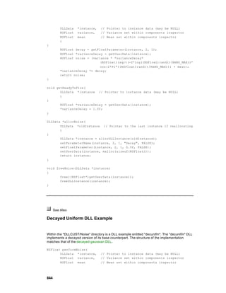
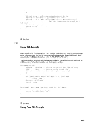

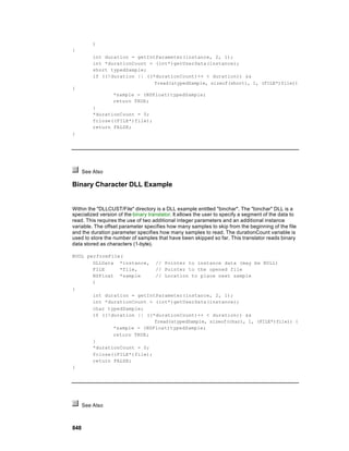
![Preprocessor
Averaging Filter DLL Example
Within the "DLLCUST/PrePost" directory is a DLL examples entitled "average". This DLL
implements an averaging filter, which averages the last N samples of input for each channel and
writes the result to the output for each call to performPrePost. This requires the use of a user-
defined parameter (N) and a vector of instance data (bufferData) to store the past samples.
#definebuffer(i, j) bufferData->data[j+(i)*bufferData->length]
typedef struct {
int length;
NSFloat *data;
} AverageData;
BOOL performPrePost(
DLLData *instance, // Pointer to instance data (may be NULL)
NSFloat *input // Pointer to the input data
NSFloat *output, // Pointer to the output data
int rows, // Number of rows of data
int cols // Number of cols of data
BOOL preprocessor // Flag to indicate preprocessor or postprocessor
)
{
int i, j;
int N = getIntParameter(instance, 2, 1);
AverageData *bufferData = getUserData(instance);
NSFloat result;
for (i=N-1; i>0; i--)
for (j=0; j<bufferData->length; j++)
buffer(i,j) = buffer(i-1,j);
for (j=0; j<bufferData->length; j++)
buffer(0,j) = input[j];
if (!preprocessor) //Zero output buffer if postprocessor (since it is
local)
for (j=0; j<bufferData->length; j++)
output[j] = 0.0f;
for (j=0; j<bufferData->length; j++) {
result = 0.0f;
for (i=0; i<N; i++)
result += buffer(i,j);
output[j] += result/N;
}
return TRUE;
}
void networkReset(
DLLData *instance // Pointer to instance data (may be NULL)
)
{
int i, j;
int N = getIntParameter(instance, 2, 1);
AverageData *bufferData = getUserData(instance);
for (i=0; i<N; i++)
849](https://image.slidesharecdn.com/neurosolutionshelp-090922003656-phpapp01/85/NeuroDimension-Neuro-Solutions-HELP-849-320.jpg)
![for (j=0; j<bufferData->length; j++)
buffer(i,j) = 0.0f;
}
DLLData *allocPrePost(
DLLData *oldInstance, // Pointer to the last instance if reallocating
int *rows, // Number of rows of data attached above -- can be
// changed. The default is the number of rows
// attached below.
int *cols, // Number of cols of data attached above -- can be
// changed. The default is the number of cols
// attached below.
BOOL preprocessor // Flag to indicate whether this is a preprocessor
// or postprocessor
)
{
DLLData *instance = allocDLLInstance(oldInstance);
AverageData *bufferData = calloc(1,sizeof(AverageData));
setParameterName(instance, 2, 1, "N", TRUE);
setIntParameter(instance, 2, 1, 4, FALSE);
bufferData->length = *rows * *cols;
bufferData->data = calloc(bufferData->length*
getIntParameter(instance, 2, 1),
sizeof(NSFloat));
setUserData(instance, bufferData);
return instance;
}
void freePrePost(DLLData *instance)
{
AverageData *bufferData = getUserData(instance);
if (bufferData) {
free(bufferData->data);
free(bufferData);
}
freeDLLInstance(instance);
}
See Also
Decimator Filter DLL Example
Within the "DLLCUST/PrePost" directory is a DLL examples entitled "decimate". This DLL
implements a decimator filter, which reduces the amount of input data by skipping samples. In
order to keep as much of the input information as possible, the samples are averaged together to
produce the output. This is similar to the averaging filter except that the implementation passes the
results to the output one out of every N calls to performPrePost instead of every call. For the other
N-1 calls, it simply stores the input into the bufferData vector. The boolean value returned is used
to specify when to process the output.
#definebuffer(i, j) bufferData->data[j+(i)*bufferData->length]
850](https://image.slidesharecdn.com/neurosolutionshelp-090922003656-phpapp01/85/NeuroDimension-Neuro-Solutions-HELP-850-320.jpg)
![typedef struct {
int length;
NSFloat *data;
} AverageData;
BOOL performPrePost(
DLLData *instance, // Pointer to instance data (may be NULL)
NSFloat *input // Pointer to the input data
NSFloat *output, // Pointer to the output data
int rows, // Number of rows of data
int cols, // Number of cols of data
BOOL preprocessor // Flag to indicate a preprocessor or postprocessor
)
{
int i, j;
int N = getIntParameter(instance, 2, 1);
DecimatorData *bufferData = getUserData(instance);
NSFloat result;
for (i=N-1; i>0; i--)
for (j=0; j<bufferData->length; j++)
buffer(i,j) = buffer(i-1,j);
for (j=0; j<bufferData->length; j++)
buffer(0,j) = input[j];
if (++bufferData->count >= N) {
bufferData->count = 0;
if (!preprocessor) //Zero buffer if postprocessor (since it is
local)
for (j=0; j<bufferData->length; j++)
output[j] = 0.0f;
for (j=0; j<bufferData->length; j++) {
result = 0.0f;
for (i=0; i<N; i++)
result += buffer(i,j);
output[j] = result/N;
}
return TRUE;
}
return FALSE;
}
void networkReset(
DLLData *instance // Pointer to instance data (may be NULL)
)
{
int i, j;
int N = getIntParameter(instance, 2, 1);
DecimatorData *bufferData = getUserData(instance);
for (i=0; i<N; i++)
for (j=0; j<bufferData->length; j++)
buffer(i,j) = 0.0f;
bufferData->count = 0;
}
DLLData *allocPrePost(
DLLData *oldInstance, // Pointer to the last instance if reallocating
int *rows, // Number of rows of data attached above -- can be
851](https://image.slidesharecdn.com/neurosolutionshelp-090922003656-phpapp01/85/NeuroDimension-Neuro-Solutions-HELP-851-320.jpg)
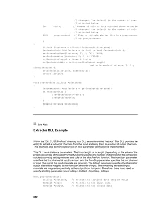
![int rows, // Number of rows of data
int cols, // Number of cols of data
BOOL preprocessor // Flag to indicate preprocessor or postprocessor
)
{
int i;
int fromLength = getIntParameter(instance, 2, 0);
int fromStart = getIntParameter(instance, 2, 1);
int fromStop = getIntParameter(instance, 2, 2);
int toStart = getIntParameter(instance, 3, 1);
if (!preprocessor) //Zero buffer if postprocessor (since it is local)
for (i=0; i<bufferData->length; i++)
output[i] = 0.0f;
for (i=0; i<=fromStop-fromStart; i++)
output[toStart+i] += input[fromStart+i];
return TRUE;
}
DLLData *allocPrePost(
DLLData *oldInstance, // Pointer to the last instance if reallocating
int *rows, // Number of rows of data attached above -- can be
// changed. The default is the number of rows
// attached below.
int *cols, // Number of cols of data attached above -- can be
// changed. The default is the number of cols
// attached below.
BOOL preprocessor // Flag to indicate whether this is a preprocessor
// or postprocessor
)
{
DLLData *instance = allocDLLInstance(oldInstance);
int fromLength, toLength, fromStart, fromStop, toStart, returnMax;
setParameterName(instance, 2, 1, "From Start", TRUE);
setIntParameter(instance, 2, 1, 0, FALSE);
setParameterName(instance, 2, 2, "From Stop", TRUE);
setIntParameter(instance, 2, 2, 0, FALSE);
setParameterName(instance, 3, 1, "To Start", TRUE);
setIntParameter(instance, 3, 1, 0, FALSE);
if (preprocessor) {
setParameterName(instance, 2, 0, "From Length", TRUE);
setIntParameter(instance, 2, 0, 1, FALSE);
returnMax = fromLength = getIntParameter(instance, 2, 0);
toLength = *rows * *cols;
} else {
setParameterName(instance, 2, 0, "To Length", TRUE);
setIntParameter(instance, 2, 0, 1, FALSE);
fromLength = *rows * *cols;
returnMax = toLength = getIntParameter(instance, 2, 0);
}
if (fromLength < 1)
fromLength = 1;
fromStart = getIntParameter(instance, 2, 1);
if (fromStart >= fromLength)
fromStart = fromLength - 1;
fromStop = getIntParameter(instance, 2, 2);
853](https://image.slidesharecdn.com/neurosolutionshelp-090922003656-phpapp01/85/NeuroDimension-Neuro-Solutions-HELP-853-320.jpg)
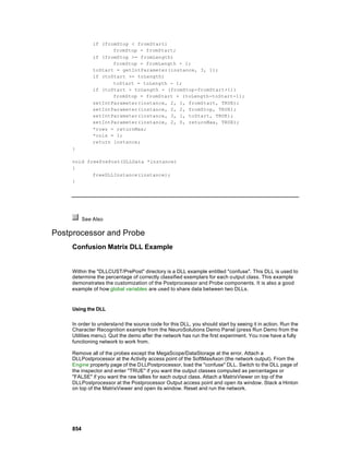

![Confusion Matrix of the Sleep Staging Example
In the first example, the DLLPreprocessor knew which PE was supposed to be active because the
exemplars were ordered. For this example, it is the job of the Probe DLL attached to the desired
output File to communicate with the DLLPreprocessor to tell it the active PE for each exemplar.
This is done by sharing global variables within the same DLL source file.
Functions used by the DLLPostprocessor
#define matrix(i,j) buffer.output[j+i*buffer.length]
typedef struct {
int length;
int currentClass;
int currentOutput;
BOOL report, zero;
BOOL outputProbe;
NSFloat *output;
} BufferData;
BufferData buffer = {0, 0, 0, FALSE, FALSE, FALSE, NULL};
/*****************************************/
/* Activation of Postprocessor component */
__declspec(dllexport) BOOL performPrePost(
DLLData*instance, // Pointer to instance data (may be NULL)
NSFloat*input, // Pointer to the input data
NSFloat*output, // Pointer to the output data
int rows, // Number of rows of data
int cols, // Number of cols of data
BOOL preprocessor // Flag to indicate whether this is a preprocessor
or postprocessor
)
{
int i, j;
NSFloat total;
BOOL percentFlag = getBoolParameter(instance, 1, 1);
buffer.output = output;
856](https://image.slidesharecdn.com/neurosolutionshelp-090922003656-phpapp01/85/NeuroDimension-Neuro-Solutions-HELP-856-320.jpg)
![buffer.currentOutput = 0;
if (buffer.zero) {
for (i=0; i<buffer.length; i++)
for (j=0; j<buffer.length; j++)
matrix(i,j) = 0.0f;
buffer.zero = FALSE;
}
for (i=1; i<buffer.length; i++)
if (input[i] > input[buffer.currentOutput])
buffer.currentOutput = i;
if (!buffer.outputProbe) {
matrix(buffer.currentClass++, buffer.currentOutput) += 1;
if (buffer.currentClass >= buffer.length)
buffer.currentClass = 0;
}
if (buffer.report) {
buffer.report = FALSE;
buffer.zero = TRUE;
if (percentFlag) {
for (i=0; i<buffer.length; i++) {
total = 0.0f;
for (j=0; j<buffer.length; j++)
total += matrix(i,j);
if (total > 0)
for (j=0; j<buffer.length; j++)
matrix(i,j) = 100*matrix(i,j)/total;
}
}
return TRUE;
}
return FALSE; // Return whether to inject this sample or to call
performPrePost with another sample
}
/******************************************/
/* Called every time the network is reset */
__declspec(dllexport) void networkReset(
DLLData*instance // Pointer to instance data (may be NULL)
)
{
int i,j;
if (buffer.output) {
for (i=0; i<buffer.length; i++)
for (j=0; j<buffer.length; j++)
matrix(i,j) = 0.0f;
}
buffer.zero = FALSE;
epochEnded(instance);
}
/******************************************/
/* Management of instance data (OPTIONAL) */
__declspec(dllexport) DLLData *allocPrePost(
DLLData*oldInstance, // Pointer to the last instance if reallocating
int *rows, // Number of rows of output data, can be changed to
reflect a diffenent number for the input data
int *cols, // Number of cols of output data, can be changed to
857](https://image.slidesharecdn.com/neurosolutionshelp-090922003656-phpapp01/85/NeuroDimension-Neuro-Solutions-HELP-857-320.jpg)
![reflect a diffenent number for the input data
BOOL preprocessor // Flag to indicate whether this is a preprocessor
or postprocessor
)
{
DLLData *instance = allocDLLInstance(oldInstance);
int size = *rows * *cols;
if (preprocessor)
MessageBox(NULL, "Confusion matrix should only be used as a
postprocessor", "Warning", MB_OK);
*rows = *cols = size;
buffer.length = size;
buffer.report = FALSE;
buffer.zero = FALSE;
setParameterName(instance, 1, 1, "Percent", FALSE);
setBoolParameter(instance, 1, 1, FALSE, FALSE);
return instance;
}
__declspec(dllexport) void freePrePost(DLLData *instance)
{
buffer.output = NULL;
}
Functions used by the Probe
/**********************************/
/* Activation of output component */
__declspec(dllexport) BOOL performOutput(
DLLData*instance, // Pointer to instance data (may be NULL)
NSFloat*data, // Pointer to the data
int rows, // Number of rows of data
int cols // Number of cols of data
)
{
int i,j;
if (buffer.zero) {
for (i=0; i<buffer.length; i++)
for (j=0; j<buffer.length; j++)
matrix(i,j) = 0.0f;
buffer.zero = FALSE;
}
if (buffer.output) {
buffer.currentClass = 0;
for (i=1; i<buffer.length; i++)
if (data[i] > data[buffer.currentClass])
buffer.currentClass = i;
matrix(buffer.currentClass, buffer.currentOutput) += 1;
}
return TRUE;
}
/************************************/
858](https://image.slidesharecdn.com/neurosolutionshelp-090922003656-phpapp01/85/NeuroDimension-Neuro-Solutions-HELP-858-320.jpg)
![/* Called at the end of every epoch */
__declspec(dllexport) void epochEnded(
DLLData*instance // Pointer to instance data (may be NULL)
)
{
if (!buffer.outputProbe)
buffer.currentClass = 0;
buffer.report = TRUE;
}
__declspec(dllexport) DLLData *allocOutput(
DLLData*oldInstance, // Pointer to the last instance if reallocating
int rows, // Number of rows of data
int cols // Number of cols of data
)
{
buffer.outputProbe = TRUE;
return NULL;
}
__declspec(dllexport) void freeOutput(DLLData *instance)
{
buffer.outputProbe = FALSE;
}
See Also
Transformer
Derivative DLL Example
Within the "DLLCUST/transfrm" directory there is a DLL example entitled "deriv". This DLL
demonstrates how to implement a signal transformer. The "deriv" DLL performs a simple derivative
approximation by outputting the difference between each pair of successive samples. It performs
this operation on each channel independently.
There is no instance data required for this operation, so the instance allocation and deallocation
functions are omitted. The implementation for the perform function is as follows:
BOOL performTransform(
DLLData *instance, // Pointer to instance data
NSFloat *data, // Pointer to the buffered data
int length, // Length of the buffer to be transformed
int channel // Current channel number
)
{
int i;
for (i=length-1; i>0; i--)
data[i] = data[i] - data[i-1];
859](https://image.slidesharecdn.com/neurosolutionshelp-090922003656-phpapp01/85/NeuroDimension-Neuro-Solutions-HELP-859-320.jpg)
![// Return whether or not to display this channel
return TRUE;
}
This algorithm simply starts at the last sample in the buffer and scans backward while computing
the difference between the samples. Note that this function is called once for each channel, since
each channel has its own data buffer. The function returns TRUE to indicate that the probe
attached to this DLL should display all channels.
See Also
Autocorrelation DLL Example
Within the "DLLCUST/transfrm" directory there is a DLL example entitled "autocorr". This DLL
demonstrates how to implement a signal transformer. The "autocorr" DLL performs an
autocorrelation operation on each channel independently. There is no instance data required for
this operation, so the instance allocation and deallocation functions are omitted. The
implementation for the perform function is as follows:
BOOL performTransform(
DLLData *instance, // Pointer to instance data
NSFloat *data, // Pointer to the buffered data
int length, // Length of the buffer to be transformed
int channel // Current channel number
)
{
int i,j, start=0, stop=length;
NSFloat *corr = (NSFloat*)calloc(length, sizeof(NSFloat));
for (i=0; i<length; i++) {
for (j=start; j<stop; j++)
corr[i] += data[j]*data[j-start];
start++;
}
for (i=0; i<length; i++)
data[i] = corr[i];
free(corr);
// Return whether or not to display this channel
return TRUE;
}
This algorithm scans through the data buffer while storing the computed correlation information in
the corr buffer. Then the corr buffer is copied to the data buffer to produce the output of the
Transformer. The function returns TRUE to indicate that the probe attached to this DLL should
display all channels.
See Also
860](https://image.slidesharecdn.com/neurosolutionshelp-090922003656-phpapp01/85/NeuroDimension-Neuro-Solutions-HELP-860-320.jpg)
![Crosscorrelation DLL Example
Within the "DLLCUST/transfrm" directory there is a DLL example entitled "crosscor". This DLL
demonstrates how to implement a signal transformer. The "crosscor" DLL performs a
crosscorrelation operation between two channels of the data buffer to produce a single channel of
output. The two channels are selected by the user from the DLL property page of the inspector.
These instance parameters are defined within the instance allocation function:
DLLData *allocTransform(
DLLData *oldInstance, // Pointer to the last instance if reallocating
int length, // Length of the buffer to be transformed
int channels // Number of channels to be transformed
)
{
DLLData *instance = allocDLLInstance(oldInstance);
setParameterName(instance, 2, 1, "Chan X");
setIntParameter(instance, 2, 1, 0, FALSE);
setParameterName(instance, 2, 2, "Chan Y");
setIntParameter(instance, 2, 2, 1, FALSE);
return instance;
}
The perform function is implemented as follows:
BOOL performTransform(
DLLData *instance, // Pointer to instance data
NSFloat *data, // Pointer to the buffered data
int length, // Length of the buffer to be transformed
int channel // Current channal number
)
{
NSFloat *corr, *firstChannel=(NSFloat*)getUserData(instance);
BOOL displayChannel=FALSE;
int i, j, start=0,
channel1=getIntParameter(instance, 2, 1),
channel2=getIntParameter(instance, 2, 2);
if ((channel == channel1) || (channel == channel2)) {
if (channel1 == channel2)
firstChannel = data;
if (firstChannel) {
corr = (NSFloat*)calloc(length, sizeof(NSFloat));
for (i=0; i<length; i++) {
for (j=start; j<length; j++)
corr[i] += data[j]*firstChannel[j-start];
start++;
}
for (i=0; i<length; i++)
data[i] = corr[i];
setUserData(instance, NULL);
displayChannel = TRUE;
free(corr);
} else
setUserData(instance, data);
}
return displayChannel;
861](https://image.slidesharecdn.com/neurosolutionshelp-090922003656-phpapp01/85/NeuroDimension-Neuro-Solutions-HELP-861-320.jpg)


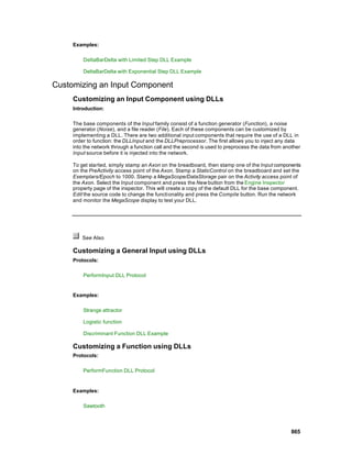

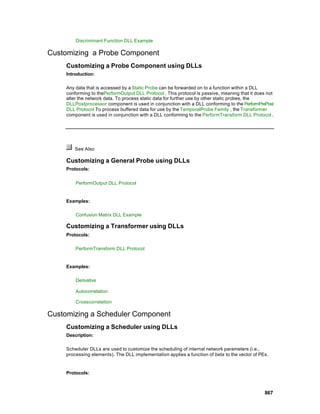
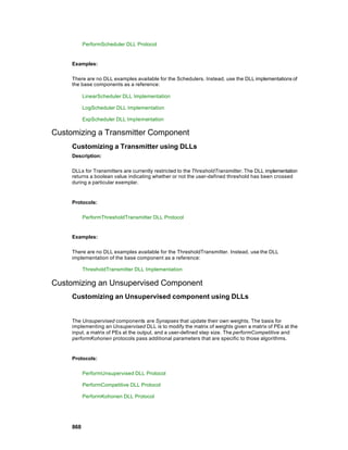

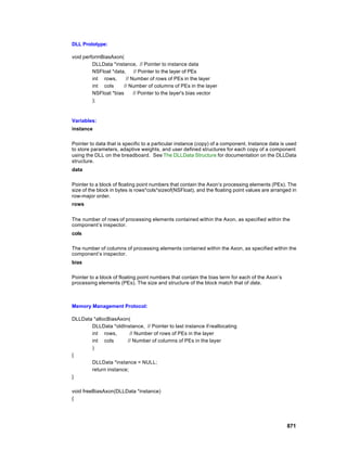

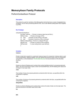
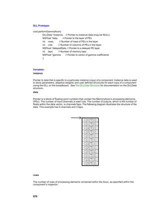


![A TDNNAxon with 1 channel and three taps is fed 6 samples of data. The first row of the table is
tap[0], which is the Axon’s input. Each column of the table shows that state of the 3 taps at a given
instant in time. Compare the two tables and note how the tap delay τ determines the memory
depth.
It is worth pointing out how the delayedData vector fits into this example. If τ is set to 1, then
delayedData would point to a block containing the values found in the time=4 column of the first
table. Likewise, If τ is set to 2, then delayedData would point to a block containing the values found
in the time=3 column of the second table.
See Also
FuzzyAxon Family Protocols
PerformFuzzyAxon Protocol
Description:
This protocol is used for members of the FuzzyAxon family that have all of the parameters
contained within the PerformAxon DLL Protocol protocol, with the addition of four parameters.
DLL Prototype:
void performFuzzyAxon(
DLLData*instance, // Pointer to instance data (may be NULL)
NSFloat*data, // Pointer to the layer of processing elements (PEs)
int rows, // Number of rows of PEs in the layer
int cols, // Number of columns of PEs in the layer
NSFloat*param, // Pointer to the layer of parameters for the MFs
int paramIndex, // Index into the param array
int PEIndex, // Index into the processing elements of the
880](https://image.slidesharecdn.com/neurosolutionshelp-090922003656-phpapp01/85/NeuroDimension-Neuro-Solutions-HELP-880-320.jpg)

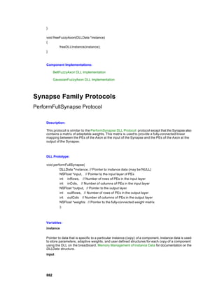


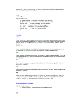
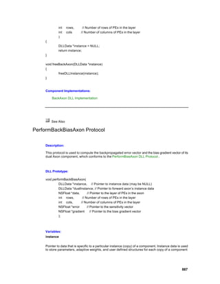


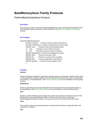
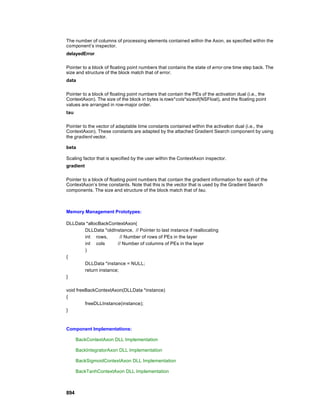
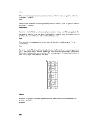

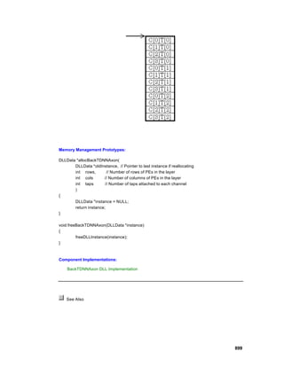

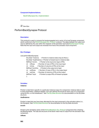


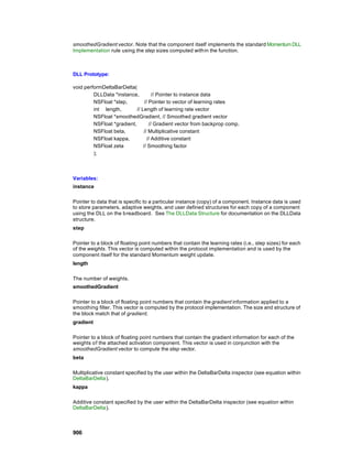
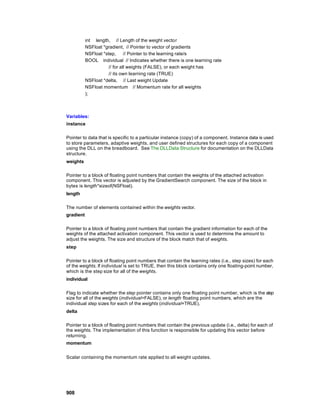


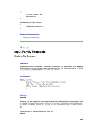

![cols
The number of columns of processing elements contained within the attached component, as
specified within the component’s inspector.
Memory Management Protocol:
DLLData *allocInput(
DLLData *oldInstance // Pointer to the last instance if reallocating
int rows, // Number of rows of data
int cols // Number of cols of data
)
{
DLLData *instance = allocDLLInstance(oldInstance);
return instance;
}
void freeInput(DLLData *instance)
{
freeDLLInstance(instance);
}
Component Implementations:
DLLInput DLL Implementation
See Also
PerformPrePost Protocol
Description:
This protocol is used for both preprocessing of network input as well as postprocessing of n etwork
output. The implementation of the performPrePost function reads the data from input and writes the
processed data to output. The function returns a TRUE if the output is to be passed on to the next
component, or FALSE if more data needs to be processed (more calls to performPrePost).
It is important to understand the distinction between the preprocessor and postprocessor modes.
The preprocessor gets its input from an Input component stacked above, and its output is the
vector of processing elements o f the component stacked below. The preprocessed output is
normally accumulated to the existing activity (e.g., data[i] = data[i] + preprocessedData[i]), in order
allow other components to inject data into the same component. The postprocessor’s input is the
vector of PEs of the component stacked below and its output is a locally-stored vector, which is
used by a Probe attached above. Note that this vector is not automatically zeroed, so that it can be
used to store the postprocessed data from the previous call to performPrePost.
918](https://image.slidesharecdn.com/neurosolutionshelp-090922003656-phpapp01/85/NeuroDimension-Neuro-Solutions-HELP-918-320.jpg)
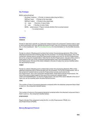


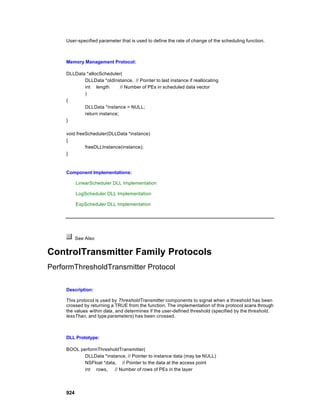


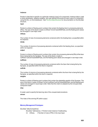

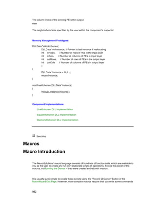
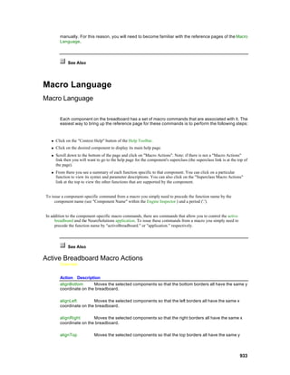
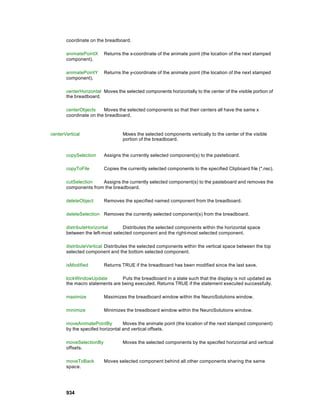
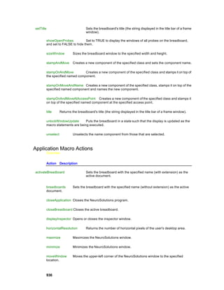
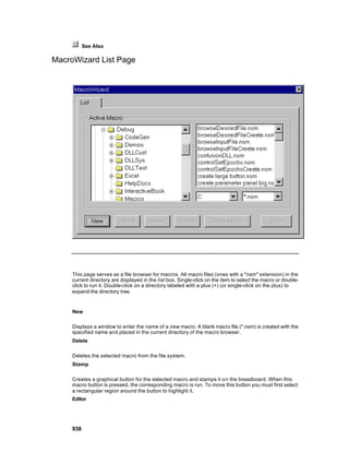


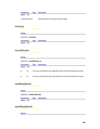


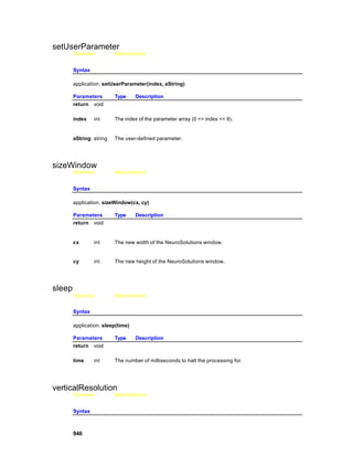
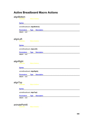
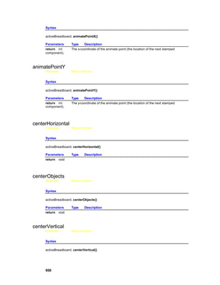
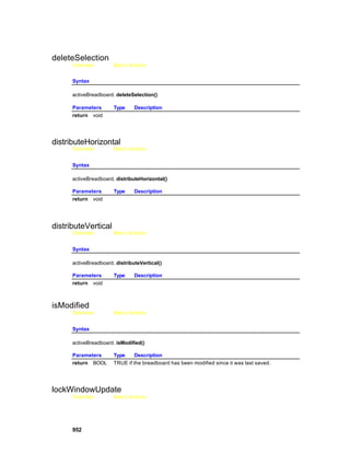
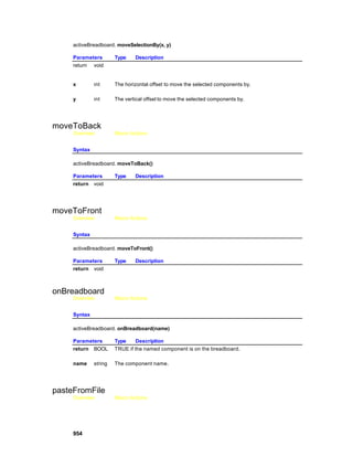


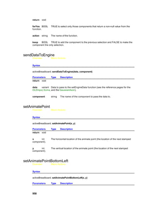
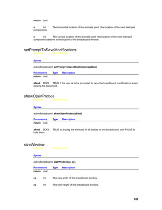
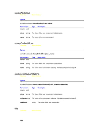
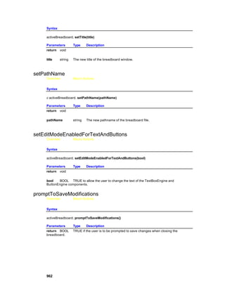


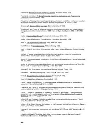

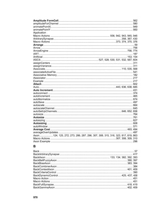

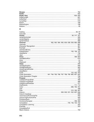
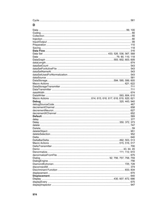
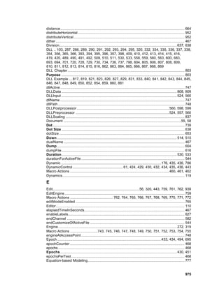
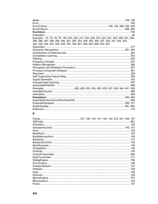

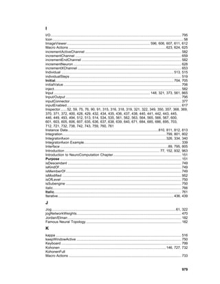
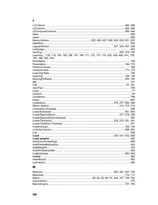

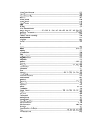
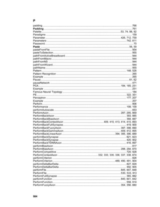
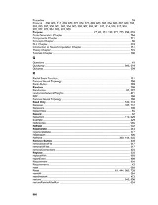


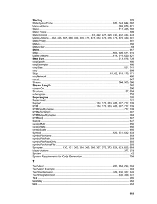
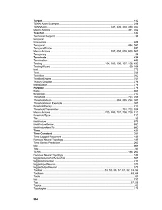

This document provides an overview of the NeuroSolutions software. It includes sections on product information, getting started, terms to know, menus and toolbars, component palettes, command toolbars, views, help, user options, examples, simulations, and concepts. The document introduces the key features and functionality of the software.