NEETRAC (Chapter 10: Monitored Withstand Techniques)

Copyright © 2016, Georgia Tech Research Corporation
Cable Diagnostic Focused Initiative (CDFI)
Phase II, Released February 2016
10-1
CHAPTER 10
Monitored Withstand Techniques
Jean Carlos Hernandez-Mejia
This chapter represents the state of the art at the time of release.
Readers are encouraged to consult the link below for the version of this
chapter with the most recent release date:
http://www.neetrac.gatech.edu/cdfi-publications.html
Users are strongly encouraged to consult the link below for the most recent
release of Chapter 4:
Chapter 4: How to Start

10-2
DISCLAIMER OF WARRANTIES AND LIMITATION OF LIABILITIES
This document was prepared by Board of Regents of the University System of Georgia by and on
behalf of the Georgia Institute of Technology NEETRAC (NEETRAC) as an account of work
supported by the US Department of Energy and Industrial Sponsors through agreements with the
Georgia Tech Research Institute (GTRC).
Neither NEETRAC, GTRC, any member of NEETRAC or any cosponsor nor any person acting on
behalf of any of them:
a) Makes any warranty or representation whatsoever, express or implied,
i. With respect to the use of any information, apparatus, method, process, or similar
item disclosed in this document, including merchantability and fitness for a
particular purpose, or
ii. That such use does not infringe on or interfere with privately owned rights, including
any party’s intellectual property, or
iii. That this document is suitable to any particular user’s circumstance; or
b) Assumes responsibility for any damages or other liability whatsoever (including any
consequential damages, even if NEETRAC or any NEETRAC representative has been
advised of the possibility of such damages) resulting from your selection or use of this
document or any information, apparatus, method, process or similar item disclosed in this
document.
DOE Disclaimer: This report was prepared as an account of work sponsored by an agency of the
United States Government. Neither the United States Government nor any agency thereof, nor any
of their employees, makes any warranty, express or implied, or assumes any legal liability or
responsibility for the accuracy, completeness, or usefulness of any information, apparatus, product,
or process disclosed, or represents that its use would not infringe privately owned rights. Reference
herein to any specific commercial product, process, or service by trade name, trademark,
manufacturer, or otherwise does not necessarily constitute or imply its endorsement,
recommendation, or favoring by the United States Government or any agency thereof. The views
and opinions of authors expressed herein do not necessarily state or reflect those of the United
States Government or any agency thereof.
NOTICE
Copyright of this report and title to the evaluation data contained herein shall reside with GTRC.
Reference herein to any specific commercial product, process or service by its trade name,
trademark, manufacturer or otherwise does not constitute or imply its endorsement,
recommendation or favoring by NEETRAC.
The information contained herein represents a reasonable research effort and is, to our knowledge,
accurate and reliable at the date of publication.
It is the user's responsibility to conduct the necessary assessments in order to satisfy themselves as
to the suitability of the products or recommendations for the user's particular purpose.

10-3
TABLE OF CONTENTS
10.0 Monitored Withstand Techniques................................................................................................ 6
10.1 Test Scope................................................................................................................................. 6
10.2 How it Works............................................................................................................................ 7
10.3 How it is Applied...................................................................................................................... 8
10.4 Success Criteria ...................................................................................................................... 12
10.5 Estimated Accuracy................................................................................................................ 13
10.6 CDFI Perspective ................................................................................................................... 13
10.6.1 Definition of a Withstand Test......................................................................................... 13
10.6.2 General Monitored Withstand Framework ...................................................................... 14
10.6.3 Evolution of VLF Tan δ Monitored Withstand Criteria................................................... 16
10.6.4 Monitored Withstand Using VLF Tan δ .......................................................................... 18
10.6.4.1 Decision 1 - “Ramp-up” Phase Evaluation – Continue to “Hold” Phase? ................ 20
10.6.4.2 Decision 2 – “Hold” Phase Evaluation – Amend Test Time? ................................... 25
10.6.4.3 Decision 3 – “Hold” Phase Evaluation – Final Assessment? .................................... 29
10.6.4.4 Case Studies............................................................................................................... 34
10.6.4.5 Comparison with Simple VLF Withstand.................................................................. 37
10.6.5 Monitored Withstand Using Partial Discharge ................................................................ 45
10.6.6 Monitored Withstand with Damped ac (DAC) Voltage Sources..................................... 46
10.6.7 Monitored Withstand Using DC Leakage Current........................................................... 46
10.7 Outstanding Issues.................................................................................................................. 46
10.7.1 Monitored Withstand Framework – PD and Leakage Current ........................................ 46
10.7.2 Criteria Based on Local and Global Data......................................................................... 47
10.8 References .............................................................................................................................. 48
10.9 Relevant Standards ................................................................................................................. 50
10.10 Appendix .............................................................................................................................. 51
10.10.1 Details of Feature Elimination Using Cluster Variable Analysis .................................. 51
10.10.2 Single Diagnostic Indicator Based on Principal Component Analysis (PCA)............... 53
10.10.3 PE-Based Insulation Final Assessment.......................................................................... 55
10.10.4 Filled Insulation Final Assessment ................................................................................ 62
10.10.5 PILC Insulation Final Assessment................................................................................. 66
LIST OF FIGURES
Figure 1: Schematic Representation of a Monitored Withstand Test.................................................. 7
Figure 2: Schematic of a Monitored Withstand Test with Optional Diagnostic Measurement
(Monitor).............................................................................................................................................. 8
Figure 3: Possible Characteristic Shapes of Monitored Responses................................................... 12
Figure 4: Monitored Withstand Test Framework .............................................................................. 14
Figure 5: Decision Making and Condition Assessment in the Context of a Monitored Withstand
Test Framework ................................................................................................................................. 16
Figure 6: Monitored Withstand Test Framework using VLF Tan δ Measurements.......................... 18
Figure 7: Description of the VLF Tan δ Monitored Withstand Database ......................................... 20

10-4
Figure 8: Examples of Measured Tan δ data and Diagnostic features from a PE Cable System during
the “Ramp-up” Phase......................................................................................................................... 21
Figure 9: Outcomes for Decision 1 – Continue to the “Hold” Phase?............................................... 25
Figure 10: Determining Critical Levels for Diagnostic Features for Test Time Amendment from
Research Data (PE-based Insulations)............................................................................................... 27
Figure 11: Outcomes for Decision 2 Using CDFI Research Data – Amend Test Time?.................. 29
Figure 12: Example of Real Measured Tan δ data and Diagnostic features from a PE Cable System
during the “Hold” Phase .................................................................................................................... 31
Figure 13: Comparison of Empirical Cumulative Distributions of the PCA Distance used for
Evaluation of the “Hold” Phase by Insulation Type.......................................................................... 33
Figure 14: Case Study 1: Field VLF Tan δ Monitored Withstand Data for a Service Aged XLPE
Cable System Ultimately Assessed as “No Action”.......................................................................... 34
Figure 15: Case Study 2: Field VLF Tan δ Monitored Withstand Data for a Service Aged XLPE
Cable System Ultimately Assessed as “Further Study”..................................................................... 36
Figure 16: Simple VLF Withstand Framework on the Basis of Number of Tested Cable Systems and
Test Time for PE-based Insulations................................................................................................... 38
Figure 17: Monitored VLF Withstand Framework on the Basis of Number of Tested Cable Systems
and Test Time for PE-based Insulations............................................................................................ 39
Figure 18: Comparison between Simple VLF (Red) and VLF Tan δ Monitored (Blue) Withstand
Frameworks on the Basis of Number of Tested Cable Systems and Test Time for PE-based
Insulations.......................................................................................................................................... 40
Figure 19: Graphical Interpretation of Principal Component Analysis (PCA).................................. 54
Figure 20: Calculation of the Single Diagnostic Indicator from PCA............................................... 54
Figure 21: Cluster Variable Analysis Results for PE-based Insulations (Based on data as described
in Table 4).......................................................................................................................................... 56
Figure 22: STD vs. SPD 0-tfinal (left) and PC1 vs. PC2 (right) – PE-based Insulations .................... 57
Figure 23: Empirical Cumulative Distribution of the PCA Distance used for Evaluation of the
“Hold” Phase for PE-based Cable Systems .......................................................................................59
“Hold” Phase for PE-based Cable Systems with Condition Assessment Categories ........................ 59
Figure 25: Empirical Cumulative Distribution of the PCA Distance from CDFI Research Used for
Evaluating the “Hold” Phase for PE-based Cable Systems with Relevant Case Studies from Table
19........................................................................................................................................................ 61
Figure 26: Cluster Variable Analysis Results for “Hold” Phase Features for Filled Insulations
(Based on data as described in Table 4)............................................................................................. 62
“Hold” Phase for Filled Cable Systems............................................................................................. 63
“Hold” Phase for Filled Cable Systems with Relevant Case Studies Presented in Table 21 ............ 65
Figure 29: Cluster Variable Analysis Results for the Diagnostic Features Selected to Characterize
the “Hold” Phase for Paper Insulations (Based on data as described in Table 4) ............................. 66
“Hold” Phase for Paper Cable Systems ............................................................................................. 67
“Hold” Phase for Paper Cable Systems with Relevant Case Studies Presented in Table 23............. 69

10-5
LIST OF TABLES
Table 1: Advantages and Disadvantages of Monitored Withstand for All Possible Different Voltage
Sources and Monitored Properties..................................................................................................... 10
Table 2: Overall Advantages and Disadvantages of Monitored Withstand Techniques ................... 11
Table 3: Evolution of VLF Tan δ Monitored Withstand Criteria for MV Cable Systems ................ 17
Table 4: Description of the VLF Tan δ Monitored Withstand Database........................................... 19
Table 5: CDFI Research Criteria for Evaluation of the “Ramp-up” Phase for PE-based Insulations22
Table 6: CDFI Research Criteria for Evaluation of the “Ramp-up” Phase of Filled Insulations...... 23
Table 7: CDFI Research Criteria for Evaluation of the “Ramp-up” Phase of Paper Insulations ...... 24
Table 8: CDFI Research Criteria for Time Amendment of the “Hold” Phase of PE-based Insulations
............................................................................................................................................................ 27
Table 9: CDFI Research Criteria for Time Amendment of the “Hold” Phase of Filled Insulations. 28
Table 10: CDFI Research Criteria for Time Amendment of the “Hold” Phase for Paper Insulations
............................................................................................................................................................ 28
Table 11: Comparison of PCA Results by Insulation Type............................................................... 32
Table 12: Case Study 1 - Field VLF Tan δ Monitored Withstand Data and Decision Making
Framework for a Service Aged XLPE Cable System Assessed as “No Action”............................... 35
Framework for a Service Aged XLPE Cable System Assessed as “Further Study” ......................... 37
Table 14: Comparison between VLF Tan δ Monitored and Simple Withstand Frameworks for PE-
based Insulations................................................................................................................................ 42
Table 15: Comparison between VLF Tan δ Monitored and Simple Withstand Frameworks for Filled
Insulations.......................................................................................................................................... 43
Table 16: Comparison between VLF Tan δ Monitored and Simple Withstand Frameworks for Paper
Insulations.......................................................................................................................................... 44
Table 17: Comparison between VLF Tan δ Monitored Frameworks Including all Insulation Types45
Table 18: PCA Variances and Component Composition for PE-based Insulations.......................... 58
Table 19: Cases Studies for “Hold” Phase Evaluation for PE-based Insulations.............................. 60
Table 20: PCA Variances and Component Composition for Filled Insulations................................ 63
Table 21: Cases Studies for “Hold” Phase Evaluation for Filled Insulations.................................... 64
Table 22: PCA Variances and Component Composition for Paper Insulations................................ 67
Table 23: Cases Studies for “Hold” Phase Evaluation for Paper Insulations.................................... 68

10-6
10.0 MONITORED WITHSTAND TECHNIQUES
10.1 Test Scope
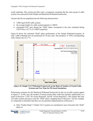
Simple Withstand tests are proof tests that apply voltage above the normal operating voltage to
stress the insulation of a cable system in a prescribed manner for a set period of time (time-voltage
recipe) [1-15]. This is similar to tests applied to new accessories or cables in the factory where a
withstand voltage is applied to provide the purchaser with assurance that the component can
withstand a defined voltage. An alternative and more sophisticated implementation of the simple
withstand approach requires that, in addition to surviving an applied voltage stress, a system
property is also measured during the test. The property measured should be selected to correlate
with the condition of the system. This implementation of a withstand test, called Monitored
Withstand test, is discussed in this chapter and is more sophisticated than a Simple Withstand.
In traditional Simple Withstand tests (VLF, dc, or resonant ac), a significant drawback is the
absence of a straightforward way to estimate the “Pass” margin. Once a test (e.g. 30 min at 2 U0,
where U0 is the nominal system operation voltage) is completed, it is impossible to differentiate
among those cable systems that survived the test without failure. As a result, this test cannot
distinguish cable system segments that pass the test, but would survive only minutes or days after
the test from those that could last months or years after the test.
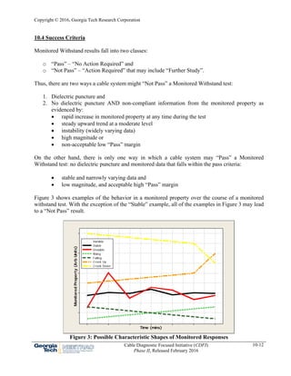
Thus, it is useful to employ the concept of a Monitored Withstand test whereby a dielectric property
or discharge characteristic is monitored to provide additional data. There are four ways these data
are useful in making decisions during the test:
1. Provides an estimate of the “Pass” margin for cable systems that have not failed during the
hold phase of the Monitored Withstand test.
2. Enables a utility to stop a test after a short time if the monitored property indicates the cable
system is near imminent failure on test thereby allowing the required remediation work to
take place at a convenient (lowest cost) time.
3. Enables a utility to stop a test early (shorten the duration of the test) if the monitored
property provides definitive evidence of good performance, thereby increasing the number
of tests that could be completed and improving the overall efficiency of field testing.
4. Enables a utility to extend a test if the monitored property provides indications that the
“Pass” margin was questionable, thereby focusing test resources on sections that present the
most concern.
In fact, the design of the decision making process can be accomplished by advanced statistical
analysis of the data accumulated during CDFI Phases I and II. This allows for the creation of
defined and well-organized monitored withstand testing procedures that can be deployed in real
time in the field.

10-7
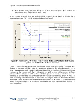
10.2 How it Works
In a Simple Withstand test, the applied voltage is quickly raised to a prescribed level, usually 1.5 to
2.5 U0 for a set amount of time. The purpose is to cause weak points in the cable system to fail
during the elevated voltage application when the system is not supplying customers. This avoids a
service failure and the associated reliability penalties as well as potential upstream fault current
damage. Testing is usually scheduled by the utility so that it occurs at a time when the impact of a
failure (if it occurs) is low and repairs can be made quickly and cost effectively.
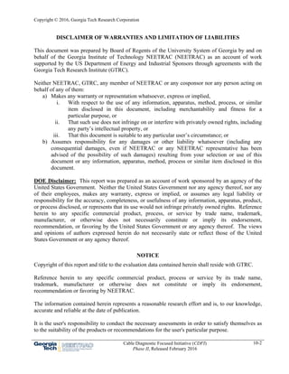
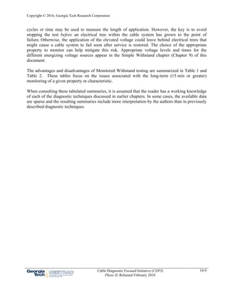
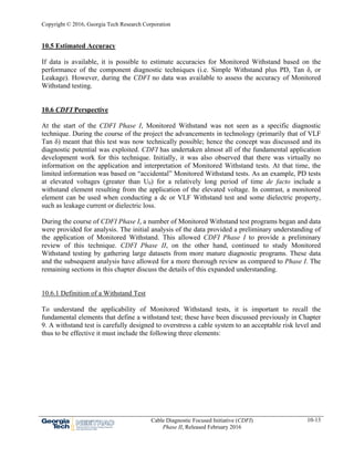
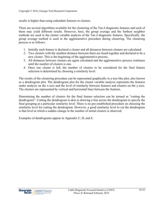
In contrast, when performing a Monitored Withstand test, a dielectric or discharge property is
monitored during the withstand period or “Hold” phase of the test (see Figure 1). The data and its
interpretation should be accessible in real time during the test so that the decisions outlined above
can be made.
Figure 1: Schematic Representation of a Monitored Withstand Test
The dielectric or discharge monitored property are similar to those described in earlier chapters.
However, their implementation and interpretation differs due to the requirement of a fixed voltage
and a relatively long period of voltage application for the “Hold” phase of the test. Within these
constraints, Leakage Current, Partial Discharge (magnitude and repetition rate) and Tan δ (stability,
magnitude, and rate of change over time (speed)) [2] might readily be used as monitors.

10-8
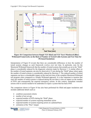
10.3 How it is Applied
This technique is conducted offline with the system disconnected from the network. The applied
voltage may be dc (not recommended for most applications), VLF (sinusoidal or cosine-
rectangular), or 10 - 300 Hz ac using a resonant power supply. Typical testing voltages range from
1.5 - 4.0 U0 [1-15] though the precise levels depend upon the voltage source, (VLF levels tend to be
lower than dc). If a failure occurs during the test according to either of the two criteria (dielectric
puncture or unacceptable monitored property) then the cable system is remediated or repaired and
the circuit is retested for the full test time. The inadvisability of using damped ac voltages for
withstand purposes is discussed later in Section 10.6.2.
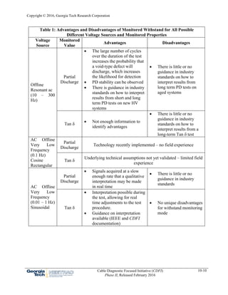
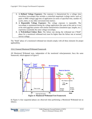
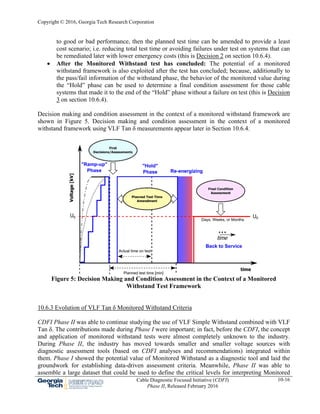
In Figure 1, the schematic represents a monitored withstand test. The critical part of the test is the
measurement and interpretation during the “Hold” phase. However, it is clear that the simple
scheme in Figure 1 could be modified to allow an evaluation before the start of the withstand test as
shown schematically in Figure 2. This approach is valuable in that it enables the field engineers to
assess the condition of the cable system before embarking on the monitored withstand test.
Figure 2: Schematic of a Monitored Withstand Test with Optional Diagnostic Measurement
(Monitor)
Like other diagnostic techniques, Simple and Monitored Withstand tests require the application of
voltages in excess of the service voltage for extended time periods (up to 60 min). However, unlike
many other diagnostic test techniques, a failure on test (FOT) is an acceptable (almost desirable)
outcome. The expectation is that the proof stress will cause the weak components to fail without
significantly shortening the life of the vast majority of strong components.
The risk of excessive FOTs through unintended degradation of the stronger elements is reduced by
using voltages closer to the service level and limiting the duration of the test. Either the number of

10-9
cycles or time may be used to measure the length of application. However, the key is to avoid
stopping the test before an electrical tree within the cable system has grown to the point of
failure. Otherwise, the application of the elevated voltage could leave behind electrical trees that
might cause a cable system to fail soon after service is restored. The choice of the appropriate
property to monitor can help mitigate this risk. Appropriate voltage levels and times for the
different energizing voltage sources appear in the Simple Withstand chapter (Chapter 9) of this
document.
The advantages and disadvantages of Monitored Withstand testing are summarized in Table 1 and
Table 2. These tables focus on the issues associated with the long-term (15 min or greater)
monitoring of a given property or characteristic.
When consulting these tabulated summaries, it is assumed that the reader has a working knowledge
of each of the diagnostic techniques discussed in earlier chapters. In some cases, the available data
are sparse and the resulting summaries include more interpretation by the authors than in previously
described diagnostic techniques.

10-10
Table 1: Advantages and Disadvantages of Monitored Withstand for All Possible
Different Voltage Sources and Monitored Properties
Voltage
Source
Monitored
Value
Advantages Disadvantages
Offline
Resonant ac
(10 – 300
Hz)
Partial
Discharge
 The large number of cycles
over the duration of the test
increases the probability that
a void-type defect will
discharge, which increases
the likelihood for detection
 PD stability can be observed
 There is guidance in industry
standards on how to interpret
results from short and long
term PD tests on new HV
systems
 There is little or no
guidance in industry
standards on how to
interpret results from
long term PD tests on
aged systems
Tan δ
 Not enough information to
identify advantages
standards on how to
interpret results from a
long-term Tan δ test
AC Offline
Very Low
Frequency
(0.1 Hz)
Cosine
Rectangular
Partial
Discharge
Technology recently implemented – no field experience
Tan δ
Underlying technical assumptions not yet validated – limited field
experience
AC Offline
Very Low
Frequency
(0.01 – 1 Hz)
Sinusoidal
Partial
Discharge
 Signals acquired at a slow
enough rate that a qualitative
interpretation may be made
in real time
standards
Tan δ
 Interpretation possible during
the test, allowing for real
time adjustments to the test
procedure.
 Guidance on interpretation
available (IEEE and CDFI
documentation)
 No unique disadvantages
for withstand monitoring
mode

10-11
Table 2: Overall Advantages and Disadvantages of Monitored Withstand Techniques
Advantages
 Provides additional information over the simple “Pass” or “Not Pass” obtained
from a Simple Withstand test.
 Allows for the development of trending information during a single test.
 Diagnostic stability can be established during the test.
 Provides real time feedback so that the test may be adapted (test time
increased or decreased) to fit utility objectives.
 Cable system population under test can be selected to undergo different test
phases (population amendment and risk management).
 Many tests can be curtailed after 15 min and so Monitored Withstand requires
considerably less total test time when compared to a Simple Withstand
approach (40% to 60 % efficiency improvement).
 Allows for the integration of outcomes from Simple Withstand test with those
from other diagnostic techniques (two diagnostics and thus higher information
content).
 Less number of FOTs and thus less number of thumper tests for failure
location, which results in reduced work and emergency cost.
Open Issues
 Can potentially provide means for estimating a “Pass” margin for cable
systems that survive the “Hold” phase of the test.
 Selection of the best monitored property (i.e. PD, Tan δ, or Leakage).
 Implementation where only level-based assessments (Good/Bad) are available
is unclear and may not be useful.
 Voltage exposure (impact of voltage/time on cable system) caused by DAC
voltages has not been established.
Disadvantages
 Adds complexity (interpretation, set up, and data recording) to Simple
Withstand test.
 Highly skilled and fast decision-making personnel required.
A critical issue for Monitored Withstand testing, like Simple Withstand, is the application time at
the chosen voltage for the test. If the test time is too short then cable systems with localized defects
that could cause service failures may be returned to service before the defect has the chance to fail
during the test. Equally, a shortened test may not provide enough opportunity for the monitored
feature to provide useful information. As an example, an upward trend in a monitored property with
time usually indicates a problem. However, if the test time, and thus, the time to observe the trend is
too short then it is more difficult to unambiguously identify the trend and make a diagnosis.
The work described in the Simple Withstand chapter (Chapter 9) suggests that 30 minutes should be
the usual target test time. This is in accordance with the test time suggested by IEEE Std. 400.2 –
2013. This time may be increased to 60 minutes if the monitored data indicate instability or an
upward trend that indicates unsatisfactory performance. The test time may also be reduced to 15
minutes if experience shows that the monitored data definitively confirm good cable system
performance. Criteria for test time amendment appears later in this chapter.

10-12
10.4 Success Criteria
Monitored Withstand results fall into two classes:
o “Pass” – “No Action Required” and
o “Not Pass” – “Action Required” that may include “Further Study”.
Thus, there are two ways a cable system might “Not Pass” a Monitored Withstand test:
1. Dielectric puncture and
2. No dielectric puncture AND non-compliant information from the monitored property as
evidenced by:
 rapid increase in monitored property at any time during the test
 steady upward trend at a moderate level
 instability (widely varying data)
 high magnitude or
 non-acceptable low “Pass” margin
On the other hand, there is only one way in which a cable system may “Pass” a Monitored
Withstand test: no dielectric puncture and monitored data that falls within the pass criteria:
 stable and narrowly varying data and
 low magnitude, and acceptable high “Pass” margin
Figure 3 shows examples of the behavior in a monitored property over the course of a monitored
withstand test. With the exception of the “Stable” example, all of the examples in Figure 3 may lead
to a “Not Pass” result.
Time (mins)
MonitoredProperty(ArbUnits)
Stable
Unstable
Rising
Falling
Crook Up
Crook Down
Variable
Figure 3: Possible Characteristic Shapes of Monitored Responses

10-13
10.5 Estimated Accuracy
If data is available, it is possible to estimate accuracies for Monitored Withstand based on the
performance of the component diagnostic techniques (i.e. Simple Withstand plus PD, Tan δ, or
Leakage). However, during the CDFI no data was available to assess the accuracy of Monitored
Withstand testing.
10.6 CDFI Perspective
At the start of the CDFI Phase I, Monitored Withstand was not seen as a specific diagnostic
technique. During the course of the project the advancements in technology (primarily that of VLF
Tan δ) meant that this test was now technically possible; hence the concept was discussed and its
diagnostic potential was exploited. CDFI has undertaken almost all of the fundamental application
development work for this technique. Initially, it was also observed that there was virtually no
information on the application and interpretation of Monitored Withstand tests. At that time, the
limited information was based on “accidental” Monitored Withstand tests. As an example, PD tests
at elevated voltages (greater than U0) for a relatively long period of time de facto include a
withstand element resulting from the application of the elevated voltage. In contrast, a monitored
element can be used when conducting a dc or VLF Withstand test and some dielectric property,
such as leakage current or dielectric loss.
During the course of CDFI Phase I, a number of Monitored Withstand test programs began and data
were provided for analysis. The initial analysis of the data provided a preliminary understanding of
the application of Monitored Withstand. This allowed CDFI Phase I to provide a preliminary
review of this technique. CDFI Phase II, on the other hand, continued to study Monitored
Withstand testing by gathering large datasets from more mature diagnostic programs. These data
and the subsequent analysis have allowed for a more thorough review as compared to Phase I. The
remaining sections in this chapter discuss the details of this expanded understanding.
10.6.1 Definition of a Withstand Test
To understand the applicability of Monitored Withstand tests, it is important to recall the
fundamental elements that define a withstand test; these have been discussed previously in Chapter
9. A withstand test is carefully designed to overstress a cable system to an acceptable risk level and
thus to be effective it must include the following three elements:

10-14
1. A Defined Voltage Exposure: The exposure is characterized by a voltage time
waveform (waveshape) that includes a controlled magnitude (voltage metric such as
peak or RMS voltage) and time of application (in terms of specified time, number of
cycles, shots, or any other convenient time metric).
2. A Repeatable Voltage Exposure: The voltage exposure is repeatable. The
waveshape is maintained during the voltage application (the same at the end as it was
at the start) and that systems with similar characteristics (insulation type, lengths, etc.)
experience essentially the same voltage waveshape.
3. A Well-defined Failure Rate: The failure rate during the withstand test (“Hold”
phase for a monitored withstand test) must be higher than the failure rate at normal
service voltage.
The “Hold” phase of a monitored withstand test should comply with all three elements for proper
applicability.
10.6.2 General Monitored Withstand Framework
All Monitored Withstand tests, independent of the monitored value/parameter, have the same
framework, which appears in Figure 4.
Figure 4: Monitored Withstand Test Framework
In Figure 4, four sequential phases are observed when performing a Monitored Withstand test as
follows:

10-15
 “Ramp-up” phase: This is the initial stage of any Monitored Withstand test (i.e. after a
cable system has been taken off-line and properly grounded for testing). This involves
raising the test voltage from zero to the required withstand level. The monitored property
can be recorded during this stage and may be used to further develop the condition
assessment.
 “Hold” phase: This stage involves the actual withstand evaluation, the test voltage is held
constant and the monitored property is recorded for the duration of the test.
 Re-energization phase: This stage involves all the actions and time required to put a cable
system back in service once it has successfully completed the monitored withstand test
without a FOT.
 Back to Service phase: This stage represents operation of the cable system after testing.
There are two possibilities for the timing of a failure during a Monitored Withstand test: (1) during
the test itself (“Ramp-up” or “Hold” phases, FOT1 or FOT2, respectively, in Figure 4) or (2) after
test (Back to Service Phase, FIS1 or FIS2 in Figure 4). If the failure occurs on test, then the
Monitored Withstand test has successfully failed a weak location in the cable system and thus
accomplished its goal. Under this scenario, a Monitored Withstand test does not differ much from a
Simple Withstand test because both produce a failure irrespective of the monitored property
behavior.
The most useful aspect of the monitoring portion is that it may be used to estimate the “Pass”
margin (i.e. the system condition when no dielectric puncture occurred during the test). The concept
of “Pass” margin is only possible under the Monitored Withstand framework. At this stage, the
monitored property can be used to establish the degree of the “Pass” margin as either “Poor” or
“Better”. As shown in Figure 4, a “Poor” pass margin is defined as one in which the segment has a
high likelihood of failing in service minutes to days after the test concludes, while a “Better” pass
margin segment is likely to survive in service without failure months to years after the test. As with
all other diagnostic techniques, the key is defining the “likely” part of the previous statement.
The additional information afforded by Monitored Withstand does not come for free because there
is added complexity imposed by the diagnostics and decisions of the Monitored Withstand.
However, it allows for decision making during test deployment and data analysis for condition
assessment during and after the test has concluded. Therefore, in general, decisions and condition
assessments can be undertaken at three points as follows:
 At the end of the “Ramp-up” phase and before the beginning of the “Hold” phase: The
first decisions and condition assessments can be undertaken by evaluating the monitored
value/parameters and deciding which systems go to the “Hold” Phase. The reasoning here is
simple and is based on the potential that the monitored value/parameter has on detecting
extremes on the good and bad conditions. Thus good or bad systems do not need further
evaluation because their conditions have already been established and from a condition
assessment perspective continuing to the “Hold” phase is not an optimal use of resources
(this is Decision 1 on section 10.6.4).
 During the “Hold” phase: Decisions can only be undertaken here regarding the duration of
the withstand phase. Decisions are then based on ‘real time’ observation and analysis of the
monitored value. If the monitored value shows certain characteristics that can be correlated

10-16
to good or bad performance, then the planned test time can be amended to provide a least
cost scenario; i.e. reducing total test time or avoiding failures under test on systems that can
be remediated later with lower emergency costs (this is Decision 2 on section 10.6.4).
 After the Monitored Withstand test has concluded: The potential of a monitored
withstand framework is also exploited after the test has concluded; because, additionally to
the pass/fail information of the withstand phase, the behavior of the monitored value during
the “Hold” phase can be used to determine a final condition assessment for those cable
systems that made it to the end of the “Hold” phase without a failure on test (this is Decision
3 on section 10.6.4).
Decision making and condition assessment in the context of a monitored withstand framework are
shown in Figure 5. Decision making and condition assessment in the context of a monitored
withstand framework using VLF Tan δ measurements appear later in Section 10.6.4.
Figure 5: Decision Making and Condition Assessment in the Context of a Monitored
Withstand Test Framework
10.6.3 Evolution of VLF Tan δ Monitored Withstand Criteria
CDFI Phase II was able to continue studying the use of VLF Simple Withstand combined with VLF
Tan δ. The contributions made during Phase I were important; in fact, before the CDFI, the concept
and application of monitored withstand tests were almost completely unknown to the industry.
During Phase II, the industry has moved towards smaller and smaller voltage sources with
diagnostic assessment tools (based on CDFI analyses and recommendations) integrated within
them. Phase I showed the potential value of Monitored Withstand as a diagnostic tool and laid the
groundwork for establishing data-driven assessment criteria. Meanwhile, Phase II was able to
assemble a large dataset that could be used to define the critical levels for interpreting Monitored

10-17
Withstand data. To put this in perspective, the contributions of CDFI Phases I and II, Table 3 shows
the evolution of VLF Tan δ monitored withstand criteria.
Table 3: Evolution of VLF Tan δ Monitored Withstand Criteria for MV Cable Systems
Year
Assessment
Hierarchy
Criteria & Issues Comments (See 10.6.4)
< 2001 None None No framework established
2004 CDFI Phase I
2006
1. Trend
2. Stability
3. Level of
loss
Initial Discussion  Contribution of CDFI Phase I
project based on statistical analysis
of data from North American cables
 Initial quantitative criteria on
Decision 3 – Final Assessment?
Only for paper insulations
 Initial quantitative criteria on
Decision 2 – Amend of test time?
 First Tan δ Monitored Withstand
brochure
2007 Qualitative Experiments
2008 –
2010
 Criteria based on data
 Included in discussions of
IEEE Std. 400.2 – 2013
2011 CDFI Phase II
2011 –
2014
1. Trend
2. Stability
3. Level of
loss
 Criteria based on data.
 Included in update of
IEEE Std. 400.2 – 2013
 Increase the size of the Tan δ
monitored withstand database.
 Criteria on Decision 1 – Continue to
“Hold” phase?
 Criteria on Decision 2 – Amend of
test time?
 IEEE Std. 400.2TM
– 2013 release.
 Continuing update of Tan δ brochure
2015
1. Speeds
2. Stability
3. Level of
loss
 Criteria based on data
 Verification of Tan 
diagnostic features and
hierarchy
 VLF Tan δ monitored
withstand framework.
 Evaluation of the “Ramp-
up” Phase
 Amendment of test time.
 Evaluation of the “Hold”
phase & Final
Assessment
 PCA-based analysis tool
 Contribution of CDFI Phase II
Project based on statistical analysis
of data from North American cables
 Criteria on Decision 1 – Continue to
“Hold” phase?
 Criteria on Decision 2 – Amend of
test time?
 Criteria on Decision 3 – Final
Assessment?
 Established complete framework.
 Continuing update of Tan δ brochure

10-18
It is important to note the use of the term “Qualitative” in Table 3 is used to describe some of
criteria in 2007. This term is used because the understanding in CDFI Phase I at the time was
limited to which VLF Tan δ measurement values were “really good” and those that were “really
bad” but there was not a defined threshold to separate these two categories. Thresholds and criteria
were developed later once significant amounts of data were available.
10.6.4 Monitored Withstand Using VLF Tan δ
There are a number of monitored properties that could be utilized during a Monitored Withstand
test. They each entail their own difficulties. This section describes the implementation of Monitored
Withstand using VLF Tan δ as the monitored property. The basic framework appears in Figure 6.
Figure 6: Monitored Withstand Test Framework using VLF Tan δ Measurements
As Figure 6 illustrates, there are three sequential decisions to be made as part of the Monitored
Withstand test, namely:
 Decision 1 – Continue to “Hold” phase? It is based on the evaluation of the “Ramp-up”
phase that can be related to a conventional VLF Tan δ test as described in Chapter 6
(Dissipation Factor – Tan δ). Therefore, Decision 1 can be made by both using reference
tables or “Health Index” based on the PCA tool developed in the CDFI. Since Decision 1
has to be made on-site during the test, the use of reference tables is preferred over the PCA
tool because it is faster and easier to use. Criteria for Decision 1 based on reference tables
appear in Table 5 to Table 7 for all insulation types.
 Decision 2 – Amend test time? It is based on an initial evaluation of the “Hold” phase to
amend test time. Since Decision 2 has also to be made on site during the test, reference table

10-19
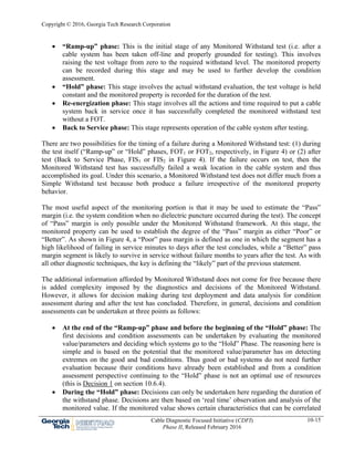
based criteria are also used. Criteria for Decision 2 based on reference tables appear in Table
8 to Table 10 for all insulation types.
 Decision 3 – Final assessment? If the monitored withstand test has concluded without a
FOT, Decision 3 is based on a final evaluation of the “Hold” phase. Since this decision can
be made after the test has concluded, it is made by estimating the “Pass” margin using a
single diagnostic indicator based on PCA. This complication is not as time sensitive and so
does not impact the decision making that must occur during the test.
Each of the above decisions is discussed in detail in Sections 10.6.4.1 through 10.6.4.3. It is
important to note that Decision 1 and Decision 2 are made in real time as part of the testing
procedure while Decision 3 can be made afterwards. Within each of these sections, criteria are
provided for aiding users in making the real time and post-test decisions. These criteria were
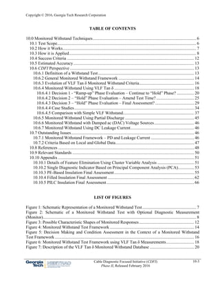
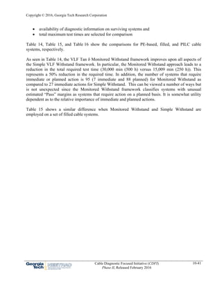
developed from an extensive VLF Tan δ Monitored Withstand database as summarized in Table 4.
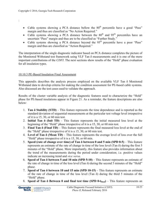
Table 4: Description of the VLF Tan δ Monitored Withstand Database
Insulation Type
Number of Tests Tested Length
Absolute
[#]
Proportion
[%]
Absolute
[mi]
Proportion
[%]
PE-based
(i.e. PE, HMWPE, XLPE, &
WTRXLPE)
618 44.6 366.7 39.4
Filled
(i.e. EPR & Vulkene)
237 17.1 110.3 11.9
Paper
(i.e. PILC)
513 37.0 409.2 44.0
Hybrid 17 1.2 43.9 4.7
Total 1,385 100.0 930.0 100.0
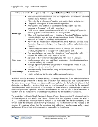
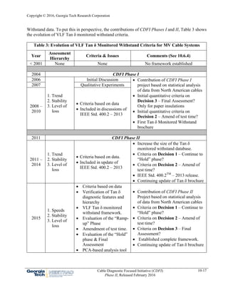
This database includes 1,385 tests on 930 miles of cable system made during 2007 - 2015. The tests
encompass a wide variety of cable systems including PILC, PE-based, filled, and hybrid systems.
Figure 7 shows the split in terms of both number of tests and length tested for each system type.

10-20
Filled
Hy brid
Paper
PE-based
Insulation
44.6%
37.0%
1.2%
17.1%
4.7%
11.9%
39.4%
44.0%
Number of Tests
Total of 1385 tests from 2007 to 2015
Total Tested Length
(A pprox. 5 million ft or 582 km)
Total Tested Length: 931 miles
Figure 7: Description of the VLF Tan δ Monitored Withstand Database
Unfortunately, there are too few data to develop criteria for all system types. However, criteria were
developed wherever possible as illustrated in the Decision 1 criteria discussed in the next section.
10.6.4.1 Decision 1 - “Ramp-up” Phase Evaluation – Continue to “Hold” Phase?
As seen in Figure 6, Decision 1 is based on the “Ramp-up” phase evaluation. During this phase, the
test voltage is increased from zero to the required test voltage level in steps of 0.5 U0 as the required
withstand voltage level is usually greater than 1.5 U0. The resulting “Ramp-up” phase consists of
three steps of 0.5 U0, U0, and 1.5 U0 with Tan δ measurements at each step. It is important to relate
the evaluation of the “Ramp-up” phase to a conventional VLF Tan δ test as defined in Chapter 6
Dissipation Factor (Tan δ).
Consequently, the evaluation of the “Ramp-up” phase uses the following Tan δ diagnostic features
listed in order of decreasing importance as follows:
 Tan δ Stability – This feature represents the time dependence and is normally reported as
the standard deviation (STD) of sequential measurements at U0.
 Differential Tan δ or Tip Up – This feature represents the voltage dependence and is
normally reported as the simple algebraic difference between the means of a number of
sequential measurements taken at two different voltages, in this case the voltage levels are
0.5 U0 and 1.5 U0.
 Tip Up of the Tip Up (TuTu) – This feature represents the nonlinear voltage dependence

10-21
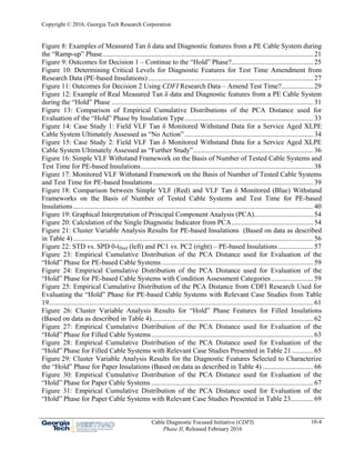
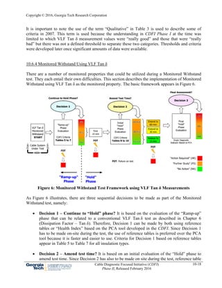
and it is reported as the algebraic difference between two Tip Ups: the Tip Up between 1.5
U0 and U0 and the Tip Up between U0 and 0.5 U0.
 Level of Tan δ – This feature represents the level of loss and is normally reported as the
mean of a number of sequential measurements (the median of these measurements may also
be used) at U0.
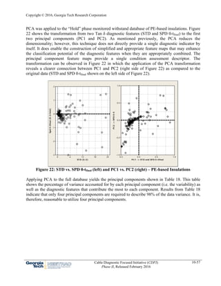
Figure 8 shows examples of measured Tan δ data during the “Ramp-up” phase and the
corresponding diagnostic features from a PE-based cable system. The diagnostic features for other
insulation types (filled and paper) are the same as the ones described in Figure 8.
43210
3.0
2.5
2.0
1.5
1.0
Time [min]
TD[E-3]
0.5
1.0
1.5
Voltage Uo
Measurement Sequence
Mean TD at 0.5 Uo
Mean TD at Uo
Mean TD at 1.5 Uo
Six measurements per voltage level
Mean TD at Uo
Feature 4 - Level of Loss:
Standard Deviation at Uo
Feature 1 - Time Dependence:
Tip Up between 0.5 Uo and 1.5 Uo
Feature 2 - Voltage Dependence:
Uo to 1.5 Uo
Tip Up
0.5 Uo to Uo
Tip Up
A
B
Tip Up of the Tip Up (TuTu) = A-B
TuTu between 0.5 Uo, Uo, and 1.5 Uo
Feature 3 - Nonlinear Voltage Dependence:
Figure 8: Examples of Measured Tan δ data and Diagnostic features from a PE Cable System
during the “Ramp-up” Phase
The criteria for evaluation of the “Ramp-up” phase are the same as those developed in Chapter 6 but
reappear in Table 5 to Table 7. In these tables, the typical Tan δ assessment classes of (“No Action
Required”, “Further Study”, and “Action Required”) have been replaced with No/Yes to correspond
to the Decision 1 question: Continue to “Hold” phase?

10-22
Table 5: CDFI Research Criteria for Evaluation of the “Ramp-up” Phase for PE-based
Insulations
(i.e. PE, HMWPE, XLPE, & WTRXLPE)
Decision 1 – Continue to “Hold” Phase?
“Ramp-up” Phase Evaluation
[E-3]
“No”* “Yes”** “No”***
Stability for TDU0
(standard deviation – STD)
<0.1 0.1 to 1.0 >1.0
and or
Tip Up
(TD1.5U0 – TD0.5U0 – TU)
<6.7 6.7 to 94.0 >94.0
and or
Tip Up Tip Up (TuTu)
{(TD1.5U0–TDU0) - (TDU0–TD0.5U0)} <2.0 2.0 to 50.0 >50.0
Mean Tan δ at U0 (TD)
and or
<6.0 6.0 to 70.0 >70.0
* “Green No” – Cable systems condition is assessed as in the best performing 80% and thus it is
unnecessary to continue to “Hold” phase because time and resources are saved.
** “Amber Yes” – Cable system condition cannot be determined during the “Ramp-up” phase
and thus systems are further taken to the “Hold” phase for a final condition assessment.
*** “Red No” – Cable system condition is assessed as in the poorest performing 5% and thus it is
unnecessary to continue to the “Hold” phase because the higher risk of FOT is likely to result
in inefficient testing and high emergency repair costs. Systems in this category can be acted on
in a planned manner by managing optimal time and costs.

10-23
Table 6: CDFI Research Criteria for Evaluation of the “Ramp-up” Phase of Filled Insulations
(i.e. EPR & Vulkene®
)
“Ramp-up” Phase
Evaluation
[E-3]
“No”* “Yes”** “No”***
Unidentified Filled Insulations
(i.e. EPR, Kerite, & Vulkene®
)*
Stability for TDU0
<0.1 0.1 to1.2 >1.2
and or
Tip Up
(TD1.5U0 – TD0.5U0 – TU)
<3.0 3.0 to 30.0 >30.0
and or
{(TD1.5U0–TDU0) - (TDU0–
TD0.5U0)}
<1.0 1.0 to 18.0 >18.0
and or
<25.0 25.0 to 150.0 >150.0
Mineral Filled Insulations (i.e. EPR)
Experience has shown that it is difficult to precisely identify the type of filled insulation in field-
installed cable. The issues include: incorrect /missing records, obscured markings on the jacket,
indistinct coloring, etc. In these cases, it is recommended to use the criteria for Unidentified Filled.
Stability for TDU0
<0.1 0.1 to 0.8 >0.8
and or
Tip Up
(TD1.5U0 – TD0.5U0 – TU)
<2.0 2.0 to 40.0 >40.0
and or
{(TD1.5U0–TDU0) - (TDU0–
TD0.5U0)}
<1.0 1.0 to 25.0 >25.0
and or
<16.0 16.0 to 75.0 >75.0
* “Green No” – Cable system condition is assessed as in the best performing 80% and thus it is
unnecessary to continue to “Hold” phase because time and resources are saved.
*** “Red No” – Cable system condition is assessed as in the poorest performing 5% and thus it is
unnecessary to continue to the “Hold” phase because the higher risk of FOT is likely to result
in inefficient testing and high emergency repair cost. Systems in this category can be acted on
a planned manner by managing optimal time and costs.

10-24
Table 7: CDFI Research Criteria for Evaluation of the “Ramp-up” Phase of Paper Insulations
(i.e. PILC)
“Ramp-up” Phase
Evaluation
[E-3]
“No”* “Yes”** “No”***
Stability for TDU0
<0.2 0.2 to 1.5 >1.5
and or
Tip Up
(TD1.5U0 – TD0.5U0 – TU)
-30.0
to
22.0
-30.0 to -60.0
or
22.0 to 220.0
<-60.0
or
>220.0
and or
{(TD1.5U0–TDU0) - (TDU0–
TD0.5U0)}
<9.0 9.0 to 25.0 >25.0
and or
<100.0 100.0 to 250.0 >250.0
* “Green No” – Cable systems condition is assessed as good and thus it is unnecessary to
continue to “Hold” phase because time and resources are saved.
*** “Red No” – Cable system condition is assessed as extremely bad and thus it is unnecessary to
continue to the “Hold” phase because the higher risk of FOT is likely to result in inefficient
testing and high emergency repair costs. Systems in this category can be acted on in a planned
manner by managing optimal time and costs.
The “Ramp-up” phase evaluation in Table 5 through Table 7 are intended to assist field personnel
with deciding whether or not to continue to the “Hold” phase of the Monitored Withstand test. As
defined above, cable systems with an evaluation of the “Ramp-up” phase resulting in a “Green No”
do not require immediate additional actions and it can be assumed that they have successfully
passed the Monitored Withstand test with an acceptable “Pass” margin. In other words, no failures
are expected soon after the system is re-energized and returned to service.
Cable systems with an evaluation of the “Ramp-up” phase resulting in a “Red No” require remedial
actions in the near future and thus it is assumed that they have not passed the Monitored Withstand
test. In this event, the remedial actions following a “Red No” evaluation should be sequentially
undertaken as follows:
 review data for a rogue measurement in the sequence – most common in the first voltage
cycle
 confirm insulation type to ensure that criteria apply
 verify the integrity of the terminations and if compromised replace them and repeat the test
 retest in the near future and observe trends (6 months to a year) or

10-25
 place on “watch list” and consider system replacement in the near future
When the evaluation of the “Ramp-up” phase is an “Amber Yes,” the “Hold” phase of the test is
deployed; details on how the “Hold” phase is deployed are discussed in the next section.
The expected outcomes for Decision 1 appear in Figure 9. They are based on the evaluation of all
VLF Tan δ data contained in the CDFI database. These expected outcomes used later in the chapter
through examples of analyses on real data from the field.
70.2%
21.0%
8.8%
63.1%
28.5%
8.4%
57.3%
36.1%
6.7%
PE-based Filled
Paper
"No"
"Yes"
"No"
Continue to the "Hold" Phase?
Decision 1
Figure 9: Outcomes for Decision 1 – Continue to the “Hold” Phase?
Once a decision is made to proceed with the “Hold” phase, the next decision (Decision 2) to be
made is “how long to test”.
10.6.4.2 Decision 2 – “Hold” Phase Evaluation – Amend Test Time?
The recommended test time in IEEE Std. 400.2 – 2013 for the “Hold” phase on field-aged cable
systems is 30 min at 0.1 Hz. This time may be extended or reduced if a Monitored Withstand is
performed and the monitored property shows specific behavior. Unfortunately, the IEEE guide does
not provide a clear indication on how to evaluate the behavior. Thus, the amending of test times is a
decision that must be made in the field while the test is underway. This constitutes Decision 2
shown in Figure 6.
As with Decision 1, the available data were analyzed using the same principles to determine those
conditions under which the test time can be shortened or extended. This results in a set of criteria
that by necessity must be evaluated during the Monitored Withstand test.

10-26
Before reviewing the criteria themselves, it is instructive to examine the differences between the
interpretations of Tan δ measurements during the “Ramp-up” phase and those made during the
“Hold” phase. As seen earlier, work within the CDFI has suggested the following hierarchy for Tan
δ measurement interpretation during the “Ramp-up” phase (ranked from most important to least
important):
 Tan δ Stability (STD)
 differential Tan δ or Tip-Up (TU)
 Tip Up of the Tip Up (TuTu)
 Tan  level (magnitude) (TD)
Ideally, these or similar features would be used for Decision 2, However, the constant voltage level
during the “Hold” phase does not permit all of the same features (i.e. the TU and TuTu are not
available). However, the hierarchy aids in understanding the dependencies that should be
considered when characterizing Tan δ measurements even under a constant test voltage. The “Ramp
Up” phase approach examines Tan δ variability with time, linear and non-linear variability with
voltage, and absolute level of loss. The constant voltage obviously eliminates the possibility of
looking at the variability with voltage but the time variability and absolute loss level are still
feasible but special attention must be given to the variability in the length of the test (15, 30, or
60 min). Therefore, the need to improve the approach is driven by the long times used for the
“Hold” phase and because the user is more likely to be interested in the trend (increasing or
decreasing) of the instability and the absolute loss level.
To address these issues, taking into account the above discussion and what is readily available to the
user onsite when conducting the test, a set of diagnostic features were defined for the purpose of
amending the test time. They are meant to be evaluated test times between 0 and 10 minutes and are
as follows:
 Absolute change in Tan δ: This feature is quantified by the absolute difference between the
Tan δ instantaneous values at 10 and 0 min. It provides information on both time variability
and level of loss for the considered time period.
 Tan δ Stability: This feature is quantified by the standard deviation (STD) of Tan δ
measurements between 0 and 10 minutes and consequently provides the time variability
information within the time period.
 Tan δ level: This feature is quantified by the mean of Tan δ measurements between 0 and
10 minutes and consequently provides the level of loss information within the time period.
Each of the above features is available for any Monitored Withstand test. The critical levels for each
of these features (80th
and 95th
percentiles) were determined for all insulation types and appear in
Table 8 through Table 10. The cumulative distribution functions that were used to generate the
critical levels for PE-based insulations (i.e. PE, XLPE, WTRXLPE) appear in Figure 10. For
example, in Figure 10, the absolute change in Tan δ between 0 min and 10 min (ǀTD10-TD0ǀ) can be
interpreted as having 80% of the data lie below 0.6 E-3 and thus reducing the planned test time to
15 min is limited by this threshold. Similarly, considering the 95% percentile, the planned test time
is extended to 60 min by values of ǀTD10-TD0ǀ bigger than 8 E-3.

10-27
10001001010.1
99
95
90
80
70
60
TD10 min -TD 0 min [E-3]
Percentage[%]
95
80
1001010.1
99
95
90
80
70
60
50
STD between 0 to 10 min [E-3]
Percentage[%]
95
80
1000100101
99
95
90
80
70
60
50
40
30
Mean TD between 0 to 10 min [E-3]
Percentage[%]
95
80
Absolute Change in Tan Delta
0.6 8.0 0.3 5.0
14 70
Diagnostic Features Levels
Decision 2 - Time Amendment
PE-based Insulations
Historical Figures of Merit
Figure 10: Determining Critical Levels for Diagnostic Features for Test Time Amendment
from Research Data (PE-based Insulations)
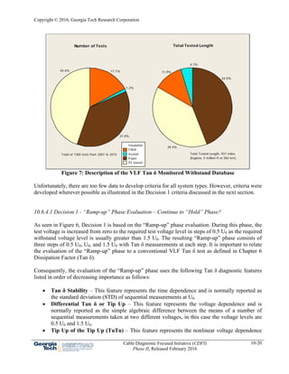
Subsequently, the criteria for test time amendment for all insulation types are shown in Table 8
through Table 10.
Table 8: CDFI Research Criteria for Time Amendment of the “Hold” Phase of PE-based
Insulations
(i.e. PE, HMWPE, XLPE, & WTRXLPE)*
Decision 2 – Amend Test Time?
“Hold” Phase Evaluation
[E-3]
“Reduce to 15 min” “Extend to 60 min”
Absolute
Change in Tan δ
ǀTD10-TD0ǀ
<0.6 >8
and or
Tan δ Stability
(Standard Deviation – STD10)
<0.3 >5
and or
Tan δ Level
(Mean Tan δ – TD10)
<14 >70

10-28
* Based on data as described in Table 4
Table 9: CDFI Research Criteria for Time Amendment of the “Hold” Phase of Filled
Insulations
(i.e. EPR & Vulkene)*
[E-3]
Absolute
Change in Tan δ
ǀTD10-TD0ǀ
<0.6 >6
and or
Tan δ Stability
<0.3 >5
and or
Tan δ Level
<13 >105
Table 10: CDFI Research Criteria for Time Amendment of the “Hold” Phase for Paper
Insulations
(i.e. PILC)*
[E-3]
Absolute
Change in Tan δ
ǀTD10-TD0ǀ
<1.4 >5
and or
Tan δ Stability
<0.6 >5.4
and or
Tan δ Level
<80 >180
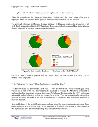
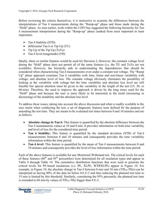
Using the above criteria, the expected outcomes for Decision 2 appear in Figure 11. These results
are used in the case studies that appear in Section 10.6.4.4.

10-29
Figure 11: Outcomes for Decision 2 Using CDFI Research Data – Amend Test Time?
If the segment under test successfully completes the “Hold” phase without a FOT, then the final
step is to provide a condition assessment. The details of how this assessment is conducted are
described in the next section.
10.6.4.3 Decision 3 – “Hold” Phase Evaluation – Final Assessment?
Once a VLF Tan δ monitored withstand test has concluded without a FOT, a final evaluation of the
“Hold” phase data is required. The utility engineer must then confront a condition assessment that
involves a multitude of potential features. This is represented in Figure 6 as Decision 3 – Final
Assessment. This assessment can be accomplished by estimating a qualitative “Pass” margin that is
derived from diagnostic features obtained from the “Hold” phase. The “Pass” margin is useful to
classify cable systems into three categories or classes:
 “No Action Required” – Systems in this category are assumed to have aa adequate“Pass”
margin and are not expected to fail in the near future. Failures, if any, are expected to appear
months or years after testing. Therefore, systems can be returned to service without any
major concerns.
 “Action Required” – Systems in this category are assumed to have a poor/low “Pass”
margin and if no action is taken and these systems are returned to service, failures are
expected to appear in the near future minutes to days after testing. Actions following an
“Action Required” assessment should include placing the cable system on a “watch list” and
considering replacement in the near future.
 “Further Study” – This category covers systems in which a clear evaluation of the “Pass”
margin cannot be accomplished. Therefore, a final condition assessment is not
straightforward. However, actions following a “Further Study” class may aid in finding a
final assessment and are described below.
61.0%
10.0%
29.0%
70.5%
6.8%
22.8%
54.4%
9.7%
35.9%
PE-Based Filled
Paper
Reduce to 15 min
Continue as planned to 30 min
Extend to 60 min
Decision 2

10-30
Cable systems with an evaluation of the “Hold” phase resulting in “Further Study” may require
remedial actions in the near future that should be sequentially undertaken as follows:
 review data for a rogue measurement in the sequence – most common during the first few
voltage cycles
 confirm insulation type to ensure that criteria apply
 verify the integrity of the terminations and if compromised, clean or replace them and repeat
the test
 retest in the near future and observe trends (6 months to a year) or
 place on “watch list” and consider system replacement in the near future
The estimation of the “Pass” margin is not a simple process. The diagnostic features needed to
evaluate the “Hold” phase must first be determined and then considered together for the final
assessment. Fortunately, irrespective of insulation type, the features can be determined by Cluster
Variable Analysis (CVA) [16] and then the grouping of features for the final assessment can be
accomplished by Principal Component Analysis (PCA) [16-17]. Both the cluster variable analysis
and the PCA are described in detailed in the Appendix A and Appendix B, respectively.
To develop the final assessment, a set of features that built upon those identified during the Tan δ
Ramp assessment (Decision 1) were examined. This set was more limited in terms of the types of
features (voltage dependence could not be used). As a result, the set used as a starting point for the
Cluster Variable and Principal Component Analysis the following feature set:
1. Tan δ Stability (STD) – This feature represents the time dependence and is reported as the
standard deviation of sequential measurements at the particular test voltage level irrespective
of it is a 15, 30, or 60 min test.
2. Initial Tan δ (Init TD) – This feature represents the initial measured loss level at the
beginning of the “Hold” phase irrespective of it is a 15, 30, or 60 min test.
3. Final Tan δ (Final TD) – This feature represents the final measured loss level at the end of
the “Hold” phase irrespective of it is a 15, 30, or 60 min test.
4. Level of Tan δ (Mean TD) – This feature represents the average level of loss over the full
“Hold” phase irrespective of it is a 15, 30, or 60 min.
5. Speed (rate of change over time) of Tan δ between 0 and 5 min (SPD 0-5) – This feature
represents an estimate of the rate of change in time of the loss level (Tan δ) during the first 5
minutes of the “Hold” phase. More importantly, this feature also provides information about
the trend of the measurements during the period under consideration; i.e. positive values
indicate an increasing trend and vice versa.
6. Speed of Tan δ between 5 and 10 min (SPD 5-10) – This feature represents an estimate of
the rate of change in time of the loss level (Tan δ) during the second 5 minutes of the “Hold”
phase.
7. Speed of Tan δ between 10 and 15 min (SPD 10-15) – This feature represents an estimate
of the rate of change in time of the loss level (Tan δ) during the third 5 minutes of the
“Hold” phase.
8. Speed of Tan δ Between 0 and final test time (SPD 0-tfinal) – This feature represents an
estimate of the overall rate of change of the loss level (Tan δ) with time for a completed
“Hold” phase irrespective of it is a 15, 30, or 60 min test.

10-31
An example of measured data during the “Hold” phase with the previously described diagnostic
features appears in Figure 12.
302520151050
80
70
60
50
40
30
20
10
0
Time [min]
TD[E-3]
1. Tan d Stability (STD)
2. Initial Tan d (Init TD)
(Final TD)
3. Final Tan d
4. Level of Tan d (Mean TD)(SPD 0-5)
Between 0 and 5 min
5. Speed of Tan d
(SPD 5-10)
Between 5 and 10 min
6. Speed of Tan d
(SPD 10-15)
Between 10 and 15 min
7. Speed of Tan d
(SPD 0-tfinal)
Between 0 and Final Test Time
8. Speed of Tan d
Figure 12: Example of Real Measured Tan δ data and Diagnostic features from a PE Cable
System during the “Hold” Phase
As described above, eight features are available for determining the appropriate assessment class.
Cluster Variable Analysis (reduces the feature set) and Principal Component Analysis (finds the
best combination of features) were used to identify which features to include in the condition
assessment. This was done for all three insulation classes (PE-based, filled, and PILC). The details
of this feature reduction/identification are discussed in Appendix C, Appendix D, and Appendix E
for PE-based, filled, and PILC, respectively. The remaining discussion in this section focuses on the
results of these analyses.
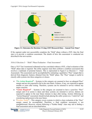
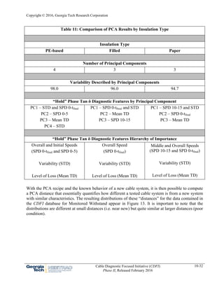
Table 11 shows the “recipes” that result from completing the CVA and PCA for each of the
insulation types. As this table shows, the features and their positions within the principal
components change depending on the insulation type.

10-32
Table 11: Comparison of PCA Results by Insulation Type
Insulation Type
PE-based Filled Paper
Number of Principal Components
4 3 3
Variability Described by Principal Components
98.0 96.0 94.7
“Hold” Phase Tan δ Diagnostic Features by Principal Component
PC1 – STD and SPD 0-tfinal
PC2 – SPD 0-5
PC3 – Mean TD
PC4 – STD
PC1 – SPD 0-tfinal and STD
PC2 – Mean TD
PC3 – SPD 10-15
PC1 – SPD 10-15 and STD
PC2 – SPD 0-tfinal
PC3 – Mean TD
“Hold” Phase Tan δ Diagnostic Features Hierarchy of Importance
Overall and Initial Speeds
(SPD 0-tfinal and SPD 0-5)
Variability (STD)
Level of Loss (Mean TD)
Overall Speed
(SPD 0-tfinal)
Variability (STD)
Middle and Overall Speeds
(SPD 10-15 and SPD 0-tfinal)
Variability (STD)
With the PCA recipe and the known behavior of a new cable system, it is then possible to compute
a PCA distance that essentially quantifies how different a tested cable system is from a new system
with similar characteristics. The resulting distributions of these “distances” for the data contained in
the CDFI database for Monitored Withstand appear in Figure 13. It is important to note that the
distributions are different at small distances (i.e. near new) but quite similar at larger distances (poor
condition).

10-33
1001010.10.01
99.9
99
90
80
70
60
50
40
30
20
10
5
3
2
1
PCA Distance - Arbitrary Units
Percentage[%] 95
80
PE - based
Filled
Paper
Type
Insulation
Figure 13: Comparison of Empirical Cumulative Distributions of the PCA Distance used for
Evaluation of the “Hold” Phase by Insulation Type
Figure 13 also shows the typical thresholds that were used throughout CDFI research and so these
define the separations from the different assessment classes for each insulation type. “Action
Required” (> 95%) is virtually the same for each of the insulations. There is a more pronounced
difference at the “Further Study” threshold (80%). Results from Figure 13 and Table 11 provide
indications that when the PCA results are considered together, there are issues to be imparted for all
insulation types. These issues appear below:
 The number of diagnostic features used to describe the “Hold” phase can be reduced to four
or five features. These features cover more than 95% of the data variability.
 The type and importance of the diagnostic features is generally the same regardless of the
insulation type; speeds are the more important features, followed by the variability, and the
level of loss.
 The differences observed in the PCA distances (Figure 13) strongly suggest that valuable
knowledge of VLF Tan δ Monitored Withstand is gained from collating experience.
Furthermore, it shows that the data must be collected separately for different insulation
types.
The following section illustrates the use of these results in case studies.

10-34
10.6.4.4 Case Studies
To improve the understanding of the application of the VLF monitored withstand framework, this
section presents examples of how the framework is deployed using real data from the field.
 Case Study 1: Data for a service-aged XLPE cable system that has been assessed by the
framework as “Further Study” at the end of the ramp, but test ultimately curtailed to 15 min.
 Case Study 2: Data for a service-aged XLPE cable system that has been assessed by the
framework as “Further Study” at the end of the ramp, but test ultimately extended to 30 min.
In both cases, the VLF monitored withstand data are presented graphically in Figure 14 and Figure
15 and the results of employing the Monitored Withstand framework appear in Table 12 and Table
13, respectively.
151050-5
15
14
13
12
11
10
9
8
Time [min]
TD[E-3]
0.50
1.00
1.50
2.22
Uo [pu]
Phase
"Ramp-up"
Phase
"Hold"
Continue to "Hold" Phase?
Decision 1
Amend Test Time?
Decision 2
Final Assessment?
Decision 3
Test voltages according to IEEE Std. 400.2 - 2013
XLPE - 750 MCM - 15 kV - 2800 ft Cable System
Figure 14: Case Study 1: Field VLF Tan δ Monitored Withstand Data for a Service Aged
XLPE Cable System Ultimately Assessed as “No Action”

10-35
Framework for a Service Aged XLPE Cable System Assessed as “No Action”
(Tan δ from Figure 14)
Decisions Made On Site
Decision 1 – “Ramp-up” Phase Evaluation – Continue to “Hold” Phase?
Diagnostic
Feature
STD
[E-3]
TU
[E-3]
TuTu
[E-3]
TD
[E-3]
Feature Value 0.01 0.3 0.1 10.70
Assessment based on the criteria presented in Table 5
Individual
Feature
Assessment
“No” “No” “No” “Yes”
Overall Feature
Assessment
“Yes”
Decision 2 – “Hold” Phase Evaluation – Amend Test Time?
Diagnostic
Feature
ǀTD10-TD0ǀ
[E-3]
STD10
[E-3]
Mean TD10
[E-3]
Feature Value 0.1 0.05 11.4
Individual
Feature
Assessment
“Reduce to 15 min” “Reduce to 15 min” “Reduce to 15 min”
Overall Feature
Assessment
“Reduce to 15 min”
Decision Taken After Test
Decision 3 – “Hold” Phase Evaluation – Final Assessment?
Feature
SPD 0-5
[E-3/min]
SPD 5-10
[E-3/min]
SPD 0-tfinal
[E-3/min]
STD
[E-3]
Mean
Tan δ
[E-3]
PCA
Distance
Percentage
Rank
[%]
Feature Value 0.002 0.002 0.002 0.010 11.00 0.12 64.00
Assessment Based on Health Index from PCA (Table 18 and Figure 23)
Overall Feature
Assessment
“No Action”

10-36
6050403020100-10
100
80
60
40
20
0
Time [min]
TD[E-3]
0.50
1.00
1.50
1.75
Uo [pu]
Phase
"Ramp-up"
Phase
"Hold"
Continue to "Hold" Phase?
Decision 1
Amend Test Time?
Decision 2
Final Assessment?
Decision 3
XLPE - 1/0 AWG - 20 kV - 840 ft Cable System
Test voltages according to IEEE Std. 400.2 - 2013
Figure 15: Case Study 2: Field VLF Tan δ Monitored Withstand Data for a Service Aged
XLPE Cable System Ultimately Assessed as “Further Study”

10-37
Framework for a Service Aged XLPE Cable System Assessed as “Further Study”
(Tan δ from Figure 15)
Decisions Taken On Site
Decision 1 – “Ramp-up” Phase Evaluation – Continue to “Hold” Phase?
Diagnostic
Feature
STD
[E-3]
TU
[E-3]
TuTu
[E-3]
TD
[E-3]
Feature Value 0.10 19.00 2.80 20.70
Individual Feature
Assessment
“Yes” “Yes” “No” “Yes”
Overall Feature
Assessment
“Yes”
Decision 2 – “Hold” Phase Evaluation – Amend Test Time?
Diagnostic
Feature
ǀTD10-TD0ǀ
[E-3]
STD10
[E-3]
Mean TD10
[E-3]
Feature Value 26.40 12.70 55.0
Individual Feature
Assessment
“Extend to 60 min” “Extend to 60 min” “Extend to 30 min”
Overall Feature
Assessment
“Extend to 60 min”
Decision Taken After Test
Decision 3 – “Hold” Phase Evaluation – Final Assessment?
Feature
SPD 0-5
[E-3/min]
SPD 5-10
[E-3/min]
SPD 0-tfinal
[E-3/min]
STD
[E-3]
Mean
Tan δ
[E-3]
PCA
Distance
Percentage
Rank
[%]
Feature Value 1.98 3.30 0.47 8.20 68.70 1.44 93.50
Assessment Based on Health Index from PCA (Table 18 and Figure 23)
Overall Feature
Assessment
“Further Study”
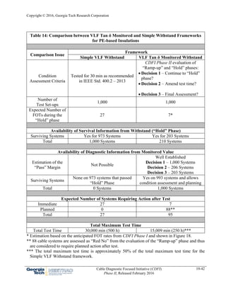
10.6.4.5 Comparison with Simple VLF Withstand
The previous sections have focused on the implementation and interpretation of the Monitored
Withstand test. However, the question remains what additional benefit a user gets for the added
complication implicit in the Monitored Withstand approach. It is, therefore, useful to compare the
monitored withstand framework with its Simple VLF Withstand counterpart in terms of inputs
(time) and outputs (subsequent actions). The comparison produces some unintuitive results that are

10-38
worth exploring. This section provides such a comparison assuming that the same group of cable
systems was assessed by both Simple and Monitored Withstand frameworks.
Assume that the test population has the following characteristics:
 1,000 Aged XLPE cable systems
 the average length of a cable system/segment is 1,000 ft
 anticipated FOT rates during the “Hold” phase correspond to the ones estimated during
CDFI Phase I (2.7% of 1,000 ft segments)
Figure 16 shows the estimated “Hold” phase performance of the Simple Withstand program. In
total, 1,000 withstand tests are performed for 30 min each. This produces 27 FOTs corresponding
with a failure rate of 2.7 %.
Figure 16: Simple VLF Withstand Framework on the Basis of Number of Tested Cable
Systems and Test Time for PE-based Insulations
Performance estimates for the Monitored Withstand framework for this set of cable systems appear
in Figure 17. In this case, the number of tested systems (blue solid line) declines significantly as a
result of Decision 1 (702 “No Action Required” and 88 “Action Required”). This implies that only
210 cable systems proceed to start the “Hold” phase. Stepping back to Decision 1 for this example,
it is important to remember that there are two potential implementations of Decision 1:
a) Only “Further Study” (“Amber Yes”) systems are considered to move forward to the “Hold”
phase or,

10-39
b) Both “Further Study” (“Amber Yes”) and “Action Required” (“Red No”) systems are
considered to move forward to the “Hold” phase.
In the example presented here, the implementation described in (a) above is the one that is
considered using the CDFI criteria presented in Table 5 to Table 7.
Figure 17: Monitored VLF Withstand Framework on the Basis of Number of Tested Cable
Systems and Test Time for PE-based Insulations
Figure 17 follows the 210 cable systems that enter the “Hold” phase after passing Decision 1. After
the first 15 min, there will have been on average four failures. At this point (Decision 2), 124 of
these systems can stop their respective withstand tests while the remaining 82 cable systems must
continue. As the systems reach the 30 min point, two cable systems will experience dielectric
failures and an additional 59 cable systems will be in position to end their withstand tests. The
remaining 21 cable systems will continue to 60 min with one system failing before 60 min. It is
worth examining some of these steps in more detail and compare them with the Simple Withstand
framework, Figure 18 shows the comparison between Simple VLF (Red) and VLF Tan δ Monitored
(Blue) withstand frameworks on the basis of number of tested cable systems and test time for PE-
based insulations.

10-40
Figure 18: Comparison between Simple VLF (Red) and VLF Tan δ Monitored (Blue)
Withstand Frameworks on the Basis of Number of Tested Cable Systems and Test Time for
PE-based Insulations
Interpretation of Figure 18 reveals that there are considerable differences in how the number of
tested systems changes as each framework evolves over test time. In particular, note for the
Monitored Withstand framework that the number of tested systems that actually go on to the “Hold”
phase is considerably reduced by the diagnostic selection made by Decision 1. A similar effect on
the number of tested segments can also be observed at 15 min during the “Hold” phase where again
the number of tested systems is considerably reduced by Decision 2. The reduced number of tested
segments can have a considerable impact on the total test time of the complete Monitored Withstand
test program when compared to a Simple Withstand approach. It is also important to mention that
since the number of tested systems is reduced during the test there is also an impact on the number
of FOTs and consequently the required emergency actions. In this context, immediate remedial
actions refer to actions needed to be undertaken to repair a system that has had a FOT.
The comparison shown in Figure 18 has also been performed for filled and paper insulations and
includes additional details such as:
 condition assessment criteria
 number of test set-ups
 expected number of FOTs during the “Hold” phase
 expected number of systems requiring immediate action
 expected number of systems requiring action on a planned basis
 estimation of the “Pass” margin

10-41
 availability of diagnostic information on surviving systems and
 total maximum test times are selected for comparison
Table 14, Table 15, and Table 16 show the comparisons for PE-based, filled, and PILC cable
systems, respectively.
As seen in Table 14, the VLF Tan δ Monitored Withstand framework improves upon all aspects of
the Simple VLF Withstand framework. In particular, the Monitored Withstand approach leads to a
reduction in the total required test time (30,000 min (500 h) versus 15,009 min (250 h)). This
represents a 50% reduction in the required time. In addition, the number of systems that require
immediate or planned action is 95 (7 immediate and 88 planned) for Monitored Withstand as
compared to 27 immediate actions for Simple Withstand. This can be viewed a number of ways but
is not unexpected since the Monitored Withstand framework classifies systems with unusual
estimated “Pass” margins as systems that require action on a planned basis. It is somewhat utility
dependent as to the relative importance of immediate and planned actions.
Table 15 shows a similar difference when Monitored Withstand and Simple Withstand are
employed on a set of filled cable systems.

10-42
Table 14: Comparison between VLF Tan δ Monitored and Simple Withstand Frameworks
for PE-based Insulations
Comparison Issue
Framework
Simple VLF Withstand VLF Tan δ Monitored Withstand
Condition
Assessment Criteria
Tested for 30 min as recommended
in IEEE Std. 400.2 – 2013
CDFI Phase II evaluation of
“Ramp-up” and “Hold” phases:
 Decision 1 – Continue to “Hold”
phase?
 Decision 2 – Amend test time?
 Decision 3 – Final Assessment?
Number of
Test Set-ups
1,000 1,000
Expected Number of
FOTs during the
“Hold” phase
27 7*
Availability of Survival Information from Withstand (“Hold” Phase)
Surviving Systems Yes for 973 Systems Yes for 203 Systems
Total 1,000 Systems 210 Systems
Availability of Diagnostic Information from Monitored Value
Estimation of the
“Pass” Margin
Not Possible
Well Established
Decision 1 – 1,000 Systems
Decision 2 – 206 Systems
Surviving Systems
None on 973 systems that passed
“Hold” Phase
Yes on 993 systems and allows
condition assessment and planning
Total 0 Systems 1,000 Systems
Expected Number of Systems Requiring Action after Test
Immediate 27 7
Planned 0 88**
Total 27 95
Total Maximum Test Time
Total Test Time 30,000 min (500 h) 15,009 min (250 h)***
* Estimation based on the anticipated FOT rates from CDFI Phase I and shown in Figure 18.
** 88 cable systems are assessed as “Red No” from the evaluation of the “Ramp-up” phase and thus
are considered to require planned action after test.
*** The total maximum test time is approximately 50% of the total maximum test time for the
Simple VLF Withstand framework.

10-43
for Filled Insulations
Comparison Issue
Framework
Condition
Assessment Criteria
in the IEEE Std. 400.2 – 2013
CDFI Phase II Project evaluation
of “Ramp-up” and “Hold” phases:
phase?
Number of
Test Set-ups
1,000 1,000
Expected Number of
FOTs during the
“Hold” phase
27 7*
Estimation of the
“Pass” Margin
Not Possible
Well Established
Surviving Systems
None on 973 systems that passed
“Hold” Phase
Immediate 27 7
Planned 0 84**
Total 27 91
* Estimation based on the anticipated FOT rates from the CDFI Phase I and shown in Figure 18.
Table 16 illustrates that paper systems have somewhat unique differences as compared to either

10-44
extruded insulation type.
for Paper Insulations
Comparison Issue
Framework
Condition
Assessment Criteria
in the IEEE Std. 400.2 – 2013
CDFI Phase II Project evaluation
of “Ramp-up” and “Hold” phases:
phase?
Number of
Test Set-ups
1,000 1,000
Expected Number of
FOTs during the
“Hold” phase
27 12*
Estimation of the
“Pass” Margin
Not Possible
Well Established
Surviving Systems No for 973 Systems
Immediate 27 12
Planned 0 67**
Total 27 79
* Estimation based on the anticipated FOT rates from the CDFI Phase I and shown in Figure 18.

10-45
Finally, a comparison between VLF Tan δ Monitored Withstand frameworks between insulation
types is shown in Table 17 based on the expected number of condition assessment decisions on site
and after test, expected number of systems requiring action after test, and total maximum test time
for the test program example considered in this section.
Table 17: Comparison between VLF Tan δ Monitored Frameworks Including all
Insulation Types
Comparison Issue PE-based Filled Paper
Expected Number of Condition Assessment Decisions
On Site
Decision 1
Continue to “Hold” phase?
1,000 1,000 1,000
Decision 2
Amend test time?
206 279 354
After Test
Decision 3
Final Assessment?
203 276 349
Immediate 7 7 12
Planned 88 84 67
Total 95 91 79
Total Test Time 15,009 min (250 h) 16,105 min (268 h) 18,940 min (316 h)
Relative to a Simple
Withstand Framework
50% 54% 63%
10.6.5 Monitored Withstand Using Partial Discharge
The quantities of field data provided or gathered where PD is the monitored property for the
Monitored Withstand test were not sufficient for developing condition assessment decisions. While
technically feasible, the actual implementation of such a program, confirmed by CDFI
tests/experience, is complicated by the intrinsic difficulties of the PD test setup and analysis (see
Chapter 7 and Chapter 8 for details on PD testing). As a result, although conceptually possible, the
CDFI has not developed a perspective on this technique. Additional suggestions are discussed in
Section 10.7.1.

10-46
10.6.6 Monitored Withstand with Damped ac (DAC) Voltage Sources
Damped ac voltage sources have often been mentioned in the industry for use in withstand testing.
However, as DAC has proven ineffective for withstand tests (see Section 10.6.1); then the
inadvisability of DAC voltage sources for monitored withstand tests becomes evident.
Therefore, at the present time, DAC voltage sources do not meet the definition of a withstand test
(Simple or Monitored) and thus are not recommended. Field data are needed to show the pass and
fail capability and to provide evidence for the third element that defines a withstand test.
10.6.7 Monitored Withstand Using DC Leakage Current
Leakage Current data are primarily gathered during withstand tests utilizing dc voltage sources. The
use of dc withstand tests for aged-cable extruded cable systems has been highly discouraged for the
last two decades because of the accumulated space charge and its impact on system performance
once the cable system is re-energized with 60 Hz. At least one utility continued to utilize dc for its
withstand program during the CDFI and recorded some leakage current data. These data were
limited in scope and thus could not be analyzed in the same manner as the available VLF Tan δ
data. As a result, the CDFI has not developed a perspective on this technique. Additional
suggestions are discussed in Section 10.7.1.
10.7 Outstanding Issues
Monitored Withstand came into existence during the term of the CDFI research and so is one of the
“younger” techniques available. As such, there remain a number of outstanding issues of which the
more important are discussed below.
10.7.1 Monitored Withstand Framework – PD and Leakage Current
During the CDFI Phase II, it was not possible to collect enough data for PD and dc leakage current
during a Monitored Withstand test to properly establish a framework for these two monitored
properties. However, the CDFI perspective considers that it is likely that, the hierarchy observed
and confirmed by data from Monitored Withstand programs employing dielectric loss
measurements, could be generalized for any other monitored property. This is due to the fact that all
the levels of the monitored property hierarchy are logically correlated with system performance (i.e.
steeper trends, bigger variability, and increased absolute magnitude of the monitored property all
should indicate poorer cable system condition). Therefore, the hierarchy for PD and Leakage
Current could be conceptualized as follows:
1. Trends within the monitored period. These are likely to be categorical attributes: flat,
upward trend, downward trend, etc. They can also be characterized by speeds (e.g. average
change per unit time of the monitored property for a pre-established period within the test
time.).

10-47
2. Stability or scatter of the monitored property for a pre-established period within the test
time.
3. Absolute level of the monitored property for a pre-established period within the test time.
Therefore, the Monitored Withstand frameworks for PD and Leakage Current remain as open issues
that may be addressed by future research programs.
10.7.2 Criteria Based on Local and Global Data
The criteria for VLF Tan δ Monitored Withstand as well as those developed for other diagnostic
techniques are intended, by the nature of this project, to be industry-wide criteria that include test
results from as many utilities as possible. This provides a global perspective on each diagnostic
technique. This perspective does not distinguish between the variety of system designs,
environmental conditions, and installation practices used by the utilities supplying the data. The
result is a large dataset that represents the experience of many utilities. At present, criteria are
segregated only by insulation type.
Unfortunately, there could be cases where the criteria cannot be ideally applied to a particular case
of an individual utility. Indeed, this is specifically recognized in IEEE Std. 400.2 – 2013 where a
local utility perspective is advocated. This is due to the many factors that can contribute to system
aging such as the manufacturer, vintage, cable/accessory design, operating environment, and
operating conditions. In such cases, it would be necessary to generate local data and thus criteria
that are based solely on an individual utility’s cable system.
The process of developing local criteria is the same as that used to determine global criteria within
CDFI (see previous quarterly reports and the CDFI Phase I final report for more information). The
challenge is having enough data from the specific utility to facilitate this process. Therefore, local
criteria cannot be developed unless a significant effort is expended during the test. A utility just
starting a diagnostic program must rely on the global criteria until they can generate enough data for
local criteria to be useful.

10-48
10.8 References
1. P. Mohaupt, M. Baur, and T. Schlick, “VLF Testing and Diagnosis on Medium Voltage
Power Cables,” IEEE 10th
Inter. Conf. on Transmission and Distribution Construction,
Operation, and Live Line Maintenance, pp. 202-209, Apr. 2003 IEEE ESMO.
2. C. Goodwin, “Practical Smart Withstand Programs for MV Cable Systems,” IEEE Insulated
Conductors Committee, Subcommittee F Spring 2010.
3. P. Werelius, P. Tharning, R. Eriksson, B. Holmgren, and U. Gafvert, “Dielectric
Spectroscopy for Diagnosis of Water Tree Deterioration in XLPE Cables,” IEEE Trans. on
Dielectrics and Electrical Insulation, vol. 8, no. 1, pp 27-42, Mar 2001.
4. R.N. Hampton, R. Harley, R. Hartlein, and J. C. Hernández, “Practical Issues Regarding The
Use Of Dielectric Measurements To Diagnose The Service Health Of MV Cables,”
International Conference on Insulated Power Cables; JICABLE07, Versailles France, June
2007.
5. J. C. Hernández-Mejía, R. G. Harley, R. N. Hampton, and R. A. Hartlein, “Characterization
of Ageing for MV Power Cables Using Low Frequency Tan-delta Diagnostic
Measurements,” IEEE Transactions on Dielectrics and Electrical Insulation, Vol. 16, Issue
3, pp. 862-870, June 2009.
6. J. Perkel, Y. Del Valle, R. N. Hampton, J. C. Hernández-Mejía, and J. Densley,
“Interpretation of Dielectric Loss Data on Service Aged Polyethylene Based Power Cable
Systems using VLF Test Methods,” Accepted for publication on the IEEE Transactions on
Dielectrics and Electrical Insulation.
7. J. C. Hernández-Mejía, J. Perkel, R. Harley, N. Hampton, and R. Hartlein, “Correlation
between Tan δ Diagnostic Measurements and Breakdown Performance at VLF for MV
XLPE Cables,” IEEE Trans. on Dielectrics and Electrical Insulation, February 2009, pp.
162-170.
8. R. N. Hampton, R. Harley, R. Hartlein, and J. C. Hernández, Practical Issues Regarding The
Use Of Dielectric Measurements To Diagnose The Service Health Of MV Cables,
International Conference on Insulated Power Cables; JICABLE07, Versailles France, June
2007.
9. H. R. Gnerlich, “Field Testing of HV Power Cables: Understanding VLF Testing,” IEEE
Electrical Insulation Magazine, vol. 11, no. 5, pp. 13–16, Sep./Oct. 1995.
10. S. C. Moh, “Very low frequency testing - Its effectiveness in detecting hidden defects in
cables,” 2003 CIRED (17th International Conference on Electricity Distribution), Barcelona,
Paper 84, May 12–15, 2003.
11. R. N. Hampton, J. Altamirano, J. Perkel, and J. C. Hernandez, “VLF Tests Conducted by
NEETRAC as Part of the CDFI,” IEEE Insulated Conductors Committee, Fall 2007
Meeting, Scottsdale AZ, 2007.
12. R. N. Hampton, J. Perkel, J. C. Hernandez,, M. Begovic, J. Hans, R. Riley, P. Tyschenko, F.
Doherty, G. Murray, L. Hong, M. G. Pearman, C. L. Fletcher, and G. C. Linte, “Experience
of Withstand Testing of Cable Systems in the USA,” CIGRE 2010, Paper No. B1-303.
13. C. Goodwin, H. Oetjen, and M. Peschel, “Use of VLF Methods in Utility Reliability
Programs - Basic Concepts,” IEEE Insulated Conductors Committee, Subcommittee F, Fall
2009 Meeting, Scottsdale AZ, 2009.
14. J. Perkel, J. Altamirano, and N. Hampton, “Investigation of VLF Test Parameters,” IEEE
Insulated Conductors Committee, Subcommittee F, Spring 2010 Meeting, Nashville, TN,

10-49
2010.
15. IEEE, “IEEE Guide for Field Testing of Shielded Power Cable Systems Using Very Low
Frequency (VLF) (less than 1 Hz),” IEEE Std. 400.2 – 2013, Jun. 2013.
16. R. Duda, P. Hart, and D. Stork, “Pattern Classification,” Second Edition, John Wiley &
Sons, Inc., New York, 2000, ISBN 0-471-05669-3.
17. Box G. E. P., Hunter W. G., and Hunter J. S., Statistics for Experimenters, John Wiley &
Sons, Inc., New York, NY, USA, 2nd
Edition, 2005, ISBN-100-471-71813-0.

10-50
10.9 Relevant Standards
 IEEE Std. 400 – 2012: IEEE Guide for Field Testing and Evaluation of the Insulation of
Shielded Power Cable Systems Rated 5 kV and Above
 IEEE Std. 400.1 – 2007: IEEE Guide for Field Testing of Laminated Dielectric, Shielded
Power Cable Systems Rated 5 kV and Above With High Direct Current Voltage
 IEEE Std. 400.2 – 2004: IEEE Guide for Field Testing of Shielded Power Cable Systems
Using Very Low Frequency (VLF)
 IEEE Std. 400.2 – 2013: IEEE Guide for Field Testing of Shielded Power Cable Systems
Using Very Low Frequency (VLF) (less than 1 Hz)
 IEEE Std. 400.3™ – 2006: IEEE Guide for Partial Discharge Testing of Shielded Power
Cable Systems in a Field Environment
 IEEE Std. 400.4™ – 2014: Omnibus - IEEE Draft Guide for Field-Testing of Shielded
Power Cable Systems Rated 5kV and Above with Damped Alternating Current Voltage
(DAC)
 IEEE Std. 404™ – 2006: IEEE Standard for Extruded and Laminated Dielectric Shielded
Cable Joints Rated 2500 V to 500 000 V

10-51
10.10 Appendix
10.10.1 Details of Feature Elimination Using Cluster Variable Analysis
One of the problems that occur when considering a large number of Tan δ diagnostic features is
how to organize these features (stability, changes with time/voltage at various levels, and
magnitudes) into meaningful groups or clusters. Cluster variable analysis is useful because it
identifies key variables that explain the principal dimensionality (not variability) of the data. It is
used to classify the data into groups when the groups are initially unknown. One important reason to
cluster the variables is to reduce their number but, more importantly, it is used in this research to
understand the taxonomy and meaning of the Tan δ diagnostic features.
The analysis is an agglomerative hierarchical method that begins with a separate treatment of all
features, each forming its own cluster. In the initial step, the two features closest together are joined.
In the next step, either a third feature joins the first two (now considered as a stand-alone cluster) or
another feature is joined with a different cluster. This process continues until all clusters are joined
into one. The complete process, from the initial cluster variable analysis to the final feature
selection, is explained later in the chapter for all insulation types.
The agglomerative hierarchical method uses the distances between variables when forming the
clusters. These distances are based on a single dimension that uses the absolute Pearson correlation
coefficient [17] between features. The correlation coefficient can be translated to a level of
similarity between clusters. The level of similarity can be used as a tool to compare the relationship
between features or clusters.
The similarity level between two features or clusters, e.g. features or clusters i and j, is given by the
following equation,
100 1
Equation 1
where,
Sij: Similarity level between features or clusters i and j,
dij: distance measure between features or clusters i and j, based on the absolute Pearson correlation
coefficient,
dmax: Maximum distance between the initial set of features before starting the clustering procedure.
The interpretation of the level of similarity is quite straightforward. The level of similarity is a
number that ranges from 0% to 100%. A similarity level approaching 100% indicates that the
features or clusters under investigation are redundant, i.e. they carry essentially the same
information. In other words, the features or clusters are highly correlated; thus, they contribute little
to solving an eventual classification problem. In contrast, a level of similarity approaching 0%
indicates that the features or clusters under investigation are complementary or uncorrelated. Thus,
the likelihood of using these features or clusters in an eventual classification problem with good

10-52
results is higher than using redundant features or clusters.
There are several algorithms available for the clustering of the Tan δ diagnostic features and each of
them may yield different results. However, here, the group average and the furthest neighbor
methods are used in the cluster variable analysis of the Tan δ diagnostic features. Specifically, the
group average method is used in the agglomerative procedure during clustering. The clustering
process is as follows:
1. Initially each feature is declared a cluster and all distances between clusters are calculated.
2. Two clusters with the smallest distance between them are fused together and declared to be a
new cluster. This is the beginning of the agglomerative process.
3. All distances between clusters are again calculated and the agglomerative process continues
until the number of clusters is one.
4. Once one cluster is left, the number of clusters to be considered for the final feature
selection is determined by choosing a similarity level.
The results of the clustering procedure can be represented graphically in a tree-like plot, also known
as a dendrogram plot. The dendrogram plot for the cluster variable analysis represents the features
under analysis on the x-axis and the level of similarity between features and clusters on the y-axis.
The clusters are represented by vertical and horizontal lines between the features.
Determining the number of clusters for the final feature selection can be termed as “cutting the
dendrogram”. Cutting the dendrogram is akin to drawing a line across the dendrogram to specify the
final grouping at a particular similarity level. There is no pre-established procedure on choosing the
similarity level for cutting the dendrogram. However, a good similarity level to cut the dendrogram
is that level at which a sudden change in the number of initial clusters is observed.
Examples of dendrograms appear in Appendix C, D, and E.

10-53
10.10.2 Single Diagnostic Indicator Based on Principal Component Analysis (PCA)
Principal Component Analysis (PCA) is a method that combines diagnostic features to create a
single diagnostic indicator that puts any set of measurements in context with the “Hold” phase Tan
δ measurements database. Therefore, through the single diagnostic indicator, the “Pass” margin can
be estimated.
The PCA technique is useful because it takes a given set of points in a high dimensional space and
then reduces the dimensionality to a more manageable number. In other words, the PCA technique
summarizes the data with several assumed independent variables to a smaller set of derived
variables without sacrificing the potential for classification. In fact, the classification capability is
enhanced by the PCA [16-17].
The technique provides a predictive model with guidance on how to interpret or “weigh” the
primary measurement features. It also allows a physical meaning to be ascribed to the resulting
composite factors, i.e. the Principal Components. The PCA approach identifies linear combinations
of factors and generates the principal components that better represent the data. The first component
has or describes the largest portion of the variance, followed by the second, and then the third, and
so on. The PCA redistributes the variance in such a way that the first k components explain as much
as possible of the total variance of the data. It must be noted that the higher the variance the higher
the potential for better classification.
Another important reason for choosing the PCA technique is that in many data analysis/mining
scenarios, seemingly independent variables are highly correlated, which affects model accuracy and
reliability. PCA is able to detect such correlations and then essentially exclude the redundant
information; however, some of the redundancy has been previously filtered by the cluster variable
analysis discussed earlier.
To illustrate and easily understand the essentials of the PCA technique, Figure 19 shows a
qualitative explanation of the technique. The circles represent a dataset in which there are two
features (axes) and the variance within this dataset with respect to these features is represented by
the area of the rectangle denoted as Area 1. The PCA method attempts to reduce the variance by
generating new axes that are linear combinations of the available two features. This causes a
rotation/translation of the original axes from F1-F2 to PC1-PC2. The new variance can then be
thought of as the area of the rectangle represented by Area 2. Comparing the areas clearly shows
that area 2 is smaller and, therefore, has less variance than the original configuration in Area 1. As
mentioned above, this process reduces the dimension of a dataset to as few or as many principal
components as are needed.

10-54
Figure 19: Graphical Interpretation of Principal Component Analysis (PCA)
Once the dimensionality has been reduced, the selected principal components can be used to
compute a PCA distance from a known set of PCA transformed diagnostic features providing in this
way the single diagnostic indicator. The process to compute the single diagnostic indicator appears
in Figure 20.
Figure 20: Calculation of the Single Diagnostic Indicator from PCA
As seen in Figure 20, the known set of PCA transformed diagnostic features corresponds to features
of a new cable system and this allows for establishing a critical diagnostic for the single diagnostic
indicator and its corresponding “Pass” margin. In this case, the critical levels are also determined
using the Pareto Principle [17], for two critical levels at the 80th
and 95th
percentiles of the data. The
interpretation of the single diagnostic indictor based on PCA distance and its corresponding “Pass”
margin (Decision 3 on Figure 6) is as follows

10-55
:
 Cable systems showing a PCA distance bellow the 80th
percentile have a good “Pass”
margin and thus are classified as “No Action Required.”
 Cable systems showing a PCA distance between the 80th
and 95th
percentiles have an
uncertain “Pass” margin and thus are to be classified as “Further Study.”
 Cable systems showing a PCA distance beyond the 95th
percentile have a poor “Pass”
margin and thus are classified as “Action Required.”
The interpretation of the single diagnostic indicator based on PCA distance completes the picture of
the Monitored Withstand test framework using VLF Tan δ measurements and it is one of the more
important contributions of the CDFI. The next sections show results of the “Hold” phase evaluation
for all insulation types.
10.10.3 PE-Based Insulation Final Assessment
This appendix describes the analysis process employed on the available VLF Tan δ Monitored
Withstand data to develop criteria for making the condition assessment for PE-based cable systems.
Also discussed are the test cases used to validate the approach.
Results of the cluster variable analysis of the diagnostic features used to characterize the “Hold”
phase for PE-based insulations appear in Figure 21. As a reminder, the feature descriptions are also
below:
1. Tan δ Stability (STD) – This feature represents the time dependence and is reported as the
standard deviation of sequential measurements at the particular test voltage level irrespective
of it is a 15, 30, or 60 min test.
2. Initial Tan δ (Init TD) – This feature represents the initial measured loss level at the
beginning of the “Hold” phase irrespective of it is a 15, 30, or 60 min test.
3. Final Tan δ (Final TD) – This feature represents the final measured loss level at the end of
the “Hold” phase irrespective of it is a 15, 30, or 60 min test.
4. Level of Tan δ (Mean TD) – This feature represents the average level of loss over the full
“Hold” phase irrespective of it is a 15, 30, or 60 min.
5. Speed (rate of change over time) of Tan δ between 0 and 5 min (SPD 0-5) – This feature
represents an estimate of the rate of change in time of the loss level (Tan δ) during the first 5
minutes of the “Hold” phase. More importantly, this feature also provides information about
the trend of the measurements during the period under consideration; i.e. positive values
indicate an increasing trend and vice versa.
6. Speed of Tan δ between 5 and 10 min (SPD 5-10) – This feature represents an estimate of
the rate of change in time of the loss level (Tan δ) during the second 5 minutes of the “Hold”
phase.
7. Speed of Tan δ between 10 and 15 min (SPD 10-15) – This feature represents an estimate
of the rate of change in time of the loss level (Tan δ) during the third 5 minutes of the
“Hold” phase.
8. Speed of Tan δ Between 0 and final test time (SPD 0-tfinal) – This feature represents an

10-56
estimate of the overall rate of change of the loss level (Tan δ) with time for a completed
“Hold” phase irrespective of it is a 15, 30, or 60 min test.
Spd
0-5
(E-3/m
in)
S
pd
5-10
(E-3/m
in)
Spd
0-tfinal(E-3/m
in)
Spd
10-15
(E-3/m
in)
STD
(E-3)
Init TD
(E-3)
Fin
al TD
(E-3)
M
ean
TD
(E-3)
55.83
70.55
85.28
100.00
Diagnostic Features
SimilarityLevel[%]
Cluster 1
Cluster 2 Cluster 3 Cluster 4 Cluster 5
Selected Feature
Figure 21: Cluster Variable Analysis Results for PE-based Insulations
(Based on data as described in Table 4)
As Figure 21 shows, when a similarity level of approximately 85% is chosen to cut the dendrogram,
five clusters result:
 Cluster 1 – Mean TD, Final TD, and Init TD
 Cluster 2 – STD
 Cluster 3 – SPD 10-15 and SPD 0-tfinal
 Cluster 4 – SPD 5-10
 Cluster 5 – SPD 0-5.
In the approach presented here, each cluster may be represented by one single diagnostic feature
from within that cluster. The selection of the diagnostic feature to represent each cluster appears in
Figure 21 by the blue dashed lines and thus the final selected set of features is indicated by the blue
squares.
The cluster variable analysis results also provide insight into the types of features applicable for the
PCA as well as their relative importance. The assumption here is that features that are more
dissimilar may be more important. Following this logic, the more important features are the speeds
(clusters 3, 4, and 5); particularly at the beginning of the “Hold” phase when higher speed
magnitudes are generally observed, followed by the STD (cluster 2) and loss level (cluster 1). The
results of the cluster variable analysis shown in Figure 21 indicate that five of the initial set of eight
diagnostic features should be considered for the PCA.

10-57
PCA was applied to the “Hold” phase monitored withstand database of PE-based insulations. Figure
22 shows the transformation from two Tan δ diagnostic features (STD and SPD 0-tfinal) to the first
two principal components (PC1 and PC2). As mentioned previously, the PCA reduces the
dimensionality; however, this technique does not directly provide a single diagnostic indicator by
itself. It does enable the construction of simplified and appropriate feature maps that may enhance
the classification potential of the diagnostic features when they are appropriately combined. The
principal component feature maps provide a single condition assessment descriptor. The
transformation can be observed in Figure 22 in which the application of the PCA transformation
reveals a clearer connection between PC1 and PC2 (right side of Figure 22) as compared to the
original data (STD and SPD 0-tfinal shown on the left side of Figure 22).
24181260
2
1
0
-1
-2
-3
ST D (E-3)
Spd0-tfinal(E-3/min)
1.00.50.0-0.5
1.0
0.5
0.0
-0.5
-1.0
PC1 -> ST D and SPD 0-tfinal
PC2->SPD0-5
Figure 22: STD vs. SPD 0-tfinal (left) and PC1 vs. PC2 (right) – PE-based Insulations
Applying PCA to the full database yields the principal components shown in Table 18. This table
shows the percentage of variance accounted for by each principal component (i.e. the variability) as
well as the diagnostic features that contribute the most to each component. Results from Table 18
indicate that only four principal components are required to describe 98% of the data variance. It is,
therefore, reasonable to utilize four principal components.

10-58
Table 18: PCA Variances and Component Composition for PE-based Insulations
Principal
Component
Variance
Described by
Component
[%]
Cumulative
Variance
[%]
“Hold” Phase
Tan δ Diagnostic Features
PC1 49 49
STD and SPD 0-tfinal
(Variability and trend)
PC2 28 77
SPD 0-5
(Trend)
PC3 12 89
Mean TD
(Level of Loss)
PC4 9 98
STD
(Variability)
PC5 2 100 Not relevant
The main observation from the PCA results in Table 18 is that they also give an indication of the
importance and relevance of the “Hold” phase Monitored Withstand Tan δ diagnostic features. The
features can be ranked in importance as:
1. trend of the measurements (SPD 0-tfinal and SPD 0-5)
2. time dependence (STD) and
3. loss level (Mean TD)
The overarching question is - How to combine all diagnostic features into a single indicator?
The identification of suitable Principal Components also allows these components to be combined
together to form a set of coordinates. The approach adopted elsewhere within CDFI has been to
calculate the Euclidean distance between the data point and a reference point. The greater the
distance, the less like the reference point is to the newly acquired data point. Applying this principle
to these data, the best choice for a reference point is a new cable system. As a result, the distance
calculated essentially quantifies the gulf between a new cable system and an aged system.
Figure 23 shows the combined PCA distance of the four principal components for all the available
Monitored Withstand data from PE-based cable systems. If all the data are ranked from smallest
(most like new) to largest (least like new) this gives the rank position, which can easily be
converted to a percentage. In practice, the resulting graph might conveniently be regarded as the
“Pass” margins for the population of cable systems tested. The interpretation is straightforward as
the higher rank positions represent those cable systems that are least “like new” while the low rank
positions correspond to those systems that most “like new”.

10-59
1001010.10.010.001
99
95
90
80
70
60
50
40
30
20
10
Percentage[%]
95
80
1.80.4
“Hold” Phase for PE-based Cable Systems
Critical level for the single diagnostic indicator can be established using the same Pareto Principle
as before. The 80th and 95th percentage ranks appear in Figure 23 and they correspond to PCA
distances of 0.4 and 1.8, respectively. The critical levels for the single diagnostic indicator are then
used to establish the final condition assessment and thus address Decision 3, “Hold” Phase
evaluation, of the Monitored Withstand framework. The critical levels for the single diagnostic
indicator and corresponding condition assessment categories appear in Figure 24.
1001010.10.010.001
99
95
90
80
70
60
50
40
30
20
10
Percentage[%]
95
80
1.80.4
No Action
NA
Required
Action
AR
Study
Further
FS
“Hold” Phase for PE-based Cable Systems with Condition Assessment Categories

10-60
Several case studies using experimental data/features illustrate the application of the research PCA
to the evaluation of the “Hold” phase of a Monitored Withstand test. The summary of these case
studies appears in Table 19.
Table 19: Cases Studies for “Hold” Phase Evaluation for PE-based Insulations
Case
No.
Description
SPD 0-5
[E-3/min]
SPD 5-10
[E-3/min]
SPD 0-tfinal
[E-3/min]
STD
[E-3]
Mean
Tan δ
[E-3]
Percentage
Rank
[%]
1 New System 0.002 0.002 0.002 0.01 0.1 2.9
2
Features at 80% level
and Pos. Speeds *
0.350 0.350 0.350 15.00 0.3 76.0
3
and Neg. Speeds *
-0.350 -0.350 -0.350 15.00 0.3 74.0
4
and Pos. Speeds *
3.000 3.000 3.000 5.00 70.0 95.0
5
and Neg. Speeds *
-3.000 -3.000 -3.000 5.00 70.0 94.0
6 Utility Test 1 0.420 0.140 0.227 0.80 10.1 69.0
7 Utility Test 2 2.500 -0.480 0.067 5.20 6.3 89.0
8 Utility Test 3 3.960 2.480 1.460 23.10 200.0 96.0
* The 80% and 95% diagnostic feature levels correspond to level of the diagnostic features for
“Hold” phase” Evaluation – Decision 2 – Amend Test Time? as shown in Table 8 considering
constant speed values during the period under evaluation.
In Table 19, the following examples are included:
 Case 1: New PE cable system that lies within the 0.03st
percentile. This translates to an
extremely good “Pass” margin. Case 1 is represented in Figure 25 by the solid black circle
symbol.
 Case 2: All diagnostic features set to their respective 80% levels (black square symbol in
Figure 25) with positive speeds. It is important to note here that all the features at the 80%
level yield a percentage of 76.0%. Therefore, there is an acceptable correlation between the
feature levels and the overall assessment considering all features together.
 Case 3: All diagnostic features are at their respective 80% levels with negative speeds. In
this case all of the features set at the 80% level yield a percentage of 74.0%. Therefore, there
is again good correlation between the feature levels and the overall condition assessment.
 Case 4: All diagnostic features are set at their 95% levels (black triangle symbol in Figure
25) with positive speeds. In this case, the percentage is exactly 95.0%. Therefore, there is a
good correlation between the feature levels and the overall assessment considering all

10-61
features together.
 Case 5: All diagnostic features set at their 95% levels with negative speeds. In this case, the
percentage is 94.0%. Note again the good correlation between the features levels and the
overall condition assessment.
 Case 6: Real case and represents one of the low to mid performers. The PCA indicates that
in 2014 the cable system is within the upper “No Action” category with a rank of 69.0%.
 Case 7: Real case and represents one of the mid to high performer. The PCA indicates the
cable system is within the “Further Study” category with a rank of 89.0%.
 Case 8: Real case and represents one of the poorest performer in a cable system (black
diamond symbol in Figure 25). The PCA indicates that in 2013 the cable system is within
the poorest 4% of all PE-based cable systems.
The symbols in Figure 25 represent selected test cases used as examples and their computed PCA
distance (rank) results appear in Table 19.
1001010.10.010.001
99
95
90
80
70
60
50
40
30
20
10
Percentage[%]
95
80
New System - Case 1
All Features at 80% Level and Pos. Speeds - Case 2
Utility Test 2013 - Case 8
Figure 25: Empirical Cumulative Distribution of the PCA Distance from CDFI Research Used
for Evaluating the “Hold” Phase for PE-based Cable Systems with Relevant Case Studies
from Table 19
Observe that in Table 19 there are only small differences between the ranks of Cases 2 and 3 and
Cases 4 and 5. This is because the distance approach only considers the magnitude of the trend and
not its direction (i.e. positive speeds (not vectors) compared to negative speeds). At first glance, this
may be perceived as a disadvantage of the PCA distance approach. However, even though negative
trends (negative speeds) generally indicate better system conditions than systems with positive

10-62
trends (positive speeds) to date there is no theoretical nor experimental basis to support this belief,
however reasonable, for PE-based insulations.
10.10.4 Filled Insulation Final Assessment
This appendix describes the analysis process employed on the available VLF Tan δ Monitored
Withstand data to develop criteria for making the condition assessment for filled cable systems.
Also discussed are the test cases used to validate the approach.
Results of the cluster variable analysis of the diagnostic features used to characterize the “Hold”
phase for filled insulations appear in Figure 26. Note that the same feature set as was used in
Appendix A is used in Figure 26.
Spd
10-15
(E-3/m
in)
SPD
0-5
(E-3/m
in)
SPD
0-tfinal (E-3/m
in)
SPD
5-10
(E-3/m
in)
STD
(E-3)
Final TD
(E-3)
Init TD
(E-3)
M
ean
TD
(E-3)
7.07
38.05
69.02
100.00
Diagnostic Features
SimilarityLevel[%]
85.00
Selected Feature
Cluster 1
Cluster 2
Cluster 3
Cluster 4 Cluster 5
Figure 26: Cluster Variable Analysis Results for “Hold” Phase Features for Filled Insulations
Using the same approach as was used for PE-based insulations, the dendrogram can be reduced to
four clusters. In fact, the same features are identified for Filled insulations as PE-based insulations.
Applying PCA to the filled insulations database yields the principal components shown in Table 20.
This table shows the percentage of variance accounted for by each principal component as well as
the diagnostic features that contribute the most to each component. Results from Table 20 indicate
that only three principal components are required to describe approximately 96% of the data
variance.

10-63
Table 20: PCA Variances and Component Composition for Filled Insulations
Principal
Component
Variance
Described by
Component
[%]
Variance Described
by Component
Cumulative
[%]
“Hold” Phase
Tan δ Diagnostic
Features
PC1 51.8 51.8
SPD 0-tfinal and STD
(Trend and Variability)
PC2 25.9 77.7
Mean TD
(Level of Loss)
PC3 18.3 96.0
SPD 10-15
(Trend)
PC4 3.7 99.7 Not relevant since these
components only describe
4% of the variabilityPC5 0.3 100.0
Figure 27 shows the combined PCA distance of the three principal components for all the available
filled insulation Monitored Withstand data. The approach is again the same as the PE-based
insulation example in Appendix C. However, the features and feature order used is quite different.
Furthermore, the distances that correspond to the 80th
and 95th
percentiles are quite different at 0.4
and 2.7, respectively.
1010.10.01
99.9
99
90
80
70
60
50
40
30
20
10
5
3
2
1
Percentage[%]
95
80
0.24 2.7
“Hold” Phase for Filled Cable Systems
Several case studies using experimental data/features illustrate the application of the PCA to the
evaluation of the “Hold” phase of a monitored withstand test and they appear in Table 21.

10-64
Table 21: Cases Studies for “Hold” Phase Evaluation for Filled Insulations
Case No. Description
SPD 10-15
[E-3/min]
SPD 0-5
[E-3/min]
SPD 0-tfinal
[E-3/min]
STD
[E-3]
Mean
Tan δ
[E-3]
Percentage
Rank
[%]
1 New System 0.002 0.002 0.002 0.01 3.5 2.5
2
Features at 80% level and
Pos. Speeds *
0.060 0.060 0.060 0.30 13.0 77.0
3
Neg. Speeds *
-0.060 -0.060 -0.060 0.30 13.0 79.0
4
Pos. Speeds *
0.600 0.600 0.600 5.00 105.0 94.0
5
Neg. Speeds *
-0.600 -0.600 -0.600 5.00 105.0 94.0
6 Utility Test 1 -0.040 -0.040 -0.033 0.30 5.3 72.0
7 Utility Test 2 -0.520 -0.100 -0.287 1.70 22.8 93.0
8 Utility Test 3 1.680 1.120 0.470 5.20 130.7 96.0
* The 80% and 95% diagnostic feature levels correspond to the level of the diagnostic features for
“Hold” phase Evaluation – Decision 2 – Amend Test Time? as shown in Table 9 considering
 Case 1: New Filled cable system lies at the 0.03st
percentile. This translates to an extremely
good “Pass” margin. Case 1 is represented in Figure 28 by the solid black circle symbol.
 Case 2: All diagnostic features set at their respective 80% levels (black square symbol in
Figure 28) with positive speeds. Note here that all the features at the 80% level yield a
percentage of 77.0%. Therefore, there is a good correlation between the feature levels and
the overall assessment considering all features together.
 Case 3: All diagnostic features set at their respective 80% levels with negative speeds. Note
here that all the features at the 80% level yield a percentage of 79.0%. Therefore, there is
again good correlation between the features levels and the overall condition assessment.
 Case 4: All diagnostic features set at their 95% levels (black triangle symbol in Figure 28)
with positive speeds. In this case, the percentage is 94%. This implies good correlation
between the feature levels and the overall assessment considering all features together.
 Case 5: All diagnostic features set at their 95% levels with negative speeds. In this case, the
percentage is again 94.0%. There is once again good correlation between the feature levels
and the overall condition assessment.

10-65
 Case 6: Real case that represents one of the mid to high performers. The PCA indicates that
the cable system is within the mid to higher “No Action” category with a rank of 72.0%.
 Case 7: Real case that represents one of the mid to high performer. The PCA indicates the
 Case 8: Real case that represents one of the poorest performers (black diamond symbol in
Figure 28). The PCA indicates that the cable system is within the poorest 4% of all filled
insulated cable systems.
distance (Percentage) results appear in Table 21.
1010.10.01
99.9
99
90
80
70
60
50
40
30
20
10
5
3
2
1
Percentage[%]
95
80
New System - Case 1
All Features at 80% level and Pos. Speeds - Case 2
Utility Test 3 - Case 8
“Hold” Phase for Filled Cable Systems with Relevant Case Studies Presented in Table 21

10-66
10.10.5 PILC Insulation Final Assessment
The set of diagnostic features used to characterize the “Hold” phase for paper insulations is the
same set used for PE-based insulations as described earlier in Figure 12. Consequently, results of
the cluster variable analysis of the selected set of diagnostic features appear in Figure 29. Note that
the feature set is identical to the filled and PE-based studies.
Spd
10-15
(E-3/m
in)
SPD
5-10
(E-3/m
in)
SPD
0-tfinal (E-3/m
in)
SPD
0-5
(E-3/m
in)
STD
(E-3)
Final TD
(E-3)
Init TD
(E-3)
M
ean
TD
(E-3)
19.20
46.13
73.07
100.00
Diagnostic Features
SimilarityLevel[%]
Selected Feature
Cluster 1
Cluster 2 Cluster 3 Cluster 4 Cluster 6Cluster 5
80.00
Figure 29: Cluster Variable Analysis Results for the Diagnostic Features Selected to
Characterize the “Hold” Phase for Paper Insulations
The results of the cluster variable analysis shown in Figure 29 indicate that six of the initial eight
diagnostic features should be included in the PCA.
Applying PCA to the paper insulation database yields the principal components shown in Table 22.
This table shows the percentage of variance accounted for by each principal component as well as
the diagnostic features that contribute the most to each component. Results from Table 22 indicate
that only three principal components are required to describe approximately 95% of the data
variance.

10-67
Table 22: PCA Variances and Component Composition for Paper Insulations
Principal
Component
Variance
Described by
Component
[%]
Variance Described
by Component
Cumulative
[%]
“Hold” Phase
Tan δ Diagnostic
Features
PC1 44.4 44.4
SPD 10-15 and STD
(Trend and Variability)
PC2 29.0 73.4
SPD 0-tfinal
(Trend)
PC3 21.3 94.7
Mean TD
(Level of Loss)
PC4 3.0 97.7 Not relevant since these
components only
describes approximately
5% of the variability
PC5 2.0 99.7
PC6 0.3 100.0
In the same manner as PE-based and filled insulations, the use of the PCA technique has allowed
developing a combined diagnostic indicator scheme in which all independent diagnostic features are
considered together for a final condition assessment.
Figure 30 shows the combined PCA distance of the three principal components for all the available
Monitored Withstand data of paper insulated cable systems.
1001010.10.01
99.9
99
90
80
70
60
50
40
30
20
10
5
3
2
1
Percentage[%]
95
80
0.6 2.5
“Hold” Phase for Paper Cable Systems
Critical levels for the single diagnostic indicator can be established in the same manner as shown
before by considering the critical level located at the 80th
and 95th
percentage ranks. The 80th
and

10-68
95th
percentage ranks appear in Figure 30 and they correspond to PCA distances of 0.6 and 2.5,
respectively. Several case studies illustrate the application of the PCA to the evaluation of the
“Hold” phase of a monitored withstand test and they appear in Table 23.
Table 23: Cases Studies for “Hold” Phase Evaluation for Paper Insulations
Case
No.
Description
SPD 10-15
[E-3/min]
SPD 5-10
[E-3/min]
SPD 0-tfinal
[E-3/min]
SPD 0-5
[E-3/min]
STD
[E-3]
Mean
Tan δ
[E-3]
Percentage
Rank
[%]
1 New System 0.002 0.002 0.002 0.002 0.01 12.0 1.9
2
and Pos. Speeds *
0.140 0.140 0.140 0.140 0.60 80.0 74.6
3
and Neg. Speeds *
-0.140 -0.140 -0.140 -0.140 0.60 80.0 74.6
4
and Pos. Speeds *
0.500 0.500 0.500 0.500 5.40 180.0 93.1
5
and Neg. Speeds *
-0.500 -0.500 -0.500 -0.500 5.40 180.0 93.1
6 Utility Test 1 0.040 0.080 0.100 0.180 0.40 32.7 30.1
7 Utility Test 2 -0.040 -0.060 -0.100 -0.200 0.40 131.5 89.6
8 Utility Test 3 -4.640 -17.70 -0.750 20.100 32.10 169.0 98.7
* The 80% and 95% diagnostic features levels correspond to level of the diagnostic features for
“Hold” phase Evaluation – Decision 2 – Amend Test Time? as shown in Table 10 considering
 Case 1: New paper cable system that lies within the 0.02st
percentile. This translates to an
extremely good “Pass” margin. Case 1 is represented in Figure 31 by the solid black circle
symbol.
Figure 31) with positive speeds. Note here that all the features at the 80% level yield a
percentage of 74.6%. Therefore, there is a good correlation between the feature levels and
the overall assessment considering all features together.
Figure 31) with negative speeds. Note here that all the features at the 80% level yield a
percentage of 74.6%. Again, there is good correlation between the feature levels and the
overall condition assessment.
with positive speeds. In this case, the percentage is 93.1%.

10-69
with negative speeds. As before, the percentage is 93.1%.
 Case 6: Real case and represents one of the low to mid performers. The PCA indicates that
the cable system is within the lower to mid “No Action” category with a rank of 30.1%.
 Case 7: Real case and represents one of the mid to high performer. The PCA indicates the
 Case 8: Real case and represents one of the poorest performers (black diamond symbol in
Figure 31). The PCA indicates that the cable system is within the poorest 2% of all paper
insulated cable systems.
distance (rank) results appear in Table 23.
1001010.10.01
99.9
99
90
80
70
60
50
40
30
20
10
5
3
2
1
Percentage[%]
95
80
New System - Case 1
All Features at 80% Level Pos. or Neg. Speeds - Cases 2 and 3
All Features at 95% Level Pos. or Neg. Speeds - Cases 4 and 5
Utility Test - Case 8
“Hold” Phase for Paper Cable Systems with Relevant Case Studies Presented in Table 23

NEETRAC (Chapter 10: Monitored Withstand Techniques)

More Related Content

What's hot

Similar to NEETRAC (Chapter 10: Monitored Withstand Techniques)

More from AHMED MOHAMED HEGAB

Recently uploaded

NEETRAC (Chapter 10: Monitored Withstand Techniques)