Download as PDF, PPTX
![Agenda
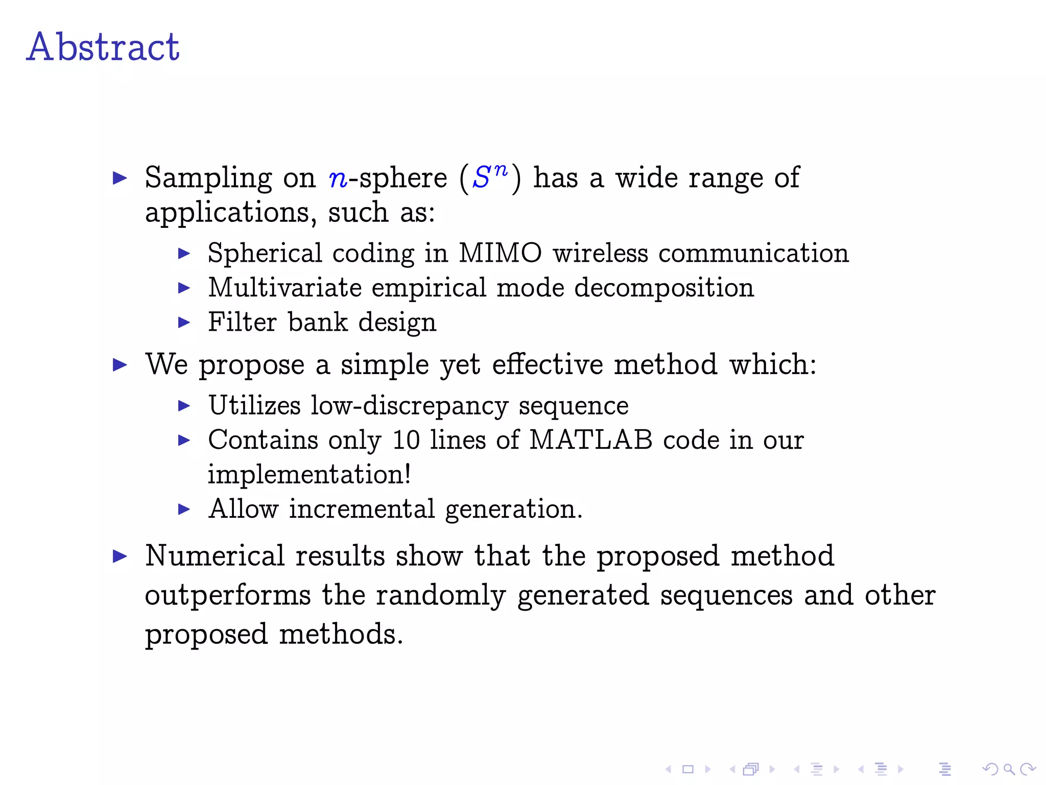
Abstract
Motivation and Applications
Review of Low Discrepancy Sequence
Van der Corput sequence on [0; 1]
Halton sequence on [0; 1]
Halton sequence on [0; 1]n
Unit Circle S1
Unit Sphere S2
Sphere Sn and SO(3)
Our approach
Numerical Experiments
Conclusions](https://image.slidesharecdn.com/n-sphere-140406035844-phpapp01/75/Sampling-with-Halton-Points-on-n-Sphere-2-2048.jpg)
![Agenda
Abstract
Motivation and Applications
Review of Low Discrepancy Sequence
Van der Corput sequence on [0; 1]
Halton sequence on [0; 1]
Halton sequence on [0; 1]n
Unit Circle S1
Unit Sphere S2
Sphere Sn and SO(3)
Our approach
Numerical Experiments
Conclusions](https://image.slidesharecdn.com/n-sphere-140406035844-phpapp01/75/Sampling-with-Halton-Points-on-n-Sphere-3-2048.jpg)
![Agenda
Abstract
Motivation and Applications
Review of Low Discrepancy Sequence
Van der Corput sequence on [0; 1]
Halton sequence on [0; 1]
Halton sequence on [0; 1]n
Unit Circle S1
Unit Sphere S2
Sphere Sn and SO(3)
Our approach
Numerical Experiments
Conclusions](https://image.slidesharecdn.com/n-sphere-140406035844-phpapp01/75/Sampling-with-Halton-Points-on-n-Sphere-5-2048.jpg)
![Motivation
The topic has been well studied for sphere in 3D, i.e. n = 2
Yet it is still unknown how to generate for n > 2.
Potential applications (for n > 2):
Robotic Motion Planning (S3
and SO(3)) [YJLM10]
Spherical coding in MIMO wireless communication [UL06]:
Cookbook for Unitary matrices
A code word = a point in Sn
Multivariate empirical mode decomposition [RM10]
Filter bank design [M+
11]](https://image.slidesharecdn.com/n-sphere-140406035844-phpapp01/75/Sampling-with-Halton-Points-on-n-Sphere-7-2048.jpg)
![Halton Sequence on Sn
Halton sequence on S2 has been well studied [CF97] by
using cylindrical coordinates.
Yet it is still little known for Sn where n > 2.
Note: The generalization of cylindrical coordinates does
NOT work in higher dimensions.](https://image.slidesharecdn.com/n-sphere-140406035844-phpapp01/75/Sampling-with-Halton-Points-on-n-Sphere-8-2048.jpg)
![Agenda
Abstract
Motivation and Applications
Review of Low Discrepancy Sequence
Van der Corput sequence on [0; 1]
Halton sequence on [0; 1]
Halton sequence on [0; 1]n
Unit Circle S1
Unit Sphere S2
Sphere Sn and SO(3)
Our approach
Numerical Experiments
Conclusions](https://image.slidesharecdn.com/n-sphere-140406035844-phpapp01/75/Sampling-with-Halton-Points-on-n-Sphere-9-2048.jpg)
![Basic: Van der Corput sequence
Generate a low discrepancy sequence over [0; 1]
Denote vd(k; b) as a Van der Corput sequence of k points,
where b is the base of a prime number.
MATLAB source code is available at http:
//www.mathworks.com/matlabcentral/fileexchange/
15354-generate-a-van-der-corput-sequence
Example](https://image.slidesharecdn.com/n-sphere-140406035844-phpapp01/75/Sampling-with-Halton-Points-on-n-Sphere-10-2048.jpg)
![Basic: Van der Corput sequence
Generate a low discrepancy sequence over [0; 1]
Denote vd(k; b) as a Van der Corput sequence of k points,
where b is the base of a prime number.
MATLAB source code is available at http:
//www.mathworks.com/matlabcentral/fileexchange/
15354-generate-a-van-der-corput-sequence
Example](https://image.slidesharecdn.com/n-sphere-140406035844-phpapp01/75/Sampling-with-Halton-Points-on-n-Sphere-11-2048.jpg)
![Basic: Van der Corput sequence
Generate a low discrepancy sequence over [0; 1]
Denote vd(k; b) as a Van der Corput sequence of k points,
where b is the base of a prime number.
MATLAB source code is available at http:
//www.mathworks.com/matlabcentral/fileexchange/
15354-generate-a-van-der-corput-sequence
Example](https://image.slidesharecdn.com/n-sphere-140406035844-phpapp01/75/Sampling-with-Halton-Points-on-n-Sphere-12-2048.jpg)
![Basic: Van der Corput sequence
Generate a low discrepancy sequence over [0; 1]
Denote vd(k; b) as a Van der Corput sequence of k points,
where b is the base of a prime number.
MATLAB source code is available at http:
//www.mathworks.com/matlabcentral/fileexchange/
15354-generate-a-van-der-corput-sequence
Example](https://image.slidesharecdn.com/n-sphere-140406035844-phpapp01/75/Sampling-with-Halton-Points-on-n-Sphere-13-2048.jpg)
![Basic: Van der Corput sequence
Generate a low discrepancy sequence over [0; 1]
Denote vd(k; b) as a Van der Corput sequence of k points,
where b is the base of a prime number.
MATLAB source code is available at http:
//www.mathworks.com/matlabcentral/fileexchange/
15354-generate-a-van-der-corput-sequence
Example](https://image.slidesharecdn.com/n-sphere-140406035844-phpapp01/75/Sampling-with-Halton-Points-on-n-Sphere-14-2048.jpg)
![Basic: Van der Corput sequence
Generate a low discrepancy sequence over [0; 1]
Denote vd(k; b) as a Van der Corput sequence of k points,
where b is the base of a prime number.
MATLAB source code is available at http:
//www.mathworks.com/matlabcentral/fileexchange/
15354-generate-a-van-der-corput-sequence
Example](https://image.slidesharecdn.com/n-sphere-140406035844-phpapp01/75/Sampling-with-Halton-Points-on-n-Sphere-15-2048.jpg)
![Basic: Van der Corput sequence
Generate a low discrepancy sequence over [0; 1]
Denote vd(k; b) as a Van der Corput sequence of k points,
where b is the base of a prime number.
MATLAB source code is available at http:
//www.mathworks.com/matlabcentral/fileexchange/
15354-generate-a-van-der-corput-sequence
Example](https://image.slidesharecdn.com/n-sphere-140406035844-phpapp01/75/Sampling-with-Halton-Points-on-n-Sphere-16-2048.jpg)
![Basic: Van der Corput sequence
Generate a low discrepancy sequence over [0; 1]
Denote vd(k; b) as a Van der Corput sequence of k points,
where b is the base of a prime number.
MATLAB source code is available at http:
//www.mathworks.com/matlabcentral/fileexchange/
15354-generate-a-van-der-corput-sequence
Example](https://image.slidesharecdn.com/n-sphere-140406035844-phpapp01/75/Sampling-with-Halton-Points-on-n-Sphere-17-2048.jpg)
![Basic: Van der Corput sequence
Generate a low discrepancy sequence over [0; 1]
Denote vd(k; b) as a Van der Corput sequence of k points,
where b is the base of a prime number.
MATLAB source code is available at http:
//www.mathworks.com/matlabcentral/fileexchange/
15354-generate-a-van-der-corput-sequence
Example](https://image.slidesharecdn.com/n-sphere-140406035844-phpapp01/75/Sampling-with-Halton-Points-on-n-Sphere-18-2048.jpg)
![Basic: Van der Corput sequence
Generate a low discrepancy sequence over [0; 1]
Denote vd(k; b) as a Van der Corput sequence of k points,
where b is the base of a prime number.
MATLAB source code is available at http:
//www.mathworks.com/matlabcentral/fileexchange/
15354-generate-a-van-der-corput-sequence
Example](https://image.slidesharecdn.com/n-sphere-140406035844-phpapp01/75/Sampling-with-Halton-Points-on-n-Sphere-19-2048.jpg)
![Basic: Van der Corput sequence
Generate a low discrepancy sequence over [0; 1]
Denote vd(k; b) as a Van der Corput sequence of k points,
where b is the base of a prime number.
MATLAB source code is available at http:
//www.mathworks.com/matlabcentral/fileexchange/
15354-generate-a-van-der-corput-sequence
Example](https://image.slidesharecdn.com/n-sphere-140406035844-phpapp01/75/Sampling-with-Halton-Points-on-n-Sphere-20-2048.jpg)
![Basic: Van der Corput sequence
Generate a low discrepancy sequence over [0; 1]
Denote vd(k; b) as a Van der Corput sequence of k points,
where b is the base of a prime number.
MATLAB source code is available at http:
//www.mathworks.com/matlabcentral/fileexchange/
15354-generate-a-van-der-corput-sequence
Example](https://image.slidesharecdn.com/n-sphere-140406035844-phpapp01/75/Sampling-with-Halton-Points-on-n-Sphere-21-2048.jpg)
![Basic: Van der Corput sequence
Generate a low discrepancy sequence over [0; 1]
Denote vd(k; b) as a Van der Corput sequence of k points,
where b is the base of a prime number.
MATLAB source code is available at http:
//www.mathworks.com/matlabcentral/fileexchange/
15354-generate-a-van-der-corput-sequence
Example](https://image.slidesharecdn.com/n-sphere-140406035844-phpapp01/75/Sampling-with-Halton-Points-on-n-Sphere-22-2048.jpg)
![Basic: Van der Corput sequence
Generate a low discrepancy sequence over [0; 1]
Denote vd(k; b) as a Van der Corput sequence of k points,
where b is the base of a prime number.
MATLAB source code is available at http:
//www.mathworks.com/matlabcentral/fileexchange/
15354-generate-a-van-der-corput-sequence
Example](https://image.slidesharecdn.com/n-sphere-140406035844-phpapp01/75/Sampling-with-Halton-Points-on-n-Sphere-23-2048.jpg)
![Basic: Van der Corput sequence
Generate a low discrepancy sequence over [0; 1]
Denote vd(k; b) as a Van der Corput sequence of k points,
where b is the base of a prime number.
MATLAB source code is available at http:
//www.mathworks.com/matlabcentral/fileexchange/
15354-generate-a-van-der-corput-sequence
Example](https://image.slidesharecdn.com/n-sphere-140406035844-phpapp01/75/Sampling-with-Halton-Points-on-n-Sphere-24-2048.jpg)
![Basic: Van der Corput sequence
Generate a low discrepancy sequence over [0; 1]
Denote vd(k; b) as a Van der Corput sequence of k points,
where b is the base of a prime number.
MATLAB source code is available at http:
//www.mathworks.com/matlabcentral/fileexchange/
15354-generate-a-van-der-corput-sequence
Example](https://image.slidesharecdn.com/n-sphere-140406035844-phpapp01/75/Sampling-with-Halton-Points-on-n-Sphere-25-2048.jpg)
![Unit Square [0; 1] ¢[0; 1]
Halton sequence: using 2
Van der Corput sequences
with different bases.
Example
[x; y] = [vd(k; 2); vd(k; 3)]](https://image.slidesharecdn.com/n-sphere-140406035844-phpapp01/75/Sampling-with-Halton-Points-on-n-Sphere-26-2048.jpg)
![Unit Square [0; 1] ¢[0; 1]
Halton sequence: using 2
Van der Corput sequences
with different bases.
Example
[x; y] = [vd(k; 2); vd(k; 3)]](https://image.slidesharecdn.com/n-sphere-140406035844-phpapp01/75/Sampling-with-Halton-Points-on-n-Sphere-27-2048.jpg)
![Unit Square [0; 1] ¢[0; 1]
Halton sequence: using 2
Van der Corput sequences
with different bases.
Example
[x; y] = [vd(k; 2); vd(k; 3)]](https://image.slidesharecdn.com/n-sphere-140406035844-phpapp01/75/Sampling-with-Halton-Points-on-n-Sphere-28-2048.jpg)
![Unit Square [0; 1] ¢[0; 1]
Halton sequence: using 2
Van der Corput sequences
with different bases.
Example
[x; y] = [vd(k; 2); vd(k; 3)]](https://image.slidesharecdn.com/n-sphere-140406035844-phpapp01/75/Sampling-with-Halton-Points-on-n-Sphere-29-2048.jpg)
![Unit Square [0; 1] ¢[0; 1]
Halton sequence: using 2
Van der Corput sequences
with different bases.
Example
[x; y] = [vd(k; 2); vd(k; 3)]](https://image.slidesharecdn.com/n-sphere-140406035844-phpapp01/75/Sampling-with-Halton-Points-on-n-Sphere-30-2048.jpg)
![Unit Square [0; 1] ¢[0; 1]
Halton sequence: using 2
Van der Corput sequences
with different bases.
Example
[x; y] = [vd(k; 2); vd(k; 3)]](https://image.slidesharecdn.com/n-sphere-140406035844-phpapp01/75/Sampling-with-Halton-Points-on-n-Sphere-31-2048.jpg)
![Unit Square [0; 1] ¢[0; 1]
Halton sequence: using 2
Van der Corput sequences
with different bases.
Example
[x; y] = [vd(k; 2); vd(k; 3)]](https://image.slidesharecdn.com/n-sphere-140406035844-phpapp01/75/Sampling-with-Halton-Points-on-n-Sphere-32-2048.jpg)
![Unit Square [0; 1] ¢[0; 1]
Halton sequence: using 2
Van der Corput sequences
with different bases.
Example
[x; y] = [vd(k; 2); vd(k; 3)]](https://image.slidesharecdn.com/n-sphere-140406035844-phpapp01/75/Sampling-with-Halton-Points-on-n-Sphere-33-2048.jpg)
![Unit Square [0; 1] ¢[0; 1]
Halton sequence: using 2
Van der Corput sequences
with different bases.
Example
[x; y] = [vd(k; 2); vd(k; 3)]](https://image.slidesharecdn.com/n-sphere-140406035844-phpapp01/75/Sampling-with-Halton-Points-on-n-Sphere-34-2048.jpg)
![Unit Square [0; 1] ¢[0; 1]
Halton sequence: using 2
Van der Corput sequences
with different bases.
Example
[x; y] = [vd(k; 2); vd(k; 3)]](https://image.slidesharecdn.com/n-sphere-140406035844-phpapp01/75/Sampling-with-Halton-Points-on-n-Sphere-35-2048.jpg)
![Unit Square [0; 1] ¢[0; 1]
Halton sequence: using 2
Van der Corput sequences
with different bases.
Example
[x; y] = [vd(k; 2); vd(k; 3)]](https://image.slidesharecdn.com/n-sphere-140406035844-phpapp01/75/Sampling-with-Halton-Points-on-n-Sphere-36-2048.jpg)
![Unit Square [0; 1] ¢[0; 1]
Halton sequence: using 2
Van der Corput sequences
with different bases.
Example
[x; y] = [vd(k; 2); vd(k; 3)]](https://image.slidesharecdn.com/n-sphere-140406035844-phpapp01/75/Sampling-with-Halton-Points-on-n-Sphere-37-2048.jpg)
![Unit Square [0; 1] ¢[0; 1]
Halton sequence: using 2
Van der Corput sequences
with different bases.
Example
[x; y] = [vd(k; 2); vd(k; 3)]](https://image.slidesharecdn.com/n-sphere-140406035844-phpapp01/75/Sampling-with-Halton-Points-on-n-Sphere-38-2048.jpg)
![Unit Square [0; 1] ¢[0; 1]
Halton sequence: using 2
Van der Corput sequences
with different bases.
Example
[x; y] = [vd(k; 2); vd(k; 3)]](https://image.slidesharecdn.com/n-sphere-140406035844-phpapp01/75/Sampling-with-Halton-Points-on-n-Sphere-39-2048.jpg)
![Unit Square [0; 1] ¢[0; 1]
Halton sequence: using 2
Van der Corput sequences
with different bases.
Example
[x; y] = [vd(k; 2); vd(k; 3)]](https://image.slidesharecdn.com/n-sphere-140406035844-phpapp01/75/Sampling-with-Halton-Points-on-n-Sphere-40-2048.jpg)
![Unit Square [0; 1] ¢[0; 1]
Halton sequence: using 2
Van der Corput sequences
with different bases.
Example
[x; y] = [vd(k; 2); vd(k; 3)]](https://image.slidesharecdn.com/n-sphere-140406035844-phpapp01/75/Sampling-with-Halton-Points-on-n-Sphere-41-2048.jpg)
![Unit Square [0; 1] ¢[0; 1]
Halton sequence: using 2
Van der Corput sequences
with different bases.
Example
[x; y] = [vd(k; 2); vd(k; 3)]](https://image.slidesharecdn.com/n-sphere-140406035844-phpapp01/75/Sampling-with-Halton-Points-on-n-Sphere-42-2048.jpg)
![Unit Square [0; 1] ¢[0; 1]
Halton sequence: using 2
Van der Corput sequences
with different bases.
Example
[x; y] = [vd(k; 2); vd(k; 3)]](https://image.slidesharecdn.com/n-sphere-140406035844-phpapp01/75/Sampling-with-Halton-Points-on-n-Sphere-43-2048.jpg)
![Unit Square [0; 1] ¢[0; 1]
Halton sequence: using 2
Van der Corput sequences
with different bases.
Example
[x; y] = [vd(k; 2); vd(k; 3)]](https://image.slidesharecdn.com/n-sphere-140406035844-phpapp01/75/Sampling-with-Halton-Points-on-n-Sphere-44-2048.jpg)
![Unit Square [0; 1] ¢[0; 1]
Halton sequence: using 2
Van der Corput sequences
with different bases.
Example
[x; y] = [vd(k; 2); vd(k; 3)]](https://image.slidesharecdn.com/n-sphere-140406035844-phpapp01/75/Sampling-with-Halton-Points-on-n-Sphere-45-2048.jpg)
![Unit Square [0; 1] ¢[0; 1]
Halton sequence: using 2
Van der Corput sequences
with different bases.
Example
[x; y] = [vd(k; 2); vd(k; 3)]](https://image.slidesharecdn.com/n-sphere-140406035844-phpapp01/75/Sampling-with-Halton-Points-on-n-Sphere-46-2048.jpg)
![Unit Square [0; 1] ¢[0; 1]
Halton sequence: using 2
Van der Corput sequences
with different bases.
Example
[x; y] = [vd(k; 2); vd(k; 3)]](https://image.slidesharecdn.com/n-sphere-140406035844-phpapp01/75/Sampling-with-Halton-Points-on-n-Sphere-47-2048.jpg)
![Unit Square [0; 1] ¢[0; 1]
Halton sequence: using 2
Van der Corput sequences
with different bases.
Example
[x; y] = [vd(k; 2); vd(k; 3)]](https://image.slidesharecdn.com/n-sphere-140406035844-phpapp01/75/Sampling-with-Halton-Points-on-n-Sphere-48-2048.jpg)
![Unit Square [0; 1] ¢[0; 1]
Halton sequence: using 2
Van der Corput sequences
with different bases.
Example
[x; y] = [vd(k; 2); vd(k; 3)]](https://image.slidesharecdn.com/n-sphere-140406035844-phpapp01/75/Sampling-with-Halton-Points-on-n-Sphere-49-2048.jpg)
![Unit Square [0; 1] ¢[0; 1]
Halton sequence: using 2
Van der Corput sequences
with different bases.
Example
[x; y] = [vd(k; 2); vd(k; 3)]](https://image.slidesharecdn.com/n-sphere-140406035844-phpapp01/75/Sampling-with-Halton-Points-on-n-Sphere-50-2048.jpg)
![Unit Hypercube [0; 1]
n
Generally we can generate Halton sequence in a unit
hypercube [0; 1]n :
[x1; x2; : : : ; xn ] = [vd(k; b1); vd(k; b2); : : : ; vd(k; bn )]
A wide range of applications on Quasi-Monte Carlo
Methods (QMC).](https://image.slidesharecdn.com/n-sphere-140406035844-phpapp01/75/Sampling-with-Halton-Points-on-n-Sphere-51-2048.jpg)
![Unit Circle S1
Can be generated by mapping the
Van der Corput sequence to [0; 2]
= 2 ¡vd(k; b)
[x; y] = [cos ; sin ]](https://image.slidesharecdn.com/n-sphere-140406035844-phpapp01/75/Sampling-with-Halton-Points-on-n-Sphere-52-2048.jpg)
![Unit Circle S1
Can be generated by mapping the
Van der Corput sequence to [0; 2]
= 2 ¡vd(k; b)
[x; y] = [cos ; sin ]](https://image.slidesharecdn.com/n-sphere-140406035844-phpapp01/75/Sampling-with-Halton-Points-on-n-Sphere-53-2048.jpg)
![Unit Circle S1
Can be generated by mapping the
Van der Corput sequence to [0; 2]
= 2 ¡vd(k; b)
[x; y] = [cos ; sin ]](https://image.slidesharecdn.com/n-sphere-140406035844-phpapp01/75/Sampling-with-Halton-Points-on-n-Sphere-54-2048.jpg)
![Unit Circle S1
Can be generated by mapping the
Van der Corput sequence to [0; 2]
= 2 ¡vd(k; b)
[x; y] = [cos ; sin ]](https://image.slidesharecdn.com/n-sphere-140406035844-phpapp01/75/Sampling-with-Halton-Points-on-n-Sphere-55-2048.jpg)
![Unit Circle S1
Can be generated by mapping the
Van der Corput sequence to [0; 2]
= 2 ¡vd(k; b)
[x; y] = [cos ; sin ]](https://image.slidesharecdn.com/n-sphere-140406035844-phpapp01/75/Sampling-with-Halton-Points-on-n-Sphere-56-2048.jpg)
![Unit Circle S1
Can be generated by mapping the
Van der Corput sequence to [0; 2]
= 2 ¡vd(k; b)
[x; y] = [cos ; sin ]](https://image.slidesharecdn.com/n-sphere-140406035844-phpapp01/75/Sampling-with-Halton-Points-on-n-Sphere-57-2048.jpg)
![Unit Circle S1
Can be generated by mapping the
Van der Corput sequence to [0; 2]
= 2 ¡vd(k; b)
[x; y] = [cos ; sin ]](https://image.slidesharecdn.com/n-sphere-140406035844-phpapp01/75/Sampling-with-Halton-Points-on-n-Sphere-58-2048.jpg)
![Unit Circle S1
Can be generated by mapping the
Van der Corput sequence to [0; 2]
= 2 ¡vd(k; b)
[x; y] = [cos ; sin ]](https://image.slidesharecdn.com/n-sphere-140406035844-phpapp01/75/Sampling-with-Halton-Points-on-n-Sphere-59-2048.jpg)
![Unit Circle S1
Can be generated by mapping the
Van der Corput sequence to [0; 2]
= 2 ¡vd(k; b)
[x; y] = [cos ; sin ]](https://image.slidesharecdn.com/n-sphere-140406035844-phpapp01/75/Sampling-with-Halton-Points-on-n-Sphere-60-2048.jpg)
![Unit Circle S1
Can be generated by mapping the
Van der Corput sequence to [0; 2]
= 2 ¡vd(k; b)
[x; y] = [cos ; sin ]](https://image.slidesharecdn.com/n-sphere-140406035844-phpapp01/75/Sampling-with-Halton-Points-on-n-Sphere-61-2048.jpg)
![Unit Circle S1
Can be generated by mapping the
Van der Corput sequence to [0; 2]
= 2 ¡vd(k; b)
[x; y] = [cos ; sin ]](https://image.slidesharecdn.com/n-sphere-140406035844-phpapp01/75/Sampling-with-Halton-Points-on-n-Sphere-62-2048.jpg)
![Unit Circle S1
Can be generated by mapping the
Van der Corput sequence to [0; 2]
= 2 ¡vd(k; b)
[x; y] = [cos ; sin ]](https://image.slidesharecdn.com/n-sphere-140406035844-phpapp01/75/Sampling-with-Halton-Points-on-n-Sphere-63-2048.jpg)
![Unit Circle S1
Can be generated by mapping the
Van der Corput sequence to [0; 2]
= 2 ¡vd(k; b)
[x; y] = [cos ; sin ]](https://image.slidesharecdn.com/n-sphere-140406035844-phpapp01/75/Sampling-with-Halton-Points-on-n-Sphere-64-2048.jpg)
![Unit Circle S1
Can be generated by mapping the
Van der Corput sequence to [0; 2]
= 2 ¡vd(k; b)
[x; y] = [cos ; sin ]](https://image.slidesharecdn.com/n-sphere-140406035844-phpapp01/75/Sampling-with-Halton-Points-on-n-Sphere-65-2048.jpg)
![Unit Circle S1
Can be generated by mapping the
Van der Corput sequence to [0; 2]
= 2 ¡vd(k; b)
[x; y] = [cos ; sin ]](https://image.slidesharecdn.com/n-sphere-140406035844-phpapp01/75/Sampling-with-Halton-Points-on-n-Sphere-66-2048.jpg)
![Unit Circle S1
Can be generated by mapping the
Van der Corput sequence to [0; 2]
= 2 ¡vd(k; b)
[x; y] = [cos ; sin ]](https://image.slidesharecdn.com/n-sphere-140406035844-phpapp01/75/Sampling-with-Halton-Points-on-n-Sphere-67-2048.jpg)
![Unit Circle S1
Can be generated by mapping the
Van der Corput sequence to [0; 2]
= 2 ¡vd(k; b)
[x; y] = [cos ; sin ]](https://image.slidesharecdn.com/n-sphere-140406035844-phpapp01/75/Sampling-with-Halton-Points-on-n-Sphere-68-2048.jpg)
![Unit Sphere S2
Has been applied for computer
graphic applications [WLH97]
[z; x; y]
= [cos ; sin cos '; sin sin ']
= [z;
p
1 z2 cos ';
p
1 z2 sin ']
' = 2 ¡vd(k; b1) % map to
[0; 2]
z = 2 ¡vd(k; b2) 1 % map to
[ 1; 1]](https://image.slidesharecdn.com/n-sphere-140406035844-phpapp01/75/Sampling-with-Halton-Points-on-n-Sphere-69-2048.jpg)
![Sphere S3
and SO(3)
Deterministic point sets
Optimal grid point sets for S3
, SO(3) [Lubotzky, Phillips,
Sarnak 86] [Mitchell 07]
No Halton sequences so far to the best of our knowledge](https://image.slidesharecdn.com/n-sphere-140406035844-phpapp01/75/Sampling-with-Halton-Points-on-n-Sphere-70-2048.jpg)
![Agenda
Abstract
Motivation and Applications
Review of Low Discrepancy Sequence
Van der Corput sequence on [0; 1]
Halton sequence on [0; 1]
Halton sequence on [0; 1]n
Unit Circle S1
Unit Sphere S2
Sphere Sn and SO(3)
Our approach
Numerical Experiments
Conclusions](https://image.slidesharecdn.com/n-sphere-140406035844-phpapp01/75/Sampling-with-Halton-Points-on-n-Sphere-71-2048.jpg)
![SO(3) or S3
Hopf Coordinates
Hopf coordinates (cf. [YJLM10])
x1 = cos(=2) cos( =2)
x2 = cos(=2) sin( =2)
x3 = sin(=2) cos(' + =2)
x4 = sin(=2) sin(' + =2)
S3 is a principal circle bundle
over the S2](https://image.slidesharecdn.com/n-sphere-140406035844-phpapp01/75/Sampling-with-Halton-Points-on-n-Sphere-72-2048.jpg)
![Hopf Coordinates for SO(3) or S3
Similar to the Halton sequence generation on S2, we perform
the mapping:
' = 2 ¡vd(k; b1) % map to [0; 2]
= 2 ¡vd(k; b2) % map to [0; 2] for SO(3), or
= 4 ¡vd(k; b2) % map to [0; 4] for S3
z = 2 ¡vd(k; b3) 1 % map to [ 1; 1]
= cos 1 z](https://image.slidesharecdn.com/n-sphere-140406035844-phpapp01/75/Sampling-with-Halton-Points-on-n-Sphere-73-2048.jpg)
![10 Lines of MATLAB Code
1 function[s] = sphere3_hopf (k,b)
2 % sphere3_hopf Halton sequence
3 varphi = 2*pi*vdcorput(k,b(1)); % map to [0, 2*pi]
4 psi = 4*pi*vdcorput(k,b(2)); % map to [0, 4*pi]
5 z = 2* vdcorput(k,b(3)) - 1; % map to [-1, 1]
6 theta = acos(z);
7 cos_eta = cos(theta /2);
8 sin_eta = sin(theta /2);
9 s = [cos_eta .* cos(psi /2), ...
10 cos_eta .* sin(psi /2), ...
11 sin_eta .* cos(varphi + psi /2), ...
12 sin_eta .* sin(varphi + psi /2)];](https://image.slidesharecdn.com/n-sphere-140406035844-phpapp01/75/Sampling-with-Halton-Points-on-n-Sphere-74-2048.jpg)
![How to Generate the Point Set
p0 = [cos 1; sin 1] where 1 = 2 ¡vd(k; b1)
Let fj () =
R
sinj
d, where P (0; ).
Note: fj () is a monotonic increasing function in (0; )
Map vd(k; bj ) uniformly to fj ():
tj = fj (0) + (fj () fj (0))vd(k; bj )
Let j = f 1
j (tj )
Define pn recursively as:
pn = [cos n ; sin n ¡pn 1]](https://image.slidesharecdn.com/n-sphere-140406035844-phpapp01/75/Sampling-with-Halton-Points-on-n-Sphere-77-2048.jpg)
![Agenda
Abstract
Motivation and Applications
Review of Low Discrepancy Sequence
Van der Corput sequence on [0; 1]
Halton sequence on [0; 1]
Halton sequence on [0; 1]n
Unit Circle S1
Unit Sphere S2
Sphere Sn and SO(3)
Our approach
Numerical Experiments
Conclusions](https://image.slidesharecdn.com/n-sphere-140406035844-phpapp01/75/Sampling-with-Halton-Points-on-n-Sphere-79-2048.jpg)
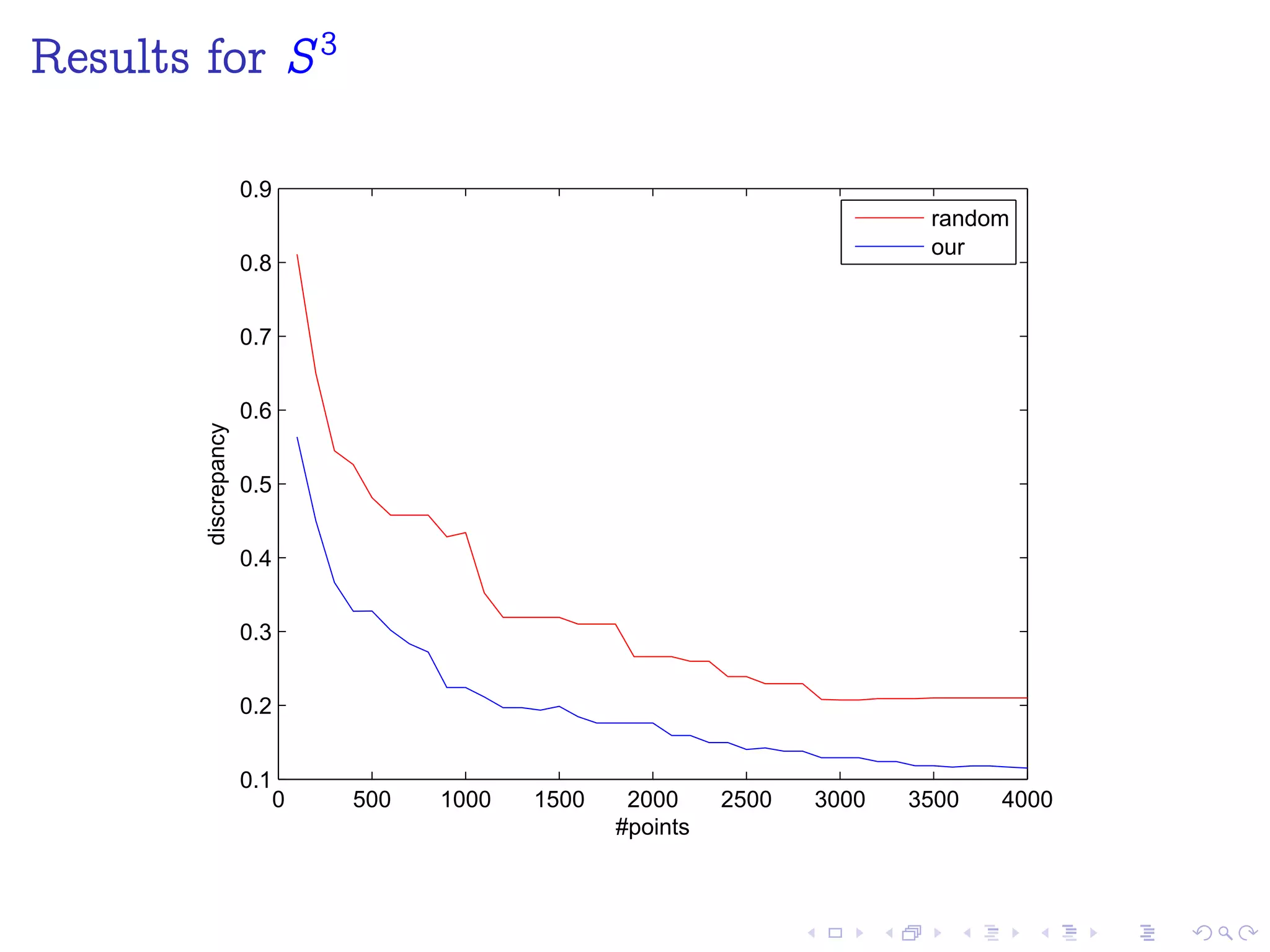
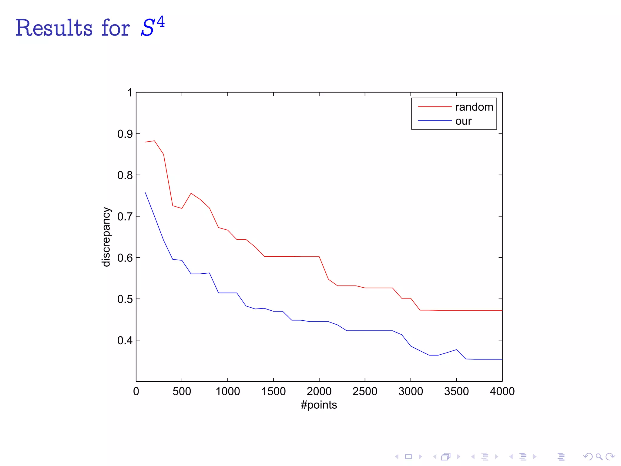
![Random sequences
To generate random points on Sn , spherical symmetry of
the multidimensional Gaussian density function can be
exploited.
Then the normalized vector (xi =kxi k) is uniformly
distributed over the hypersphere Sn . [Fishman, G. F.
(1996)]](https://image.slidesharecdn.com/n-sphere-140406035844-phpapp01/75/Sampling-with-Halton-Points-on-n-Sphere-81-2048.jpg)
![Agenda
Abstract
Motivation and Applications
Review of Low Discrepancy Sequence
Van der Corput sequence on [0; 1]
Halton sequence on [0; 1]
Halton sequence on [0; 1]n
Unit Circle S1
Unit Sphere S2
Sphere Sn and SO(3)
Our approach
Numerical Experiments
Conclusions](https://image.slidesharecdn.com/n-sphere-140406035844-phpapp01/75/Sampling-with-Halton-Points-on-n-Sphere-85-2048.jpg)
![References I
[CF97] Jianjun Cui and Willi Freeden, Equidistribution on the sphere, SIAM
Journal on Scientific Computing 18 (1997), no. 2, 595–609.
[M+11] DP Mandic et al., Filter bank property of multivariate empirical mode
decomposition, Signal Processing, IEEE Transactions on 59 (2011),
no. 5, 2421–2426.
[RM10] Naveed Rehman and Danilo P Mandic, Multivariate empirical mode
decomposition, Proceedings of the Royal Society A: Mathematical,
Physical and Engineering Science 466 (2010), no. 2117, 1291–1302.
[UL06] Zoran Utkovski and Juergen Lindner, On the construction of
non-coherent space time codes from high-dimensional spherical codes,
Spread Spectrum Techniques and Applications, 2006 IEEE Ninth
International Symposium on, IEEE, 2006, pp. 327–331.
[WLH97] Tien-Tsin Wong, Wai-Shing Luk, and Pheng-Ann Heng, Sampling with
hammersley and halton points, Journal of graphics tools 2 (1997),
no. 2, 9–24.
[YJLM10] Anna Yershova, Swati Jain, Steven M LaValle, and Julie C Mitchell,
Generating uniform incremental grids on so (3) using the hopf
fibration, The International journal of robotics research 29 (2010),
no. 7, 801–812.](https://image.slidesharecdn.com/n-sphere-140406035844-phpapp01/75/Sampling-with-Halton-Points-on-n-Sphere-87-2048.jpg)

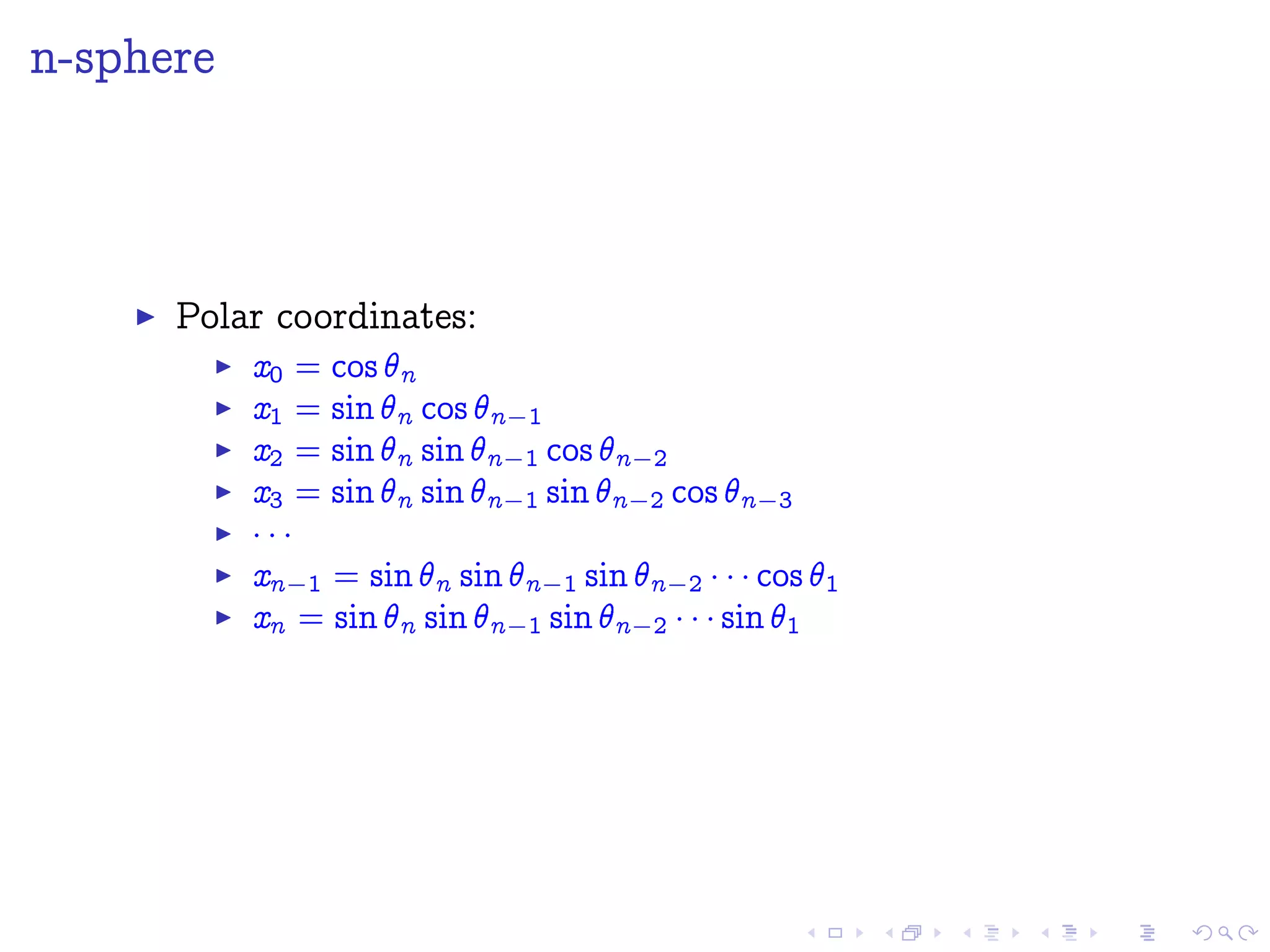
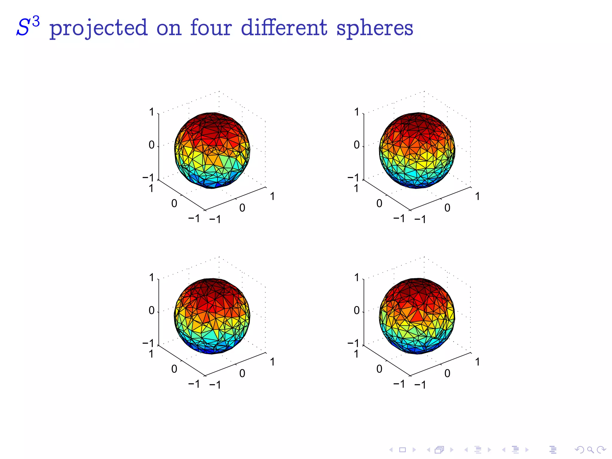
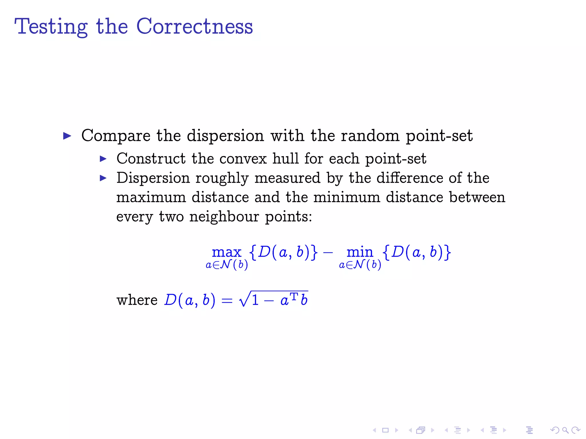
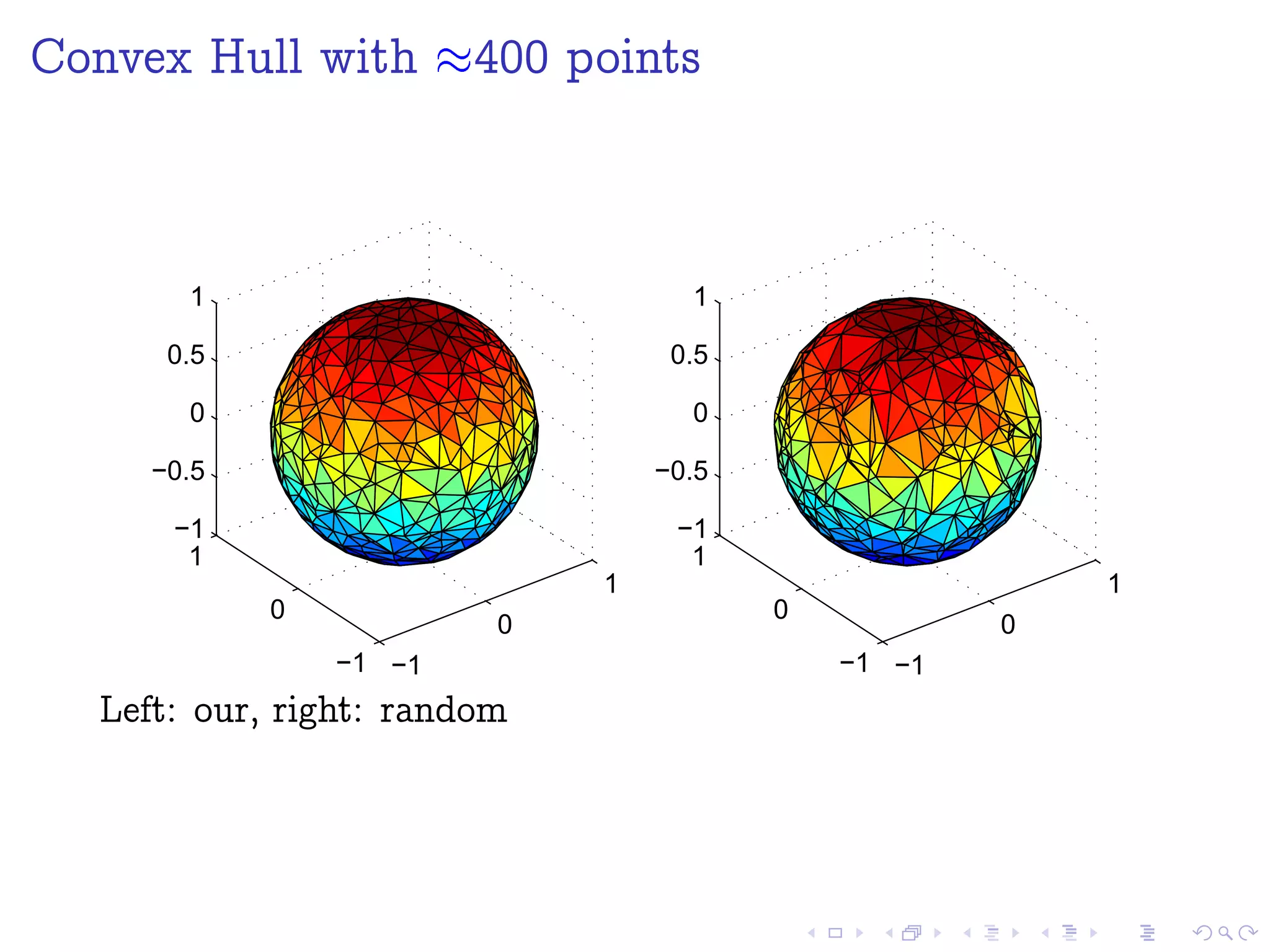
The document discusses sampling points on an n-sphere (Sn) using low-discrepancy sequences. It reviews Van der Corput and Halton sequences, which generate low-discrepancy samples on the unit interval [0,1]. The document proposes using Halton points, which extend the Halton sequence to higher dimensions, to sample points on Sn. Numerical experiments show this method outperforms random sampling and other proposed methods.


![Coded Agents – with UiPath SDK + LangGraph [Virtual Hands-on Workshop]](https://cdn.slidesharecdn.com/ss_thumbnails/codedagentsdeck-251215155422-5497c599-thumbnail.jpg?width=640&height=640&fit=bounds)


