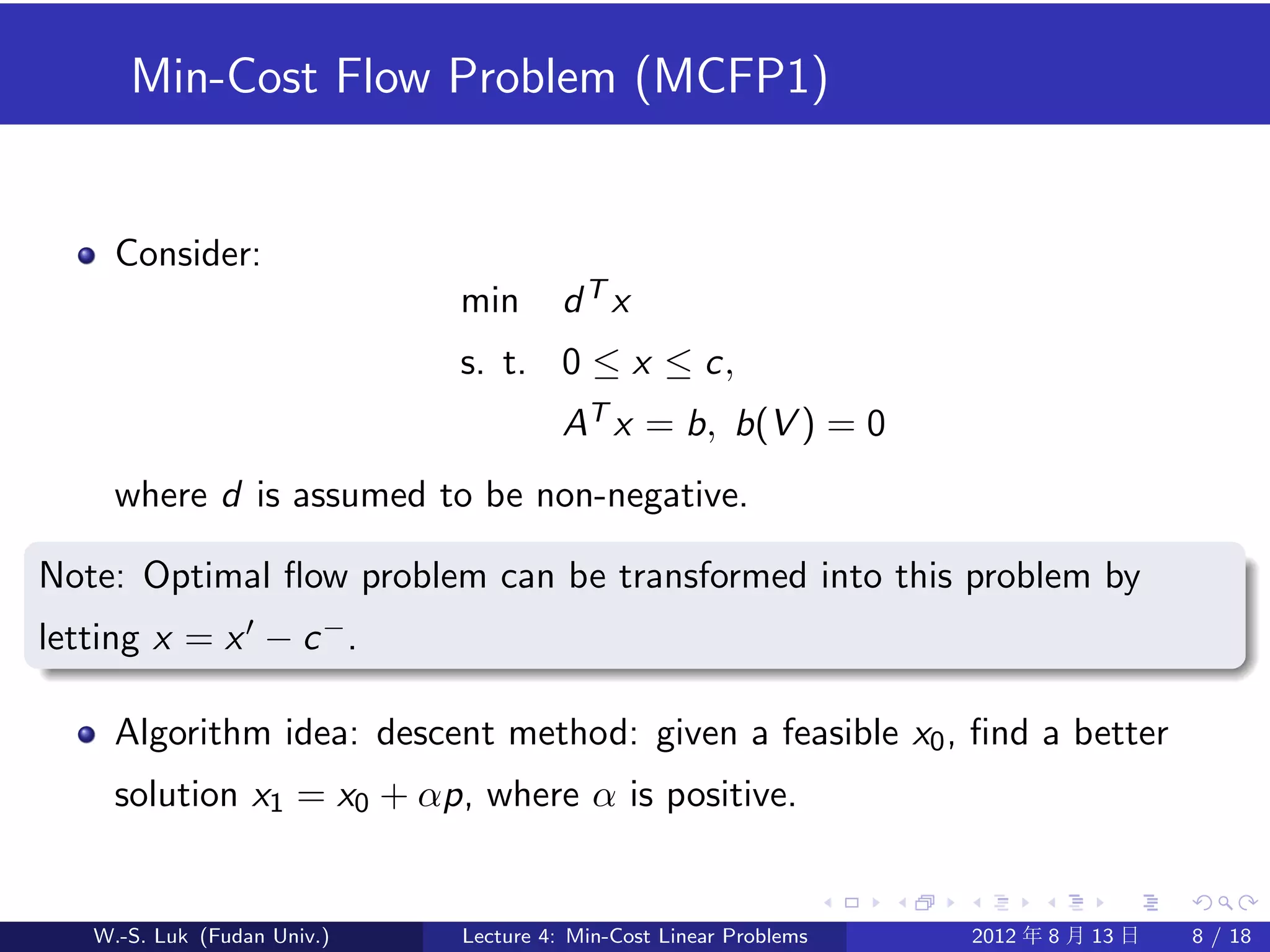
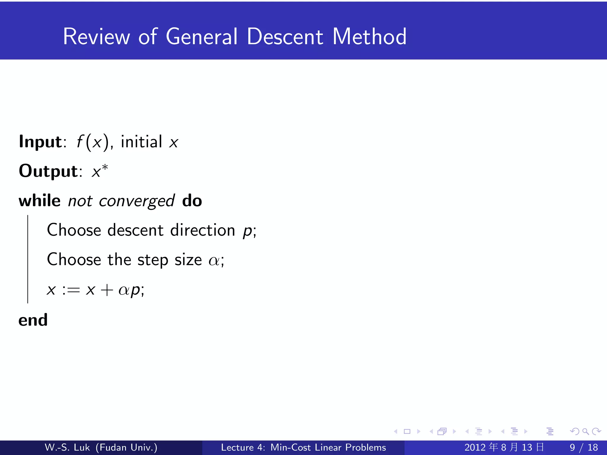
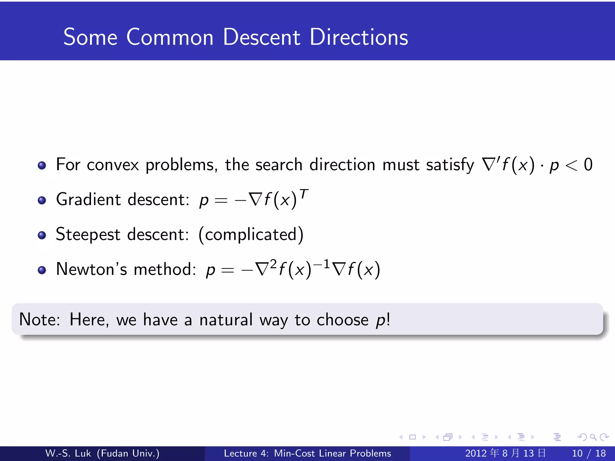
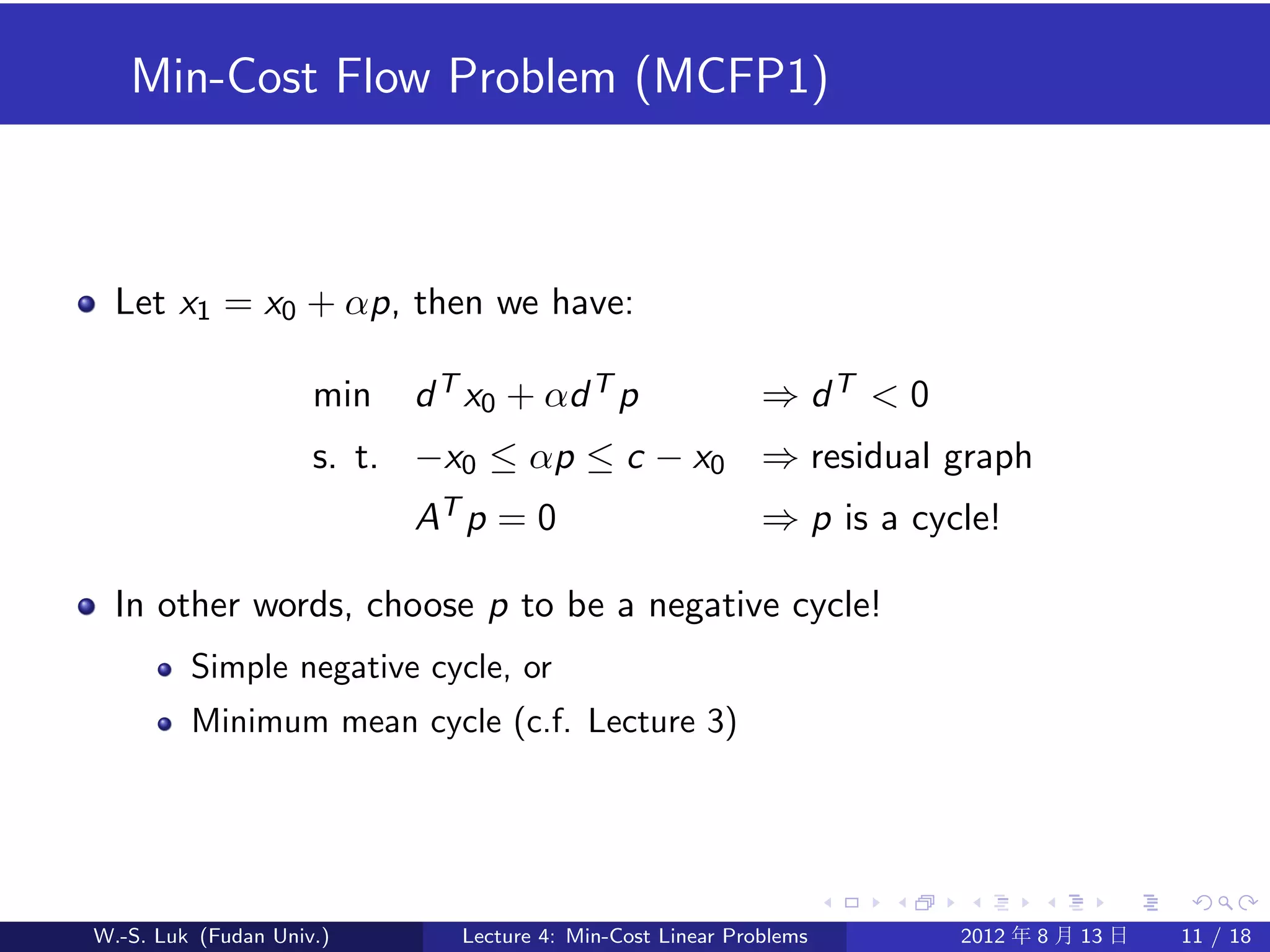
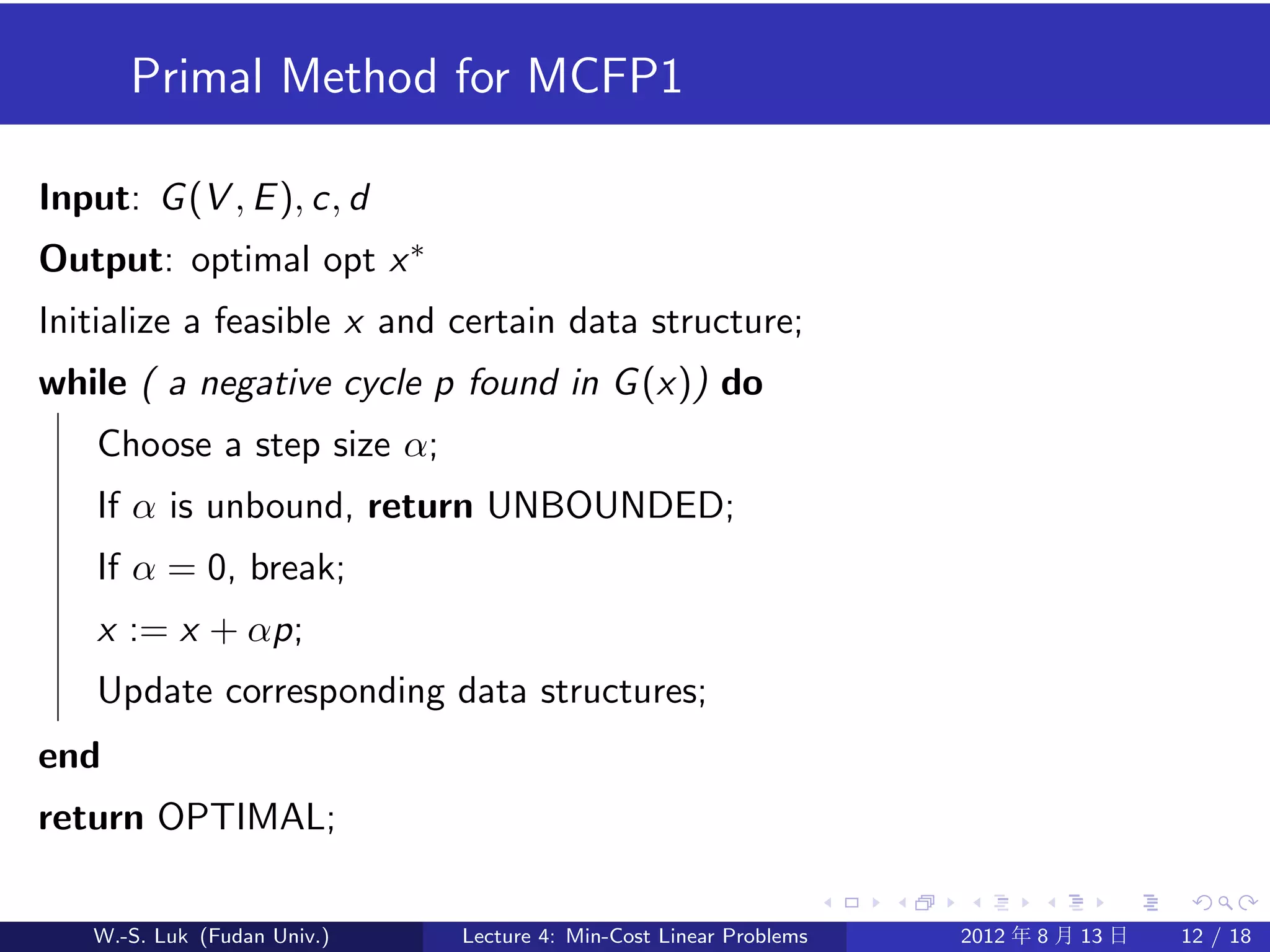
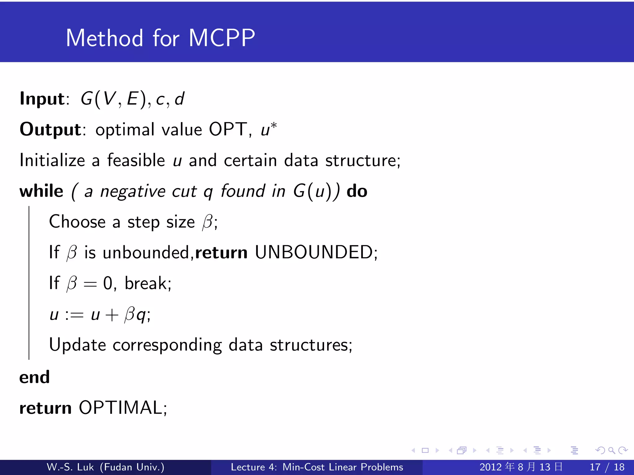
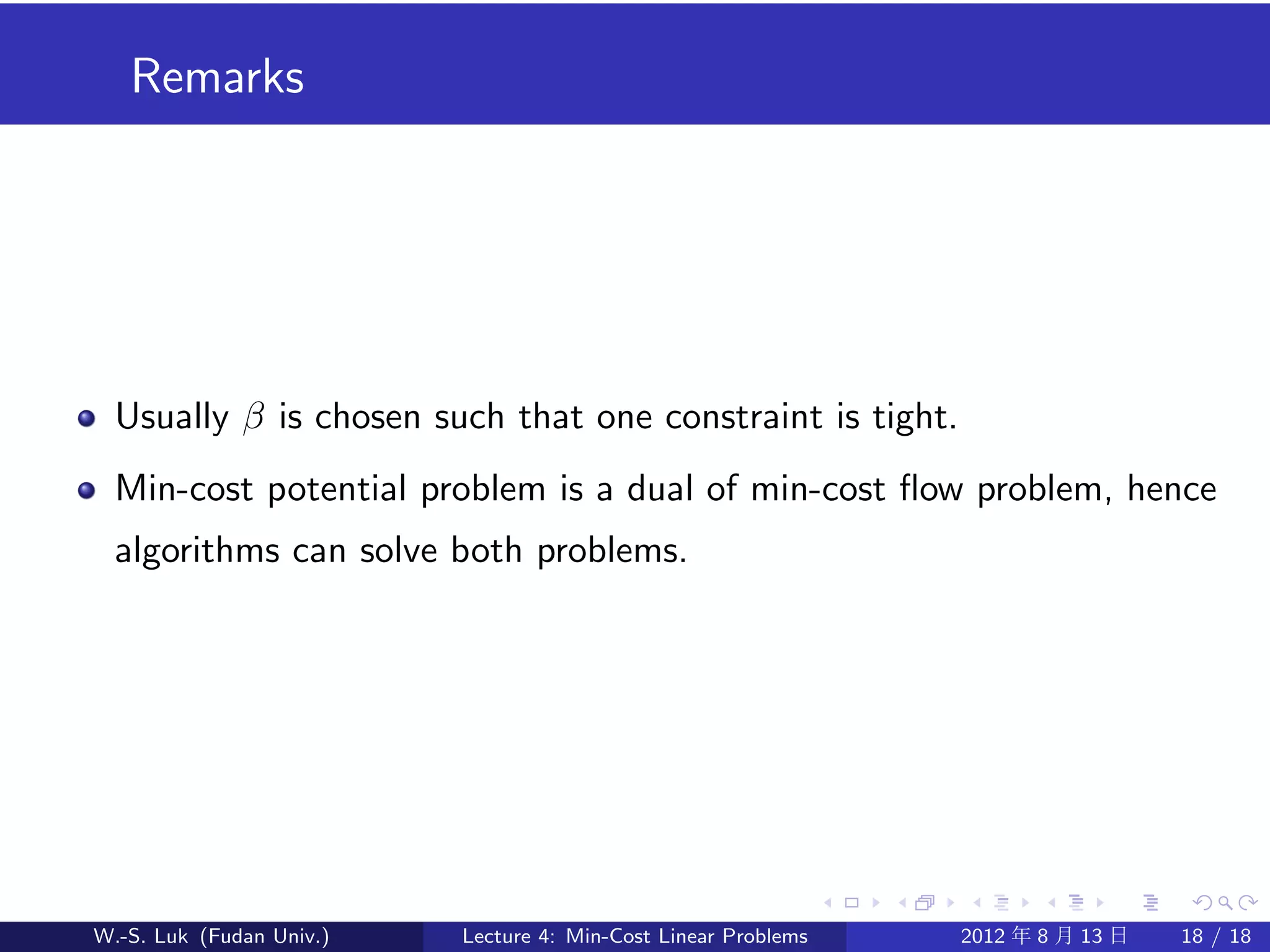
The document summarizes algorithms for solving min-cost linear problems, including min-cost flow problems and min-cost potential problems. It describes how these problems can be formulated and solved using descent methods, where the search direction is chosen as a negative cycle or cut with minimum cost. Iteratively, an optimal solution is found by moving in the direction of negative cycles or cuts and updating residual graphs and data structures. Duality between the min-cost flow and potential problems is also discussed.

1. Lecture 4: Min-Cost Linear Problems
Wai-Shing Luk (陆伟成)
Fudan University
2012 年 8 月 13 日
W.-S. Luk (Fudan Univ.) Lecture 4: Min-Cost Linear Problems 2012 年 8 月 13 日 1 / 18

2. Elementary Optimal Problems
Elementary Flow Problem: Elementary Potential Problem:
min dT x + p max b T u − (c T y + q)
s. t. c ≤ x, s. t. y ≤ d,
AT x = b, b(V ) = 0 Au = y
Theorem
The problems are dual to each other if
p + q = −c T d, (x − c)T (d − y ) = 0, c ≤ x, y ≤ d
Proof.
Since b T u = (AT x)T u = x T Au = x T y , [min] − [max] = (d T x + p) −
(b T u − [c T y + q]) = d T x + c T y − x T y + p + q = (x − c)T (d − y ) ≥ 0
[min] - [max] when equality holds.
W.-S. Luk (Fudan Univ.) Lecture 4: Min-Cost Linear Problems 2012 年 8 月 13 日 2 / 18

3. Remark 1
We can formulate a linear problem either in its primal form or in its
dual form, depending on which one is more appropriate, for example,
whether design variables are in integral domain:
max-flow problem (i.e. d T = [−1, −1, · · · , −1]T ) may be better to be
solved by a dual method.
W.-S. Luk (Fudan Univ.) Lecture 4: Min-Cost Linear Problems 2012 年 8 月 13 日 3 / 18

4. Linear Optimal Problems
Optimal Flow Problem: Optimal Potential Problem:
min dT x + p max b T u − (c T y + q)
s. t. c − ≤ x ≤ c + , s. t. d − ≤ y ≤ d + ,
AT x = b, b(V ) = 0 Au = y
By modifying the network:
This problem can be reduced to the elementary case [?, pp.275–276]
Piecewise linear convex cost can be reduced to this linear problem [?,
p.239,p.260]
The problem has been studied extensively with a lot of applications.
W.-S. Luk (Fudan Univ.) Lecture 4: Min-Cost Linear Problems 2012 年 8 月 13 日 4 / 18

5. Remark
We can transform the cost function to be non-negative by reversing
the orientation of the negative cost edges.
Then reduce the problem to the elementary case.
Most software packages only solve the problems in primal forms,
usually with c − = 0.
W.-S. Luk (Fudan Univ.) Lecture 4: Min-Cost Linear Problems 2012 年 8 月 13 日 5 / 18

6. Algorithms for Optimal Flow Problems
Successive shortest path algorithm
Cycle cancellation method
iteratively insert additional minimal flows according to a negative cycle
of the residual network, until no negative cycle is found.
W.-S. Luk (Fudan Univ.) Lecture 4: Min-Cost Linear Problems 2012 年 8 月 13 日 6 / 18

7. For Special Cases
Max flow problem (d = −[1, · · · , 1])
Ford-Fulkerson algorithm: iteratively insert additional minimal flows
according to an argument path of the residual network, until no
argument path of the residual network is found.
Preflow Push-Relabel algorithm (dual method???)
Matching problems ([c − , c + ] = [0, 1])
Edmond’s blossom algorithm
W.-S. Luk (Fudan Univ.) Lecture 4: Min-Cost Linear Problems 2012 年 8 月 13 日 7 / 18

8. Min-Cost Flow Problem (MCFP1)
Consider:
min dT x
s. t. 0 ≤ x ≤ c,
AT x = b, b(V ) = 0
where d is assumed to be non-negative.
Note: Optimal flow problem can be transformed into this problem by
letting x = x − c − .
Algorithm idea: descent method: given a feasible x0 , find a better
solution x1 = x0 + αp, where α is positive.
W.-S. Luk (Fudan Univ.) Lecture 4: Min-Cost Linear Problems 2012 年 8 月 13 日 8 / 18

9. Review of General Descent Method
Input: f (x), initial x
Output: x ∗
while not converged do
Choose descent direction p;
Choose the step size α;
x := x + αp;
end
W.-S. Luk (Fudan Univ.) Lecture 4: Min-Cost Linear Problems 2012 年 8 月 13 日 9 / 18

10. Some Common Descent Directions
For convex problems, the search direction must satisfy f (x) · p < 0
Gradient descent: p = − f (x)T
Steepest descent: (complicated)
Newton’s method: p = − 2 f (x)−1 f (x)
Note: Here, we have a natural way to choose p!
W.-S. Luk (Fudan Univ.) Lecture 4: Min-Cost Linear Problems 2012 年 8 月 13 日 10 / 18

11. Min-Cost Flow Problem (MCFP1)
Let x1 = x0 + αp, then we have:
min d T x0 + αd T p ⇒ dT < 0
s. t. −x0 ≤ αp ≤ c − x0 ⇒ residual graph
AT p = 0 ⇒ p is a cycle!
In other words, choose p to be a negative cycle!
Simple negative cycle, or
Minimum mean cycle (c.f. Lecture 3)
W.-S. Luk (Fudan Univ.) Lecture 4: Min-Cost Linear Problems 2012 年 8 月 13 日 11 / 18

12. Primal Method for MCFP1
Input: G (V , E ), c, d
Output: optimal opt x ∗
Initialize a feasible x and certain data structure;
while ( a negative cycle p found in G (x)) do
Choose a step size α;
If α is unbound, return UNBOUNDED;
If α = 0, break;
x := x + αp;
Update corresponding data structures;
end
return OPTIMAL;
W.-S. Luk (Fudan Univ.) Lecture 4: Min-Cost Linear Problems 2012 年 8 月 13 日 12 / 18

13. Remarks
G (x) denotes the residual graph.
Negative cycle can be found using Bellman-Ford-like algorithms (c.f.
Lecture 2).
A precede graph or other data structures are used for finding negative
cycles efficiently.
Usually α is chosen such that one constraint is tight.
W.-S. Luk (Fudan Univ.) Lecture 4: Min-Cost Linear Problems 2012 年 8 月 13 日 13 / 18

14. Dual Problem of MCFP1
It is well known that the dual problem of MCFP1 is given by
min cT I
s. t. y ≤ d + I ,
Au = y
I ≥0
where I is a slack variable.
Note: Delay padding problem can be formulated as this problem
where I represents the buffer delay.
W.-S. Luk (Fudan Univ.) Lecture 4: Min-Cost Linear Problems 2012 年 8 月 13 日 14 / 18

15. Dual Problem of MCFP1 (cont’d)
Note: The problem can be transformed into the elementary potential
problem by splitting an edge between u(i) and u(j):
u(i) − u(h) = I (i, j) (1)
u(h) − u(j) ≤ d(i, j) (2)
u(i) − u(h) ≥ 0 (3)
W.-S. Luk (Fudan Univ.) Lecture 4: Min-Cost Linear Problems 2012 年 8 月 13 日 15 / 18

16. Min-Cost Potential Problem (MCPP)
Consider:
min cT y
s. t. y ≤ d,
Au = y
where c is assumed to be non-negative.
Algorithm idea: given an initial feasible u0 , find a better solution
u1 = u0 + βq, where β is positive:
min c T y0 + c T y ⇒ cT y < 0
s. t. y ≤ d − Au0 ⇒ residual graph
βAq = y ⇒ q is a “cut”!
W.-S. Luk (Fudan Univ.) Lecture 4: Min-Cost Linear Problems 2012 年 8 月 13 日 16 / 18

17. Method for MCPP
Input: G (V , E ), c, d
Output: optimal value OPT, u ∗
Initialize a feasible u and certain data structure;
while ( a negative cut q found in G (u)) do
Choose a step size β;
If β is unbounded,return UNBOUNDED;
If β = 0, break;
u := u + βq;
Update corresponding data structures;
end
return OPTIMAL;
W.-S. Luk (Fudan Univ.) Lecture 4: Min-Cost Linear Problems 2012 年 8 月 13 日 17 / 18

18. Remarks
Usually β is chosen such that one constraint is tight.
Min-cost potential problem is a dual of min-cost flow problem, hence
algorithms can solve both problems.
W.-S. Luk (Fudan Univ.) Lecture 4: Min-Cost Linear Problems 2012 年 8 月 13 日 18 / 18