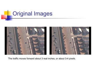
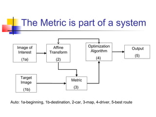
1) The document describes the mutual information metric, which is used to evaluate the similarity between two images after an affine transformation. 2) It discusses evaluating the metric based on factors like execution time, speed, and quality of the optimization. It also examines the relationship between image size and computation time. 3) The document explores sub-pixel resolution with the metric and analyzing histograms of the original and transformed images to evaluate the mapping between them. It considers future directions like using the histogram to determine the next transform.

1. The Mutual Information Metric
By Mike, and Vishal

2. Agenda
 Assumptions
 Original Images
 Flowchart
 Evaluating this
Metric
 Image Size vs.
Execution
 Sub-Pixel
Resolution
 Histograms
 Self
 Neighbor
 Difference
 Future Directions
 Questions

3. Assumptions
 Rigid transform
 No x-scale
 No y-scale
 x-translation
 y-translation
 rotation
 Only two pictures
 Traffic 001
 Traffic 024

4. Original Images
The traffic moves forward about 3 real inches, or about 3-4 pixels.

5. The Metric is part of a system
Image of
Interest
(1a)
Target
Image
(1b)
Affine
Transform
(2)
Optimization
Algorithm
(4)
Metric
(3)
Output
(5)
Auto: 1a-beginning, 1b-destination, 2-car, 3-map, 4-driver, 5-best route

6. Evaluating this Metric
 Price
 Execution time
 Improve Optimization
 Speed
 Quality
 Optimal Point
 Find Direction
 Find Locus
 Optimization Quality
 Sub-Pixel Resolution
 Error Tolerance

7. Image Size vs. Execution time
Computation Time vs. Image Size
y=2E-11x 2
+4E-06x+0.2765
R2
=0.9425
y=0.3131e 1E-05x
R2
=0.916
0
0.2
0.4
0.6
0.8
1
1.2
0 20000 40000 60000 80000 100000
Numberof Pixels
Computation Time
Series1
Series2
Poly.(Series1)
Expon.(Series2)
Transition from polynomial to exponential time
this happens around (140x140) pixels
In Matlab there is a destabilization around 20,000 pixels (140x140)
Notes: this data has already had about 10 outliers culled, and was done on p4 2.25Ghz w/256Mb Ram

8. Sub-Pixel Resolution
Given:
step = 0.1 pixel
Question:
How does MI vary
across boundary?
Results:
Near origin the
boundary varies
sharply at pixel
edges

9. Local Region

10. Sub-Pixel Resolution
Linear Interp
Pixel Min
Sub-Pixel Min

11. Sub-Pixel Resolution
 Poor Near Origin
 Ballasting?
 Valid away from origin
 Great between pixels
 Interpolation dependent
 Linear
 Others?
http://citeseer.ist.psu.edu/shekarforoush96subpixel.html

12. Error Tolerance
 Local extrema
 Many
 global max
 Single
 Large/clear
 Mixed results

13. Self Histogram
Pure Diagonal
Artifact ?

14. Neighbor Histogram
Fuzzy Diagonal

15. Difference in the histograms
• Note the transition in the diagonal.
• The “perfect” translation moves off-diagonal elements to make a strongly
diagonally dominant histogram
Top View
3-d View

16. Distance between mappings
Red and Green are highest distance, blue is least.
The aspect ratio of the roofs, sidewalks, and shadows is most informative.

17. Cleaner Dist between maps

18. Conclusions
 They say about golf:
 Drive for show, putt for dough
 MI is terrible for driving
 Many local maxima/minima
 High computational overhead
 MI is great for putting
 Sub-pixel resolution

19. Future Directions
 Can we determine the next transform based
on the histogram?
 Jacobi or Gauss-Seidel
 An inverse mapping from the histogram
 Diagonalization
 How well does this apply to point matching
algorithms?
 Inverse Histogram distance as a window?

20. Any Questions?