Vision Algorithms

1. VISION ALGORITHMS
Archana D
25249691142

2. INTRODUCTION TO MACHINE VISION
 Machine vision is the computational process of converting images captured by
cameras into meaningful information that can be used for decision-making,
measurement, automation, and control. Unlike computer graphics, which synthesizes
images, machine vision analyzes them.
Machine vision systems are widely used in:
 Industrial automation
 Robotics and navigation
 Quality inspection
 Medical imaging
 Metrology
 Surveillance

3. A MACHINE VISION PIPELINE
 Image Acquisition
 Image Enhancement
 Segmentation
 Feature Extraction
 Classification / Decision Making

4. IMAGE DATA STRUCTURES
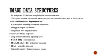
 An image is a 2D discrete sampling of a continuous scene.
 Each pixel stores a radiometric value proportional to the incident light at that location.
Pixel and Gray Level Representation
 A pixel stores intensity values that represent:
 Energy falling on the sensor
 Integration over exposure time
Sensor’s electronic response
 Gray level quantization typically uses:
 8-bit (0–255) – most common
 10-bit, 12-bit, 14-bit – industrial cameras
 16-bit – scientific cameras
 Higher bit depth = higher dynamic range.

5. IMAGE TYPES IN MACHINE VISION
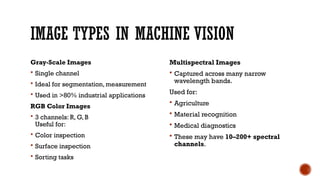
Gray-Scale Images
 Single channel
 Ideal for segmentation, measurement
 Used in >80% industrial applications
RGB Color Images
 3 channels: R, G, B
Useful for:
 Color inspection
 Surface inspection
 Sorting tasks
Multispectral Images
 Captured across many narrow
wavelength bands.
Used for:
 Agriculture
 Material recognition
 Medical diagnostics
 These may have 10–200+ spectral
channels.

6. IMAGE AS AN ARRAY OF CHANNELS
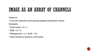
image as:
 A set of k channels, each storing sampled radiometric values.
Examples:
 Gray image k = 1
→
 RGB k = 3
→
 Multispectral k = N (N > 10)
→
 Each channel is stored in a 2D matrix.

7. REGIONS
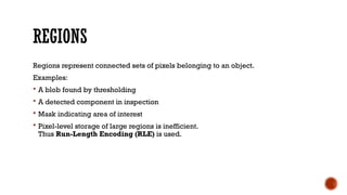
Regions represent connected sets of pixels belonging to an object.
Examples:
 A blob found by thresholding
 A detected component in inspection
 Mask indicating area of interest
 Pixel-level storage of large regions is inefficient.
Thus Run-Length Encoding (RLE) is used.

8. RUN-LENGTH ENCODING (RLE)
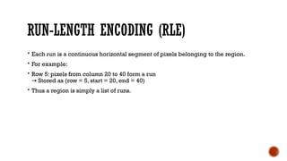
 Each run is a continuous horizontal segment of pixels belonging to the region.
 For example:
 Row 5: pixels from column 20 to 40 form a run
Stored as (row = 5, start = 20, end = 40)
→
 Thus a region is simply a list of runs.

9. ADVANTAGES OF RLE
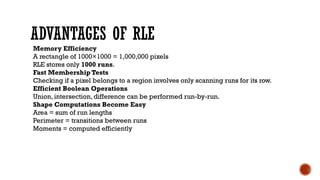
Memory Efficiency
A rectangle of 1000×1000 = 1,000,000 pixels
RLE stores only 1000 runs.
Fast Membership Tests
Checking if a pixel belongs to a region involves only scanning runs for its row.
Efficient Boolean Operations
Union, intersection, difference can be performed run-by-run.
Shape Computations Become Easy
Area = sum of run lengths
Perimeter = transitions between runs
Moments = computed efficiently

10. SUB-PIXEL PRECISE CONTOURS
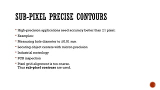
 High-precision applications need accuracy better than ±1 pixel.
 Examples:
 Measuring hole diameter to ±0.01 mm
 Locating object centers with micron precision
 Industrial metrology
 PCB inspection
 Pixel grid alignment is too coarse.
Thus sub-pixel contours are used.

11. WHY PIXEL PRECISION IS NOT ENOUGH
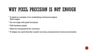
 A pixel is a sample of an underlying continuous signal.
Real edges:
 Do not align with pixel locations
 Fall between pixels
 Must be interpolated for accuracy
 If edges are used directly at pixel accuracy, measurement errors accumulate.

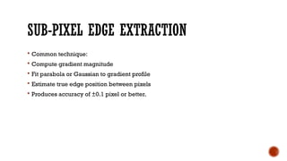
12. SUB-PIXEL EDGE EXTRACTION
 Common technique:
 Compute gradient magnitude
 Fit parabola or Gaussian to gradient profile
 Estimate true edge position between pixels
 Produces accuracy of ±0.1 pixel or better.

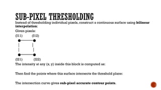
13. SUB-PIXEL THRESHOLDING
Instead of thresholding individual pixels, construct a continuous surface using bilinear
interpolation:
Given pixels:
(I11) (I12)
●──────●
│ │
│ │
●──────●
(I21) (I22)
The intensity at any (x, y) inside this block is computed as:
Then find the points where this surface intersects the threshold plane:
The intersection curve gives sub-pixel accurate contour points.

14. SUB-PIXEL CONTOUR REPRESENTATION
A contour is stored as:
 All coordinates are floating-point, not integers.
 Types of contours:
 Open contours
 Closed contours
 Branching contours (junction nodes)

15. IMAGE ENHANCEMENT
 Image enhancement improves the visual quality of an image or prepares it for
further processing (like segmentation or measurement).
Enhancement does not increase actual information, but makes important
features easier to analyze.
Enhancement techniques fall into three major categories:
 Point Operations (Pixel-based)
 Neighborhood Operations (Filtering / Smoothing)
 Frequency Domain Methods (Fourier-based enhancement)

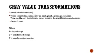
16. GRAY VALUE TRANSFORMATIONS
 (Point-Based Operations)
 These operate independently on each pixel, ignoring neighbors.
They modify only the intensity value, keeping the pixel location unchanged.
 General form:
Where
f = input image
g = transformed image
T = transformation function

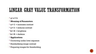
17. LINEAR GRAY VALUE TRANSFORMATION
 g=a f+b
⋅
 Meaning of Parameters
 a > 1 increases contrast
→
 a < 1 reduces contrast
→
 b > 0 brightens
→
 b < 0 darkens
→
 Applications
 Correcting under/over exposure
 Standardizing image contrast
 Preparing images for thresholding

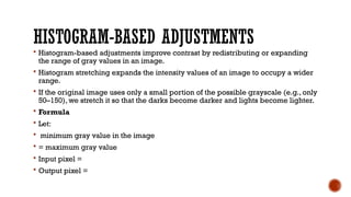
18. HISTOGRAM-BASED ADJUSTMENTS
 Histogram-based adjustments improve contrast by redistributing or expanding
the range of gray values in an image.
 Histogram stretching expands the intensity values of an image to occupy a wider
range.
 If the original image uses only a small portion of the possible grayscale (e.g., only
50–150), we stretch it so that the darks become darker and lights become lighter.
 Formula
 Let:
 minimum gray value in the image
 = maximum gray value
 Input pixel =
 Output pixel =

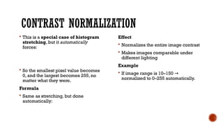
19. CONTRAST NORMALIZATION
 This is a special case of histogram
stretching, but it automatically
forces:
 So the smallest pixel value becomes
0, and the largest becomes 255, no
matter what they were.
Formula
 Same as stretching, but done
automatically:
Effect
 Normalizes the entire image contrast
 Makes images comparable under
different lighting
Example
 If image range is 10–150 →
normalized to 0–255 automatically.

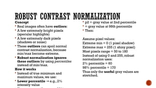
20. ROBUST CONTRAST NORMALIZATION
Concept
 Real images often have outliers:
 A few extremely bright pixels
(specular highlights)
 A few extremely dark pixels
(shadows or noise)
 These outliers can spoil normal
contrast normalization, because
min/max become extreme.
 Robust normalization ignores
these outliers by using percentiles
instead of min/max.
How it works
 Instead of true minimum and
maximum values, we use:
 Lower percentile e.g., 2%
→
intensity value
 p2​= gray value at 2nd percentile
 = gray value at 98th percentile
 Then:
Assume pixel values:
Extreme min = 0 (1 pixel shadow)
Extreme max = 255 (1 shiny pixel)
Most pixels range = 50 to 180
Instead of using 0 and 255, robust
normalization uses:
2% percentile = 60
98% percentile = 170
Thus only the useful gray values are
stretched.

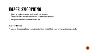
21. IMAGE SMOOTHING
 Used to reduce noise and small variations.
Essential before segmentation or edge detection.
 Neighborhood-Based Operations
Linear Filters
 Linear filters replace each pixel with a weighted sum of neighboring pixels.

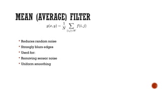
22. MEAN (AVERAGE) FILTER
 Reduces random noise
 Strongly blurs edges
 Used for:
 Removing sensor noise
 Uniform smoothing

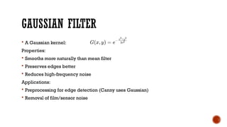
23. GAUSSIAN FILTER
 A Gaussian kernel:
Properties:
 Smooths more naturally than mean filter
 Preserves edges better
 Reduces high-frequency noise
Applications:
 Preprocessing for edge detection (Canny uses Gaussian)
 Removal of film/sensor noise

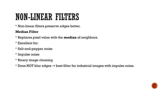
24. NON-LINEAR FILTERS
 Non-linear filters preserve edges better.
Median Filter
 Replaces pixel value with the median of neighbors.
 Excellent for:
 Salt-and-pepper noise
 Impulse noise
 Binary image cleaning
 Does NOT blur edges best filter for industrial images with impulse noise.
→

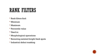
25. RANK FILTERS
 Rank filters find:
 Minimum
 Maximum
 Percentile value
 Used in:
 Morphological operations
 Removing isolated bright/dark spots
 Industrial defect masking

26. FREQUENCY DOMAIN ENHANCEMENT
 Image enhancement in the frequency domain modifies an image by changing its
frequency components (low frequencies, high frequencies, periodic patterns).
 To do this, we use the Fourier Transform.

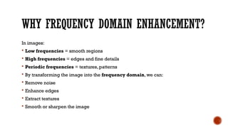
27. WHY FREQUENCY DOMAIN ENHANCEMENT?
In images:
 Low frequencies = smooth regions
 High frequencies = edges and fine details
 Periodic frequencies = textures, patterns
 By transforming the image into the frequency domain, we can:
 Remove noise
 Enhance edges
 Extract textures
 Smooth or sharpen the image

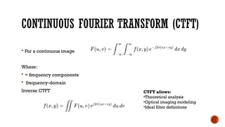
28. CONTINUOUS FOURIER TRANSFORM (CTFT)
 For a continuous image
Where:
 = frequency components
 frequency-domain
Inverse CTFT CTFT allows:
•Theoretical analysis
•Optical imaging modeling
•Ideal filter definitions

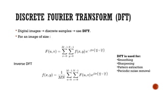
29. DISCRETE FOURIER TRANSFORM (DFT)
 Digital images discrete samples use
→ → DFT.
 For an image of size :
DFT is used for:
•Smoothing
•Sharpening
•Pattern extraction
•Periodic noise removal

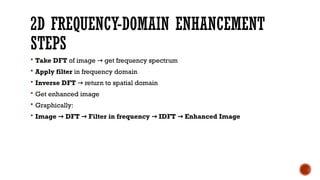
30. 2D FREQUENCY-DOMAIN ENHANCEMENT
STEPS
 Take DFT of image get frequency spectrum
→
 Apply filter in frequency domain
 Inverse DFT return to spatial domain
→
 Get enhanced image
 Graphically:
 Image DFT Filter in frequency IDFT Enhanced Image
→ → → →

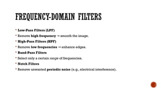
31. FREQUENCY-DOMAIN FILTERS
 Low-Pass Filters (LPF)
 Remove high frequency smooth the image.
→
 High-Pass Filters (HPF)
 Remove low frequencies enhance edges.
→
 Band-Pass Filters
 Select only a certain range of frequencies.
 Notch Filters
 Remove unwanted periodic noise (e.g., electrical interference).

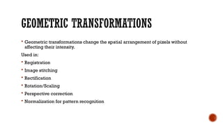
32. GEOMETRIC TRANSFORMATIONS
 Geometric transformations change the spatial arrangement of pixels without
affecting their intensity.
Used in:
 Registration
 Image stitching
 Rectification
 Rotation/Scaling
 Perspective correction
 Normalization for pattern recognition

33. BASIC TRANSFORMATIONS
Translation
Scaling
Rotation

34. AFFINE TRANSFORMATION
 Matrix A includes:
 Rotation
 Scaling
 Shear
 Properties
 Parallel lines remain parallel
 Ratios of distances along lines remain constant

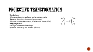
35. PROJECTIVE TRANSFORMATION
Used when:
•Camera observes a planar surface at an angle
•Perspective distortion must be removed
•License plates, documents, labels must be rectified
Key properties
•Straight lines remain straight
•Parallel lines may not remain parallel

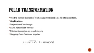
36. POLAR TRANSFORMATION
 Used to convert circular or rotationally symmetric objects into linear form.
 Applications
 Inspection of bottle caps
 Label verification on cans
 Printing inspection on round objects
 Mapping from Cartesian to polar:

37. INTRODUCTION TO SEGMENTATION
 Segmentation divides an image into meaningful units such as:
 Objects
 Background
 Edges
 Contours
 Regions
 Two main classes:
 Region-Based Segmentation
 Contour-Based Segmentation

38. THRESHOLDING
 Thresholding is one of the simplest and most widely used segmentation
techniques.
Global Thresholding
 A constant threshold T is applied:
 Used when:
 Object and background have distinct intensities
 Illumination is uniform

39. AUTOMATIC THRESHOLD SELECTION
 When illumination varies, fixed threshold fails.
Automatic thresholding uses histogram analysis to select best threshold.
 Common methods:
 Valley detection in histogram
 Isodata method (iterative)
 Otsu’s method (maximizes inter-class variance)

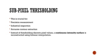
40. SUB-PIXEL THRESHOLDING
 This is crucial for:
 Precision measurement
 Industrial inspection
 Accurate contour extraction
 Instead of thresholding discrete pixel values, a continuous intensity surface is
reconstructed using bilinear interpolation.

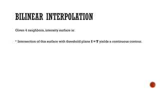
41. BILINEAR INTERPOLATION
Given 4 neighbors, intensity surface is:
 Intersection of this surface with threshold plane I = T yields a continuous contour.

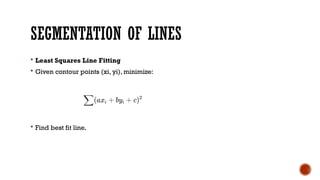
42. SEGMENTATION OF LINES
 Least Squares Line Fitting
 Given contour points (xi, yi), minimize:
 Find best fit line.

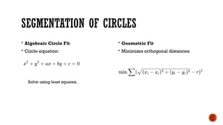
43. SEGMENTATION OF CIRCLES
 Algebraic Circle Fit
 Circle equation:
 Geometric Fit
 Minimizes orthogonal distances:
Solve using least squares.

44. SEGMENTATION OF ELLIPSES
 Ellipse equation:
Used in:
•Bearing inspection
•Hole inspection
•Coin & washer inspection
Parameters estimated via algebraic or geometric least
squares.

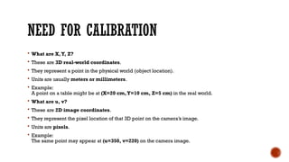
45. NEED FOR CALIBRATION
 What are X,Y, Z?
 These are 3D real-world coordinates.
 They represent a point in the physical world (object location).
 Units are usually meters or millimeters.
 Example:
A point on a table might be at (X=20 cm,Y=10 cm, Z=5 cm) in the real world.
 What are u, v?
 These are 2D image coordinates.
 They represent the pixel location of that 3D point on the camera’s image.
 Units are pixels.
 Example:
The same point may appear at (u=350, v=220) on the camera image.

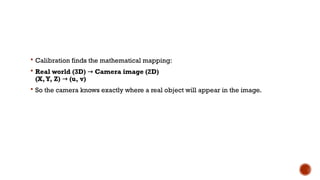
46.  Calibration finds the mathematical mapping:
 Real world (3D) → Camera image (2D)
(X,Y, Z) → (u, v)
 So the camera knows exactly where a real object will appear in the image.

47. CAMERA PARAMETERS
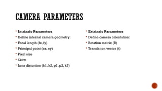
 Intrinsic Parameters
 Define internal camera geometry:
 Focal length (fx, fy)
 Principal point (cx, cy)
 Pixel size
 Skew
 Lens distortion (k1, k2, p1, p2, k3)
 Extrinsic Parameters
 Define camera orientation:
 Rotation matrix (R)
 Translation vector (t)

48. CALIBRATION PROCESS
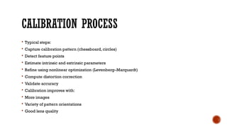
 Typical steps:
 Capture calibration pattern (chessboard, circles)
 Detect feature points
 Estimate intrinsic and extrinsic parameters
 Refine using nonlinear optimization (Levenberg–Marquardt)
 Compute distortion correction
 Validate accuracy
 Calibration improves with:
 More images
 Variety of pattern orientations
 Good lens quality

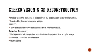
49. STEREO VISION & 3D RECONSTRUCTION
 Stereo uses two cameras to reconstruct 3D information using triangulation.
 Inspired by human binocular vision.
STEREO
 Two cameras observe same scene from two viewpoints.
Epipolar Geometry
 Each point in left image lies on a horizontal epipolar line in right image
 Reduces 2D search 1D search
→
 GEOMETRY

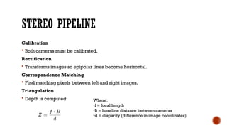
50. STEREO PIPELINE
Calibration
 Both cameras must be calibrated.
Rectification
 Transforms images so epipolar lines become horizontal.
Correspondence Matching
 Find matching pixels between left and right images.
Triangulation
 Depth is computed: Where:
•f = focal length
•B = baseline distance between cameras
•d = disparity (difference in image coordinates)

51. APPLICATIONS OF STEREO VISION
3D measurement
Robot navigation
Obstacle detection
Autonomous vehicles
3D scanning
Industrial inspection

52. VISION SENSORS
 Vision sensors are compact devices combining:
 Imaging optics
 Sensor
 On-board image processing
 Output interfaces
 They function as “smart cameras.”

53. COMPONENTS OF A VISION SENSOR
Lens
Image sensor (CCD/CMOS)
Processor (DSP/FPGA)
Illumination
Software for detection/measurement
Communication (Ethernet, RS-485, Fieldbus)

54. THANK YOU