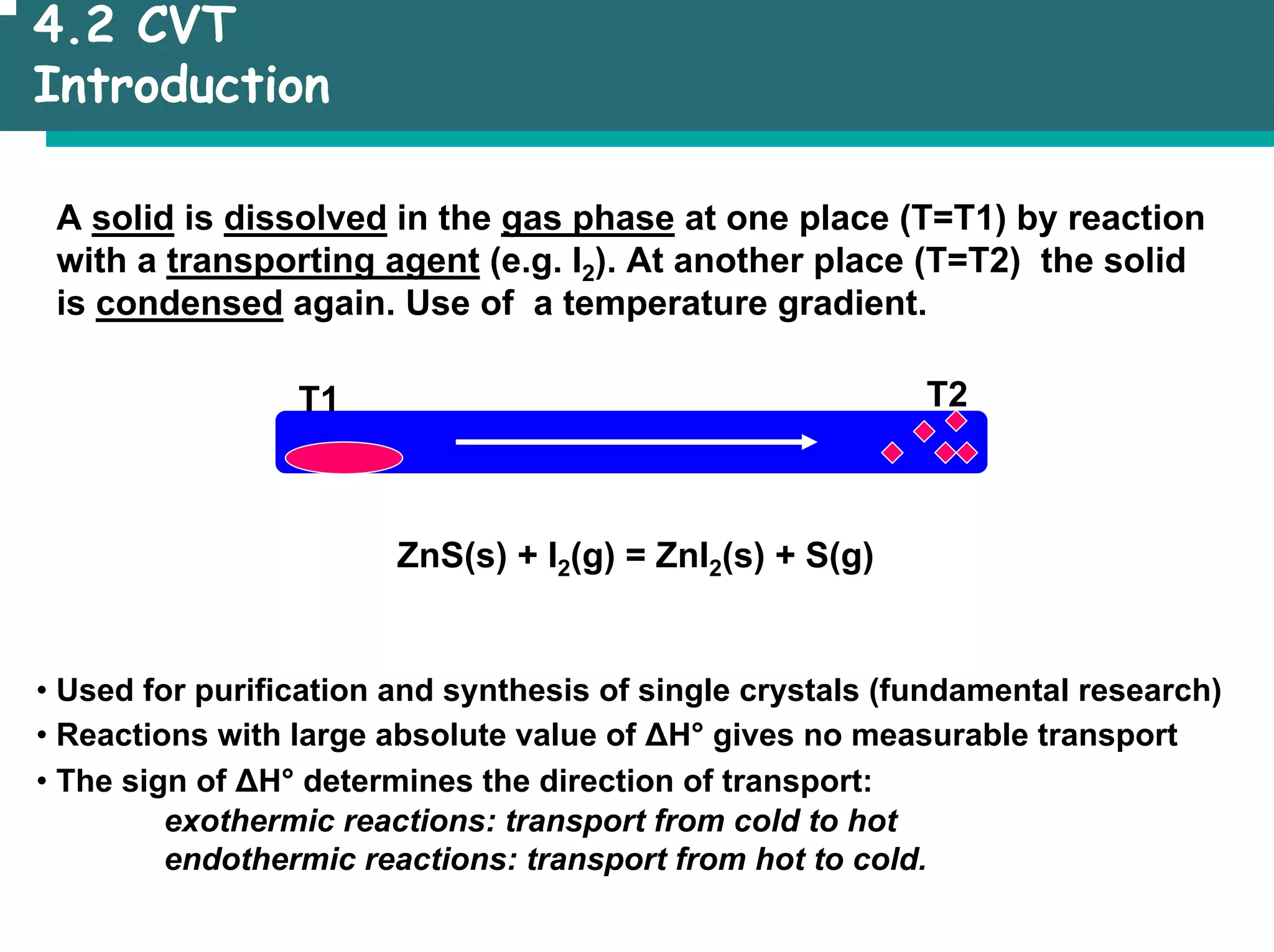
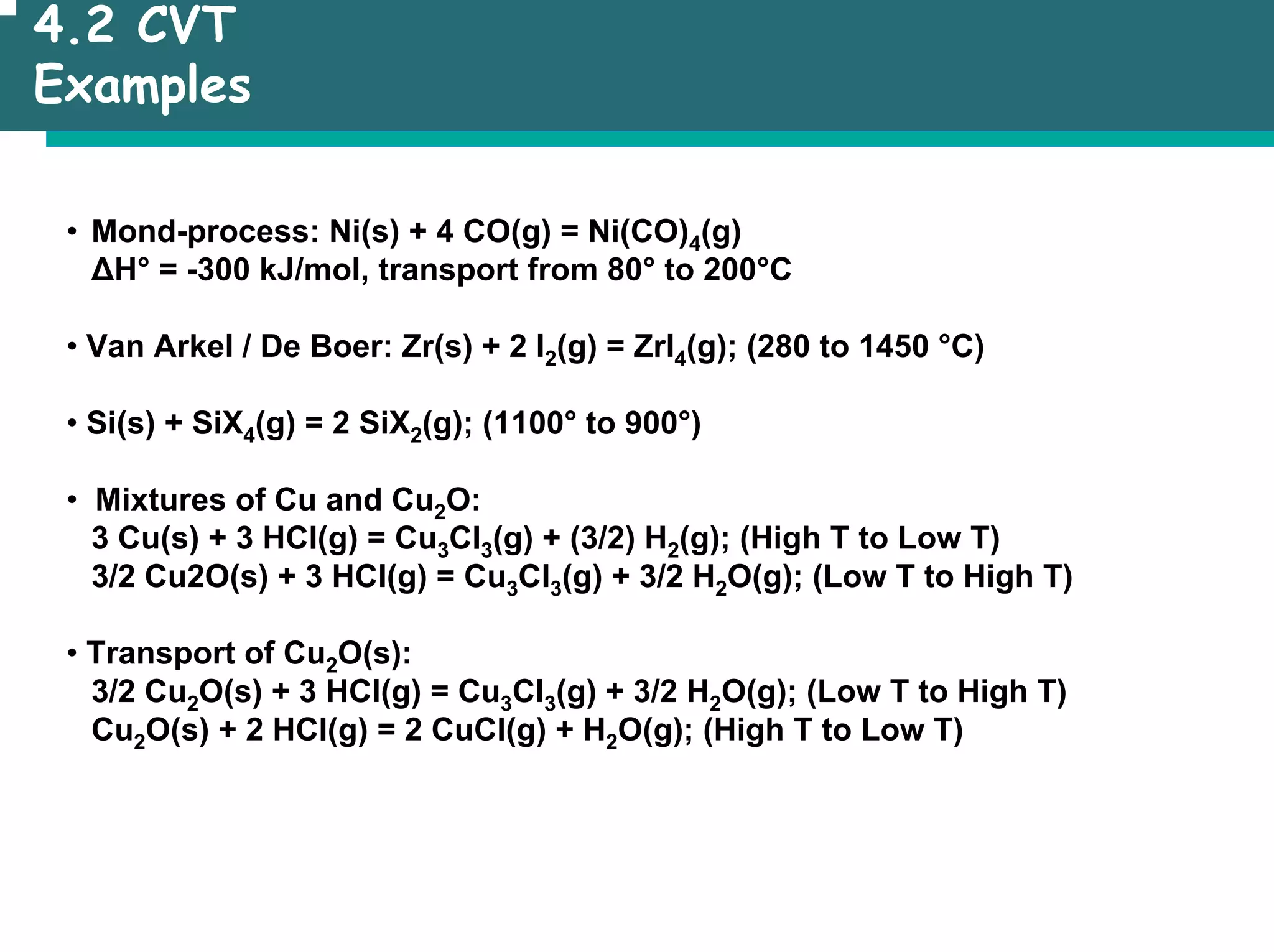
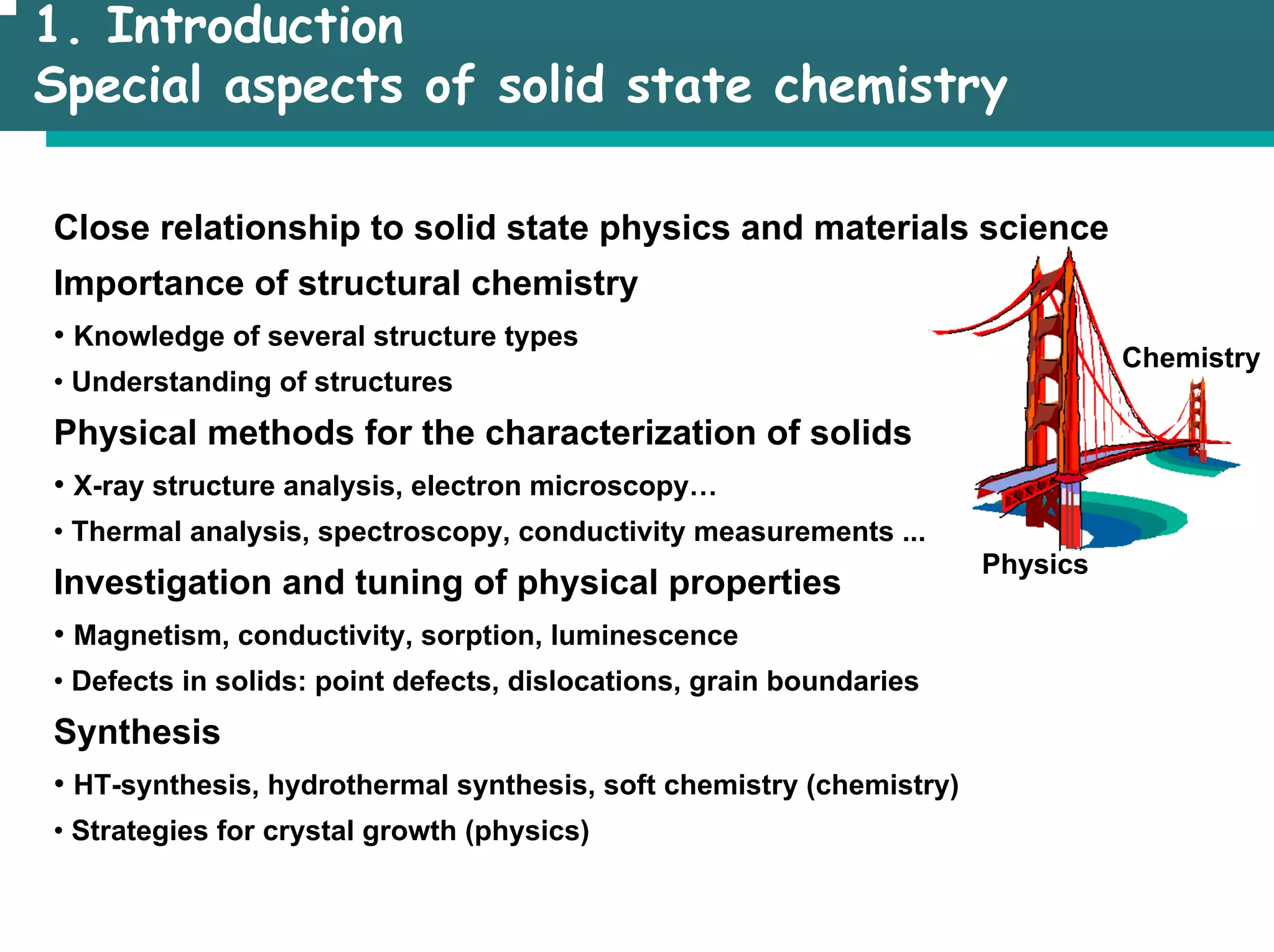
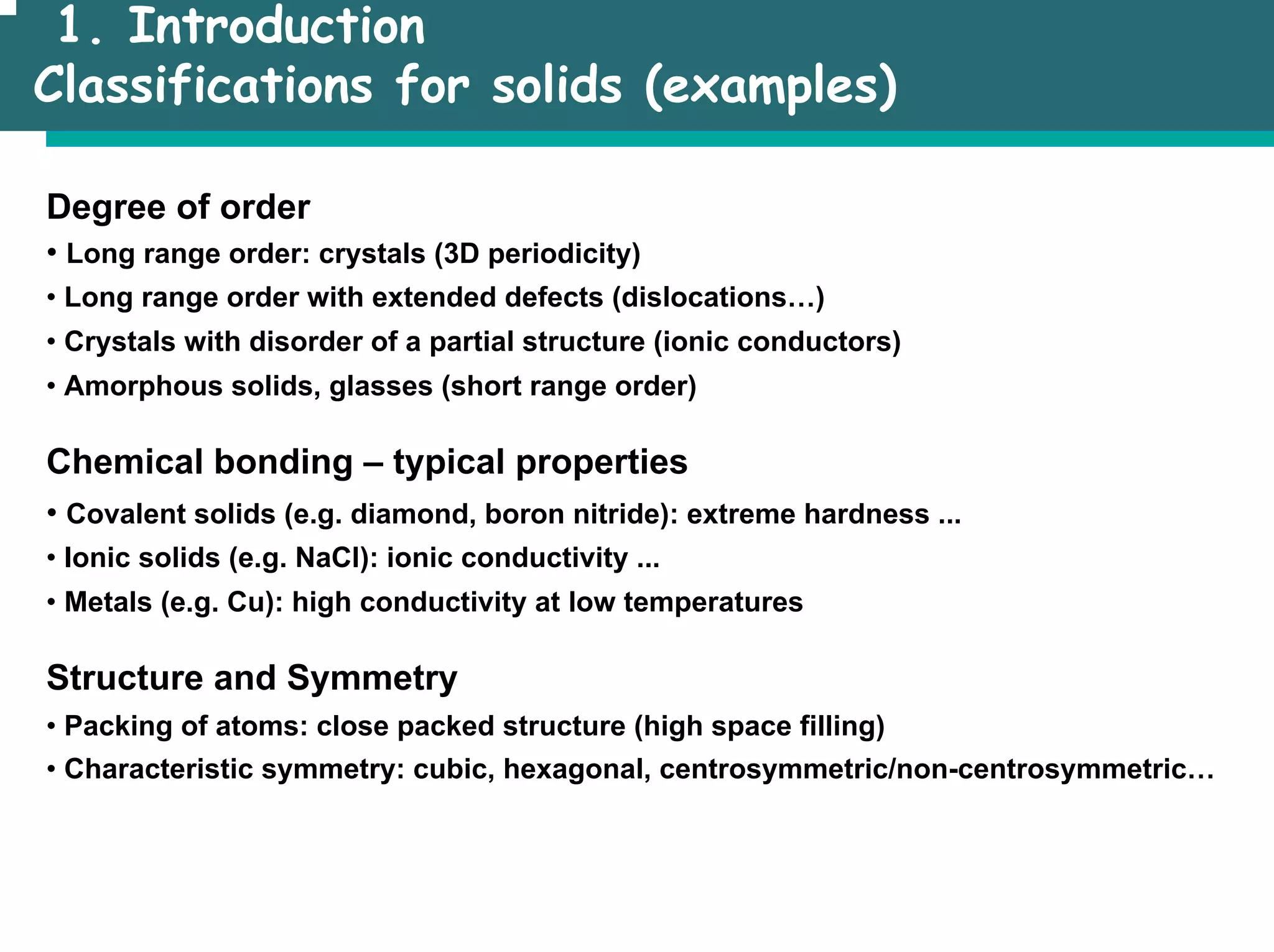
The document outlines the structures and properties of solids, including classification based on degree of order and various bonding types. It covers basics of solid-state chemistry, characterization methods, and synthesis techniques alongside visualizations of crystal structures such as close-packed arrangements. Key examples include the properties of covalent, ionic, and metallic solids, as well as specific structure types and rules like Pauling's rules.


![2.1 Basics of Structures
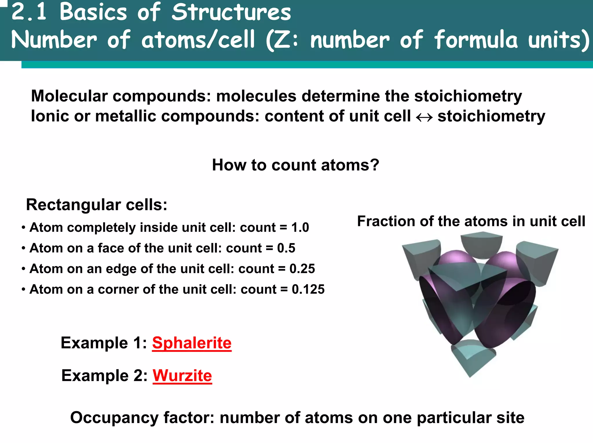
Fractional coordinates (position of the atoms)
• possible values for x, y, z: [0; 1], atoms are multiplied by translations
• atoms are generated by symmetry elements (see SSC)
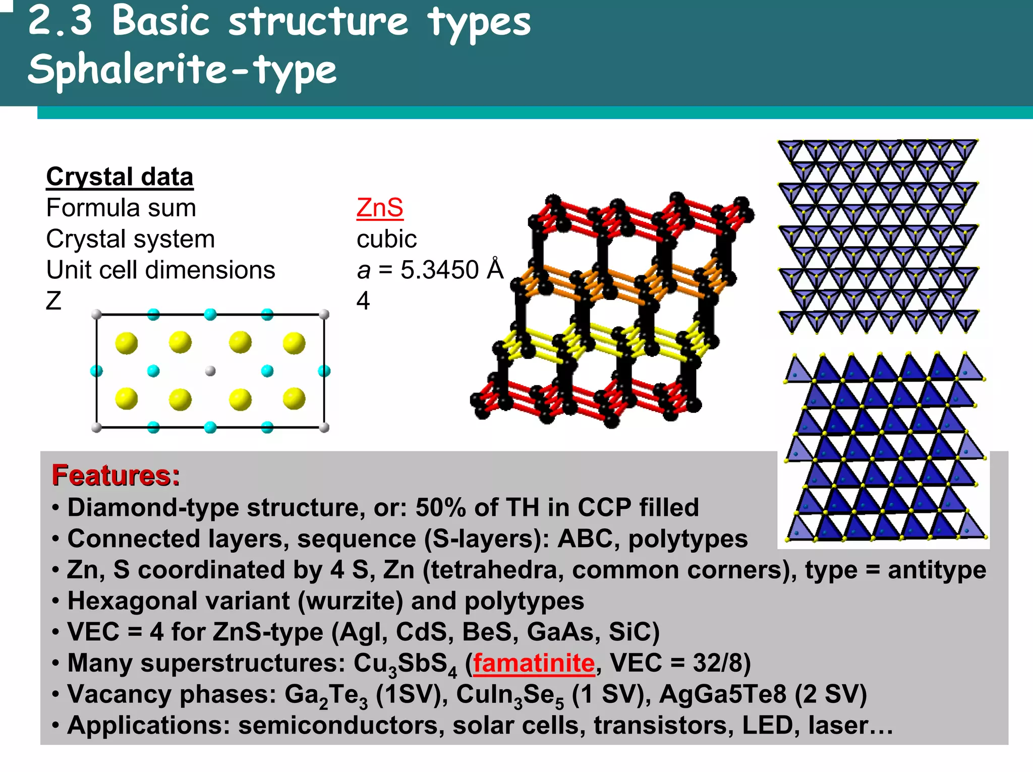
• Example: Sphalerite (ZnS)
1/2
1/2
1/2
• Equivalent points are represented by one triplet only
• equivalent by translation
• equivalent by other symmetry elements (see SSC)](https://image.slidesharecdn.com/msestructureofsolids-230701184219-0c7b3232/75/MSE_Structure-of-solids-pdf-15-2048.jpg)
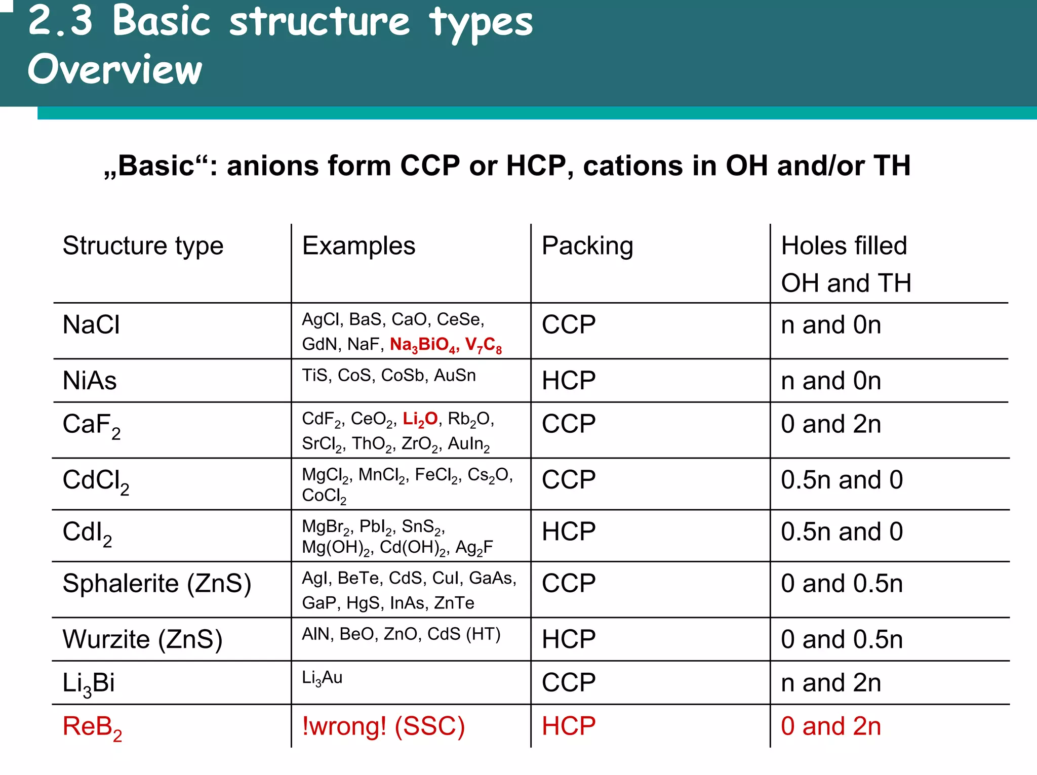
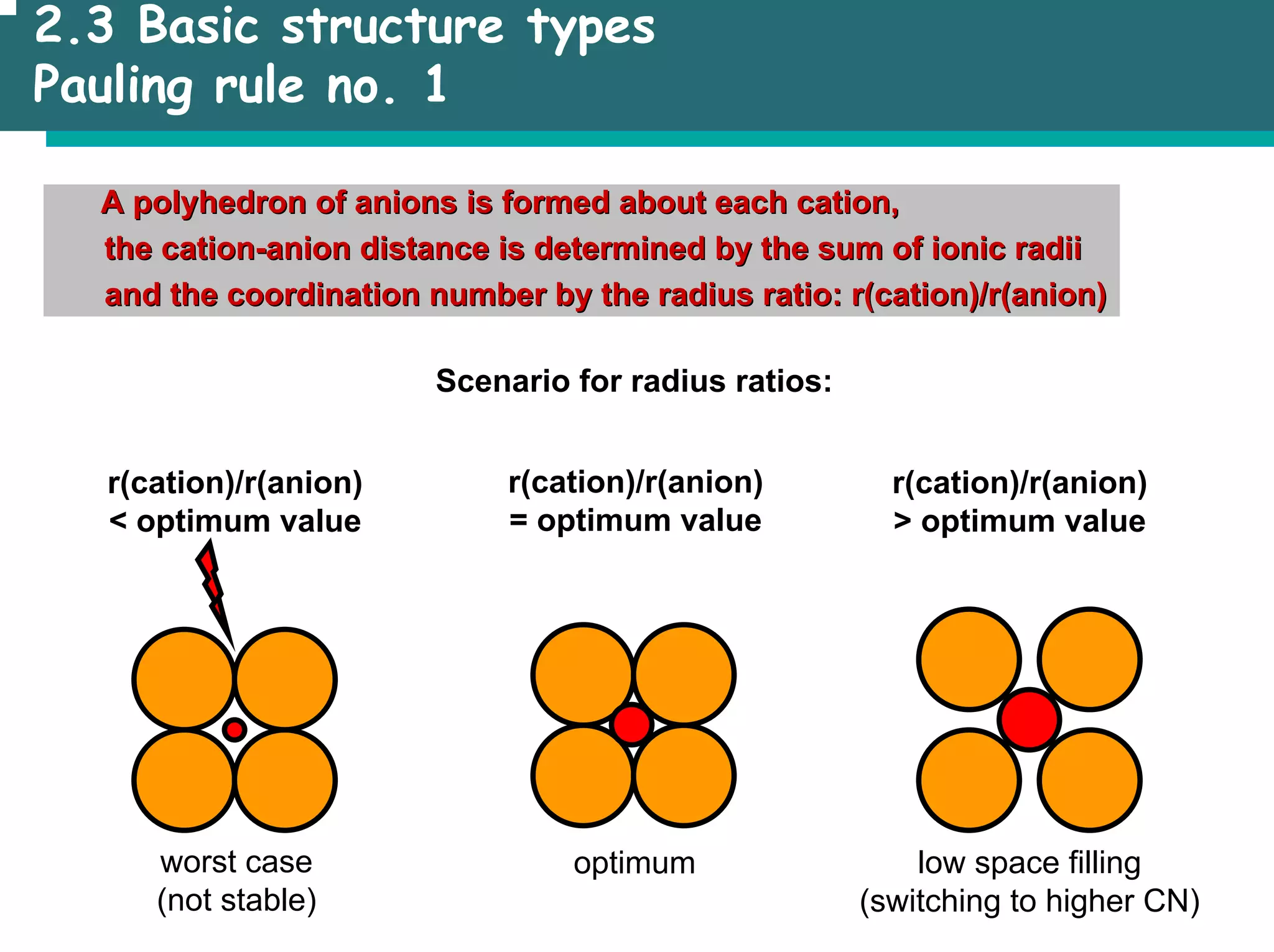
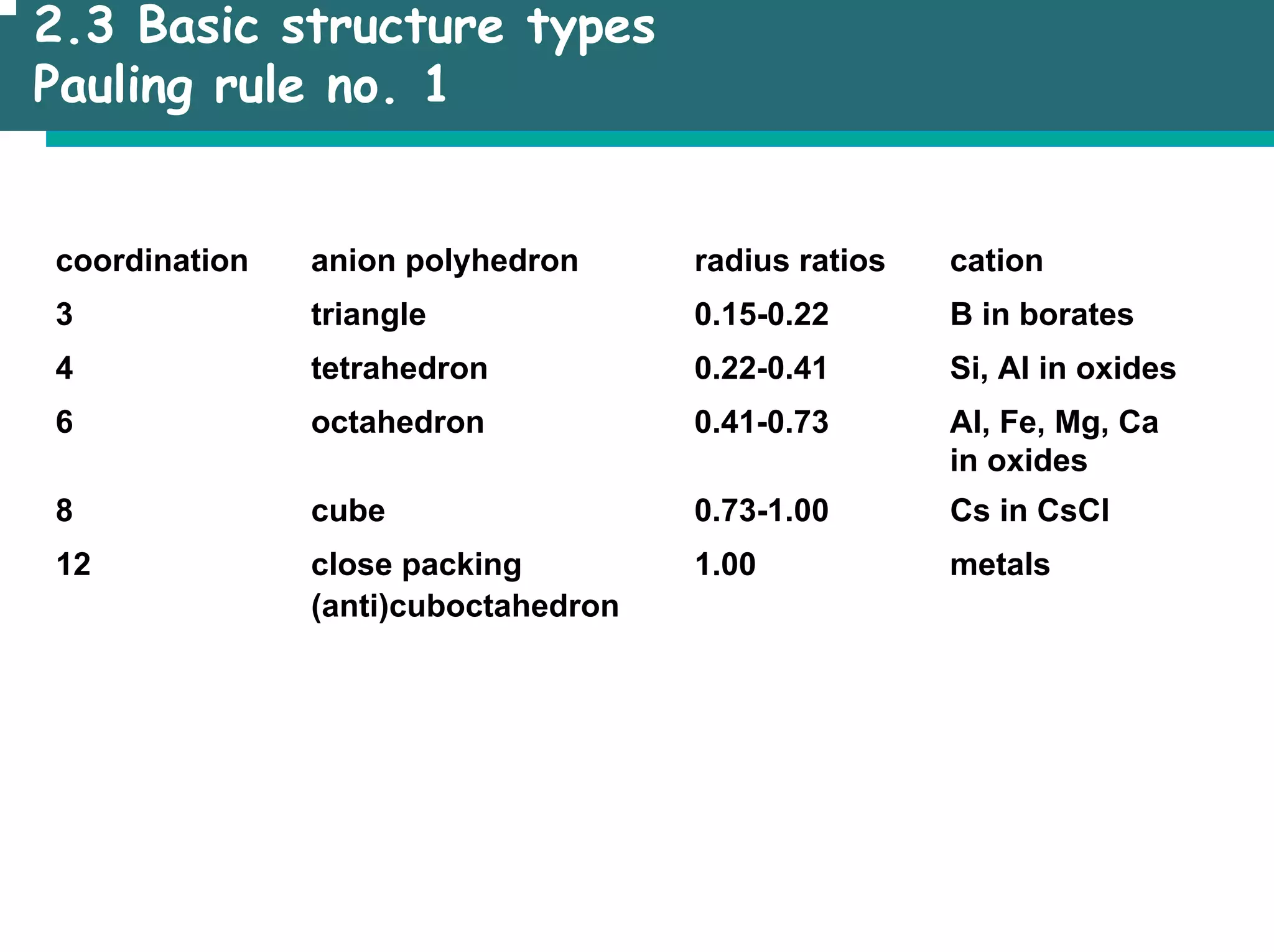
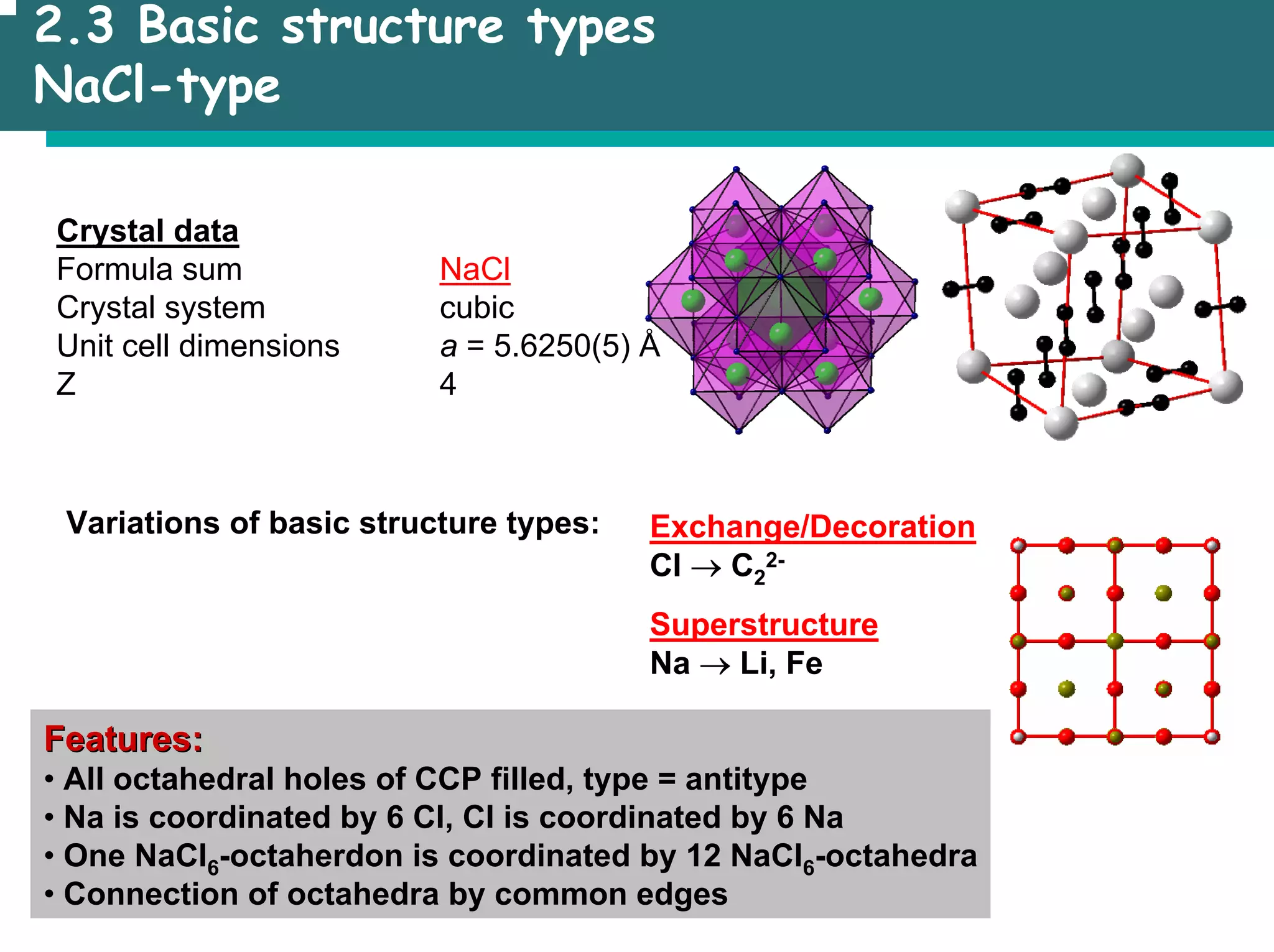
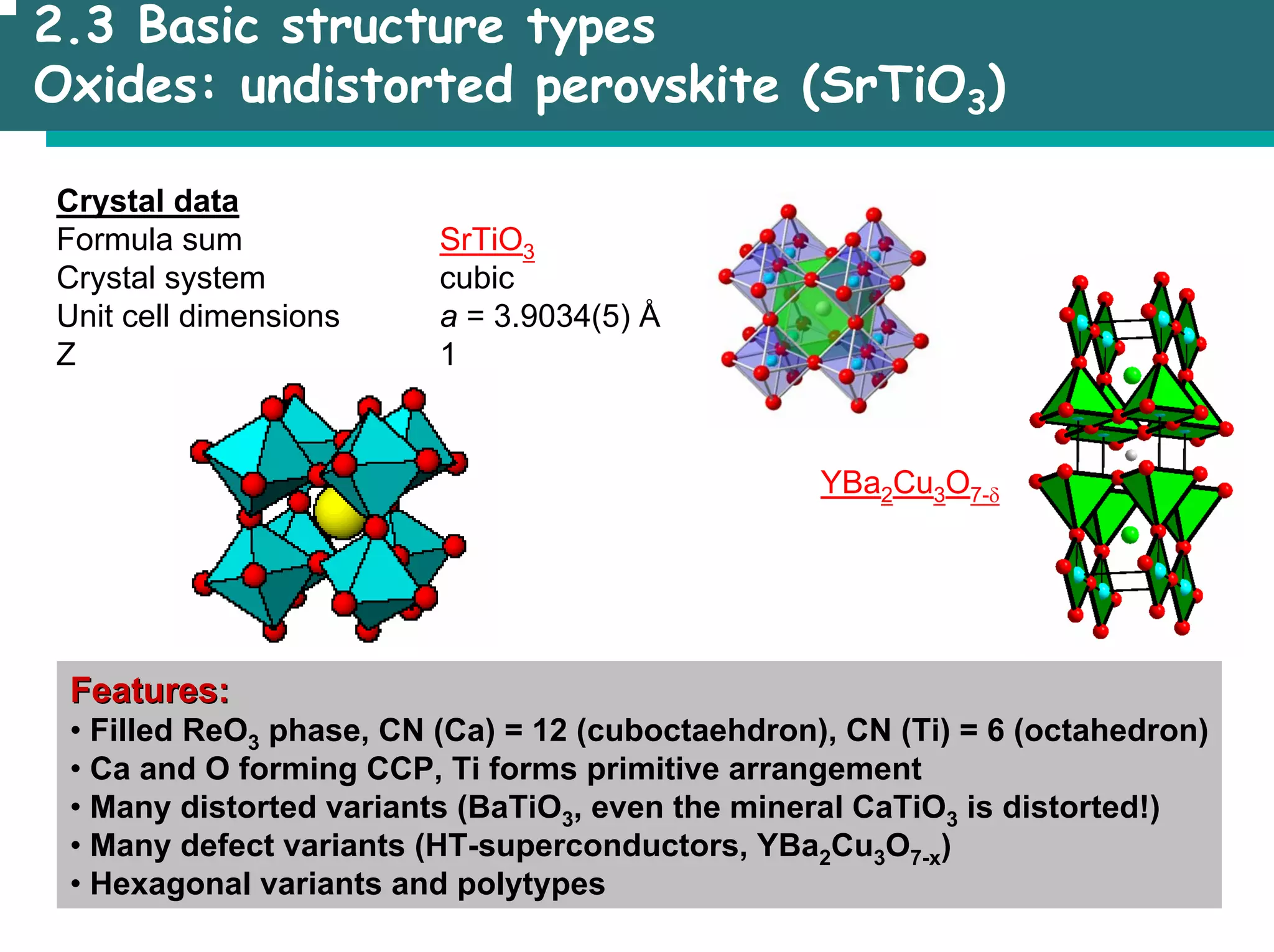
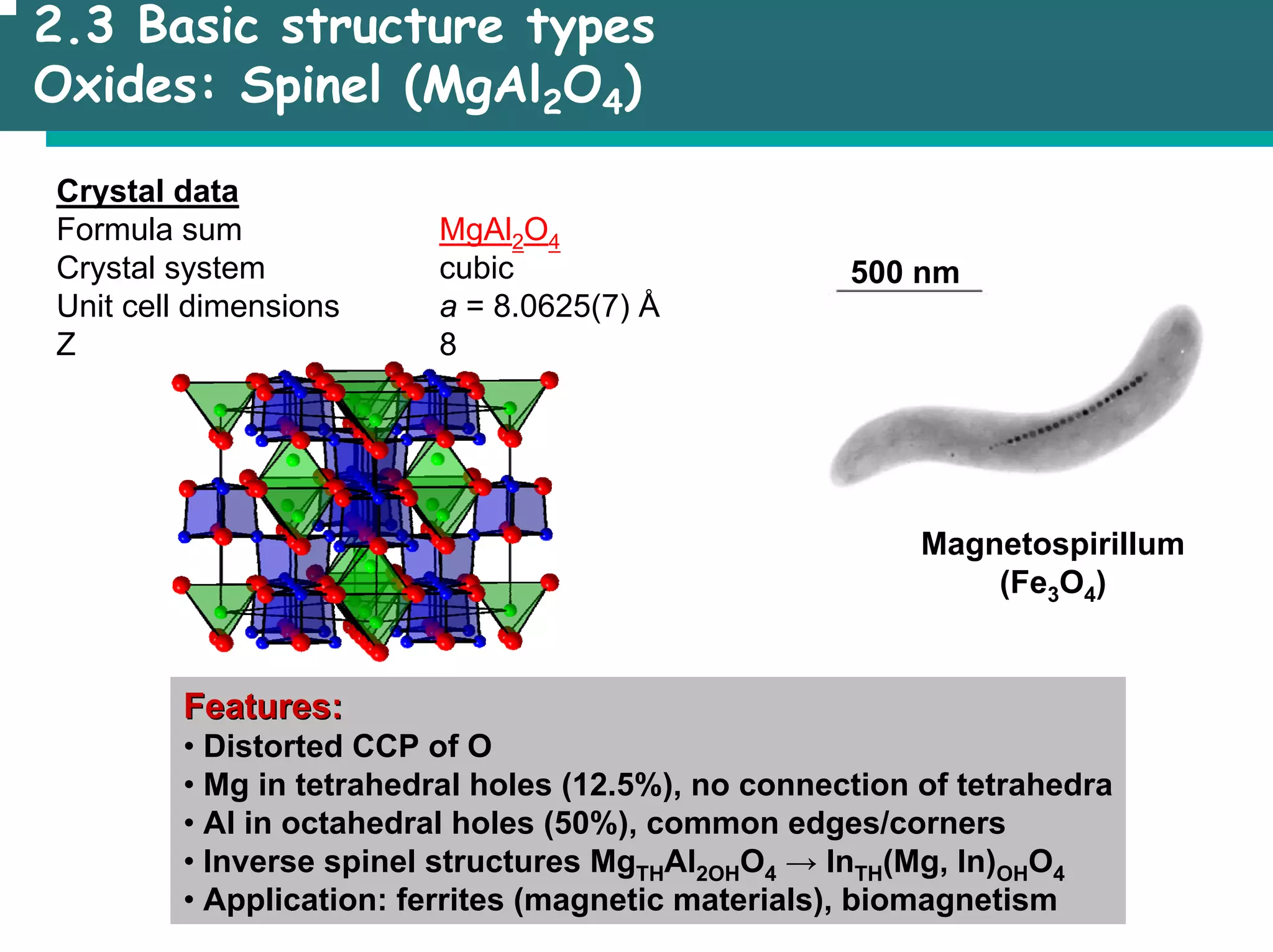
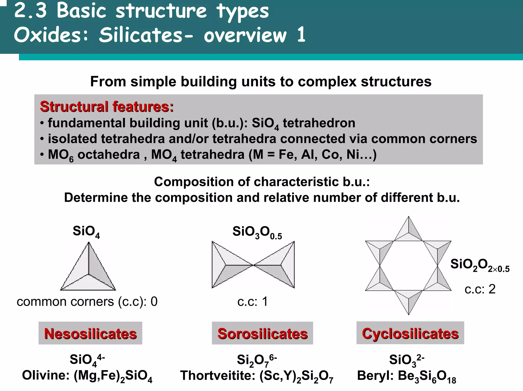
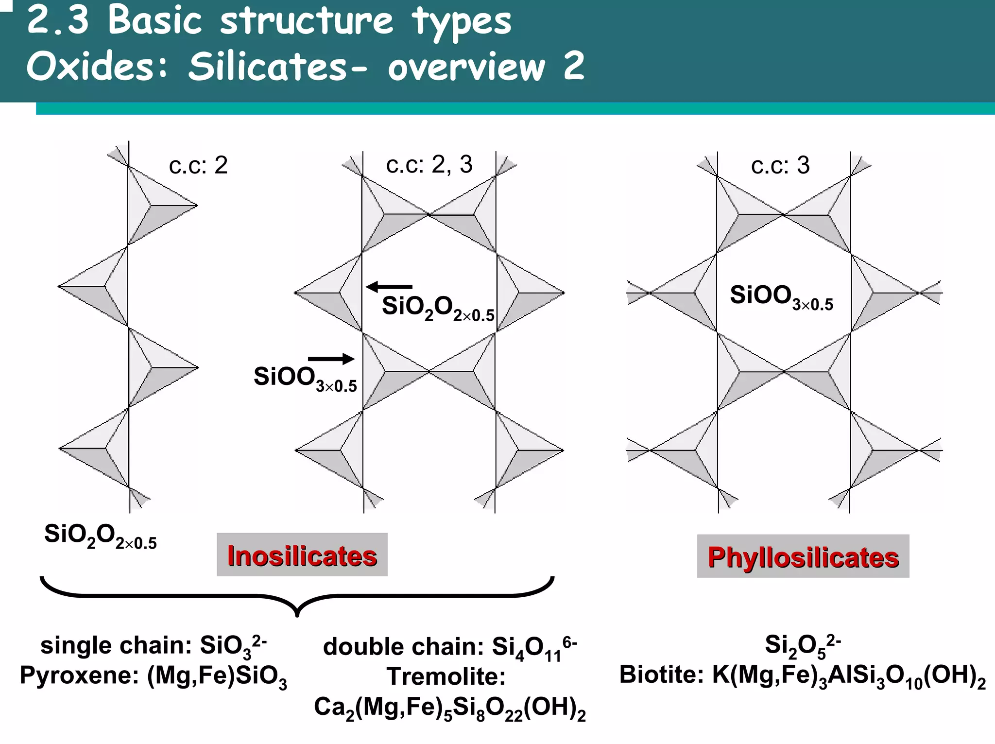
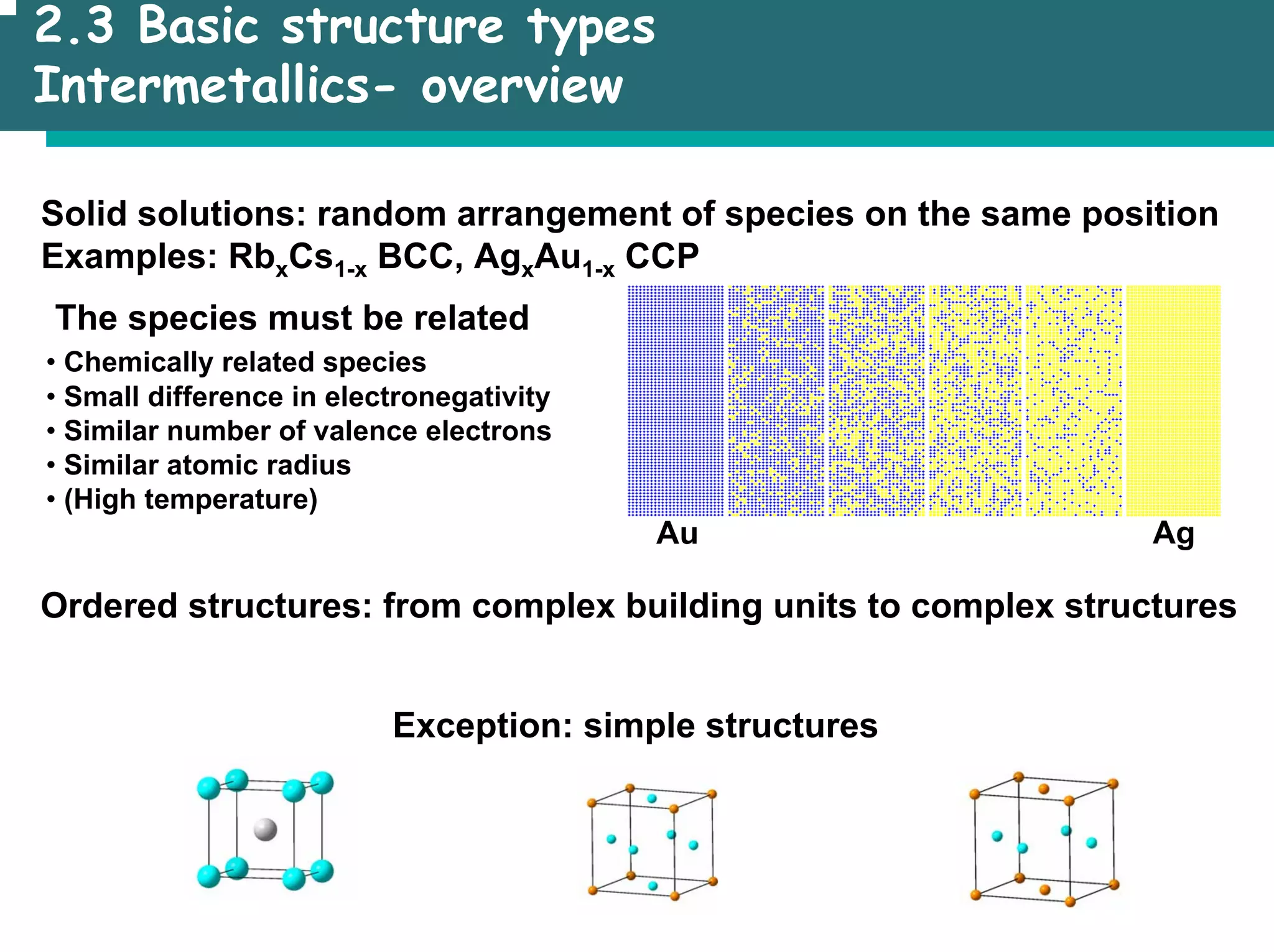
![2.3 Basic structure types
Oxides: Silicates- overview 3
Tectosilicates
Tectosilicates c.c: 4, SiO2, Faujasite: Ca28.5Al57Si135O384
Pores
•mH2O
[Si1-xAlxO2]
Ax/n
Pores
T (= Si, Al)O4-Tetrahedra sharing all corners,
isomorphous exchange of Si4+, charge compensation
x: Al content, charge of microporous framework, n: charge of A
Zeolites
• Alumosilicates with open channels or cages (d < 2 nm, “boiling stones”)
• Numerous applications: adsorbent, catalysis…](https://image.slidesharecdn.com/msestructureofsolids-230701184219-0c7b3232/75/MSE_Structure-of-solids-pdf-36-2048.jpg)

![4.1 Diffraction
Results of diffraction studies- Overview
Lattice parameters
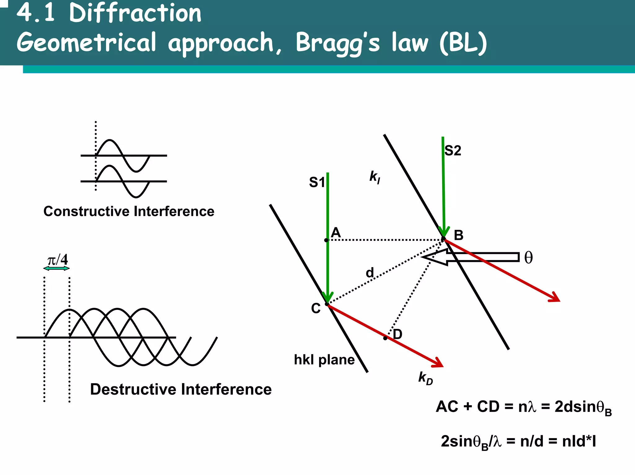
Position of the reflections (Bragg’s law), e. g. (1/d)2 = (1/a)2 [h2 + k2+ l2]
Symmetry of the structure
Intensity of the reflections and geometry of DP = symmetry of DP
Identification of samples (fingerprint)
Structure, fractional coordinates…:
Intensity of the reflections, quantitative analysis (solution and refinement)
Crystal size and perfection
Profile of the reflections
Special techniques
• Electron diffraction: highly significant data, SAED (DP of different areas of one crystal)
• Neutron diffraction: localization of H, analyses of magnetic structures
• Synchrotron: small crystals, large structures (protein structures)](https://image.slidesharecdn.com/msestructureofsolids-230701184219-0c7b3232/75/MSE_Structure-of-solids-pdf-42-2048.jpg)