Downloaded 29 times


![scikit-learn user guide, Release 0.16.0
1.2 Loading an example dataset
scikit-learn comes with a few standard datasets, for instance the iris and digits datasets for classification and the boston
house prices dataset for regression.
In the following, we start a Python interpreter from our shell and then load the iris and digits datasets. Our
notational convention is that $ denotes the shell prompt while >>> denotes the Python interpreter prompt:
$ python
>>> from sklearn import datasets
>>> iris = datasets.load_iris()
>>> digits = datasets.load_digits()
A dataset is a dictionary-like object that holds all the data and some metadata about the data. This data is stored in
the .data member, which is a n_samples, n_features array. In the case of supervised problem, one or more
response variables are stored in the .target member. More details on the different datasets can be found in the
dedicated section.
For instance, in the case of the digits dataset, digits.data gives access to the features that can be used to classify
the digits samples:
>>> print(digits.data)
[[ 0. 0. 5. ..., 0. 0. 0.]
[ 0. 0. 0. ..., 10. 0. 0.]
[ 0. 0. 0. ..., 16. 9. 0.]
...,
[ 0. 0. 1. ..., 6. 0. 0.]
[ 0. 0. 2. ..., 12. 0. 0.]
[ 0. 0. 10. ..., 12. 1. 0.]]
and digits.target gives the ground truth for the digit dataset, that is the number corresponding to each digit
image that we are trying to learn:
>>> digits.target
array([0, 1, 2, ..., 8, 9, 8])
Shape of the data arrays
The data is always a 2D array, shape (n_samples, n_features), although the original data may have
had a different shape. In the case of the digits, each original sample is an image of shape (8, 8) and can be
accessed using:
>>> digits.images[0]
array([[ 0., 0., 5., 13., 9., 1., 0., 0.],
[ 0., 0., 13., 15., 10., 15., 5., 0.],
[ 0., 3., 15., 2., 0., 11., 8., 0.],
[ 0., 4., 12., 0., 0., 8., 8., 0.],
[ 0., 5., 8., 0., 0., 9., 8., 0.],
[ 0., 4., 11., 0., 1., 12., 7., 0.],
[ 0., 2., 14., 5., 10., 12., 0., 0.],
[ 0., 0., 6., 13., 10., 0., 0., 0.]])
The simple example on this dataset illustrates how starting from the original problem one can shape the data for
consumption in scikit-learn.
4 Chapter 1. An introduction to machine learning with scikit-learn](https://image.slidesharecdn.com/scikit-learn0-150409112902-conversion-gate01/85/Scikit-learn-0-16-0-user-guide-14-320.jpg)
![scikit-learn user guide, Release 0.16.0
1.3 Learning and predicting
In the case of the digits dataset, the task is to predict, given an image, which digit it represents. We are given samples
of each of the 10 possible classes (the digits zero through nine) on which we fit an estimator to be able to predict the
classes to which unseen samples belong.
In scikit-learn, an estimator for classification is a Python object that implements the methods fit(X, y) and
predict(T).
An example of an estimator is the class sklearn.svm.SVC that implements support vector classification. The
constructor of an estimator takes as arguments the parameters of the model, but for the time being, we will consider
the estimator as a black box:
>>> from sklearn import svm
>>> clf = svm.SVC(gamma=0.001, C=100.)
Choosing the parameters of the model
In this example we set the value of gamma manually. It is possible to automatically find good values for the
parameters by using tools such as grid search and cross validation.
We call our estimator instance clf, as it is a classifier. It now must be fitted to the model, that is, it must learn from
the model. This is done by passing our training set to the fit method. As a training set, let us use all the images of
our dataset apart from the last one. We select this training set with the [:-1] Python syntax, which produces a new
array that contains all but the last entry of digits.data:
>>> clf.fit(digits.data[:-1], digits.target[:-1])
SVC(C=100.0, cache_size=200, class_weight=None, coef0=0.0, degree=3,
gamma=0.001, kernel='rbf', max_iter=-1, probability=False,
random_state=None, shrinking=True, tol=0.001, verbose=False)
Now you can predict new values, in particular, we can ask to the classifier what is the digit of our last image in the
digits dataset, which we have not used to train the classifier:
>>> clf.predict(digits.data[-1])
array([8])
The corresponding image is the following: As you can see, it is a challenging task: the
images are of poor resolution. Do you agree with the classifier?
A complete example of this classification problem is available as an example that you can run and study: Recognizing
hand-written digits.
1.4 Model persistence
It is possible to save a model in the scikit by using Python’s built-in persistence model, namely pickle:
1.3. Learning and predicting 5](https://image.slidesharecdn.com/scikit-learn0-150409112902-conversion-gate01/85/Scikit-learn-0-16-0-user-guide-15-320.jpg)
![scikit-learn user guide, Release 0.16.0
>>> from sklearn import svm
>>> from sklearn import datasets
>>> clf = svm.SVC()
>>> iris = datasets.load_iris()
>>> X, y = iris.data, iris.target
>>> clf.fit(X, y)
SVC(C=1.0, cache_size=200, class_weight=None, coef0=0.0, degree=3, gamma=0.0,
kernel='rbf', max_iter=-1, probability=False, random_state=None,
shrinking=True, tol=0.001, verbose=False)
>>> import pickle
>>> s = pickle.dumps(clf)
>>> clf2 = pickle.loads(s)
>>> clf2.predict(X[0])
array([0])
>>> y[0]
0
In the specific case of the scikit, it may be more interesting to use joblib’s replacement of pickle (joblib.dump &
joblib.load), which is more efficient on big data, but can only pickle to the disk and not to a string:
>>> from sklearn.externals import joblib
>>> joblib.dump(clf, 'filename.pkl')
Later you can load back the pickled model (possibly in another Python process) with:
>>> clf = joblib.load('filename.pkl')
Note: joblib.dump returns a list of filenames. Each individual numpy array contained in the clf object is serialized
as a separate file on the filesystem. All files are required in the same folder when reloading the model with joblib.load.
Note that pickle has some security and maintainability issues. Please refer to section Model persistence for more
detailed information about model persistence with scikit-learn.
6 Chapter 1. An introduction to machine learning with scikit-learn](https://image.slidesharecdn.com/scikit-learn0-150409112902-conversion-gate01/85/Scikit-learn-0-16-0-user-guide-16-320.jpg)

![scikit-learn user guide, Release 0.16.0
An example of reshaping data would be the digits dataset
The digits dataset is made of 1797 8x8 images of hand-written digits
>>> digits = datasets.load_digits()
>>> digits.images.shape
(1797, 8, 8)
>>> import pylab as pl
>>> pl.imshow(digits.images[-1], cmap=pl.cm.gray_r)
<matplotlib.image.AxesImage object at ...>
To use this dataset with the scikit, we transform each 8x8 image into a feature vector of length 64
>>> data = digits.images.reshape((digits.images.shape[0], -1))
2.1.2 Estimators objects
Fitting data: the main API implemented by scikit-learn is that of the estimator. An estimator is any object that learns
from data; it may be a classification, regression or clustering algorithm or a transformer that extracts/filters useful
features from raw data.
All estimator objects expose a fit method that takes a dataset (usually a 2-d array):
>>> estimator.fit(data)
Estimator parameters: All the parameters of an estimator can be set when it is instantiated or by modifying the
corresponding attribute:
>>> estimator = Estimator(param1=1, param2=2)
>>> estimator.param1
1
Estimated parameters: When data is fitted with an estimator, parameters are estimated from the data at hand. All the
estimated parameters are attributes of the estimator object ending by an underscore:
>>> estimator.estimated_param_
2.2 Supervised learning: predicting an output variable from high-
dimensional observations
8 Chapter 2. A tutorial on statistical-learning for scientific data processing](https://image.slidesharecdn.com/scikit-learn0-150409112902-conversion-gate01/85/Scikit-learn-0-16-0-user-guide-18-320.jpg)
![scikit-learn user guide, Release 0.16.0
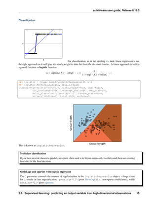
The problem solved in supervised learning
Supervised learning consists in learning the link between two datasets: the observed data X and an external
variable y that we are trying to predict, usually called “target” or “labels”. Most often, y is a 1D array of length
n_samples.
All supervised estimators in scikit-learn implement a fit(X, y) method to fit the model and a predict(X)
method that, given unlabeled observations X, returns the predicted labels y.
Vocabulary: classification and regression
If the prediction task is to classify the observations in a set of finite labels, in other words to “name” the objects
observed, the task is said to be a classification task. On the other hand, if the goal is to predict a continuous
target variable, it is said to be a regression task.
When doing classification in scikit-learn, y is a vector of integers or strings.
Note: See the Introduction to machine learning with scikit-learn Tutorial for a quick run-through on the basic
machine learning vocabulary used within scikit-learn.
2.2.1 Nearest neighbor and the curse of dimensionality
Classifying irises:
The iris dataset is a classification task
consisting in identifying 3 different types of irises (Setosa, Versicolour, and Virginica) from their petal and sepal
length and width:
>>> import numpy as np
>>> from sklearn import datasets
>>> iris = datasets.load_iris()
>>> iris_X = iris.data
>>> iris_y = iris.target
>>> np.unique(iris_y)
array([0, 1, 2])
2.2. Supervised learning: predicting an output variable from high-dimensional observations 9](https://image.slidesharecdn.com/scikit-learn0-150409112902-conversion-gate01/85/Scikit-learn-0-16-0-user-guide-19-320.jpg)
![scikit-learn user guide, Release 0.16.0
k-Nearest neighbors classifier
The simplest possible classifier is the nearest neighbor: given a new observation X_test, find in the training set (i.e.
the data used to train the estimator) the observation with the closest feature vector. (Please see the Nearest Neighbors
section of the online Scikit-learn documentation for more information about this type of classifier.)
Training set and testing set
While experimenting with any learning algorithm, it is important not to test the prediction of an estimator on the
data used to fit the estimator as this would not be evaluating the performance of the estimator on new data. This
is why datasets are often split into train and test data.
KNN (k nearest neighbors) classification example:
>>> # Split iris data in train and test data
>>> # A random permutation, to split the data randomly
>>> np.random.seed(0)
>>> indices = np.random.permutation(len(iris_X))
>>> iris_X_train = iris_X[indices[:-10]]
>>> iris_y_train = iris_y[indices[:-10]]
>>> iris_X_test = iris_X[indices[-10:]]
>>> iris_y_test = iris_y[indices[-10:]]
>>> # Create and fit a nearest-neighbor classifier
>>> from sklearn.neighbors import KNeighborsClassifier
>>> knn = KNeighborsClassifier()
>>> knn.fit(iris_X_train, iris_y_train)
KNeighborsClassifier(algorithm='auto', leaf_size=30, metric='minkowski',
metric_params=None, n_neighbors=5, p=2, weights='uniform')
>>> knn.predict(iris_X_test)
array([1, 2, 1, 0, 0, 0, 2, 1, 2, 0])
>>> iris_y_test
array([1, 1, 1, 0, 0, 0, 2, 1, 2, 0])
10 Chapter 2. A tutorial on statistical-learning for scientific data processing](https://image.slidesharecdn.com/scikit-learn0-150409112902-conversion-gate01/85/Scikit-learn-0-16-0-user-guide-20-320.jpg)
![scikit-learn user guide, Release 0.16.0
The curse of dimensionality
For an estimator to be effective, you need the distance between neighboring points to be less than some value 𝑑, which
depends on the problem. In one dimension, this requires on average 𝑛 1/𝑑 points. In the context of the above 𝑘-NN
example, if the data is described by just one feature with values ranging from 0 to 1 and with 𝑛 training observations,
then new data will be no further away than 1/𝑛. Therefore, the nearest neighbor decision rule will be efficient as soon
as 1/𝑛 is small compared to the scale of between-class feature variations.
If the number of features is 𝑝, you now require 𝑛 1/𝑑 𝑝
points. Let’s say that we require 10 points in one dimension:
now 10 𝑝
points are required in 𝑝 dimensions to pave the [0, 1] space. As 𝑝 becomes large, the number of training points
required for a good estimator grows exponentially.
For example, if each point is just a single number (8 bytes), then an effective 𝑘-NN estimator in a paltry 𝑝 20 di-
mensions would require more training data than the current estimated size of the entire internet (±1000 Exabytes or
so).
This is called the curse of dimensionality and is a core problem that machine learning addresses.
2.2.2 Linear model: from regression to sparsity
Diabetes dataset
The diabetes dataset consists of 10 physiological variables (age, sex, weight, blood pressure) measure on 442
patients, and an indication of disease progression after one year:
>>> diabetes = datasets.load_diabetes()
>>> diabetes_X_train = diabetes.data[:-20]
>>> diabetes_X_test = diabetes.data[-20:]
>>> diabetes_y_train = diabetes.target[:-20]
>>> diabetes_y_test = diabetes.target[-20:]
The task at hand is to predict disease progression from physiological variables.
Linear regression
LinearRegression, in it’s simplest form, fits a linear model to the data set by adjusting a set
of parameters in order to make the sum of the squared residuals of the model as small as possible.
Linear models: 𝑦 = 𝑋𝛽 + 𝜖
• 𝑋: data
• 𝑦: target variable
• 𝛽: Coefficients
2.2. Supervised learning: predicting an output variable from high-dimensional observations 11](https://image.slidesharecdn.com/scikit-learn0-150409112902-conversion-gate01/85/Scikit-learn-0-16-0-user-guide-21-320.jpg)
![scikit-learn user guide, Release 0.16.0
• 𝜖: Observation noise
>>> from sklearn import linear_model
>>> regr = linear_model.LinearRegression()
>>> regr.fit(diabetes_X_train, diabetes_y_train)
LinearRegression(copy_X=True, fit_intercept=True, n_jobs=1, normalize=False)
>>> print(regr.coef_)
[ 0.30349955 -237.63931533 510.53060544 327.73698041 -814.13170937
492.81458798 102.84845219 184.60648906 743.51961675 76.09517222]
>>> # The mean square error
>>> np.mean((regr.predict(diabetes_X_test)-diabetes_y_test)**2)
2004.56760268...
>>> # Explained variance score: 1 is perfect prediction
>>> # and 0 means that there is no linear relationship
>>> # between X and Y.
>>> regr.score(diabetes_X_test, diabetes_y_test)
0.5850753022690...
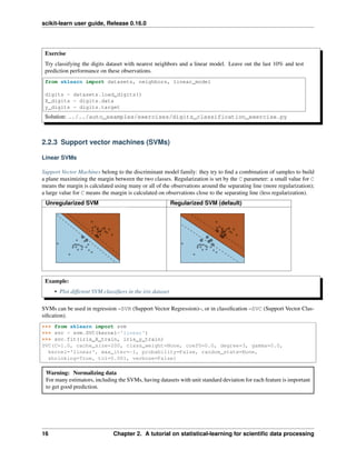
Shrinkage
If there are few data points per dimension, noise in the observations induces high variance:
>>> X = np.c_[ .5, 1].T
>>> y = [.5, 1]
>>> test = np.c_[ 0, 2].T
>>> regr = linear_model.LinearRegression()
>>> import pylab as pl
>>> pl.figure()
>>> np.random.seed(0)
>>> for _ in range(6):
... this_X = .1*np.random.normal(size=(2, 1)) + X
... regr.fit(this_X, y)
... pl.plot(test, regr.predict(test))
... pl.scatter(this_X, y, s=3)
A solution in high-dimensional statistical learning is to shrink the regression coefficients to zero: any
two randomly chosen set of observations are likely to be uncorrelated. This is called Ridge regression:
12 Chapter 2. A tutorial on statistical-learning for scientific data processing](https://image.slidesharecdn.com/scikit-learn0-150409112902-conversion-gate01/85/Scikit-learn-0-16-0-user-guide-22-320.jpg)
![scikit-learn user guide, Release 0.16.0
>>> regr = linear_model.Ridge(alpha=.1)
>>> pl.figure()
>>> np.random.seed(0)
>>> for _ in range(6):
... this_X = .1*np.random.normal(size=(2, 1)) + X
... regr.fit(this_X, y)
... pl.plot(test, regr.predict(test))
... pl.scatter(this_X, y, s=3)
This is an example of bias/variance tradeoff: the larger the ridge alpha parameter, the higher the bias and the lower
the variance.
We can choose alpha to minimize left out error, this time using the diabetes dataset rather than our synthetic data:
>>> alphas = np.logspace(-4, -1, 6)
>>> from __future__ import print_function
>>> print([regr.set_params(alpha=alpha
... ).fit(diabetes_X_train, diabetes_y_train,
... ).score(diabetes_X_test, diabetes_y_test) for alpha in alphas])
[0.5851110683883..., 0.5852073015444..., 0.5854677540698..., 0.5855512036503..., 0.5830717085554...,
Note: Capturing in the fitted parameters noise that prevents the model to generalize to new data is called overfitting.
The bias introduced by the ridge regression is called a regularization.
Sparsity
Fitting only features 1 and 2
2.2. Supervised learning: predicting an output variable from high-dimensional observations 13](https://image.slidesharecdn.com/scikit-learn0-150409112902-conversion-gate01/85/Scikit-learn-0-16-0-user-guide-23-320.jpg)
![scikit-learn user guide, Release 0.16.0
Note: A representation of the full diabetes dataset would involve 11 dimensions (10 feature dimensions and one of
the target variable). It is hard to develop an intuition on such representation, but it may be useful to keep in mind that
it would be a fairly empty space.
We can see that, although feature 2 has a strong coefficient on the full model, it conveys little information on y when
considered with feature 1.
To improve the conditioning of the problem (i.e. mitigating the The curse of dimensionality), it would be interesting
to select only the informative features and set non-informative ones, like feature 2 to 0. Ridge regression will decrease
their contribution, but not set them to zero. Another penalization approach, called Lasso (least absolute shrinkage and
selection operator), can set some coefficients to zero. Such methods are called sparse method and sparsity can be
seen as an application of Occam’s razor: prefer simpler models.
>>> regr = linear_model.Lasso()
>>> scores = [regr.set_params(alpha=alpha
... ).fit(diabetes_X_train, diabetes_y_train
... ).score(diabetes_X_test, diabetes_y_test)
... for alpha in alphas]
>>> best_alpha = alphas[scores.index(max(scores))]
>>> regr.alpha = best_alpha
>>> regr.fit(diabetes_X_train, diabetes_y_train)
Lasso(alpha=0.025118864315095794, copy_X=True, fit_intercept=True,
max_iter=1000, normalize=False, positive=False, precompute=False,
random_state=None, selection='cyclic', tol=0.0001, warm_start=False)
>>> print(regr.coef_)
[ 0. -212.43764548 517.19478111 313.77959962 -160.8303982 -0.
-187.19554705 69.38229038 508.66011217 71.84239008]
Different algorithms for the same problem
Different algorithms can be used to solve the same mathematical problem. For instance the Lasso object
in scikit-learn solves the lasso regression problem using a coordinate decent method, that is efficient on large
datasets. However, scikit-learn also provides the LassoLars object using the LARS algorthm, which is very
efficient for problems in which the weight vector estimated is very sparse (i.e. problems with very few observa-
tions).
14 Chapter 2. A tutorial on statistical-learning for scientific data processing](https://image.slidesharecdn.com/scikit-learn0-150409112902-conversion-gate01/85/Scikit-learn-0-16-0-user-guide-24-320.jpg)

![scikit-learn user guide, Release 0.16.0
Exercise
Try classifying classes 1 and 2 from the iris dataset with SVMs, with the 2 first features. Leave out 10% of each
class and test prediction performance on these observations.
Warning: the classes are ordered, do not leave out the last 10%, you would be testing on only one class.
Hint: You can use the decision_function method on a grid to get intuitions.
iris = datasets.load_iris()
X = iris.data
y = iris.target
X = X[y != 0, :2]
y = y[y != 0]
Solution: ../../auto_examples/exercises/plot_iris_exercise.py
2.3 Model selection: choosing estimators and their parameters
2.3.1 Score, and cross-validated scores
As we have seen, every estimator exposes a score method that can judge the quality of the fit (or the prediction) on
new data. Bigger is better.
>>> from sklearn import datasets, svm
>>> digits = datasets.load_digits()
>>> X_digits = digits.data
>>> y_digits = digits.target
>>> svc = svm.SVC(C=1, kernel='linear')
>>> svc.fit(X_digits[:-100], y_digits[:-100]).score(X_digits[-100:], y_digits[-100:])
0.97999999999999998
18 Chapter 2. A tutorial on statistical-learning for scientific data processing](https://image.slidesharecdn.com/scikit-learn0-150409112902-conversion-gate01/85/Scikit-learn-0-16-0-user-guide-28-320.jpg)
![scikit-learn user guide, Release 0.16.0
To get a better measure of prediction accuracy (which we can use as a proxy for goodness of fit of the model), we can
successively split the data in folds that we use for training and testing:
>>> import numpy as np
>>> X_folds = np.array_split(X_digits, 3)
>>> y_folds = np.array_split(y_digits, 3)
>>> scores = list()
>>> for k in range(3):
... # We use 'list' to copy, in order to 'pop' later on
... X_train = list(X_folds)
... X_test = X_train.pop(k)
... X_train = np.concatenate(X_train)
... y_train = list(y_folds)
... y_test = y_train.pop(k)
... y_train = np.concatenate(y_train)
... scores.append(svc.fit(X_train, y_train).score(X_test, y_test))
>>> print(scores)
[0.93489148580968284, 0.95659432387312182, 0.93989983305509184]
This is called a KFold cross validation
2.3.2 Cross-validation generators
The code above to split data in train and test sets is tedious to write. Scikit-learn exposes cross-validation generators
to generate list of indices for this purpose:
>>> from sklearn import cross_validation
>>> k_fold = cross_validation.KFold(n=6, n_folds=3)
>>> for train_indices, test_indices in k_fold:
... print('Train: %s | test: %s' % (train_indices, test_indices))
Train: [2 3 4 5] | test: [0 1]
Train: [0 1 4 5] | test: [2 3]
Train: [0 1 2 3] | test: [4 5]
The cross-validation can then be implemented easily:
>>> kfold = cross_validation.KFold(len(X_digits), n_folds=3)
>>> [svc.fit(X_digits[train], y_digits[train]).score(X_digits[test], y_digits[test])
... for train, test in kfold]
[0.93489148580968284, 0.95659432387312182, 0.93989983305509184]
To compute the score method of an estimator, the sklearn exposes a helper function:
>>> cross_validation.cross_val_score(svc, X_digits, y_digits, cv=kfold, n_jobs=-1)
array([ 0.93489149, 0.95659432, 0.93989983])
n_jobs=-1 means that the computation will be dispatched on all the CPUs of the computer.
Cross-validation generators
KFold (n, k) StratifiedKFold (y, k) LeaveOneOut
(n)
LeaveOneLabelOut
(labels)
Split it K folds, train on K-1
and then test on left-out
It preserves the class ratios / label
distribution within each fold.
Leave one
observation
out
Takes a label array to
group observations
2.3. Model selection: choosing estimators and their parameters 19](https://image.slidesharecdn.com/scikit-learn0-150409112902-conversion-gate01/85/Scikit-learn-0-16-0-user-guide-29-320.jpg)
![scikit-learn user guide, Release 0.16.0
Exercise
On the digits dataset, plot the cross-validation
score of a SVC estimator with an linear kernel as a function of parameter C (use a logarithmic grid of points,
from 1 to 10).
import numpy as np
from sklearn import cross_validation, datasets, svm
digits = datasets.load_digits()
X = digits.data
y = digits.target
svc = svm.SVC(kernel='linear')
C_s = np.logspace(-10, 0, 10)
Solution: Cross-validation on Digits Dataset Exercise
2.3.3 Grid-search and cross-validated estimators
Grid-search
The sklearn provides an object that, given data, computes the score during the fit of an estimator on a parameter
grid and chooses the parameters to maximize the cross-validation score. This object takes an estimator during the
construction and exposes an estimator API:
>>> from sklearn.grid_search import GridSearchCV
>>> Cs = np.logspace(-6, -1, 10)
>>> clf = GridSearchCV(estimator=svc, param_grid=dict(C=Cs),
... n_jobs=-1)
>>> clf.fit(X_digits[:1000], y_digits[:1000])
GridSearchCV(cv=None,...
>>> clf.best_score_
0.925...
>>> clf.best_estimator_.C
0.0077...
>>> # Prediction performance on test set is not as good as on train set
>>> clf.score(X_digits[1000:], y_digits[1000:])
0.943...
20 Chapter 2. A tutorial on statistical-learning for scientific data processing](https://image.slidesharecdn.com/scikit-learn0-150409112902-conversion-gate01/85/Scikit-learn-0-16-0-user-guide-30-320.jpg)
![scikit-learn user guide, Release 0.16.0
By default, the GridSearchCV uses a 3-fold cross-validation. However, if it detects that a classifier is passed, rather
than a regressor, it uses a stratified 3-fold.
Nested cross-validation
>>> cross_validation.cross_val_score(clf, X_digits, y_digits)
...
array([ 0.938..., 0.963..., 0.944...])
Two cross-validation loops are performed in parallel: one by the GridSearchCV estimator to set gamma and
the other one by cross_val_score to measure the prediction performance of the estimator. The resulting
scores are unbiased estimates of the prediction score on new data.
Warning: You cannot nest objects with parallel computing (n_jobs different than 1).
Cross-validated estimators
Cross-validation to set a parameter can be done more efficiently on an algorithm-by-algorithm basis. This is why for
certain estimators the sklearn exposes Cross-validation: evaluating estimator performance estimators that set their
parameter automatically by cross-validation:
>>> from sklearn import linear_model, datasets
>>> lasso = linear_model.LassoCV()
>>> diabetes = datasets.load_diabetes()
>>> X_diabetes = diabetes.data
>>> y_diabetes = diabetes.target
>>> lasso.fit(X_diabetes, y_diabetes)
LassoCV(alphas=None, copy_X=True, cv=None, eps=0.001, fit_intercept=True,
max_iter=1000, n_alphas=100, n_jobs=1, normalize=False, positive=False,
precompute='auto', random_state=None, selection='cyclic', tol=0.0001,
verbose=False)
>>> # The estimator chose automatically its lambda:
>>> lasso.alpha_
0.01229...
These estimators are called similarly to their counterparts, with ‘CV’ appended to their name.
Exercise
On the diabetes dataset, find the optimal regularization parameter alpha.
Bonus: How much can you trust the selection of alpha?
from sklearn import cross_validation, datasets, linear_model
diabetes = datasets.load_diabetes()
X = diabetes.data[:150]
y = diabetes.target[:150]
lasso = linear_model.Lasso()
alphas = np.logspace(-4, -.5, 30)
Solution: Cross-validation on diabetes Dataset Exercise
2.3. Model selection: choosing estimators and their parameters 21](https://image.slidesharecdn.com/scikit-learn0-150409112902-conversion-gate01/85/Scikit-learn-0-16-0-user-guide-31-320.jpg)
![scikit-learn user guide, Release 0.16.0
2.4 Unsupervised learning: seeking representations of the data
2.4.1 Clustering: grouping observations together
The problem solved in clustering
Given the iris dataset, if we knew that there were 3 types of iris, but did not have access to a taxonomist to label
them: we could try a clustering task: split the observations into well-separated group called clusters.
K-means clustering
Note that there exist a lot of different clustering criteria and associated algorithms. The simplest clustering algorithm
is K-means.
>>> from sklearn import cluster, datasets
>>> iris = datasets.load_iris()
>>> X_iris = iris.data
>>> y_iris = iris.target
>>> k_means = cluster.KMeans(n_clusters=3)
>>> k_means.fit(X_iris)
KMeans(copy_x=True, init='k-means++', ...
>>> print(k_means.labels_[::10])
[1 1 1 1 1 0 0 0 0 0 2 2 2 2 2]
>>> print(y_iris[::10])
[0 0 0 0 0 1 1 1 1 1 2 2 2 2 2]
Warning: There is absolutely no guarantee of recovering a ground truth. First, choosing the right number of
clusters is hard. Second, the algorithm is sensitive to initialization, and can fall into local minima, although scikit-
learn employs several tricks to mitigate this issue.
Bad initialization 8 clusters Ground truth
Don’t over-interpret clustering results
22 Chapter 2. A tutorial on statistical-learning for scientific data processing](https://image.slidesharecdn.com/scikit-learn0-150409112902-conversion-gate01/85/Scikit-learn-0-16-0-user-guide-32-320.jpg)
![scikit-learn user guide, Release 0.16.0
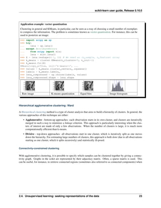
clustering an image:
from sklearn.feature_extraction.image import grid_to_graph
from sklearn.cluster import AgglomerativeClustering
###############################################################################
# Generate data
lena = sp.misc.lena()
# Downsample the image by a factor of 4
lena = lena[::2, ::2] + lena[1::2, ::2] + lena[::2, 1::2] + lena[1::2, 1::2]
X = np.reshape(lena, (-1, 1))
###############################################################################
# Define the structure A of the data. Pixels connected to their neighbors.
connectivity = grid_to_graph(*lena.shape)
###############################################################################
# Compute clustering
print("Compute structured hierarchical clustering...")
st = time.time()
n_clusters = 15 # number of regions
ward = AgglomerativeClustering(n_clusters=n_clusters,
linkage='ward', connectivity=connectivity).fit(X)
label = np.reshape(ward.labels_, lena.shape)
print("Elapsed time: ", time.time() - st)
print("Number of pixels: ", label.size)
print("Number of clusters: ", np.unique(label).size)
Feature agglomeration
We have seen that sparsity could be used to mitigate the curse of dimensionality, i.e an insufficient amount of ob-
servations compared to the number of features. Another approach is to merge together similar features: feature
agglomeration. This approach can be implemented by clustering in the feature direction, in other words clustering
24 Chapter 2. A tutorial on statistical-learning for scientific data processing](https://image.slidesharecdn.com/scikit-learn0-150409112902-conversion-gate01/85/Scikit-learn-0-16-0-user-guide-34-320.jpg)
![scikit-learn user guide, Release 0.16.0
the transposed data.
>>> digits = datasets.load_digits()
>>> images = digits.images
>>> X = np.reshape(images, (len(images), -1))
>>> connectivity = grid_to_graph(*images[0].shape)
>>> agglo = cluster.FeatureAgglomeration(connectivity=connectivity,
... n_clusters=32)
>>> agglo.fit(X)
FeatureAgglomeration(affinity='euclidean', compute_full_tree='auto',...
>>> X_reduced = agglo.transform(X)
>>> X_approx = agglo.inverse_transform(X_reduced)
>>> images_approx = np.reshape(X_approx, images.shape)
transform and inverse_transform methods
Some estimators expose a transform method, for instance to reduce the dimensionality of the dataset.
2.4.2 Decompositions: from a signal to components and loadings
Components and loadings
If X is our multivariate data, then the problem that we are trying to solve is to rewrite it on a different observa-
tional basis: we want to learn loadings L and a set of components C such that X = L C. Different criteria exist to
choose the components
Principal component analysis: PCA
Principal component analysis (PCA) selects the successive components that explain the maximum variance in the
signal.
2.4. Unsupervised learning: seeking representations of the data 25](https://image.slidesharecdn.com/scikit-learn0-150409112902-conversion-gate01/85/Scikit-learn-0-16-0-user-guide-35-320.jpg)
![scikit-learn user guide, Release 0.16.0
The point cloud spanned by the observations above is very flat in one direction: one of the three univariate features
can almost be exactly computed using the other two. PCA finds the directions in which the data is not flat
When used to transform data, PCA can reduce the dimensionality of the data by projecting on a principal subspace.
>>> # Create a signal with only 2 useful dimensions
>>> x1 = np.random.normal(size=100)
>>> x2 = np.random.normal(size=100)
>>> x3 = x1 + x2
>>> X = np.c_[x1, x2, x3]
>>> from sklearn import decomposition
>>> pca = decomposition.PCA()
>>> pca.fit(X)
PCA(copy=True, n_components=None, whiten=False)
>>> print(pca.explained_variance_)
[ 2.18565811e+00 1.19346747e+00 8.43026679e-32]
>>> # As we can see, only the 2 first components are useful
>>> pca.n_components = 2
>>> X_reduced = pca.fit_transform(X)
>>> X_reduced.shape
(100, 2)
Independent Component Analysis: ICA
Independent component analysis (ICA) selects components so that the distribution of their loadings carries
a maximum amount of independent information. It is able to recover non-Gaussian independent signals:
26 Chapter 2. A tutorial on statistical-learning for scientific data processing](https://image.slidesharecdn.com/scikit-learn0-150409112902-conversion-gate01/85/Scikit-learn-0-16-0-user-guide-36-320.jpg)
![scikit-learn user guide, Release 0.16.0
>>> # Generate sample data
>>> time = np.linspace(0, 10, 2000)
>>> s1 = np.sin(2 * time) # Signal 1 : sinusoidal signal
>>> s2 = np.sign(np.sin(3 * time)) # Signal 2 : square signal
>>> S = np.c_[s1, s2]
>>> S += 0.2 * np.random.normal(size=S.shape) # Add noise
>>> S /= S.std(axis=0) # Standardize data
>>> # Mix data
>>> A = np.array([[1, 1], [0.5, 2]]) # Mixing matrix
>>> X = np.dot(S, A.T) # Generate observations
>>> # Compute ICA
>>> ica = decomposition.FastICA()
>>> S_ = ica.fit_transform(X) # Get the estimated sources
>>> A_ = ica.mixing_.T
>>> np.allclose(X, np.dot(S_, A_) + ica.mean_)
True
2.4. Unsupervised learning: seeking representations of the data 27](https://image.slidesharecdn.com/scikit-learn0-150409112902-conversion-gate01/85/Scikit-learn-0-16-0-user-guide-37-320.jpg)
![scikit-learn user guide, Release 0.16.0
2.5 Putting it all together
2.5.1 Pipelining
We have seen that some estimators can transform data and that some estimators can predict variables. We can also
create combined estimators:
from sklearn import linear_model, decomposition, datasets
from sklearn.pipeline import Pipeline
from sklearn.grid_search import GridSearchCV
logistic = linear_model.LogisticRegression()
pca = decomposition.PCA()
pipe = Pipeline(steps=[('pca', pca), ('logistic', logistic)])
digits = datasets.load_digits()
X_digits = digits.data
y_digits = digits.target
###############################################################################
# Plot the PCA spectrum
pca.fit(X_digits)
plt.figure(1, figsize=(4, 3))
plt.clf()
plt.axes([.2, .2, .7, .7])
plt.plot(pca.explained_variance_, linewidth=2)
plt.axis('tight')
plt.xlabel('n_components')
plt.ylabel('explained_variance_')
###############################################################################
# Prediction
n_components = [20, 40, 64]
Cs = np.logspace(-4, 4, 3)
#Parameters of pipelines can be set using ‘__’ separated parameter names:
estimator = GridSearchCV(pipe,
dict(pca__n_components=n_components,
logistic__C=Cs))
estimator.fit(X_digits, y_digits)
28 Chapter 2. A tutorial on statistical-learning for scientific data processing](https://image.slidesharecdn.com/scikit-learn0-150409112902-conversion-gate01/85/Scikit-learn-0-16-0-user-guide-38-320.jpg)
![scikit-learn user guide, Release 0.16.0
plt.axvline(estimator.best_estimator_.named_steps['pca'].n_components,
linestyle=':', label='n_components chosen')
plt.legend(prop=dict(size=12))
2.5.2 Face recognition with eigenfaces
The dataset used in this example is a preprocessed excerpt of the “Labeled Faces in the Wild”, also known as LFW:
http://vis-www.cs.umass.edu/lfw/lfw-funneled.tgz (233MB)
"""
===================================================
Faces recognition example using eigenfaces and SVMs
===================================================
The dataset used in this example is a preprocessed excerpt of the
"Labeled Faces in the Wild", aka LFW_:
http://vis-www.cs.umass.edu/lfw/lfw-funneled.tgz (233MB)
.. _LFW: http://vis-www.cs.umass.edu/lfw/
Expected results for the top 5 most represented people in the dataset::
precision recall f1-score support
Gerhard_Schroeder 0.91 0.75 0.82 28
Donald_Rumsfeld 0.84 0.82 0.83 33
Tony_Blair 0.65 0.82 0.73 34
Colin_Powell 0.78 0.88 0.83 58
George_W_Bush 0.93 0.86 0.90 129
avg / total 0.86 0.84 0.85 282
"""
from __future__ import print_function
from time import time
import logging
import matplotlib.pyplot as plt
from sklearn.cross_validation import train_test_split
from sklearn.datasets import fetch_lfw_people
from sklearn.grid_search import GridSearchCV
from sklearn.metrics import classification_report
from sklearn.metrics import confusion_matrix
from sklearn.decomposition import RandomizedPCA
from sklearn.svm import SVC
print(__doc__)
# Display progress logs on stdout
logging.basicConfig(level=logging.INFO, format='%(asctime)s %(message)s')
2.5. Putting it all together 29](https://image.slidesharecdn.com/scikit-learn0-150409112902-conversion-gate01/85/Scikit-learn-0-16-0-user-guide-39-320.jpg)
![scikit-learn user guide, Release 0.16.0
###############################################################################
# Download the data, if not already on disk and load it as numpy arrays
lfw_people = fetch_lfw_people(min_faces_per_person=70, resize=0.4)
# introspect the images arrays to find the shapes (for plotting)
n_samples, h, w = lfw_people.images.shape
# for machine learning we use the 2 data directly (as relative pixel
# positions info is ignored by this model)
X = lfw_people.data
n_features = X.shape[1]
# the label to predict is the id of the person
y = lfw_people.target
target_names = lfw_people.target_names
n_classes = target_names.shape[0]
print("Total dataset size:")
print("n_samples: %d" % n_samples)
print("n_features: %d" % n_features)
print("n_classes: %d" % n_classes)
###############################################################################
# Split into a training set and a test set using a stratified k fold
# split into a training and testing set
X_train, X_test, y_train, y_test = train_test_split(
X, y, test_size=0.25)
###############################################################################
# Compute a PCA (eigenfaces) on the face dataset (treated as unlabeled
# dataset): unsupervised feature extraction / dimensionality reduction
n_components = 150
print("Extracting the top %d eigenfaces from %d faces"
% (n_components, X_train.shape[0]))
t0 = time()
pca = RandomizedPCA(n_components=n_components, whiten=True).fit(X_train)
print("done in %0.3fs" % (time() - t0))
eigenfaces = pca.components_.reshape((n_components, h, w))
print("Projecting the input data on the eigenfaces orthonormal basis")
t0 = time()
X_train_pca = pca.transform(X_train)
X_test_pca = pca.transform(X_test)
print("done in %0.3fs" % (time() - t0))
###############################################################################
# Train a SVM classification model
print("Fitting the classifier to the training set")
t0 = time()
param_grid = {'C': [1e3, 5e3, 1e4, 5e4, 1e5],
30 Chapter 2. A tutorial on statistical-learning for scientific data processing](https://image.slidesharecdn.com/scikit-learn0-150409112902-conversion-gate01/85/Scikit-learn-0-16-0-user-guide-40-320.jpg)
![scikit-learn user guide, Release 0.16.0
'gamma': [0.0001, 0.0005, 0.001, 0.005, 0.01, 0.1], }
clf = GridSearchCV(SVC(kernel='rbf', class_weight='auto'), param_grid)
clf = clf.fit(X_train_pca, y_train)
print("done in %0.3fs" % (time() - t0))
print("Best estimator found by grid search:")
print(clf.best_estimator_)
###############################################################################
# Quantitative evaluation of the model quality on the test set
print("Predicting people's names on the test set")
t0 = time()
y_pred = clf.predict(X_test_pca)
print("done in %0.3fs" % (time() - t0))
print(classification_report(y_test, y_pred, target_names=target_names))
print(confusion_matrix(y_test, y_pred, labels=range(n_classes)))
###############################################################################
# Qualitative evaluation of the predictions using matplotlib
def plot_gallery(images, titles, h, w, n_row=3, n_col=4):
"""Helper function to plot a gallery of portraits"""
plt.figure(figsize=(1.8 * n_col, 2.4 * n_row))
plt.subplots_adjust(bottom=0, left=.01, right=.99, top=.90, hspace=.35)
for i in range(n_row * n_col):
plt.subplot(n_row, n_col, i + 1)
plt.imshow(images[i].reshape((h, w)), cmap=plt.cm.gray)
plt.title(titles[i], size=12)
plt.xticks(())
plt.yticks(())
# plot the result of the prediction on a portion of the test set
def title(y_pred, y_test, target_names, i):
pred_name = target_names[y_pred[i]].rsplit(' ', 1)[-1]
true_name = target_names[y_test[i]].rsplit(' ', 1)[-1]
return 'predicted: %sntrue: %s' % (pred_name, true_name)
prediction_titles = [title(y_pred, y_test, target_names, i)
for i in range(y_pred.shape[0])]
plot_gallery(X_test, prediction_titles, h, w)
# plot the gallery of the most significative eigenfaces
eigenface_titles = ["eigenface %d" % i for i in range(eigenfaces.shape[0])]
plot_gallery(eigenfaces, eigenface_titles, h, w)
plt.show()
2.5. Putting it all together 31](https://image.slidesharecdn.com/scikit-learn0-150409112902-conversion-gate01/85/Scikit-learn-0-16-0-user-guide-41-320.jpg)


![scikit-learn user guide, Release 0.16.0
3.2 Loading the 20 newsgroups dataset
The dataset is called “Twenty Newsgroups”. Here is the official description, quoted from the website:
The 20 Newsgroups data set is a collection of approximately 20,000 newsgroup documents, partitioned
(nearly) evenly across 20 different newsgroups. To the best of our knowledge, it was originally collected
by Ken Lang, probably for his paper “Newsweeder: Learning to filter netnews,” though he does not explic-
itly mention this collection. The 20 newsgroups collection has become a popular data set for experiments
in text applications of machine learning techniques, such as text classification and text clustering.
In the following we will use the built-in dataset loader for 20 newsgroups from scikit-learn. Alternatively, it is possible
to download the dataset manually from the web-site and use the sklearn.datasets.load_files function by
pointing it to the 20news-bydate-train subfolder of the uncompressed archive folder.
In order to get faster execution times for this first example we will work on a partial dataset with only 4 categories out
of the 20 available in the dataset:
>>> categories = ['alt.atheism', 'soc.religion.christian',
... 'comp.graphics', 'sci.med']
We can now load the list of files matching those categories as follows:
>>> from sklearn.datasets import fetch_20newsgroups
>>> twenty_train = fetch_20newsgroups(subset='train',
... categories=categories, shuffle=True, random_state=42)
The returned dataset is a scikit-learn “bunch”: a simple holder object with fields that can be both accessed
as python dict keys or object attributes for convenience, for instance the target_names holds the list of the
requested category names:
>>> twenty_train.target_names
['alt.atheism', 'comp.graphics', 'sci.med', 'soc.religion.christian']
The files themselves are loaded in memory in the data attribute. For reference the filenames are also available:
>>> len(twenty_train.data)
2257
>>> len(twenty_train.filenames)
2257
Let’s print the first lines of the first loaded file:
>>> print("n".join(twenty_train.data[0].split("n")[:3]))
From: sd345@city.ac.uk (Michael Collier)
Subject: Converting images to HP LaserJet III?
Nntp-Posting-Host: hampton
>>> print(twenty_train.target_names[twenty_train.target[0]])
comp.graphics
Supervised learning algorithms will require a category label for each document in the training set. In this case the cat-
egory is the name of the newsgroup which also happens to be the name of the folder holding the individual documents.
For speed and space efficiency reasons scikit-learn loads the target attribute as an array of integers that corre-
sponds to the index of the category name in the target_names list. The category integer id of each sample is stored
in the target attribute:
>>> twenty_train.target[:10]
array([1, 1, 3, 3, 3, 3, 3, 2, 2, 2])
36 Chapter 3. Working With Text Data](https://image.slidesharecdn.com/scikit-learn0-150409112902-conversion-gate01/85/Scikit-learn-0-16-0-user-guide-46-320.jpg)
![scikit-learn user guide, Release 0.16.0
It is possible to get back the category names as follows:
>>> for t in twenty_train.target[:10]:
... print(twenty_train.target_names[t])
...
comp.graphics
comp.graphics
soc.religion.christian
soc.religion.christian
soc.religion.christian
soc.religion.christian
soc.religion.christian
sci.med
sci.med
sci.med
You can notice that the samples have been shuffled randomly (with a fixed RNG seed): this is useful if you select only
the first samples to quickly train a model and get a first idea of the results before re-training on the complete dataset
later.
3.3 Extracting features from text files
In order to perform machine learning on text documents, we first need to turn the text content into numerical feature
vectors.
3.3.1 Bags of words
The most intuitive way to do so is the bags of words representation:
1. assign a fixed integer id to each word occurring in any document of the training set (for instance by building a
dictionary from words to integer indices).
2. for each document #i, count the number of occurrences of each word w and store it in X[i, j] as the value
of feature #j where j is the index of word w in the dictionary
The bags of words representation implies that n_features is the number of distinct words in the corpus: this
number is typically larger that 100,000.
If n_samples == 10000, storing X as a numpy array of type float32 would require 10000 x 100000 x 4 bytes =
4GB in RAM which is barely manageable on today’s computers.
Fortunately, most values in X will be zeros since for a given document less than a couple thousands of distinct words
will be used. For this reason we say that bags of words are typically high-dimensional sparse datasets. We can save
a lot of memory by only storing the non-zero parts of the feature vectors in memory.
scipy.sparse matrices are data structures that do exactly this, and scikit-learn has built-in support for these
structures.
3.3.2 Tokenizing text with scikit-learn
Text preprocessing, tokenizing and filtering of stopwords are included in a high level component that is able to build a
dictionary of features and transform documents to feature vectors:
3.3. Extracting features from text files 37](https://image.slidesharecdn.com/scikit-learn0-150409112902-conversion-gate01/85/Scikit-learn-0-16-0-user-guide-47-320.jpg)

![scikit-learn user guide, Release 0.16.0
>>> docs_new = ['God is love', 'OpenGL on the GPU is fast']
>>> X_new_counts = count_vect.transform(docs_new)
>>> X_new_tfidf = tfidf_transformer.transform(X_new_counts)
>>> predicted = clf.predict(X_new_tfidf)
>>> for doc, category in zip(docs_new, predicted):
... print('%r => %s' % (doc, twenty_train.target_names[category]))
...
'God is love' => soc.religion.christian
'OpenGL on the GPU is fast' => comp.graphics
3.5 Building a pipeline
In order to make the vectorizer => transformer => classifier easier to work with, scikit-learn provides a
Pipeline class that behaves like a compound classifier:
>>> from sklearn.pipeline import Pipeline
>>> text_clf = Pipeline([('vect', CountVectorizer()),
... ('tfidf', TfidfTransformer()),
... ('clf', MultinomialNB()),
... ])
The names vect, tfidf and clf (classifier) are arbitrary. We shall see their use in the section on grid search, below.
We can now train the model with a single command:
>>> text_clf = text_clf.fit(twenty_train.data, twenty_train.target)
3.6 Evaluation of the performance on the test set
Evaluating the predictive accuracy of the model is equally easy:
>>> import numpy as np
>>> twenty_test = fetch_20newsgroups(subset='test',
... categories=categories, shuffle=True, random_state=42)
>>> docs_test = twenty_test.data
>>> predicted = text_clf.predict(docs_test)
>>> np.mean(predicted == twenty_test.target)
0.834...
I.e., we achieved 83.4% accuracy. Let’s see if we can do better with a linear support vector machine (SVM), which is
widely regarded as one of the best text classification algorithms (although it’s also a bit slower than naïve Bayes). We
can change the learner by just plugging a different classifier object into our pipeline:
>>> from sklearn.linear_model import SGDClassifier
>>> text_clf = Pipeline([('vect', CountVectorizer()),
... ('tfidf', TfidfTransformer()),
... ('clf', SGDClassifier(loss='hinge', penalty='l2',
... alpha=1e-3, n_iter=5, random_state=42)),
... ])
>>> _ = text_clf.fit(twenty_train.data, twenty_train.target)
>>> predicted = text_clf.predict(docs_test)
>>> np.mean(predicted == twenty_test.target)
0.912...
3.5. Building a pipeline 39](https://image.slidesharecdn.com/scikit-learn0-150409112902-conversion-gate01/85/Scikit-learn-0-16-0-user-guide-49-320.jpg)
![scikit-learn user guide, Release 0.16.0
scikit-learn further provides utilities for more detailed performance analysis of the results:
>>> from sklearn import metrics
>>> print(metrics.classification_report(twenty_test.target, predicted,
... target_names=twenty_test.target_names))
...
precision recall f1-score support
alt.atheism 0.95 0.81 0.87 319
comp.graphics 0.88 0.97 0.92 389
sci.med 0.94 0.90 0.92 396
soc.religion.christian 0.90 0.95 0.93 398
avg / total 0.92 0.91 0.91 1502
>>> metrics.confusion_matrix(twenty_test.target, predicted)
array([[258, 11, 15, 35],
[ 4, 379, 3, 3],
[ 5, 33, 355, 3],
[ 5, 10, 4, 379]])
As expected the confusion matrix shows that posts from the newsgroups on atheism and christian are more often
confused for one another than with computer graphics.
3.7 Parameter tuning using grid search
We’ve already encountered some parameters such as use_idf in the TfidfTransformer. Classifiers tend to have
many parameters as well; e.g., MultinomialNB includes a smoothing parameter alpha and SGDClassifier
has a penalty parameter alpha and configurable loss and penalty terms in the objective function (see the module
documentation, or use the Python help function, to get a description of these).
Instead of tweaking the parameters of the various components of the chain, it is possible to run an exhaustive search of
the best parameters on a grid of possible values. We try out all classifiers on either words or bigrams, with or without
idf, and with a penalty parameter of either 0.01 or 0.001 for the linear SVM:
>>> from sklearn.grid_search import GridSearchCV
>>> parameters = {'vect__ngram_range': [(1, 1), (1, 2)],
... 'tfidf__use_idf': (True, False),
... 'clf__alpha': (1e-2, 1e-3),
... }
Obviously, such an exhaustive search can be expensive. If we have multiple CPU cores at our disposal, we can tell
the grid searcher to try these eight parameter combinations in parallel with the n_jobs parameter. If we give this
parameter a value of -1, grid search will detect how many cores are installed and uses them all:
>>> gs_clf = GridSearchCV(text_clf, parameters, n_jobs=-1)
The grid search instance behaves like a normal scikit-learn model. Let’s perform the search on a smaller subset
of the training data to speed up the computation:
>>> gs_clf = gs_clf.fit(twenty_train.data[:400], twenty_train.target[:400])
The result of calling fit on a GridSearchCV object is a classifier that we can use to predict:
>>> twenty_train.target_names[gs_clf.predict(['God is love'])]
'soc.religion.christian'
40 Chapter 3. Working With Text Data](https://image.slidesharecdn.com/scikit-learn0-150409112902-conversion-gate01/85/Scikit-learn-0-16-0-user-guide-50-320.jpg)
![scikit-learn user guide, Release 0.16.0
but otherwise, it’s a pretty large and clumsy object. We can, however, get the optimal parameters out by inspecting the
object’s grid_scores_ attribute, which is a list of parameters/score pairs. To get the best scoring attributes, we can
do:
>>> best_parameters, score, _ = max(gs_clf.grid_scores_, key=lambda x: x[1])
>>> for param_name in sorted(parameters.keys()):
... print("%s: %r" % (param_name, best_parameters[param_name]))
...
clf__alpha: 0.001
tfidf__use_idf: True
vect__ngram_range: (1, 1)
>>> score
0.900...
3.7.1 Exercises
To do the exercises, copy the content of the ‘skeletons’ folder as a new folder named ‘workspace’:
% cp -r skeletons workspace
You can then edit the content of the workspace without fear of loosing the original exercise instructions.
Then fire an ipython shell and run the work-in-progress script with:
[1] %run workspace/exercise_XX_script.py arg1 arg2 arg3
If an exception is triggered, use %debug to fire-up a post mortem ipdb session.
Refine the implementation and iterate until the exercise is solved.
For each exercise, the skeleton file provides all the necessary import statements, boilerplate code to load the
data and sample code to evaluate the predictive accurracy of the model.
3.8 Exercise 1: Language identification
• Write a text classification pipeline using a custom preprocessor and CharNGramAnalyzer using data from
Wikipedia articles as training set.
• Evaluate the performance on some held out test set.
ipython command line:
%run workspace/exercise_01_language_train_model.py data/languages/paragraphs/
3.9 Exercise 2: Sentiment Analysis on movie reviews
• Write a text classification pipeline to classify movie reviews as either positive or negative.
• Find a good set of parameters using grid search.
• Evaluate the performance on a held out test set.
ipython command line:
3.8. Exercise 1: Language identification 41](https://image.slidesharecdn.com/scikit-learn0-150409112902-conversion-gate01/85/Scikit-learn-0-16-0-user-guide-51-320.jpg)

![scikit-learn user guide, Release 0.16.0
>>> from sklearn import linear_model
>>> clf = linear_model.LinearRegression()
>>> clf.fit ([[0, 0], [1, 1], [2, 2]], [0, 1, 2])
LinearRegression(copy_X=True, fit_intercept=True, n_jobs=1, normalize=False)
>>> clf.coef_
array([ 0.5, 0.5])
However, coefficient estimates for Ordinary Least Squares rely on the independence of the model terms. When terms
are correlated and the columns of the design matrix 𝑋 have an approximate linear dependence, the design matrix
becomes close to singular and as a result, the least-squares estimate becomes highly sensitive to random errors in the
observed response, producing a large variance. This situation of multicollinearity can arise, for example, when data
are collected without an experimental design.
Examples:
• Linear Regression Example
Ordinary Least Squares Complexity
This method computes the least squares solution using a singular value decomposition of X. If X is a matrix of size (n,
p) this method has a cost of 𝑂(𝑛𝑝2
), assuming that 𝑛 ≥ 𝑝.
4.1.2 Ridge Regression
Ridge regression addresses some of the problems of Ordinary Least Squares by imposing a penalty on the size of
coefficients. The ridge coefficients minimize a penalized residual sum of squares,
𝑚𝑖𝑛
𝑤
||𝑋𝑤 − 𝑦||2
2
+ 𝛼||𝑤||2
2
Here, 𝛼 ≥ 0 is a complexity parameter that controls the amount of shrinkage: the larger the value of 𝛼, the greater the
amount of shrinkage and thus the coefficients become more robust to collinearity.
As with other linear models, Ridge will take in its fit method arrays X, y and will store the coefficients 𝑤 of the
linear model in its coef_ member:
44 Chapter 4. Supervised learning](https://image.slidesharecdn.com/scikit-learn0-150409112902-conversion-gate01/85/Scikit-learn-0-16-0-user-guide-54-320.jpg)
![scikit-learn user guide, Release 0.16.0
>>> from sklearn import linear_model
>>> clf = linear_model.Ridge (alpha = .5)
>>> clf.fit ([[0, 0], [0, 0], [1, 1]], [0, .1, 1])
Ridge(alpha=0.5, copy_X=True, fit_intercept=True, max_iter=None,
normalize=False, solver='auto', tol=0.001)
>>> clf.coef_
array([ 0.34545455, 0.34545455])
>>> clf.intercept_
0.13636...
Examples:
• Plot Ridge coefficients as a function of the regularization
• Classification of text documents using sparse features
Ridge Complexity
This method has the same order of complexity than an Ordinary Least Squares.
Setting the regularization parameter: generalized Cross-Validation
RidgeCV implements ridge regression with built-in cross-validation of the alpha parameter. The object works in
the same way as GridSearchCV except that it defaults to Generalized Cross-Validation (GCV), an efficient form of
leave-one-out cross-validation:
>>> from sklearn import linear_model
>>> clf = linear_model.RidgeCV(alphas=[0.1, 1.0, 10.0])
>>> clf.fit([[0, 0], [0, 0], [1, 1]], [0, .1, 1])
RidgeCV(alphas=[0.1, 1.0, 10.0], cv=None, fit_intercept=True, scoring=None,
normalize=False)
>>> clf.alpha_
0.1
References
• “Notes on Regularized Least Squares”, Rifkin & Lippert (technical report, course slides).
4.1.3 Lasso
The Lasso is a linear model that estimates sparse coefficients. It is useful in some contexts due to its tendency
to prefer solutions with fewer parameter values, effectively reducing the number of variables upon which the given
solution is dependent. For this reason, the Lasso and its variants are fundamental to the field of compressed sensing.
Under certain conditions, it can recover the exact set of non-zero weights (see Compressive sensing: tomography
reconstruction with L1 prior (Lasso)).
Mathematically, it consists of a linear model trained with ℓ1 prior as regularizer. The objective function to minimize
is:
𝑚𝑖𝑛
𝑤
1
2𝑛 𝑠𝑎𝑚𝑝𝑙𝑒𝑠
||𝑋𝑤 − 𝑦||2
2 + 𝛼||𝑤||1
4.1. Generalized Linear Models 45](https://image.slidesharecdn.com/scikit-learn0-150409112902-conversion-gate01/85/Scikit-learn-0-16-0-user-guide-55-320.jpg)
![scikit-learn user guide, Release 0.16.0
The lasso estimate thus solves the minimization of the least-squares penalty with 𝛼||𝑤||1 added, where 𝛼 is a constant
and ||𝑤||1 is the ℓ1-norm of the parameter vector.
The implementation in the class Lasso uses coordinate descent as the algorithm to fit the coefficients. See Least
Angle Regression for another implementation:
>>> clf = linear_model.Lasso(alpha = 0.1)
>>> clf.fit([[0, 0], [1, 1]], [0, 1])
Lasso(alpha=0.1, copy_X=True, fit_intercept=True, max_iter=1000,
normalize=False, positive=False, precompute=False, random_state=None,
selection='cyclic', tol=0.0001, warm_start=False)
>>> clf.predict([[1, 1]])
array([ 0.8])
Also useful for lower-level tasks is the function lasso_path that computes the coefficients along the full path of
possible values.
Examples:
• Lasso and Elastic Net for Sparse Signals
• Compressive sensing: tomography reconstruction with L1 prior (Lasso)
Note: Feature selection with Lasso
As the Lasso regression yields sparse models, it can thus be used to perform feature selection, as detailed in L1-based
feature selection.
Note: Randomized sparsity
For feature selection or sparse recovery, it may be interesting to use Randomized sparse models.
Setting regularization parameter
The alpha parameter controls the degree of sparsity of the coefficients estimated.
Using cross-validation
scikit-learn exposes objects that set the Lasso alpha parameter by cross-validation: LassoCV and LassoLarsCV.
LassoLarsCV is based on the Least Angle Regression algorithm explained below.
For high-dimensional datasets with many collinear regressors, LassoCV is most often preferable. However,
LassoLarsCV has the advantage of exploring more relevant values of alpha parameter, and if the number of samples
is very small compared to the number of observations, it is often faster than LassoCV.
46 Chapter 4. Supervised learning](https://image.slidesharecdn.com/scikit-learn0-150409112902-conversion-gate01/85/Scikit-learn-0-16-0-user-guide-56-320.jpg)

![scikit-learn user guide, Release 0.16.0
• Because LARS is based upon an iterative refitting of the residuals, it would appear to be especially sensitive to
the effects of noise. This problem is discussed in detail by Weisberg in the discussion section of the Efron et al.
(2004) Annals of Statistics article.
The LARS model can be used using estimator Lars, or its low-level implementation lars_path.
4.1.7 LARS Lasso
LassoLars is a lasso model implemented using the LARS algorithm, and unlike the implementation based on
coordinate_descent, this yields the exact solution, which is piecewise linear as a function of the norm of its coefficients.
>>> from sklearn import linear_model
>>> clf = linear_model.LassoLars(alpha=.1)
>>> clf.fit([[0, 0], [1, 1]], [0, 1])
LassoLars(alpha=0.1, copy_X=True, eps=..., fit_intercept=True,
fit_path=True, max_iter=500, normalize=True, precompute='auto',
verbose=False)
>>> clf.coef_
array([ 0.717157..., 0. ])
Examples:
• Lasso path using LARS
The Lars algorithm provides the full path of the coefficients along the regularization parameter almost for free, thus a
common operation consist of retrieving the path with function lars_path
Mathematical formulation
The algorithm is similar to forward stepwise regression, but instead of including variables at each step, the estimated
parameters are increased in a direction equiangular to each one’s correlations with the residual.
Instead of giving a vector result, the LARS solution consists of a curve denoting the solution for each value of the
L1 norm of the parameter vector. The full coefficients path is stored in the array coef_path_, which has size
(n_features, max_features+1). The first column is always zero.
50 Chapter 4. Supervised learning](https://image.slidesharecdn.com/scikit-learn0-150409112902-conversion-gate01/85/Scikit-learn-0-16-0-user-guide-60-320.jpg)

![scikit-learn user guide, Release 0.16.0
The disadvantages of Bayesian regression include:
• Inference of the model can be time consuming.
References
• A good introduction to Bayesian methods is given in C. Bishop: Pattern Recognition and Machine learning
• Original Algorithm is detailed in the book Bayesian learning for neural networks by Radford M. Neal
Bayesian Ridge Regression
BayesianRidge estimates a probabilistic model of the regression problem as described above. The prior for the
parameter 𝑤 is given by a spherical Gaussian:
𝑝(𝑤|𝜆) = 𝒩(𝑤|0, 𝜆−1
Ip)
The priors over 𝛼 and 𝜆 are chosen to be gamma distributions, the conjugate prior for the precision of the Gaussian.
The resulting model is called Bayesian Ridge Regression, and is similar to the classical Ridge. The parameters
𝑤, 𝛼 and 𝜆 are estimated jointly during the fit of the model. The remaining hyperparameters are the parameters of
the gamma priors over 𝛼 and 𝜆. These are usually chosen to be non-informative. The parameters are estimated by
maximizing the marginal log likelihood.
By default 𝛼1 = 𝛼2 = 𝜆1 = 𝜆2 = 1.𝑒−6
.
Bayesian Ridge Regression is used for regression:
>>> from sklearn import linear_model
>>> X = [[0., 0.], [1., 1.], [2., 2.], [3., 3.]]
>>> Y = [0., 1., 2., 3.]
>>> clf = linear_model.BayesianRidge()
>>> clf.fit(X, Y)
BayesianRidge(alpha_1=1e-06, alpha_2=1e-06, compute_score=False, copy_X=True,
fit_intercept=True, lambda_1=1e-06, lambda_2=1e-06, n_iter=300,
normalize=False, tol=0.001, verbose=False)
After being fitted, the model can then be used to predict new values:
52 Chapter 4. Supervised learning](https://image.slidesharecdn.com/scikit-learn0-150409112902-conversion-gate01/85/Scikit-learn-0-16-0-user-guide-62-320.jpg)
![scikit-learn user guide, Release 0.16.0
>>> clf.predict ([[1, 0.]])
array([ 0.50000013])
The weights 𝑤 of the model can be access:
>>> clf.coef_
array([ 0.49999993, 0.49999993])
Due to the Bayesian framework, the weights found are slightly different to the ones found by Ordinary Least Squares.
However, Bayesian Ridge Regression is more robust to ill-posed problem.
Examples:
• Bayesian Ridge Regression
References
• More details can be found in the article Bayesian Interpolation by MacKay, David J. C.
Automatic Relevance Determination - ARD
ARDRegression is very similar to Bayesian Ridge Regression, but can lead to sparser weights 𝑤 1 2
.
ARDRegression poses a different prior over 𝑤, by dropping the assumption of the Gaussian being spherical.
Instead, the distribution over 𝑤 is assumed to be an axis-parallel, elliptical Gaussian distribution.
This means each weight 𝑤𝑖 is drawn from a Gaussian distribution, centered on zero and with a precision 𝜆𝑖:
𝑝(𝑤|𝜆) = 𝒩(𝑤|0, 𝐴−1
)
with 𝑑𝑖𝑎𝑔 (𝐴) = 𝜆 = {𝜆1, ..., 𝜆 𝑝}.
In contrast to Bayesian Ridge Regression, each coordinate of 𝑤𝑖 has its own standard deviation 𝜆𝑖. The prior over all
𝜆𝑖 is chosen to be the same gamma distribution given by hyperparameters 𝜆1 and 𝜆2.
1 Christopher M. Bishop: Pattern Recognition and Machine Learning, Chapter 7.2.1
2 David Wipf and Srikantan Nagarajan: A new view of automatic relevance determination.
4.1. Generalized Linear Models 53](https://image.slidesharecdn.com/scikit-learn0-150409112902-conversion-gate01/85/Scikit-learn-0-16-0-user-guide-63-320.jpg)


![scikit-learn user guide, Release 0.16.0
For example, a simple linear regression can be extended by constructing polynomial features from the coefficients.
In the standard linear regression case, you might have a model that looks like this for two-dimensional data:
ˆ𝑦(𝑤, 𝑥) = 𝑤0 + 𝑤1 𝑥1 + 𝑤2 𝑥2
If we want to fit a paraboloid to the data instead of a plane, we can combine the features in second-order polynomials,
so that the model looks like this:
ˆ𝑦(𝑤, 𝑥) = 𝑤0 + 𝑤1 𝑥1 + 𝑤2 𝑥2 + 𝑤3 𝑥1 𝑥2 + 𝑤4 𝑥2
1 + 𝑤5 𝑥2
2
The (sometimes surprising) observation is that this is still a linear model: to see this, imagine creating a new variable
𝑧 = [𝑥1, 𝑥2, 𝑥1 𝑥2, 𝑥2
1, 𝑥2
2]
With this re-labeling of the data, our problem can be written
ˆ𝑦(𝑤, 𝑥) = 𝑤0 + 𝑤1 𝑧1 + 𝑤2 𝑧2 + 𝑤3 𝑧3 + 𝑤4 𝑧4 + 𝑤5 𝑧5
We see that the resulting polynomial regression is in the same class of linear models we’d considered above (i.e. the
model is linear in 𝑤) and can be solved by the same techniques. By considering linear fits within a higher-dimensional
space built with these basis functions, the model has the flexibility to fit a much broader range of data.
Here is an example of applying this idea to one-dimensional data, using polynomial features of varying degrees:
This figure is created using the PolynomialFeatures preprocessor. This preprocessor transforms an input data
matrix into a new data matrix of a given degree. It can be used as follows:
>>> from sklearn.preprocessing import PolynomialFeatures
>>> import numpy as np
>>> X = np.arange(6).reshape(3, 2)
>>> X
array([[0, 1],
[2, 3],
[4, 5]])
>>> poly = PolynomialFeatures(degree=2)
>>> poly.fit_transform(X)
array([[ 1, 0, 1, 0, 0, 1],
[ 1, 2, 3, 4, 6, 9],
[ 1, 4, 5, 16, 20, 25]])
The features of X have been transformed from [𝑥1, 𝑥2] to [1, 𝑥1, 𝑥2, 𝑥2
1, 𝑥1 𝑥2, 𝑥2
2], and can now be used within any
linear model.
60 Chapter 4. Supervised learning](https://image.slidesharecdn.com/scikit-learn0-150409112902-conversion-gate01/85/Scikit-learn-0-16-0-user-guide-70-320.jpg)
![scikit-learn user guide, Release 0.16.0
This sort of preprocessing can be streamlined with the Pipeline tools. A single object representing a simple polynomial
regression can be created and used as follows:
>>> from sklearn.preprocessing import PolynomialFeatures
>>> from sklearn.linear_model import LinearRegression
>>> from sklearn.pipeline import Pipeline
>>> model = Pipeline([('poly', PolynomialFeatures(degree=3)),
... ('linear', LinearRegression(fit_intercept=False))])
>>> # fit to an order-3 polynomial data
>>> x = np.arange(5)
>>> y = 3 - 2 * x + x ** 2 - x ** 3
>>> model = model.fit(x[:, np.newaxis], y)
>>> model.named_steps['linear'].coef_
array([ 3., -2., 1., -1.])
The linear model trained on polynomial features is able to exactly recover the input polynomial coefficients.
In some cases it’s not necessary to include higher powers of any single feature, but only the so-called interaction
features that multiply together at most 𝑑 distinct features. These can be gotten from PolynomialFeatures with
the setting interaction_only=True.
For example, when dealing with boolean features, 𝑥 𝑛
𝑖 = 𝑥𝑖 for all 𝑛 and is therefore useless; but 𝑥𝑖 𝑥 𝑗 represents the
conjunction of two booleans. This way, we can solve the XOR problem with a linear classifier:
>>> from sklearn.linear_model import Perceptron
>>> from sklearn.preprocessing import PolynomialFeatures
>>> X = np.array([[0, 0], [0, 1], [1, 0], [1, 1]])
>>> y = X[:, 0] ^ X[:, 1]
>>> X = PolynomialFeatures(interaction_only=True).fit_transform(X)
>>> X
array([[1, 0, 0, 0],
[1, 0, 1, 0],
[1, 1, 0, 0],
[1, 1, 1, 1]])
>>> clf = Perceptron(fit_intercept=False, n_iter=10, shuffle=False).fit(X, y)
>>> clf.score(X, y)
1.0
4.2 Linear and quadratic discriminant analysis
Linear discriminant analysis (lda.LDA) and quadratic discriminant analysis (qda.QDA) are two classic classifiers,
with, as their names suggest, a linear and a quadratic decision surface, respectively.
These classifiers are attractive because they have closed-form solutions that can be easily computed, are inherently
multiclass, and have proven to work well in practice. Also there are no parameters to tune for these algorithms.
4.2. Linear and quadratic discriminant analysis 61](https://image.slidesharecdn.com/scikit-learn0-150409112902-conversion-gate01/85/Scikit-learn-0-16-0-user-guide-71-320.jpg)
![scikit-learn user guide, Release 0.16.0
The plot shows decision boundaries for LDA and QDA. The bottom row demonstrates that LDA can only learn linear
boundaries, while QDA can learn quadratic boundaries and is therefore more flexible.
Examples:
Linear and Quadratic Discriminant Analysis with confidence ellipsoid: Comparison of LDA and QDA on syn-
thetic data.
4.2.1 Dimensionality reduction using LDA
lda.LDA can be used to perform supervised dimensionality reduction by projecting the input data to a subspace con-
sisting of the most discriminant directions. This is implemented in lda.LDA.transform. The desired dimension-
ality can be set using the n_components constructor parameter. This parameter has no influence on lda.LDA.fit
or lda.LDA.predict.
4.2.2 Mathematical Idea
Both methods work by modeling the class conditional distribution of the data 𝑃(𝑋|𝑦 = 𝑘) for each class 𝑘. Predictions
can be obtained by using Bayes’ rule:
𝑃(𝑦|𝑋) = 𝑃(𝑋|𝑦) · 𝑃(𝑦)/𝑃(𝑋) = 𝑃(𝑋|𝑦) · 𝑃(𝑌 )/(
∑︁
𝑦′
𝑃(𝑋|𝑦′
) · 𝑝(𝑦′
))
In linear and quadratic discriminant analysis, 𝑃(𝑋|𝑦) is modelled as a Gaussian distribution. In the case of LDA, the
Gaussians for each class are assumed to share the same covariance matrix. This leads to a linear decision surface, as
can be seen by comparing the the log-probability rations 𝑙𝑜𝑔[𝑃(𝑦 = 𝑘|𝑋)/𝑃(𝑦 = 𝑙|𝑋)].
In the case of QDA, there are no assumptions on the covariance matrices of the Gaussians, leading to a quadratic
decision surface.
62 Chapter 4. Supervised learning](https://image.slidesharecdn.com/scikit-learn0-150409112902-conversion-gate01/85/Scikit-learn-0-16-0-user-guide-72-320.jpg)

![scikit-learn user guide, Release 0.16.0
References:
Hastie T, Tibshirani R, Friedman J. The Elements of Statistical Learning. Springer, 2009.
Ledoit O, Wolf M. Honey, I Shrunk the Sample Covariance Matrix. The Journal of Portfolio Management 30(4),
110-119, 2004.
4.3 Kernel ridge regression
Kernel ridge regression (KRR) [M2012] combines Ridge Regression (linear least squares with l2-norm regularization)
with the kernel trick. It thus learns a linear function in the space induced by the respective kernel and the data. For
non-linear kernels, this corresponds to a non-linear function in the original space.
The form of the model learned by KernelRidge is identical to support vector regression (SVR). However, different
loss functions are used: KRR uses squared error loss while support vector regression uses 𝜖-insensitive loss, both
combined with l2 regularization. In contrast to SVR, fitting KernelRidge can be done in closed-form and is typically
faster for medium-sized datasets. On the other hand, the learned model is non-sparse and thus slower than SVR, which
learns a sparse model for 𝜖 > 0, at prediction-time.
The following figure compares KernelRidge and SVR on an artificial dataset, which consists of a sinusoidal target
function and strong noise added to every fifth datapoint. The learned model of KernelRidge and SVR is plotted,
where both complexity/regularization and bandwidth of the RBF kernel have been optimized using grid-search. The
learned functions are very similar; however, fitting KernelRidge is approx. seven times faster than fitting SVR
(both with grid-search). However, prediction of 100000 target values is more than three times faster with SVR since it
has learned a sparse model using only approx. 1/3 of the 100 training datapoints as support vectors.
The next figure compares the time for fitting and prediction of KernelRidge and SVR for different sizes of the
training set. Fitting KernelRidge is faster than SVR for medium-sized training sets (less than 1000 samples);
however, for larger training sets SVR scales better. With regard to prediction time, SVR is faster than KernelRidge
for all sizes of the training set because of the learned sparse solution. Note that the degree of sparsity and thus the
prediction time depends on the parameters 𝜖 and 𝐶 of the SVR; 𝜖 = 0 would correspond to a dense model.
References:
4.4 Support Vector Machines
Support vector machines (SVMs) are a set of supervised learning methods used for classification, regression and
outliers detection.
The advantages of support vector machines are:
• Effective in high dimensional spaces.
• Still effective in cases where number of dimensions is greater than the number of samples.
• Uses a subset of training points in the decision function (called support vectors), so it is also memory efficient.
• Versatile: different Kernel functions can be specified for the decision function. Common kernels are provided,
but it is also possible to specify custom kernels.
The disadvantages of support vector machines include:
64 Chapter 4. Supervised learning](https://image.slidesharecdn.com/scikit-learn0-150409112902-conversion-gate01/85/Scikit-learn-0-16-0-user-guide-74-320.jpg)
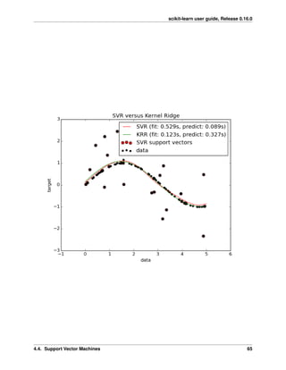

![scikit-learn user guide, Release 0.16.0
• If the number of features is much greater than the number of samples, the method is likely to give poor perfor-
mances.
• SVMs do not directly provide probability estimates, these are calculated using an expensive five-fold cross-
validation (see Scores and probabilities, below).
The support vector machines in scikit-learn support both dense (numpy.ndarray and convertible to that by
numpy.asarray) and sparse (any scipy.sparse) sample vectors as input. However, to use an SVM to make pre-
dictions for sparse data, it must have been fit on such data. For optimal performance, use C-ordered numpy.ndarray
(dense) or scipy.sparse.csr_matrix (sparse) with dtype=float64.
4.4.1 Classification
SVC, NuSVC and LinearSVC are classes capable of performing multi-class classification on a dataset.
SVC and NuSVC are similar methods, but accept slightly different sets of parameters and have different mathematical
formulations (see section Mathematical formulation). On the other hand, LinearSVC is another implementation of
Support Vector Classification for the case of a linear kernel. Note that LinearSVC does not accept keyword kernel,
as this is assumed to be linear. It also lacks some of the members of SVC and NuSVC, like support_.
As other classifiers, SVC, NuSVC and LinearSVC take as input two arrays: an array X of size [n_samples,
n_features] holding the training samples, and an array y of class labels (strings or integers), size [n_samples]:
4.4. Support Vector Machines 67](https://image.slidesharecdn.com/scikit-learn0-150409112902-conversion-gate01/85/Scikit-learn-0-16-0-user-guide-77-320.jpg)
![scikit-learn user guide, Release 0.16.0
>>> from sklearn import svm
>>> X = [[0, 0], [1, 1]]
>>> y = [0, 1]
>>> clf = svm.SVC()
>>> clf.fit(X, y)
SVC(C=1.0, cache_size=200, class_weight=None, coef0=0.0, degree=3,
gamma=0.0, kernel='rbf', max_iter=-1, probability=False, random_state=None,
shrinking=True, tol=0.001, verbose=False)
After being fitted, the model can then be used to predict new values:
>>> clf.predict([[2., 2.]])
array([1])
SVMs decision function depends on some subset of the training data, called the support vectors. Some properties of
these support vectors can be found in members support_vectors_, support_ and n_support:
>>> # get support vectors
>>> clf.support_vectors_
array([[ 0., 0.],
[ 1., 1.]])
>>> # get indices of support vectors
>>> clf.support_
array([0, 1]...)
>>> # get number of support vectors for each class
>>> clf.n_support_
array([1, 1]...)
Multi-class classification
SVC and NuSVC implement the “one-against-one” approach (Knerr et al., 1990) for multi- class classification. If
n_class is the number of classes, then n_class * (n_class - 1) / 2 classifiers are constructed and each
one trains data from two classes:
>>> X = [[0], [1], [2], [3]]
>>> Y = [0, 1, 2, 3]
>>> clf = svm.SVC()
>>> clf.fit(X, Y)
SVC(C=1.0, cache_size=200, class_weight=None, coef0=0.0, degree=3,
gamma=0.0, kernel='rbf', max_iter=-1, probability=False, random_state=None,
shrinking=True, tol=0.001, verbose=False)
>>> dec = clf.decision_function([[1]])
>>> dec.shape[1] # 4 classes: 4*3/2 = 6
6
On the other hand, LinearSVC implements “one-vs-the-rest” multi-class strategy, thus training n_class models. If
there are only two classes, only one model is trained:
>>> lin_clf = svm.LinearSVC()
>>> lin_clf.fit(X, Y)
LinearSVC(C=1.0, class_weight=None, dual=True, fit_intercept=True,
intercept_scaling=1, loss='squared_hinge', max_iter=1000,
multi_class='ovr', penalty='l2', random_state=None, tol=0.0001,
verbose=0)
>>> dec = lin_clf.decision_function([[1]])
>>> dec.shape[1]
4
68 Chapter 4. Supervised learning](https://image.slidesharecdn.com/scikit-learn0-150409112902-conversion-gate01/85/Scikit-learn-0-16-0-user-guide-78-320.jpg)
![scikit-learn user guide, Release 0.16.0
See Mathematical formulation for a complete description of the decision function.
Note that the LinearSVC also implements an alternative multi-class strategy, the so-called multi-class SVM formu-
lated by Crammer and Singer, by using the option multi_class=’crammer_singer’. This method is consis-
tent, which is not true for one-vs-rest classification. In practice, one-vs-rest classification is usually preferred, since
the results are mostly similar, but the runtime is significantly less.
For “one-vs-rest” LinearSVC the attributes coef_ and intercept_ have the shape [n_class,
n_features] and [n_class] respectively. Each row of the coefficients corresponds to one of the n_class
many “one-vs-rest” classifiers and similar for the intercepts, in the order of the “one” class.
In the case of “one-vs-one” SVC, the layout of the attributes is a little more involved. In the case of having a linear
kernel, The layout of coef_ and intercept_ is similar to the one described for LinearSVC described above,
except that the shape of coef_ is [n_class * (n_class - 1) / 2, n_features], corresponding to as
many binary classifiers. The order for classes 0 to n is “0 vs 1”, “0 vs 2” , ... “0 vs n”, “1 vs 2”, “1 vs 3”, “1 vs n”, . . .
“n-1 vs n”.
The shape of dual_coef_ is [n_class-1, n_SV] with a somewhat hard to grasp layout. The columns corre-
spond to the support vectors involved in any of the n_class * (n_class - 1) / 2 “one-vs-one” classifiers.
Each of the support vectors is used in n_class - 1 classifiers. The n_class - 1 entries in each row correspond
to the dual coefficients for these classifiers.
This might be made more clear by an example:
Consider a three class problem with with class 0 having three support vectors 𝑣0
0, 𝑣1
0, 𝑣2
0 and class 1 and 2 having two
support vectors 𝑣0
1, 𝑣1
1 and 𝑣0
2, 𝑣1
2 respectively. For each support vector 𝑣 𝑗
𝑖 , there are two dual coefficients. Let’s call
the coefficient of support vector 𝑣 𝑗
𝑖 in the classifier between classes 𝑖 and 𝑘 𝛼 𝑗
𝑖,𝑘. Then dual_coef_ looks like this:
𝛼0
0,1 𝛼0
0,2
Coefficients for SVs of class 0𝛼1
0,1 𝛼1
0,2
𝛼2
0,1 𝛼2
0,2
𝛼0
1,0 𝛼0
1,2
Coefficients for SVs of class 1
𝛼1
1,0 𝛼1
1,2
𝛼0
2,0 𝛼0
2,1
Coefficients for SVs of class 2
𝛼1
2,0 𝛼1
2,1
Scores and probabilities
The SVC method decision_function gives per-class scores for each sample (or a single score per sample in the
binary case). When the constructor option probability is set to True, class membership probability estimates
(from the methods predict_proba and predict_log_proba) are enabled. In the binary case, the probabilities
are calibrated using Platt scaling: logistic regression on the SVM’s scores, fit by an additional cross-validation on the
training data. In the multiclass case, this is extended as per Wu et al. (2004).
Needless to say, the cross-validation involved in Platt scaling is an expensive operation for large datasets. In addition,
the probability estimates may be inconsistent with the scores, in the sense that the “argmax” of the scores may not be
the argmax of the probabilities. (E.g., in binary classification, a sample may be labeled by predict as belonging
to a class that has probability <½ according to predict_proba.) Platt’s method is also known to have theoret-
ical issues. If confidence scores are required, but these do not have to be probabilities, then it is advisable to set
probability=False and use decision_function instead of predict_proba.
References:
• Wu, Lin and Weng, “Probability estimates for multi-class classification by pairwise coupling”. JMLR
5:975-1005, 2004.
4.4. Support Vector Machines 69](https://image.slidesharecdn.com/scikit-learn0-150409112902-conversion-gate01/85/Scikit-learn-0-16-0-user-guide-79-320.jpg)
![scikit-learn user guide, Release 0.16.0
Unbalanced problems
In problems where it is desired to give more importance to certain classes or certain individual samples keywords
class_weight and sample_weight can be used.
SVC (but not NuSVC) implement a keyword class_weight in the fit method. It’s a dictionary of the form
{class_label : value}, where value is a floating point number > 0 that sets the parameter C of class
class_label to C * value.
SVC, NuSVC, SVR, NuSVR and OneClassSVM implement also weights for individual samples in method fit
through keyword sample_weight. Similar to class_weight, these set the parameter C for the i-th example to
C * sample_weight[i].
70 Chapter 4. Supervised learning](https://image.slidesharecdn.com/scikit-learn0-150409112902-conversion-gate01/85/Scikit-learn-0-16-0-user-guide-80-320.jpg)
![scikit-learn user guide, Release 0.16.0
Examples:
• Plot different SVM classifiers in the iris dataset,
• SVM: Maximum margin separating hyperplane,
• SVM: Separating hyperplane for unbalanced classes
• SVM-Anova: SVM with univariate feature selection,
• Non-linear SVM
• SVM: Weighted samples,
4.4.2 Regression
The method of Support Vector Classification can be extended to solve regression problems. This method is called
Support Vector Regression.
The model produced by support vector classification (as described above) depends only on a subset of the training
data, because the cost function for building the model does not care about training points that lie beyond the margin.
Analogously, the model produced by Support Vector Regression depends only on a subset of the training data, because
the cost function for building the model ignores any training data close to the model prediction.
There are three different implementations of Support Vector Regression: SVR, NuSVR and LinearSVR.
LinearSVR provides a faster implementation than SVR but only considers linear kernels, while NuSVR implements
a slightly different formulation than SVR and LinearSVR. See Implementation details for further details.
As with classification classes, the fit method will take as argument vectors X, y, only that in this case y is expected to
have floating point values instead of integer values:
>>> from sklearn import svm
>>> X = [[0, 0], [2, 2]]
>>> y = [0.5, 2.5]
>>> clf = svm.SVR()
>>> clf.fit(X, y)
SVR(C=1.0, cache_size=200, coef0=0.0, degree=3, epsilon=0.1, gamma=0.0,
kernel='rbf', max_iter=-1, shrinking=True, tol=0.001, verbose=False)
>>> clf.predict([[1, 1]])
array([ 1.5])
Examples:
• Support Vector Regression (SVR) using linear and non-linear kernels
4.4.3 Density estimation, novelty detection
One-class SVM is used for novelty detection, that is, given a set of samples, it will detect the soft boundary of that set
so as to classify new points as belonging to that set or not. The class that implements this is called OneClassSVM.
In this case, as it is a type of unsupervised learning, the fit method will only take as input an array X, as there are no
class labels.
See, section Novelty and Outlier Detection for more details on this usage.
4.4. Support Vector Machines 71](https://image.slidesharecdn.com/scikit-learn0-150409112902-conversion-gate01/85/Scikit-learn-0-16-0-user-guide-81-320.jpg)
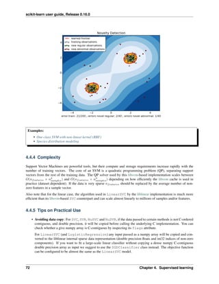
![scikit-learn user guide, Release 0.16.0
• Kernel cache size: For SVC, SVR, nuSVC and NuSVR, the size of the kernel cache has a strong impact on run
times for larger problems. If you have enough RAM available, it is recommended to set cache_size to a
higher value than the default of 200(MB), such as 500(MB) or 1000(MB).
• Setting C: C is 1 by default and it’s a reasonable default choice. If you have a lot of noisy observations you
should decrease it. It corresponds to regularize more the estimation.
• Support Vector Machine algorithms are not scale invariant, so it is highly recommended to scale your data.
For example, scale each attribute on the input vector X to [0,1] or [-1,+1], or standardize it to have mean 0
and variance 1. Note that the same scaling must be applied to the test vector to obtain meaningful results. See
section Preprocessing data for more details on scaling and normalization.
• Parameter nu in NuSVC/OneClassSVM/NuSVR approximates the fraction of training errors and support vec-
tors.
• In SVC, if data for classification are unbalanced (e.g. many positive and few negative), set
class_weight=’auto’ and/or try different penalty parameters C.
• The underlying LinearSVC implementation uses a random number generator to select features when fitting
the model. It is thus not uncommon, to have slightly different results for the same input data. If that happens,
try with a smaller tol parameter.
• Using L1 penalization as provided by LinearSVC(loss=’l2’, penalty=’l1’, dual=False)
yields a sparse solution, i.e. only a subset of feature weights is different from zero and contribute to the de-
cision function. Increasing C yields a more complex model (more feature are selected). The C value that yields
a “null” model (all weights equal to zero) can be calculated using l1_min_c.
4.4.6 Kernel functions
The kernel function can be any of the following:
• linear: ⟨𝑥, 𝑥′
⟩.
• polynomial: (𝛾⟨𝑥, 𝑥′
⟩ + 𝑟) 𝑑
. 𝑑 is specified by keyword degree, 𝑟 by coef0.
• rbf: exp(−𝛾|𝑥 − 𝑥′
|2
). 𝛾 is specified by keyword gamma, must be greater than 0.
• sigmoid (tanh(𝛾⟨𝑥, 𝑥′
⟩ + 𝑟)), where 𝑟 is specified by coef0.
Different kernels are specified by keyword kernel at initialization:
>>> linear_svc = svm.SVC(kernel='linear')
>>> linear_svc.kernel
'linear'
>>> rbf_svc = svm.SVC(kernel='rbf')
>>> rbf_svc.kernel
'rbf'
Custom Kernels
You can define your own kernels by either giving the kernel as a python function or by precomputing the Gram matrix.
Classifiers with custom kernels behave the same way as any other classifiers, except that:
• Field support_vectors_ is now empty, only indices of support vectors are stored in support_
• A reference (and not a copy) of the first argument in the fit() method is stored for future reference. If that
array changes between the use of fit() and predict() you will have unexpected results.
4.4. Support Vector Machines 73](https://image.slidesharecdn.com/scikit-learn0-150409112902-conversion-gate01/85/Scikit-learn-0-16-0-user-guide-83-320.jpg)
![scikit-learn user guide, Release 0.16.0
Using Python functions as kernels
You can also use your own defined kernels by passing a function to the keyword kernel in the constructor.
Your kernel must take as arguments two matrices and return a third matrix.
The following code defines a linear kernel and creates a classifier instance that will use that kernel:
>>> import numpy as np
>>> from sklearn import svm
>>> def my_kernel(x, y):
... return np.dot(x, y.T)
...
>>> clf = svm.SVC(kernel=my_kernel)
Examples:
• SVM with custom kernel.
Using the Gram matrix
Set kernel=’precomputed’ and pass the Gram matrix instead of X in the fit method. At the moment, the kernel
values between all training vectors and the test vectors must be provided.
>>> import numpy as np
>>> from sklearn import svm
>>> X = np.array([[0, 0], [1, 1]])
>>> y = [0, 1]
>>> clf = svm.SVC(kernel='precomputed')
>>> # linear kernel computation
>>> gram = np.dot(X, X.T)
>>> clf.fit(gram, y)
SVC(C=1.0, cache_size=200, class_weight=None, coef0=0.0, degree=3,
gamma=0.0, kernel='precomputed', max_iter=-1, probability=False,
random_state=None, shrinking=True, tol=0.001, verbose=False)
>>> # predict on training examples
>>> clf.predict(gram)
array([0, 1])
Parameters of the RBF Kernel
When training an SVM with the Radial Basis Function (RBF) kernel, two parameters must be considered: C and
gamma. The parameter C, common to all SVM kernels, trades off misclassification of training examples against
simplicity of the decision surface. A low C makes the decision surface smooth, while a high C aims at classifying all
training examples correctly. gamma defines how much influence a single training example has. The larger gamma is,
the closer other examples must be to be affected.
Proper choice of C and gamma is critical to the SVM’s performance. One is advised to use
sklearn.grid_search.GridSearchCV with C and gamma spaced exponentially far apart to choose good
values.
74 Chapter 4. Supervised learning](https://image.slidesharecdn.com/scikit-learn0-150409112902-conversion-gate01/85/Scikit-learn-0-16-0-user-guide-84-320.jpg)

![scikit-learn user guide, Release 0.16.0
where 𝑒 is the vector of all ones, 𝐶 > 0 is the upper bound, 𝑄 is an 𝑛 by 𝑛 positive semidefinite matrix, 𝑄𝑖𝑗 ≡
𝐾(𝑥𝑖, 𝑥 𝑗) = 𝜑(𝑥𝑖) 𝑇
𝜑(𝑥 𝑗) is the kernel. Here training vectors are implicitly mapped into a higher (maybe infinite)
dimensional space by the function 𝜑.
The decision function is:
sgn(
𝑛∑︁
𝑖=1
𝑦𝑖 𝛼𝑖 𝐾(𝑥𝑖, 𝑥) + 𝜌)
Note: While SVM models derived from libsvm and liblinear use C as regularization parameter, most other estimators
use alpha. The relation between both is 𝐶 = 𝑛_𝑠𝑎𝑚𝑝𝑙𝑒𝑠
𝑎𝑙𝑝ℎ𝑎 .
This parameters can be accessed through the members dual_coef_ which holds the product 𝑦𝑖 𝛼𝑖,
support_vectors_ which holds the support vectors, and intercept_ which holds the independent term 𝜌
:
References:
• “Automatic Capacity Tuning of Very Large VC-dimension Classifiers” I Guyon, B Boser, V Vapnik -
Advances in neural information processing 1993,
• “Support-vector networks” C. Cortes, V. Vapnik, Machine Leaming, 20, 273-297 (1995)
NuSVC
We introduce a new parameter 𝜈 which controls the number of support vectors and training errors. The parameter
𝜈 ∈ (0, 1] is an upper bound on the fraction of training errors and a lower bound of the fraction of support vectors.
It can be shown that the 𝜈-SVC formulation is a reparametrization of the 𝐶-SVC and therefore mathematically equiv-
alent.
SVR
Given training vectors 𝑥𝑖 ∈ R 𝑝
, i=1,..., n, and a vector 𝑦 ∈ R 𝑛
𝜀-SVR solves the following primal problem:
min
𝑤,𝑏,𝜁,𝜁*
1
2
𝑤 𝑇
𝑤 + 𝐶
𝑛∑︁
𝑖=1
(𝜁𝑖 + 𝜁*
𝑖 )
subject to 𝑦𝑖 − 𝑤 𝑇
𝜑(𝑥𝑖) − 𝑏 ≤ 𝜀 + 𝜁𝑖,
𝑤 𝑇
𝜑(𝑥𝑖) + 𝑏 − 𝑦𝑖 ≤ 𝜀 + 𝜁*
𝑖 ,
𝜁𝑖, 𝜁*
𝑖 ≥ 0, 𝑖 = 1, ..., 𝑛
Its dual is
min
𝛼,𝛼*
1
2
(𝛼 − 𝛼*
) 𝑇
𝑄(𝛼 − 𝛼*
) + 𝜀𝑒 𝑇
(𝛼 + 𝛼*
) − 𝑦 𝑇
(𝛼 − 𝛼*
)
subject to 𝑒 𝑇
(𝛼 − 𝛼*
) = 0
0 ≤ 𝛼𝑖, 𝛼*
𝑖 ≤ 𝐶, 𝑖 = 1, ..., 𝑛
where 𝑒 is the vector of all ones, 𝐶 > 0 is the upper bound, 𝑄 is an 𝑛 by 𝑛 positive semidefinite matrix, 𝑄𝑖𝑗 ≡
𝐾(𝑥𝑖, 𝑥 𝑗) = 𝜑(𝑥𝑖) 𝑇
𝜑(𝑥 𝑗) is the kernel. Here training vectors are implicitly mapped into a higher (maybe infinite)
dimensional space by the function 𝜑.
76 Chapter 4. Supervised learning](https://image.slidesharecdn.com/scikit-learn0-150409112902-conversion-gate01/85/Scikit-learn-0-16-0-user-guide-86-320.jpg)
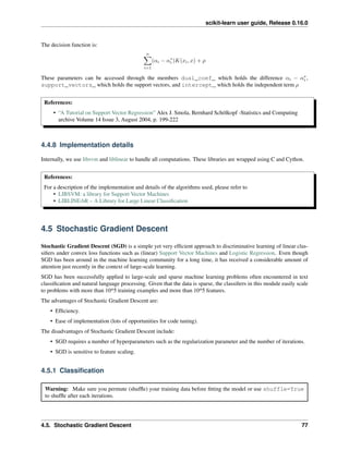
![scikit-learn user guide, Release 0.16.0
The class SGDClassifier implements a plain stochastic gradient descent learning routine which supports different
loss functions and penalties for classification.
As other classifiers, SGD has to be fitted with two arrays: an array X of size [n_samples, n_features] holding the
training samples, and an array Y of size [n_samples] holding the target values (class labels) for the training samples:
>>> from sklearn.linear_model import SGDClassifier
>>> X = [[0., 0.], [1., 1.]]
>>> y = [0, 1]
>>> clf = SGDClassifier(loss="hinge", penalty="l2")
>>> clf.fit(X, y)
SGDClassifier(alpha=0.0001, average=False, class_weight=None, epsilon=0.1,
eta0=0.0, fit_intercept=True, l1_ratio=0.15,
learning_rate='optimal', loss='hinge', n_iter=5, n_jobs=1,
penalty='l2', power_t=0.5, random_state=None, shuffle=True,
verbose=0, warm_start=False)
After being fitted, the model can then be used to predict new values:
>>> clf.predict([[2., 2.]])
array([1])
SGD fits a linear model to the training data. The member coef_ holds the model parameters:
>>> clf.coef_
array([[ 9.9..., 9.9...]])
Member intercept_ holds the intercept (aka offset or bias):
>>> clf.intercept_
array([-9.9...])
Whether or not the model should use an intercept, i.e. a biased hyperplane, is controlled by the parameter
fit_intercept.
78 Chapter 4. Supervised learning](https://image.slidesharecdn.com/scikit-learn0-150409112902-conversion-gate01/85/Scikit-learn-0-16-0-user-guide-88-320.jpg)
![scikit-learn user guide, Release 0.16.0
To get the signed distance to the hyperplane use SGDClassifier.decision_function:
>>> clf.decision_function([[2., 2.]])
array([ 29.6...])
The concrete loss function can be set via the loss parameter. SGDClassifier supports the following loss func-
tions:
• loss="hinge": (soft-margin) linear Support Vector Machine,
• loss="modified_huber": smoothed hinge loss,
• loss="log": logistic regression,
• and all regression losses below.
The first two loss functions are lazy, they only update the model parameters if an example violates the margin con-
straint, which makes training very efficient and may result in sparser models, even when L2 penalty is used.
Using loss="log" or loss="modified_huber" enables the predict_proba method, which gives a vector
of probability estimates 𝑃(𝑦|𝑥) per sample 𝑥:
>>> clf = SGDClassifier(loss="log").fit(X, y)
>>> clf.predict_proba([[1., 1.]])
array([[ 0.00..., 0.99...]])
The concrete penalty can be set via the penalty parameter. SGD supports the following penalties:
• penalty="l2": L2 norm penalty on coef_.
• penalty="l1": L1 norm penalty on coef_.
• penalty="elasticnet": Convex combination of L2 and L1; (1 - l1_ratio) * L2 +
l1_ratio * L1.
The default setting is penalty="l2". The L1 penalty leads to sparse solutions, driving most coefficients to zero.
The Elastic Net solves some deficiencies of the L1 penalty in the presence of highly correlated attributes. The param-
eter l1_ratio controls the convex combination of L1 and L2 penalty.
SGDClassifier supports multi-class classification by combining multiple binary classifiers in a “one versus all”
(OVA) scheme. For each of the 𝐾 classes, a binary classifier is learned that discriminates between that and all other
𝐾 − 1 classes. At testing time, we compute the confidence score (i.e. the signed distances to the hyperplane) for each
classifier and choose the class with the highest confidence. The Figure below illustrates the OVA approach on the iris
dataset. The dashed lines represent the three OVA classifiers; the background colors show the decision surface induced
by the three classifiers.
In the case of multi-class classification coef_ is a two-dimensionally array of shape=[n_classes,
n_features] and intercept_ is a one dimensional array of shape=[n_classes]. The i-th row of coef_
holds the weight vector of the OVA classifier for the i-th class; classes are indexed in ascending order (see at-
tribute classes_). Note that, in principle, since they allow to create a probability model, loss="log" and
loss="modified_huber" are more suitable for one-vs-all classification.
SGDClassifier supports both weighted classes and weighted instances via the fit parameters class_weight and
sample_weight. See the examples below and the doc string of SGDClassifier.fit for further information.
Examples:
• SGD: Maximum margin separating hyperplane,
• Plot multi-class SGD on the iris dataset
• SGD: Weighted samples
• SVM: Separating hyperplane for unbalanced classes (See the Note)
4.5. Stochastic Gradient Descent 79](https://image.slidesharecdn.com/scikit-learn0-150409112902-conversion-gate01/85/Scikit-learn-0-16-0-user-guide-89-320.jpg)

![scikit-learn user guide, Release 0.16.0
There is built-in support for sparse data given in any matrix in a format supported by scipy.sparse. For maximum
efficiency, however, use the CSR matrix format as defined in scipy.sparse.csr_matrix.
Examples:
• Classification of text documents using sparse features
4.5.4 Complexity
The major advantage of SGD is its efficiency, which is basically linear in the number of training examples. If X is a
matrix of size (n, p) training has a cost of 𝑂(𝑘𝑛¯𝑝), where k is the number of iterations (epochs) and ¯𝑝 is the average
number of non-zero attributes per sample.
Recent theoretical results, however, show that the runtime to get some desired optimization accuracy does not increase
as the training set size increases.
4.5.5 Tips on Practical Use
• Stochastic Gradient Descent is sensitive to feature scaling, so it is highly recommended to scale your data. For
example, scale each attribute on the input vector X to [0,1] or [-1,+1], or standardize it to have mean 0 and
variance 1. Note that the same scaling must be applied to the test vector to obtain meaningful results. This can
be easily done using StandardScaler:
from sklearn.preprocessing import StandardScaler
scaler = StandardScaler()
scaler.fit(X_train) # Don't cheat - fit only on training data
X_train = scaler.transform(X_train)
X_test = scaler.transform(X_test) # apply same transformation to test data
If your attributes have an intrinsic scale (e.g. word frequencies or indicator features) scaling is not needed.
• Finding a reasonable regularization term 𝛼 is best done using GridSearchCV, usually in the range
10.0**-np.arange(1,7).
• Empirically, we found that SGD converges after observing approx. 10^6 training samples. Thus, a reasonable
first guess for the number of iterations is n_iter = np.ceil(10**6 / n), where n is the size of the
training set.
• If you apply SGD to features extracted using PCA we found that it is often wise to scale the feature values by
some constant c such that the average L2 norm of the training data equals one.
• We found that Averaged SGD works best with a larger number of features and a higher eta0
References:
• “Efficient BackProp” Y. LeCun, L. Bottou, G. Orr, K. Müller - In Neural Networks: Tricks of the Trade
1998.
4.5.6 Mathematical formulation
Given a set of training examples (𝑥1, 𝑦1), . . . , (𝑥 𝑛, 𝑦 𝑛) where 𝑥𝑖 ∈ R 𝑛
and 𝑦𝑖 ∈ {−1, 1}, our goal is to learn a linear
scoring function 𝑓(𝑥) = 𝑤 𝑇
𝑥 + 𝑏 with model parameters 𝑤 ∈ R 𝑚
and intercept 𝑏 ∈ R. In order to make predictions,
4.5. Stochastic Gradient Descent 81](https://image.slidesharecdn.com/scikit-learn0-150409112902-conversion-gate01/85/Scikit-learn-0-16-0-user-guide-91-320.jpg)
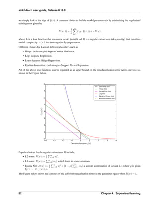

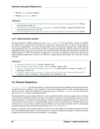
![scikit-learn user guide, Release 0.16.0
The classes in sklearn.neighbors can handle either Numpy arrays or scipy.sparse matrices as input. For dense
matrices, a large number of possible distance metrics are supported. For sparse matrices, arbitrary Minkowski metrics
are supported for searches.
There are many learning routines which rely on nearest neighbors at their core. One example is kernel density estima-
tion, discussed in the density estimation section.
4.6.1 Unsupervised Nearest Neighbors
NearestNeighbors implements unsupervised nearest neighbors learning. It acts as a uniform interface to three
different nearest neighbors algorithms: BallTree, KDTree, and a brute-force algorithm based on routines in
sklearn.metrics.pairwise. The choice of neighbors search algorithm is controlled through the keyword
’algorithm’, which must be one of [’auto’, ’ball_tree’, ’kd_tree’, ’brute’]. When the de-
fault value ’auto’ is passed, the algorithm attempts to determine the best approach from the training data. For a
discussion of the strengths and weaknesses of each option, see Nearest Neighbor Algorithms.
Warning: Regarding the Nearest Neighbors algorithms, if two neighbors, neighbor 𝑘 +1 and 𝑘, have
identical distances but different labels, the results will depend on the ordering of the training data.
Finding the Nearest Neighbors
For the simple task of finding the nearest neighbors between two sets of data, the unsupervised algorithms within
sklearn.neighbors can be used:
>>> from sklearn.neighbors import NearestNeighbors
>>> import numpy as np
>>> X = np.array([[-1, -1], [-2, -1], [-3, -2], [1, 1], [2, 1], [3, 2]])
>>> nbrs = NearestNeighbors(n_neighbors=2, algorithm='ball_tree').fit(X)
>>> distances, indices = nbrs.kneighbors(X)
>>> indices
array([[0, 1],
[1, 0],
[2, 1],
[3, 4],
[4, 3],
[5, 4]]...)
>>> distances
array([[ 0. , 1. ],
[ 0. , 1. ],
[ 0. , 1.41421356],
[ 0. , 1. ],
[ 0. , 1. ],
[ 0. , 1.41421356]])
Because the query set matches the training set, the nearest neighbor of each point is the point itself, at a distance of
zero.
It is also possible to efficiently produce a sparse graph showing the connections between neighboring points:
>>> nbrs.kneighbors_graph(X).toarray()
array([[ 1., 1., 0., 0., 0., 0.],
[ 1., 1., 0., 0., 0., 0.],
[ 0., 1., 1., 0., 0., 0.],
[ 0., 0., 0., 1., 1., 0.],
[ 0., 0., 0., 1., 1., 0.],
[ 0., 0., 0., 0., 1., 1.]])
4.6. Nearest Neighbors 85](https://image.slidesharecdn.com/scikit-learn0-150409112902-conversion-gate01/85/Scikit-learn-0-16-0-user-guide-95-320.jpg)
![scikit-learn user guide, Release 0.16.0
Our dataset is structured such that points nearby in index order are nearby in parameter space, leading to
an approximately block-diagonal matrix of K-nearest neighbors. Such a sparse graph is useful in a vari-
ety of circumstances which make use of spatial relationships between points for unsupervised learning: in
particular, see sklearn.manifold.Isomap, sklearn.manifold.LocallyLinearEmbedding, and
sklearn.cluster.SpectralClustering.
KDTree and BallTree Classes
Alternatively, one can use the KDTree or BallTree classes directly to find nearest neighbors. This is the function-
ality wrapped by the NearestNeighbors class used above. The Ball Tree and KD Tree have the same interface;
we’ll show an example of using the KD Tree here:
>>> from sklearn.neighbors import KDTree
>>> import numpy as np
>>> X = np.array([[-1, -1], [-2, -1], [-3, -2], [1, 1], [2, 1], [3, 2]])
>>> kdt = KDTree(X, leaf_size=30, metric='euclidean')
>>> kdt.query(X, k=2, return_distance=False)
array([[0, 1],
[1, 0],
[2, 1],
[3, 4],
[4, 3],
[5, 4]]...)
Refer to the KDTree and BallTree class documentation for more information on the options available for neighbors
searches, including specification of query strategies, of various distance metrics, etc. For a list of available metrics,
see the documentation of the DistanceMetric class.
4.6.2 Nearest Neighbors Classification
Neighbors-based classification is a type of instance-based learning or non-generalizing learning: it does not attempt
to construct a general internal model, but simply stores instances of the training data. Classification is computed from
a simple majority vote of the nearest neighbors of each point: a query point is assigned the data class which has the
most representatives within the nearest neighbors of the point.
scikit-learn implements two different nearest neighbors classifiers: KNeighborsClassifier implements learn-
ing based on the 𝑘 nearest neighbors of each query point, where 𝑘 is an integer value specified by the user.
RadiusNeighborsClassifier implements learning based on the number of neighbors within a fixed radius
𝑟 of each training point, where 𝑟 is a floating-point value specified by the user.
The 𝑘-neighbors classification in KNeighborsClassifier is the more commonly used of the two techniques.
The optimal choice of the value 𝑘 is highly data-dependent: in general a larger 𝑘 suppresses the effects of noise, but
makes the classification boundaries less distinct.
In cases where the data is not uniformly sampled, radius-based neighbors classification in
RadiusNeighborsClassifier can be a better choice. The user specifies a fixed radius 𝑟, such that
points in sparser neighborhoods use fewer nearest neighbors for the classification. For high-dimensional parameter
spaces, this method becomes less effective due to the so-called “curse of dimensionality”.
The basic nearest neighbors classification uses uniform weights: that is, the value assigned to a query point is computed
from a simple majority vote of the nearest neighbors. Under some circumstances, it is better to weight the neighbors
such that nearer neighbors contribute more to the fit. This can be accomplished through the weights keyword. The
default value, weights = ’uniform’, assigns uniform weights to each neighbor. weights = ’distance’
assigns weights proportional to the inverse of the distance from the query point. Alternatively, a user-defined function
of the distance can be supplied which is used to compute the weights.
86 Chapter 4. Supervised learning](https://image.slidesharecdn.com/scikit-learn0-150409112902-conversion-gate01/85/Scikit-learn-0-16-0-user-guide-96-320.jpg)

![scikit-learn user guide, Release 0.16.0
the lower half of those faces.
Examples:
• Nearest Neighbors regression: an example of regression using nearest neighbors.
• Face completion with a multi-output estimators: an example of multi-output regression using nearest
neighbors.
4.6.4 Nearest Neighbor Algorithms
Brute Force
Fast computation of nearest neighbors is an active area of research in machine learning. The most naive neighbor
search implementation involves the brute-force computation of distances between all pairs of points in the dataset:
for 𝑁 samples in 𝐷 dimensions, this approach scales as 𝑂[𝐷𝑁2
]. Efficient brute-force neighbors searches can
be very competitive for small data samples. However, as the number of samples 𝑁 grows, the brute-force ap-
proach quickly becomes infeasible. In the classes within sklearn.neighbors, brute-force neighbors searches
are specified using the keyword algorithm = ’brute’, and are computed using the routines available in
sklearn.metrics.pairwise.
K-D Tree
To address the computational inefficiencies of the brute-force approach, a variety of tree-based data structures have
been invented. In general, these structures attempt to reduce the required number of distance calculations by efficiently
encoding aggregate distance information for the sample. The basic idea is that if point 𝐴 is very distant from point
𝐵, and point 𝐵 is very close to point 𝐶, then we know that points 𝐴 and 𝐶 are very distant, without having to
explicitly calculate their distance. In this way, the computational cost of a nearest neighbors search can be reduced to
𝑂[𝐷𝑁 log(𝑁)] or better. This is a significant improvement over brute-force for large 𝑁.
88 Chapter 4. Supervised learning](https://image.slidesharecdn.com/scikit-learn0-150409112902-conversion-gate01/85/Scikit-learn-0-16-0-user-guide-98-320.jpg)

![scikit-learn user guide, Release 0.16.0
An early approach to taking advantage of this aggregate information was the KD tree data structure (short for K-
dimensional tree), which generalizes two-dimensional Quad-trees and 3-dimensional Oct-trees to an arbitrary number
of dimensions. The KD tree is a binary tree structure which recursively partitions the parameter space along the data
axes, dividing it into nested orthotopic regions into which data points are filed. The construction of a KD tree is very
fast: because partitioning is performed only along the data axes, no 𝐷-dimensional distances need to be computed.
Once constructed, the nearest neighbor of a query point can be determined with only 𝑂[log(𝑁)] distance computations.
Though the KD tree approach is very fast for low-dimensional (𝐷 < 20) neighbors searches, it becomes inefficient
as 𝐷 grows very large: this is one manifestation of the so-called “curse of dimensionality”. In scikit-learn, KD tree
neighbors searches are specified using the keyword algorithm = ’kd_tree’, and are computed using the class
KDTree.
References:
• “Multidimensional binary search trees used for associative searching”, Bentley, J.L., Communications of
the ACM (1975)
Ball Tree
To address the inefficiencies of KD Trees in higher dimensions, the ball tree data structure was developed. Where
KD trees partition data along Cartesian axes, ball trees partition data in a series of nesting hyper-spheres. This makes
tree construction more costly than that of the KD tree, but results in a data structure which can be very efficient on
highly-structured data, even in very high dimensions.
A ball tree recursively divides the data into nodes defined by a centroid 𝐶 and radius 𝑟, such that each point in the
node lies within the hyper-sphere defined by 𝑟 and 𝐶. The number of candidate points for a neighbor search is reduced
through use of the triangle inequality:
|𝑥 + 𝑦| ≤ |𝑥| + |𝑦|
With this setup, a single distance calculation between a test point and the centroid is sufficient to determine a lower
and upper bound on the distance to all points within the node. Because of the spherical geometry of the ball tree nodes,
it can out-perform a KD-tree in high dimensions, though the actual performance is highly dependent on the structure
of the training data. In scikit-learn, ball-tree-based neighbors searches are specified using the keyword algorithm
= ’ball_tree’, and are computed using the class sklearn.neighbors.BallTree. Alternatively, the user
can work with the BallTree class directly.
References:
• “Five balltree construction algorithms”, Omohundro, S.M., International Computer Science Institute Tech-
nical Report (1989)
Choice of Nearest Neighbors Algorithm
The optimal algorithm for a given dataset is a complicated choice, and depends on a number of factors:
• number of samples 𝑁 (i.e. n_samples) and dimensionality 𝐷 (i.e. n_features).
– Brute force query time grows as 𝑂[𝐷𝑁]
– Ball tree query time grows as approximately 𝑂[𝐷 log(𝑁)]
– KD tree query time changes with 𝐷 in a way that is difficult to precisely characterise. For small 𝐷 (less
than 20 or so) the cost is approximately 𝑂[𝐷 log(𝑁)], and the KD tree query can be very efficient. For
90 Chapter 4. Supervised learning](https://image.slidesharecdn.com/scikit-learn0-150409112902-conversion-gate01/85/Scikit-learn-0-16-0-user-guide-100-320.jpg)
![scikit-learn user guide, Release 0.16.0
larger 𝐷, the cost increases to nearly 𝑂[𝐷𝑁], and the overhead due to the tree structure can lead to queries
which are slower than brute force.
For small data sets (𝑁 less than 30 or so), log(𝑁) is comparable to 𝑁, and brute force algorithms can be more
efficient than a tree-based approach. Both KDTree and BallTree address this through providing a leaf size
parameter: this controls the number of samples at which a query switches to brute-force. This allows both
algorithms to approach the efficiency of a brute-force computation for small 𝑁.
• data structure: intrinsic dimensionality of the data and/or sparsity of the data. Intrinsic dimensionality refers
to the dimension 𝑑 ≤ 𝐷 of a manifold on which the data lies, which can be linearly or non-linearly embedded
in the parameter space. Sparsity refers to the degree to which the data fills the parameter space (this is to be
distinguished from the concept as used in “sparse” matrices. The data matrix may have no zero entries, but the
structure can still be “sparse” in this sense).
– Brute force query time is unchanged by data structure.
– Ball tree and KD tree query times can be greatly influenced by data structure. In general, sparser data with a
smaller intrinsic dimensionality leads to faster query times. Because the KD tree internal representation is
aligned with the parameter axes, it will not generally show as much improvement as ball tree for arbitrarily
structured data.
Datasets used in machine learning tend to be very structured, and are very well-suited for tree-based queries.
• number of neighbors 𝑘 requested for a query point.
– Brute force query time is largely unaffected by the value of 𝑘
– Ball tree and KD tree query time will become slower as 𝑘 increases. This is due to two effects: first, a
larger 𝑘 leads to the necessity to search a larger portion of the parameter space. Second, using 𝑘 > 1
requires internal queueing of results as the tree is traversed.
As 𝑘 becomes large compared to 𝑁, the ability to prune branches in a tree-based query is reduced. In this
situation, Brute force queries can be more efficient.
• number of query points. Both the ball tree and the KD Tree require a construction phase. The cost of this
construction becomes negligible when amortized over many queries. If only a small number of queries will
be performed, however, the construction can make up a significant fraction of the total cost. If very few query
points will be required, brute force is better than a tree-based method.
Currently, algorithm = ’auto’ selects ’kd_tree’ if 𝑘 < 𝑁/2 and the ’effective_metric_’
is in the ’VALID_METRICS’ list of ’kd_tree’. It selects ’ball_tree’ if 𝑘 < 𝑁/2 and the
’effective_metric_’ is not in the ’VALID_METRICS’ list of ’kd_tree’. It selects ’brute’ if 𝑘 >=
𝑁/2. This choice is based on the assumption that the number of query points is at least the same order as the number
of training points, and that leaf_size is close to its default value of 30.
Effect of leaf_size
As noted above, for small sample sizes a brute force search can be more efficient than a tree-based query. This fact is
accounted for in the ball tree and KD tree by internally switching to brute force searches within leaf nodes. The level
of this switch can be specified with the parameter leaf_size. This parameter choice has many effects:
construction time A larger leaf_size leads to a faster tree construction time, because fewer nodes need to be
created
query time Both a large or small leaf_size can lead to suboptimal query cost. For leaf_size approaching
1, the overhead involved in traversing nodes can significantly slow query times. For leaf_size approach-
ing the size of the training set, queries become essentially brute force. A good compromise between these is
leaf_size = 30, the default value of the parameter.
4.6. Nearest Neighbors 91](https://image.slidesharecdn.com/scikit-learn0-150409112902-conversion-gate01/85/Scikit-learn-0-16-0-user-guide-101-320.jpg)
![scikit-learn user guide, Release 0.16.0
memory As leaf_size increases, the memory required to store a tree structure decreases. This is especially
important in the case of ball tree, which stores a 𝐷-dimensional centroid for each node. The required storage
space for BallTree is approximately 1 / leaf_size times the size of the training set.
leaf_size is not referenced for brute force queries.
4.6.5 Nearest Centroid Classifier
The NearestCentroid classifier is a simple algorithm that represents each class by the centroid of its members. In
effect, this makes it similar to the label updating phase of the sklearn.KMeans algorithm. It also has no parameters
to choose, making it a good baseline classifier. It does, however, suffer on non-convex classes, as well as when classes
have drastically different variances, as equal variance in all dimensions is assumed. See Linear Discriminant Analysis
(sklearn.lda.LDA) and Quadratic Discriminant Analysis (sklearn.qda.QDA) for more complex methods that
do not make this assumption. Usage of the default NearestCentroid is simple:
>>> from sklearn.neighbors.nearest_centroid import NearestCentroid
>>> import numpy as np
>>> X = np.array([[-1, -1], [-2, -1], [-3, -2], [1, 1], [2, 1], [3, 2]])
>>> y = np.array([1, 1, 1, 2, 2, 2])
>>> clf = NearestCentroid()
>>> clf.fit(X, y)
NearestCentroid(metric='euclidean', shrink_threshold=None)
>>> print(clf.predict([[-0.8, -1]]))
[1]
Nearest Shrunken Centroid
The NearestCentroid classifier has a shrink_threshold parameter, which implements the nearest shrunken
centroid classifier. In effect, the value of each feature for each centroid is divided by the within-class variance of that
feature. The feature values are then reduced by shrink_threshold. Most notably, if a particular feature value
crosses zero, it is set to zero. In effect, this removes the feature from affecting the classification. This is useful, for
example, for removing noisy features.
In the example below, using a small shrink threshold increases the accuracy of the model from 0.81 to 0.82.
92 Chapter 4. Supervised learning](https://image.slidesharecdn.com/scikit-learn0-150409112902-conversion-gate01/85/Scikit-learn-0-16-0-user-guide-102-320.jpg)


![scikit-learn user guide, Release 0.16.0
A family 𝐻 of functions from a domain 𝑆 to a range 𝑈 is called (𝑟, 𝑒, 𝑝1, 𝑝2)-sensitive, with 𝑟, 𝑒 > 0, 𝑝1 > 𝑝2 > 0, if
for any 𝑝, 𝑞 ∈ 𝑆, the following conditions hold (𝐷 is the distance function):
• If 𝐷(𝑝, 𝑞) <= 𝑟 then 𝑃 𝐻[ℎ(𝑝) = ℎ(𝑞)] >= 𝑝1,
• If 𝐷(𝑝, 𝑞) > 𝑟(1 + 𝑒) then 𝑃 𝐻[ℎ(𝑝) = ℎ(𝑞)] <= 𝑝2.
As defined, nearby points within a distance of 𝑟 to each other are likely to collide with probability 𝑝1. In contrast,
distant points which are located with the distance more than 𝑟(1 + 𝑒) have a small probability of 𝑝2 of collision.
Suppose there is a family of LSH function 𝐻. An LSH index is built as follows:
1. Choose 𝑘 functions ℎ1, ℎ2, ...ℎ 𝑘 uniformly at random (with replacement) from 𝐻. For any 𝑝 ∈ 𝑆, place 𝑝 in
the bucket with label 𝑔(𝑝) = (ℎ1(𝑝), ℎ2(𝑝), ...ℎ 𝑘(𝑝)). Observe that if each ℎ𝑖 outputs one “digit”, each bucket
has a k-digit label.
2. Independently perform step 1 𝑙 times to construct 𝑙 separate estimators, with hash functions 𝑔1, 𝑔2, ... 𝑔𝑙.
The reason to concatenate hash functions in the step 1 is to decrease the probability of the collision of distant points
as much as possible. The probability drops from 𝑝2 to 𝑝 𝑘
2 which is negligibly small for large 𝑘. The choice of 𝑘 is
strongly dependent on the data set size and structure and is therefore hard to tune in practice. There is a side effect of
having a large 𝑘; it has the potential of decreasing the chance of nearby points getting collided. To address this issue,
multiple estimators are constructed in step 2.
The requirement to tune 𝑘 for a given dataset makes classical LSH cumbersome to use in practice. The LSH Forest
variant has benn designed to alleviate this requirement by automatically adjusting the number of digits used to hash
the samples.
LSH Forest is formulated with prefix trees with each leaf of a tree corresponding to an actual data point in the database.
There are 𝑙 such trees which compose the forest and they are constructed using independently drawn random sequence
of hash functions from 𝐻. In this implementation, “Random Projections” is being used as the LSH technique which is
an approximation for the cosine distance. The length of the sequence of hash functions is kept fixed at 32. Moreover,
a prefix tree is implemented using sorted arrays and binary search.
There are two phases of tree traversals used in order to answer a query to find the 𝑚 nearest neighbors of a point
𝑞. First, a top-down traversal is performed using a binary search to identify the leaf having the longest prefix match
(maximum depth) with 𝑞‘s label after subjecting 𝑞 to the same hash functions. 𝑀 >> 𝑚 points (total candidates)
are extracted from the forest, moving up from the previously found maximum depth towards the root synchronously
across all trees in the bottom-up traversal. M is set to 𝑐𝑙 where 𝑐, the number of candidates extracted from each tree,
is a constant. Finally, the similarity of each of these 𝑀 points against point 𝑞 is calculated and the top 𝑚 points are
returned as the nearest neighbors of 𝑞. Since most of the time in these queries is spent calculating the distances to
candidates, the speedup compared to brute force search is approximately 𝑁/𝑀, where 𝑁 is the number of points in
database.
96 Chapter 4. Supervised learning](https://image.slidesharecdn.com/scikit-learn0-150409112902-conversion-gate01/85/Scikit-learn-0-16-0-user-guide-106-320.jpg)
![scikit-learn user guide, Release 0.16.0
References:
• “Near-Optimal Hashing Algorithms for Approximate Nearest Neighbor in High Dimensions”, Alexandr,
A., Indyk, P., Foundations of Computer Science, 2006. FOCS ‘06. 47th Annual IEEE Symposium
• “LSH Forest: Self-Tuning Indexes for Similarity Search”, Bawa, M., Condie, T., Ganesan, P., WWW ‘05
Proceedings of the 14th international conference on World Wide Web Pages 651-660
4.7 Gaussian Processes
Gaussian Processes for Machine Learning (GPML) is a generic supervised learning method primarily designed to
solve regression problems. It has also been extended to probabilistic classification, but in the present implementation,
this is only a post-processing of the regression exercise.
The advantages of Gaussian Processes for Machine Learning are:
• The prediction interpolates the observations (at least for regular correlation models).
• The prediction is probabilistic (Gaussian) so that one can compute empirical confidence intervals and ex-
ceedance probabilities that might be used to refit (online fitting, adaptive fitting) the prediction in some region
of interest.
• Versatile: different linear regression models and correlation models can be specified. Common models are
provided, but it is also possible to specify custom models provided they are stationary.
The disadvantages of Gaussian Processes for Machine Learning include:
• It is not sparse. It uses the whole samples/features information to perform the prediction.
• It loses efficiency in high dimensional spaces – namely when the number of features exceeds a few dozens. It
might indeed give poor performance and it loses computational efficiency.
• Classification is only a post-processing, meaning that one first need to solve a regression problem by providing
the complete scalar float precision output 𝑦 of the experiment one attempt to model.
Thanks to the Gaussian property of the prediction, it has been given varied applications: e.g. for global optimization,
probabilistic classification.
4.7.1 Examples
An introductory regression example
Say we want to surrogate the function 𝑔(𝑥) = 𝑥 sin(𝑥). To do so, the function is evaluated onto a design of experi-
ments. Then, we define a GaussianProcess model whose regression and correlation models might be specified using
additional kwargs, and ask for the model to be fitted to the data. Depending on the number of parameters provided at
instantiation, the fitting procedure may recourse to maximum likelihood estimation for the parameters or alternatively
it uses the given parameters.
>>> import numpy as np
>>> from sklearn import gaussian_process
>>> def f(x):
... return x * np.sin(x)
>>> X = np.atleast_2d([1., 3., 5., 6., 7., 8.]).T
>>> y = f(X).ravel()
>>> x = np.atleast_2d(np.linspace(0, 10, 1000)).T
>>> gp = gaussian_process.GaussianProcess(theta0=1e-2, thetaL=1e-4, thetaU=1e-1)
4.7. Gaussian Processes 97](https://image.slidesharecdn.com/scikit-learn0-150409112902-conversion-gate01/85/Scikit-learn-0-16-0-user-guide-107-320.jpg)

![scikit-learn user guide, Release 0.16.0
>>> gp.fit(X, y)
GaussianProcess(beta0=None, corr=<function squared_exponential at 0x...>,
normalize=True, nugget=array(2.22...-15),
optimizer='fmin_cobyla', random_start=1, random_state=...
regr=<function constant at 0x...>, storage_mode='full',
theta0=array([[ 0.01]]), thetaL=array([[ 0.0001]]),
thetaU=array([[ 0.1]]), verbose=False)
>>> y_pred, sigma2_pred = gp.predict(x, eval_MSE=True)
Fitting Noisy Data
When the data to be fit includes noise, the Gaussian process model can be used by specifying the variance of the noise
for each point. GaussianProcess takes a parameter nugget which is added to the diagonal of the correlation
matrix between training points: in general this is a type of Tikhonov regularization. In the special case of a squared-
exponential correlation function, this normalization is equivalent to specifying a fractional variance in the input. That
is
nugget𝑖 =
[︂
𝜎𝑖
𝑦𝑖
]︂2
With nugget and corr properly set, Gaussian Processes can be used to robustly recover an underlying function
from noisy data:
4.7. Gaussian Processes 99](https://image.slidesharecdn.com/scikit-learn0-150409112902-conversion-gate01/85/Scikit-learn-0-16-0-user-guide-109-320.jpg)
![scikit-learn user guide, Release 0.16.0
Other examples
• Gaussian Processes classification example: exploiting the probabilistic output
4.7.2 Mathematical formulation
The initial assumption
Suppose one wants to model the output of a computer experiment, say a mathematical function:
𝑔 :R 𝑛features
→ R
𝑋 ↦→ 𝑦 = 𝑔(𝑋)
GPML starts with the assumption that this function is a conditional sample path of a Gaussian process 𝐺 which is
additionally assumed to read as follows:
𝐺(𝑋) = 𝑓(𝑋) 𝑇
𝛽 + 𝑍(𝑋)
where 𝑓(𝑋) 𝑇
𝛽 is a linear regression model and 𝑍(𝑋) is a zero-mean Gaussian process with a fully stationary covari-
ance function:
𝐶(𝑋, 𝑋′
) = 𝜎2
𝑅(|𝑋 − 𝑋′
|)
𝜎2
being its variance and 𝑅 being the correlation function which solely depends on the absolute relative distance
between each sample, possibly featurewise (this is the stationarity assumption).
From this basic formulation, note that GPML is nothing but an extension of a basic least squares linear regression
problem:
𝑔(𝑋) ≈ 𝑓(𝑋) 𝑇
𝛽
Except we additionally assume some spatial coherence (correlation) between the samples dictated by the correlation
function. Indeed, ordinary least squares assumes the correlation model 𝑅(|𝑋 − 𝑋′
|) is one when 𝑋 = 𝑋′
and zero
otherwise : a dirac correlation model – sometimes referred to as a nugget correlation model in the kriging literature.
The best linear unbiased prediction (BLUP)
We now derive the best linear unbiased prediction of the sample path 𝑔 conditioned on the observations:
ˆ𝐺(𝑋) = 𝐺(𝑋|𝑦1 = 𝑔(𝑋1), ..., 𝑦 𝑛samples
= 𝑔(𝑋 𝑛samples
))
It is derived from its given properties:
• It is linear (a linear combination of the observations)
ˆ𝐺(𝑋) ≡ 𝑎(𝑋) 𝑇
𝑦
• It is unbiased
E[𝐺(𝑋) − ˆ𝐺(𝑋)] = 0
• It is the best (in the Mean Squared Error sense)
100 Chapter 4. Supervised learning](https://image.slidesharecdn.com/scikit-learn0-150409112902-conversion-gate01/85/Scikit-learn-0-16-0-user-guide-110-320.jpg)
![scikit-learn user guide, Release 0.16.0
ˆ𝐺(𝑋)*
= arg min
^𝐺(𝑋)
E[(𝐺(𝑋) − ˆ𝐺(𝑋))2
]
So that the optimal weight vector 𝑎(𝑋) is solution of the following equality constrained optimization problem:
𝑎(𝑋)*
= arg min
𝑎(𝑋)
E[(𝐺(𝑋) − 𝑎(𝑋) 𝑇
𝑦)2
]
s.t. E[𝐺(𝑋) − 𝑎(𝑋) 𝑇
𝑦] = 0
Rewriting this constrained optimization problem in the form of a Lagrangian and looking further for the first order
optimality conditions to be satisfied, one ends up with a closed form expression for the sought predictor – see references
for the complete proof.
In the end, the BLUP is shown to be a Gaussian random variate with mean:
𝜇^𝑌 (𝑋) = 𝑓(𝑋) 𝑇 ˆ𝛽 + 𝑟(𝑋) 𝑇
𝛾
and variance:
𝜎2
^𝑌
(𝑋) = 𝜎2
𝑌 (1 − 𝑟(𝑋) 𝑇
𝑅−1
𝑟(𝑋) + 𝑢(𝑋) 𝑇
(𝐹 𝑇
𝑅−1
𝐹)−1
𝑢(𝑋))
where we have introduced:
• the correlation matrix whose terms are defined wrt the autocorrelation function and its built-in parameters 𝜃:
𝑅𝑖 𝑗 = 𝑅(|𝑋𝑖 − 𝑋 𝑗|, 𝜃), 𝑖, 𝑗 = 1, ..., 𝑚
• the vector of cross-correlations between the point where the prediction is made and the points in the DOE:
𝑟𝑖 = 𝑅(|𝑋 − 𝑋𝑖|, 𝜃), 𝑖 = 1, ..., 𝑚
• the regression matrix (eg the Vandermonde matrix if 𝑓 is a polynomial basis):
𝐹𝑖 𝑗 = 𝑓𝑖(𝑋 𝑗), 𝑖 = 1, ..., 𝑝, 𝑗 = 1, ..., 𝑚
• the generalized least square regression weights:
ˆ𝛽 = (𝐹 𝑇
𝑅−1
𝐹)−1
𝐹 𝑇
𝑅−1
𝑌
• and the vectors:
𝛾 = 𝑅−1
(𝑌 − 𝐹 ˆ𝛽)
𝑢(𝑋) = 𝐹 𝑇
𝑅−1
𝑟(𝑋) − 𝑓(𝑋)
It is important to notice that the probabilistic response of a Gaussian Process predictor is fully analytic and mostly relies
on basic linear algebra operations. More precisely the mean prediction is the sum of two simple linear combinations
(dot products), and the variance requires two matrix inversions, but the correlation matrix can be decomposed only
once using a Cholesky decomposition algorithm.
The empirical best linear unbiased predictor (EBLUP)
Until now, both the autocorrelation and regression models were assumed given. In practice however they are never
known in advance so that one has to make (motivated) empirical choices for these models Correlation Models.
Provided these choices are made, one should estimate the remaining unknown parameters involved in the BLUP. To
do so, one uses the set of provided observations in conjunction with some inference technique. The present implemen-
tation, which is based on the DACE’s Matlab toolbox uses the maximum likelihood estimation technique – see DACE
4.7. Gaussian Processes 101](https://image.slidesharecdn.com/scikit-learn0-150409112902-conversion-gate01/85/Scikit-learn-0-16-0-user-guide-111-320.jpg)


![scikit-learn user guide, Release 0.16.0
>>> from sklearn import datasets
>>> iris = datasets.load_iris()
>>> from sklearn.naive_bayes import GaussianNB
>>> gnb = GaussianNB()
>>> y_pred = gnb.fit(iris.data, iris.target).predict(iris.data)
>>> print("Number of mislabeled points out of a total %d points : %d"
... % (iris.data.shape[0],(iris.target != y_pred).sum()))
Number of mislabeled points out of a total 150 points : 6
4.9.2 Multinomial Naive Bayes
MultinomialNB implements the naive Bayes algorithm for multinomially distributed data, and is one of the two
classic naive Bayes variants used in text classification (where the data are typically represented as word vector counts,
although tf-idf vectors are also known to work well in practice). The distribution is parametrized by vectors 𝜃 𝑦 =
(𝜃 𝑦1, . . . , 𝜃 𝑦𝑛) for each class 𝑦, where 𝑛 is the number of features (in text classification, the size of the vocabulary)
and 𝜃 𝑦𝑖 is the probability 𝑃(𝑥𝑖 | 𝑦) of feature 𝑖 appearing in a sample belonging to class 𝑦.
The parameters 𝜃 𝑦 is estimated by a smoothed version of maximum likelihood, i.e. relative frequency counting:
ˆ𝜃 𝑦𝑖 =
𝑁 𝑦𝑖 + 𝛼
𝑁 𝑦 + 𝛼𝑛
where 𝑁 𝑦𝑖 =
∑︀
𝑥∈𝑇 𝑥𝑖 is the number of times feature 𝑖 appears in a sample of class 𝑦 in the training set 𝑇, and
𝑁 𝑦 =
∑︀|𝑇 |
𝑖=1 𝑁 𝑦𝑖 is the total count of all features for class 𝑦.
The smoothing priors 𝛼 ≥ 0 accounts for features not present in the learning samples and prevents zero probabilities
in further computations. Setting 𝛼 = 1 is called Laplace smoothing, while 𝛼 < 1 is called Lidstone smoothing.
4.9.3 Bernoulli Naive Bayes
BernoulliNB implements the naive Bayes training and classification algorithms for data that is distributed ac-
cording to multivariate Bernoulli distributions; i.e., there may be multiple features but each one is assumed to be a
binary-valued (Bernoulli, boolean) variable. Therefore, this class requires samples to be represented as binary-valued
feature vectors; if handed any other kind of data, a BernoulliNB instance may binarize its input (depending on the
binarize parameter).
The decision rule for Bernoulli naive Bayes is based on
𝑃(𝑥𝑖 | 𝑦) = 𝑃(𝑖 | 𝑦)𝑥𝑖 + (1 − 𝑃(𝑖 | 𝑦))(1 − 𝑥𝑖)
which differs from multinomial NB’s rule in that it explicitly penalizes the non-occurrence of a feature 𝑖 that is an
indicator for class 𝑦, where the multinomial variant would simply ignore a non-occurring feature.
In the case of text classification, word occurrence vectors (rather than word count vectors) may be used to train and
use this classifier. BernoulliNB might perform better on some datasets, especially those with shorter documents.
It is advisable to evaluate both models, if time permits.
References:
• C.D. Manning, P. Raghavan and H. Schütze (2008). Introduction to Information Retrieval. Cambridge
University Press, pp. 234-265.
• A. McCallum and K. Nigam (1998). A comparison of event models for Naive Bayes text classification.
Proc. AAAI/ICML-98 Workshop on Learning for Text Categorization, pp. 41-48.
• V. Metsis, I. Androutsopoulos and G. Paliouras (2006). Spam filtering with Naive Bayes – Which Naive
Bayes? 3rd Conf. on Email and Anti-Spam (CEAS).
4.9. Naive Bayes 105](https://image.slidesharecdn.com/scikit-learn0-150409112902-conversion-gate01/85/Scikit-learn-0-16-0-user-guide-115-320.jpg)

![scikit-learn user guide, Release 0.16.0
• The cost of using the tree (i.e., predicting data) is logarithmic in the number of data points used to train the tree.
• Able to handle both numerical and categorical data. Other techniques are usually specialised in analysing
datasets that have only one type of variable. See algorithms for more information.
• Able to handle multi-output problems.
• Uses a white box model. If a given situation is observable in a model, the explanation for the condition is easily
explained by boolean logic. By contrast, in a black box model (e.g., in an artificial neural network), results may
be more difficult to interpret.
• Possible to validate a model using statistical tests. That makes it possible to account for the reliability of the
model.
• Performs well even if its assumptions are somewhat violated by the true model from which the data were
generated.
The disadvantages of decision trees include:
• Decision-tree learners can create over-complex trees that do not generalise the data well. This is called overfit-
ting. Mechanisms such as pruning (not currently supported), setting the minimum number of samples required
at a leaf node or setting the maximum depth of the tree are necessary to avoid this problem.
• Decision trees can be unstable because small variations in the data might result in a completely different tree
being generated. This problem is mitigated by using decision trees within an ensemble.
• The problem of learning an optimal decision tree is known to be NP-complete under several aspects of optimality
and even for simple concepts. Consequently, practical decision-tree learning algorithms are based on heuristic
algorithms such as the greedy algorithm where locally optimal decisions are made at each node. Such algorithms
cannot guarantee to return the globally optimal decision tree. This can be mitigated by training multiple trees in
an ensemble learner, where the features and samples are randomly sampled with replacement.
• There are concepts that are hard to learn because decision trees do not express them easily, such as XOR, parity
or multiplexer problems.
• Decision tree learners create biased trees if some classes dominate. It is therefore recommended to balance the
dataset prior to fitting with the decision tree.
4.10.1 Classification
DecisionTreeClassifier is a class capable of performing multi-class classification on a dataset.
As other classifiers, DecisionTreeClassifier take as input two arrays: an array X, sparse or dense,
of size [n_samples, n_features] holding the training samples, and an array Y of integer values, size
[n_samples], holding the class labels for the training samples:
>>> from sklearn import tree
>>> X = [[0, 0], [1, 1]]
>>> Y = [0, 1]
>>> clf = tree.DecisionTreeClassifier()
>>> clf = clf.fit(X, Y)
After being fitted, the model can then be used to predict the class of samples:
>>> clf.predict([[2., 2.]])
array([1])
Alternatively, the probability of each class can be predicted, which is the fraction of training samples of the same class
in a leaf:
4.10. Decision Trees 107](https://image.slidesharecdn.com/scikit-learn0-150409112902-conversion-gate01/85/Scikit-learn-0-16-0-user-guide-117-320.jpg)
![scikit-learn user guide, Release 0.16.0
>>> clf.predict_proba([[2., 2.]])
array([[ 0., 1.]])
DecisionTreeClassifier is capable of both binary (where the labels are [-1, 1]) classification and multiclass
(where the labels are [0, ..., K-1]) classification.
Using the Iris dataset, we can construct a tree as follows:
>>> from sklearn.datasets import load_iris
>>> from sklearn import tree
>>> iris = load_iris()
>>> clf = tree.DecisionTreeClassifier()
>>> clf = clf.fit(iris.data, iris.target)
Once trained, we can export the tree in Graphviz format using the export_graphviz exporter. Below is an example
export of a tree trained on the entire iris dataset:
>>> from sklearn.externals.six import StringIO
>>> with open("iris.dot", 'w') as f:
... f = tree.export_graphviz(clf, out_file=f)
Then we can use Graphviz’s dot tool to create a PDF file (or any other supported file type): dot -Tpdf iris.dot
-o iris.pdf.
>>> import os
>>> os.unlink('iris.dot')
Alternatively, if we have Python module pydot installed, we can generate a PDF file (or any other supported file
type) directly in Python:
>>> from sklearn.externals.six import StringIO
>>> import pydot
>>> dot_data = StringIO()
>>> tree.export_graphviz(clf, out_file=dot_data)
>>> graph = pydot.graph_from_dot_data(dot_data.getvalue())
>>> graph.write_pdf("iris.pdf")
petal length (cm) <= 2.45000004768
error = 0.666666686535
samples = 150
value = [ 50. 50. 50.]
error = 0.0
samples = 50
value = [ 50. 0. 0.]
petal width (cm) <= 1.75
error = 0.5
samples = 100
value = [ 0. 50. 50.]
petal length (cm) <= 4.94999980927
error = 0.168038412929
samples = 54
value = [ 0. 49. 5.]
petal length (cm) <= 4.85000038147
error = 0.0425330810249
samples = 46
value = [ 0. 1. 45.]
petal width (cm) <= 1.65000009537
error = 0.040798611939
samples = 48
value = [ 0. 47. 1.]
petal width (cm) <= 1.54999995232
error = 0.444444447756
samples = 6
value = [ 0. 2. 4.]
sepal length (cm) <= 5.94999980927
error = 0.444444447756
samples = 3
value = [ 0. 1. 2.]
error = 0.0
samples = 43
value = [ 0. 0. 43.]
error = 0.0
samples = 47
value = [ 0. 47. 0.]
error = 0.0
samples = 1
value = [ 0. 0. 1.]
error = 0.0
samples = 3
value = [ 0. 0. 3.]
sepal length (cm) <= 6.94999980927
error = 0.444444447756
samples = 3
value = [ 0. 2. 1.]
error = 0.0
samples = 2
value = [ 0. 2. 0.]
error = 0.0
samples = 1
value = [ 0. 0. 1.]
error = 0.0
samples = 1
value = [ 0. 1. 0.]
error = 0.0
samples = 2
value = [ 0. 0. 2.]
After being fitted, the model can then be used to predict the class of samples:
108 Chapter 4. Supervised learning](https://image.slidesharecdn.com/scikit-learn0-150409112902-conversion-gate01/85/Scikit-learn-0-16-0-user-guide-118-320.jpg)
![scikit-learn user guide, Release 0.16.0
>>> clf.predict(iris.data[:1, :])
array([0])
Alternatively, the probability of each class can be predicted, which is the fraction of training samples of the same class
in a leaf:
>>> clf.predict_proba(iris.data[:1, :])
array([[ 1., 0., 0.]])
Examples:
• Plot the decision surface of a decision tree on the iris dataset
4.10.2 Regression
Decision trees can also be applied to regression problems, using the DecisionTreeRegressor class.
As in the classification setting, the fit method will take as argument arrays X and y, only that in this case y is expected
to have floating point values instead of integer values:
>>> from sklearn import tree
>>> X = [[0, 0], [2, 2]]
>>> y = [0.5, 2.5]
>>> clf = tree.DecisionTreeRegressor()
>>> clf = clf.fit(X, y)
>>> clf.predict([[1, 1]])
array([ 0.5])
4.10. Decision Trees 109](https://image.slidesharecdn.com/scikit-learn0-150409112902-conversion-gate01/85/Scikit-learn-0-16-0-user-guide-119-320.jpg)
![scikit-learn user guide, Release 0.16.0
Examples:
• Decision Tree Regression
4.10.3 Multi-output problems
A multi-output problem is a supervised learning problem with several outputs to predict, that is when Y is a 2d array
of size [n_samples, n_outputs].
When there is no correlation between the outputs, a very simple way to solve this kind of problem is to build n
independent models, i.e. one for each output, and then to use those models to independently predict each one of the
n outputs. However, because it is likely that the output values related to the same input are themselves correlated, an
often better way is to build a single model capable of predicting simultaneously all n outputs. First, it requires lower
training time since only a single estimator is built. Second, the generalization accuracy of the resulting estimator may
often be increased.
With regard to decision trees, this strategy can readily be used to support multi-output problems. This requires the
following changes:
• Store n output values in leaves, instead of 1;
• Use splitting criteria that compute the average reduction across all n outputs.
This module offers support for multi-output problems by implementing this strategy in both
DecisionTreeClassifier and DecisionTreeRegressor. If a decision tree is fit on an output ar-
ray Y of size [n_samples, n_outputs] then the resulting estimator will:
• Output n_output values upon predict;
• Output a list of n_output arrays of class probabilities upon predict_proba.
The use of multi-output trees for regression is demonstrated in Multi-output Decision Tree Regression. In this example,
the input X is a single real value and the outputs Y are the sine and cosine of X.
110 Chapter 4. Supervised learning](https://image.slidesharecdn.com/scikit-learn0-150409112902-conversion-gate01/85/Scikit-learn-0-16-0-user-guide-120-320.jpg)
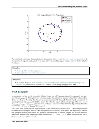


![scikit-learn user guide, Release 0.16.0
Regression criteria
If the target is a continuous value, then for node 𝑚, representing a region 𝑅 𝑚 with 𝑁 𝑚 observations, a common
criterion to minimise is the Mean Squared Error
𝑐 𝑚 =
1
𝑁 𝑚
∑︁
𝑖∈𝑁 𝑚
𝑦𝑖
𝐻(𝑋 𝑚) =
1
𝑁 𝑚
∑︁
𝑖∈𝑁 𝑚
(𝑦𝑖 − 𝑐 𝑚)2
References:
• http://en.wikipedia.org/wiki/Decision_tree_learning
• http://en.wikipedia.org/wiki/Predictive_analytics
• L. Breiman, J. Friedman, R. Olshen, and C. Stone. Classification and Regression Trees. Wadsworth,
Belmont, CA, 1984.
• J.R. Quinlan. C4. 5: programs for machine learning. Morgan Kaufmann, 1993.
• T. Hastie, R. Tibshirani and J. Friedman. Elements of Statistical Learning, Springer, 2009.
4.11 Ensemble methods
The goal of ensemble methods is to combine the predictions of several base estimators built with a given learning
algorithm in order to improve generalizability / robustness over a single estimator.
Two families of ensemble methods are usually distinguished:
• In averaging methods, the driving principle is to build several estimators independently and then to average
their predictions. On average, the combined estimator is usually better than any of the single base estimator
because its variance is reduced.
Examples: Bagging methods, Forests of randomized trees, ...
• By contrast, in boosting methods, base estimators are built sequentially and one tries to reduce the bias of the
combined estimator. The motivation is to combine several weak models to produce a powerful ensemble.
Examples: AdaBoost, Gradient Tree Boosting, ...
4.11.1 Bagging meta-estimator
In ensemble algorithms, bagging methods form a class of algorithms which build several instances of a black-box
estimator on random subsets of the original training set and then aggregate their individual predictions to form a final
prediction. These methods are used as a way to reduce the variance of a base estimator (e.g., a decision tree), by
introducing randomization into its construction procedure and then making an ensemble out of it. In many cases,
bagging methods constitute a very simple way to improve with respect to a single model, without making it necessary
to adapt the underlying base algorithm. As they provide a way to reduce overfitting, bagging methods work best with
strong and complex models (e.g., fully developed decision trees), in contrast with boosting methods which usually
work best with weak models (e.g., shallow decision trees).
Bagging methods come in many flavours but mostly differ from each other by the way they draw random subsets of
the training set:
• When random subsets of the dataset are drawn as random subsets of the samples, then this algorithm is known
as Pasting [B1999].
4.11. Ensemble methods 115](https://image.slidesharecdn.com/scikit-learn0-150409112902-conversion-gate01/85/Scikit-learn-0-16-0-user-guide-125-320.jpg)
![scikit-learn user guide, Release 0.16.0
• When samples are drawn with replacement, then the method is known as Bagging [B1996].
• When random subsets of the dataset are drawn as random subsets of the features, then the method is known as
Random Subspaces [H1998].
• Finally, when base estimators are built on subsets of both samples and features, then the method is known as
Random Patches [LG2012].
In scikit-learn, bagging methods are offered as a unified BaggingClassifier meta-estimator (resp.
BaggingRegressor), taking as input a user-specified base estimator along with parameters specifying the strategy
to draw random subsets. In particular, max_samples and max_features control the size of the subsets (in terms
of samples and features), while bootstrap and bootstrap_features control whether samples and features
are drawn with or without replacement. As an example, the snippet below illustrates how to instantiate a bagging
ensemble of KNeighborsClassifier base estimators, each built on random subsets of 50% of the samples and
50% of the features.
>>> from sklearn.ensemble import BaggingClassifier
>>> from sklearn.neighbors import KNeighborsClassifier
>>> bagging = BaggingClassifier(KNeighborsClassifier(),
... max_samples=0.5, max_features=0.5)
Examples:
• Single estimator versus bagging: bias-variance decomposition
References
4.11.2 Forests of randomized trees
The sklearn.ensemble module includes two averaging algorithms based on randomized decision trees: the Ran-
domForest algorithm and the Extra-Trees method. Both algorithms are perturb-and-combine techniques [B1998]
specifically designed for trees. This means a diverse set of classifiers is created by introducing randomness in the
classifier construction. The prediction of the ensemble is given as the averaged prediction of the individual classifiers.
As other classifiers, forest classifiers have to be fitted with two arrays: a sparse or dense array X of size [n_samples,
n_features] holding the training samples, and an array Y of size [n_samples] holding the target values (class
labels) for the training samples:
>>> from sklearn.ensemble import RandomForestClassifier
>>> X = [[0, 0], [1, 1]]
>>> Y = [0, 1]
>>> clf = RandomForestClassifier(n_estimators=10)
>>> clf = clf.fit(X, Y)
Like decision trees, forests of trees also extend to multi-output problems (if Y is an array of size [n_samples,
n_outputs]).
Random Forests
In random forests (see RandomForestClassifier and RandomForestRegressor classes), each tree in the
ensemble is built from a sample drawn with replacement (i.e., a bootstrap sample) from the training set. In addition,
when splitting a node during the construction of the tree, the split that is chosen is no longer the best split among all
features. Instead, the split that is picked is the best split among a random subset of the features. As a result of this
116 Chapter 4. Supervised learning](https://image.slidesharecdn.com/scikit-learn0-150409112902-conversion-gate01/85/Scikit-learn-0-16-0-user-guide-126-320.jpg)
![scikit-learn user guide, Release 0.16.0
randomness, the bias of the forest usually slightly increases (with respect to the bias of a single non-random tree) but,
due to averaging, its variance also decreases, usually more than compensating for the increase in bias, hence yielding
an overall better model.
In contrast to the original publication [B2001], the scikit-learn implementation combines classifiers by averaging their
probabilistic prediction, instead of letting each classifier vote for a single class.
Extremely Randomized Trees
In extremely randomized trees (see ExtraTreesClassifier and ExtraTreesRegressor classes), random-
ness goes one step further in the way splits are computed. As in random forests, a random subset of candidate features
is used, but instead of looking for the most discriminative thresholds, thresholds are drawn at random for each candi-
date feature and the best of these randomly-generated thresholds is picked as the splitting rule. This usually allows to
reduce the variance of the model a bit more, at the expense of a slightly greater increase in bias:
>>> from sklearn.cross_validation import cross_val_score
>>> from sklearn.datasets import make_blobs
>>> from sklearn.ensemble import RandomForestClassifier
>>> from sklearn.ensemble import ExtraTreesClassifier
>>> from sklearn.tree import DecisionTreeClassifier
>>> X, y = make_blobs(n_samples=10000, n_features=10, centers=100,
... random_state=0)
>>> clf = DecisionTreeClassifier(max_depth=None, min_samples_split=1,
... random_state=0)
>>> scores = cross_val_score(clf, X, y)
>>> scores.mean()
0.97...
>>> clf = RandomForestClassifier(n_estimators=10, max_depth=None,
... min_samples_split=1, random_state=0)
>>> scores = cross_val_score(clf, X, y)
>>> scores.mean()
0.999...
>>> clf = ExtraTreesClassifier(n_estimators=10, max_depth=None,
... min_samples_split=1, random_state=0)
>>> scores = cross_val_score(clf, X, y)
>>> scores.mean() > 0.999
True
Parameters
The main parameters to adjust when using these methods is n_estimators and max_features. The former
is the number of trees in the forest. The larger the better, but also the longer it will take to compute. In addition,
note that results will stop getting significantly better beyond a critical number of trees. The latter is the size of
the random subsets of features to consider when splitting a node. The lower the greater the reduction of variance,
but also the greater the increase in bias. Empirical good default values are max_features=n_features for
regression problems, and max_features=sqrt(n_features) for classification tasks (where n_features is
the number of features in the data). Good results are often achieved when setting max_depth=None in combination
with min_samples_split=1 (i.e., when fully developing the trees). Bear in mind though that these values are
usually not optimal, and might result in models that consume a lot of ram. The best parameter values should always be
cross-validated. In addition, note that in random forests, bootstrap samples are used by default (bootstrap=True)
while the default strategy for extra-trees is to use the whole dataset (bootstrap=False).
4.11. Ensemble methods 117](https://image.slidesharecdn.com/scikit-learn0-150409112902-conversion-gate01/85/Scikit-learn-0-16-0-user-guide-127-320.jpg)


![scikit-learn user guide, Release 0.16.0
Examples:
• Hashing feature transformation using Totally Random Trees
• Manifold learning on handwritten digits: Locally Linear Embedding, Isomap... compares non-linear
dimensionality reduction techniques on handwritten digits.
See also:
Manifold learning techniques can also be useful to derive non-linear representations of feature space, also these ap-
proaches focus also on dimensionality reduction.
4.11.3 AdaBoost
The module sklearn.ensemble includes the popular boosting algorithm AdaBoost, introduced in 1995 by Freund
and Schapire [FS1995].
The core principle of AdaBoost is to fit a sequence of weak learners (i.e., models that are only slightly better than
random guessing, such as small decision trees) on repeatedly modified versions of the data. The predictions from
all of them are then combined through a weighted majority vote (or sum) to produce the final prediction. The data
modifications at each so-called boosting iteration consist of applying weights 𝑤1, 𝑤2, ..., 𝑤 𝑁 to each of the training
samples. Initially, those weights are all set to 𝑤𝑖 = 1/𝑁, so that the first step simply trains a weak learner on the
original data. For each successive iteration, the sample weights are individually modified and the learning algorithm is
reapplied to the reweighted data. At a given step, those training examples that were incorrectly predicted by the boosted
model induced at the previous step have their weights increased, whereas the weights are decreased for those that were
predicted correctly. As iterations proceed, examples that are difficult to predict receive ever-increasing influence. Each
subsequent weak learner is thereby forced to concentrate on the examples that are missed by the previous ones in the
sequence [HTF].
AdaBoost can be used both for classification and regression problems:
120 Chapter 4. Supervised learning](https://image.slidesharecdn.com/scikit-learn0-150409112902-conversion-gate01/85/Scikit-learn-0-16-0-user-guide-130-320.jpg)
![scikit-learn user guide, Release 0.16.0
• For multi-class classification, AdaBoostClassifier implements AdaBoost-SAMME and AdaBoost-
SAMME.R [ZZRH2009].
• For regression, AdaBoostRegressor implements AdaBoost.R2 [D1997].
Usage
The following example shows how to fit an AdaBoost classifier with 100 weak learners:
>>> from sklearn.cross_validation import cross_val_score
>>> from sklearn.datasets import load_iris
>>> from sklearn.ensemble import AdaBoostClassifier
>>> iris = load_iris()
>>> clf = AdaBoostClassifier(n_estimators=100)
>>> scores = cross_val_score(clf, iris.data, iris.target)
>>> scores.mean()
0.9...
The number of weak learners is controlled by the parameter n_estimators. The learning_rate parameter
controls the contribution of the weak learners in the final combination. By default, weak learners are decision stumps.
Different weak learners can be specified through the base_estimator parameter. The main parameters to tune to
obtain good results are n_estimators and the complexity of the base estimators (e.g., its depth max_depth or
minimum required number of samples at a leaf min_samples_leaf in case of decision trees).
Examples:
• Discrete versus Real AdaBoost compares the classification error of a decision stump, decision tree, and a
boosted decision stump using AdaBoost-SAMME and AdaBoost-SAMME.R.
• Multi-class AdaBoosted Decision Trees shows the performance of AdaBoost-SAMME and AdaBoost-
SAMME.R on a multi-class problem.
• Two-class AdaBoost shows the decision boundary and decision function values for a non-linearly separable
two-class problem using AdaBoost-SAMME.
• Decision Tree Regression with AdaBoost demonstrates regression with the AdaBoost.R2 algorithm.
References
4.11.4 Gradient Tree Boosting
Gradient Tree Boosting or Gradient Boosted Regression Trees (GBRT) is a generalization of boosting to arbitrary
differentiable loss functions. GBRT is an accurate and effective off-the-shelf procedure that can be used for both
regression and classification problems. Gradient Tree Boosting models are used in a variety of areas including Web
search ranking and ecology.
The advantages of GBRT are:
• Natural handling of data of mixed type (= heterogeneous features)
• Predictive power
• Robustness to outliers in output space (via robust loss functions)
The disadvantages of GBRT are:
4.11. Ensemble methods 121](https://image.slidesharecdn.com/scikit-learn0-150409112902-conversion-gate01/85/Scikit-learn-0-16-0-user-guide-131-320.jpg)
![scikit-learn user guide, Release 0.16.0
• Scalability, due to the sequential nature of boosting it can hardly be parallelized.
The module sklearn.ensemble provides methods for both classification and regression via gradient boosted
regression trees.
Classification
GradientBoostingClassifier supports both binary and multi-class classification. The following example
shows how to fit a gradient boosting classifier with 100 decision stumps as weak learners:
>>> from sklearn.datasets import make_hastie_10_2
>>> from sklearn.ensemble import GradientBoostingClassifier
>>> X, y = make_hastie_10_2(random_state=0)
>>> X_train, X_test = X[:2000], X[2000:]
>>> y_train, y_test = y[:2000], y[2000:]
>>> clf = GradientBoostingClassifier(n_estimators=100, learning_rate=1.0,
... max_depth=1, random_state=0).fit(X_train, y_train)
>>> clf.score(X_test, y_test)
0.913...
The number of weak learners (i.e. regression trees) is controlled by the parameter n_estimators; The size of each
tree can be controlled either by setting the tree depth via max_depth or by setting the number of leaf nodes via
max_leaf_nodes. The learning_rate is a hyper-parameter in the range (0.0, 1.0] that controls overfitting via
shrinkage .
Note: Classification with more than 2 classes requires the induction of n_classes regression trees at each
at each iteration, thus, the total number of induced trees equals n_classes * n_estimators. For datasets
with a large number of classes we strongly recommend to use RandomForestClassifier as an alternative to
GradientBoostingClassifier .
Regression
GradientBoostingRegressor supports a number of different loss functions for regression which can be speci-
fied via the argument loss; the default loss function for regression is least squares (’ls’).
>>> import numpy as np
>>> from sklearn.metrics import mean_squared_error
>>> from sklearn.datasets import make_friedman1
>>> from sklearn.ensemble import GradientBoostingRegressor
>>> X, y = make_friedman1(n_samples=1200, random_state=0, noise=1.0)
>>> X_train, X_test = X[:200], X[200:]
>>> y_train, y_test = y[:200], y[200:]
>>> est = GradientBoostingRegressor(n_estimators=100, learning_rate=0.1,
... max_depth=1, random_state=0, loss='ls').fit(X_train, y_train)
>>> mean_squared_error(y_test, est.predict(X_test))
5.00...
The figure below shows the results of applying GradientBoostingRegressor with least squares loss and 500
base learners to the Boston house price dataset (sklearn.datasets.load_boston). The plot on the left shows
the train and test error at each iteration. The train error at each iteration is stored in the train_score_ attribute
of the gradient boosting model. The test error at each iterations can be obtained via the staged_predict method
which returns a generator that yields the predictions at each stage. Plots like these can be used to determine the optimal
122 Chapter 4. Supervised learning](https://image.slidesharecdn.com/scikit-learn0-150409112902-conversion-gate01/85/Scikit-learn-0-16-0-user-guide-132-320.jpg)
![scikit-learn user guide, Release 0.16.0
number of trees (i.e. n_estimators) by early stopping. The plot on the right shows the feature importances which
can be obtained via the feature_importances_ property.
Examples:
• Gradient Boosting regression
• Gradient Boosting Out-of-Bag estimates
Fitting additional weak-learners
Both GradientBoostingRegressor and GradientBoostingClassifier support warm_start=True
which allows you to add more estimators to an already fitted model.
>>> _ = est.set_params(n_estimators=200, warm_start=True) # set warm_start and new nr of trees
>>> _ = est.fit(X_train, y_train) # fit additional 100 trees to est
>>> mean_squared_error(y_test, est.predict(X_test))
3.84...
Controlling the tree size
The size of the regression tree base learners defines the level of variable interactions that can be captured by the
gradient boosting model. In general, a tree of depth h can capture interactions of order h . There are two ways in
which the size of the individual regression trees can be controlled.
If you specify max_depth=h then complete binary trees of depth h will be grown. Such trees will have (at most)
2**h leaf nodes and 2**h - 1 split nodes.
Alternatively, you can control the tree size by specifying the number of leaf nodes via the parameter
max_leaf_nodes. In this case, trees will be grown using best-first search where nodes with the highest improve-
ment in impurity will be expanded first. A tree with max_leaf_nodes=k has k - 1 split nodes and thus can
model interactions of up to order max_leaf_nodes - 1 .
We found that max_leaf_nodes=k gives comparable results to max_depth=k-1 but is significantly faster to
train at the expense of a slightly higher training error. The parameter max_leaf_nodes corresponds to the variable
J in the chapter on gradient boosting in [F2001] and is related to the parameter interaction.depth in R’s gbm
package where max_leaf_nodes == interaction.depth + 1 .
4.11. Ensemble methods 123](https://image.slidesharecdn.com/scikit-learn0-150409112902-conversion-gate01/85/Scikit-learn-0-16-0-user-guide-133-320.jpg)

![scikit-learn user guide, Release 0.16.0
– Least squares (’ls’): The natural choice for regression due to its superior computational properties. The
initial model is given by the mean of the target values.
– Least absolute deviation (’lad’): A robust loss function for regression. The initial model is given by the
median of the target values.
– Huber (’huber’): Another robust loss function that combines least squares and least absolute deviation;
use alpha to control the sensitivity with regards to outliers (see [F2001] for more details).
– Quantile (’quantile’): A loss function for quantile regression. Use 0 < alpha < 1 to specify the
quantile. This loss function can be used to create prediction intervals (see Prediction Intervals for Gradient
Boosting Regression).
• Classification
– Binomial deviance (’deviance’): The negative binomial log-likelihood loss function for binary classi-
fication (provides probability estimates). The initial model is given by the log odds-ratio.
– Multinomial deviance (’deviance’): The negative multinomial log-likelihood loss function for multi-
class classification with n_classes mutually exclusive classes. It provides probability estimates. The
initial model is given by the prior probability of each class. At each iteration n_classes regression trees
have to be constructed which makes GBRT rather inefficient for data sets with a large number of classes.
– Exponential loss (’exponential’): The same loss function as AdaBoostClassifier. Less robust
to mislabeled examples than ’deviance’; can only be used for binary classification.
Regularization
Shrinkage
[F2001] proposed a simple regularization strategy that scales the contribution of each weak learner by a factor 𝜈:
𝐹 𝑚(𝑥) = 𝐹 𝑚−1(𝑥) + 𝜈𝛾 𝑚ℎ 𝑚(𝑥)
The parameter 𝜈 is also called the learning rate because it scales the step length the the gradient descent procedure; it
can be set via the learning_rate parameter.
The parameter learning_rate strongly interacts with the parameter n_estimators, the number of weak learn-
ers to fit. Smaller values of learning_rate require larger numbers of weak learners to maintain a constant training
error. Empirical evidence suggests that small values of learning_rate favor better test error. [HTF2009] recom-
mend to set the learning rate to a small constant (e.g. learning_rate <= 0.1) and choose n_estimators by
early stopping. For a more detailed discussion of the interaction between learning_rate and n_estimators
see [R2007].
Subsampling
[F1999] proposed stochastic gradient boosting, which combines gradient boosting with bootstrap averaging (bagging).
At each iteration the base classifier is trained on a fraction subsample of the available training data. The subsample
is drawn without replacement. A typical value of subsample is 0.5.
The figure below illustrates the effect of shrinkage and subsampling on the goodness-of-fit of the model. We can
clearly see that shrinkage outperforms no-shrinkage. Subsampling with shrinkage can further increase the accuracy of
the model. Subsampling without shrinkage, on the other hand, does poorly.
Another strategy to reduce the variance is by subsampling the features analogous to the random splits in
RandomForestClassifier . The number of subsampled features can be controlled via the max_features
parameter.
4.11. Ensemble methods 125](https://image.slidesharecdn.com/scikit-learn0-150409112902-conversion-gate01/85/Scikit-learn-0-16-0-user-guide-135-320.jpg)
![scikit-learn user guide, Release 0.16.0
Note: Using a small max_features value can significantly decrease the runtime.
Stochastic gradient boosting allows to compute out-of-bag estimates of the test deviance by computing the improve-
ment in deviance on the examples that are not included in the bootstrap sample (i.e. the out-of-bag examples). The
improvements are stored in the attribute oob_improvement_. oob_improvement_[i] holds the improvement
in terms of the loss on the OOB samples if you add the i-th stage to the current predictions. Out-of-bag estimates can
be used for model selection, for example to determine the optimal number of iterations. OOB estimates are usually
very pessimistic thus we recommend to use cross-validation instead and only use OOB if cross-validation is too time
consuming.
Examples:
• Gradient Boosting regularization
• Gradient Boosting Out-of-Bag estimates
Interpretation
Individual decision trees can be interpreted easily by simply visualizing the tree structure. Gradient boosting models,
however, comprise hundreds of regression trees thus they cannot be easily interpreted by visual inspection of the
individual trees. Fortunately, a number of techniques have been proposed to summarize and interpret gradient boosting
models.
Feature importance
Often features do not contribute equally to predict the target response; in many situations the majority of the features
are in fact irrelevant. When interpreting a model, the first question usually is: what are those important features and
how do they contributing in predicting the target response?
126 Chapter 4. Supervised learning](https://image.slidesharecdn.com/scikit-learn0-150409112902-conversion-gate01/85/Scikit-learn-0-16-0-user-guide-136-320.jpg)

![scikit-learn user guide, Release 0.16.0
>>> features = [0, 1, (0, 1)]
>>> fig, axs = plot_partial_dependence(clf, X, features)
For multi-class models, you need to set the class label for which the PDPs should be created via the label argument:
>>> from sklearn.datasets import load_iris
>>> iris = load_iris()
>>> mc_clf = GradientBoostingClassifier(n_estimators=10,
... max_depth=1).fit(iris.data, iris.target)
>>> features = [3, 2, (3, 2)]
>>> fig, axs = plot_partial_dependence(mc_clf, X, features, label=0)
If you need the raw values of the partial dependence function rather than the plots you can use the
partial_dependence function:
>>> from sklearn.ensemble.partial_dependence import partial_dependence
>>> pdp, axes = partial_dependence(clf, [0], X=X)
>>> pdp
array([[ 2.46643157, 2.46643157, ...
>>> axes
[array([-1.62497054, -1.59201391, ...
The function requires either the argument grid which specifies the values of the target features on which the partial
dependence function should be evaluated or the argument X which is a convenience mode for automatically creating
grid from the training data. If X is given, the axes value returned by the function gives the axis for each target
feature.
For each value of the ‘target’ features in the grid the partial dependence function need to marginalize the predictions
of a tree over all possible values of the ‘complement’ features. In decision trees this function can be evaluated effi-
ciently without reference to the training data. For each grid point a weighted tree traversal is performed: if a split node
involves a ‘target’ feature, the corresponding left or right branch is followed, otherwise both branches are followed,
each branch is weighted by the fraction of training samples that entered that branch. Finally, the partial dependence
is given by a weighted average of all visited leaves. For tree ensembles the results of each individual tree are again
128 Chapter 4. Supervised learning](https://image.slidesharecdn.com/scikit-learn0-150409112902-conversion-gate01/85/Scikit-learn-0-16-0-user-guide-138-320.jpg)

![scikit-learn user guide, Release 0.16.0
Warning: At present, no metric in sklearn.metrics supports the multioutput-multiclass classification task.
4.12.1 Multilabel classification format
In multilabel learning, the joint set of binary classification tasks is expressed with label binary indicator array: each
sample is one row of a 2d array of shape (n_samples, n_classes) with binary values: the one, i.e. the non zero elements,
corresponds to the subset of labels. An array such as np.array([[1, 0, 0], [0, 1, 1], [0, 0, 0]])
represents label 0 in the first sample, labels 1 and 2 in the second sample, and no labels in the third sample.
Producing multilabel data as a list of sets of labels may be more intuitive. The transformer MultiLabelBinarizer
will convert between a collection of collections of labels and the indicator format.
>>> from sklearn.datasets import make_multilabel_classification
>>> from sklearn.preprocessing import MultiLabelBinarizer
>>> X, Y = make_multilabel_classification(n_samples=5, random_state=0,
... return_indicator=False)
>>> Y
[[2, 3, 4], [2], [0, 1, 3], [0, 1, 2, 3, 4], [0, 1, 2]]
>>> MultiLabelBinarizer().fit_transform(Y)
array([[0, 0, 1, 1, 1],
[0, 0, 1, 0, 0],
[1, 1, 0, 1, 0],
[1, 1, 1, 1, 1],
[1, 1, 1, 0, 0]])
4.12.2 One-Vs-The-Rest
This strategy, also known as one-vs-all, is implemented in OneVsRestClassifier. The strategy consists in
fitting one classifier per class. For each classifier, the class is fitted against all the other classes. In addition to its
computational efficiency (only n_classes classifiers are needed), one advantage of this approach is its interpretability.
Since each class is represented by one and one classifier only, it is possible to gain knowledge about the class by
inspecting its corresponding classifier. This is the most commonly used strategy and is a fair default choice.
Multiclass learning
Below is an example of multiclass learning using OvR:
>>> from sklearn import datasets
>>> from sklearn.multiclass import OneVsRestClassifier
>>> from sklearn.svm import LinearSVC
>>> iris = datasets.load_iris()
>>> X, y = iris.data, iris.target
>>> OneVsRestClassifier(LinearSVC(random_state=0)).fit(X, y).predict(X)
array([0, 0, 0, 0, 0, 0, 0, 0, 0, 0, 0, 0, 0, 0, 0, 0, 0, 0, 0, 0, 0, 0, 0,
0, 0, 0, 0, 0, 0, 0, 0, 0, 0, 0, 0, 0, 0, 0, 0, 0, 0, 0, 0, 0, 0, 0,
0, 0, 0, 0, 1, 1, 1, 1, 1, 1, 1, 1, 1, 1, 1, 1, 1, 1, 1, 1, 1, 1, 1,
1, 2, 1, 1, 1, 1, 1, 1, 1, 1, 1, 1, 1, 1, 2, 2, 1, 1, 1, 1, 1, 1, 1,
1, 1, 1, 1, 1, 1, 1, 1, 2, 2, 2, 2, 2, 2, 2, 2, 2, 2, 2, 2, 2, 2, 2,
2, 2, 2, 2, 2, 2, 2, 2, 2, 2, 2, 2, 2, 2, 1, 2, 2, 2, 1, 2, 2, 2, 2,
2, 2, 2, 2, 2, 2, 2, 2, 2, 2, 2, 2])
130 Chapter 4. Supervised learning](https://image.slidesharecdn.com/scikit-learn0-150409112902-conversion-gate01/85/Scikit-learn-0-16-0-user-guide-140-320.jpg)
![scikit-learn user guide, Release 0.16.0
Multilabel learning
OneVsRestClassifier also supports multilabel classification. To use this feature, feed the classifier an indicator
matrix, in which cell [i, j] indicates the presence of label j in sample i.
Examples:
• Multilabel classification
4.12.3 One-Vs-One
OneVsOneClassifier constructs one classifier per pair of classes. At prediction time, the class which received
the most votes is selected. In the event of a tie (among two classes with an equal number of votes), it selects the class
with the highest aggregate classification confidence by summing over the pair-wise classification confidence levels
computed by the underlying binary classifiers.
Since it requires to fit n_classes * (n_classes - 1) / 2 classifiers, this method is usually slower than
one-vs-the-rest, due to its O(n_classes^2) complexity. However, this method may be advantageous for algorithms
such as kernel algorithms which don’t scale well with n_samples. This is because each individual learning problem
only involves a small subset of the data whereas, with one-vs-the-rest, the complete dataset is used n_classes times.
Multiclass learning
Below is an example of multiclass learning using OvO:
>>> from sklearn import datasets
>>> from sklearn.multiclass import OneVsOneClassifier
>>> from sklearn.svm import LinearSVC
4.12. Multiclass and multilabel algorithms 131](https://image.slidesharecdn.com/scikit-learn0-150409112902-conversion-gate01/85/Scikit-learn-0-16-0-user-guide-141-320.jpg)
![scikit-learn user guide, Release 0.16.0
>>> iris = datasets.load_iris()
>>> X, y = iris.data, iris.target
>>> OneVsOneClassifier(LinearSVC(random_state=0)).fit(X, y).predict(X)
array([0, 0, 0, 0, 0, 0, 0, 0, 0, 0, 0, 0, 0, 0, 0, 0, 0, 0, 0, 0, 0, 0, 0,
0, 0, 0, 0, 0, 0, 0, 0, 0, 0, 0, 0, 0, 0, 0, 0, 0, 0, 0, 0, 0, 0, 0,
0, 0, 0, 0, 1, 1, 1, 1, 1, 1, 1, 1, 1, 1, 1, 1, 1, 1, 1, 1, 1, 1, 1,
1, 2, 1, 2, 1, 1, 1, 1, 1, 1, 1, 1, 1, 1, 2, 1, 1, 1, 1, 1, 1, 1, 1,
1, 1, 1, 1, 1, 1, 1, 1, 2, 2, 2, 2, 2, 2, 2, 2, 2, 2, 2, 2, 2, 2, 2,
2, 2, 2, 2, 2, 2, 2, 2, 2, 2, 2, 2, 2, 2, 2, 2, 2, 2, 2, 2, 2, 2, 2,
2, 2, 2, 2, 2, 2, 2, 2, 2, 2, 2, 2])
References:
4.12.4 Error-Correcting Output-Codes
Output-code based strategies are fairly different from one-vs-the-rest and one-vs-one. With these strategies, each class
is represented in a euclidean space, where each dimension can only be 0 or 1. Another way to put it is that each class
is represented by a binary code (an array of 0 and 1). The matrix which keeps track of the location/code of each class
is called the code book. The code size is the dimensionality of the aforementioned space. Intuitively, each class should
be represented by a code as unique as possible and a good code book should be designed to optimize classification
accuracy. In this implementation, we simply use a randomly-generated code book as advocated in 7
although more
elaborate methods may be added in the future.
At fitting time, one binary classifier per bit in the code book is fitted. At prediction time, the classifiers are used to
project new points in the class space and the class closest to the points is chosen.
In OutputCodeClassifier, the code_size attribute allows the user to control the number of classifiers which
will be used. It is a percentage of the total number of classes.
A number between 0 and 1 will require fewer classifiers than one-vs-the-rest. In theory, log2(n_classes) /
n_classes is sufficient to represent each class unambiguously. However, in practice, it may not lead to good
accuracy since log2(n_classes) is much smaller than n_classes.
A number greater than than 1 will require more classifiers than one-vs-the-rest. In this case, some classifiers will in
theory correct for the mistakes made by other classifiers, hence the name “error-correcting”. In practice, however, this
may not happen as classifier mistakes will typically be correlated. The error-correcting output codes have a similar
effect to bagging.
Multiclass learning
Below is an example of multiclass learning using Output-Codes:
>>> from sklearn import datasets
>>> from sklearn.multiclass import OutputCodeClassifier
>>> from sklearn.svm import LinearSVC
>>> iris = datasets.load_iris()
>>> X, y = iris.data, iris.target
>>> clf = OutputCodeClassifier(LinearSVC(random_state=0),
... code_size=2, random_state=0)
>>> clf.fit(X, y).predict(X)
array([0, 0, 0, 0, 0, 0, 0, 0, 0, 0, 0, 0, 0, 0, 0, 0, 0, 0, 0, 0, 0, 0, 0,
0, 0, 0, 0, 0, 0, 0, 0, 0, 0, 0, 0, 0, 0, 0, 0, 0, 0, 0, 0, 0, 0, 0,
7 “The error coding method and PICTs”, James G., Hastie T., Journal of Computational and Graphical statistics 7, 1998.
132 Chapter 4. Supervised learning](https://image.slidesharecdn.com/scikit-learn0-150409112902-conversion-gate01/85/Scikit-learn-0-16-0-user-guide-142-320.jpg)
![scikit-learn user guide, Release 0.16.0
0, 0, 0, 0, 1, 1, 1, 1, 1, 1, 2, 1, 1, 1, 1, 1, 1, 1, 1, 1, 2, 1, 1,
1, 2, 1, 1, 1, 1, 1, 1, 2, 1, 1, 1, 1, 1, 2, 2, 2, 1, 1, 1, 1, 1, 1,
1, 1, 1, 1, 1, 1, 1, 1, 2, 2, 2, 2, 2, 2, 2, 2, 2, 2, 2, 2, 2, 2, 2,
2, 2, 2, 2, 1, 2, 2, 2, 2, 2, 2, 2, 2, 2, 1, 2, 2, 2, 1, 1, 2, 2, 2,
2, 2, 2, 2, 2, 2, 2, 2, 2, 2, 2, 2])
References:
4.13 Feature selection
The classes in the sklearn.feature_selection module can be used for feature selection/dimensionality re-
duction on sample sets, either to improve estimators’ accuracy scores or to boost their performance on very high-
dimensional datasets.
4.13.1 Removing features with low variance
VarianceThreshold is a simple baseline approach to feature selection. It removes all features whose variance
doesn’t meet some threshold. By default, it removes all zero-variance features, i.e. features that have the same value
in all samples.
As an example, suppose that we have a dataset with boolean features, and we want to remove all features that are
either one or zero (on or off) in more than 80% of the samples. Boolean features are Bernoulli random variables, and
the variance of such variables is given by
Var[𝑋] = 𝑝(1 − 𝑝)
so we can select using the threshold .8 * (1 - .8):
>>> from sklearn.feature_selection import VarianceThreshold
>>> X = [[0, 0, 1], [0, 1, 0], [1, 0, 0], [0, 1, 1], [0, 1, 0], [0, 1, 1]]
>>> sel = VarianceThreshold(threshold=(.8 * (1 - .8)))
>>> sel.fit_transform(X)
array([[0, 1],
[1, 0],
[0, 0],
[1, 1],
[1, 0],
[1, 1]])
As expected, VarianceThreshold has removed the first column, which has a probability 𝑝 = 5/6 > .8 of
containing a zero.
4.13.2 Univariate feature selection
Univariate feature selection works by selecting the best features based on univariate statistical tests. It can be seen
as a preprocessing step to an estimator. Scikit-learn exposes feature selection routines as objects that implement the
transform method:
• SelectKBest removes all but the 𝑘 highest scoring features
• SelectPercentile removes all but a user-specified highest scoring percentage of features
4.13. Feature selection 133](https://image.slidesharecdn.com/scikit-learn0-150409112902-conversion-gate01/85/Scikit-learn-0-16-0-user-guide-143-320.jpg)

![scikit-learn user guide, Release 0.16.0
4.13.4 L1-based feature selection
Selecting non-zero coefficients
Linear models penalized with the L1 norm have sparse solutions: many of their estimated coefficients are
zero. When the goal is to reduce the dimensionality of the data to use with another classifier, they expose
a transform method to select the non-zero coefficient. In particular, sparse estimators useful for this pur-
pose are the linear_model.Lasso for regression, and of linear_model.LogisticRegression and
svm.LinearSVC for classification:
>>> from sklearn.svm import LinearSVC
>>> from sklearn.datasets import load_iris
>>> iris = load_iris()
>>> X, y = iris.data, iris.target
>>> X.shape
(150, 4)
>>> X_new = LinearSVC(C=0.01, penalty="l1", dual=False).fit_transform(X, y)
>>> X_new.shape
(150, 3)
With SVMs and logistic-regression, the parameter C controls the sparsity: the smaller C the fewer features selected.
With Lasso, the higher the alpha parameter, the fewer features selected.
Examples:
• Classification of text documents using sparse features: Comparison of different algorithms for document
classification including L1-based feature selection.
L1-recovery and compressive sensing
For a good choice of alpha, the Lasso can fully recover the exact set of non-zero variables using only few obser-
vations, provided certain specific conditions are met. In particular, the number of samples should be “sufficiently
large”, or L1 models will perform at random, where “sufficiently large” depends on the number of non-zero co-
efficients, the logarithm of the number of features, the amount of noise, the smallest absolute value of non-zero
coefficients, and the structure of the design matrix X. In addition, the design matrix must display certain specific
properties, such as not being too correlated.
There is no general rule to select an alpha parameter for recovery of non-zero coefficients. It can by set by
cross-validation (LassoCV or LassoLarsCV), though this may lead to under-penalized models: including a
small number of non-relevant variables is not detrimental to prediction score. BIC (LassoLarsIC) tends, on
the opposite, to set high values of alpha.
Reference Richard G. Baraniuk “Compressive Sensing”, IEEE Signal Processing Magazine [120] July 2007
http://dsp.rice.edu/files/cs/baraniukCSlecture07.pdf
Randomized sparse models
The limitation of L1-based sparse models is that faced with a group of very correlated features, they will select only
one. To mitigate this problem, it is possible to use randomization techniques, reestimating the sparse model many
times perturbing the design matrix or sub-sampling data and counting how many times a given regressor is selected.
RandomizedLasso implements this strategy for regression settings, using the Lasso, while
RandomizedLogisticRegression uses the logistic regression and is suitable for classification tasks. To
get a full path of stability scores you can use lasso_stability_path.
4.13. Feature selection 135](https://image.slidesharecdn.com/scikit-learn0-150409112902-conversion-gate01/85/Scikit-learn-0-16-0-user-guide-145-320.jpg)
![scikit-learn user guide, Release 0.16.0
Note that for randomized sparse models to be more powerful than standard F statistics at detecting non-zero features,
the ground truth model should be sparse, in other words, there should be only a small fraction of features non zero.
Examples:
• Sparse recovery: feature selection for sparse linear models: An example comparing different feature
selection approaches and discussing in which situation each approach is to be favored.
References:
• N. Meinshausen, P. Buhlmann, “Stability selection”, Journal of the Royal Statistical Society, 72 (2010)
http://arxiv.org/pdf/0809.2932
• F. Bach, “Model-Consistent Sparse Estimation through the Bootstrap” http://hal.inria.fr/hal-00354771/
4.13.5 Tree-based feature selection
Tree-based estimators (see the sklearn.tree module and forest of trees in the sklearn.ensemble module)
can be used to compute feature importances, which in turn can be used to discard irrelevant features:
>>> from sklearn.ensemble import ExtraTreesClassifier
>>> from sklearn.datasets import load_iris
>>> iris = load_iris()
>>> X, y = iris.data, iris.target
>>> X.shape
(150, 4)
>>> clf = ExtraTreesClassifier()
>>> X_new = clf.fit(X, y).transform(X)
>>> clf.feature_importances_
array([ 0.04..., 0.05..., 0.4..., 0.4...])
>>> X_new.shape
(150, 2)
136 Chapter 4. Supervised learning](https://image.slidesharecdn.com/scikit-learn0-150409112902-conversion-gate01/85/Scikit-learn-0-16-0-user-guide-146-320.jpg)
![scikit-learn user guide, Release 0.16.0
Examples:
• Feature importances with forests of trees: example on synthetic data showing the recovery of the actually
meaningful features.
• Pixel importances with a parallel forest of trees: example on face recognition data.
4.13.6 Feature selection as part of a pipeline
Feature selection is usually used as a pre-processing step before doing the actual learning. The recommended way to
do this in scikit-learn is to use a sklearn.pipeline.Pipeline:
clf = Pipeline([
('feature_selection', LinearSVC(penalty="l1")),
('classification', RandomForestClassifier())
])
clf.fit(X, y)
In this snippet we make use of a sklearn.svm.LinearSVC to evaluate feature importances and select the
most relevant features. Then, a sklearn.ensemble.RandomForestClassifier is trained on the trans-
formed output, i.e. using only relevant features. You can perform similar operations with the other feature
selection methods and also classifiers that provide a way to evaluate feature importances of course. See the
sklearn.pipeline.Pipeline examples for more details.
4.14 Semi-Supervised
Semi-supervised learning is a situation in which in your training data some of the samples are not labeled. The semi-
supervised estimators in sklearn.semi_supervised are able to make use of this additional unlabeled data to
better capture the shape of the underlying data distribution and generalize better to new samples. These algorithms
can perform well when we have a very small amount of labeled points and a large amount of unlabeled points.
Unlabeled entries in y
It is important to assign an identifier to unlabeled points along with the labeled data when training the model
with the fit method. The identifier that this implementation uses is the integer value −1.
4.14.1 Label Propagation
Label propagation denotes a few variations of semi-supervised graph inference algorithms.
A few features available in this model:
• Can be used for classification and regression tasks
• Kernel methods to project data into alternate dimensional spaces
scikit-learn provides two label propagation models: LabelPropagation and LabelSpreading. Both work by
constructing a similarity graph over all items in the input dataset.
LabelPropagation and LabelSpreading differ in modifications to the similarity matrix that graph and the
clamping effect on the label distributions. Clamping allows the algorithm to change the weight of the true ground
labeled data to some degree. The LabelPropagation algorithm performs hard clamping of input labels, which
4.14. Semi-Supervised 137](https://image.slidesharecdn.com/scikit-learn0-150409112902-conversion-gate01/85/Scikit-learn-0-16-0-user-guide-147-320.jpg)
![scikit-learn user guide, Release 0.16.0
Fig. 4.1: An illustration of label-propagation: the structure of unlabeled observations is consistent with the class
structure, and thus the class label can be propagated to the unlabeled observations of the training set.
means 𝛼 = 1. This clamping factor can be relaxed, to say 𝛼 = 0.8, which means that we will always retain 80 percent
of our original label distribution, but the algorithm gets to change it’s confidence of the distribution within 20 percent.
LabelPropagation uses the raw similarity matrix constructed from the data with no modifications. In contrast,
LabelSpreading minimizes a loss function that has regularization properties, as such it is often more robust to
noise. The algorithm iterates on a modified version of the original graph and normalizes the edge weights by computing
the normalized graph Laplacian matrix. This procedure is also used in Spectral clustering.
Label propagation models have two built-in kernel methods. Choice of kernel effects both scalability and performance
of the algorithms. The following are available:
• rbf (exp(−𝛾|𝑥 − 𝑦|2
), 𝛾 > 0). 𝛾 is specified by keyword gamma.
• knn (1[𝑥′
∈ 𝑘𝑁 𝑁(𝑥)]). 𝑘 is specified by keyword n_neighbors.
The RBF kernel will produce a fully connected graph which is represented in memory by a dense matrix. This matrix
may be very large and combined with the cost of performing a full matrix multiplication calculation for each iteration
of the algorithm can lead to prohibitively long running times. On the other hand, the KNN kernel will produce a much
more memory-friendly sparse matrix which can drastically reduce running times.
Examples
• Decision boundary of label propagation versus SVM on the Iris dataset
• Label Propagation learning a complex structure
• Label Propagation digits active learning
References
[1] Yoshua Bengio, Olivier Delalleau, Nicolas Le Roux. In Semi-Supervised Learning (2006), pp. 193-216
[2] Olivier Delalleau, Yoshua Bengio, Nicolas Le Roux. Efficient Non-Parametric Function Induction in Semi-
Supervised Learning. AISTAT 2005 http://research.microsoft.com/en-us/people/nicolasl/efficient_ssl.pdf
4.15 Isotonic regression
The class IsotonicRegression fits a non-decreasing function to data. It solves the following problem:
minimize
∑︀
𝑖 𝑤𝑖(𝑦𝑖 − ˆ𝑦𝑖)2
138 Chapter 4. Supervised learning](https://image.slidesharecdn.com/scikit-learn0-150409112902-conversion-gate01/85/Scikit-learn-0-16-0-user-guide-148-320.jpg)


![scikit-learn user guide, Release 0.16.0
• GaussianNB tends to push probabilties to 0 or 1 (note the counts in the histograms). This is mainly because
it makes the assumption that features are conditionally independent given the class, which is not the case in this
dataset which contains 2 redundant features.
• RandomForestClassifier shows the opposite behavior: the histograms show peaks at approximately
0.2 and 0.9 probability, while probabilities close to 0 or 1 are very rare. An explanation for this is given by
Niculescu-Mizil and Caruana [4]: “Methods such as bagging and random forests that average predictions from
a base set of models can have difficulty making predictions near 0 and 1 because variance in the underlying base
models will bias predictions that should be near zero or one away from these values. Because predictions are
restricted to the interval [0,1], errors caused by variance tend to be one-sided near zero and one. For example,
if a model should predict p = 0 for a case, the only way bagging can achieve this is if all bagged trees predict
zero. If we add noise to the trees that bagging is averaging over, this noise will cause some trees to predict
values larger than 0 for this case, thus moving the average prediction of the bagged ensemble away from 0. We
observe this effect most strongly with random forests because the base-level trees trained with random forests
have relatively high variance due to feature subseting.” As a result, the calibration curve shows a characteristic
sigmoid shape, indicating that the classifier could trust its “intuition” more and return probabilties closer to 0 or
1 typically.
• Linear Support Vector Classification (LinearSVC) shows an even more sigmoid curve as the RandomForest-
Classifier, which is typical for maximum-margin methods (compare Niculescu-Mizil and Caruana [4]), which
focus on hard samples that are close to the decision boundary (the support vectors).
Two approaches for performing calibration of probabilistic predictions are provided: a parametric approach based on
Platt’s sigmoid model and a non-parametric approach based on isotonic regression (sklearn.isotonic). Proba-
bility calibration should be done on new data not used for model fitting. The class CalibratedClassifierCV
uses a cross-validation generator and estimates for each split the model parameter on the train samples and the cali-
bration of the test samples. The probabilities predicted for the folds are then averaged. Already fitted classifiers can
be calibrated by CalibratedClassifierCV via the paramter cv=”prefit”. In this case, the user has to take care
manually that data for model fitting and calibration are disjoint.
The following images demonstrate the benefit of probability calibration. The first image present a dataset with 2
classes and 3 blobs of data. The blob in the middle contains random samples of each class. The probability for the
samples in this blob should be 0.5.
The following image shows on the data above the estimated probability using a Gaussian naive Bayes classifier without
calibration, with a sigmoid calibration and with a non-parametric isotonic calibration. One can observe that the non-
parametric model provides the most accurate probability estimates for samples in the middle, i.e., 0.5.
The following experiment is performed on an artificial dataset for binary classification with 100.000 samples (1.000
of them are used for model fitting) with 20 features. Of the 20 features, only 2 are informative and 10 are redundant.
The figure shows the estimated probabilities obtained with logistic regression, a linear support-vector classifier (SVC),
and linear SVC with both isotonic calibration and sigmoid calibration. The calibration performance is evaluated with
Brier score brier_score_loss, reported in the legend (the smaller the better).
One can observe here that logistic regression is well calibrated as its curve is nearly diagonal. Linear SVC’s calibration
curve has a sigmoid curve, which is typical for an under-confident classifier. In the case of LinearSVC, this is caused
by the margin property of the hinge loss, which lets the model focus on hard samples that are close to the decision
boundary (the support vectors). Both kinds of calibration can fix this issue and yield nearly identical results. The next
figure shows the calibration curve of Gaussian naive Bayes on the same data, with both kinds of calibration and also
without calibration.
One can see that Gaussian naive Bayes performs very badly but does so in an other way than linear SVC: While linear
SVC exhibited a sigmoid calibration curve, Gaussian naive Bayes’ calibration curve has a transposed-sigmoid shape.
This is typical for an over-confident classifier. In this case, the classifier’s overconfidence is caused by the redundant
features which violate the naive Bayes assumption of feature-independence.
Calibration of the probabilities of Gaussian naive Bayes with isotonic regression can fix this issue as can be seen from
the nearly diagonal calibration curve. Sigmoid calibration also improves the brier score slightly, albeit not as strongly
4.16. Probability calibration 141](https://image.slidesharecdn.com/scikit-learn0-150409112902-conversion-gate01/85/Scikit-learn-0-16-0-user-guide-151-320.jpg)

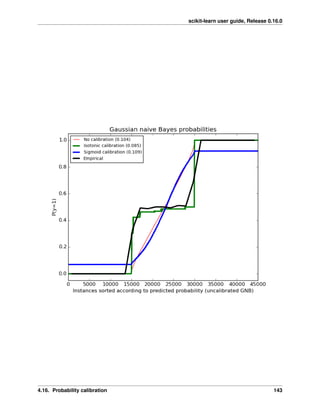


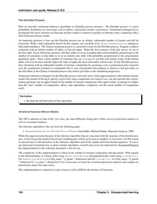
![scikit-learn user guide, Release 0.16.0
Update rules for VB inference
Here the full mathematical derivation of the Variational Bayes update rules for Gaussian Mixture Models is given. The
main parameters of the model, defined for any class 𝑘 ∈ [1..𝐾] are the class proportion 𝜑 𝑘, the mean parameters 𝜇 𝑘,
the covariance parameters Σ 𝑘, which is characterized by variational Wishart density, 𝑊 𝑖𝑠ℎ𝑎𝑟𝑡(𝑎 𝑘, Bk), where 𝑎 is
the degrees of freedom, and 𝐵 is the scale matrix. Depending on the covariance parametrization, 𝐵 𝑘 can be a positive
scalar, a positive vector or a Symmetric Positive Definite matrix.
The spherical model The model then is
𝜑 𝑘 ∼ 𝐵𝑒𝑡𝑎(1, 𝛼1)
𝜇 𝑘 ∼ 𝑁 𝑜𝑟𝑚𝑎𝑙(0, I)
𝜎 𝑘 ∼ 𝐺𝑎𝑚𝑚𝑎(1, 1)
𝑧𝑖 ∼ 𝑆𝐵𝑃(𝜑)
𝑋 𝑡 ∼ 𝑁 𝑜𝑟𝑚𝑎𝑙(𝜇 𝑧 𝑖
, 1
𝜎 𝑧 𝑖
I)
The variational distribution we’ll use is
𝜑 𝑘 ∼ 𝐵𝑒𝑡𝑎(𝛾 𝑘,1, 𝛾 𝑘,2)
𝜇 𝑘 ∼ 𝑁 𝑜𝑟𝑚𝑎𝑙(𝜈 𝜇 𝑘
, I)
𝜎 𝑘 ∼ 𝐺𝑎𝑚𝑚𝑎(𝑎 𝑘, 𝑏 𝑘)
𝑧𝑖 ∼ 𝐷𝑖𝑠𝑐𝑟𝑒𝑡𝑒(𝜈 𝑧 𝑖
)
The bound The variational bound is
log 𝑃(𝑋) ≥
∑︀
𝑘(𝐸 𝑞[log 𝑃(𝜑 𝑘)] − 𝐸 𝑞[log 𝑄(𝜑 𝑘)])
+
∑︀
𝑘 (𝐸 𝑞[log 𝑃(𝜇 𝑘)] − 𝐸 𝑞[log 𝑄(𝜇 𝑘)])
+
∑︀
𝑘 (𝐸 𝑞[log 𝑃(𝜎 𝑘)] − 𝐸 𝑞[log 𝑄(𝜎 𝑘)])
+
∑︀
𝑖 (𝐸 𝑞[log 𝑃(𝑧𝑖)] − 𝐸 𝑞[log 𝑄(𝑧𝑖)])
+
∑︀
𝑖 𝐸 𝑞[log 𝑃(𝑋 𝑡)]
The bound for 𝜑 𝑘
𝐸 𝑞[log 𝐵𝑒𝑡𝑎(1, 𝛼)] − 𝐸[log 𝐵𝑒𝑡𝑎(𝛾 𝑘,1, 𝛾 𝑘,2)] = log Γ(1 + 𝛼) − log Γ(𝛼)
+(𝛼 − 1)(Ψ(𝛾 𝑘,2) − Ψ(𝛾 𝑘,1 + 𝛾 𝑘,2))
− log Γ(𝛾 𝑘,1 + 𝛾 𝑘,2) + log Γ(𝛾 𝑘,1) + log Γ(𝛾 𝑘,2)
−(𝛾 𝑘,1 − 1)(Ψ(𝛾 𝑘,1) − Ψ(𝛾 𝑘,1 + 𝛾 𝑘,2))
−(𝛾 𝑘,2 − 1)(Ψ(𝛾 𝑘,2) − Ψ(𝛾 𝑘,1 + 𝛾 𝑘,2))
The bound for 𝜇 𝑘
𝐸 𝑞[log 𝑃(𝜇 𝑘)] − 𝐸 𝑞[log 𝑄(𝜇 𝑘)]
=
∫︀
𝑑𝜇 𝑓 𝑞(𝜇 𝑓 ) log 𝑃(𝜇 𝑓 ) −
∫︀
𝑑𝜇 𝑓 𝑞(𝜇 𝑓 ) log 𝑄(𝜇 𝑓 )
= − 𝐷
2 log 2𝜋 − 1
2 ||𝜈 𝜇 𝑘
||2
− 𝐷
2 + 𝐷
2 log 2𝜋𝑒
The bound for 𝜎 𝑘
Here I’ll use the inverse scale parametrization of the gamma distribution.
𝐸 𝑞[log 𝑃(𝜎 𝑘)] − 𝐸 𝑞[log 𝑄(𝜎 𝑘)]
= log Γ(𝑎 𝑘) − (𝑎 𝑘 − 1)Ψ(𝑎 𝑘) − log 𝑏 𝑘 + 𝑎 𝑘 − 𝑎 𝑘
𝑏 𝑘
The bound for z
𝐸 𝑞[log 𝑃(𝑧)] − 𝐸 𝑞[log 𝑄(𝑧)]
=
∑︀
𝑘
(︁(︁∑︀ 𝐾
𝑗=𝑘+1 𝜈 𝑧 𝑖,𝑗
)︁
(Ψ(𝛾 𝑘,2) − Ψ(𝛾 𝑘,1 + 𝛾 𝑘,2)) + 𝜈 𝑧 𝑖,𝑘
(Ψ(𝛾 𝑘,1) − Ψ(𝛾 𝑘,1 + 𝛾 𝑘,2)) − log 𝜈 𝑧 𝑖,𝑘
)︁
5.1. Gaussian mixture models 155](https://image.slidesharecdn.com/scikit-learn0-150409112902-conversion-gate01/85/Scikit-learn-0-16-0-user-guide-165-320.jpg)
![scikit-learn user guide, Release 0.16.0
The bound for 𝑋
Recall that there is no need for a 𝑄(𝑋) so this bound is just
𝐸 𝑞[log 𝑃(𝑋𝑖)] =
∑︀
𝑘 𝜈 𝑧 𝑘
(︁
− 𝐷
2 log 2𝜋 + 𝐷
2 (Ψ(𝑎 𝑘) − log(𝑏 𝑘)) − 𝑎 𝑘
2𝑏 𝑘
(||𝑋𝑖 − 𝜈 𝜇 𝑘
||2
+ 𝐷) − log 2𝜋𝑒
)︁
For simplicity I’ll later call the term inside the parenthesis 𝐸 𝑞[log 𝑃(𝑋𝑖|𝑧𝑖 = 𝑘)]
The updates Updating 𝛾
𝛾 𝑘,1 = 1 +
∑︀
𝑖 𝜈 𝑧 𝑖,𝑘
𝛾 𝑘,2 = 𝛼 +
∑︀
𝑖
∑︀
𝑗>𝑘 𝜈 𝑧 𝑖,𝑗
.
Updating 𝜇
The updates for mu essentially are just weighted expectations of 𝑋 regularized by the prior. We can see this by taking
the gradient of the bound with regards to 𝜈 𝜇 and setting it to zero. The gradient is
∇𝐿 = −𝜈 𝜇 𝑘
+
∑︁
𝑖
𝜈 𝑧 𝑖,𝑘
𝑏 𝑘
𝑎 𝑘
(𝑋𝑖 + −𝜈 𝜇)
so the update is
𝜈 𝜇 𝑘
=
∑︀
𝑖
𝜈 𝑧 𝑖,𝑘
𝑏 𝑘
𝑎 𝑘
𝑋𝑖
1 +
∑︀
𝑖
𝜈 𝑧 𝑖,𝑘
𝑏 𝑘
𝑎 𝑘
Updating 𝑎 and 𝑏
For some odd reason it doesn’t really work when you derive the updates for a and b using the gradients of the lower
bound (terms involving the Ψ′
function show up and 𝑎 is hard to isolate). However, we can use the other formula,
log 𝑄(𝜎 𝑘) = 𝐸 𝑣̸= 𝜎 𝑘
[log 𝑃] + 𝑐𝑜𝑛𝑠𝑡
All the terms not involving 𝜎 𝑘 get folded over into the constant and we get two terms: the prior and the probability of
𝑋. This gives us
log 𝑄(𝜎 𝑘) = −𝜎 𝑘 +
𝐷
2
∑︁
𝑖
𝜈 𝑧 𝑖,𝑘
log 𝜎 𝑘 −
𝜎 𝑘
2
∑︁
𝑖
𝜈 𝑧 𝑖,𝑘
(||𝑋𝑖 − 𝜇 𝑘||2
+ 𝐷)
This is the log of a gamma distribution, with 𝑎 𝑘 = 1 + 𝐷
2
∑︀
𝑖 𝜈 𝑧 𝑖,𝑘
and
𝑏 𝑘 = 1 +
1
2
∑︁
𝑖
𝜈 𝑧 𝑖,𝑘
(||𝑋𝑖 − 𝜇 𝑘||2
+ 𝐷).
You can verify this by normalizing the previous term.
Updating 𝑧
log 𝜈 𝑧 𝑖,𝑘
∝ Ψ(𝛾 𝑘,1) − Ψ(𝛾 𝑘,1 + 𝛾 𝑘,2) + 𝐸 𝑄[log 𝑃(𝑋𝑖|𝑧𝑖 = 𝑘)] +
∑︁
𝑗<𝑘
(Ψ(𝛾 𝑗,2) − Ψ(𝛾 𝑗,1 + 𝛾 𝑗,2)) .
The diagonal model The model then is
𝜑 𝑘 ∼ 𝐵𝑒𝑡𝑎(1, 𝛼1)
𝜇 𝑘 ∼ 𝑁 𝑜𝑟𝑚𝑎𝑙(0, I)
𝜎 𝑘,𝑑 ∼ 𝐺𝑎𝑚𝑚𝑎(1, 1)
𝑧𝑖 ∼ 𝑆𝐵𝑃(𝜑)
𝑋 𝑡 ∼ 𝑁 𝑜𝑟𝑚𝑎𝑙(𝜇 𝑧 𝑖
, 𝜎−1
𝑧 𝑖
)
156 Chapter 5. Unsupervised learning](https://image.slidesharecdn.com/scikit-learn0-150409112902-conversion-gate01/85/Scikit-learn-0-16-0-user-guide-166-320.jpg)
![scikit-learn user guide, Release 0.16.0
Tha variational distribution we’ll use is
𝜑 𝑘 ∼ 𝐵𝑒𝑡𝑎(𝛾 𝑘,1, 𝛾 𝑘,2)
𝜇 𝑘 ∼ 𝑁 𝑜𝑟𝑚𝑎𝑙(𝜈 𝜇 𝑘
, I)
𝜎 𝑘,𝑑 ∼ 𝐺𝑎𝑚𝑚𝑎(𝑎 𝑘,𝑑, 𝑏 𝑘,𝑑)
𝑧𝑖 ∼ 𝐷𝑖𝑠𝑐𝑟𝑒𝑡𝑒(𝜈 𝑧 𝑖
)
The lower bound The changes in this lower bound from the previous model are in the distributions of 𝜎 (as there
are a lot more 𝜎 s now) and 𝑋.
The bound for 𝜎 𝑘,𝑑 is the same bound for 𝜎 𝑘 and can be safely omitted.
The bound for 𝑋 :
The main difference here is that the precision matrix 𝜎 𝑘 scales the norm, so we have an extra term after computing the
expectation of 𝜇 𝑇
𝑘 𝜎 𝑘 𝜇 𝑘, which is 𝜈 𝑇
𝜇 𝑘
𝜎 𝑘 𝜈 𝜇 𝑘
+
∑︀
𝑑 𝜎 𝑘,𝑑. We then have
𝐸 𝑞[log 𝑃(𝑋𝑖)] =
∑︀
𝑘 𝜈 𝑧 𝑘
(︁
− 𝐷
2 log 2𝜋 + 1
2
∑︀
𝑑(Ψ(𝑎 𝑘,𝑑) − log(𝑏 𝑘,𝑑))
−1
2 ((𝑋𝑖 − 𝜈 𝜇 𝑘
) 𝑇 𝑎 𝑘
𝑏 𝑘
(𝑋𝑖 − 𝜈 𝜇 𝑘
) +
∑︀
𝑑 𝜎 𝑘,𝑑) − log 2𝜋𝑒
)︁
The updates The updates only chance for 𝜇 (to weight them with the new 𝜎), 𝑧 (but the change is all folded into the
𝐸 𝑞[𝑃(𝑋𝑖|𝑧𝑖 = 𝑘)] term), and the 𝑎 and 𝑏 variables themselves.
The update for 𝜇
𝜈 𝜇 𝑘
=
(︃
I +
∑︁
𝑖
𝜈 𝑧 𝑖,𝑘
bk
ak
)︃−1 (︃
∑︁
𝑖
𝜈 𝑧 𝑖,𝑘
𝑏 𝑘
𝑎 𝑘
𝑋𝑖
)︃
The updates for a and b
Here we’ll do something very similar to the spheric model. The main difference is that now each 𝜎 𝑘,𝑑 controls only
one dimension of the bound:
log 𝑄(𝜎 𝑘,𝑑) = −𝜎 𝑘,𝑑 +
∑︁
𝑖
𝜈 𝑧 𝑖,𝑘
1
2
log 𝜎 𝑘,𝑑 −
𝜎 𝑘,𝑑
2
∑︁
𝑖
𝜈 𝑧 𝑖,𝑘
((𝑋𝑖,𝑑 − 𝜇 𝑘,𝑑)2
+ 1)
Hence
𝑎 𝑘,𝑑 = 1 +
1
2
∑︁
𝑖
𝜈 𝑧 𝑖,𝑘
𝑏 𝑘,𝑑 = 1 +
1
2
∑︁
𝑖
𝜈 𝑧 𝑖,𝑘
((𝑋𝑖,𝑑 − 𝜇 𝑘,𝑑)2
+ 1)
The tied model The model then is
𝜑 𝑘 ∼ 𝐵𝑒𝑡𝑎(1, 𝛼1)
𝜇 𝑘 ∼ 𝑁 𝑜𝑟𝑚𝑎𝑙(0, I)
Σ ∼ 𝑊 𝑖𝑠ℎ𝑎𝑟𝑡(𝐷, I)
𝑧𝑖 ∼ 𝑆𝐵𝑃(𝜑)
𝑋 𝑡 ∼ 𝑁 𝑜𝑟𝑚𝑎𝑙(𝜇 𝑧 𝑖
, Σ−1
)
Tha variational distribution we’ll use is
𝜑 𝑘 ∼ 𝐵𝑒𝑡𝑎(𝛾 𝑘,1, 𝛾 𝑘,2)
𝜇 𝑘 ∼ 𝑁 𝑜𝑟𝑚𝑎𝑙(𝜈 𝜇 𝑘
, I)
Σ ∼ 𝑊 𝑖𝑠ℎ𝑎𝑟𝑡(𝑎, B)
𝑧𝑖 ∼ 𝐷𝑖𝑠𝑐𝑟𝑒𝑡𝑒(𝜈 𝑧 𝑖
)
5.1. Gaussian mixture models 157](https://image.slidesharecdn.com/scikit-learn0-150409112902-conversion-gate01/85/Scikit-learn-0-16-0-user-guide-167-320.jpg)
![scikit-learn user guide, Release 0.16.0
The lower bound There are two changes in the lower-bound: for Σ and for 𝑋.
The bound for Σ
𝐷2
2 log 2 +
∑︀
𝑑 log Γ( 𝐷+1−𝑑
2 )
− 𝑎𝐷
2 log 2 + 𝑎
2 log |B| +
∑︀
𝑑 log Γ( 𝑎+1−𝑑
2 )
+ 𝑎−𝐷
2
(︀∑︀
𝑑 Ψ
(︀ 𝑎+1−𝑑
2
)︀
+ 𝐷 log 2 + log |B|
)︀
+1
2 𝑎tr[B − I]
The bound for X
𝐸 𝑞[log 𝑃(𝑋𝑖)] =
∑︀
𝑘 𝜈 𝑧 𝑘
(︁
− 𝐷
2 log 2𝜋 + 1
2
(︀∑︀
𝑑 Ψ
(︀ 𝑎+1−𝑑
2
)︀
+ 𝐷 log 2 + log |B|
)︀
−1
2 ((𝑋𝑖 − 𝜈 𝜇 𝑘
)𝑎B(𝑋𝑖 − 𝜈 𝜇 𝑘
) + 𝑎tr(B)) − log 2𝜋𝑒
)︁
The updates As in the last setting, what changes are the trivial update for 𝑧, the update for 𝜇 and the update for 𝑎
and B.
The update for 𝜇
𝜈 𝜇 𝑘
=
(︃
I + 𝑎B
∑︁
𝑖
𝜈 𝑧 𝑖,𝑘
)︃−1 (︃
𝑎B
∑︁
𝑖
𝜈 𝑧 𝑖,𝑘
𝑋𝑖
)︃
The update for 𝑎 and 𝐵
As this distribution is far too complicated I’m not even going to try going at it the gradient way.
log 𝑄(Σ) = +
1
2
log |Σ| −
1
2
tr[Σ] +
∑︁
𝑖
∑︁
𝑘
𝜈 𝑧 𝑖,𝑘
(︂
+
1
2
log |Σ| −
1
2
((𝑋𝑖 − 𝜈 𝜇 𝑘
) 𝑇
Σ(𝑋𝑖 − 𝜈 𝜇 𝑘
) + tr[Σ])
)︂
which non-trivially (seeing that the quadratic form with Σ in the middle can be expressed as the trace of something)
reduces to
log 𝑄(Σ) = +
1
2
log |Σ| −
1
2
tr[Σ] +
∑︁
𝑖
∑︁
𝑘
𝜈 𝑧 𝑖,𝑘
(︂
+
1
2
log |Σ| −
1
2
(tr[(𝑋𝑖 − 𝜈 𝜇 𝑘
)(𝑋𝑖 − 𝜈 𝜇 𝑘
) 𝑇
Σ] + tr[𝐼Σ])
)︂
hence this (with a bit of squinting) looks like a wishart with parameters
𝑎 = 2 + 𝐷 + 𝑇
and
B =
(︃
I +
∑︁
𝑖
∑︁
𝑘
𝜈 𝑧 𝑖,𝑘
(𝑋𝑖 − 𝜈 𝜇 𝑘
)(𝑋𝑖 − 𝜈 𝜇 𝑘
) 𝑇
)︃−1
The full model
The model then is
𝜑 𝑘 ∼ 𝐵𝑒𝑡𝑎(1, 𝛼1)
𝜇 𝑘 ∼ 𝑁 𝑜𝑟𝑚𝑎𝑙(0, I)
Σ 𝑘 ∼ 𝑊 𝑖𝑠ℎ𝑎𝑟𝑡(𝐷, I)
𝑧𝑖 ∼ 𝑆𝐵𝑃(𝜑)
𝑋 𝑡 ∼ 𝑁 𝑜𝑟𝑚𝑎𝑙(𝜇 𝑧 𝑖
, Σ−1
𝑧,𝑖 )
The variational distribution we’ll use is
𝜑 𝑘 ∼ 𝐵𝑒𝑡𝑎(𝛾 𝑘,1, 𝛾 𝑘,2)
𝜇 𝑘 ∼ 𝑁 𝑜𝑟𝑚𝑎𝑙(𝜈 𝜇 𝑘
, I)
Σ 𝑘 ∼ 𝑊 𝑖𝑠ℎ𝑎𝑟𝑡(𝑎 𝑘, Bk)
𝑧𝑖 ∼ 𝐷𝑖𝑠𝑐𝑟𝑒𝑡𝑒(𝜈 𝑧 𝑖
)
158 Chapter 5. Unsupervised learning](https://image.slidesharecdn.com/scikit-learn0-150409112902-conversion-gate01/85/Scikit-learn-0-16-0-user-guide-168-320.jpg)
![scikit-learn user guide, Release 0.16.0
The lower bound All that changes in this lower bound in comparison to the previous one is that there are K priors
on different Σ precision matrices and there are the correct indices on the bound for X.
The updates All that changes in the updates is that the update for mu uses only the proper sigma and the updates
for a and B don’t have a sum over K, so
𝜈 𝜇 𝑘
=
(︃
I + 𝑎 𝑘Bk
∑︁
𝑖
𝜈 𝑧 𝑖,𝑘
)︃−1 (︃
𝑎 𝑘Bk
∑︁
𝑖
𝜈 𝑧 𝑖,𝑘
𝑋𝑖
)︃
𝑎 𝑘 = 2 + 𝐷 +
∑︁
𝑖
𝜈 𝑧 𝑖,𝑘
and
B =
(︃(︃
∑︁
𝑖
𝜈 𝑧 𝑖,𝑘
+ 1
)︃
I +
∑︁
𝑖
𝜈 𝑧 𝑖,𝑘
(𝑋𝑖 − 𝜈 𝜇 𝑘
)(𝑋𝑖 − 𝜈 𝜇 𝑘
) 𝑇
)︃−1
5.2 Manifold learning
Look for the bare necessities
The simple bare necessities
Forget about your worries and your strife
I mean the bare necessities
Old Mother Nature’s recipes
That bring the bare necessities of life
– Baloo’s song [The Jungle Book]
Manifold learning is an approach to non-linear dimensionality reduction. Algorithms for this task are based on the
idea that the dimensionality of many data sets is only artificially high.
5.2.1 Introduction
High-dimensional datasets can be very difficult to visualize. While data in two or three dimensions can be plotted to
show the inherent structure of the data, equivalent high-dimensional plots are much less intuitive. To aid visualization
of the structure of a dataset, the dimension must be reduced in some way.
5.2. Manifold learning 159](https://image.slidesharecdn.com/scikit-learn0-150409112902-conversion-gate01/85/Scikit-learn-0-16-0-user-guide-169-320.jpg)
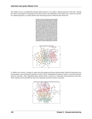

![scikit-learn user guide, Release 0.16.0
Complexity
The Isomap algorithm comprises three stages:
1. Nearest neighbor search. Isomap uses sklearn.neighbors.BallTree for efficient neighbor search.
The cost is approximately 𝑂[𝐷 log(𝑘)𝑁 log(𝑁)], for 𝑘 nearest neighbors of 𝑁 points in 𝐷 dimensions.
2. Shortest-path graph search. The most efficient known algorithms for this are Dijkstra’s Algorithm, which is
approximately 𝑂[𝑁2
(𝑘 + log(𝑁))], or the Floyd-Warshall algorithm, which is 𝑂[𝑁3
]. The algorithm can be
selected by the user with the path_method keyword of Isomap. If unspecified, the code attempts to choose
the best algorithm for the input data.
3. Partial eigenvalue decomposition. The embedding is encoded in the eigenvectors corresponding to the 𝑑
largest eigenvalues of the 𝑁 × 𝑁 isomap kernel. For a dense solver, the cost is approximately 𝑂[𝑑𝑁2
]. This
cost can often be improved using the ARPACK solver. The eigensolver can be specified by the user with the
path_method keyword of Isomap. If unspecified, the code attempts to choose the best algorithm for the
input data.
The overall complexity of Isomap is 𝑂[𝐷 log(𝑘)𝑁 log(𝑁)] + 𝑂[𝑁2
(𝑘 + log(𝑁))] + 𝑂[𝑑𝑁2
].
• 𝑁 : number of training data points
• 𝐷 : input dimension
• 𝑘 : number of nearest neighbors
• 𝑑 : output dimension
References:
• “A global geometric framework for nonlinear dimensionality reduction” Tenenbaum, J.B.; De Silva, V.; &
Langford, J.C. Science 290 (5500)
5.2.3 Locally Linear Embedding
Locally linear embedding (LLE) seeks a lower-dimensional projection of the data which preserves distances within
local neighborhoods. It can be thought of as a series of local Principal Component Analyses which are globally
compared to find the best non-linear embedding.
Locally linear embedding can be performed with function locally_linear_embedding or its object-oriented
counterpart LocallyLinearEmbedding.
162 Chapter 5. Unsupervised learning](https://image.slidesharecdn.com/scikit-learn0-150409112902-conversion-gate01/85/Scikit-learn-0-16-0-user-guide-172-320.jpg)
![scikit-learn user guide, Release 0.16.0
Complexity
The standard LLE algorithm comprises three stages:
1. Nearest Neighbors Search. See discussion under Isomap above.
2. Weight Matrix Construction. 𝑂[𝐷𝑁 𝑘3
]. The construction of the LLE weight matrix involves the solution of
a 𝑘 × 𝑘 linear equation for each of the 𝑁 local neighborhoods
3. Partial Eigenvalue Decomposition. See discussion under Isomap above.
The overall complexity of standard LLE is 𝑂[𝐷 log(𝑘)𝑁 log(𝑁)] + 𝑂[𝐷𝑁 𝑘3
] + 𝑂[𝑑𝑁2
].
• 𝑁 : number of training data points
• 𝐷 : input dimension
• 𝑘 : number of nearest neighbors
• 𝑑 : output dimension
References:
• “Nonlinear dimensionality reduction by locally linear embedding” Roweis, S. & Saul, L. Science
290:2323 (2000)
5.2.4 Modified Locally Linear Embedding
One well-known issue with LLE is the regularization problem. When the number of neighbors is greater than the
number of input dimensions, the matrix defining each local neighborhood is rank-deficient. To address this, standard
LLE applies an arbitrary regularization parameter 𝑟, which is chosen relative to the trace of the local weight matrix.
Though it can be shown formally that as 𝑟 → 0, the solution converges to the desired embedding, there is no guarantee
that the optimal solution will be found for 𝑟 > 0. This problem manifests itself in embeddings which distort the
underlying geometry of the manifold.
One method to address the regularization problem is to use multiple weight vectors in each neighborhood.
This is the essence of modified locally linear embedding (MLLE). MLLE can be performed with function
locally_linear_embedding or its object-oriented counterpart LocallyLinearEmbedding, with the key-
word method = ’modified’. It requires n_neighbors > n_components.
5.2. Manifold learning 163](https://image.slidesharecdn.com/scikit-learn0-150409112902-conversion-gate01/85/Scikit-learn-0-16-0-user-guide-173-320.jpg)
![scikit-learn user guide, Release 0.16.0
Complexity
The MLLE algorithm comprises three stages:
1. Nearest Neighbors Search. Same as standard LLE
2. Weight Matrix Construction. Approximately 𝑂[𝐷𝑁 𝑘3
]+𝑂[𝑁(𝑘−𝐷)𝑘2
]. The first term is exactly equivalent
to that of standard LLE. The second term has to do with constructing the weight matrix from multiple weights.
In practice, the added cost of constructing the MLLE weight matrix is relatively small compared to the cost of
steps 1 and 3.
3. Partial Eigenvalue Decomposition. Same as standard LLE
The overall complexity of MLLE is 𝑂[𝐷 log(𝑘)𝑁 log(𝑁)] + 𝑂[𝐷𝑁 𝑘3
] + 𝑂[𝑁(𝑘 − 𝐷)𝑘2
] + 𝑂[𝑑𝑁2
].
• 𝑁 : number of training data points
• 𝐷 : input dimension
• 𝑘 : number of nearest neighbors
• 𝑑 : output dimension
References:
• “MLLE: Modified Locally Linear Embedding Using Multiple Weights” Zhang, Z. & Wang, J.
5.2.5 Hessian Eigenmapping
Hessian Eigenmapping (also known as Hessian-based LLE: HLLE) is another method of solving the regularization
problem of LLE. It revolves around a hessian-based quadratic form at each neighborhood which is used to recover
the locally linear structure. Though other implementations note its poor scaling with data size, sklearn imple-
ments some algorithmic improvements which make its cost comparable to that of other LLE variants for small output
dimension. HLLE can be performed with function locally_linear_embedding or its object-oriented counter-
part LocallyLinearEmbedding, with the keyword method = ’hessian’. It requires n_neighbors >
n_components * (n_components + 3) / 2.
164 Chapter 5. Unsupervised learning](https://image.slidesharecdn.com/scikit-learn0-150409112902-conversion-gate01/85/Scikit-learn-0-16-0-user-guide-174-320.jpg)
![scikit-learn user guide, Release 0.16.0
Complexity
The HLLE algorithm comprises three stages:
1. Nearest Neighbors Search. Same as standard LLE
2. Weight Matrix Construction. Approximately 𝑂[𝐷𝑁 𝑘3
] + 𝑂[𝑁 𝑑6
]. The first term reflects a similar cost to
that of standard LLE. The second term comes from a QR decomposition of the local hessian estimator.
3. Partial Eigenvalue Decomposition. Same as standard LLE
The overall complexity of standard HLLE is 𝑂[𝐷 log(𝑘)𝑁 log(𝑁)] + 𝑂[𝐷𝑁 𝑘3
] + 𝑂[𝑁 𝑑6
] + 𝑂[𝑑𝑁2
].
• 𝑁 : number of training data points
• 𝐷 : input dimension
• 𝑘 : number of nearest neighbors
• 𝑑 : output dimension
References:
• “Hessian Eigenmaps: Locally linear embedding techniques for high-dimensional data” Donoho, D. &
Grimes, C. Proc Natl Acad Sci USA. 100:5591 (2003)
5.2.6 Spectral Embedding
Spectral Embedding (also known as Laplacian Eigenmaps) is one method to calculate non-linear embedding. It finds
a low dimensional representation of the data using a spectral decomposition of the graph Laplacian. The graph gen-
erated can be considered as a discrete approximation of the low dimensional manifold in the high dimensional space.
Minimization of a cost function based on the graph ensures that points close to each other on the manifold are mapped
close to each other in the low dimensional space, preserving local distances. Spectral embedding can be performed
with the function spectral_embedding or its object-oriented counterpart SpectralEmbedding.
Complexity
The Spectral Embedding algorithm comprises three stages:
1. Weighted Graph Construction. Transform the raw input data into graph representation using affinity (adja-
cency) matrix representation.
2. Graph Laplacian Construction. unnormalized Graph Laplacian is constructed as 𝐿 = 𝐷 − 𝐴 for and normal-
ized one as 𝐿 = 𝐷− 1
2 (𝐷 − 𝐴)𝐷− 1
2 .
3. Partial Eigenvalue Decomposition. Eigenvalue decomposition is done on graph Laplacian
The overall complexity of spectral embedding is 𝑂[𝐷 log(𝑘)𝑁 log(𝑁)] + 𝑂[𝐷𝑁 𝑘3
] + 𝑂[𝑑𝑁2
].
• 𝑁 : number of training data points
• 𝐷 : input dimension
• 𝑘 : number of nearest neighbors
• 𝑑 : output dimension
5.2. Manifold learning 165](https://image.slidesharecdn.com/scikit-learn0-150409112902-conversion-gate01/85/Scikit-learn-0-16-0-user-guide-175-320.jpg)
![scikit-learn user guide, Release 0.16.0
References:
• “Laplacian Eigenmaps for Dimensionality Reduction and Data Representation” M. Belkin, P. Niyogi,
Neural Computation, June 2003; 15 (6):1373-1396
5.2.7 Local Tangent Space Alignment
Though not technically a variant of LLE, Local tangent space alignment (LTSA) is algorithmically similar enough
to LLE that it can be put in this category. Rather than focusing on preserving neighborhood distances as in LLE,
LTSA seeks to characterize the local geometry at each neighborhood via its tangent space, and performs a global
optimization to align these local tangent spaces to learn the embedding. LTSA can be performed with function
locally_linear_embedding or its object-oriented counterpart LocallyLinearEmbedding, with the key-
word method = ’ltsa’.
Complexity
The LTSA algorithm comprises three stages:
1. Nearest Neighbors Search. Same as standard LLE
2. Weight Matrix Construction. Approximately 𝑂[𝐷𝑁 𝑘3
] + 𝑂[𝑘2
𝑑]. The first term reflects a similar cost to that
of standard LLE.
3. Partial Eigenvalue Decomposition. Same as standard LLE
The overall complexity of standard LTSA is 𝑂[𝐷 log(𝑘)𝑁 log(𝑁)] + 𝑂[𝐷𝑁 𝑘3
] + 𝑂[𝑘2
𝑑] + 𝑂[𝑑𝑁2
].
• 𝑁 : number of training data points
• 𝐷 : input dimension
• 𝑘 : number of nearest neighbors
• 𝑑 : output dimension
166 Chapter 5. Unsupervised learning](https://image.slidesharecdn.com/scikit-learn0-150409112902-conversion-gate01/85/Scikit-learn-0-16-0-user-guide-176-320.jpg)


![scikit-learn user guide, Release 0.16.0
gaps between natural clusters in the data. If the factor is too high, the KL divergence could increase during this phase.
Usually it does not have to be tuned. A critical parameter is the learning rate. If it is too low gradient descent will get
stuck in a bad local minimum. If it is too high the KL divergence will increase during optimization. More tips can be
found in Laurens van der Maaten’s FAQ (see references).
Standard t-SNE that has been implemented here is usually much slower than other manifold learning algorithms. The
optimization is quite difficult and the computation of the gradient is on 𝑂[𝑑𝑁2
], where 𝑑 is the number of output
dimensions and 𝑁 is the number of samples.
While Isomap, LLE and variants are best suited to unfold a single continuous low dimensional manifold, t-SNE will
focus on the local structure of the data and will tend to extract clustered local groups of samples as highlighted on the
S-curve example. This ability to group samples based on the local structure might be beneficial to visually disentangle
a dataset that comprises several manifolds at once as is the case in the digits dataset.
Also note that the digits labels roughly match the natural grouping found by t-SNE while the linear 2D projection of
the PCA model yields a representation where label regions largely overlap. This is a strong clue that this data can be
well separated by non linear methods that focus on the local structure (e.g. an SVM with a Gaussian RBF kernel).
However, failing to visualize well separated homogeneously labeled groups with t-SNE in 2D does not necessarily
implie that the data cannot be correctly classified by a supervised model. It might be the case that 2 dimensions are
not enough low to accurately represents the internal structure of the data.
References:
• “Visualizing High-Dimensional Data Using t-SNE” van der Maaten, L.J.P.; Hinton, G. Journal of Machine
Learning Research (2008)
• “t-Distributed Stochastic Neighbor Embedding” van der Maaten, L.J.P.
5.2.10 Tips on practical use
• Make sure the same scale is used over all features. Because manifold learning methods are based on a nearest-
neighbor search, the algorithm may perform poorly otherwise. See StandardScaler for convenient ways of
scaling heterogeneous data.
• The reconstruction error computed by each routine can be used to choose the optimal output dimension. For a
𝑑-dimensional manifold embedded in a 𝐷-dimensional parameter space, the reconstruction error will decrease
as n_components is increased until n_components == d.
• Note that noisy data can “short-circuit” the manifold, in essence acting as a bridge between parts of the manifold
5.2. Manifold learning 169](https://image.slidesharecdn.com/scikit-learn0-150409112902-conversion-gate01/85/Scikit-learn-0-16-0-user-guide-179-320.jpg)
![scikit-learn user guide, Release 0.16.0
that would otherwise be well-separated. Manifold learning on noisy and/or incomplete data is an active area of
research.
• Certain input configurations can lead to singular weight matrices, for example when more than two points in the
dataset are identical, or when the data is split into disjointed groups. In this case, solver=’arpack’ will
fail to find the null space. The easiest way to address this is to use solver=’dense’ which will work on a
singular matrix, though it may be very slow depending on the number of input points. Alternatively, one can
attempt to understand the source of the singularity: if it is due to disjoint sets, increasing n_neighbors may
help. If it is due to identical points in the dataset, removing these points may help.
See also:
Totally Random Trees Embedding can also be useful to derive non-linear representations of feature space, also it does
not perform dimensionality reduction.
5.3 Clustering
Clustering of unlabeled data can be performed with the module sklearn.cluster.
Each clustering algorithm comes in two variants: a class, that implements the fit method to learn the clusters on train
data, and a function, that, given train data, returns an array of integer labels corresponding to the different clusters. For
the class, the labels over the training data can be found in the labels_ attribute.
Input data
One important thing to note is that the algorithms implemented in this module take different kinds of ma-
trix as input. On one hand, MeanShift and KMeans take data matrices of shape [n_samples, n_features].
These can be obtained from the classes in the sklearn.feature_extraction module. On the
other hand, AffinityPropagation and SpectralClustering take similarity matrices of shape
[n_samples, n_samples]. These can be obtained from the functions in the sklearn.metrics.pairwise
module. In other words, MeanShift and KMeans work with points in a vector space, whereas
AffinityPropagation and SpectralClustering can work with arbitrary objects, as long as a simi-
larity measure exists for such objects.
5.3.1 Overview of clustering methods
Fig. 5.2: A comparison of the clustering algorithms in scikit-learn
170 Chapter 5. Unsupervised learning](https://image.slidesharecdn.com/scikit-learn0-150409112902-conversion-gate01/85/Scikit-learn-0-16-0-user-guide-180-320.jpg)
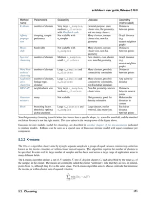

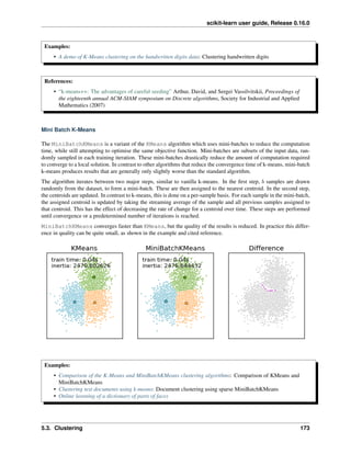

![scikit-learn user guide, Release 0.16.0
More formally, the responsibility of a sample 𝑘 to be the exemplar of sample 𝑖 is given by:
𝑟(𝑖, 𝑘) ← 𝑠(𝑖, 𝑘) − 𝑚𝑎𝑥[𝑎(𝑖, ´𝑘) + 𝑠(𝑖, ´𝑘)∀´𝑘 ̸= 𝑘]
Where 𝑠(𝑖, 𝑘) is the similarity between samples 𝑖 and 𝑘. The availability of sample 𝑘 to be the exemplar of sample 𝑖 is
given by:
𝑎(𝑖, 𝑘) ← 𝑚𝑖𝑛[0, 𝑟(𝑘, 𝑘) +
∑︁
´𝑖 𝑠.𝑡. ´𝑖/∈{𝑖,𝑘}
𝑟(´𝑖, 𝑘)]
To begin with, all values for 𝑟 and 𝑎 are set to zero, and the calculation of each iterates until convergence.
5.3.4 Mean Shift
MeanShift clustering aims to discover blobs in a smooth density of samples. It is a centroid based algorithm, which
works by updating candidates for centroids to be the mean of the points within a given region. These candidates are
then filtered in a post-processing stage to eliminate near-duplicates to form the final set of centroids.
Given a candidate centroid 𝑥𝑖 for iteration 𝑡, the candidate is updated according to the following equation:
𝑥 𝑡+1
𝑖 = 𝑥 𝑡
𝑖 + 𝑚(𝑥 𝑡
𝑖)
Where 𝑁(𝑥𝑖) is the neighborhood of samples within a given distance around 𝑥𝑖 and 𝑚 is the mean shift vector that
is computed for each centroid that points towards a region of the maximum increase in the density of points. This
is computed using the following equation, effectively updating a centroid to be the mean of the samples within its
neighborhood:
𝑚(𝑥𝑖) =
∑︀
𝑥 𝑗 ∈𝑁(𝑥 𝑖) 𝐾(𝑥 𝑗 − 𝑥𝑖)𝑥 𝑗
∑︀
𝑥 𝑗 ∈𝑁(𝑥 𝑖) 𝐾(𝑥 𝑗 − 𝑥𝑖)
The algorithm automatically sets the number of clusters, instead of relying on a parameter bandwidth, which dictates
the size of the region to search through. This parameter can be set manually, but can be estimated using the provided
estimate_bandwidth function, which is called if the bandwidth is not set.
The algorithm is not highly scalable, as it requires multiple nearest neighbor searches during the execution of the
algorithm. The algorithm is guaranteed to converge, however the algorithm will stop iterating when the change in
centroids is small.
Labelling a new sample is performed by finding the nearest centroid for a given sample.
5.3. Clustering 175](https://image.slidesharecdn.com/scikit-learn0-150409112902-conversion-gate01/85/Scikit-learn-0-16-0-user-guide-185-320.jpg)
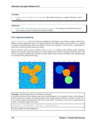


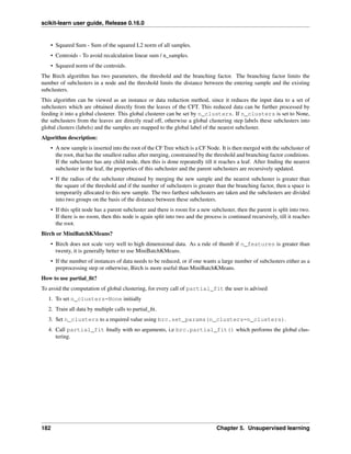
![scikit-learn user guide, Release 0.16.0
References:
• Tian Zhang, Raghu Ramakrishnan, Maron Livny BIRCH: An efficient data clustering method for large
databases. http://www.cs.sfu.ca/CourseCentral/459/han/papers/zhang96.pdf
• Roberto Perdisci JBirch - Java implementation of BIRCH clustering algorithm
https://code.google.com/p/jbirch/
5.3.9 Clustering performance evaluation
Evaluating the performance of a clustering algorithm is not as trivial as counting the number of errors or the precision
and recall of a supervised classification algorithm. In particular any evaluation metric should not take the absolute
values of the cluster labels into account but rather if this clustering define separations of the data similar to some
ground truth set of classes or satisfying some assumption such that members belong to the same class are more similar
that members of different classes according to some similarity metric.
Adjusted Rand index
Presentation and usage
Given the knowledge of the ground truth class assignments labels_true and our clustering algorithm assignments
of the same samples labels_pred, the adjusted Rand index is a function that measures the similarity of the two
assignments, ignoring permutations and with chance normalization:
>>> from sklearn import metrics
>>> labels_true = [0, 0, 0, 1, 1, 1]
>>> labels_pred = [0, 0, 1, 1, 2, 2]
>>> metrics.adjusted_rand_score(labels_true, labels_pred)
0.24...
One can permute 0 and 1 in the predicted labels, rename 2 to 3, and get the same score:
>>> labels_pred = [1, 1, 0, 0, 3, 3]
>>> metrics.adjusted_rand_score(labels_true, labels_pred)
0.24...
Furthermore, adjusted_rand_score is symmetric: swapping the argument does not change the score. It can
thus be used as a consensus measure:
5.3. Clustering 183](https://image.slidesharecdn.com/scikit-learn0-150409112902-conversion-gate01/85/Scikit-learn-0-16-0-user-guide-193-320.jpg)
![scikit-learn user guide, Release 0.16.0
>>> metrics.adjusted_rand_score(labels_pred, labels_true)
0.24...
Perfect labeling is scored 1.0:
>>> labels_pred = labels_true[:]
>>> metrics.adjusted_rand_score(labels_true, labels_pred)
1.0
Bad (e.g. independent labelings) have negative or close to 0.0 scores:
>>> labels_true = [0, 1, 2, 0, 3, 4, 5, 1]
>>> labels_pred = [1, 1, 0, 0, 2, 2, 2, 2]
>>> metrics.adjusted_rand_score(labels_true, labels_pred)
-0.12...
Advantages
• Random (uniform) label assignments have a ARI score close to 0.0 for any value of n_clusters and
n_samples (which is not the case for raw Rand index or the V-measure for instance).
• Bounded range [-1, 1]: negative values are bad (independent labelings), similar clusterings have a positive ARI,
1.0 is the perfect match score.
• No assumption is made on the cluster structure: can be used to compare clustering algorithms such as k-
means which assumes isotropic blob shapes with results of spectral clustering algorithms which can find cluster
with “folded” shapes.
Drawbacks
• Contrary to inertia, ARI requires knowledge of the ground truth classes while is almost never available in
practice or requires manual assignment by human annotators (as in the supervised learning setting).
However ARI can also be useful in a purely unsupervised setting as a building block for a Consensus Index that
can be used for clustering model selection (TODO).
Examples:
• Adjustment for chance in clustering performance evaluation: Analysis of the impact of the dataset size on
the value of clustering measures for random assignments.
Mathematical formulation
If C is a ground truth class assignment and K the clustering, let us define 𝑎 and 𝑏 as:
• 𝑎, the number of pairs of elements that are in the same set in C and in the same set in K
• 𝑏, the number of pairs of elements that are in different sets in C and in different sets in K
The raw (unadjusted) Rand index is then given by:
RI =
𝑎 + 𝑏
𝐶
𝑛 𝑠𝑎𝑚𝑝𝑙𝑒𝑠
2
Where 𝐶
𝑛 𝑠𝑎𝑚𝑝𝑙𝑒𝑠
2 is the total number of possible pairs in the dataset (without ordering).
184 Chapter 5. Unsupervised learning](https://image.slidesharecdn.com/scikit-learn0-150409112902-conversion-gate01/85/Scikit-learn-0-16-0-user-guide-194-320.jpg)
![scikit-learn user guide, Release 0.16.0
However the RI score does not guarantee that random label assignments will get a value close to zero (esp. if the
number of clusters is in the same order of magnitude as the number of samples).
To counter this effect we can discount the expected RI 𝐸[RI] of random labelings by defining the adjusted Rand index
as follows:
ARI =
RI − 𝐸[RI]
max(RI) − 𝐸[RI]
References
• Comparing Partitions L. Hubert and P. Arabie, Journal of Classification 1985
• Wikipedia entry for the adjusted Rand index
Mutual Information based scores
Presentation and usage
Given the knowledge of the ground truth class assignments labels_true and our clustering algorithm assignments
of the same samples labels_pred, the Mutual Information is a function that measures the agreement of the two
assignments, ignoring permutations. Two different normalized versions of this measure are available, Normalized
Mutual Information(NMI) and Adjusted Mutual Information(AMI). NMI is often used in the literature while
AMI was proposed more recently and is normalized against chance:
>>> from sklearn import metrics
>>> labels_true = [0, 0, 0, 1, 1, 1]
>>> labels_pred = [0, 0, 1, 1, 2, 2]
>>> metrics.adjusted_mutual_info_score(labels_true, labels_pred)
0.22504...
One can permute 0 and 1 in the predicted labels, rename 2 to 3 and get the same score:
>>> labels_pred = [1, 1, 0, 0, 3, 3]
>>> metrics.adjusted_mutual_info_score(labels_true, labels_pred)
0.22504...
All, mutual_info_score, adjusted_mutual_info_score and normalized_mutual_info_score
are symmetric: swapping the argument does not change the score. Thus they can be used as a consensus measure:
>>> metrics.adjusted_mutual_info_score(labels_pred, labels_true)
0.22504...
Perfect labeling is scored 1.0:
>>> labels_pred = labels_true[:]
>>> metrics.adjusted_mutual_info_score(labels_true, labels_pred)
1.0
>>> metrics.normalized_mutual_info_score(labels_true, labels_pred)
1.0
This is not true for mutual_info_score, which is therefore harder to judge:
>>> metrics.mutual_info_score(labels_true, labels_pred)
0.69...
Bad (e.g. independent labelings) have non-positive scores:
5.3. Clustering 185](https://image.slidesharecdn.com/scikit-learn0-150409112902-conversion-gate01/85/Scikit-learn-0-16-0-user-guide-195-320.jpg)
![scikit-learn user guide, Release 0.16.0
>>> labels_true = [0, 1, 2, 0, 3, 4, 5, 1]
>>> labels_pred = [1, 1, 0, 0, 2, 2, 2, 2]
>>> metrics.adjusted_mutual_info_score(labels_true, labels_pred)
-0.10526...
Advantages
• Random (uniform) label assignments have a AMI score close to 0.0 for any value of n_clusters and
n_samples (which is not the case for raw Mutual Information or the V-measure for instance).
• Bounded range [0, 1]: Values close to zero indicate two label assignments that are largely independent, while
values close to one indicate significant agreement. Further, values of exactly 0 indicate purely independent
label assignments and a AMI of exactly 1 indicates that the two label assignments are equal (with or without
permutation).
• No assumption is made on the cluster structure: can be used to compare clustering algorithms such as k-
means which assumes isotropic blob shapes with results of spectral clustering algorithms which can find cluster
with “folded” shapes.
Drawbacks
• Contrary to inertia, MI-based measures require the knowledge of the ground truth classes while almost
never available in practice or requires manual assignment by human annotators (as in the supervised learning
setting).
However MI-based measures can also be useful in purely unsupervised setting as a building block for a Consen-
sus Index that can be used for clustering model selection.
• NMI and MI are not adjusted against chance.
Examples:
• Adjustment for chance in clustering performance evaluation: Analysis of the impact of the dataset size on
the value of clustering measures for random assignments. This example also includes the Adjusted Rand
Index.
Mathematical formulation
Assume two label assignments (of the same N objects), 𝑈 and 𝑉 . Their entropy is the amount of uncertainty for a
partition set, defined by:
𝐻(𝑈) =
|𝑈|
∑︁
𝑖=1
𝑃(𝑖) log(𝑃(𝑖))
where 𝑃(𝑖) = |𝑈𝑖|/𝑁 is the probability that an object picked at random from 𝑈 falls into class 𝑈𝑖. Likewise for 𝑉 :
𝐻(𝑉 ) =
|𝑉 |
∑︁
𝑗=1
𝑃′
(𝑗) log(𝑃′
(𝑗))
186 Chapter 5. Unsupervised learning](https://image.slidesharecdn.com/scikit-learn0-150409112902-conversion-gate01/85/Scikit-learn-0-16-0-user-guide-196-320.jpg)
![scikit-learn user guide, Release 0.16.0
With 𝑃′
(𝑗) = |𝑉 𝑗|/𝑁. The mutual information (MI) between 𝑈 and 𝑉 is calculated by:
MI(𝑈, 𝑉 ) =
|𝑈|
∑︁
𝑖=1
|𝑉 |
∑︁
𝑗=1
𝑃(𝑖, 𝑗) log
(︂
𝑃(𝑖, 𝑗)
𝑃(𝑖)𝑃′(𝑗)
)︂
where 𝑃(𝑖, 𝑗) = |𝑈𝑖 ∩ 𝑉 𝑗|/𝑁 is the probability that an object picked at random falls into both classes 𝑈𝑖 and 𝑉 𝑗.
The normalized mutual information is defined as
NMI(𝑈, 𝑉 ) =
MI(𝑈, 𝑉 )
√︀
𝐻(𝑈)𝐻(𝑉 )
This value of the mutual information and also the normalized variant is not adjusted for chance and will tend to increase
as the number of different labels (clusters) increases, regardless of the actual amount of “mutual information” between
the label assignments.
The expected value for the mutual information can be calculated using the following equation, from Vinh, Epps, and
Bailey, (2009). In this equation, 𝑎𝑖 = |𝑈𝑖| (the number of elements in 𝑈𝑖) and 𝑏 𝑗 = |𝑉 𝑗| (the number of elements in
𝑉 𝑗).
𝐸[MI(𝑈, 𝑉 )] =
|
∑︁
𝑖=1
𝑈|
|
∑︁
𝑗=1
𝑉 |
min(𝑎 𝑖,𝑏 𝑗 )
∑︁
𝑛 𝑖𝑗 =(𝑎 𝑖+𝑏 𝑗 −𝑁)+
𝑛𝑖𝑗
𝑁
log
(︂
𝑁.𝑛𝑖𝑗
𝑎𝑖 𝑏 𝑗
)︂
𝑎𝑖!𝑏 𝑗!(𝑁 − 𝑎𝑖)!(𝑁 − 𝑏 𝑗)!
𝑁!𝑛𝑖𝑗!(𝑎𝑖 − 𝑛𝑖𝑗)!(𝑏 𝑗 − 𝑛𝑖𝑗)!(𝑁 − 𝑎𝑖 − 𝑏 𝑗 + 𝑛𝑖𝑗)!
Using the expected value, the adjusted mutual information can then be calculated using a similar form to that of the
adjusted Rand index:
AMI =
MI − 𝐸[MI]
max(𝐻(𝑈), 𝐻(𝑉 )) − 𝐸[MI]
References
• Strehl, Alexander, and Joydeep Ghosh (2002). “Cluster ensembles – a knowledge reuse frame-
work for combining multiple partitions”. Journal of Machine Learning Research 3: 583–617.
doi:10.1162/153244303321897735
• Vinh, Epps, and Bailey, (2009). “Information theoretic measures for clusterings comparison”.
Proceedings of the 26th Annual International Conference on Machine Learning - ICML ‘09.
doi:10.1145/1553374.1553511. ISBN 9781605585161.
• Vinh, Epps, and Bailey, (2010). Information Theoretic Measures for Clusterings
Comparison: Variants, Properties, Normalization and Correction for Chance}, JMLR
http://jmlr.csail.mit.edu/papers/volume11/vinh10a/vinh10a.pdf
• Wikipedia entry for the (normalized) Mutual Information
• Wikipedia entry for the Adjusted Mutual Information
Homogeneity, completeness and V-measure
Presentation and usage
Given the knowledge of the ground truth class assignments of the samples, it is possible to define some intuitive metric
using conditional entropy analysis.
In particular Rosenberg and Hirschberg (2007) define the following two desirable objectives for any cluster assign-
ment:
• homogeneity: each cluster contains only members of a single class.
5.3. Clustering 187](https://image.slidesharecdn.com/scikit-learn0-150409112902-conversion-gate01/85/Scikit-learn-0-16-0-user-guide-197-320.jpg)
![scikit-learn user guide, Release 0.16.0
• completeness: all members of a given class are assigned to the same cluster.
We can turn those concept as scores homogeneity_score and completeness_score. Both are bounded
below by 0.0 and above by 1.0 (higher is better):
>>> from sklearn import metrics
>>> labels_true = [0, 0, 0, 1, 1, 1]
>>> labels_pred = [0, 0, 1, 1, 2, 2]
>>> metrics.homogeneity_score(labels_true, labels_pred)
0.66...
>>> metrics.completeness_score(labels_true, labels_pred)
0.42...
Their harmonic mean called V-measure is computed by v_measure_score:
>>> metrics.v_measure_score(labels_true, labels_pred)
0.51...
The V-measure is actually equivalent to the mutual information (NMI) discussed above normalized by the sum of the
label entropies [B2011].
Homogeneity, completeness and V-measure can be computed at once using
homogeneity_completeness_v_measure as follows:
>>> metrics.homogeneity_completeness_v_measure(labels_true, labels_pred)
...
(0.66..., 0.42..., 0.51...)
The following clustering assignment is slightly better, since it is homogeneous but not complete:
>>> labels_pred = [0, 0, 0, 1, 2, 2]
>>> metrics.homogeneity_completeness_v_measure(labels_true, labels_pred)
...
(1.0, 0.68..., 0.81...)
Note: v_measure_score is symmetric: it can be used to evaluate the agreement of two independent assignments
on the same dataset.
This is not the case for completeness_score and homogeneity_score: both are bound by the relationship:
homogeneity_score(a, b) == completeness_score(b, a)
Advantages
• Bounded scores: 0.0 is as bad as it can be, 1.0 is a perfect score
• Intuitive interpretation: clustering with bad V-measure can be qualitatively analyzed in terms of homogeneity
and completeness to better feel what ‘kind’ of mistakes is done by the assignment.
• No assumption is made on the cluster structure: can be used to compare clustering algorithms such as k-
means which assumes isotropic blob shapes with results of spectral clustering algorithms which can find cluster
with “folded” shapes.
188 Chapter 5. Unsupervised learning](https://image.slidesharecdn.com/scikit-learn0-150409112902-conversion-gate01/85/Scikit-learn-0-16-0-user-guide-198-320.jpg)


![scikit-learn user guide, Release 0.16.0
>>> from sklearn import metrics
>>> from sklearn.metrics import pairwise_distances
>>> from sklearn import datasets
>>> dataset = datasets.load_iris()
>>> X = dataset.data
>>> y = dataset.target
In normal usage, the Silhouette Coefficient is applied to the results of a cluster analysis.
>>> import numpy as np
>>> from sklearn.cluster import KMeans
>>> kmeans_model = KMeans(n_clusters=3, random_state=1).fit(X)
>>> labels = kmeans_model.labels_
>>> metrics.silhouette_score(X, labels, metric='euclidean')
...
0.55...
References
• Peter J. Rousseeuw (1987). “Silhouettes: a Graphical Aid to the Interpretation and Validation of Cluster
Analysis”. Computational and Applied Mathematics 20: 53–65. doi:10.1016/0377-0427(87)90125-7.
Advantages
• The score is bounded between -1 for incorrect clustering and +1 for highly dense clustering. Scores around zero
indicate overlapping clusters.
• The score is higher when clusters are dense and well separated, which relates to a standard concept of a cluster.
Drawbacks
• The Silhouette Coefficient is generally higher for convex clusters than other concepts of clusters, such as density
based clusters like those obtained through DBSCAN.
5.4 Biclustering
Biclustering can be performed with the module sklearn.cluster.bicluster. Biclustering algorithms simul-
taneously cluster rows and columns of a data matrix. These clusters of rows and columns are known as biclusters.
Each determines a submatrix of the original data matrix with some desired properties.
For instance, given a matrix of shape (10, 10), one possible bicluster with three rows and two columns induces a
submatrix of shape (3, 2):
>>> import numpy as np
>>> data = np.arange(100).reshape(10, 10)
>>> rows = np.array([0, 2, 3])[:, np.newaxis]
>>> columns = np.array([1, 2])
>>> data[rows, columns]
array([[ 1, 2],
[21, 22],
[31, 32]])
5.4. Biclustering 191](https://image.slidesharecdn.com/scikit-learn0-150409112902-conversion-gate01/85/Scikit-learn-0-16-0-user-guide-201-320.jpg)
![scikit-learn user guide, Release 0.16.0
For visualization purposes, given a bicluster, the rows and columns of the data matrix may be rearranged to make the
bicluster contiguous.
Algorithms differ in how they define biclusters. Some of the common types include:
• constant values, constant rows, or constant columns
• unusually high or low values
• submatrices with low variance
• correlated rows or columns
Algorithms also differ in how rows and columns may be assigned to biclusters, which leads to different bicluster
structures. Block diagonal or checkerboard structures occur when rows and columns are divided into partitions.
If each row and each column belongs to exactly one bicluster, then rearranging the rows and columns of the data matrix
reveals the biclusters on the diagonal. Here is an example of this structure where biclusters have higher average values
than the other rows and columns:
Fig. 5.3: An example of biclusters formed by partitioning rows and columns.
In the checkerboard case, each row belongs to all column clusters, and each column belongs to all row clusters. Here
is an example of this structure where the variance of the values within each bicluster is small:
After fitting a model, row and column cluster membership can be found in the rows_ and columns_ attributes.
rows_[i] is a binary vector with nonzero entries corresponding to rows that belong to bicluster i. Similarly,
columns_[i] indicates which columns belong to bicluster i.
Some models also have row_labels_ and column_labels_ attributes. These models partition the rows and
columns, such as in the block diagonal and checkerboard bicluster structures.
Note: Biclustering has many other names in different fields including co-clustering, two-mode clustering, two-way
clustering, block clustering, coupled two-way clustering, etc. The names of some algorithms, such as the Spectral
Co-Clustering algorithm, reflect these alternate names.
192 Chapter 5. Unsupervised learning](https://image.slidesharecdn.com/scikit-learn0-150409112902-conversion-gate01/85/Scikit-learn-0-16-0-user-guide-202-320.jpg)


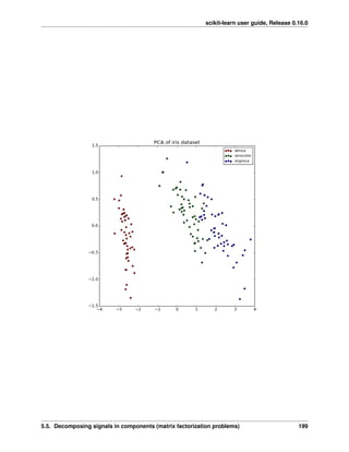
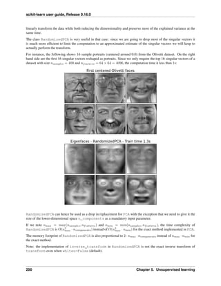

![scikit-learn user guide, Release 0.16.0
Mini-batch sparse PCA (MiniBatchSparsePCA) is a variant of SparsePCA that is faster but less accurate. The
increased speed is reached by iterating over small chunks of the set of features, for a given number of iterations.
Principal component analysis (PCA) has the disadvantage that the components extracted by this method have exclu-
sively dense expressions, i.e. they have non-zero coefficients when expressed as linear combinations of the original
variables. This can make interpretation difficult. In many cases, the real underlying components can be more naturally
imagined as sparse vectors; for example in face recognition, components might naturally map to parts of faces.
Sparse principal components yields a more parsimonious, interpretable representation, clearly emphasizing which of
the original features contribute to the differences between samples.
The following example illustrates 16 components extracted using sparse PCA from the Olivetti faces dataset. It can
be seen how the regularization term induces many zeros. Furthermore, the natural structure of the data causes the
non-zero coefficients to be vertically adjacent. The model does not enforce this mathematically: each component is
a vector ℎ ∈ R4096
, and there is no notion of vertical adjacency except during the human-friendly visualization as
64x64 pixel images. The fact that the components shown below appear local is the effect of the inherent structure of
the data, which makes such local patterns minimize reconstruction error. There exist sparsity-inducing norms that take
into account adjacency and different kinds of structure; see [Jen09] for a review of such methods. For more details on
how to use Sparse PCA, see the Examples section, below.
Note that there are many different formulations for the Sparse PCA problem. The one implemented here is based
on [Mrl09] . The optimization problem solved is a PCA problem (dictionary learning) with an ℓ1 penalty on the
202 Chapter 5. Unsupervised learning](https://image.slidesharecdn.com/scikit-learn0-150409112902-conversion-gate01/85/Scikit-learn-0-16-0-user-guide-212-320.jpg)

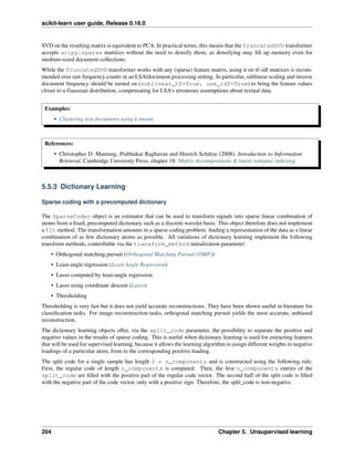


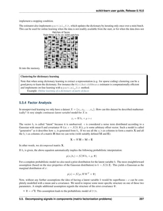


![scikit-learn user guide, Release 0.16.0
Examples:
• Blind source separation using FastICA
• FastICA on 2D point clouds
• Faces dataset decompositions
5.5.6 Non-negative matrix factorization (NMF or NNMF)
NMF is an alternative approach to decomposition that assumes that the data and the components are non-negative. NMF
can be plugged in instead of PCA or its variants, in the cases where the data matrix does not contain negative values.
It finds a decomposition of samples 𝑋 into two matrices 𝑊 and 𝐻 of non-negative elements, by optimizing for the
squared Frobenius norm:
arg min
𝑊,𝐻
||𝑋 − 𝑊 𝐻||2
=
∑︁
𝑖,𝑗
𝑋𝑖𝑗 − 𝑊 𝐻 𝑖𝑗
This norm is an obvious extension of the Euclidean norm to matrices. (Other optimization objectives have been
suggested in the NMF literature, in particular Kullback-Leibler divergence, but these are not currently implemented.)
Unlike PCA, the representation of a vector is obtained in an additive fashion, by superimposing the components,
without subtracting. Such additive models are efficient for representing images and text.
It has been observed in [Hoyer, 04] that, when carefully constrained, NMF can produce a parts-based representation of
the dataset, resulting in interpretable models. The following example displays 16 sparse components found by NMF
from the images in the Olivetti faces dataset, in comparison with the PCA eigenfaces.
5.5. Decomposing signals in components (matrix factorization problems) 211](https://image.slidesharecdn.com/scikit-learn0-150409112902-conversion-gate01/85/Scikit-learn-0-16-0-user-guide-221-320.jpg)


![scikit-learn user guide, Release 0.16.0
whether the data are centered or not, the result will be different, so one may want to use the assume_centered
parameter accurately.
Mathematically, this shrinkage consists in reducing the ratio between the smallest and the largest eigenvalue of the
empirical covariance matrix. It can be done by simply shifting every eigenvalue according to a given offset, which is
equivalent of finding the l2-penalized Maximum Likelihood Estimator of the covariance matrix. In practice, shrinkage
boils down to a simple a convex transformation : Σshrunk = (1 − 𝛼)ˆΣ + 𝛼Tr^Σ
𝑝 Id.
Choosing the amount of shrinkage, 𝛼 amounts to setting a bias/variance trade-off, and is discussed below.
Examples:
• See Shrinkage covariance estimation: LedoitWolf vs OAS and max-likelihood for an example on how to
fit a ShrunkCovariance object to data.
Ledoit-Wolf shrinkage
In their 2004 paper [1], O. Ledoit and M. Wolf propose a formula so as to compute the optimal shrinkage coefficient
𝛼 that minimizes the Mean Squared Error between the estimated and the real covariance matrix.
The Ledoit-Wolf estimator of the covariance matrix can be computed on a sample with the ledoit_wolf function of
the sklearn.covariance package, or it can be otherwise obtained by fitting a LedoitWolf object to the same sample.
Examples:
• See Shrinkage covariance estimation: LedoitWolf vs OAS and max-likelihood for an example on how to fit
a LedoitWolf object to data and for visualizing the performances of the Ledoit-Wolf estimator in terms
of likelihood.
[1] O. Ledoit and M. Wolf, “A Well-Conditioned Estimator for Large-Dimensional Covariance Matrices”, Jour-
nal of Multivariate Analysis, Volume 88, Issue 2, February 2004, pages 365-411.
Oracle Approximating Shrinkage
Under the assumption that the data are Gaussian distributed, Chen et al. [2] derived a formula aimed at choosing a
shrinkage coefficient that yields a smaller Mean Squared Error than the one given by Ledoit and Wolf’s formula. The
resulting estimator is known as the Oracle Shrinkage Approximating estimator of the covariance.
The OAS estimator of the covariance matrix can be computed on a sample with the oas function of the
sklearn.covariance package, or it can be otherwise obtained by fitting an OAS object to the same sample.
[2] Chen et al., “Shrinkage Algorithms for MMSE Covariance Estimation”, IEEE Trans. on Sign. Proc., Volume
58, Issue 10, October 2010.
Examples:
• See Shrinkage covariance estimation: LedoitWolf vs OAS and max-likelihood for an example on how to
fit an OAS object to data.
• See Ledoit-Wolf vs OAS estimation to visualize the Mean Squared Error difference between a
LedoitWolf and an OAS estimator of the covariance.
214 Chapter 5. Unsupervised learning](https://image.slidesharecdn.com/scikit-learn0-150409112902-conversion-gate01/85/Scikit-learn-0-16-0-user-guide-224-320.jpg)

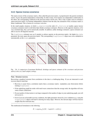
![scikit-learn user guide, Release 0.16.0
Where 𝐾 is the precision matrix to be estimated, and 𝑆 is the sample covariance matrix. ‖𝐾‖1 is the sum of the abso-
lute values of off-diagonal coefficients of 𝐾. The algorithm employed to solve this problem is the GLasso algorithm,
from the Friedman 2008 Biostatistics paper. It is the same algorithm as in the R glasso package.
Examples:
• Sparse inverse covariance estimation: example on synthetic data showing some recovery of a structure,
and comparing to other covariance estimators.
• Visualizing the stock market structure: example on real stock market data, finding which symbols are most
linked.
References:
• Friedman et al, “Sparse inverse covariance estimation with the graphical lasso”, Biostatistics 9, pp 432,
2008
5.6.4 Robust Covariance Estimation
Real data set are often subjects to measurement or recording errors. Regular but uncommon observations may also
appear for a variety of reason. Every observation which is very uncommon is called an outlier. The empirical covari-
ance estimator and the shrunk covariance estimators presented above are very sensitive to the presence of outlying
observations in the data. Therefore, one should use robust covariance estimators to estimate the covariance of its real
data sets. Alternatively, robust covariance estimators can be used to perform outlier detection and discard/downweight
some observations according to further processing of the data.
The sklearn.covariance package implements a robust estimator of covariance, the Minimum Covariance De-
terminant [3].
Minimum Covariance Determinant
The Minimum Covariance Determinant estimator is a robust estimator of a data set’s covariance introduced by P.J.
Rousseeuw in [3]. The idea is to find a given proportion (h) of “good” observations which are not outliers and
compute their empirical covariance matrix. This empirical covariance matrix is then rescaled to compensate the
performed selection of observations (“consistency step”). Having computed the Minimum Covariance Determinant
estimator, one can give weights to observations according to their Mahalanobis distance, leading the a reweighted
estimate of the covariance matrix of the data set (“reweighting step”).
Rousseeuw and Van Driessen [4] developed the FastMCD algorithm in order to compute the Minimum Covariance
Determinant. This algorithm is used in scikit-learn when fitting an MCD object to data. The FastMCD algorithm also
computes a robust estimate of the data set location at the same time.
Raw estimates can be accessed as raw_location_ and raw_covariance_ attributes of a MinCovDet robust
covariance estimator object.
[3] P. J. Rousseeuw. Least median of squares regression.
10. Am Stat Ass, 79:871, 1984.
[4] A Fast Algorithm for the Minimum Covariance Determinant Estimator, 1999, American Statistical Associa-
tion and the American Society for Quality, TECHNOMETRICS.
5.6. Covariance estimation 217](https://image.slidesharecdn.com/scikit-learn0-150409112902-conversion-gate01/85/Scikit-learn-0-16-0-user-guide-227-320.jpg)


![scikit-learn user guide, Release 0.16.0
It’s clear how the kernel shape affects the smoothness of the resulting distribution. The scikit-learn kernel density
estimator can be used as follows:
>>> from sklearn.neighbors.kde import KernelDensity
>>> import numpy as np
>>> X = np.array([[-1, -1], [-2, -1], [-3, -2], [1, 1], [2, 1], [3, 2]])
>>> kde = KernelDensity(kernel='gaussian', bandwidth=0.2).fit(X)
>>> kde.score_samples(X)
array([-0.41075698, -0.41075698, -0.41076071, -0.41075698, -0.41075698,
-0.41076071])
Here we have used kernel=’gaussian’, as seen above. Mathematically, a kernel is a positive function 𝐾(𝑥; ℎ)
which is controlled by the bandwidth parameter ℎ. Given this kernel form, the density estimate at a point 𝑦 within a
group of points 𝑥𝑖; 𝑖 = 1 · · · 𝑁 is given by:
𝜌 𝐾(𝑦) =
𝑁∑︁
𝑖=1
𝐾((𝑦 − 𝑥𝑖)/ℎ)
The bandwidth here acts as a smoothing parameter, controlling the tradeoff between bias and variance in the result. A
large bandwidth leads to a very smooth (i.e. high-bias) density distribution. A small bandwidth leads to an unsmooth
(i.e. high-variance) density distribution.
sklearn.neighbors.KernelDensity implements several common kernel forms, which are shown in the fol-
lowing figure:
5.8. Density Estimation 223](https://image.slidesharecdn.com/scikit-learn0-150409112902-conversion-gate01/85/Scikit-learn-0-16-0-user-guide-233-320.jpg)
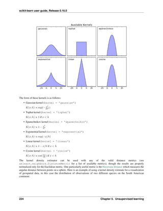


![scikit-learn user guide, Release 0.16.0
sets.
A solution to this problem is a procedure called cross-validation (CV for short). A test set should still be held out for
final evaluation, but the validation set is no longer needed when doing CV. In the basic approach, called k-fold CV, the
training set is split into k smaller sets (other approaches are described below, but generally follow the same principles).
The following procedure is followed for each of the k “folds”:
• A model is trained using 𝑘 − 1 of the folds as training data;
• the resulting model is validated on the remaining part of the data (i.e., it is used as a test set to compute a
performance measure such as accuracy).
The performance measure reported by k-fold cross-validation is then the average of the values computed in the loop.
This approach can be computationally expensive, but does not waste too much data (as it is the case when fixing an
arbitrary test set), which is a major advantage in problem such as inverse inference where the number of samples is
very small.
6.1.1 Computing cross-validated metrics
The simplest way to use cross-validation is to call the cross_val_score helper function on the estimator and the
dataset.
The following example demonstrates how to estimate the accuracy of a linear kernel support vector machine on the
iris dataset by splitting the data, fitting a model and computing the score 5 consecutive times (with different splits each
time):
>>> clf = svm.SVC(kernel='linear', C=1)
>>> scores = cross_validation.cross_val_score(
... clf, iris.data, iris.target, cv=5)
...
>>> scores
array([ 0.96..., 1. ..., 0.96..., 0.96..., 1. ])
The mean score and the 95% confidence interval of the score estimate are hence given by:
>>> print("Accuracy: %0.2f (+/- %0.2f)" % (scores.mean(), scores.std() * 2))
Accuracy: 0.98 (+/- 0.03)
By default, the score computed at each CV iteration is the score method of the estimator. It is possible to change
this by using the scoring parameter:
>>> from sklearn import metrics
>>> scores = cross_validation.cross_val_score(clf, iris.data, iris.target,
... cv=5, scoring='f1_weighted')
>>> scores
array([ 0.96..., 1. ..., 0.96..., 0.96..., 1. ])
See The scoring parameter: defining model evaluation rules for details. In the case of the Iris dataset, the samples are
balanced across target classes hence the accuracy and the F1-score are almost equal.
When the cv argument is an integer, cross_val_score uses the KFold or StratifiedKFold strategies by
default, the latter being used if the estimator derives from ClassifierMixin.
It is also possible to use other cross validation strategies by passing a cross validation iterator instead, for instance:
>>> n_samples = iris.data.shape[0]
>>> cv = cross_validation.ShuffleSplit(n_samples, n_iter=3,
... test_size=0.3, random_state=0)
>>> cross_validation.cross_val_score(clf, iris.data, iris.target, cv=cv)
230 Chapter 6. Model selection and evaluation](https://image.slidesharecdn.com/scikit-learn0-150409112902-conversion-gate01/85/Scikit-learn-0-16-0-user-guide-240-320.jpg)
![scikit-learn user guide, Release 0.16.0
...
array([ 0.97..., 0.97..., 1. ])
Data transformation with held out data
Just as it is important to test a predictor on data held-out from training, preprocessing (such as standardization,
feature selection, etc.) and similar data transformations similarly should be learnt from a training set and applied
to held-out data for prediction:
>>> from sklearn import preprocessing
>>> X_train, X_test, y_train, y_test = cross_validation.train_test_split(
... iris.data, iris.target, test_size=0.4, random_state=0)
>>> scaler = preprocessing.StandardScaler().fit(X_train)
>>> X_train_transformed = scaler.transform(X_train)
>>> clf = svm.SVC(C=1).fit(X_train_transformed, y_train)
>>> X_test_transformed = scaler.transform(X_test)
>>> clf.score(X_test_transformed, y_test)
0.9333...
A Pipeline makes it easier to compose estimators, providing this behavior under cross-validation:
>>> from sklearn.pipeline import make_pipeline
>>> clf = make_pipeline(preprocessing.StandardScaler(), svm.SVC(C=1))
>>> cross_validation.cross_val_score(clf, iris.data, iris.target, cv=cv)
...
array([ 0.97..., 0.93..., 0.95...])
See Pipeline and FeatureUnion: combining estimators.
Obtaining predictions by cross-validation
The function cross_val_predict has a similar interface to cross_val_score, but returns, for each element
in the input, the prediction that was obtained for that element when it was in the test set. Only cross-validation
strategies that assign all elements to a test set exactly once can be used (otherwise, an exception is raised).
These prediction can then be used to evaluate the classifier:
>>> predicted = cross_validation.cross_val_predict(clf, iris.data,
... iris.target, cv=10)
>>> metrics.accuracy_score(iris.target, predicted)
0.966...
Note that the result of this computation may be slightly different from those obtained using cross_val_score as
the elements are grouped in different ways.
The available cross validation iterators are introduced in the following section.
Examples
• Receiver Operating Characteristic (ROC) with cross validation,
• Recursive feature elimination with cross-validation,
• Parameter estimation using grid search with cross-validation,
• Sample pipeline for text feature extraction and evaluation,
• Plotting Cross-Validated Predictions,
6.1. Cross-validation: evaluating estimator performance 231](https://image.slidesharecdn.com/scikit-learn0-150409112902-conversion-gate01/85/Scikit-learn-0-16-0-user-guide-241-320.jpg)
![scikit-learn user guide, Release 0.16.0
6.1.2 Cross validation iterators
The following sections list utilities to generate indices that can be used to generate dataset splits according to different
cross validation strategies.
K-fold
KFold divides all the samples in 𝑘 groups of samples, called folds (if 𝑘 = 𝑛, this is equivalent to the Leave One Out
strategy), of equal sizes (if possible). The prediction function is learned using 𝑘 − 1 folds, and the fold left out is used
for test.
Example of 2-fold cross-validation on a dataset with 4 samples:
>>> import numpy as np
>>> from sklearn.cross_validation import KFold
>>> kf = KFold(4, n_folds=2)
>>> for train, test in kf:
... print("%s %s" % (train, test))
[2 3] [0 1]
[0 1] [2 3]
Each fold is constituted by two arrays: the first one is related to the training set, and the second one to the test set.
Thus, one can create the training/test sets using numpy indexing:
>>> X = np.array([[0., 0.], [1., 1.], [-1., -1.], [2., 2.]])
>>> y = np.array([0, 1, 0, 1])
>>> X_train, X_test, y_train, y_test = X[train], X[test], y[train], y[test]
Stratified k-fold
StratifiedKFold is a variation of k-fold which returns stratified folds: each set contains approximately the same
percentage of samples of each target class as the complete set.
Example of stratified 2-fold cross-validation on a dataset with 10 samples from two slightly unbalanced classes:
>>> from sklearn.cross_validation import StratifiedKFold
>>> labels = [0, 0, 0, 0, 1, 1, 1, 1, 1, 1]
>>> skf = StratifiedKFold(labels, 3)
>>> for train, test in skf:
... print("%s %s" % (train, test))
[2 3 6 7 8 9] [0 1 4 5]
[0 1 3 4 5 8 9] [2 6 7]
[0 1 2 4 5 6 7] [3 8 9]
Leave-One-Out - LOO
LeaveOneOut (or LOO) is a simple cross-validation. Each learning set is created by taking all the samples except
one, the test set being the sample left out. Thus, for 𝑛 samples, we have 𝑛 different training sets and 𝑛 different tests
set. This cross-validation procedure does not waste much data as only one sample is removed from the training set:
>>> from sklearn.cross_validation import LeaveOneOut
>>> loo = LeaveOneOut(4)
232 Chapter 6. Model selection and evaluation](https://image.slidesharecdn.com/scikit-learn0-150409112902-conversion-gate01/85/Scikit-learn-0-16-0-user-guide-242-320.jpg)
![scikit-learn user guide, Release 0.16.0
>>> for train, test in loo:
... print("%s %s" % (train, test))
[1 2 3] [0]
[0 2 3] [1]
[0 1 3] [2]
[0 1 2] [3]
Potential users of LOO for model selection should weigh a few known caveats. When compared with 𝑘-fold cross
validation, one builds 𝑛 models from 𝑛 samples instead of 𝑘 models, where 𝑛 > 𝑘. Moreover, each is trained on 𝑛 − 1
samples rather than (𝑘 − 1)𝑛/𝑘. In both ways, assuming 𝑘 is not too large and 𝑘 < 𝑛, LOO is more computationally
expensive than 𝑘-fold cross validation.
In terms of accuracy, LOO often results in high variance as an estimator for the test error. Intuitively, since 𝑛 − 1 of
the 𝑛 samples are used to build each model, models constructed from folds are virtually identical to each other and to
the model built from the entire training set.
However, if the learning curve is steep for the training size in question, then 5- or 10- fold cross validation can
overestimate the generalization error.
As a general rule, most authors, and empirical evidence, suggest that 5- or 10- fold cross validation should be preferred
to LOO.
References:
• http://www.faqs.org/faqs/ai-faq/neural-nets/part3/section-12.html
• T. Hastie, R. Tibshirani, J. Friedman, The Elements of Statistical Learning, Springer 2009
• L. Breiman, P. Spector Submodel selection and evaluation in regression: The X-random case, International
Statistical Review 1992
• R. Kohavi, A Study of Cross-Validation and Bootstrap for Accuracy Estimation and Model Selection, Intl.
Jnt. Conf. AI
• R. Bharat Rao, G. Fung, R. Rosales, On the Dangers of Cross-Validation. An Experimental Evaluation,
SIAM 2008
• G. James, D. Witten, T. Hastie, R Tibshirani, An Introduction to Statistical Learning, Springer 2013
Leave-P-Out - LPO
LeavePOut is very similar to LeaveOneOut as it creates all the possible training/test sets by removing 𝑝 samples
from the complete set. For 𝑛 samples, this produces
(︀ 𝑛
𝑝
)︀
train-test pairs. Unlike LeaveOneOut and KFold, the test
sets will overlap for 𝑝 > 1.
Example of Leave-2-Out on a dataset with 4 samples:
>>> from sklearn.cross_validation import LeavePOut
>>> lpo = LeavePOut(4, p=2)
>>> for train, test in lpo:
... print("%s %s" % (train, test))
[2 3] [0 1]
[1 3] [0 2]
[1 2] [0 3]
[0 3] [1 2]
[0 2] [1 3]
[0 1] [2 3]
6.1. Cross-validation: evaluating estimator performance 233](https://image.slidesharecdn.com/scikit-learn0-150409112902-conversion-gate01/85/Scikit-learn-0-16-0-user-guide-243-320.jpg)
![scikit-learn user guide, Release 0.16.0
Leave-One-Label-Out - LOLO
LeaveOneLabelOut (LOLO) is a cross-validation scheme which holds out the samples according to a third-party
provided array of integer labels. This label information can be used to encode arbitrary domain specific pre-defined
cross-validation folds.
Each training set is thus constituted by all the samples except the ones related to a specific label.
For example, in the cases of multiple experiments, LOLO can be used to create a cross-validation based on the different
experiments: we create a training set using the samples of all the experiments except one:
>>> from sklearn.cross_validation import LeaveOneLabelOut
>>> labels = [1, 1, 2, 2]
>>> lolo = LeaveOneLabelOut(labels)
>>> for train, test in lolo:
... print("%s %s" % (train, test))
[2 3] [0 1]
[0 1] [2 3]
Another common application is to use time information: for instance the labels could be the year of collection of the
samples and thus allow for cross-validation against time-based splits.
Warning: Contrary to StratifiedKFold, the ‘‘labels‘‘ of :class:‘LeaveOneLabelOut‘ should not encode
the target class to predict: the goal of StratifiedKFold is to rebalance dataset classes across the train / test
split to ensure that the train and test folds have approximately the same percentage of samples of each class while
LeaveOneLabelOut will do the opposite by ensuring that the samples of the train and test fold will not share
the same label value.
Leave-P-Label-Out
LeavePLabelOut is similar as Leave-One-Label-Out, but removes samples related to 𝑃 labels for each training/test
set.
Example of Leave-2-Label Out:
>>> from sklearn.cross_validation import LeavePLabelOut
>>> labels = [1, 1, 2, 2, 3, 3]
>>> lplo = LeavePLabelOut(labels, p=2)
>>> for train, test in lplo:
... print("%s %s" % (train, test))
[4 5] [0 1 2 3]
[2 3] [0 1 4 5]
[0 1] [2 3 4 5]
Random permutations cross-validation a.k.a. Shuffle & Split
ShuffleSplit
The ShuffleSplit iterator will generate a user defined number of independent train / test dataset splits. Samples
are first shuffled and then split into a pair of train and test sets.
It is possible to control the randomness for reproducibility of the results by explicitly seeding the random_state
pseudo random number generator.
Here is a usage example:
234 Chapter 6. Model selection and evaluation](https://image.slidesharecdn.com/scikit-learn0-150409112902-conversion-gate01/85/Scikit-learn-0-16-0-user-guide-244-320.jpg)
![scikit-learn user guide, Release 0.16.0
>>> ss = cross_validation.ShuffleSplit(5, n_iter=3, test_size=0.25,
... random_state=0)
>>> for train_index, test_index in ss:
... print("%s %s" % (train_index, test_index))
...
[1 3 4] [2 0]
[1 4 3] [0 2]
[4 0 2] [1 3]
ShuffleSplit is thus a good alternative to KFold cross validation that allows a finer control on the number of
iterations and the proportion of samples in on each side of the train / test split.
Predefined Fold-Splits / Validation-Sets
For some datasets, a pre-defined split of the data into training- and validation fold or into several cross-validation folds
already exists. Using PredefinedSplit it is possible to use these folds e.g. when searching for hyperparameters.
For example, when using a validation set, set the test_fold to 0 for all samples that are part of the validation set,
and to -1 for all other samples.
See also
StratifiedShuffleSplit is a variation of ShuffleSplit, which returns stratified splits, i.e which creates splits
by preserving the same percentage for each target class as in the complete set.
6.1.3 A note on shuffling
If the data ordering is not arbitrary (e.g. samples with the same label are contiguous), shuffling it first may be essential
to get a meaningful cross- validation result. However, the opposite may be true if the samples are not independently
and identically distributed. For example, if samples correspond to news articles, and are ordered by their time of
publication, then shuffling the data will likely lead to a model that is overfit and an inflated validation score: it will be
tested on samples that are artificially similar (close in time) to training samples.
Some cross validation iterators, such as KFold, have an inbuilt option to shuffle the data indices before splitting them.
Note that:
• This consumes less memory than shuffling the data directly.
• By default no shuffling occurs, including for the (stratified) K fold cross- validation performed by specifying
cv=some_integer to cross_val_score, grid search, etc. Keep in mind that train_test_split
still returns a random split.
• The random_state parameter defaults to None, meaning that the shuffling will be different every time
KFold(..., shuffle=True) is iterated. However, GridSearchCV will use the same shuffling for
each set of parameters validated by a single call to its fit method.
• To ensure results are repeatable (on the same platform), use a fixed value for random_state.
6.1.4 Cross validation and model selection
Cross validation iterators can also be used to directly perform model selection using Grid Search for the optimal
hyperparameters of the model. This is the topic if the next section: Grid Search: Searching for estimator parameters.
6.1. Cross-validation: evaluating estimator performance 235](https://image.slidesharecdn.com/scikit-learn0-150409112902-conversion-gate01/85/Scikit-learn-0-16-0-user-guide-245-320.jpg)
![scikit-learn user guide, Release 0.16.0
6.2 Grid Search: Searching for estimator parameters
Parameters that are not directly learnt within estimators can be set by searching a parameter space for the best Cross-
validation: evaluating estimator performance score. Typical examples include C, kernel and gamma for Support
Vector Classifier, alpha for Lasso, etc.
Any parameter provided when constructing an estimator may be optimized in this manner. Specifically, to find the
names and current values for all parameters for a given estimator, use:
estimator.get_params()
Such parameters are often referred to as hyperparameters (particularly in Bayesian learning), distinguishing them from
the parameters optimised in a machine learning procedure.
A search consists of:
• an estimator (regressor or classifier such as sklearn.svm.SVC());
• a parameter space;
• a method for searching or sampling candidates;
• a cross-validation scheme; and
• a score function.
Some models allow for specialized, efficient parameter search strategies, outlined below. Two generic approaches to
sampling search candidates are provided in scikit-learn: for given values, GridSearchCV exhaustively considers all
parameter combinations, while RandomizedSearchCV can sample a given number of candidates from a parameter
space with a specified distribution. After describing these tools we detail best practice applicable to both approaches.
6.2.1 Exhaustive Grid Search
The grid search provided by GridSearchCV exhaustively generates candidates from a grid of parameter values
specified with the param_grid parameter. For instance, the following param_grid:
param_grid = [
{'C': [1, 10, 100, 1000], 'kernel': ['linear']},
{'C': [1, 10, 100, 1000], 'gamma': [0.001, 0.0001], 'kernel': ['rbf']},
]
specifies that two grids should be explored: one with a linear kernel and C values in [1, 10, 100, 1000], and the second
one with an RBF kernel, and the cross-product of C values ranging in [1, 10, 100, 1000] and gamma values in [0.001,
0.0001].
The GridSearchCV instance implements the usual estimator API: when “fitting” it on a dataset all the possible
combinations of parameter values are evaluated and the best combination is retained.
Examples:
• See Parameter estimation using grid search with cross-validation for an example of Grid Search compu-
tation on the digits dataset.
• See Sample pipeline for text feature extraction and evaluation for an example of Grid Search coupling
parameters from a text documents feature extractor (n-gram count vectorizer and TF-IDF transformer)
with a classifier (here a linear SVM trained with SGD with either elastic net or L2 penalty) using a
pipeline.Pipeline instance.
236 Chapter 6. Model selection and evaluation](https://image.slidesharecdn.com/scikit-learn0-150409112902-conversion-gate01/85/Scikit-learn-0-16-0-user-guide-246-320.jpg)
![scikit-learn user guide, Release 0.16.0
6.2.2 Randomized Parameter Optimization
While using a grid of parameter settings is currently the most widely used method for parameter optimization, other
search methods have more favourable properties. RandomizedSearchCV implements a randomized search over
parameters, where each setting is sampled from a distribution over possible parameter values. This has two main
benefits over an exhaustive search:
• A budget can be chosen independent of the number of parameters and possible values.
• Adding parameters that do not influence the performance does not decrease efficiency.
Specifying how parameters should be sampled is done using a dictionary, very similar to specifying parameters for
GridSearchCV. Additionally, a computation budget, being the number of sampled candidates or sampling itera-
tions, is specified using the n_iter parameter. For each parameter, either a distribution over possible values or a list
of discrete choices (which will be sampled uniformly) can be specified:
[{'C': scipy.stats.expon(scale=100), 'gamma': scipy.stats.expon(scale=.1),
'kernel': ['rbf'], 'class_weight':['auto', None]}]
This example uses the scipy.stats module, which contains many useful distributions for sampling parameters,
such as expon, gamma, uniform or randint. In principle, any function can be passed that provides a rvs
(random variate sample) method to sample a value. A call to the rvs function should provide independent random
samples from possible parameter values on consecutive calls.
Warning: The distributions in scipy.stats do not allow specifying a random state. Instead,
they use the global numpy random state, that can be seeded via np.random.seed or set using
np.random.set_state.
For continuous parameters, such as C above, it is important to specify a continuous distribution to take full advantage
of the randomization. This way, increasing n_iter will always lead to a finer search.
Examples:
• Comparing randomized search and grid search for hyperparameter estimation compares the usage and
efficiency of randomized search and grid search.
References:
• Bergstra, J. and Bengio, Y., Random search for hyper-parameter optimization, The Journal of Machine
Learning Research (2012)
6.2.3 Tips for parameter search
Specifying an objective metric
By default, parameter search uses the score function of the estimator to evaluate a parameter setting. These are
the sklearn.metrics.accuracy_score for classification and sklearn.metrics.r2_score for regres-
sion. For some applications, other scoring functions are better suited (for example in unbalanced classification, the
accuracy score is often uninformative). An alternative scoring function can be specified via the scoring parameter
to GridSearchCV, RandomizedSearchCV and many of the specialized cross-validation tools described below.
See The scoring parameter: defining model evaluation rules for more details.
6.2. Grid Search: Searching for estimator parameters 237](https://image.slidesharecdn.com/scikit-learn0-150409112902-conversion-gate01/85/Scikit-learn-0-16-0-user-guide-247-320.jpg)


![scikit-learn user guide, Release 0.16.0
Scoring Function Comment
Classification
‘accuracy’ metrics.accuracy_score
‘average_precision’ metrics.average_precision_score
‘f1’ metrics.f1_score for binary targets
‘f1_micro’ metrics.f1_score micro-averaged
‘f1_macro’ metrics.f1_score macro-averaged
‘f1_weighted’ metrics.f1_score weighted average
‘f1_samples’ metrics.f1_score by multilabel sample
‘log_loss’ metrics.log_loss requires predict_proba support
‘precision’ etc. metrics.precision_score suffixes apply as with ‘f1’
‘recall’ etc. metrics.recall_score suffixes apply as with ‘f1’
‘roc_auc’ metrics.roc_auc_score
Clustering
‘adjusted_rand_score’ metrics.adjusted_rand_score
Regression
‘mean_absolute_error’ metrics.mean_absolute_error
‘mean_squared_error’ metrics.mean_squared_error
‘median_absolute_error’ metrics.median_absolute_error
‘r2’ metrics.r2_score
Usage examples:
>>> from sklearn import svm, cross_validation, datasets
>>> iris = datasets.load_iris()
>>> X, y = iris.data, iris.target
>>> model = svm.SVC()
>>> cross_validation.cross_val_score(model, X, y, scoring='wrong_choice')
Traceback (most recent call last):
ValueError: 'wrong_choice' is not a valid scoring value. Valid options are ['accuracy', 'adjusted_ran
>>> clf = svm.SVC(probability=True, random_state=0)
>>> cross_validation.cross_val_score(clf, X, y, scoring='log_loss')
array([-0.07..., -0.16..., -0.06...])
Note: The values listed by the ValueError exception correspond to the functions measuring prediction accu-
racy described in the following sections. The scorer objects for those functions are stored in the dictionary
sklearn.metrics.SCORERS.
Defining your scoring strategy from metric functions
The module sklearn.metric also exposes a set of simple functions measuring a prediction error given ground
truth and prediction:
• functions ending with _score return a value to maximize, the higher the better.
• functions ending with _error or _loss return a value to minimize, the lower the better. When converting into
a scorer object using make_scorer, set the greater_is_better parameter to False (True by default; see
the parameter description below).
Metrics available for various machine learning tasks are detailed in sections below.
Many metrics are not given names to be used as scoring values, sometimes because they require additional param-
eters, such as fbeta_score. In such cases, you need to generate an appropriate scoring object. The simplest way
to generate a callable object for scoring is by using make_scorer. That function converts metrics into callables that
can be used for model evaluation.
240 Chapter 6. Model selection and evaluation](https://image.slidesharecdn.com/scikit-learn0-150409112902-conversion-gate01/85/Scikit-learn-0-16-0-user-guide-250-320.jpg)
![scikit-learn user guide, Release 0.16.0
One typical use case is to wrap an existing metric function from the library with non-default values for its parameters,
such as the beta parameter for the fbeta_score function:
>>> from sklearn.metrics import fbeta_score, make_scorer
>>> ftwo_scorer = make_scorer(fbeta_score, beta=2)
>>> from sklearn.grid_search import GridSearchCV
>>> from sklearn.svm import LinearSVC
>>> grid = GridSearchCV(LinearSVC(), param_grid={'C': [1, 10]}, scoring=ftwo_scorer)
The second use case is to build a completely custom scorer object from a simple python function using
make_scorer, which can take several parameters:
• the python function you want to use (my_custom_loss_func in the example below)
• whether the python function returns a score (greater_is_better=True, the default) or a loss
(greater_is_better=False). If a loss, the output of the python function is negated by the scorer ob-
ject, conforming to the cross validation convention that scorers return higher values for better models.
• for classification metrics only: whether the python function you provided requires continuous decision certain-
ties (needs_threshold=True). The default value is False.
• any additional parameters, such as beta in an f1_score.
Here is an example of building custom scorers, and of using the greater_is_better parameter:
>>> import numpy as np
>>> def my_custom_loss_func(ground_truth, predictions):
... diff = np.abs(ground_truth - predictions).max()
... return np.log(1 + diff)
...
>>> # loss_func will negate the return value of my_custom_loss_func,
>>> # which will be np.log(2), 0.693, given the values for ground_truth
>>> # and predictions defined below.
>>> loss = make_scorer(my_custom_loss_func, greater_is_better=False)
>>> score = make_scorer(my_custom_loss_func, greater_is_better=True)
>>> ground_truth = [1, 1]
>>> predictions = [0, 1]
>>> from sklearn.dummy import DummyClassifier
>>> clf = DummyClassifier(strategy='most_frequent', random_state=0)
>>> clf = clf.fit(ground_truth, predictions)
>>> loss(clf,ground_truth, predictions)
-0.69...
>>> score(clf,ground_truth, predictions)
0.69...
Implementing your own scoring object
You can generate even more flexible model scorers by constructing your own scoring object from scratch, without using
the make_scorer factory. For a callable to be a scorer, it needs to meet the protocol specified by the following two
rules:
• It can be called with parameters (estimator, X, y), where estimator is the model that should be
evaluated, X is validation data, and y is the ground truth target for X (in the supervised case) or None (in the
unsupervised case).
• It returns a floating point number that quantifies the estimator prediction quality on X, with reference to y.
Again, by convention higher numbers are better, so if your scorer returns loss, that value should be negated.
6.3. Model evaluation: quantifying the quality of predictions 241](https://image.slidesharecdn.com/scikit-learn0-150409112902-conversion-gate01/85/Scikit-learn-0-16-0-user-guide-251-320.jpg)
![scikit-learn user guide, Release 0.16.0
6.3.2 Classification metrics
The sklearn.metrics module implements several loss, score, and utility functions to measure classification per-
formance. Some metrics might require probability estimates of the positive class, confidence values, or binary deci-
sions values. Most implementations allow each sample to provide a weighted contribution to the overall score, through
the sample_weight parameter.
Some of these are restricted to the binary classification case:
Others also work in the multiclass case:
Some also work in the multilabel case:
And some work with binary and multilabel (but not multiclass) problems:
In the following sub-sections, we will describe each of those functions, preceded by some notes on common API and
metric definition.
From binary to multiclass and multilabel
Some metrics are essentially defined for binary classification tasks (e.g. f1_score, roc_auc_score). In these
cases, by default only the positive label is evaluated, assuming by default that the positive class is labelled 1 (though
this may be configurable through the pos_label parameter). In extending a binary metric to multiclass or multilabel
problems, the data is treated as a collection of binary problems, one for each class. There are then a number of ways
to average binary metric calculations across the set of classes, each of which may be useful in some scenario. Where
available, you should select among these using the average parameter.
• "macro" simply calculates the mean of the binary metrics, giving equal weight to each class. In problems
where infrequent classes are nonetheless important, macro-averaging may be a means of highlighting their
performance. On the other hand, the assumption that all classes are equally important is often untrue, such that
macro-averaging will over-emphasize the typically low performance on an infrequent class.
• "weighted" accounts for class imbalance by computing the average of binary metrics in which each class’s
score is weighted by its presence in the true data sample.
• "micro" gives each sample-class pair an equal contribution to the overall metric (except as a result of sample-
weight). Rather than summing the metric per class, this sums the dividends and divisors that make up the
the per-class metrics to calculate an overall quotient. Micro-averaging may be preferred in multilabel settings,
including multiclass classification where a majority class is to be ignored.
• "samples" applies only to multilabel problems. It does not calculate a per-class measure, instead calculat-
ing the metric over the true and predicted classes for each sample in the evaluation data, and returning their
(sample_weight-weighted) average.
• Selecting average=None will return an array with the score for each class.
While multiclass data is provided to the metric, like binary targets, as an array of class labels, multilabel data is
specified as an indicator matrix, in which cell [i, j] has value 1 if sample i has label j and value 0 otherwise.
242 Chapter 6. Model selection and evaluation](https://image.slidesharecdn.com/scikit-learn0-150409112902-conversion-gate01/85/Scikit-learn-0-16-0-user-guide-252-320.jpg)
![scikit-learn user guide, Release 0.16.0
Accuracy score
The accuracy_score function computes the accuracy, either the fraction (default) or the count (normalize=False)
of correct predictions.
In multilabel classification, the function returns the subset accuracy. If the entire set of predicted labels for a sample
strictly match with the true set of labels, then the subset accuracy is 1.0; otherwise it is 0.0.
If ˆ𝑦𝑖 is the predicted value of the 𝑖-th sample and 𝑦𝑖 is the corresponding true value, then the fraction of correct
predictions over 𝑛samples is defined as
accuracy(𝑦, ˆ𝑦) =
1
𝑛samples
𝑛samples−1
∑︁
𝑖=0
1(ˆ𝑦𝑖 = 𝑦𝑖)
where 1(𝑥) is the indicator function.
>>> import numpy as np
>>> from sklearn.metrics import accuracy_score
>>> y_pred = [0, 2, 1, 3]
>>> y_true = [0, 1, 2, 3]
>>> accuracy_score(y_true, y_pred)
0.5
>>> accuracy_score(y_true, y_pred, normalize=False)
2
In the multilabel case with binary label indicators:
>>> accuracy_score(np.array([[0, 1], [1, 1]]), np.ones((2, 2)))
0.5
Example:
• See Test with permutations the significance of a classification score for an example of accuracy score
usage using permutations of the dataset.
Confusion matrix
The confusion_matrix function evaluates classification accuracy by computing the confusion matrix.
By definition, entry 𝑖, 𝑗 in a confusion matrix is the number of observations actually in group 𝑖, but predicted to be in
group 𝑗. Here is an example:
>>> from sklearn.metrics import confusion_matrix
>>> y_true = [2, 0, 2, 2, 0, 1]
>>> y_pred = [0, 0, 2, 2, 0, 2]
>>> confusion_matrix(y_true, y_pred)
array([[2, 0, 0],
[0, 0, 1],
[1, 0, 2]])
Here is a visual representation of such a confusion matrix (this figure comes from the Confusion matrix example):
6.3. Model evaluation: quantifying the quality of predictions 243](https://image.slidesharecdn.com/scikit-learn0-150409112902-conversion-gate01/85/Scikit-learn-0-16-0-user-guide-253-320.jpg)
![scikit-learn user guide, Release 0.16.0
Example:
• See Confusion matrix for an example of using a confusion matrix to evaluate classifier output quality.
• See Recognizing hand-written digits for an example of using a confusion matrix to classify hand-written
digits.
• See Classification of text documents using sparse features for an example of using a confusion matrix to
classify text documents.
Classification report
The classification_report function builds a text report showing the main classification metrics. Here is a
small example with custom target_names and inferred labels:
>>> from sklearn.metrics import classification_report
>>> y_true = [0, 1, 2, 2, 0]
>>> y_pred = [0, 0, 2, 2, 0]
>>> target_names = ['class 0', 'class 1', 'class 2']
>>> print(classification_report(y_true, y_pred, target_names=target_names))
precision recall f1-score support
class 0 0.67 1.00 0.80 2
class 1 0.00 0.00 0.00 1
class 2 1.00 1.00 1.00 2
avg / total 0.67 0.80 0.72 5
244 Chapter 6. Model selection and evaluation](https://image.slidesharecdn.com/scikit-learn0-150409112902-conversion-gate01/85/Scikit-learn-0-16-0-user-guide-254-320.jpg)
![scikit-learn user guide, Release 0.16.0
Example:
• See Recognizing hand-written digits for an example of classification report usage for hand-written digits.
• See Classification of text documents using sparse features for an example of classification report usage for
text documents.
• See Parameter estimation using grid search with cross-validation for an example of classification report
usage for grid search with nested cross-validation.
Hamming loss
The hamming_loss computes the average Hamming loss or Hamming distance between two sets of samples.
If ˆ𝑦 𝑗 is the predicted value for the 𝑗-th label of a given sample, 𝑦 𝑗 is the corresponding true value, and 𝑛labels is the
number of classes or labels, then the Hamming loss 𝐿 𝐻𝑎𝑚𝑚𝑖𝑛𝑔 between two samples is defined as:
𝐿 𝐻𝑎𝑚𝑚𝑖𝑛𝑔(𝑦, ˆ𝑦) =
1
𝑛labels
𝑛labels−1∑︁
𝑗=0
1(ˆ𝑦 𝑗 ̸= 𝑦 𝑗)
where 1(𝑥) is the indicator function.
>>> from sklearn.metrics import hamming_loss
>>> y_pred = [1, 2, 3, 4]
>>> y_true = [2, 2, 3, 4]
>>> hamming_loss(y_true, y_pred)
0.25
In the multilabel case with binary label indicators:
>>> hamming_loss(np.array([[0, 1], [1, 1]]), np.zeros((2, 2)))
0.75
Note: In multiclass classification, the Hamming loss corresponds to the Hamming distance between y_true and
y_pred which is similar to the Zero one loss function. However, while zero-one loss penalizes prediction sets that
do not strictly match true sets, the Hamming loss penalizes individual labels. Thus the Hamming loss, upper bounded
by the zero-one loss, is always between zero and one, inclusive; and predicting a proper subset or superset of the true
labels will give a Hamming loss between zero and one, exclusive.
Jaccard similarity coefficient score
The jaccard_similarity_score function computes the average (default) or sum of Jaccard similarity coeffi-
cients, also called the Jaccard index, between pairs of label sets.
The Jaccard similarity coefficient of the 𝑖-th samples, with a ground truth label set 𝑦𝑖 and predicted label set ˆ𝑦𝑖, is
defined as
𝐽(𝑦𝑖, ˆ𝑦𝑖) =
|𝑦𝑖 ∩ ˆ𝑦𝑖|
|𝑦𝑖 ∪ ˆ𝑦𝑖|
.
In binary and multiclass classification, the Jaccard similarity coefficient score is equal to the classification accuracy.
>>> import numpy as np
>>> from sklearn.metrics import jaccard_similarity_score
>>> y_pred = [0, 2, 1, 3]
>>> y_true = [0, 1, 2, 3]
>>> jaccard_similarity_score(y_true, y_pred)
6.3. Model evaluation: quantifying the quality of predictions 245](https://image.slidesharecdn.com/scikit-learn0-150409112902-conversion-gate01/85/Scikit-learn-0-16-0-user-guide-255-320.jpg)
![scikit-learn user guide, Release 0.16.0
0.5
>>> jaccard_similarity_score(y_true, y_pred, normalize=False)
2
In the multilabel case with binary label indicators:
>>> jaccard_similarity_score(np.array([[0, 1], [1, 1]]), np.ones((2, 2)))
0.75
Precision, recall and F-measures
Intuitively, precision is the ability of the classifier not to label as positive a sample that is negative, and recall is the
ability of the classifier to find all the positive samples.
The F-measure (𝐹 𝛽 and 𝐹1 measures) can be interpreted as a weighted harmonic mean of the precision and recall. A
𝐹 𝛽 measure reaches its best value at 1 and its worst score at 0. With 𝛽 = 1, 𝐹 𝛽 and 𝐹1 are equivalent, and the recall
and the precision are equally important.
The precision_recall_curve computes a precision-recall curve from the ground truth label and a score given
by the classifier by varying a decision threshold.
The average_precision_score function computes the average precision (AP) from prediction scores. This
score corresponds to the area under the precision-recall curve.
Several functions allow you to analyze the precision, recall and F-measures score:
Note that the precision_recall_curve function is restricted to the binary case. The
average_precision_score function works only in binary classification and multilabel indicator format.
Examples:
• See Classification of text documents using sparse features for an example of f1_score usage to classify
text documents.
• See Parameter estimation using grid search with cross-validation for an example of precision_score
and recall_score usage to estimate parameters using grid search with nested cross-validation.
• See Precision-Recall for an example of precision_recall_curve usage to evaluate classifier out-
put quality.
• See Sparse recovery: feature selection for sparse linear models for an example of
precision_recall_curve usage to select features for sparse linear models.
Binary classification
In a binary classification task, the terms ‘’positive” and ‘’negative” refer to the classifier’s prediction, and the terms
‘’true” and ‘’false” refer to whether that prediction corresponds to the external judgment (sometimes known as the
‘’observation’‘). Given these definitions, we can formulate the following table:
Actual class (observation)
Predicted class (expectation)
tp (true positive) Correct result fp (false positive) Unexpected result
fn (false negative) Missing result tn (true negative) Correct absence of result
In this context, we can define the notions of precision, recall and F-measure:
precision =
𝑡𝑝
𝑡𝑝 + 𝑓 𝑝
,
246 Chapter 6. Model selection and evaluation](https://image.slidesharecdn.com/scikit-learn0-150409112902-conversion-gate01/85/Scikit-learn-0-16-0-user-guide-256-320.jpg)
![scikit-learn user guide, Release 0.16.0
recall =
𝑡𝑝
𝑡𝑝 + 𝑓 𝑛
,
𝐹 𝛽 = (1 + 𝛽2
)
precision × recall
𝛽2precision + recall
.
Here are some small examples in binary classification:
>>> from sklearn import metrics
>>> y_pred = [0, 1, 0, 0]
>>> y_true = [0, 1, 0, 1]
>>> metrics.precision_score(y_true, y_pred)
1.0
>>> metrics.recall_score(y_true, y_pred)
0.5
>>> metrics.f1_score(y_true, y_pred)
0.66...
>>> metrics.fbeta_score(y_true, y_pred, beta=0.5)
0.83...
>>> metrics.fbeta_score(y_true, y_pred, beta=1)
0.66...
>>> metrics.fbeta_score(y_true, y_pred, beta=2)
0.55...
>>> metrics.precision_recall_fscore_support(y_true, y_pred, beta=0.5)
(array([ 0.66..., 1. ]), array([ 1. , 0.5]), array([ 0.71..., 0.83...]), array([2, 2]...))
>>> import numpy as np
>>> from sklearn.metrics import precision_recall_curve
>>> from sklearn.metrics import average_precision_score
>>> y_true = np.array([0, 0, 1, 1])
>>> y_scores = np.array([0.1, 0.4, 0.35, 0.8])
>>> precision, recall, threshold = precision_recall_curve(y_true, y_scores)
>>> precision
array([ 0.66..., 0.5 , 1. , 1. ])
>>> recall
array([ 1. , 0.5, 0.5, 0. ])
>>> threshold
array([ 0.35, 0.4 , 0.8 ])
>>> average_precision_score(y_true, y_scores)
0.79...
Multiclass and multilabel classification
In multiclass and multilabel classification task, the notions of precision, recall, and F-measures can be ap-
plied to each label independently. There are a few ways to combine results across labels, specified by the
average argument to the average_precision_score (multilabel only), f1_score, fbeta_score,
precision_recall_fscore_support, precision_score and recall_score functions, as described
above. Note that for “micro”-averaging in a multiclass setting will produce equal precision, recall and 𝐹, while
“weighted” averaging may produce an F-score that is not between precision and recall.
To make this more explicit, consider the following notation:
• 𝑦 the set of predicted (𝑠𝑎𝑚𝑝𝑙𝑒, 𝑙𝑎𝑏𝑒𝑙) pairs
• ˆ𝑦 the set of true (𝑠𝑎𝑚𝑝𝑙𝑒, 𝑙𝑎𝑏𝑒𝑙) pairs
• 𝐿 the set of labels
6.3. Model evaluation: quantifying the quality of predictions 247](https://image.slidesharecdn.com/scikit-learn0-150409112902-conversion-gate01/85/Scikit-learn-0-16-0-user-guide-257-320.jpg)
![scikit-learn user guide, Release 0.16.0
• 𝑆 the set of samples
• 𝑦 𝑠 the subset of 𝑦 with sample 𝑠, i.e. 𝑦 𝑠 := {(𝑠′
, 𝑙) ∈ 𝑦|𝑠′
= 𝑠}
• 𝑦𝑙 the subset of 𝑦 with label 𝑙
• similarly, ˆ𝑦 𝑠 and ˆ𝑦𝑙 are subsets of ˆ𝑦
• 𝑃(𝐴, 𝐵) := |𝐴∩𝐵|
|𝐴|
• 𝑅(𝐴, 𝐵) := |𝐴∩𝐵|
|𝐵| (Conventions vary on handling 𝐵 = ∅; this implementation uses 𝑅(𝐴, 𝐵) := 0, and similar
for 𝑃.)
• 𝐹 𝛽(𝐴, 𝐵) :=
(︀
1 + 𝛽2
)︀ 𝑃 (𝐴,𝐵)×𝑅(𝐴,𝐵)
𝛽2 𝑃 (𝐴,𝐵)+𝑅(𝐴,𝐵)
Then the metrics are defined as:
average Precision Recall F_beta
"micro" 𝑃(𝑦, ˆ𝑦) 𝑅(𝑦, ˆ𝑦) 𝐹 𝛽(𝑦, ˆ𝑦)
"samples" 1
|𝑆|
∑︀
𝑠∈𝑆 𝑃(𝑦 𝑠, ˆ𝑦 𝑠) 1
|𝑆|
∑︀
𝑠∈𝑆 𝑅(𝑦 𝑠, ˆ𝑦 𝑠) 1
|𝑆|
∑︀
𝑠∈𝑆 𝐹 𝛽(𝑦 𝑠, ˆ𝑦 𝑠)
"macro" 1
|𝐿|
∑︀
𝑙∈𝐿 𝑃(𝑦𝑙, ˆ𝑦𝑙) 1
|𝐿|
∑︀
𝑙∈𝐿 𝑅(𝑦𝑙, ˆ𝑦𝑙) 1
|𝐿|
∑︀
𝑙∈𝐿 𝐹 𝛽(𝑦𝑙, ˆ𝑦𝑙)
"weighted" 1∑︀
𝑙∈𝐿|^𝑦 𝑙|
∑︀
𝑙∈𝐿 |ˆ𝑦𝑙| 𝑃(𝑦𝑙, ˆ𝑦𝑙) 1∑︀
𝑙∈𝐿|^𝑦 𝑙|
∑︀
𝑙∈𝐿 |ˆ𝑦𝑙| 𝑅(𝑦𝑙, ˆ𝑦𝑙) 1∑︀
𝑙∈𝐿|^𝑦 𝑙|
∑︀
𝑙∈𝐿 |ˆ𝑦𝑙| 𝐹 𝛽(𝑦𝑙, ˆ𝑦𝑙)
None ⟨𝑃(𝑦𝑙, ˆ𝑦𝑙)|𝑙 ∈ 𝐿⟩ ⟨𝑅(𝑦𝑙, ˆ𝑦𝑙)|𝑙 ∈ 𝐿⟩ ⟨𝐹 𝛽(𝑦𝑙, ˆ𝑦𝑙)|𝑙 ∈ 𝐿⟩
>>> from sklearn import metrics
>>> y_true = [0, 1, 2, 0, 1, 2]
>>> y_pred = [0, 2, 1, 0, 0, 1]
>>> metrics.precision_score(y_true, y_pred, average='macro')
0.22...
>>> metrics.recall_score(y_true, y_pred, average='micro')
...
0.33...
>>> metrics.f1_score(y_true, y_pred, average='weighted')
0.26...
>>> metrics.fbeta_score(y_true, y_pred, average='macro', beta=0.5)
0.23...
>>> metrics.precision_recall_fscore_support(y_true, y_pred, beta=0.5, average=None)
...
(array([ 0.66..., 0. , 0. ]), array([ 1., 0., 0.]), array([ 0.71..., 0. ,
Hinge loss
The hinge_loss function computes the average distance between the model and the data using hinge loss, a one-
sided metric that considers only prediction errors. (Hinge loss is used in maximal margin classifiers such as support
vector machines.)
If the labels are encoded with +1 and -1, 𝑦: is the true value, and 𝑤 is the predicted decisions as output by
decision_function, then the hinge loss is defined as:
𝐿Hinge(𝑦, 𝑤) = max {1 − 𝑤𝑦, 0} = |1 − 𝑤𝑦|+
If there are more than two labels, hinge_loss uses a multiclass variant due to Crammer & Singer. Here is the paper
describing it.
If 𝑦 𝑤 is the predicted decision for true label and 𝑦 𝑡 is the maximum of the predicted decisions for all other labels,
where predicted decisions are output by decision function, then multiclass hinge loss is defined by:
𝐿Hinge(𝑦 𝑤, 𝑦 𝑡) = max {1 + 𝑦 𝑡 − 𝑦 𝑤, 0}
248 Chapter 6. Model selection and evaluation](https://image.slidesharecdn.com/scikit-learn0-150409112902-conversion-gate01/85/Scikit-learn-0-16-0-user-guide-258-320.jpg)
![scikit-learn user guide, Release 0.16.0
Here a small example demonstrating the use of the hinge_loss function with a svm classifier in a binary class
problem:
>>> from sklearn import svm
>>> from sklearn.metrics import hinge_loss
>>> X = [[0], [1]]
>>> y = [-1, 1]
>>> est = svm.LinearSVC(random_state=0)
>>> est.fit(X, y)
LinearSVC(C=1.0, class_weight=None, dual=True, fit_intercept=True,
intercept_scaling=1, loss='squared_hinge', max_iter=1000,
multi_class='ovr', penalty='l2', random_state=0, tol=0.0001,
verbose=0)
>>> pred_decision = est.decision_function([[-2], [3], [0.5]])
>>> pred_decision
array([-2.18..., 2.36..., 0.09...])
>>> hinge_loss([-1, 1, 1], pred_decision)
0.3...
Here is an example demonstrating the use of the hinge_loss function with a svm classifier in a multiclass problem:
>>> X = np.array([[0], [1], [2], [3]])
>>> Y = np.array([0, 1, 2, 3])
>>> labels = np.array([0, 1, 2, 3])
>>> est = svm.LinearSVC()
>>> est.fit(X, Y)
LinearSVC(C=1.0, class_weight=None, dual=True, fit_intercept=True,
intercept_scaling=1, loss='squared_hinge', max_iter=1000,
multi_class='ovr', penalty='l2', random_state=None, tol=0.0001,
verbose=0)
>>> pred_decision = est.decision_function([[-1], [2], [3]])
>>> y_true = [0, 2, 3]
>>> hinge_loss(y_true, pred_decision, labels)
0.56...
Log loss
Log loss, also called logistic regression loss or cross-entropy loss, is defined on probability estimates. It is commonly
used in (multinomial) logistic regression and neural networks, as well as in some variants of expectation-maximization,
and can be used to evaluate the probability outputs (predict_proba) of a classifier instead of its discrete predic-
tions.
For binary classification with a true label 𝑦 ∈ {0, 1} and a probability estimate 𝑝 = Pr(𝑦 = 1), the log loss per sample
is the negative log-likelihood of the classifier given the true label:
𝐿log(𝑦, 𝑝) = − log Pr(𝑦|𝑝) = −(𝑦 log 𝑝) + (1 − 𝑦) log(1 − 𝑝))
This extends to the multiclass case as follows. Let the true labels for a set of samples be encoded as a 1-of-K binary
indicator matrix 𝑌 , i.e., 𝑦𝑖,𝑘 = 1 if sample 𝑖 has label 𝑘 taken from a set of 𝐾 labels. Let 𝑃 be a matrix of probability
estimates, with 𝑝𝑖,𝑘 = Pr(𝑡𝑖,𝑘 = 1). Then the log loss of the whole set is
𝐿log(𝑌, 𝑃) = − log Pr(𝑌 |𝑃) = −
1
𝑁
𝑁−1∑︁
𝑖=0
𝐾−1∑︁
𝑘=0
𝑦𝑖,𝑘 log 𝑝𝑖,𝑘
To see how this generalizes the binary log loss given above, note that in the binary case, 𝑝𝑖,0 = 1 − 𝑝𝑖,1 and 𝑦𝑖,0 =
1 − 𝑦𝑖,1, so expanding the inner sum over 𝑦𝑖,𝑘 ∈ {0, 1} gives the binary log loss.
The log_loss function computes log loss given a list of ground-truth labels and a probability matrix, as returned by
an estimator’s predict_proba method.
6.3. Model evaluation: quantifying the quality of predictions 249](https://image.slidesharecdn.com/scikit-learn0-150409112902-conversion-gate01/85/Scikit-learn-0-16-0-user-guide-259-320.jpg)
![scikit-learn user guide, Release 0.16.0
>>> from sklearn.metrics import log_loss
>>> y_true = [0, 0, 1, 1]
>>> y_pred = [[.9, .1], [.8, .2], [.3, .7], [.01, .99]]
>>> log_loss(y_true, y_pred)
0.1738...
The first [.9, .1] in y_pred denotes 90% probability that the first sample has label 0. The log loss is non-negative.
Matthews correlation coefficient
The matthews_corrcoef function computes the Matthew’s correlation coefficient (MCC) for binary classes.
Quoting Wikipedia:
“The Matthews correlation coefficient is used in machine learning as a measure of the quality of binary
(two-class) classifications. It takes into account true and false positives and negatives and is generally
regarded as a balanced measure which can be used even if the classes are of very different sizes. The
MCC is in essence a correlation coefficient value between -1 and +1. A coefficient of +1 represents
a perfect prediction, 0 an average random prediction and -1 an inverse prediction. The statistic is also
known as the phi coefficient.”
If 𝑡𝑝, 𝑡𝑛, 𝑓 𝑝 and 𝑓 𝑛 are respectively the number of true positives, true negatives, false positives and false negatives,
the MCC coefficient is defined as
𝑀 𝐶𝐶 =
𝑡𝑝 × 𝑡𝑛 − 𝑓 𝑝 × 𝑓 𝑛
√︀
(𝑡𝑝 + 𝑓 𝑝)(𝑡𝑝 + 𝑓 𝑛)(𝑡𝑛 + 𝑓 𝑝)(𝑡𝑛 + 𝑓 𝑛)
.
Here is a small example illustrating the usage of the matthews_corrcoef function:
>>> from sklearn.metrics import matthews_corrcoef
>>> y_true = [+1, +1, +1, -1]
>>> y_pred = [+1, -1, +1, +1]
>>> matthews_corrcoef(y_true, y_pred)
-0.33...
Receiver operating characteristic (ROC)
The function roc_curve computes the receiver operating characteristic curve, or ROC curve. Quoting Wikipedia :
“A receiver operating characteristic (ROC), or simply ROC curve, is a graphical plot which illustrates
the performance of a binary classifier system as its discrimination threshold is varied. It is created by
plotting the fraction of true positives out of the positives (TPR = true positive rate) vs. the fraction of false
positives out of the negatives (FPR = false positive rate), at various threshold settings. TPR is also known
as sensitivity, and FPR is one minus the specificity or true negative rate.”
This function requires the true binary value and the target scores, which can either be probability estimates of the
positive class, confidence values, or binary decisions. Here is a small example of how to use the roc_curve function:
>>> import numpy as np
>>> from sklearn.metrics import roc_curve
>>> y = np.array([1, 1, 2, 2])
>>> scores = np.array([0.1, 0.4, 0.35, 0.8])
>>> fpr, tpr, thresholds = roc_curve(y, scores, pos_label=2)
>>> fpr
array([ 0. , 0.5, 0.5, 1. ])
>>> tpr
array([ 0.5, 0.5, 1. , 1. ])
>>> thresholds
array([ 0.8 , 0.4 , 0.35, 0.1 ])
250 Chapter 6. Model selection and evaluation](https://image.slidesharecdn.com/scikit-learn0-150409112902-conversion-gate01/85/Scikit-learn-0-16-0-user-guide-260-320.jpg)
![scikit-learn user guide, Release 0.16.0
This figure shows an example of such an ROC curve:
The roc_auc_score function computes the area under the receiver operating characteristic (ROC) curve, which is
also denoted by AUC or AUROC. By computing the area under the roc curve, the curve information is summarized in
one number. For more information see the Wikipedia article on AUC.
>>> import numpy as np
>>> from sklearn.metrics import roc_auc_score
>>> y_true = np.array([0, 0, 1, 1])
>>> y_scores = np.array([0.1, 0.4, 0.35, 0.8])
>>> roc_auc_score(y_true, y_scores)
0.75
In multi-label classification, the roc_auc_score function is extended by averaging over the labels as above.
Compared to metrics such as the subset accuracy, the Hamming loss, or the F1 score, ROC doesn’t require optimizing a
threshold for each label. The roc_auc_score function can also be used in multi-class classification, if the predicted
6.3. Model evaluation: quantifying the quality of predictions 251](https://image.slidesharecdn.com/scikit-learn0-150409112902-conversion-gate01/85/Scikit-learn-0-16-0-user-guide-261-320.jpg)
![scikit-learn user guide, Release 0.16.0
outputs have been binarized.
Examples:
• See Receiver Operating Characteristic (ROC) for an example of using ROC to evaluate the quality of the
output of a classifier.
• See Receiver Operating Characteristic (ROC) with cross validation for an example of using ROC to
evaluate classifier output quality, using cross-validation.
• See Species distribution modeling for an example of using ROC to model species distribution.
Zero one loss
The zero_one_loss function computes the sum or the average of the 0-1 classification loss (𝐿0−1) over 𝑛samples.
By default, the function normalizes over the sample. To get the sum of the 𝐿0−1, set normalize to False.
In multilabel classification, the zero_one_loss scores a subset as one if its labels strictly match the predictions,
and as a zero if there are any errors. By default, the function returns the percentage of imperfectly predicted subsets.
To get the count of such subsets instead, set normalize to False
If ˆ𝑦𝑖 is the predicted value of the 𝑖-th sample and 𝑦𝑖 is the corresponding true value, then the 0-1 loss 𝐿0−1 is defined
as:
𝐿0−1(𝑦𝑖, ˆ𝑦𝑖) = 1(ˆ𝑦𝑖 ̸= 𝑦𝑖)
where 1(𝑥) is the indicator function.
>>> from sklearn.metrics import zero_one_loss
>>> y_pred = [1, 2, 3, 4]
>>> y_true = [2, 2, 3, 4]
>>> zero_one_loss(y_true, y_pred)
0.25
>>> zero_one_loss(y_true, y_pred, normalize=False)
1
252 Chapter 6. Model selection and evaluation](https://image.slidesharecdn.com/scikit-learn0-150409112902-conversion-gate01/85/Scikit-learn-0-16-0-user-guide-262-320.jpg)
![scikit-learn user guide, Release 0.16.0
In the multilabel case with binary label indicators, where the first label set [0,1] has an error:
>>> zero_one_loss(np.array([[0, 1], [1, 1]]), np.ones((2, 2)))
0.5
>>> zero_one_loss(np.array([[0, 1], [1, 1]]), np.ones((2, 2)), normalize=False)
1
Example:
• See Recursive feature elimination with cross-validation for an example of zero one loss usage to perform
recursive feature elimination with cross-validation.
6.3.3 Multilabel ranking metrics
In multilabel learning, each sample can have any number of ground truth labels associated with it. The goal is to give
high scores and better rank to the ground truth labels.
Coverage error
The coverage_error function computes the average number of labels that have to be included in the final predic-
tion such that all true labels are predicted. This is useful if you want to know how many top-scored-labels you have
to predict in average without missing any true one. The best value of this metrics is thus the average number of true
labels.
Formally, given a binary indicator matrix of the ground truth labels 𝑦 ∈ {0, 1}
𝑛samples×𝑛labels
and the score associated
with each label ˆ𝑓 ∈ R 𝑛samples×𝑛labels
, the coverage is defined as
𝑐𝑜𝑣𝑒𝑟𝑎𝑔𝑒(𝑦, ˆ𝑓) =
1
𝑛samples
𝑛samples−1
∑︁
𝑖=0
max
𝑗:𝑦 𝑖𝑗 =1
rank𝑖𝑗
with rank𝑖𝑗 =
⃒
⃒
⃒
{︁
𝑘 : ˆ𝑓𝑖𝑘 ≥ ˆ𝑓𝑖𝑗
}︁⃒
⃒
⃒. Given the rank definition, ties in y_scores are broken by giving the maximal rank
that would have been assigned to all tied values.
Here is a small example of usage of this function:
>>> import numpy as np
>>> from sklearn.metrics import coverage_error
>>> y_true = np.array([[1, 0, 0], [0, 0, 1]])
>>> y_score = np.array([[0.75, 0.5, 1], [1, 0.2, 0.1]])
>>> coverage_error(y_true, y_score)
2.5
Label ranking average precision
The label_ranking_average_precision_score function implements label ranking average precision
(LRAP). This metric is linked to the average_precision_score function, but is based on the notion of la-
bel ranking instead of precision and recall.
Label ranking average precision (LRAP) is the average over each ground truth label assigned to each sample, of the
ratio of true vs. total labels with lower score. This metric will yield better scores if you are able to give better rank to
the labels associated with each sample. The obtained score is always strictly greater than 0, and the best value is 1.
6.3. Model evaluation: quantifying the quality of predictions 253](https://image.slidesharecdn.com/scikit-learn0-150409112902-conversion-gate01/85/Scikit-learn-0-16-0-user-guide-263-320.jpg)
![scikit-learn user guide, Release 0.16.0
If there is exactly one relevant label per sample, label ranking average precision is equivalent to the mean reciprocal
rank.
Formally, given a binary indicator matrix of the ground truth labels 𝑦 ∈ ℛ 𝑛samples×𝑛labels
and the score associated with
each label ˆ𝑓 ∈ ℛ 𝑛samples×𝑛labels
, the average precision is defined as
𝐿𝑅𝐴𝑃(𝑦, ˆ𝑓) =
1
𝑛samples
𝑛samples−1
∑︁
𝑖=0
1
|𝑦𝑖|
∑︁
𝑗:𝑦 𝑖𝑗 =1
|ℒ𝑖𝑗|
rank𝑖𝑗
with ℒ𝑖𝑗 =
{︁
𝑘 : 𝑦𝑖𝑘 = 1, ˆ𝑓𝑖𝑘 ≥ ˆ𝑓𝑖𝑗
}︁
, rank𝑖𝑗 =
⃒
⃒
⃒
{︁
𝑘 : ˆ𝑓𝑖𝑘 ≥ ˆ𝑓𝑖𝑗
}︁⃒
⃒
⃒ and | · | is the l0 norm or the cardinality of the set.
Here is a small example of usage of this function:
>>> import numpy as np
>>> from sklearn.metrics import label_ranking_average_precision_score
>>> y_true = np.array([[1, 0, 0], [0, 0, 1]])
>>> y_score = np.array([[0.75, 0.5, 1], [1, 0.2, 0.1]])
>>> label_ranking_average_precision_score(y_true, y_score)
0.416...
6.3.4 Regression metrics
The sklearn.metrics module implements several loss, score, and utility functions to measure regression
performance. Some of those have been enhanced to handle the multioutput case: mean_absolute_error,
mean_squared_error, median_absolute_error and r2_score.
Explained variance score
The explained_variance_score computes the explained variance regression score.
If ˆ𝑦 is the estimated target output, 𝑦 the corresponding (correct) target output, and 𝑉 𝑎𝑟 is Variance, the square of the
standard deviation, then the explained variance is estimated as follow:
explained_variance(𝑦, ˆ𝑦) = 1 −
𝑉 𝑎𝑟{𝑦 − ˆ𝑦}
𝑉 𝑎𝑟{𝑦}
The best possible score is 1.0, lower values are worse.
Here is a small example of usage of the explained_variance_score function:
>>> from sklearn.metrics import explained_variance_score
>>> y_true = [3, -0.5, 2, 7]
>>> y_pred = [2.5, 0.0, 2, 8]
>>> explained_variance_score(y_true, y_pred)
0.957...
Mean absolute error
The mean_absolute_error function computes mean absolute error, a risk metric corresponding to the expected
value of the absolute error loss or 𝑙1-norm loss.
If ˆ𝑦𝑖 is the predicted value of the 𝑖-th sample, and 𝑦𝑖 is the corresponding true value, then the mean absolute error
(MAE) estimated over 𝑛samples is defined as
MAE(𝑦, ˆ𝑦) =
1
𝑛samples
𝑛samples−1
∑︁
𝑖=0
|𝑦𝑖 − ˆ𝑦𝑖| .
254 Chapter 6. Model selection and evaluation](https://image.slidesharecdn.com/scikit-learn0-150409112902-conversion-gate01/85/Scikit-learn-0-16-0-user-guide-264-320.jpg)
![scikit-learn user guide, Release 0.16.0
Here is a small example of usage of the mean_absolute_error function:
>>> from sklearn.metrics import mean_absolute_error
>>> y_true = [3, -0.5, 2, 7]
>>> y_pred = [2.5, 0.0, 2, 8]
>>> mean_absolute_error(y_true, y_pred)
0.5
>>> y_true = [[0.5, 1], [-1, 1], [7, -6]]
>>> y_pred = [[0, 2], [-1, 2], [8, -5]]
>>> mean_absolute_error(y_true, y_pred)
0.75
Mean squared error
The mean_squared_error function computes mean square error, a risk metric corresponding to the expected
value of the squared (quadratic) error loss or loss.
If ˆ𝑦𝑖 is the predicted value of the 𝑖-th sample, and 𝑦𝑖 is the corresponding true value, then the mean squared error
(MSE) estimated over 𝑛samples is defined as
MSE(𝑦, ˆ𝑦) =
1
𝑛samples
𝑛samples−1
∑︁
𝑖=0
(𝑦𝑖 − ˆ𝑦𝑖)2
.
Here is a small example of usage of the mean_squared_error function:
>>> from sklearn.metrics import mean_squared_error
>>> y_true = [3, -0.5, 2, 7]
>>> y_pred = [2.5, 0.0, 2, 8]
>>> mean_squared_error(y_true, y_pred)
0.375
>>> y_true = [[0.5, 1], [-1, 1], [7, -6]]
>>> y_pred = [[0, 2], [-1, 2], [8, -5]]
>>> mean_squared_error(y_true, y_pred)
0.7083...
Examples:
• See Gradient Boosting regression for an example of mean squared error usage to evaluate gradient boost-
ing regression.
Median absolute error
The median_absolute_error is particularly interesting because it is robust to outliers. The loss is calculated by
taking the median of all absolute differences between the target and the prediction.
If ˆ𝑦𝑖 is the predicted value of the 𝑖-th sample and 𝑦𝑖 is the corresponding true value, then the median absolute error
(MedAE) estimated over 𝑛samples is defined as
MedAE(𝑦, ˆ𝑦) = median(| 𝑦1 − ˆ𝑦1 |, . . . , | 𝑦 𝑛 − ˆ𝑦 𝑛 |).
The median_absolute_error does not support multioutput.
Here is a small example of usage of the median_absolute_error function:
6.3. Model evaluation: quantifying the quality of predictions 255](https://image.slidesharecdn.com/scikit-learn0-150409112902-conversion-gate01/85/Scikit-learn-0-16-0-user-guide-265-320.jpg)
![scikit-learn user guide, Release 0.16.0
>>> from sklearn.metrics import median_absolute_error
>>> y_true = [3, -0.5, 2, 7]
>>> y_pred = [2.5, 0.0, 2, 8]
>>> median_absolute_error(y_true, y_pred)
0.5
R² score, the coefficient of determination
The r2_score function computes R², the coefficient of determination. It provides a measure of how well future
samples are likely to be predicted by the model.
If ˆ𝑦𝑖 is the predicted value of the 𝑖-th sample and 𝑦𝑖 is the corresponding true value, then the score R² estimated over
𝑛samples is defined as
𝑅2
(𝑦, ˆ𝑦) = 1 −
∑︀ 𝑛samples−1
𝑖=0 (𝑦𝑖 − ˆ𝑦𝑖)2
∑︀ 𝑛samples−1
𝑖=0 (𝑦𝑖 − ¯𝑦)2
where ¯𝑦 = 1
𝑛samples
∑︀ 𝑛samples−1
𝑖=0 𝑦𝑖.
Here is a small example of usage of the r2_score function:
>>> from sklearn.metrics import r2_score
>>> y_true = [3, -0.5, 2, 7]
>>> y_pred = [2.5, 0.0, 2, 8]
>>> r2_score(y_true, y_pred)
0.948...
>>> y_true = [[0.5, 1], [-1, 1], [7, -6]]
>>> y_pred = [[0, 2], [-1, 2], [8, -5]]
>>> r2_score(y_true, y_pred)
0.938...
Example:
• See Lasso and Elastic Net for Sparse Signals for an example of R² score usage to evaluate Lasso and
Elastic Net on sparse signals.
6.3.5 Clustering metrics
The sklearn.metrics module implements several loss, score, and utility functions. For more information see the
Clustering performance evaluation section for instance clustering, and Biclustering evaluation for biclustering.
6.3.6 Dummy estimators
When doing supervised learning, a simple sanity check consists of comparing one’s estimator against simple rules of
thumb. DummyClassifier implements three such simple strategies for classification:
• stratified generates random predictions by respecting the training set class distribution.
• most_frequent always predicts the most frequent label in the training set.
• uniform generates predictions uniformly at random.
• constant always predicts a constant label that is provided by the user. A major motivation of this
method is F1-scoring, when the positive class is in the minority.
256 Chapter 6. Model selection and evaluation](https://image.slidesharecdn.com/scikit-learn0-150409112902-conversion-gate01/85/Scikit-learn-0-16-0-user-guide-266-320.jpg)
![scikit-learn user guide, Release 0.16.0
Note that with all these strategies, the predict method completely ignores the input data!
To illustrate DummyClassifier, first let’s create an imbalanced dataset:
>>> from sklearn.datasets import load_iris
>>> from sklearn.cross_validation import train_test_split
>>> iris = load_iris()
>>> X, y = iris.data, iris.target
>>> y[y != 1] = -1
>>> X_train, X_test, y_train, y_test = train_test_split(X, y, random_state=0)
Next, let’s compare the accuracy of SVC and most_frequent:
>>> from sklearn.dummy import DummyClassifier
>>> from sklearn.svm import SVC
>>> clf = SVC(kernel='linear', C=1).fit(X_train, y_train)
>>> clf.score(X_test, y_test)
0.63...
>>> clf = DummyClassifier(strategy='most_frequent',random_state=0)
>>> clf.fit(X_train, y_train)
DummyClassifier(constant=None, random_state=0, strategy='most_frequent')
>>> clf.score(X_test, y_test)
0.57...
We see that SVC doesn’t do much better than a dummy classifier. Now, let’s change the kernel:
>>> clf = SVC(kernel='rbf', C=1).fit(X_train, y_train)
>>> clf.score(X_test, y_test)
0.97...
We see that the accuracy was boosted to almost 100%. A cross validation strategy is recommended for a better
estimate of the accuracy, if it is not too CPU costly. For more information see the Cross-validation: evaluating
estimator performance section. Moreover if you want to optimize over the parameter space, it is highly recommended
to use an appropriate methodology; see the Grid Search: Searching for estimator parameters section for details.
More generally, when the accuracy of a classifier is too close to random, it probably means that something went wrong:
features are not helpful, a hyperparameter is not correctly tuned, the classifier is suffering from class imbalance, etc...
DummyRegressor also implements four simple rules of thumb for regression:
• mean always predicts the mean of the training targets.
• median always predicts the median of the training targets.
• quantile always predicts a user provided quantile of the training targets.
• constant always predicts a constant value that is provided by the user.
In all these strategies, the predict method completely ignores the input data.
6.4 Model persistence
After training a scikit-learn model, it is desirable to have a way to persist the model for future use without having to
retrain. The following section gives you an example of how to persist a model with pickle. We’ll also review a few
security and maintainability issues when working with pickle serialization.
6.4.1 Persistence example
It is possible to save a model in the scikit by using Python’s built-in persistence model, namely pickle:
6.4. Model persistence 257](https://image.slidesharecdn.com/scikit-learn0-150409112902-conversion-gate01/85/Scikit-learn-0-16-0-user-guide-267-320.jpg)
![scikit-learn user guide, Release 0.16.0
>>> from sklearn import svm
>>> from sklearn import datasets
>>> clf = svm.SVC()
>>> iris = datasets.load_iris()
>>> X, y = iris.data, iris.target
>>> clf.fit(X, y)
SVC(C=1.0, cache_size=200, class_weight=None, coef0=0.0, degree=3, gamma=0.0,
kernel='rbf', max_iter=-1, probability=False, random_state=None,
shrinking=True, tol=0.001, verbose=False)
>>> import pickle
>>> s = pickle.dumps(clf)
>>> clf2 = pickle.loads(s)
>>> clf2.predict(X[0])
array([0])
>>> y[0]
0
In the specific case of the scikit, it may be more interesting to use joblib’s replacement of pickle (joblib.dump &
joblib.load), which is more efficient on objects that carry large numpy arrays internally as is often the case for
fitted scikit-learn estimators, but can only pickle to the disk and not to a string:
>>> from sklearn.externals import joblib
>>> joblib.dump(clf, 'filename.pkl')
Later you can load back the pickled model (possibly in another Python process) with:
>>> clf = joblib.load('filename.pkl')
Note: joblib.dump returns a list of filenames. Each individual numpy array contained in the clf object is serialized
as a separate file on the filesystem. All files are required in the same folder when reloading the model with joblib.load.
6.4.2 Security & maintainability limitations
pickle (and joblib by extension), has some issues regarding maintainability and security. Because of this,
• Never unpickle untrusted data
• Models saved in one version of scikit-learn might not load in another version.
In order to rebuild a similar model with future versions of scikit-learn, additional metadata should be saved along the
pickled model:
• The training data, e.g. a reference to a immutable snapshot
• The python source code used to generate the model
• The versions of scikit-learn and its dependencies
• The cross validation score obtained on the training data
This should make it possible to check that the cross-validation score is in the same range as before.
If you want to know more about these issues and explore other possible serialization methods, please refer to this talk
by Alex Gaynor.
258 Chapter 6. Model selection and evaluation](https://image.slidesharecdn.com/scikit-learn0-150409112902-conversion-gate01/85/Scikit-learn-0-16-0-user-guide-268-320.jpg)
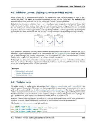
![scikit-learn user guide, Release 0.16.0
>>> np.random.seed(0)
>>> iris = load_iris()
>>> X, y = iris.data, iris.target
>>> indices = np.arange(y.shape[0])
>>> np.random.shuffle(indices)
>>> X, y = X[indices], y[indices]
>>> train_scores, valid_scores = validation_curve(Ridge(), X, y, "alpha",
... np.logspace(-7, 3, 3))
>>> train_scores
array([[ 0.94..., 0.92..., 0.92...],
[ 0.94..., 0.92..., 0.92...],
[ 0.47..., 0.45..., 0.42...]])
>>> valid_scores
array([[ 0.90..., 0.92..., 0.94...],
[ 0.90..., 0.92..., 0.94...],
[ 0.44..., 0.39..., 0.45...]])
If the training score and the validation score are both low, the estimator will be underfitting. If the training score is
high and the validation score is low, the estimator is overfitting and otherwise it is working very well. A low training
score and a high validation score is usually not possible. All three cases can be found in the plot below where we vary
the parameter 𝛾 of an SVM on the digits dataset.
6.5.2 Learning curve
A learning curve shows the validation and training score of an estimator for varying numbers of training samples. It
is a tool to find out how much we benefit from adding more training data and whether the estimator suffers more from
a variance error or a bias error. If both the validation score and the training score converge to a value that is too low
with increasing size of the training set, we will not benefit much from more training data. In the following plot you
can see an example: naive Bayes roughly converges to a low score.
We will probably have to use an estimator or a parametrization of the current estimator that can learn more complex
concepts (i.e. has a lower bias). If the training score is much greater than the validation score for the maximum number
of training samples, adding more training samples will most likely increase generalization. In the following plot you
can see that the SVM could benefit from more training examples.
We can use the function learning_curve to generate the values that are required to plot such a learning curve
(number of samples that have been used, the average scores on the training sets and the average scores on the validation
260 Chapter 6. Model selection and evaluation](https://image.slidesharecdn.com/scikit-learn0-150409112902-conversion-gate01/85/Scikit-learn-0-16-0-user-guide-270-320.jpg)

![scikit-learn user guide, Release 0.16.0
sets):
>>> from sklearn.learning_curve import learning_curve
>>> from sklearn.svm import SVC
>>> train_sizes, train_scores, valid_scores = learning_curve(
... SVC(kernel='linear'), X, y, train_sizes=[50, 80, 110], cv=5)
>>> train_sizes
array([ 50, 80, 110])
>>> train_scores
array([[ 0.98..., 0.98 , 0.98..., 0.98..., 0.98...],
[ 0.98..., 1. , 0.98..., 0.98..., 0.98...],
[ 0.98..., 1. , 0.98..., 0.98..., 0.99...]])
>>> valid_scores
array([[ 1. , 0.93..., 1. , 1. , 0.96...],
[ 1. , 0.96..., 1. , 1. , 0.96...],
[ 1. , 0.96..., 1. , 1. , 0.96...]])
262 Chapter 6. Model selection and evaluation](https://image.slidesharecdn.com/scikit-learn0-150409112902-conversion-gate01/85/Scikit-learn-0-16-0-user-guide-272-320.jpg)
![CHAPTER
SEVEN
DATASET TRANSFORMATIONS
scikit-learn provides a library of transformers, which may clean (see Preprocessing data), reduce (see Unsupervised
dimensionality reduction), expand (see Kernel Approximation) or generate (see Feature extraction) feature representa-
tions.
Like other estimators, these are represented by classes with fit method, which learns model parameters (e.g. mean
and standard deviation for normalization) from a training set, and a transform method which applies this transfor-
mation model to unseen data. fit_transform may be more convenient and efficient for modelling and transform-
ing the training data simultaneously.
Combining such transformers, either in parallel or series is covered in Pipeline and FeatureUnion: combining es-
timators. Pairwise metrics, Affinities and Kernels covers transforming feature spaces into affinity matrices, while
Transforming the prediction target (y) considers transformations of the target space (e.g. categorical labels) for use in
scikit-learn.
7.1 Pipeline and FeatureUnion: combining estimators
7.1.1 Pipeline: chaining estimators
Pipeline can be used to chain multiple estimators into one. This is useful as there is often a fixed sequence of
steps in processing the data, for example feature selection, normalization and classification. Pipeline serves two
purposes here:
Convenience: You only have to call fit and predict once on your data to fit a whole sequence of
estimators.
Joint parameter selection: You can grid search over parameters of all estimators in the pipeline at once.
All estimators in a pipeline, except the last one, must be transformers (i.e. must have a transform method). The
last estimator may be any type (transformer, classifier, etc.).
Usage
The Pipeline is build using a list of (key, value) pairs, where the key a string containing the name you want
to give this step and value is an estimator object:
>>> from sklearn.pipeline import Pipeline
>>> from sklearn.svm import SVC
>>> from sklearn.decomposition import PCA
>>> estimators = [('reduce_dim', PCA()), ('svm', SVC())]
>>> clf = Pipeline(estimators)
>>> clf
Pipeline(steps=[('reduce_dim', PCA(copy=True, n_components=None,
263](https://image.slidesharecdn.com/scikit-learn0-150409112902-conversion-gate01/85/Scikit-learn-0-16-0-user-guide-273-320.jpg)
![scikit-learn user guide, Release 0.16.0
whiten=False)), ('svm', SVC(C=1.0, cache_size=200, class_weight=None,
coef0=0.0, degree=3, gamma=0.0, kernel='rbf', max_iter=-1,
probability=False, random_state=None, shrinking=True, tol=0.001,
verbose=False))])
The utility function make_pipeline is a shorthand for constructing pipelines; it takes a variable number of estima-
tors and returns a pipeline, filling in the names automatically:
>>> from sklearn.pipeline import make_pipeline
>>> from sklearn.naive_bayes import MultinomialNB
>>> from sklearn.preprocessing import Binarizer
>>> make_pipeline(Binarizer(), MultinomialNB())
Pipeline(steps=[('binarizer', Binarizer(copy=True, threshold=0.0)),
('multinomialnb', MultinomialNB(alpha=1.0,
class_prior=None,
fit_prior=True))])
The estimators of a pipeline are stored as a list in the steps attribute:
>>> clf.steps[0]
('reduce_dim', PCA(copy=True, n_components=None, whiten=False))
and as a dict in named_steps:
>>> clf.named_steps['reduce_dim']
PCA(copy=True, n_components=None, whiten=False)
Parameters of the estimators in the pipeline can be accessed using the <estimator>__<parameter> syntax:
>>> clf.set_params(svm__C=10)
Pipeline(steps=[('reduce_dim', PCA(copy=True, n_components=None,
whiten=False)), ('svm', SVC(C=10, cache_size=200, class_weight=None,
coef0=0.0, degree=3, gamma=0.0, kernel='rbf', max_iter=-1,
probability=False, random_state=None, shrinking=True, tol=0.001,
verbose=False))])
This is particularly important for doing grid searches:
>>> from sklearn.grid_search import GridSearchCV
>>> params = dict(reduce_dim__n_components=[2, 5, 10],
... svm__C=[0.1, 10, 100])
>>> grid_search = GridSearchCV(clf, param_grid=params)
Examples:
• Pipeline Anova SVM
• Sample pipeline for text feature extraction and evaluation
• Pipelining: chaining a PCA and a logistic regression
• Explicit feature map approximation for RBF kernels
• SVM-Anova: SVM with univariate feature selection
See also:
• Grid Search: Searching for estimator parameters
264 Chapter 7. Dataset transformations](https://image.slidesharecdn.com/scikit-learn0-150409112902-conversion-gate01/85/Scikit-learn-0-16-0-user-guide-274-320.jpg)
![scikit-learn user guide, Release 0.16.0
Notes
Calling fit on the pipeline is the same as calling fit on each estimator in turn, transform the input and pass it
on to the next step. The pipeline has all the methods that the last estimator in the pipeline has, i.e. if the last estimator
is a classifier, the Pipeline can be used as a classifier. If the last estimator is a transformer, again, so is the pipeline.
7.1.2 FeatureUnion: composite feature spaces
FeatureUnion combines several transformer objects into a new transformer that combines their output. A
FeatureUnion takes a list of transformer objects. During fitting, each of these is fit to the data independently.
For transforming data, the transformers are applied in parallel, and the sample vectors they output are concatenated
end-to-end into larger vectors.
FeatureUnion serves the same purposes as Pipeline - convenience and joint parameter estimation and valida-
tion.
FeatureUnion and Pipeline can be combined to create complex models.
(A FeatureUnion has no way of checking whether two transformers might produce identical features. It only
produces a union when the feature sets are disjoint, and making sure they are is the caller’s responsibility.)
Usage
A FeatureUnion is built using a list of (key, value) pairs, where the key is the name you want to give to a
given transformation (an arbitrary string; it only serves as an identifier) and value is an estimator object:
>>> from sklearn.pipeline import FeatureUnion
>>> from sklearn.decomposition import PCA
>>> from sklearn.decomposition import KernelPCA
>>> estimators = [('linear_pca', PCA()), ('kernel_pca', KernelPCA())]
>>> combined = FeatureUnion(estimators)
>>> combined
FeatureUnion(n_jobs=1, transformer_list=[('linear_pca', PCA(copy=True,
n_components=None, whiten=False)), ('kernel_pca', KernelPCA(alpha=1.0,
coef0=1, degree=3, eigen_solver='auto', fit_inverse_transform=False,
gamma=None, kernel='linear', kernel_params=None, max_iter=None,
n_components=None, remove_zero_eig=False, tol=0))],
transformer_weights=None)
Like pipelines, feature unions have a shorthand constructor called make_union that does require manual naming of
the components.
Examples:
• Concatenating multiple feature extraction methods
• Feature Union with Heterogeneous Data Sources
7.2 Feature extraction
The sklearn.feature_extraction module can be used to extract features in a format supported by machine
learning algorithms from datasets consisting of formats such as text and image.
Note: Feature extraction is very different from Feature selection: the former consists in transforming arbitrary data,
7.2. Feature extraction 265](https://image.slidesharecdn.com/scikit-learn0-150409112902-conversion-gate01/85/Scikit-learn-0-16-0-user-guide-275-320.jpg)
![scikit-learn user guide, Release 0.16.0
such as text or images, into numerical features usable for machine learning. The latter is a machine learning technique
applied on these features.
7.2.1 Loading features from dicts
The class DictVectorizer can be used to convert feature arrays represented as lists of standard Python dict
objects to the NumPy/SciPy representation used by scikit-learn estimators.
While not particularly fast to process, Python’s dict has the advantages of being convenient to use, being sparse
(absent features need not be stored) and storing feature names in addition to values.
DictVectorizer implements what is called one-of-K or “one-hot” coding for categorical (aka nominal, discrete)
features. Categorical features are “attribute-value” pairs where the value is restricted to a list of discrete of possibilities
without ordering (e.g. topic identifiers, types of objects, tags, names...).
In the following, “city” is a categorical attribute while “temperature” is a traditional numerical feature:
>>> measurements = [
... {'city': 'Dubai', 'temperature': 33.},
... {'city': 'London', 'temperature': 12.},
... {'city': 'San Fransisco', 'temperature': 18.},
... ]
>>> from sklearn.feature_extraction import DictVectorizer
>>> vec = DictVectorizer()
>>> vec.fit_transform(measurements).toarray()
array([[ 1., 0., 0., 33.],
[ 0., 1., 0., 12.],
[ 0., 0., 1., 18.]])
>>> vec.get_feature_names()
['city=Dubai', 'city=London', 'city=San Fransisco', 'temperature']
DictVectorizer is also a useful representation transformation for training sequence classifiers in Natural Lan-
guage Processing models that typically work by extracting feature windows around a particular word of interest.
For example, suppose that we have a first algorithm that extracts Part of Speech (PoS) tags that we want to use as
complementary tags for training a sequence classifier (e.g. a chunker). The following dict could be such a window of
features extracted around the word ‘sat’ in the sentence ‘The cat sat on the mat.’:
>>> pos_window = [
... {
... 'word-2': 'the',
... 'pos-2': 'DT',
... 'word-1': 'cat',
... 'pos-1': 'NN',
... 'word+1': 'on',
... 'pos+1': 'PP',
... },
... # in a real application one would extract many such dictionaries
... ]
This description can be vectorized into a sparse two-dimensional matrix suitable for feeding into a classifier (maybe
after being piped into a text.TfidfTransformer for normalization):
>>> vec = DictVectorizer()
>>> pos_vectorized = vec.fit_transform(pos_window)
266 Chapter 7. Dataset transformations](https://image.slidesharecdn.com/scikit-learn0-150409112902-conversion-gate01/85/Scikit-learn-0-16-0-user-guide-276-320.jpg)
![scikit-learn user guide, Release 0.16.0
>>> pos_vectorized
<1x6 sparse matrix of type '<... 'numpy.float64'>'
with 6 stored elements in Compressed Sparse ... format>
>>> pos_vectorized.toarray()
array([[ 1., 1., 1., 1., 1., 1.]])
>>> vec.get_feature_names()
['pos+1=PP', 'pos-1=NN', 'pos-2=DT', 'word+1=on', 'word-1=cat', 'word-2=the']
As you can imagine, if one extracts such a context around each individual word of a corpus of documents the resulting
matrix will be very wide (many one-hot-features) with most of them being valued to zero most of the time. So as to
make the resulting data structure able to fit in memory the DictVectorizer class uses a scipy.sparse matrix
by default instead of a numpy.ndarray.
7.2.2 Feature hashing
The class FeatureHasher is a high-speed, low-memory vectorizer that uses a technique known as feature hashing,
or the “hashing trick”. Instead of building a hash table of the features encountered in training, as the vectorizers
do, instances of FeatureHasher apply a hash function to the features to determine their column index in sample
matrices directly. The result is increased speed and reduced memory usage, at the expense of inspectability; the hasher
does not remember what the input features looked like and has no inverse_transform method.
Since the hash function might cause collisions between (unrelated) features, a signed hash function is used and the
sign of the hash value determines the sign of the value stored in the output matrix for a feature. This way, collisions
are likely to cancel out rather than accumulate error, and the expected mean of any output feature’s value is zero.
If non_negative=True is passed to the constructor, the absolute value is taken. This undoes some of the collision
handling, but allows the output to be passed to estimators like sklearn.naive_bayes.MultinomialNB or
sklearn.feature_selection.chi2 feature selectors that expect non-negative inputs.
FeatureHasher accepts either mappings (like Python’s dict and its variants in the collections module),
(feature, value) pairs, or strings, depending on the constructor parameter input_type. Mapping are treated
as lists of (feature, value) pairs, while single strings have an implicit value of 1, so [’feat1’, ’feat2’,
’feat3’] is interpreted as [(’feat1’, 1), (’feat2’, 1), (’feat3’, 1)]. If a single feature occurs
multiple times in a sample, the associated values will be summed (so (’feat’, 2) and (’feat’, 3.5) become
(’feat’, 5.5)). The output from FeatureHasher is always a scipy.sparse matrix in the CSR format.
Feature hashing can be employed in document classification, but unlike text.CountVectorizer,
FeatureHasher does not do word splitting or any other preprocessing except Unicode-to-UTF-8 encoding; see
Vectorizing a large text corpus with the hashing trick, below, for a combined tokenizer/hasher.
As an example, consider a word-level natural language processing task that needs features extracted from (token,
part_of_speech) pairs. One could use a Python generator function to extract features:
def token_features(token, part_of_speech):
if token.isdigit():
yield "numeric"
else:
yield "token={}".format(token.lower())
yield "token,pos={},{}".format(token, part_of_speech)
if token[0].isupper():
yield "uppercase_initial"
if token.isupper():
yield "all_uppercase"
yield "pos={}".format(part_of_speech)
Then, the raw_X to be fed to FeatureHasher.transform can be constructed using:
7.2. Feature extraction 267](https://image.slidesharecdn.com/scikit-learn0-150409112902-conversion-gate01/85/Scikit-learn-0-16-0-user-guide-277-320.jpg)

![scikit-learn user guide, Release 0.16.0
A corpus of documents can thus be represented by a matrix with one row per document and one column per token
(e.g. word) occurring in the corpus.
We call vectorization the general process of turning a collection of text documents into numerical feature vectors. This
specific strategy (tokenization, counting and normalization) is called the Bag of Words or “Bag of n-grams” represen-
tation. Documents are described by word occurrences while completely ignoring the relative position information of
the words in the document.
Sparsity
As most documents will typically use a very small subset of the words used in the corpus, the resulting matrix will
have many feature values that are zeros (typically more than 99% of them).
For instance a collection of 10,000 short text documents (such as emails) will use a vocabulary with a size in the order
of 100,000 unique words in total while each document will use 100 to 1000 unique words individually.
In order to be able to store such a matrix in memory but also to speed up algebraic operations matrix / vector, imple-
mentations will typically use a sparse representation such as the implementations available in the scipy.sparse
package.
Common Vectorizer usage
CountVectorizer implements both tokenization and occurrence counting in a single class:
>>> from sklearn.feature_extraction.text import CountVectorizer
This model has many parameters, however the default values are quite reasonable (please see the reference documen-
tation for the details):
>>> vectorizer = CountVectorizer(min_df=1)
>>> vectorizer
CountVectorizer(analyzer=...'word', binary=False, decode_error=...'strict',
dtype=<... 'numpy.int64'>, encoding=...'utf-8', input=...'content',
lowercase=True, max_df=1.0, max_features=None, min_df=1,
ngram_range=(1, 1), preprocessor=None, stop_words=None,
strip_accents=None, token_pattern=...'(?u)bww+b',
tokenizer=None, vocabulary=None)
Let’s use it to tokenize and count the word occurrences of a minimalistic corpus of text documents:
>>> corpus = [
... 'This is the first document.',
... 'This is the second second document.',
... 'And the third one.',
... 'Is this the first document?',
... ]
>>> X = vectorizer.fit_transform(corpus)
>>> X
<4x9 sparse matrix of type '<... 'numpy.int64'>'
with 19 stored elements in Compressed Sparse ... format>
The default configuration tokenizes the string by extracting words of at least 2 letters. The specific function that does
this step can be requested explicitly:
>>> analyze = vectorizer.build_analyzer()
>>> analyze("This is a text document to analyze.") == (
... ['this', 'is', 'text', 'document', 'to', 'analyze'])
True
7.2. Feature extraction 269](https://image.slidesharecdn.com/scikit-learn0-150409112902-conversion-gate01/85/Scikit-learn-0-16-0-user-guide-279-320.jpg)
![scikit-learn user guide, Release 0.16.0
Each term found by the analyzer during the fit is assigned a unique integer index corresponding to a column in the
resulting matrix. This interpretation of the columns can be retrieved as follows:
>>> vectorizer.get_feature_names() == (
... ['and', 'document', 'first', 'is', 'one',
... 'second', 'the', 'third', 'this'])
True
>>> X.toarray()
array([[0, 1, 1, 1, 0, 0, 1, 0, 1],
[0, 1, 0, 1, 0, 2, 1, 0, 1],
[1, 0, 0, 0, 1, 0, 1, 1, 0],
[0, 1, 1, 1, 0, 0, 1, 0, 1]]...)
The converse mapping from feature name to column index is stored in the vocabulary_ attribute of the vectorizer:
>>> vectorizer.vocabulary_.get('document')
1
Hence words that were not seen in the training corpus will be completely ignored in future calls to the transform
method:
>>> vectorizer.transform(['Something completely new.']).toarray()
...
array([[0, 0, 0, 0, 0, 0, 0, 0, 0]]...)
Note that in the previous corpus, the first and the last documents have exactly the same words hence are encoded in
equal vectors. In particular we lose the information that the last document is an interrogative form. To preserve some
of the local ordering information we can extract 2-grams of words in addition to the 1-grams (individual words):
>>> bigram_vectorizer = CountVectorizer(ngram_range=(1, 2),
... token_pattern=r'bw+b', min_df=1)
>>> analyze = bigram_vectorizer.build_analyzer()
>>> analyze('Bi-grams are cool!') == (
... ['bi', 'grams', 'are', 'cool', 'bi grams', 'grams are', 'are cool'])
True
The vocabulary extracted by this vectorizer is hence much bigger and can now resolve ambiguities encoded in local
positioning patterns:
>>> X_2 = bigram_vectorizer.fit_transform(corpus).toarray()
>>> X_2
...
array([[0, 0, 1, 1, 1, 1, 1, 0, 0, 0, 0, 0, 1, 1, 0, 0, 0, 0, 1, 1, 0],
[0, 0, 1, 0, 0, 1, 1, 0, 0, 2, 1, 1, 1, 0, 1, 0, 0, 0, 1, 1, 0],
[1, 1, 0, 0, 0, 0, 0, 0, 1, 0, 0, 0, 1, 0, 0, 1, 1, 1, 0, 0, 0],
[0, 0, 1, 1, 1, 1, 0, 1, 0, 0, 0, 0, 1, 1, 0, 0, 0, 0, 1, 0, 1]]...)
In particular the interrogative form “Is this” is only present in the last document:
>>> feature_index = bigram_vectorizer.vocabulary_.get('is this')
>>> X_2[:, feature_index]
array([0, 0, 0, 1]...)
Tf–idf term weighting
In a large text corpus, some words will be very present (e.g. “the”, “a”, “is” in English) hence carrying very little
meaningful information about the actual contents of the document. If we were to feed the direct count data directly to
a classifier those very frequent terms would shadow the frequencies of rarer yet more interesting terms.
270 Chapter 7. Dataset transformations](https://image.slidesharecdn.com/scikit-learn0-150409112902-conversion-gate01/85/Scikit-learn-0-16-0-user-guide-280-320.jpg)
![scikit-learn user guide, Release 0.16.0
In order to re-weight the count features into floating point values suitable for usage by a classifier it is very common
to use the tf–idf transform.
Tf means term-frequency while tf–idf means term-frequency times inverse document-frequency. This is a originally
a term weighting scheme developed for information retrieval (as a ranking function for search engines results), that
has also found good use in document classification and clustering.
This normalization is implemented by the text.TfidfTransformer class:
>>> from sklearn.feature_extraction.text import TfidfTransformer
>>> transformer = TfidfTransformer()
>>> transformer
TfidfTransformer(norm=...'l2', smooth_idf=True, sublinear_tf=False,
use_idf=True)
Again please see the reference documentation for the details on all the parameters.
Let’s take an example with the following counts. The first term is present 100% of the time hence not very interesting.
The two other features only in less than 50% of the time hence probably more representative of the content of the
documents:
>>> counts = [[3, 0, 1],
... [2, 0, 0],
... [3, 0, 0],
... [4, 0, 0],
... [3, 2, 0],
... [3, 0, 2]]
...
>>> tfidf = transformer.fit_transform(counts)
>>> tfidf
<6x3 sparse matrix of type '<... 'numpy.float64'>'
with 9 stored elements in Compressed Sparse ... format>
>>> tfidf.toarray()
array([[ 0.85..., 0. ..., 0.52...],
[ 1. ..., 0. ..., 0. ...],
[ 1. ..., 0. ..., 0. ...],
[ 1. ..., 0. ..., 0. ...],
[ 0.55..., 0.83..., 0. ...],
[ 0.63..., 0. ..., 0.77...]])
Each row is normalized to have unit euclidean norm. The weights of each feature computed by the fit method call
are stored in a model attribute:
>>> transformer.idf_
array([ 1. ..., 2.25..., 1.84...])
As tf–idf is very often used for text features, there is also another class called TfidfVectorizer that combines all
the options of CountVectorizer and TfidfTransformer in a single model:
>>> from sklearn.feature_extraction.text import TfidfVectorizer
>>> vectorizer = TfidfVectorizer(min_df=1)
>>> vectorizer.fit_transform(corpus)
...
<4x9 sparse matrix of type '<... 'numpy.float64'>'
with 19 stored elements in Compressed Sparse ... format>
While the tf–idf normalization is often very useful, there might be cases where the binary occurrence markers might
offer better features. This can be achieved by using the binary parameter of CountVectorizer. In particular,
7.2. Feature extraction 271](https://image.slidesharecdn.com/scikit-learn0-150409112902-conversion-gate01/85/Scikit-learn-0-16-0-user-guide-281-320.jpg)
![scikit-learn user guide, Release 0.16.0
some estimators such as Bernoulli Naive Bayes explicitly model discrete boolean random variables. Also, very short
texts are likely to have noisy tf–idf values while the binary occurrence info is more stable.
As usual the best way to adjust the feature extraction parameters is to use a cross-validated grid search, for instance by
pipelining the feature extractor with a classifier:
• Sample pipeline for text feature extraction and evaluation
Decoding text files
Text is made of characters, but files are made of bytes. These bytes represent characters according to some encoding.
To work with text files in Python, their bytes must be decoded to a character set called Unicode. Common encodings
are ASCII, Latin-1 (Western Europe), KOI8-R (Russian) and the universal encodings UTF-8 and UTF-16. Many
others exist.
Note: An encoding can also be called a ‘character set’, but this term is less accurate: several encodings can exist for
a single character set.
The text feature extractors in scikit-learn know how to decode text files, but only if you tell them what encoding the
files are in. The CountVectorizer takes an encoding parameter for this purpose. For modern text files, the
correct encoding is probably UTF-8, which is therefore the default (encoding="utf-8").
If the text you are loading is not actually encoded with UTF-8, however, you will get a UnicodeDecodeError.
The vectorizers can be told to be silent about decoding errors by setting the decode_error parameter to either
"ignore" or "replace". See the documentation for the Python function bytes.decode for more details (type
help(bytes.decode) at the Python prompt).
If you are having trouble decoding text, here are some things to try:
• Find out what the actual encoding of the text is. The file might come with a header or README that tells you
the encoding, or there might be some standard encoding you can assume based on where the text comes from.
• You may be able to find out what kind of encoding it is in general using the UNIX command file. The Python
chardet module comes with a script called chardetect.py that will guess the specific encoding, though
you cannot rely on its guess being correct.
• You could try UTF-8 and disregard the errors. You can decode byte strings with
bytes.decode(errors=’replace’) to replace all decoding errors with a meaningless character,
or set decode_error=’replace’ in the vectorizer. This may damage the usefulness of your features.
• Real text may come from a variety of sources that may have used different encodings, or even be sloppily
decoded in a different encoding than the one it was encoded with. This is common in text retrieved from the
Web. The Python package ftfy can automatically sort out some classes of decoding errors, so you could try
decoding the unknown text as latin-1 and then using ftfy to fix errors.
• If the text is in a mish-mash of encodings that is simply too hard to sort out (which is the case for the 20
Newsgroups dataset), you can fall back on a simple single-byte encoding such as latin-1. Some text may
display incorrectly, but at least the same sequence of bytes will always represent the same feature.
For example, the following snippet uses chardet (not shipped with scikit-learn, must be installed separately) to
figure out the encoding of three texts. It then vectorizes the texts and prints the learned vocabulary. The output is not
shown here.
>>> import chardet
>>> text1 = b"Sei mir gegrxc3xbcxc3x9ft mein Sauerkraut"
>>> text2 = b"holdselig sind deine Gerxfcche"
>>> text3 = b"xffxfeAx00ux00fx00 x00Fx00lx00xfcx00gx00ex00lx00nx00 x00dx00ex00sx00
>>> decoded = [x.decode(chardet.detect(x)['encoding'])
... for x in (text1, text2, text3)]
272 Chapter 7. Dataset transformations](https://image.slidesharecdn.com/scikit-learn0-150409112902-conversion-gate01/85/Scikit-learn-0-16-0-user-guide-282-320.jpg)
![scikit-learn user guide, Release 0.16.0
>>> v = CountVectorizer().fit(decoded).vocabulary_
>>> for term in v: print(v)
(Depending on the version of chardet, it might get the first one wrong.)
For an introduction to Unicode and character encodings in general, see Joel Spolsky’s Absolute Minimum Every
Software Developer Must Know About Unicode.
Applications and examples
The bag of words representation is quite simplistic but surprisingly useful in practice.
In particular in a supervised setting it can be successfully combined with fast and scalable linear models to train
document classifiers, for instance:
• Classification of text documents using sparse features
In an unsupervised setting it can be used to group similar documents together by applying clustering algorithms such
as K-means:
• Clustering text documents using k-means
Finally it is possible to discover the main topics of a corpus by relaxing the hard assignment constraint of clustering,
for instance by using Non-negative matrix factorization (NMF or NNMF):
• Topics extraction with Non-Negative Matrix Factorization
Limitations of the Bag of Words representation
A collection of unigrams (what bag of words is) cannot capture phrases and multi-word expressions, effectively disre-
garding any word order dependence. Additionally, the bag of words model doesn’t account for potential misspellings
or word derivations.
N-grams to the rescue! Instead of building a simple collection of unigrams (n=1), one might prefer a collection of
bigrams (n=2), where occurrences of pairs of consecutive words are counted.
One might alternatively consider a collection of character n-grams, a representation resilient against misspellings and
derivations.
For example, let’s say we’re dealing with a corpus of two documents: [’words’, ’wprds’]. The second docu-
ment contains a misspelling of the word ‘words’. A simple bag of words representation would consider these two as
very distinct documents, differing in both of the two possible features. A character 2-gram representation, however,
would find the documents matching in 4 out of 8 features, which may help the preferred classifier decide better:
>>> ngram_vectorizer = CountVectorizer(analyzer='char_wb', ngram_range=(2, 2), min_df=1)
>>> counts = ngram_vectorizer.fit_transform(['words', 'wprds'])
>>> ngram_vectorizer.get_feature_names() == (
... [' w', 'ds', 'or', 'pr', 'rd', 's ', 'wo', 'wp'])
True
>>> counts.toarray().astype(int)
array([[1, 1, 1, 0, 1, 1, 1, 0],
[1, 1, 0, 1, 1, 1, 0, 1]])
In the above example, ’char_wb analyzer is used, which creates n-grams only from characters inside word bound-
aries (padded with space on each side). The ’char’ analyzer, alternatively, creates n-grams that span across words:
>>> ngram_vectorizer = CountVectorizer(analyzer='char_wb', ngram_range=(5, 5), min_df=1)
>>> ngram_vectorizer.fit_transform(['jumpy fox'])
...
7.2. Feature extraction 273](https://image.slidesharecdn.com/scikit-learn0-150409112902-conversion-gate01/85/Scikit-learn-0-16-0-user-guide-283-320.jpg)
![scikit-learn user guide, Release 0.16.0
<1x4 sparse matrix of type '<... 'numpy.int64'>'
with 4 stored elements in Compressed Sparse ... format>
>>> ngram_vectorizer.get_feature_names() == (
... [' fox ', ' jump', 'jumpy', 'umpy '])
True
>>> ngram_vectorizer = CountVectorizer(analyzer='char', ngram_range=(5, 5), min_df=1)
>>> ngram_vectorizer.fit_transform(['jumpy fox'])
...
<1x5 sparse matrix of type '<... 'numpy.int64'>'
with 5 stored elements in Compressed Sparse ... format>
>>> ngram_vectorizer.get_feature_names() == (
... ['jumpy', 'mpy f', 'py fo', 'umpy ', 'y fox'])
True
The word boundaries-aware variant char_wb is especially interesting for languages that use white-spaces for word
separation as it generates significantly less noisy features than the raw char variant in that case. For such languages
it can increase both the predictive accuracy and convergence speed of classifiers trained using such features while
retaining the robustness with regards to misspellings and word derivations.
While some local positioning information can be preserved by extracting n-grams instead of individual words, bag of
words and bag of n-grams destroy most of the inner structure of the document and hence most of the meaning carried
by that internal structure.
In order to address the wider task of Natural Language Understanding, the local structure of sentences and paragraphs
should thus be taken into account. Many such models will thus be casted as “Structured output” problems which are
currently outside of the scope of scikit-learn.
Vectorizing a large text corpus with the hashing trick
The above vectorization scheme is simple but the fact that it holds an in- memory mapping from the string tokens
to the integer feature indices (the vocabulary_ attribute) causes several problems when dealing with large
datasets:
• the larger the corpus, the larger the vocabulary will grow and hence the memory use too,
• fitting requires the allocation of intermediate data structures of size proportional to that of the original dataset.
• building the word-mapping requires a full pass over the dataset hence it is not possible to fit text classifiers in a
strictly online manner.
• pickling and un-pickling vectorizers with a large vocabulary_ can be very slow (typically much slower than
pickling / un-pickling flat data structures such as a NumPy array of the same size),
• it is not easily possible to split the vectorization work into concurrent sub tasks as the vocabulary_ attribute
would have to be a shared state with a fine grained synchronization barrier: the mapping from token string
to feature index is dependent on ordering of the first occurrence of each token hence would have to be shared,
potentially harming the concurrent workers’ performance to the point of making them slower than the sequential
variant.
It is possible to overcome those limitations by combining the “hashing trick” (Feature hashing) implemented by the
sklearn.feature_extraction.FeatureHasher class and the text preprocessing and tokenization features
of the CountVectorizer.
This combination is implementing in HashingVectorizer, a transformer class that is mostly API compatible with
CountVectorizer. HashingVectorizer is stateless, meaning that you don’t have to call fit on it:
>>> from sklearn.feature_extraction.text import HashingVectorizer
>>> hv = HashingVectorizer(n_features=10)
274 Chapter 7. Dataset transformations](https://image.slidesharecdn.com/scikit-learn0-150409112902-conversion-gate01/85/Scikit-learn-0-16-0-user-guide-284-320.jpg)

![scikit-learn user guide, Release 0.16.0
>>> vectorizer.build_analyzer()(u"Some... punctuation!") == (
... ['some...', 'punctuation!'])
True
In particular we name:
• preprocessor: a callable that takes an entire document as input (as a single string), and returns a possibly
transformed version of the document, still as an entire string. This can be used to remove HTML tags, lowercase
the entire document, etc.
• tokenizer: a callable that takes the output from the preprocessor and splits it into tokens, then returns a list
of these.
• analyzer: a callable that replaces the preprocessor and tokenizer. The default analyzers all call the prepro-
cessor and tokenizer, but custom analyzers will skip this. N-gram extraction and stop word filtering take place
at the analyzer level, so a custom analyzer may have to reproduce these steps.
(Lucene users might recognize these names, but be aware that scikit-learn concepts may not map one-to-one onto
Lucene concepts.)
To make the preprocessor, tokenizer and analyzers aware of the model parameters it is possible to derive from the
class and override the build_preprocessor, build_tokenizer‘ and build_analyzer factory methods
instead of passing custom functions.
Some tips and tricks:
• If documents are pre-tokenized by an external package, then store them in files (or strings) with the tokens
separated by whitespace and pass analyzer=str.split
• Fancy token-level analysis such as stemming, lemmatizing, compound splitting, filtering based on part-of-
speech, etc. are not included in the scikit-learn codebase, but can be added by customizing either the tokenizer
or the analyzer. Here’s a CountVectorizer with a tokenizer and lemmatizer using NLTK:
>>> from nltk import word_tokenize
>>> from nltk.stem import WordNetLemmatizer
>>> class LemmaTokenizer(object):
... def __init__(self):
... self.wnl = WordNetLemmatizer()
... def __call__(self, doc):
... return [self.wnl.lemmatize(t) for t in word_tokenize(doc)]
...
>>> vect = CountVectorizer(tokenizer=LemmaTokenizer())
(Note that this will not filter out punctuation.)
Customizing the vectorizer can also be useful when handling Asian languages that do not use an explicit word separator
such as whitespace.
7.2.4 Image feature extraction
Patch extraction
The extract_patches_2d function extracts patches from an image stored as a two-dimensional array, or
three-dimensional with color information along the third axis. For rebuilding an image from all its patches, use
reconstruct_from_patches_2d. For example let use generate a 4x4 pixel picture with 3 color channels (e.g.
in RGB format):
276 Chapter 7. Dataset transformations](https://image.slidesharecdn.com/scikit-learn0-150409112902-conversion-gate01/85/Scikit-learn-0-16-0-user-guide-286-320.jpg)
![scikit-learn user guide, Release 0.16.0
>>> import numpy as np
>>> from sklearn.feature_extraction import image
>>> one_image = np.arange(4 * 4 * 3).reshape((4, 4, 3))
>>> one_image[:, :, 0] # R channel of a fake RGB picture
array([[ 0, 3, 6, 9],
[12, 15, 18, 21],
[24, 27, 30, 33],
[36, 39, 42, 45]])
>>> patches = image.extract_patches_2d(one_image, (2, 2), max_patches=2,
... random_state=0)
>>> patches.shape
(2, 2, 2, 3)
>>> patches[:, :, :, 0]
array([[[ 0, 3],
[12, 15]],
[[15, 18],
[27, 30]]])
>>> patches = image.extract_patches_2d(one_image, (2, 2))
>>> patches.shape
(9, 2, 2, 3)
>>> patches[4, :, :, 0]
array([[15, 18],
[27, 30]])
Let us now try to reconstruct the original image from the patches by averaging on overlapping areas:
>>> reconstructed = image.reconstruct_from_patches_2d(patches, (4, 4, 3))
>>> np.testing.assert_array_equal(one_image, reconstructed)
The PatchExtractor class works in the same way as extract_patches_2d, only it supports multiple images
as input. It is implemented as an estimator, so it can be used in pipelines. See:
>>> five_images = np.arange(5 * 4 * 4 * 3).reshape(5, 4, 4, 3)
>>> patches = image.PatchExtractor((2, 2)).transform(five_images)
>>> patches.shape
(45, 2, 2, 3)
Connectivity graph of an image
Several estimators in the scikit-learn can use connectivity information between features or samples. For instance Ward
clustering (Hierarchical clustering) can cluster together only neighboring pixels of an image, thus forming contiguous
patches:
For this purpose, the estimators use a ‘connectivity’ matrix, giving which samples are connected.
The function img_to_graph returns such a matrix from a 2D or 3D image. Similarly, grid_to_graph build a
connectivity matrix for images given the shape of these image.
These matrices can be used to impose connectivity in estimators that use connectivity information, such as Ward
clustering (Hierarchical clustering), but also to build precomputed kernels, or similarity matrices.
Note: Examples
• A demo of structured Ward hierarchical clustering on Lena image
• Spectral clustering for image segmentation
7.2. Feature extraction 277](https://image.slidesharecdn.com/scikit-learn0-150409112902-conversion-gate01/85/Scikit-learn-0-16-0-user-guide-287-320.jpg)
![scikit-learn user guide, Release 0.16.0
• Feature agglomeration vs. univariate selection
7.3 Preprocessing data
The sklearn.preprocessing package provides several common utility functions and transformer classes to
change raw feature vectors into a representation that is more suitable for the downstream estimators.
7.3.1 Standardization, or mean removal and variance scaling
Standardization of datasets is a common requirement for many machine learning estimators implemented in the
scikit: they might behave badly if the individual feature do not more or less look like standard normally distributed
data: Gaussian with zero mean and unit variance.
In practice we often ignore the shape of the distribution and just transform the data to center it by removing the mean
value of each feature, then scale it by dividing non-constant features by their standard deviation.
For instance, many elements used in the objective function of a learning algorithm (such as the RBF kernel of Support
Vector Machines or the l1 and l2 regularizers of linear models) assume that all features are centered around zero and
have variance in the same order. If a feature has a variance that is orders of magnitude larger that others, it might
dominate the objective function and make the estimator unable to learn from other features correctly as expected.
The function scale provides a quick and easy way to perform this operation on a single array-like dataset:
>>> from sklearn import preprocessing
>>> import numpy as np
>>> X = np.array([[ 1., -1., 2.],
... [ 2., 0., 0.],
... [ 0., 1., -1.]])
>>> X_scaled = preprocessing.scale(X)
>>> X_scaled
array([[ 0. ..., -1.22..., 1.33...],
[ 1.22..., 0. ..., -0.26...],
[-1.22..., 1.22..., -1.06...]])
Scaled data has zero mean and unit variance:
>>> X_scaled.mean(axis=0)
array([ 0., 0., 0.])
278 Chapter 7. Dataset transformations](https://image.slidesharecdn.com/scikit-learn0-150409112902-conversion-gate01/85/Scikit-learn-0-16-0-user-guide-288-320.jpg)
![scikit-learn user guide, Release 0.16.0
>>> X_scaled.std(axis=0)
array([ 1., 1., 1.])
The preprocessing module further provides a utility class StandardScaler that implements the
Transformer API to compute the mean and standard deviation on a training set so as to be able to later
reapply the same transformation on the testing set. This class is hence suitable for use in the early steps of a
sklearn.pipeline.Pipeline:
>>> scaler = preprocessing.StandardScaler().fit(X)
>>> scaler
StandardScaler(copy=True, with_mean=True, with_std=True)
>>> scaler.mean_
array([ 1. ..., 0. ..., 0.33...])
>>> scaler.std_
array([ 0.81..., 0.81..., 1.24...])
>>> scaler.transform(X)
array([[ 0. ..., -1.22..., 1.33...],
[ 1.22..., 0. ..., -0.26...],
[-1.22..., 1.22..., -1.06...]])
The scaler instance can then be used on new data to transform it the same way it did on the training set:
>>> scaler.transform([[-1., 1., 0.]])
array([[-2.44..., 1.22..., -0.26...]])
It is possible to disable either centering or scaling by either passing with_mean=False or with_std=False to
the constructor of StandardScaler.
Scaling features to a range
An alternative standardization is scaling features to lie between a given minimum and maximum value, often between
zero and one. This can be achieved using MinMaxScaler.
The motivation to use this scaling include robustness to very small standard deviations of features and preserving zero
entries in sparse data.
Here is an example to scale a toy data matrix to the [0, 1] range:
>>> X_train = np.array([[ 1., -1., 2.],
... [ 2., 0., 0.],
... [ 0., 1., -1.]])
...
>>> min_max_scaler = preprocessing.MinMaxScaler()
>>> X_train_minmax = min_max_scaler.fit_transform(X_train)
>>> X_train_minmax
array([[ 0.5 , 0. , 1. ],
[ 1. , 0.5 , 0.33333333],
[ 0. , 1. , 0. ]])
The same instance of the transformer can then be applied to some new test data unseen during the fit call: the same
scaling and shifting operations will be applied to be consistent with the transformation performed on the train data:
>>> X_test = np.array([[ -3., -1., 4.]])
>>> X_test_minmax = min_max_scaler.transform(X_test)
>>> X_test_minmax
array([[-1.5 , 0. , 1.66666667]])
7.3. Preprocessing data 279](https://image.slidesharecdn.com/scikit-learn0-150409112902-conversion-gate01/85/Scikit-learn-0-16-0-user-guide-289-320.jpg)
![scikit-learn user guide, Release 0.16.0
It is possible to introspect the scaler attributes to find about the exact nature of the transformation learned on the
training data:
>>> min_max_scaler.scale_
array([ 0.5 , 0.5 , 0.33...])
>>> min_max_scaler.min_
array([ 0. , 0.5 , 0.33...])
If MinMaxScaler is given an explicit feature_range=(min, max) the full formula is:
X_std = (X - X.min(axis=0)) / (X.max(axis=0) - X.min(axis=0))
X_scaled = X_std / (max - min) + min
References:
Further discussion on the importance of centering and scaling data is available on this FAQ: Should I normal-
ize/standardize/rescale the data?
Scaling vs Whitening
It is sometimes not enough to center and scale the features independently, since a downstream model can further
make some assumption on the linear independence of the features.
To address this issue you can use sklearn.decomposition.PCA or
sklearn.decomposition.RandomizedPCA with whiten=True to further remove the linear
correlation across features.
Sparse input
scale and StandardScaler accept scipy.sparse matrices as input only when with_mean=False is
explicitly passed to the constructor. Otherwise a ValueError will be raised as silently centering would
break the sparsity and would often crash the execution by allocating excessive amounts of memory unintention-
ally.
If the centered data is expected to be small enough, explicitly convert the input to an array using the toarray
method of sparse matrices instead.
For sparse input the data is converted to the Compressed Sparse Rows representation (see
scipy.sparse.csr_matrix). To avoid unnecessary memory copies, it is recommended to choose the
CSR representation upstream.
Scaling target variables in regression
scale and StandardScaler work out-of-the-box with 1d arrays. This is very useful for scaling the target /
response variables used for regression.
Centering kernel matrices
If you have a kernel matrix of a kernel 𝐾 that computes a dot product in a feature space defined by function 𝑝ℎ𝑖, a
KernelCenterer can transform the kernel matrix so that it contains inner products in the feature space defined by
280 Chapter 7. Dataset transformations](https://image.slidesharecdn.com/scikit-learn0-150409112902-conversion-gate01/85/Scikit-learn-0-16-0-user-guide-290-320.jpg)
![scikit-learn user guide, Release 0.16.0
𝑝ℎ𝑖 followed by removal of the mean in that space.
7.3.2 Normalization
Normalization is the process of scaling individual samples to have unit norm. This process can be useful if you plan
to use a quadratic form such as the dot-product or any other kernel to quantify the similarity of any pair of samples.
This assumption is the base of the Vector Space Model often used in text classification and clustering contexts.
The function normalize provides a quick and easy way to perform this operation on a single array-like dataset,
either using the l1 or l2 norms:
>>> X = [[ 1., -1., 2.],
... [ 2., 0., 0.],
... [ 0., 1., -1.]]
>>> X_normalized = preprocessing.normalize(X, norm='l2')
>>> X_normalized
array([[ 0.40..., -0.40..., 0.81...],
[ 1. ..., 0. ..., 0. ...],
[ 0. ..., 0.70..., -0.70...]])
The preprocessing module further provides a utility class Normalizer that implements the same operation
using the Transformer API (even though the fit method is useless in this case: the class is stateless as this
operation treats samples independently).
This class is hence suitable for use in the early steps of a sklearn.pipeline.Pipeline:
>>> normalizer = preprocessing.Normalizer().fit(X) # fit does nothing
>>> normalizer
Normalizer(copy=True, norm='l2')
The normalizer instance can then be used on sample vectors as any transformer:
>>> normalizer.transform(X)
array([[ 0.40..., -0.40..., 0.81...],
[ 1. ..., 0. ..., 0. ...],
[ 0. ..., 0.70..., -0.70...]])
>>> normalizer.transform([[-1., 1., 0.]])
array([[-0.70..., 0.70..., 0. ...]])
Sparse input
normalize and Normalizer accept both dense array-like and sparse matrices from scipy.sparse as
input.
For sparse input the data is converted to the Compressed Sparse Rows representation (see
scipy.sparse.csr_matrix) before being fed to efficient Cython routines. To avoid unnecessary memory
copies, it is recommended to choose the CSR representation upstream.
7.3. Preprocessing data 281](https://image.slidesharecdn.com/scikit-learn0-150409112902-conversion-gate01/85/Scikit-learn-0-16-0-user-guide-291-320.jpg)
![scikit-learn user guide, Release 0.16.0
7.3.3 Binarization
Feature binarization
Feature binarization is the process of thresholding numerical features to get boolean values. This can be useful for
downstream probabilistic estimators that make assumption that the input data is distributed according to a multi-variate
Bernoulli distribution. For instance, this is the case for the sklearn.neural_network.BernoulliRBM.
It is also common among the text processing community to use binary feature values (probably to simplify the proba-
bilistic reasoning) even if normalized counts (a.k.a. term frequencies) or TF-IDF valued features often perform slightly
better in practice.
As for the Normalizer, the utility class Binarizer is meant to be used in the early stages of
sklearn.pipeline.Pipeline. The fit method does nothing as each sample is treated independently of
others:
>>> X = [[ 1., -1., 2.],
... [ 2., 0., 0.],
... [ 0., 1., -1.]]
>>> binarizer = preprocessing.Binarizer().fit(X) # fit does nothing
>>> binarizer
Binarizer(copy=True, threshold=0.0)
>>> binarizer.transform(X)
array([[ 1., 0., 1.],
[ 1., 0., 0.],
[ 0., 1., 0.]])
It is possible to adjust the threshold of the binarizer:
>>> binarizer = preprocessing.Binarizer(threshold=1.1)
>>> binarizer.transform(X)
array([[ 0., 0., 1.],
[ 1., 0., 0.],
[ 0., 0., 0.]])
As for the StandardScaler and Normalizer classes, the preprocessing module provides a companion function
binarize to be used when the transformer API is not necessary.
Sparse input
binarize and Binarizer accept both dense array-like and sparse matrices from scipy.sparse as input.
For sparse input the data is converted to the Compressed Sparse Rows representation (see
scipy.sparse.csr_matrix). To avoid unnecessary memory copies, it is recommended to choose the
CSR representation upstream.
7.3.4 Encoding categorical features
Often features are not given as continuous values but categorical. For example a person could have fea-
tures ["male", "female"], ["from Europe", "from US", "from Asia"], ["uses Firefox",
"uses Chrome", "uses Safari", "uses Internet Explorer"]. Such features can be efficiently
coded as integers, for instance ["male", "from US", "uses Internet Explorer"] could be expressed
as [0, 1, 3] while ["female", "from Asia", "uses Chrome"] would be [1, 2, 1].
282 Chapter 7. Dataset transformations](https://image.slidesharecdn.com/scikit-learn0-150409112902-conversion-gate01/85/Scikit-learn-0-16-0-user-guide-292-320.jpg)
![scikit-learn user guide, Release 0.16.0
Such integer representation can not be used directly with scikit-learn estimators, as these expect continuous input,
and would interpret the categories as being ordered, which is often not desired (i.e. the set of browsers was ordered
arbitrarily).
One possibility to convert categorical features to features that can be used with scikit-learn estimators is to use a one-
of-K or one-hot encoding, which is implemented in OneHotEncoder. This estimator transforms each categorical
feature with m possible values into m binary features, with only one active.
Continuing the example above:
>>> enc = preprocessing.OneHotEncoder()
>>> enc.fit([[0, 0, 3], [1, 1, 0], [0, 2, 1], [1, 0, 2]])
OneHotEncoder(categorical_features='all', dtype=<... 'float'>,
handle_unknown='error', n_values='auto', sparse=True)
>>> enc.transform([[0, 1, 3]]).toarray()
array([[ 1., 0., 0., 1., 0., 0., 0., 0., 1.]])
By default, how many values each feature can take is inferred automatically from the dataset. It is possible to specify
this explicitly using the parameter n_values. There are two genders, three possible continents and four web browsers
in our dataset. Then we fit the estimator, and transform a data point. In the result, the first two numbers encode the
gender, the next set of three numbers the continent and the last four the web browser.
See Loading features from dicts for categorical features that are represented as a dict, not as integers.
7.3.5 Imputation of missing values
For various reasons, many real world datasets contain missing values, often encoded as blanks, NaNs or other place-
holders. Such datasets however are incompatible with scikit-learn estimators which assume that all values in an array
are numerical, and that all have and hold meaning. A basic strategy to use incomplete datasets is to discard entire rows
and/or columns containing missing values. However, this comes at the price of losing data which may be valuable
(even though incomplete). A better strategy is to impute the missing values, i.e., to infer them from the known part of
the data.
The Imputer class provides basic strategies for imputing missing values, either using the mean, the median or the
most frequent value of the row or column in which the missing values are located. This class also allows for different
missing values encodings.
The following snippet demonstrates how to replace missing values, encoded as np.nan, using the mean value of the
columns (axis 0) that contain the missing values:
>>> import numpy as np
>>> from sklearn.preprocessing import Imputer
>>> imp = Imputer(missing_values='NaN', strategy='mean', axis=0)
>>> imp.fit([[1, 2], [np.nan, 3], [7, 6]])
Imputer(axis=0, copy=True, missing_values='NaN', strategy='mean', verbose=0)
>>> X = [[np.nan, 2], [6, np.nan], [7, 6]]
>>> print(imp.transform(X))
[[ 4. 2. ]
[ 6. 3.666...]
[ 7. 6. ]]
The Imputer class also supports sparse matrices:
>>> import scipy.sparse as sp
>>> X = sp.csc_matrix([[1, 2], [0, 3], [7, 6]])
>>> imp = Imputer(missing_values=0, strategy='mean', axis=0)
>>> imp.fit(X)
Imputer(axis=0, copy=True, missing_values=0, strategy='mean', verbose=0)
>>> X_test = sp.csc_matrix([[0, 2], [6, 0], [7, 6]])
7.3. Preprocessing data 283](https://image.slidesharecdn.com/scikit-learn0-150409112902-conversion-gate01/85/Scikit-learn-0-16-0-user-guide-293-320.jpg)
![scikit-learn user guide, Release 0.16.0
>>> print(imp.transform(X_test))
[[ 4. 2. ]
[ 6. 3.666...]
[ 7. 6. ]]
Note that, here, missing values are encoded by 0 and are thus implicitly stored in the matrix. This format is thus
suitable when there are many more missing values than observed values.
Imputer can be used in a Pipeline as a way to build a composite estimator that supports imputation. See Imputing
missing values before building an estimator
7.4 Unsupervised dimensionality reduction
If your number of features is high, it may be useful to reduce it with an unsupervised step prior to supervised steps.
Many of the Unsupervised learning methods implement a transform method that can be used to reduce the dimen-
sionality. Below we discuss two specific example of this pattern that are heavily used.
Pipelining
The unsupervised data reduction and the supervised estimator can be chained in one step. See Pipeline: chaining
estimators.
7.4.1 PCA: principal component analysis
decomposition.PCA looks for a combination of features that capture well the variance of the original features.
See Decomposing signals in components (matrix factorization problems).
Examples
• Faces recognition example using eigenfaces and SVMs
7.4.2 Random projections
The module: random_projection provides several tools for data reduction by random projections. See the
relevant section of the documentation: Random Projection.
Examples
• The Johnson-Lindenstrauss bound for embedding with random projections
7.4.3 Feature agglomeration
cluster.FeatureAgglomeration applies Hierarchical clustering to group together features that behave sim-
ilarly.
284 Chapter 7. Dataset transformations](https://image.slidesharecdn.com/scikit-learn0-150409112902-conversion-gate01/85/Scikit-learn-0-16-0-user-guide-294-320.jpg)
![scikit-learn user guide, Release 0.16.0
Examples
• Feature agglomeration vs. univariate selection
• Feature agglomeration
Feature scaling
Note that if features have very different scaling or statistical properties,
cluster.FeatureAgglomeration may not be able to capture the links between related features.
Using a preprocessing.StandardScaler can be useful in these settings.
7.5 Random Projection
The sklearn.random_projection module implements a simple and computationally efficient way to reduce
the dimensionality of the data by trading a controlled amount of accuracy (as additional variance) for faster processing
times and smaller model sizes. This module implements two types of unstructured random matrix: Gaussian random
matrix and sparse random matrix.
The dimensions and distribution of random projections matrices are controlled so as to preserve the pairwise distances
between any two samples of the dataset. Thus random projection is a suitable approximation technique for distance
based method.
References:
• Sanjoy Dasgupta. 2000. Experiments with random projection. In Proceedings of the Sixteenth conference
on Uncertainty in artificial intelligence (UAI‘00), Craig Boutilier and Moisés Goldszmidt (Eds.). Morgan
Kaufmann Publishers Inc., San Francisco, CA, USA, 143-151.
• Ella Bingham and Heikki Mannila. 2001. Random projection in dimensionality reduction: applications to
image and text data. In Proceedings of the seventh ACM SIGKDD international conference on Knowledge
discovery and data mining (KDD ‘01). ACM, New York, NY, USA, 245-250.
7.5.1 The Johnson-Lindenstrauss lemma
The main theoretical result behind the efficiency of random projection is the Johnson-Lindenstrauss lemma (quoting
Wikipedia):
In mathematics, the Johnson-Lindenstrauss lemma is a result concerning low-distortion embeddings of
points from high-dimensional into low-dimensional Euclidean space. The lemma states that a small set
of points in a high-dimensional space can be embedded into a space of much lower dimension in such a
way that distances between the points are nearly preserved. The map used for the embedding is at least
Lipschitz, and can even be taken to be an orthogonal projection.
Knowing only the number of samples, the sklearn.random_projection.johnson_lindenstrauss_min_dim
estimates conservatively the minimal size of the random subspace to guarantee a bounded distortion introduced by the
random projection:
>>> from sklearn.random_projection import johnson_lindenstrauss_min_dim
>>> johnson_lindenstrauss_min_dim(n_samples=1e6, eps=0.5)
663
>>> johnson_lindenstrauss_min_dim(n_samples=1e6, eps=[0.5, 0.1, 0.01])
7.5. Random Projection 285](https://image.slidesharecdn.com/scikit-learn0-150409112902-conversion-gate01/85/Scikit-learn-0-16-0-user-guide-295-320.jpg)
![scikit-learn user guide, Release 0.16.0
array([ 663, 11841, 1112658])
>>> johnson_lindenstrauss_min_dim(n_samples=[1e4, 1e5, 1e6], eps=0.1)
array([ 7894, 9868, 11841])
Example:
• See The Johnson-Lindenstrauss bound for embedding with random projections for a theoretical explication
on the Johnson-Lindenstrauss lemma and an empirical validation using sparse random matrices.
References:
• Sanjoy Dasgupta and Anupam Gupta, 1999. An elementary proof of the Johnson-Lindenstrauss Lemma.
7.5.2 Gaussian random projection
The sklearn.random_projection.GaussianRandomProjection reduces the dimensionality by pro-
jecting the original input space on a randomly generated matrix where components are drawn from the following
distribution 𝑁(0, 1
𝑛 𝑐𝑜𝑚𝑝𝑜𝑛𝑒𝑛𝑡𝑠
).
Here a small excerpt which illustrates how to use the Gaussian random projection transformer:
>>> import numpy as np
>>> from sklearn import random_projection
>>> X = np.random.rand(100, 10000)
>>> transformer = random_projection.GaussianRandomProjection()
>>> X_new = transformer.fit_transform(X)
>>> X_new.shape
(100, 3947)
286 Chapter 7. Dataset transformations](https://image.slidesharecdn.com/scikit-learn0-150409112902-conversion-gate01/85/Scikit-learn-0-16-0-user-guide-296-320.jpg)

![scikit-learn user guide, Release 0.16.0
References:
• D. Achlioptas. 2003. Database-friendly random projections: Johnson-Lindenstrauss with binary coins.
Journal of Computer and System Sciences 66 (2003) 671–687
• Ping Li, Trevor J. Hastie, and Kenneth W. Church. 2006. Very sparse random projections. In Proceedings
of the 12th ACM SIGKDD international conference on Knowledge discovery and data mining (KDD ‘06).
ACM, New York, NY, USA, 287-296.
7.6 Kernel Approximation
This submodule contains functions that approximate the feature mappings that correspond to certain kernels, as they
are used for example in support vector machines (see Support Vector Machines). The following feature functions
perform non-linear transformations of the input, which can serve as a basis for linear classification or other algorithms.
The advantage of using approximate explicit feature maps compared to the kernel trick, which makes use of feature
maps implicitly, is that explicit mappings can be better suited for online learning and can significantly reduce the
cost of learning with very large datasets. Standard kernelized SVMs do not scale well to large datasets, but using an
approximate kernel map it is possible to use much more efficient linear SVMs. In particular, the combination of kernel
map approximations with SGDClassifier can make non-linear learning on large datasets possible.
Since there has not been much empirical work using approximate embeddings, it is advisable to compare results
against exact kernel methods when possible.
See also:
Polynomial regression: extending linear models with basis functions for an exact polynomial transformation.
7.6.1 Nystroem Method for Kernel Approximation
The Nystroem method, as implemented in Nystroem is a general method for low-rank approximations of kernels.
It achieves this by essentially subsampling the data on which the kernel is evaluated. By default Nystroem uses the
rbf kernel, but it can use any kernel function or a precomputed kernel matrix. The number of samples used - which
is also the dimensionality of the features computed - is given by the parameter n_components.
7.6.2 Radial Basis Function Kernel
The RBFSampler constructs an approximate mapping for the radial basis function kernel, also known as Random
Kitchen Sinks [RR2007]. This transformation can be used to explicitly model a kernel map, prior to applying a linear
algorithm, for example a linear SVM:
>>> from sklearn.kernel_approximation import RBFSampler
>>> from sklearn.linear_model import SGDClassifier
>>> X = [[0, 0], [1, 1], [1, 0], [0, 1]]
>>> y = [0, 0, 1, 1]
>>> rbf_feature = RBFSampler(gamma=1, random_state=1)
>>> X_features = rbf_feature.fit_transform(X)
>>> clf = SGDClassifier()
>>> clf.fit(X_features, y)
SGDClassifier(alpha=0.0001, average=False, class_weight=None, epsilon=0.1,
eta0=0.0, fit_intercept=True, l1_ratio=0.15,
learning_rate='optimal', loss='hinge', n_iter=5, n_jobs=1,
penalty='l2', power_t=0.5, random_state=None, shuffle=True,
verbose=0, warm_start=False)
288 Chapter 7. Dataset transformations](https://image.slidesharecdn.com/scikit-learn0-150409112902-conversion-gate01/85/Scikit-learn-0-16-0-user-guide-298-320.jpg)
![scikit-learn user guide, Release 0.16.0
>>> clf.score(X_features, y)
1.0
The mapping relies on a Monte Carlo approximation to the kernel values. The fit function performs the Monte Carlo
sampling, whereas the transform method performs the mapping of the data. Because of the inherent randomness
of the process, results may vary between different calls to the fit function.
The fit function takes two arguments: n_components, which is the target dimensionality of the feature transform,
and gamma, the parameter of the RBF-kernel. A higher n_components will result in a better approximation of the
kernel and will yield results more similar to those produced by a kernel SVM. Note that “fitting” the feature function
does not actually depend on the data given to the fit function. Only the dimensionality of the data is used. Details
on the method can be found in [RR2007].
For a given value of n_components RBFSampler is often less accurate as Nystroem. RBFSampler is cheaper
to compute, though, making use of larger feature spaces more efficient.
Fig. 7.1: Comparing an exact RBF kernel (left) with the approximation (right)
Examples:
• Explicit feature map approximation for RBF kernels
7.6.3 Additive Chi Squared Kernel
The additive chi squared kernel is a kernel on histograms, often used in computer vision.
The additive chi squared kernel as used here is given by
𝑘(𝑥, 𝑦) =
∑︁
𝑖
2𝑥𝑖 𝑦𝑖
𝑥𝑖 + 𝑦𝑖
This is not exactly the same as sklearn.metrics.additive_chi2_kernel. The authors of [VZ2010] prefer
the version above as it is always positive definite. Since the kernel is additive, it is possible to treat all components
𝑥𝑖 separately for embedding. This makes it possible to sample the Fourier transform in regular intervals, instead of
approximating using Monte Carlo sampling.
The class AdditiveChi2Sampler implements this component wise deterministic sampling. Each component
is sampled 𝑛 times, yielding 2𝑛 + 1 dimensions per input dimension (the multiple of two stems from the real and
complex part of the Fourier transform). In the literature, 𝑛 is usually chosen to be 1 or 2, transforming the dataset to
size n_samples * 5 * n_features (in the case of 𝑛 = 2).
The approximate feature map provided by AdditiveChi2Sampler can be combined with the approximate feature
map provided by RBFSampler to yield an approximate feature map for the exponentiated chi squared kernel. See
the [VZ2010] for details and [VVZ2010] for combination with the RBFSampler.
7.6. Kernel Approximation 289](https://image.slidesharecdn.com/scikit-learn0-150409112902-conversion-gate01/85/Scikit-learn-0-16-0-user-guide-299-320.jpg)
![scikit-learn user guide, Release 0.16.0
7.6.4 Skewed Chi Squared Kernel
The skewed chi squared kernel is given by:
𝑘(𝑥, 𝑦) =
∏︁
𝑖
2
√
𝑥𝑖 + 𝑐
√
𝑦𝑖 + 𝑐
𝑥𝑖 + 𝑦𝑖 + 2𝑐
It has properties that are similar to the exponentiated chi squared kernel often used in computer vision, but allows for
a simple Monte Carlo approximation of the feature map.
The usage of the SkewedChi2Sampler is the same as the usage described above for the RBFSampler. The only
difference is in the free parameter, that is called 𝑐. For a motivation for this mapping and the mathematical details see
[LS2010].
7.6.5 Mathematical Details
Kernel methods like support vector machines or kernelized PCA rely on a property of reproducing kernel Hilbert
spaces. For any positive definite kernel function 𝑘 (a so called Mercer kernel), it is guaranteed that there exists a
mapping 𝜑 into a Hilbert space ℋ, such that
𝑘(𝑥, 𝑦) = ⟨𝜑(𝑥), 𝜑(𝑦)⟩
Where ⟨·, ·⟩ denotes the inner product in the Hilbert space.
If an algorithm, such as a linear support vector machine or PCA, relies only on the scalar product of data points 𝑥𝑖,
one may use the value of 𝑘(𝑥𝑖, 𝑥 𝑗), which corresponds to applying the algorithm to the mapped data points 𝜑(𝑥𝑖). The
advantage of using 𝑘 is that the mapping 𝜑 never has to be calculated explicitly, allowing for arbitrary large features
(even infinite).
One drawback of kernel methods is, that it might be necessary to store many kernel values 𝑘(𝑥𝑖, 𝑥 𝑗) during optimiza-
tion. If a kernelized classifier is applied to new data 𝑦 𝑗, 𝑘(𝑥𝑖, 𝑦 𝑗) needs to be computed to make predictions, possibly
for many different 𝑥𝑖 in the training set.
The classes in this submodule allow to approximate the embedding 𝜑, thereby working explicitly with the representa-
tions 𝜑(𝑥𝑖), which obviates the need to apply the kernel or store training examples.
References:
7.7 Pairwise metrics, Affinities and Kernels
The sklearn.metrics.pairwise submodule implements utilities to evaluate pairwise distances or affinity of
sets of samples.
This module contains both distance metrics and kernels. A brief summary is given on the two here.
Distance metrics are functions d(a, b) such that d(a, b) < d(a, c) if objects a and b are considered “more
similar” than objects a and c. Two objects exactly alike would have a distance of zero. One of the most popular
examples is Euclidean distance. To be a ‘true’ metric, it must obey the following four conditions:
1. d(a, b) >= 0, for all a and b
2. d(a, b) == 0, if and only if a = b, positive definiteness
3. d(a, b) == d(b, a), symmetry
4. d(a, c) <= d(a, b) + d(b, c), the triangle inequality
290 Chapter 7. Dataset transformations](https://image.slidesharecdn.com/scikit-learn0-150409112902-conversion-gate01/85/Scikit-learn-0-16-0-user-guide-300-320.jpg)

![scikit-learn user guide, Release 0.16.0
7.7.4 Sigmoid kernel
The function sigmoid_kernel computes the sigmoid kernel between two vectors. The sigmoid kernel is also
known as hyperbolic tangent, or Multilayer Perceptron (because, in the neural network field, it is often used as neuron
activation function). It is defined as:
𝑘(𝑥, 𝑦) = tanh(𝛾𝑥⊤
𝑦 + 𝑐0)
where:
• x, y are the input vectors
• 𝛾 is known as slope
• 𝑐0 is known as intercept
7.7.5 RBF kernel
The function rbf_kernel computes the radial basis function (RBF) kernel between two vectors. This kernel is
defined as:
𝑘(𝑥, 𝑦) = exp(−𝛾‖𝑥 − 𝑦‖2
)
where x and y are the input vectors. If 𝛾 = 𝜎−2
the kernel is known as the Gaussian kernel of variance 𝜎2
.
7.7.6 Chi-squared kernel
The chi-squared kernel is a very popular choice for training non-linear SVMs in computer vision applications. It can
be computed using chi2_kernel and then passed to an sklearn.svm.SVC with kernel="precomputed":
>>> from sklearn.svm import SVC
>>> from sklearn.metrics.pairwise import chi2_kernel
>>> X = [[0, 1], [1, 0], [.2, .8], [.7, .3]]
>>> y = [0, 1, 0, 1]
>>> K = chi2_kernel(X, gamma=.5)
>>> K
array([[ 1. , 0.36..., 0.89..., 0.58...],
[ 0.36..., 1. , 0.51..., 0.83...],
[ 0.89..., 0.51..., 1. , 0.77... ],
[ 0.58..., 0.83..., 0.77... , 1. ]])
>>> svm = SVC(kernel='precomputed').fit(K, y)
>>> svm.predict(K)
array([0, 1, 0, 1])
It can also be directly used as the kernel argument:
>>> svm = SVC(kernel=chi2_kernel).fit(X, y)
>>> svm.predict(X)
array([0, 1, 0, 1])
The chi squared kernel is given by
𝑘(𝑥, 𝑦) = exp
(︃
−𝛾
∑︁
𝑖
(𝑥[𝑖] − 𝑦[𝑖])2
𝑥[𝑖] + 𝑦[𝑖]
)︃
292 Chapter 7. Dataset transformations](https://image.slidesharecdn.com/scikit-learn0-150409112902-conversion-gate01/85/Scikit-learn-0-16-0-user-guide-302-320.jpg)
![scikit-learn user guide, Release 0.16.0
The data is assumed to be non-negative, and is often normalized to have an L1-norm of one. The normalization is
rationalized with the connection to the chi squared distance, which is a distance between discrete probability distribu-
tions.
The chi squared kernel is most commonly used on histograms (bags) of visual words.
References:
• Zhang, J. and Marszalek, M. and Lazebnik, S. and Schmid, C. Local features and kernels for classification
of texture and object categories: A comprehensive study International Journal of Computer Vision 2007
http://eprints.pascal-network.org/archive/00002309/01/Zhang06-IJCV.pdf
7.8 Transforming the prediction target (y)
7.8.1 Label binarization
LabelBinarizer is a utility class to help create a label indicator matrix from a list of multi-class labels:
>>> from sklearn import preprocessing
>>> lb = preprocessing.LabelBinarizer()
>>> lb.fit([1, 2, 6, 4, 2])
LabelBinarizer(neg_label=0, pos_label=1, sparse_output=False)
>>> lb.classes_
array([1, 2, 4, 6])
>>> lb.transform([1, 6])
array([[1, 0, 0, 0],
[0, 0, 0, 1]])
For multiple labels per instance, use MultiLabelBinarizer:
>>> lb = preprocessing.MultiLabelBinarizer()
>>> lb.fit_transform([(1, 2), (3,)])
array([[1, 1, 0],
[0, 0, 1]])
>>> lb.classes_
array([1, 2, 3])
7.8.2 Label encoding
LabelEncoder is a utility class to help normalize labels such that they contain only values between 0 and n_classes-
1. This is sometimes useful for writing efficient Cython routines. LabelEncoder can be used as follows:
>>> from sklearn import preprocessing
>>> le = preprocessing.LabelEncoder()
>>> le.fit([1, 2, 2, 6])
LabelEncoder()
>>> le.classes_
array([1, 2, 6])
>>> le.transform([1, 1, 2, 6])
array([0, 0, 1, 2])
>>> le.inverse_transform([0, 0, 1, 2])
array([1, 1, 2, 6])
7.8. Transforming the prediction target (y) 293](https://image.slidesharecdn.com/scikit-learn0-150409112902-conversion-gate01/85/Scikit-learn-0-16-0-user-guide-303-320.jpg)
![scikit-learn user guide, Release 0.16.0
It can also be used to transform non-numerical labels (as long as they are hashable and comparable) to numerical
labels:
>>> le = preprocessing.LabelEncoder()
>>> le.fit(["paris", "paris", "tokyo", "amsterdam"])
LabelEncoder()
>>> list(le.classes_)
['amsterdam', 'paris', 'tokyo']
>>> le.transform(["tokyo", "tokyo", "paris"])
array([2, 2, 1])
>>> list(le.inverse_transform([2, 2, 1]))
['tokyo', 'tokyo', 'paris']
294 Chapter 7. Dataset transformations](https://image.slidesharecdn.com/scikit-learn0-150409112902-conversion-gate01/85/Scikit-learn-0-16-0-user-guide-304-320.jpg)


![scikit-learn user guide, Release 0.16.0
8.4.2 Generators for regression
make_regression produces regression targets as an optionally-sparse random linear combination of random fea-
tures, with noise. Its informative features may be uncorrelated, or low rank (few features account for most of the
variance).
Other regression generators generate functions deterministically from randomized features.
make_sparse_uncorrelated produces a target as a linear combination of four features with fixed coef-
ficients. Others encode explicitly non-linear relations: make_friedman1 is related by polynomial and sine
transforms; make_friedman2 includes feature multiplication and reciprocation; and make_friedman3 is
similar with an arctan transformation on the target.
8.4.3 Generators for manifold learning
8.4.4 Generators for decomposition
8.5 Datasets in svmlight / libsvm format
scikit-learn includes utility functions for loading datasets in the svmlight / libsvm format. In this format, each
line takes the form <label> <feature-id>:<feature-value> <feature-id>:<feature-value>
.... This format is especially suitable for sparse datasets. In this module, scipy sparse CSR matrices are used for X
and numpy arrays are used for y.
You may load a dataset like as follows:
>>> from sklearn.datasets import load_svmlight_file
>>> X_train, y_train = load_svmlight_file("/path/to/train_dataset.txt")
...
You may also load two (or more) datasets at once:
>>> X_train, y_train, X_test, y_test = load_svmlight_files(
... ("/path/to/train_dataset.txt", "/path/to/test_dataset.txt"))
...
In this case, X_train and X_test are guaranteed to have the same number of features. Another way to achieve the
same result is to fix the number of features:
>>> X_test, y_test = load_svmlight_file(
... "/path/to/test_dataset.txt", n_features=X_train.shape[1])
...
Related links:
Public datasets in svmlight / libsvm format: http://www.csie.ntu.edu.tw/~cjlin/libsvmtools/datasets/
Faster API-compatible implementation: https://github.com/mblondel/svmlight-loader
298 Chapter 8. Dataset loading utilities](https://image.slidesharecdn.com/scikit-learn0-150409112902-conversion-gate01/85/Scikit-learn-0-16-0-user-guide-308-320.jpg)
![scikit-learn user guide, Release 0.16.0
8.6 The Olivetti faces dataset
This dataset contains a set of face images taken between April 1992 and April 1994 at AT&T Laboratories Cam-
bridge. The website describing the original dataset is now defunct, but archived copies can be accessed through the
Internet Archive’s Wayback Machine. The sklearn.datasets.fetch_olivetti_faces function is the data
fetching / caching function that downloads the data archive from AT&T.
As described on the original website:
There are ten different images of each of 40 distinct subjects. For some subjects, the images were taken
at different times, varying the lighting, facial expressions (open / closed eyes, smiling / not smiling) and
facial details (glasses / no glasses). All the images were taken against a dark homogeneous background
with the subjects in an upright, frontal position (with tolerance for some side movement).
The image is quantized to 256 grey levels and stored as unsigned 8-bit integers; the loader will convert these to floating
point values on the interval [0, 1], which are easier to work with for many algorithms.
The “target” for this database is an integer from 0 to 39 indicating the identity of the person pictured; however, with
only 10 examples per class, this relatively small dataset is more interesting from an unsupervised or semi-supervised
perspective.
The original dataset consisted of 92 x 112, while the version available here consists of 64x64 images.
When using these images, please give credit to AT&T Laboratories Cambridge.
8.7 The 20 newsgroups text dataset
The 20 newsgroups dataset comprises around 18000 newsgroups posts on 20 topics split in two subsets: one for
training (or development) and the other one for testing (or for performance evaluation). The split between the train
and test set is based upon a messages posted before and after a specific date.
This module contains two loaders. The first one, sklearn.datasets.fetch_20newsgroups,
returns a list of the raw texts that can be fed to text feature extractors such as
sklearn.feature_extraction.text.CountVectorizer with custom parameters so as to extract
feature vectors. The second one, sklearn.datasets.fetch_20newsgroups_vectorized, returns
ready-to-use features, i.e., it is not necessary to use a feature extractor.
8.7.1 Usage
The sklearn.datasets.fetch_20newsgroups function is a data fetching / caching functions that
downloads the data archive from the original 20 newsgroups website, extracts the archive contents in the
~/scikit_learn_data/20news_home folder and calls the sklearn.datasets.load_files on either
the training or testing set folder, or both of them:
>>> from sklearn.datasets import fetch_20newsgroups
>>> newsgroups_train = fetch_20newsgroups(subset='train')
>>> from pprint import pprint
>>> pprint(list(newsgroups_train.target_names))
['alt.atheism',
'comp.graphics',
'comp.os.ms-windows.misc',
'comp.sys.ibm.pc.hardware',
'comp.sys.mac.hardware',
'comp.windows.x',
8.6. The Olivetti faces dataset 299](https://image.slidesharecdn.com/scikit-learn0-150409112902-conversion-gate01/85/Scikit-learn-0-16-0-user-guide-309-320.jpg)
![scikit-learn user guide, Release 0.16.0
'misc.forsale',
'rec.autos',
'rec.motorcycles',
'rec.sport.baseball',
'rec.sport.hockey',
'sci.crypt',
'sci.electronics',
'sci.med',
'sci.space',
'soc.religion.christian',
'talk.politics.guns',
'talk.politics.mideast',
'talk.politics.misc',
'talk.religion.misc']
The real data lies in the filenames and target attributes. The target attribute is the integer index of the category:
>>> newsgroups_train.filenames.shape
(11314,)
>>> newsgroups_train.target.shape
(11314,)
>>> newsgroups_train.target[:10]
array([12, 6, 9, 8, 6, 7, 9, 2, 13, 19])
It is possible to load only a sub-selection of the categories by passing the list of the categories to load to the
sklearn.datasets.fetch_20newsgroups function:
>>> cats = ['alt.atheism', 'sci.space']
>>> newsgroups_train = fetch_20newsgroups(subset='train', categories=cats)
>>> list(newsgroups_train.target_names)
['alt.atheism', 'sci.space']
>>> newsgroups_train.filenames.shape
(1073,)
>>> newsgroups_train.target.shape
(1073,)
>>> newsgroups_train.target[:10]
array([1, 1, 1, 0, 1, 0, 0, 1, 1, 1])
8.7.2 Converting text to vectors
In order to feed predictive or clustering models with the text data, one first need to turn the text into vec-
tors of numerical values suitable for statistical analysis. This can be achieved with the utilities of the
sklearn.feature_extraction.text as demonstrated in the following example that extract TF-IDF vectors
of unigram tokens from a subset of 20news:
>>> from sklearn.feature_extraction.text import TfidfVectorizer
>>> categories = ['alt.atheism', 'talk.religion.misc',
... 'comp.graphics', 'sci.space']
>>> newsgroups_train = fetch_20newsgroups(subset='train',
... categories=categories)
>>> vectorizer = TfidfVectorizer()
>>> vectors = vectorizer.fit_transform(newsgroups_train.data)
>>> vectors.shape
(2034, 34118)
The extracted TF-IDF vectors are very sparse, with an average of 159 non-zero components by sample in a more than
300 Chapter 8. Dataset loading utilities](https://image.slidesharecdn.com/scikit-learn0-150409112902-conversion-gate01/85/Scikit-learn-0-16-0-user-guide-310-320.jpg)
![scikit-learn user guide, Release 0.16.0
30000-dimensional space (less than .5% non-zero features):
>>> vectors.nnz / float(vectors.shape[0])
159.01327433628319
sklearn.datasets.fetch_20newsgroups_vectorized is a function which returns ready-to-use tfidf
features instead of file names.
8.7.3 Filtering text for more realistic training
It is easy for a classifier to overfit on particular things that appear in the 20 Newsgroups data, such as newsgroup
headers. Many classifiers achieve very high F-scores, but their results would not generalize to other documents that
aren’t from this window of time.
For example, let’s look at the results of a multinomial Naive Bayes classifier, which is fast to train and achieves a
decent F-score:
>>> from sklearn.naive_bayes import MultinomialNB
>>> from sklearn import metrics
>>> newsgroups_test = fetch_20newsgroups(subset='test',
... categories=categories)
>>> vectors_test = vectorizer.transform(newsgroups_test.data)
>>> clf = MultinomialNB(alpha=.01)
>>> clf.fit(vectors, newsgroups_train.target)
>>> pred = clf.predict(vectors_test)
>>> metrics.f1_score(newsgroups_test.target, pred, average='weighted')
0.88251152461278892
(The example Classification of text documents using sparse features shuffles the training and test data, instead of
segmenting by time, and in that case multinomial Naive Bayes gets a much higher F-score of 0.88. Are you suspicious
yet of what’s going on inside this classifier?)
Let’s take a look at what the most informative features are:
>>> import numpy as np
>>> def show_top10(classifier, vectorizer, categories):
... feature_names = np.asarray(vectorizer.get_feature_names())
... for i, category in enumerate(categories):
... top10 = np.argsort(classifier.coef_[i])[-10:]
... print("%s: %s" % (category, " ".join(feature_names[top10])))
...
>>> show_top10(clf, vectorizer, newsgroups_train.target_names)
alt.atheism: sgi livesey atheists writes people caltech com god keith edu
comp.graphics: organization thanks files subject com image lines university edu graphics
sci.space: toronto moon gov com alaska access henry nasa edu space
talk.religion.misc: article writes kent people christian jesus sandvik edu com god
You can now see many things that these features have overfit to:
• Almost every group is distinguished by whether headers such as NNTP-Posting-Host: and
Distribution: appear more or less often.
• Another significant feature involves whether the sender is affiliated with a university, as indicated either by their
headers or their signature.
• The word “article” is a significant feature, based on how often people quote previous posts like this: “In article
[article ID], [name] <[e-mail address]> wrote:”
• Other features match the names and e-mail addresses of particular people who were posting at the time.
8.7. The 20 newsgroups text dataset 301](https://image.slidesharecdn.com/scikit-learn0-150409112902-conversion-gate01/85/Scikit-learn-0-16-0-user-guide-311-320.jpg)

![scikit-learn user guide, Release 0.16.0
The MNIST database contains a total of 70000 examples of handwritten digits of size 28x28 pixels, labeled from 0 to
9:
>>> mnist.data.shape
(70000, 784)
>>> mnist.target.shape
(70000,)
>>> np.unique(mnist.target)
array([ 0., 1., 2., 3., 4., 5., 6., 7., 8., 9.])
After the first download, the dataset is cached locally in the path specified by the data_home keyword argument,
which defaults to ~/scikit_learn_data/:
>>> os.listdir(os.path.join(custom_data_home, 'mldata'))
['mnist-original.mat']
Data sets in mldata.org do not adhere to a strict naming or formatting convention.
sklearn.datasets.fetch_mldata is able to make sense of the most common cases, but allows to
tailor the defaults to individual datasets:
• The data arrays in mldata.org are most often shaped as (n_features, n_samples). This is the opposite
of the scikit-learn convention, so sklearn.datasets.fetch_mldata transposes the matrix by
default. The transpose_data keyword controls this behavior:
>>> iris = fetch_mldata('iris', data_home=custom_data_home)
>>> iris.data.shape
(150, 4)
>>> iris = fetch_mldata('iris', transpose_data=False,
... data_home=custom_data_home)
>>> iris.data.shape
(4, 150)
• For datasets with multiple columns, sklearn.datasets.fetch_mldata tries to identify the target and
data columns and rename them to target and data. This is done by looking for arrays named label and
data in the dataset, and failing that by choosing the first array to be target and the second to be data. This
behavior can be changed with the target_name and data_name keywords, setting them to a specific name
or index number (the name and order of the columns in the datasets can be found at its mldata.org under the tab
“Data”:
>>> iris2 = fetch_mldata('datasets-UCI iris', target_name=1, data_name=0,
... data_home=custom_data_home)
>>> iris3 = fetch_mldata('datasets-UCI iris', target_name='class',
... data_name='double0', data_home=custom_data_home)
8.9 The Labeled Faces in the Wild face recognition dataset
This dataset is a collection of JPEG pictures of famous people collected over the internet, all details are available on
the official website:
http://vis-www.cs.umass.edu/lfw/
Each picture is centered on a single face. The typical task is called Face Verification: given a pair of two pictures, a
binary classifier must predict whether the two images are from the same person.
An alternative task, Face Recognition or Face Identification is: given the picture of the face of an unknown person,
identify the name of the person by referring to a gallery of previously seen pictures of identified persons.
8.9. The Labeled Faces in the Wild face recognition dataset 303](https://image.slidesharecdn.com/scikit-learn0-150409112902-conversion-gate01/85/Scikit-learn-0-16-0-user-guide-313-320.jpg)
![scikit-learn user guide, Release 0.16.0
Both Face Verification and Face Recognition are tasks that are typically performed on the output of a model trained to
perform Face Detection. The most popular model for Face Detection is called Viola-Jones and is implemented in the
OpenCV library. The LFW faces were extracted by this face detector from various online websites.
8.9.1 Usage
scikit-learn provides two loaders that will automatically download, cache, parse the metadata files, decode
the jpeg and convert the interesting slices into memmaped numpy arrays. This dataset size is more than 200 MB.
The first load typically takes more than a couple of minutes to fully decode the relevant part of the JPEG files into
numpy arrays. If the dataset has been loaded once, the following times the loading times less than 200ms by using a
memmaped version memoized on the disk in the ~/scikit_learn_data/lfw_home/ folder using joblib.
The first loader is used for the Face Identification task: a multi-class classification task (hence supervised learning):
>>> from sklearn.datasets import fetch_lfw_people
>>> lfw_people = fetch_lfw_people(min_faces_per_person=70, resize=0.4)
>>> for name in lfw_people.target_names:
... print(name)
...
Ariel Sharon
Colin Powell
Donald Rumsfeld
George W Bush
Gerhard Schroeder
Hugo Chavez
Tony Blair
The default slice is a rectangular shape around the face, removing most of the background:
>>> lfw_people.data.dtype
dtype('float32')
>>> lfw_people.data.shape
(1288, 1850)
>>> lfw_people.images.shape
(1288, 50, 37)
Each of the 1140 faces is assigned to a single person id in the target array:
>>> lfw_people.target.shape
(1288,)
>>> list(lfw_people.target[:10])
[5, 6, 3, 1, 0, 1, 3, 4, 3, 0]
The second loader is typically used for the face verification task: each sample is a pair of two picture belonging or not
to the same person:
>>> from sklearn.datasets import fetch_lfw_pairs
>>> lfw_pairs_train = fetch_lfw_pairs(subset='train')
>>> list(lfw_pairs_train.target_names)
['Different persons', 'Same person']
>>> lfw_pairs_train.pairs.shape
(2200, 2, 62, 47)
304 Chapter 8. Dataset loading utilities](https://image.slidesharecdn.com/scikit-learn0-150409112902-conversion-gate01/85/Scikit-learn-0-16-0-user-guide-314-320.jpg)


![scikit-learn user guide, Release 0.16.0
Overall you can expect the prediction time to increase at least linearly with the number of features (non-linear cases
can happen depending on the global memory footprint and estimator).
10.1.3 Influence of the Input Data Representation
Scipy provides sparse matrix datastructures which are optimized for storing sparse data. The main feature of sparse
formats is that you don’t store zeros so if your data is sparse then you use much less memory. A non-zero value in
a sparse (CSR or CSC) representation will only take on average one 32bit integer position + the 64 bit floating point
value + an additional 32bit per row or column in the matrix. Using sparse input on a dense (or sparse) linear model
can speedup prediction by quite a bit as only the non zero valued features impact the dot product and thus the model
predictions. Hence if you have 100 non zeros in 1e6 dimensional space, you only need 100 multiply and add operation
instead of 1e6.
Calculation over a dense representation, however, may leverage highly optimised vector operations and multithreading
in BLAS, and tends to result in fewer CPU cache misses. So the sparsity should typically be quite high (10% non-zeros
max, to be checked depending on the hardware) for the sparse input representation to be faster than the dense input
representation on a machine with many CPUs and an optimized BLAS implementation.
Here is sample code to test the sparsity of your input:
def sparsity_ratio(X):
return 1.0 - np.count_nonzero(X) / float(X.shape[0] * X.shape[1])
print("input sparsity ratio:", sparsity_ratio(X))
As a rule of thumb you can consider that if the sparsity ratio is greater than 90% you can probably benefit from sparse
formats. Check Scipy’s sparse matrix formats documentation for more information on how to build (or convert your
data to) sparse matrix formats. Most of the time the CSR and CSC formats work best.
10.1.4 Influence of the Model Complexity
Generally speaking, when model complexity increases, predictive power and latency are supposed to increase. In-
creasing predictive power is usually interesting, but for many applications we would better not increase prediction
latency too much. We will now review this idea for different families of supervised models.
10.1. Prediction Latency 313](https://image.slidesharecdn.com/scikit-learn0-150409112902-conversion-gate01/85/Scikit-learn-0-16-0-user-guide-323-320.jpg)

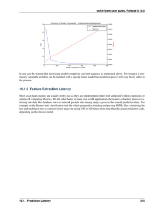


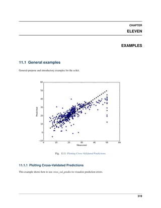
![scikit-learn user guide, Release 0.16.0
Python source code: plot_cv_predict.py
from sklearn import datasets
from sklearn.cross_validation import cross_val_predict
from sklearn import linear_model
import matplotlib.pyplot as plt
lr = linear_model.LinearRegression()
boston = datasets.load_boston()
y = boston.target
# cross_val_predict returns an array of the same size as `y` where each entry
# is a prediction obtained by cross validated:
predicted = cross_val_predict(lr, boston.data, y, cv=10)
fig,ax = plt.subplots()
ax.scatter(y, predicted)
ax.plot([y.min(), y.max()], [y.min(), y.max()], 'k--', lw=4)
ax.set_xlabel('Measured')
ax.set_ylabel('Predicted')
fig.show()
Total running time of the example: 2.95 seconds ( 0 minutes 2.95 seconds)
320 Chapter 11. Examples](https://image.slidesharecdn.com/scikit-learn0-150409112902-conversion-gate01/85/Scikit-learn-0-16-0-user-guide-330-320.jpg)
![scikit-learn user guide, Release 0.16.0
Fig. 11.2: Concatenating multiple feature extraction methods
11.1.2 Concatenating multiple feature extraction methods
In many real-world examples, there are many ways to extract features from a dataset. Often it is beneficial to combine
several methods to obtain good performance. This example shows how to use FeatureUnion to combine features
obtained by PCA and univariate selection.
Combining features using this transformer has the benefit that it allows cross validation and grid searches over the
whole process.
The combination used in this example is not particularly helpful on this dataset and is only used to illustrate the usage
of FeatureUnion.
Python source code: feature_stacker.py
# Author: Andreas Mueller <amueller@ais.uni-bonn.de>
#
# License: BSD 3 clause
from sklearn.pipeline import Pipeline, FeatureUnion
from sklearn.grid_search import GridSearchCV
from sklearn.svm import SVC
from sklearn.datasets import load_iris
from sklearn.decomposition import PCA
from sklearn.feature_selection import SelectKBest
iris = load_iris()
X, y = iris.data, iris.target
# This dataset is way to high-dimensional. Better do PCA:
pca = PCA(n_components=2)
# Maybe some original features where good, too?
selection = SelectKBest(k=1)
# Build estimator from PCA and Univariate selection:
combined_features = FeatureUnion([("pca", pca), ("univ_select", selection)])
# Use combined features to transform dataset:
X_features = combined_features.fit(X, y).transform(X)
svm = SVC(kernel="linear")
11.1. General examples 321](https://image.slidesharecdn.com/scikit-learn0-150409112902-conversion-gate01/85/Scikit-learn-0-16-0-user-guide-331-320.jpg)
![scikit-learn user guide, Release 0.16.0
# Do grid search over k, n_components and C:
pipeline = Pipeline([("features", combined_features), ("svm", svm)])
param_grid = dict(features__pca__n_components=[1, 2, 3],
features__univ_select__k=[1, 2],
svm__C=[0.1, 1, 10])
grid_search = GridSearchCV(pipeline, param_grid=param_grid, verbose=10)
grid_search.fit(X, y)
print(grid_search.best_estimator_)
Fig. 11.3: Isotonic Regression
11.1.3 Isotonic Regression
An illustration of the isotonic regression on generated data. The isotonic regression finds a non-decreasing approx-
imation of a function while minimizing the mean squared error on the training data. The benefit of such a model is
that it does not assume any form for the target function such as linearity. For comparison a linear regression is also
presented.
322 Chapter 11. Examples](https://image.slidesharecdn.com/scikit-learn0-150409112902-conversion-gate01/85/Scikit-learn-0-16-0-user-guide-332-320.jpg)

![scikit-learn user guide, Release 0.16.0
y_ = ir.fit_transform(x, y)
lr = LinearRegression()
lr.fit(x[:, np.newaxis], y) # x needs to be 2d for LinearRegression
###############################################################################
# plot result
segments = [[[i, y[i]], [i, y_[i]]] for i in range(n)]
lc = LineCollection(segments, zorder=0)
lc.set_array(np.ones(len(y)))
lc.set_linewidths(0.5 * np.ones(n))
fig = plt.figure()
plt.plot(x, y, 'r.', markersize=12)
plt.plot(x, y_, 'g.-', markersize=12)
plt.plot(x, lr.predict(x[:, np.newaxis]), 'b-')
plt.gca().add_collection(lc)
plt.legend(('Data', 'Isotonic Fit', 'Linear Fit'), loc='lower right')
plt.title('Isotonic regression')
plt.show()
Total running time of the example: 0.05 seconds ( 0 minutes 0.05 seconds)
Fig. 11.4: Imputing missing values before building an estimator
11.1.4 Imputing missing values before building an estimator
This example shows that imputing the missing values can give better results than discarding the samples containing
any missing value. Imputing does not always improve the predictions, so please check via cross-validation. Sometimes
dropping rows or using marker values is more effective.
Missing values can be replaced by the mean, the median or the most frequent value using the strategy hyper-
parameter. The median is a more robust estimator for data with high magnitude variables which could dominate
results (otherwise known as a ‘long tail’).
Script output:
Score with the entire dataset = 0.56
Score without the samples containing missing values = 0.48
Score after imputation of the missing values = 0.55
In this case, imputing helps the classifier get close to the original score.
324 Chapter 11. Examples](https://image.slidesharecdn.com/scikit-learn0-150409112902-conversion-gate01/85/Scikit-learn-0-16-0-user-guide-334-320.jpg)
![scikit-learn user guide, Release 0.16.0
Python source code: missing_values.py
import numpy as np
from sklearn.datasets import load_boston
from sklearn.ensemble import RandomForestRegressor
from sklearn.pipeline import Pipeline
from sklearn.preprocessing import Imputer
from sklearn.cross_validation import cross_val_score
rng = np.random.RandomState(0)
dataset = load_boston()
X_full, y_full = dataset.data, dataset.target
n_samples = X_full.shape[0]
n_features = X_full.shape[1]
# Estimate the score on the entire dataset, with no missing values
estimator = RandomForestRegressor(random_state=0, n_estimators=100)
score = cross_val_score(estimator, X_full, y_full).mean()
print("Score with the entire dataset = %.2f" % score)
# Add missing values in 75% of the lines
missing_rate = 0.75
n_missing_samples = np.floor(n_samples * missing_rate)
missing_samples = np.hstack((np.zeros(n_samples - n_missing_samples,
dtype=np.bool),
np.ones(n_missing_samples,
dtype=np.bool)))
rng.shuffle(missing_samples)
missing_features = rng.randint(0, n_features, n_missing_samples)
# Estimate the score without the lines containing missing values
X_filtered = X_full[~missing_samples, :]
y_filtered = y_full[~missing_samples]
estimator = RandomForestRegressor(random_state=0, n_estimators=100)
score = cross_val_score(estimator, X_filtered, y_filtered).mean()
print("Score without the samples containing missing values = %.2f" % score)
# Estimate the score after imputation of the missing values
X_missing = X_full.copy()
X_missing[np.where(missing_samples)[0], missing_features] = 0
y_missing = y_full.copy()
estimator = Pipeline([("imputer", Imputer(missing_values=0,
strategy="mean",
axis=0)),
("forest", RandomForestRegressor(random_state=0,
n_estimators=100))])
score = cross_val_score(estimator, X_missing, y_missing).mean()
print("Score after imputation of the missing values = %.2f" % score)
11.1.5 Pipelining: chaining a PCA and a logistic regression
The PCA does an unsupervised dimensionality reduction, while the logistic regression does the prediction.
We use a GridSearchCV to set the dimensionality of the PCA
11.1. General examples 325](https://image.slidesharecdn.com/scikit-learn0-150409112902-conversion-gate01/85/Scikit-learn-0-16-0-user-guide-335-320.jpg)

![scikit-learn user guide, Release 0.16.0
import numpy as np
import matplotlib.pyplot as plt
from sklearn import linear_model, decomposition, datasets
from sklearn.pipeline import Pipeline
from sklearn.grid_search import GridSearchCV
logistic = linear_model.LogisticRegression()
pca = decomposition.PCA()
pipe = Pipeline(steps=[('pca', pca), ('logistic', logistic)])
digits = datasets.load_digits()
X_digits = digits.data
y_digits = digits.target
###############################################################################
# Plot the PCA spectrum
pca.fit(X_digits)
plt.figure(1, figsize=(4, 3))
plt.clf()
plt.axes([.2, .2, .7, .7])
plt.plot(pca.explained_variance_, linewidth=2)
plt.axis('tight')
plt.xlabel('n_components')
plt.ylabel('explained_variance_')
###############################################################################
# Prediction
n_components = [20, 40, 64]
Cs = np.logspace(-4, 4, 3)
#Parameters of pipelines can be set using ‘__’ separated parameter names:
estimator = GridSearchCV(pipe,
dict(pca__n_components=n_components,
logistic__C=Cs))
estimator.fit(X_digits, y_digits)
plt.axvline(estimator.best_estimator_.named_steps['pca'].n_components,
linestyle=':', label='n_components chosen')
plt.legend(prop=dict(size=12))
plt.show()
Total running time of the example: 6.49 seconds ( 0 minutes 6.49 seconds)
11.1.6 Multilabel classification
This example simulates a multi-label document classification problem. The dataset is generated randomly based on
the following process:
• pick the number of labels: n ~ Poisson(n_labels)
• n times, choose a class c: c ~ Multinomial(theta)
• pick the document length: k ~ Poisson(length)
11.1. General examples 327](https://image.slidesharecdn.com/scikit-learn0-150409112902-conversion-gate01/85/Scikit-learn-0-16-0-user-guide-337-320.jpg)
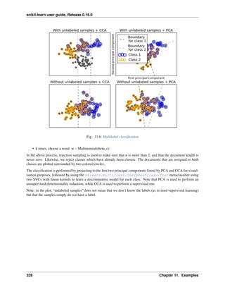
![scikit-learn user guide, Release 0.16.0
Python source code: plot_multilabel.py
print(__doc__)
import numpy as np
import matplotlib.pyplot as plt
from sklearn.datasets import make_multilabel_classification
from sklearn.multiclass import OneVsRestClassifier
from sklearn.svm import SVC
from sklearn.preprocessing import LabelBinarizer
from sklearn.decomposition import PCA
from sklearn.cross_decomposition import CCA
def plot_hyperplane(clf, min_x, max_x, linestyle, label):
# get the separating hyperplane
w = clf.coef_[0]
a = -w[0] / w[1]
xx = np.linspace(min_x - 5, max_x + 5) # make sure the line is long enough
yy = a * xx - (clf.intercept_[0]) / w[1]
plt.plot(xx, yy, linestyle, label=label)
def plot_subfigure(X, Y, subplot, title, transform):
if transform == "pca":
11.1. General examples 329](https://image.slidesharecdn.com/scikit-learn0-150409112902-conversion-gate01/85/Scikit-learn-0-16-0-user-guide-339-320.jpg)
![scikit-learn user guide, Release 0.16.0
X = PCA(n_components=2).fit_transform(X)
elif transform == "cca":
X = CCA(n_components=2).fit(X, Y).transform(X)
else:
raise ValueError
min_x = np.min(X[:, 0])
max_x = np.max(X[:, 0])
min_y = np.min(X[:, 1])
max_y = np.max(X[:, 1])
classif = OneVsRestClassifier(SVC(kernel='linear'))
classif.fit(X, Y)
plt.subplot(2, 2, subplot)
plt.title(title)
zero_class = np.where(Y[:, 0])
one_class = np.where(Y[:, 1])
plt.scatter(X[:, 0], X[:, 1], s=40, c='gray')
plt.scatter(X[zero_class, 0], X[zero_class, 1], s=160, edgecolors='b',
facecolors='none', linewidths=2, label='Class 1')
plt.scatter(X[one_class, 0], X[one_class, 1], s=80, edgecolors='orange',
facecolors='none', linewidths=2, label='Class 2')
plot_hyperplane(classif.estimators_[0], min_x, max_x, 'k--',
'Boundarynfor class 1')
plot_hyperplane(classif.estimators_[1], min_x, max_x, 'k-.',
'Boundarynfor class 2')
plt.xticks(())
plt.yticks(())
plt.xlim(min_x - .5 * max_x, max_x + .5 * max_x)
plt.ylim(min_y - .5 * max_y, max_y + .5 * max_y)
if subplot == 2:
plt.xlabel('First principal component')
plt.ylabel('Second principal component')
plt.legend(loc="upper left")
plt.figure(figsize=(8, 6))
X, Y = make_multilabel_classification(n_classes=2, n_labels=1,
allow_unlabeled=True,
return_indicator=True,
random_state=1)
plot_subfigure(X, Y, 1, "With unlabeled samples + CCA", "cca")
plot_subfigure(X, Y, 2, "With unlabeled samples + PCA", "pca")
X, Y = make_multilabel_classification(n_classes=2, n_labels=1,
allow_unlabeled=False,
return_indicator=True,
random_state=1)
plot_subfigure(X, Y, 3, "Without unlabeled samples + CCA", "cca")
plot_subfigure(X, Y, 4, "Without unlabeled samples + PCA", "pca")
330 Chapter 11. Examples](https://image.slidesharecdn.com/scikit-learn0-150409112902-conversion-gate01/85/Scikit-learn-0-16-0-user-guide-340-320.jpg)


![scikit-learn user guide, Release 0.16.0
from sklearn.ensemble import ExtraTreesRegressor
from sklearn.neighbors import KNeighborsRegressor
from sklearn.linear_model import LinearRegression
from sklearn.linear_model import RidgeCV
# Load the faces datasets
data = fetch_olivetti_faces()
targets = data.target
data = data.images.reshape((len(data.images), -1))
train = data[targets < 30]
test = data[targets >= 30] # Test on independent people
# Test on a subset of people
n_faces = 5
rng = check_random_state(4)
face_ids = rng.randint(test.shape[0], size=(n_faces, ))
test = test[face_ids, :]
n_pixels = data.shape[1]
X_train = train[:, :np.ceil(0.5 * n_pixels)] # Upper half of the faces
y_train = train[:, np.floor(0.5 * n_pixels):] # Lower half of the faces
X_test = test[:, :np.ceil(0.5 * n_pixels)]
y_test = test[:, np.floor(0.5 * n_pixels):]
# Fit estimators
ESTIMATORS = {
"Extra trees": ExtraTreesRegressor(n_estimators=10, max_features=32,
random_state=0),
"K-nn": KNeighborsRegressor(),
"Linear regression": LinearRegression(),
"Ridge": RidgeCV(),
}
y_test_predict = dict()
for name, estimator in ESTIMATORS.items():
estimator.fit(X_train, y_train)
y_test_predict[name] = estimator.predict(X_test)
# Plot the completed faces
image_shape = (64, 64)
n_cols = 1 + len(ESTIMATORS)
plt.figure(figsize=(2. * n_cols, 2.26 * n_faces))
plt.suptitle("Face completion with multi-output estimators", size=16)
for i in range(n_faces):
true_face = np.hstack((X_test[i], y_test[i]))
if i:
sub = plt.subplot(n_faces, n_cols, i * n_cols + 1)
else:
sub = plt.subplot(n_faces, n_cols, i * n_cols + 1,
title="true faces")
sub.axis("off")
sub.imshow(true_face.reshape(image_shape),
11.1. General examples 333](https://image.slidesharecdn.com/scikit-learn0-150409112902-conversion-gate01/85/Scikit-learn-0-16-0-user-guide-343-320.jpg)
![scikit-learn user guide, Release 0.16.0
cmap=plt.cm.gray,
interpolation="nearest")
for j, est in enumerate(sorted(ESTIMATORS)):
completed_face = np.hstack((X_test[i], y_test_predict[est][i]))
if i:
sub = plt.subplot(n_faces, n_cols, i * n_cols + 2 + j)
else:
sub = plt.subplot(n_faces, n_cols, i * n_cols + 2 + j,
title=est)
sub.axis("off")
sub.imshow(completed_face.reshape(image_shape),
cmap=plt.cm.gray,
interpolation="nearest")
plt.show()
Total running time of the example: 58.20 seconds ( 0 minutes 58.20 seconds)
Fig. 11.8: The Johnson-Lindenstrauss bound for embedding with random projections
11.1.8 The Johnson-Lindenstrauss bound for embedding with random projections
The Johnson-Lindenstrauss lemma states that any high dimensional dataset can be randomly projected into a lower
dimensional Euclidean space while controlling the distortion in the pairwise distances.
334 Chapter 11. Examples](https://image.slidesharecdn.com/scikit-learn0-150409112902-conversion-gate01/85/Scikit-learn-0-16-0-user-guide-344-320.jpg)
![scikit-learn user guide, Release 0.16.0
Theoretical bounds
The distortion introduced by a random projection p is asserted by the fact that p is defining an eps-embedding with
good probability as defined by:
(1 - eps) ||u - v||^2 < ||p(u) - p(v)||^2 < (1 + eps) ||u - v||^2
Where u and v are any rows taken from a dataset of shape [n_samples, n_features] and p is a projection by a random
Gaussian N(0, 1) matrix with shape [n_components, n_features] (or a sparse Achlioptas matrix).
The minimum number of components to guarantees the eps-embedding is given by:
n_components >= 4 log(n_samples) / (eps^2 / 2 - eps^3 / 3)
The first plot shows that with an increasing number of samples n_samples, the minimal number of dimensions
n_components increased logarithmically in order to guarantee an eps-embedding.
The second plot shows that an increase of the admissible distortion eps allows to reduce drastically the minimal
number of dimensions n_components for a given number of samples n_samples
Empirical validation
We validate the above bounds on the the digits dataset or on the 20 newsgroups text document (TF-IDF word frequen-
cies) dataset:
• for the digits dataset, some 8x8 gray level pixels data for 500 handwritten digits pictures are randomly projected
to spaces for various larger number of dimensions n_components.
• for the 20 newsgroups dataset some 500 documents with 100k features in total are projected using a
sparse random matrix to smaller euclidean spaces with various values for the target number of dimensions
n_components.
The default dataset is the digits dataset. To run the example on the twenty newsgroups dataset, pass the –twenty-
newsgroups command line argument to this script.
For each value of n_components, we plot:
• 2D distribution of sample pairs with pairwise distances in original and projected spaces as x and y axis respec-
tively.
• 1D histogram of the ratio of those distances (projected / original).
We can see that for low values of n_components the distribution is wide with many distorted pairs and a skewed
distribution (due to the hard limit of zero ratio on the left as distances are always positives) while for larger values of
n_components the distortion is controlled and the distances are well preserved by the random projection.
Remarks
According to the JL lemma, projecting 500 samples without too much distortion will require at least several thousands
dimensions, irrespective of the number of features of the original dataset.
Hence using random projections on the digits dataset which only has 64 features in the input space does not make
sense: it does not allow for dimensionality reduction in this case.
On the twenty newsgroups on the other hand the dimensionality can be decreased from 56436 down to 10000 while
reasonably preserving pairwise distances.
11.1. General examples 335](https://image.slidesharecdn.com/scikit-learn0-150409112902-conversion-gate01/85/Scikit-learn-0-16-0-user-guide-345-320.jpg)


![scikit-learn user guide, Release 0.16.0
Script output:
Embedding 500 samples with dim 64 using various random projections
Projected 500 samples from 64 to 300 in 0.007s
Random matrix with size: 0.028MB
Mean distances rate: 0.96 (0.08)
Projected 500 samples from 64 to 1000 in 0.018s
Random matrix with size: 0.095MB
Mean distances rate: 0.99 (0.05)
Projected 500 samples from 64 to 10000 in 0.274s
Random matrix with size: 0.961MB
Mean distances rate: 1.01 (0.01)
Python source code: plot_johnson_lindenstrauss_bound.py
print(__doc__)
import sys
from time import time
import numpy as np
import matplotlib.pyplot as plt
from sklearn.random_projection import johnson_lindenstrauss_min_dim
from sklearn.random_projection import SparseRandomProjection
from sklearn.datasets import fetch_20newsgroups_vectorized
from sklearn.datasets import load_digits
from sklearn.metrics.pairwise import euclidean_distances
# Part 1: plot the theoretical dependency between n_components_min and
# n_samples
# range of admissible distortions
eps_range = np.linspace(0.1, 0.99, 5)
colors = plt.cm.Blues(np.linspace(0.3, 1.0, len(eps_range)))
# range of number of samples (observation) to embed
n_samples_range = np.logspace(1, 9, 9)
plt.figure()
for eps, color in zip(eps_range, colors):
min_n_components = johnson_lindenstrauss_min_dim(n_samples_range, eps=eps)
plt.loglog(n_samples_range, min_n_components, color=color)
plt.legend(["eps = %0.1f" % eps for eps in eps_range], loc="lower right")
plt.xlabel("Number of observations to eps-embed")
plt.ylabel("Minimum number of dimensions")
plt.title("Johnson-Lindenstrauss bounds:nn_samples vs n_components")
# range of admissible distortions
eps_range = np.linspace(0.01, 0.99, 100)
# range of number of samples (observation) to embed
n_samples_range = np.logspace(2, 6, 5)
colors = plt.cm.Blues(np.linspace(0.3, 1.0, len(n_samples_range)))
plt.figure()
for n_samples, color in zip(n_samples_range, colors):
min_n_components = johnson_lindenstrauss_min_dim(n_samples, eps=eps_range)
plt.semilogy(eps_range, min_n_components, color=color)
338 Chapter 11. Examples](https://image.slidesharecdn.com/scikit-learn0-150409112902-conversion-gate01/85/Scikit-learn-0-16-0-user-guide-348-320.jpg)
![scikit-learn user guide, Release 0.16.0
plt.legend(["n_samples = %d" % n for n in n_samples_range], loc="upper right")
plt.xlabel("Distortion eps")
plt.ylabel("Minimum number of dimensions")
plt.title("Johnson-Lindenstrauss bounds:nn_components vs eps")
# Part 2: perform sparse random projection of some digits images which are
# quite low dimensional and dense or documents of the 20 newsgroups dataset
# which is both high dimensional and sparse
if '--twenty-newsgroups' in sys.argv:
# Need an internet connection hence not enabled by default
data = fetch_20newsgroups_vectorized().data[:500]
else:
data = load_digits().data[:500]
n_samples, n_features = data.shape
print("Embedding %d samples with dim %d using various random projections"
% (n_samples, n_features))
n_components_range = np.array([300, 1000, 10000])
dists = euclidean_distances(data, squared=True).ravel()
# select only non-identical samples pairs
nonzero = dists != 0
dists = dists[nonzero]
for n_components in n_components_range:
t0 = time()
rp = SparseRandomProjection(n_components=n_components)
projected_data = rp.fit_transform(data)
print("Projected %d samples from %d to %d in %0.3fs"
% (n_samples, n_features, n_components, time() - t0))
if hasattr(rp, 'components_'):
n_bytes = rp.components_.data.nbytes
n_bytes += rp.components_.indices.nbytes
print("Random matrix with size: %0.3fMB" % (n_bytes / 1e6))
projected_dists = euclidean_distances(
projected_data, squared=True).ravel()[nonzero]
plt.figure()
plt.hexbin(dists, projected_dists, gridsize=100, cmap=plt.cm.PuBu)
plt.xlabel("Pairwise squared distances in original space")
plt.ylabel("Pairwise squared distances in projected space")
plt.title("Pairwise distances distribution for n_components=%d" %
n_components)
cb = plt.colorbar()
cb.set_label('Sample pairs counts')
rates = projected_dists / dists
print("Mean distances rate: %0.2f (%0.2f)"
% (np.mean(rates), np.std(rates)))
plt.figure()
plt.hist(rates, bins=50, normed=True, range=(0., 2.))
plt.xlabel("Squared distances rate: projected / original")
plt.ylabel("Distribution of samples pairs")
plt.title("Histogram of pairwise distance rates for n_components=%d" %
11.1. General examples 339](https://image.slidesharecdn.com/scikit-learn0-150409112902-conversion-gate01/85/Scikit-learn-0-16-0-user-guide-349-320.jpg)


![scikit-learn user guide, Release 0.16.0
# Authors: Jan Hendrik Metzen <jhm@informatik.uni-bremen.de>
# License: BSD 3 clause
from __future__ import division
import time
import numpy as np
from sklearn.svm import SVR
from sklearn.grid_search import GridSearchCV
from sklearn.learning_curve import learning_curve
from sklearn.kernel_ridge import KernelRidge
import matplotlib.pyplot as plt
rng = np.random.RandomState(0)
#############################################################################
# Generate sample data
X = 5 * rng.rand(10000, 1)
y = np.sin(X).ravel()
# Add noise to targets
y[::5] += 3 * (0.5 - rng.rand(X.shape[0]/5))
X_plot = np.linspace(0, 5, 100000)[:, None]
#############################################################################
# Fit regression model
train_size = 100
svr = GridSearchCV(SVR(kernel='rbf', gamma=0.1), cv=5,
param_grid={"C": [1e0, 1e1, 1e2, 1e3],
"gamma": np.logspace(-2, 2, 5)})
kr = GridSearchCV(KernelRidge(kernel='rbf', gamma=0.1), cv=5,
param_grid={"alpha": [1e0, 0.1, 1e-2, 1e-3],
"gamma": np.logspace(-2, 2, 5)})
t0 = time.time()
svr.fit(X[:train_size], y[:train_size])
svr_fit = time.time() - t0
print("SVR complexity and bandwidth selected and model fitted in %.3f s"
% svr_fit)
t0 = time.time()
kr.fit(X[:train_size], y[:train_size])
kr_fit = time.time() - t0
print("KRR complexity and bandwidth selected and model fitted in %.3f s"
% kr_fit)
sv_ratio = svr.best_estimator_.support_.shape[0] / train_size
print("Support vector ratio: %.3f" % sv_ratio)
t0 = time.time()
y_svr = svr.predict(X_plot)
svr_predict = time.time() - t0
print("SVR prediction for %d inputs in %.3f s"
% (X_plot.shape[0], svr_predict))
342 Chapter 11. Examples](https://image.slidesharecdn.com/scikit-learn0-150409112902-conversion-gate01/85/Scikit-learn-0-16-0-user-guide-352-320.jpg)
![scikit-learn user guide, Release 0.16.0
t0 = time.time()
y_kr = kr.predict(X_plot)
kr_predict = time.time() - t0
print("KRR prediction for %d inputs in %.3f s"
% (X_plot.shape[0], kr_predict))
#############################################################################
# look at the results
sv_ind = svr.best_estimator_.support_
plt.scatter(X[sv_ind], y[sv_ind], c='r', s=50, label='SVR support vectors')
plt.scatter(X[:100], y[:100], c='k', label='data')
plt.hold('on')
plt.plot(X_plot, y_svr, c='r',
label='SVR (fit: %.3fs, predict: %.3fs)' % (svr_fit, svr_predict))
plt.plot(X_plot, y_kr, c='g',
label='KRR (fit: %.3fs, predict: %.3fs)' % (kr_fit, kr_predict))
plt.xlabel('data')
plt.ylabel('target')
plt.title('SVR versus Kernel Ridge')
plt.legend()
# Visualize training and prediction time
plt.figure()
# Generate sample data
X = 5 * rng.rand(10000, 1)
y = np.sin(X).ravel()
y[::5] += 3 * (0.5 - rng.rand(X.shape[0]/5))
sizes = np.logspace(1, 4, 7)
for name, estimator in {"KRR": KernelRidge(kernel='rbf', alpha=0.1,
gamma=10),
"SVR": SVR(kernel='rbf', C=1e1, gamma=10)}.items():
train_time = []
test_time = []
for train_test_size in sizes:
t0 = time.time()
estimator.fit(X[:train_test_size], y[:train_test_size])
train_time.append(time.time() - t0)
t0 = time.time()
estimator.predict(X_plot[:1000])
test_time.append(time.time() - t0)
plt.plot(sizes, train_time, 'o-', color="r" if name == "SVR" else "g",
label="%s (train)" % name)
plt.plot(sizes, test_time, 'o--', color="r" if name == "SVR" else "g",
label="%s (test)" % name)
plt.xscale("log")
plt.yscale("log")
plt.xlabel("Train size")
plt.ylabel("Time (seconds)")
plt.title('Execution Time')
plt.legend(loc="best")
# Visualize learning curves
plt.figure()
11.1. General examples 343](https://image.slidesharecdn.com/scikit-learn0-150409112902-conversion-gate01/85/Scikit-learn-0-16-0-user-guide-353-320.jpg)
![scikit-learn user guide, Release 0.16.0
svr = SVR(kernel='rbf', C=1e1, gamma=0.1)
kr = KernelRidge(kernel='rbf', alpha=0.1, gamma=0.1)
train_sizes, train_scores_svr, test_scores_svr =
learning_curve(svr, X[:100], y[:100], train_sizes=np.linspace(0.1, 1, 10),
scoring="mean_squared_error", cv=10)
train_sizes_abs, train_scores_kr, test_scores_kr =
learning_curve(kr, X[:100], y[:100], train_sizes=np.linspace(0.1, 1, 10),
scoring="mean_squared_error", cv=10)
plt.plot(train_sizes, test_scores_svr.mean(1), 'o-', color="r",
label="SVR")
plt.plot(train_sizes, test_scores_kr.mean(1), 'o-', color="g",
label="KRR")
plt.xlabel("Train size")
plt.ylabel("Mean Squared Error")
plt.title('Learning curves')
plt.legend(loc="best")
plt.show()
Total running time of the example: 49.29 seconds ( 0 minutes 49.29 seconds)
Fig. 11.10: Feature Union with Heterogeneous Data Sources
11.1.10 Feature Union with Heterogeneous Data Sources
Datasets can often contain components of that require different feature extraction and processing pipelines. This
scenario might occur when:
1. Your dataset consists of heterogeneous data types (e.g. raster images and text captions)
2. Your dataset is stored in a Pandas DataFrame and different columns require different processing pipelines.
This example demonstrates how to use sklearn.feature_extraction.FeatureUnion on a dataset con-
taining different types of features. We use the 20-newsgroups dataset and compute standard bag-of-words features for
the subject line and body in separate pipelines as well as ad hoc features on the body. We combine them (with weights)
using a FeatureUnion and finally train a classifier on the combined set of features.
The choice of features is not particularly helpful, but serves to illustrate the technique.
Python source code: hetero_feature_union.py
344 Chapter 11. Examples](https://image.slidesharecdn.com/scikit-learn0-150409112902-conversion-gate01/85/Scikit-learn-0-16-0-user-guide-354-320.jpg)
![scikit-learn user guide, Release 0.16.0
# Author: Matt Terry <matt.terry@gmail.com>
#
# License: BSD 3 clause
from __future__ import print_function
import numpy as np
from sklearn.base import BaseEstimator, TransformerMixin
from sklearn.datasets import fetch_20newsgroups
from sklearn.datasets.twenty_newsgroups import strip_newsgroup_footer
from sklearn.datasets.twenty_newsgroups import strip_newsgroup_quoting
from sklearn.decomposition import TruncatedSVD
from sklearn.feature_extraction import DictVectorizer
from sklearn.feature_extraction.text import TfidfVectorizer
from sklearn.metrics import classification_report
from sklearn.pipeline import FeatureUnion
from sklearn.pipeline import Pipeline
from sklearn.svm import SVC
class ItemSelector(BaseEstimator, TransformerMixin):
"""For data grouped by feature, select subset of data at a provided key.
The data is expected to be stored in a 2D data structure, where the first
index is over features and the second is over samples. i.e.
>> len(data[key]) == n_samples
Please note that this is the opposite convention to sklearn feature
matrixes (where the first index corresponds to sample).
ItemSelector only requires that the collection implement getitem
(data[key]). Examples include: a dict of lists, 2D numpy array, Pandas
DataFrame, numpy record array, etc.
>> data = {'a': [1, 5, 2, 5, 2, 8],
'b': [9, 4, 1, 4, 1, 3]}
>> ds = ItemSelector(key='a')
>> data['a'] == ds.transform(data)
ItemSelector is not designed to handle data grouped by sample. (e.g. a
list of dicts). If your data is structured this way, consider a
transformer along the lines of `sklearn.feature_extraction.DictVectorizer`.
Parameters
----------
key : hashable, required
The key corresponding to the desired value in a mappable.
"""
def __init__(self, key):
self.key = key
def fit(self, x, y=None):
return self
def transform(self, data_dict):
return data_dict[self.key]
11.1. General examples 345](https://image.slidesharecdn.com/scikit-learn0-150409112902-conversion-gate01/85/Scikit-learn-0-16-0-user-guide-355-320.jpg)
![scikit-learn user guide, Release 0.16.0
class TextStats(BaseEstimator, TransformerMixin):
"""Extract features from each document for DictVectorizer"""
def fit(self, x, y=None):
return self
def transform(self, posts):
return [{'length': len(text),
'num_sentences': text.count('.')}
for text in posts]
class SubjectBodyExtractor(BaseEstimator, TransformerMixin):
"""Extract the subject & body from a usenet post in a single pass.
Takes a sequence of strings and produces a dict of sequences. Keys are
`subject` and `body`.
"""
def fit(self, x, y=None):
return self
def transform(self, posts):
features = np.recarray(shape=(len(posts),),
dtype=[('subject', object), ('body', object)])
for i, text in enumerate(posts):
headers, _, bod = text.partition('nn')
bod = strip_newsgroup_footer(bod)
bod = strip_newsgroup_quoting(bod)
features['body'][i] = bod
prefix = 'Subject:'
sub = ''
for line in headers.split('n'):
if line.startswith(prefix):
sub = line[len(prefix):]
break
features['subject'][i] = sub
return features
pipeline = Pipeline([
# Extract the subject & body
('subjectbody', SubjectBodyExtractor()),
# Use FeatureUnion to combine the features from subject and body
('union', FeatureUnion(
transformer_list=[
# Pipeline for pulling features from the post's subject line
('subject', Pipeline([
('selector', ItemSelector(key='subject')),
('tfidf', TfidfVectorizer(min_df=50)),
])),
# Pipeline for standard bag-of-words model for body
('body_bow', Pipeline([
('selector', ItemSelector(key='body')),
346 Chapter 11. Examples](https://image.slidesharecdn.com/scikit-learn0-150409112902-conversion-gate01/85/Scikit-learn-0-16-0-user-guide-356-320.jpg)
![scikit-learn user guide, Release 0.16.0
('tfidf', TfidfVectorizer()),
('best', TruncatedSVD(n_components=50)),
])),
# Pipeline for pulling ad hoc features from post's body
('body_stats', Pipeline([
('selector', ItemSelector(key='body')),
('stats', TextStats()), # returns a list of dicts
('vect', DictVectorizer()), # list of dicts -> feature matrix
])),
],
# weight components in FeatureUnion
transformer_weights={
'subject': 0.8,
'body_bow': 0.5,
'body_stats': 1.0,
},
)),
# Use a SVC classifier on the combined features
('svc', SVC(kernel='linear')),
])
# limit the list of categories to make running this exmaple faster.
categories = ['alt.atheism', 'talk.religion.misc']
train = fetch_20newsgroups(random_state=1,
subset='train',
categories=categories,
)
test = fetch_20newsgroups(random_state=1,
subset='test',
categories=categories,
)
pipeline.fit(train.data, train.target)
y = pipeline.predict(test.data)
print(classification_report(y, test.target))
11.1.11 Explicit feature map approximation for RBF kernels
An example illustrating the approximation of the feature map of an RBF kernel.
It shows how to use RBFSampler and Nystroem to approximate the feature map of an RBF kernel for classification
with an SVM on the digits dataset. Results using a linear SVM in the original space, a linear SVM using the approx-
imate mappings and using a kernelized SVM are compared. Timings and accuracy for varying amounts of Monte
Carlo samplings (in the case of RBFSampler, which uses random Fourier features) and different sized subsets of the
training set (for Nystroem) for the approximate mapping are shown.
Please note that the dataset here is not large enough to show the benefits of kernel approximation, as the exact SVM is
still reasonably fast.
Sampling more dimensions clearly leads to better classification results, but comes at a greater cost. This means there
is a tradeoff between runtime and accuracy, given by the parameter n_components. Note that solving the Linear
SVM and also the approximate kernel SVM could be greatly accelerated by using stochastic gradient descent via
sklearn.linear_model.SGDClassifier. This is not easily possible for the case of the kernelized SVM.
11.1. General examples 347](https://image.slidesharecdn.com/scikit-learn0-150409112902-conversion-gate01/85/Scikit-learn-0-16-0-user-guide-357-320.jpg)
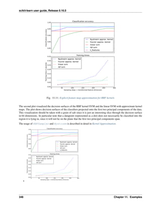
![scikit-learn user guide, Release 0.16.0
•
Python source code: plot_kernel_approximation.py
print(__doc__)
# Author: Gael Varoquaux <gael dot varoquaux at normalesup dot org>
# Andreas Mueller <amueller@ais.uni-bonn.de>
# License: BSD 3 clause
# Standard scientific Python imports
import matplotlib.pyplot as plt
import numpy as np
from time import time
# Import datasets, classifiers and performance metrics
from sklearn import datasets, svm, pipeline
from sklearn.kernel_approximation import (RBFSampler,
Nystroem)
from sklearn.decomposition import PCA
# The digits dataset
digits = datasets.load_digits(n_class=9)
# To apply an classifier on this data, we need to flatten the image, to
# turn the data in a (samples, feature) matrix:
n_samples = len(digits.data)
data = digits.data / 16.
data -= data.mean(axis=0)
# We learn the digits on the first half of the digits
data_train, targets_train = data[:n_samples / 2], digits.target[:n_samples / 2]
# Now predict the value of the digit on the second half:
data_test, targets_test = data[n_samples / 2:], digits.target[n_samples / 2:]
#data_test = scaler.transform(data_test)
# Create a classifier: a support vector classifier
kernel_svm = svm.SVC(gamma=.2)
linear_svm = svm.LinearSVC()
# create pipeline from kernel approximation
# and linear svm
feature_map_fourier = RBFSampler(gamma=.2, random_state=1)
feature_map_nystroem = Nystroem(gamma=.2, random_state=1)
fourier_approx_svm = pipeline.Pipeline([("feature_map", feature_map_fourier),
("svm", svm.LinearSVC())])
nystroem_approx_svm = pipeline.Pipeline([("feature_map", feature_map_nystroem),
("svm", svm.LinearSVC())])
11.1. General examples 349](https://image.slidesharecdn.com/scikit-learn0-150409112902-conversion-gate01/85/Scikit-learn-0-16-0-user-guide-359-320.jpg)
![scikit-learn user guide, Release 0.16.0
# fit and predict using linear and kernel svm:
kernel_svm_time = time()
kernel_svm.fit(data_train, targets_train)
kernel_svm_score = kernel_svm.score(data_test, targets_test)
kernel_svm_time = time() - kernel_svm_time
linear_svm_time = time()
linear_svm.fit(data_train, targets_train)
linear_svm_score = linear_svm.score(data_test, targets_test)
linear_svm_time = time() - linear_svm_time
sample_sizes = 30 * np.arange(1, 10)
fourier_scores = []
nystroem_scores = []
fourier_times = []
nystroem_times = []
for D in sample_sizes:
fourier_approx_svm.set_params(feature_map__n_components=D)
nystroem_approx_svm.set_params(feature_map__n_components=D)
start = time()
nystroem_approx_svm.fit(data_train, targets_train)
nystroem_times.append(time() - start)
start = time()
fourier_approx_svm.fit(data_train, targets_train)
fourier_times.append(time() - start)
fourier_score = fourier_approx_svm.score(data_test, targets_test)
nystroem_score = nystroem_approx_svm.score(data_test, targets_test)
nystroem_scores.append(nystroem_score)
fourier_scores.append(fourier_score)
# plot the results:
plt.figure(figsize=(8, 8))
accuracy = plt.subplot(211)
# second y axis for timeings
timescale = plt.subplot(212)
accuracy.plot(sample_sizes, nystroem_scores, label="Nystroem approx. kernel")
timescale.plot(sample_sizes, nystroem_times, '--',
label='Nystroem approx. kernel')
accuracy.plot(sample_sizes, fourier_scores, label="Fourier approx. kernel")
timescale.plot(sample_sizes, fourier_times, '--',
label='Fourier approx. kernel')
# horizontal lines for exact rbf and linear kernels:
accuracy.plot([sample_sizes[0], sample_sizes[-1]],
[linear_svm_score, linear_svm_score], label="linear svm")
timescale.plot([sample_sizes[0], sample_sizes[-1]],
[linear_svm_time, linear_svm_time], '--', label='linear svm')
accuracy.plot([sample_sizes[0], sample_sizes[-1]],
[kernel_svm_score, kernel_svm_score], label="rbf svm")
timescale.plot([sample_sizes[0], sample_sizes[-1]],
[kernel_svm_time, kernel_svm_time], '--', label='rbf svm')
350 Chapter 11. Examples](https://image.slidesharecdn.com/scikit-learn0-150409112902-conversion-gate01/85/Scikit-learn-0-16-0-user-guide-360-320.jpg)
![scikit-learn user guide, Release 0.16.0
# vertical line for dataset dimensionality = 64
accuracy.plot([64, 64], [0.7, 1], label="n_features")
# legends and labels
accuracy.set_title("Classification accuracy")
timescale.set_title("Training times")
accuracy.set_xlim(sample_sizes[0], sample_sizes[-1])
accuracy.set_xticks(())
accuracy.set_ylim(np.min(fourier_scores), 1)
timescale.set_xlabel("Sampling steps = transformed feature dimension")
accuracy.set_ylabel("Classification accuracy")
timescale.set_ylabel("Training time in seconds")
accuracy.legend(loc='best')
timescale.legend(loc='best')
# visualize the decision surface, projected down to the first
# two principal components of the dataset
pca = PCA(n_components=8).fit(data_train)
X = pca.transform(data_train)
# Gemerate grid along first two principal components
multiples = np.arange(-2, 2, 0.1)
# steps along first component
first = multiples[:, np.newaxis] * pca.components_[0, :]
# steps along second component
second = multiples[:, np.newaxis] * pca.components_[1, :]
# combine
grid = first[np.newaxis, :, :] + second[:, np.newaxis, :]
flat_grid = grid.reshape(-1, data.shape[1])
# title for the plots
titles = ['SVC with rbf kernel',
'SVC (linear kernel)n with Fourier rbf feature mapn'
'n_components=100',
'SVC (linear kernel)n with Nystroem rbf feature mapn'
'n_components=100']
plt.tight_layout()
plt.figure(figsize=(12, 5))
# predict and plot
for i, clf in enumerate((kernel_svm, nystroem_approx_svm,
fourier_approx_svm)):
# Plot the decision boundary. For that, we will assign a color to each
# point in the mesh [x_min, m_max]x[y_min, y_max].
plt.subplot(1, 3, i + 1)
Z = clf.predict(flat_grid)
# Put the result into a color plot
Z = Z.reshape(grid.shape[:-1])
plt.contourf(multiples, multiples, Z, cmap=plt.cm.Paired)
plt.axis('off')
# Plot also the training points
plt.scatter(X[:, 0], X[:, 1], c=targets_train, cmap=plt.cm.Paired)
plt.title(titles[i])
11.1. General examples 351](https://image.slidesharecdn.com/scikit-learn0-150409112902-conversion-gate01/85/Scikit-learn-0-16-0-user-guide-361-320.jpg)
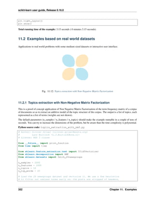
![scikit-learn user guide, Release 0.16.0
# footers and quoted replies, and common English words, words occurring in
# only one document or in at least 95% of the documents are removed.
t0 = time()
print("Loading dataset and extracting TF-IDF features...")
dataset = fetch_20newsgroups(shuffle=True, random_state=1,
remove=('headers', 'footers', 'quotes'))
vectorizer = TfidfVectorizer(max_df=0.95, min_df=2, max_features=n_features,
stop_words='english')
tfidf = vectorizer.fit_transform(dataset.data[:n_samples])
print("done in %0.3fs." % (time() - t0))
# Fit the NMF model
print("Fitting the NMF model with n_samples=%d and n_features=%d..."
% (n_samples, n_features))
nmf = NMF(n_components=n_topics, random_state=1).fit(tfidf)
print("done in %0.3fs." % (time() - t0))
feature_names = vectorizer.get_feature_names()
for topic_idx, topic in enumerate(nmf.components_):
print("Topic #%d:" % topic_idx)
print(" ".join([feature_names[i]
for i in topic.argsort()[:-n_top_words - 1:-1]]))
print()
Fig. 11.13: Outlier detection on a real data set
11.2. Examples based on real world datasets 353](https://image.slidesharecdn.com/scikit-learn0-150409112902-conversion-gate01/85/Scikit-learn-0-16-0-user-guide-363-320.jpg)

![scikit-learn user guide, Release 0.16.0
•
Python source code: plot_outlier_detection_housing.py
print(__doc__)
# Author: Virgile Fritsch <virgile.fritsch@inria.fr>
# License: BSD 3 clause
import numpy as np
from sklearn.covariance import EllipticEnvelope
from sklearn.svm import OneClassSVM
import matplotlib.pyplot as plt
import matplotlib.font_manager
from sklearn.datasets import load_boston
# Get data
X1 = load_boston()['data'][:, [8, 10]] # two clusters
X2 = load_boston()['data'][:, [5, 12]] # "banana"-shaped
# Define "classifiers" to be used
classifiers = {
"Empirical Covariance": EllipticEnvelope(support_fraction=1.,
contamination=0.261),
"Robust Covariance (Minimum Covariance Determinant)":
EllipticEnvelope(contamination=0.261),
"OCSVM": OneClassSVM(nu=0.261, gamma=0.05)}
colors = ['m', 'g', 'b']
legend1 = {}
legend2 = {}
# Learn a frontier for outlier detection with several classifiers
xx1, yy1 = np.meshgrid(np.linspace(-8, 28, 500), np.linspace(3, 40, 500))
xx2, yy2 = np.meshgrid(np.linspace(3, 10, 500), np.linspace(-5, 45, 500))
for i, (clf_name, clf) in enumerate(classifiers.items()):
plt.figure(1)
clf.fit(X1)
Z1 = clf.decision_function(np.c_[xx1.ravel(), yy1.ravel()])
Z1 = Z1.reshape(xx1.shape)
legend1[clf_name] = plt.contour(
xx1, yy1, Z1, levels=[0], linewidths=2, colors=colors[i])
plt.figure(2)
clf.fit(X2)
Z2 = clf.decision_function(np.c_[xx2.ravel(), yy2.ravel()])
Z2 = Z2.reshape(xx2.shape)
legend2[clf_name] = plt.contour(
11.2. Examples based on real world datasets 355](https://image.slidesharecdn.com/scikit-learn0-150409112902-conversion-gate01/85/Scikit-learn-0-16-0-user-guide-365-320.jpg)
![scikit-learn user guide, Release 0.16.0
xx2, yy2, Z2, levels=[0], linewidths=2, colors=colors[i])
legend1_values_list = list( legend1.values() )
legend1_keys_list = list( legend1.keys() )
# Plot the results (= shape of the data points cloud)
plt.figure(1) # two clusters
plt.title("Outlier detection on a real data set (boston housing)")
plt.scatter(X1[:, 0], X1[:, 1], color='black')
bbox_args = dict(boxstyle="round", fc="0.8")
arrow_args = dict(arrowstyle="->")
plt.annotate("several confounded points", xy=(24, 19),
xycoords="data", textcoords="data",
xytext=(13, 10), bbox=bbox_args, arrowprops=arrow_args)
plt.xlim((xx1.min(), xx1.max()))
plt.ylim((yy1.min(), yy1.max()))
plt.legend((legend1_values_list[0].collections[0],
legend1_values_list[1].collections[0],
legend1_values_list[2].collections[0]),
(legend1_keys_list[0], legend1_keys_list[1], legend1_keys_list[2]),
loc="upper center",
prop=matplotlib.font_manager.FontProperties(size=12))
plt.ylabel("accessibility to radial highways")
plt.xlabel("pupil-teacher ratio by town")
legend2_values_list = list( legend2.values() )
legend2_keys_list = list( legend2.keys() )
plt.figure(2) # "banana" shape
plt.title("Outlier detection on a real data set (boston housing)")
plt.scatter(X2[:, 0], X2[:, 1], color='black')
plt.xlim((xx2.min(), xx2.max()))
plt.ylim((yy2.min(), yy2.max()))
plt.legend((legend2_values_list[0].collections[0],
legend2_values_list[1].collections[0],
legend2_values_list[2].collections[0]),
(legend2_values_list[0], legend2_values_list[1], legend2_values_list[2]),
loc="upper center",
prop=matplotlib.font_manager.FontProperties(size=12))
plt.ylabel("% lower status of the population")
plt.xlabel("average number of rooms per dwelling")
plt.show()
Total running time of the example: 4.39 seconds ( 0 minutes 4.39 seconds)
11.2.3 Compressive sensing: tomography reconstruction with L1 prior (Lasso)
This example shows the reconstruction of an image from a set of parallel projections, acquired along different angles.
Such a dataset is acquired in computed tomography (CT).
Without any prior information on the sample, the number of projections required to reconstruct the image is of the
order of the linear size l of the image (in pixels). For simplicity we consider here a sparse image, where only pixels
on the boundary of objects have a non-zero value. Such data could correspond for example to a cellular material.
Note however that most images are sparse in a different basis, such as the Haar wavelets. Only l/7 projections are
acquired, therefore it is necessary to use prior information available on the sample (its sparsity): this is an example of
compressive sensing.
356 Chapter 11. Examples](https://image.slidesharecdn.com/scikit-learn0-150409112902-conversion-gate01/85/Scikit-learn-0-16-0-user-guide-366-320.jpg)

![scikit-learn user guide, Release 0.16.0
Python source code: plot_tomography_l1_reconstruction.py
print(__doc__)
# Author: Emmanuelle Gouillart <emmanuelle.gouillart@nsup.org>
# License: BSD 3 clause
import numpy as np
from scipy import sparse
from scipy import ndimage
from sklearn.linear_model import Lasso
from sklearn.linear_model import Ridge
import matplotlib.pyplot as plt
def _weights(x, dx=1, orig=0):
x = np.ravel(x)
floor_x = np.floor((x - orig) / dx)
alpha = (x - orig - floor_x * dx) / dx
return np.hstack((floor_x, floor_x + 1)), np.hstack((1 - alpha, alpha))
def _generate_center_coordinates(l_x):
l_x = float(l_x)
X, Y = np.mgrid[:l_x, :l_x]
center = l_x / 2.
X += 0.5 - center
Y += 0.5 - center
return X, Y
def build_projection_operator(l_x, n_dir):
""" Compute the tomography design matrix.
Parameters
----------
l_x : int
linear size of image array
358 Chapter 11. Examples](https://image.slidesharecdn.com/scikit-learn0-150409112902-conversion-gate01/85/Scikit-learn-0-16-0-user-guide-368-320.jpg)
![scikit-learn user guide, Release 0.16.0
n_dir : int
number of angles at which projections are acquired.
Returns
-------
p : sparse matrix of shape (n_dir l_x, l_x**2)
"""
X, Y = _generate_center_coordinates(l_x)
angles = np.linspace(0, np.pi, n_dir, endpoint=False)
data_inds, weights, camera_inds = [], [], []
data_unravel_indices = np.arange(l_x ** 2)
data_unravel_indices = np.hstack((data_unravel_indices,
data_unravel_indices))
for i, angle in enumerate(angles):
Xrot = np.cos(angle) * X - np.sin(angle) * Y
inds, w = _weights(Xrot, dx=1, orig=X.min())
mask = np.logical_and(inds >= 0, inds < l_x)
weights += list(w[mask])
camera_inds += list(inds[mask] + i * l_x)
data_inds += list(data_unravel_indices[mask])
proj_operator = sparse.coo_matrix((weights, (camera_inds, data_inds)))
return proj_operator
def generate_synthetic_data():
""" Synthetic binary data """
rs = np.random.RandomState(0)
n_pts = 36.
x, y = np.ogrid[0:l, 0:l]
mask_outer = (x - l / 2) ** 2 + (y - l / 2) ** 2 < (l / 2) ** 2
mask = np.zeros((l, l))
points = l * rs.rand(2, n_pts)
mask[(points[0]).astype(np.int), (points[1]).astype(np.int)] = 1
mask = ndimage.gaussian_filter(mask, sigma=l / n_pts)
res = np.logical_and(mask > mask.mean(), mask_outer)
return res - ndimage.binary_erosion(res)
# Generate synthetic images, and projections
l = 128
proj_operator = build_projection_operator(l, l / 7.)
data = generate_synthetic_data()
proj = proj_operator * data.ravel()[:, np.newaxis]
proj += 0.15 * np.random.randn(*proj.shape)
# Reconstruction with L2 (Ridge) penalization
rgr_ridge = Ridge(alpha=0.2)
rgr_ridge.fit(proj_operator, proj.ravel())
rec_l2 = rgr_ridge.coef_.reshape(l, l)
# Reconstruction with L1 (Lasso) penalization
# the best value of alpha was determined using cross validation
# with LassoCV
rgr_lasso = Lasso(alpha=0.001)
rgr_lasso.fit(proj_operator, proj.ravel())
rec_l1 = rgr_lasso.coef_.reshape(l, l)
plt.figure(figsize=(8, 3.3))
11.2. Examples based on real world datasets 359](https://image.slidesharecdn.com/scikit-learn0-150409112902-conversion-gate01/85/Scikit-learn-0-16-0-user-guide-369-320.jpg)

![scikit-learn user guide, Release 0.16.0
from __future__ import print_function
from time import time
import logging
import matplotlib.pyplot as plt
from sklearn.cross_validation import train_test_split
from sklearn.datasets import fetch_lfw_people
from sklearn.grid_search import GridSearchCV
from sklearn.metrics import classification_report
from sklearn.metrics import confusion_matrix
from sklearn.decomposition import RandomizedPCA
from sklearn.svm import SVC
print(__doc__)
# Display progress logs on stdout
logging.basicConfig(level=logging.INFO, format='%(asctime)s %(message)s')
###############################################################################
# Download the data, if not already on disk and load it as numpy arrays
lfw_people = fetch_lfw_people(min_faces_per_person=70, resize=0.4)
# introspect the images arrays to find the shapes (for plotting)
n_samples, h, w = lfw_people.images.shape
# for machine learning we use the 2 data directly (as relative pixel
# positions info is ignored by this model)
X = lfw_people.data
n_features = X.shape[1]
# the label to predict is the id of the person
y = lfw_people.target
target_names = lfw_people.target_names
n_classes = target_names.shape[0]
print("Total dataset size:")
print("n_samples: %d" % n_samples)
print("n_features: %d" % n_features)
print("n_classes: %d" % n_classes)
###############################################################################
# Split into a training set and a test set using a stratified k fold
# split into a training and testing set
X_train, X_test, y_train, y_test = train_test_split(
X, y, test_size=0.25)
###############################################################################
# Compute a PCA (eigenfaces) on the face dataset (treated as unlabeled
# dataset): unsupervised feature extraction / dimensionality reduction
n_components = 150
11.2. Examples based on real world datasets 361](https://image.slidesharecdn.com/scikit-learn0-150409112902-conversion-gate01/85/Scikit-learn-0-16-0-user-guide-371-320.jpg)
![scikit-learn user guide, Release 0.16.0
print("Extracting the top %d eigenfaces from %d faces"
% (n_components, X_train.shape[0]))
t0 = time()
pca = RandomizedPCA(n_components=n_components, whiten=True).fit(X_train)
print("done in %0.3fs" % (time() - t0))
eigenfaces = pca.components_.reshape((n_components, h, w))
print("Projecting the input data on the eigenfaces orthonormal basis")
t0 = time()
X_train_pca = pca.transform(X_train)
X_test_pca = pca.transform(X_test)
print("done in %0.3fs" % (time() - t0))
###############################################################################
# Train a SVM classification model
print("Fitting the classifier to the training set")
t0 = time()
param_grid = {'C': [1e3, 5e3, 1e4, 5e4, 1e5],
'gamma': [0.0001, 0.0005, 0.001, 0.005, 0.01, 0.1], }
clf = GridSearchCV(SVC(kernel='rbf', class_weight='auto'), param_grid)
clf = clf.fit(X_train_pca, y_train)
print("done in %0.3fs" % (time() - t0))
print("Best estimator found by grid search:")
print(clf.best_estimator_)
###############################################################################
# Quantitative evaluation of the model quality on the test set
print("Predicting people's names on the test set")
t0 = time()
y_pred = clf.predict(X_test_pca)
print("done in %0.3fs" % (time() - t0))
print(classification_report(y_test, y_pred, target_names=target_names))
print(confusion_matrix(y_test, y_pred, labels=range(n_classes)))
###############################################################################
# Qualitative evaluation of the predictions using matplotlib
def plot_gallery(images, titles, h, w, n_row=3, n_col=4):
"""Helper function to plot a gallery of portraits"""
plt.figure(figsize=(1.8 * n_col, 2.4 * n_row))
plt.subplots_adjust(bottom=0, left=.01, right=.99, top=.90, hspace=.35)
for i in range(n_row * n_col):
plt.subplot(n_row, n_col, i + 1)
plt.imshow(images[i].reshape((h, w)), cmap=plt.cm.gray)
plt.title(titles[i], size=12)
plt.xticks(())
plt.yticks(())
# plot the result of the prediction on a portion of the test set
362 Chapter 11. Examples](https://image.slidesharecdn.com/scikit-learn0-150409112902-conversion-gate01/85/Scikit-learn-0-16-0-user-guide-372-320.jpg)
![scikit-learn user guide, Release 0.16.0
def title(y_pred, y_test, target_names, i):
pred_name = target_names[y_pred[i]].rsplit(' ', 1)[-1]
true_name = target_names[y_test[i]].rsplit(' ', 1)[-1]
return 'predicted: %sntrue: %s' % (pred_name, true_name)
prediction_titles = [title(y_pred, y_test, target_names, i)
for i in range(y_pred.shape[0])]
plot_gallery(X_test, prediction_titles, h, w)
# plot the gallery of the most significative eigenfaces
eigenface_titles = ["eigenface %d" % i for i in range(eigenfaces.shape[0])]
plot_gallery(eigenfaces, eigenface_titles, h, w)
plt.show()
Fig. 11.16: Model Complexity Influence
11.2.5 Model Complexity Influence
Demonstrate how model complexity influences both prediction accuracy and computational performance.
The dataset is the Boston Housing dataset (resp. 20 Newsgroups) for regression (resp. classification).
For each class of models we make the model complexity vary through the choice of relevant model parameters and
measure the influence on both computational performance (latency) and predictive power (MSE or Hamming Loss).
11.2. Examples based on real world datasets 363](https://image.slidesharecdn.com/scikit-learn0-150409112902-conversion-gate01/85/Scikit-learn-0-16-0-user-guide-373-320.jpg)


![scikit-learn user guide, Release 0.16.0
min_weight_fraction_leaf=0.0, n_estimators=500,
random_state=None, subsample=1.0, verbose=0, warm_start=False)
Complexity: 500 | MSE: 6.0492 | Pred. Time: 0.000778s
Python source code: plot_model_complexity_influence.py
print(__doc__)
# Author: Eustache Diemert <eustache@diemert.fr>
# License: BSD 3 clause
import time
import numpy as np
import matplotlib.pyplot as plt
from mpl_toolkits.axes_grid1.parasite_axes import host_subplot
from mpl_toolkits.axisartist.axislines import Axes
from scipy.sparse.csr import csr_matrix
from sklearn import datasets
from sklearn.utils import shuffle
from sklearn.metrics import mean_squared_error
from sklearn.svm.classes import NuSVR
from sklearn.ensemble.gradient_boosting import GradientBoostingRegressor
from sklearn.linear_model.stochastic_gradient import SGDClassifier
from sklearn.metrics import hamming_loss
###############################################################################
# Routines
# initialize random generator
np.random.seed(0)
def generate_data(case, sparse=False):
"""Generate regression/classification data."""
bunch = None
if case == 'regression':
bunch = datasets.load_boston()
elif case == 'classification':
bunch = datasets.fetch_20newsgroups_vectorized(subset='all')
X, y = shuffle(bunch.data, bunch.target)
offset = int(X.shape[0] * 0.8)
X_train, y_train = X[:offset], y[:offset]
X_test, y_test = X[offset:], y[offset:]
if sparse:
X_train = csr_matrix(X_train)
X_test = csr_matrix(X_test)
else:
X_train = np.array(X_train)
X_test = np.array(X_test)
y_test = np.array(y_test)
y_train = np.array(y_train)
data = {'X_train': X_train, 'X_test': X_test, 'y_train': y_train,
'y_test': y_test}
return data
366 Chapter 11. Examples](https://image.slidesharecdn.com/scikit-learn0-150409112902-conversion-gate01/85/Scikit-learn-0-16-0-user-guide-376-320.jpg)
![scikit-learn user guide, Release 0.16.0
def benchmark_influence(conf):
"""
Benchmark influence of :changing_param: on both MSE and latency.
"""
prediction_times = []
prediction_powers = []
complexities = []
for param_value in conf['changing_param_values']:
conf['tuned_params'][conf['changing_param']] = param_value
estimator = conf['estimator'](**conf['tuned_params'])
print("Benchmarking %s" % estimator)
estimator.fit(conf['data']['X_train'], conf['data']['y_train'])
conf['postfit_hook'](estimator)
complexity = conf['complexity_computer'](estimator)
complexities.append(complexity)
start_time = time.time()
for _ in range(conf['n_samples']):
y_pred = estimator.predict(conf['data']['X_test'])
elapsed_time = (time.time() - start_time) / float(conf['n_samples'])
prediction_times.append(elapsed_time)
pred_score = conf['prediction_performance_computer'](
conf['data']['y_test'], y_pred)
prediction_powers.append(pred_score)
print("Complexity: %d | %s: %.4f | Pred. Time: %fsn" % (
complexity, conf['prediction_performance_label'], pred_score,
elapsed_time))
return prediction_powers, prediction_times, complexities
def plot_influence(conf, mse_values, prediction_times, complexities):
"""
Plot influence of model complexity on both accuracy and latency.
"""
plt.figure(figsize=(12, 6))
host = host_subplot(111, axes_class=Axes)
plt.subplots_adjust(right=0.75)
par1 = host.twinx()
host.set_xlabel('Model Complexity (%s)' % conf['complexity_label'])
y1_label = conf['prediction_performance_label']
y2_label = "Time (s)"
host.set_ylabel(y1_label)
par1.set_ylabel(y2_label)
p1, = host.plot(complexities, mse_values, 'b-', label="prediction error")
p2, = par1.plot(complexities, prediction_times, 'r-',
label="latency")
host.legend(loc='upper right')
host.axis["left"].label.set_color(p1.get_color())
par1.axis["right"].label.set_color(p2.get_color())
plt.title('Influence of Model Complexity - %s' % conf['estimator'].__name__)
plt.show()
def _count_nonzero_coefficients(estimator):
a = estimator.coef_.toarray()
return np.count_nonzero(a)
###############################################################################
# main code
11.2. Examples based on real world datasets 367](https://image.slidesharecdn.com/scikit-learn0-150409112902-conversion-gate01/85/Scikit-learn-0-16-0-user-guide-377-320.jpg)
![scikit-learn user guide, Release 0.16.0
regression_data = generate_data('regression')
classification_data = generate_data('classification', sparse=True)
configurations = [
{'estimator': SGDClassifier,
'tuned_params': {'penalty': 'elasticnet', 'alpha': 0.001, 'loss':
'modified_huber', 'fit_intercept': True},
'changing_param': 'l1_ratio',
'changing_param_values': [0.25, 0.5, 0.75, 0.9],
'complexity_label': 'non_zero coefficients',
'complexity_computer': _count_nonzero_coefficients,
'prediction_performance_computer': hamming_loss,
'prediction_performance_label': 'Hamming Loss (Misclassification Ratio)',
'postfit_hook': lambda x: x.sparsify(),
'data': classification_data,
'n_samples': 30},
{'estimator': NuSVR,
'tuned_params': {'C': 1e3, 'gamma': 2 ** -15},
'changing_param': 'nu',
'changing_param_values': [0.1, 0.25, 0.5, 0.75, 0.9],
'complexity_label': 'n_support_vectors',
'complexity_computer': lambda x: len(x.support_vectors_),
'data': regression_data,
'postfit_hook': lambda x: x,
'prediction_performance_computer': mean_squared_error,
'prediction_performance_label': 'MSE',
'n_samples': 30},
{'estimator': GradientBoostingRegressor,
'tuned_params': {'loss': 'ls'},
'changing_param': 'n_estimators',
'changing_param_values': [10, 50, 100, 200, 500],
'complexity_label': 'n_trees',
'complexity_computer': lambda x: x.n_estimators,
'data': regression_data,
'postfit_hook': lambda x: x,
'prediction_performance_computer': mean_squared_error,
'prediction_performance_label': 'MSE',
'n_samples': 30},
]
for conf in configurations:
prediction_performances, prediction_times, complexities =
benchmark_influence(conf)
plot_influence(conf, prediction_performances, prediction_times,
complexities)
Total running time of the example: 19.86 seconds ( 0 minutes 19.86 seconds)
11.2.6 Species distribution modeling
Modeling species’ geographic distributions is an important problem in conservation biology. In this example we model
the geographic distribution of two south american mammals given past observations and 14 environmental variables.
Since we have only positive examples (there are no unsuccessful observations), we cast this problem as a density
estimation problem and use the OneClassSVM provided by the package sklearn.svm as our modeling tool. The dataset
is provided by Phillips et. al. (2006). If available, the example uses basemap to plot the coast lines and national
boundaries of South America.
The two species are:
368 Chapter 11. Examples](https://image.slidesharecdn.com/scikit-learn0-150409112902-conversion-gate01/85/Scikit-learn-0-16-0-user-guide-378-320.jpg)

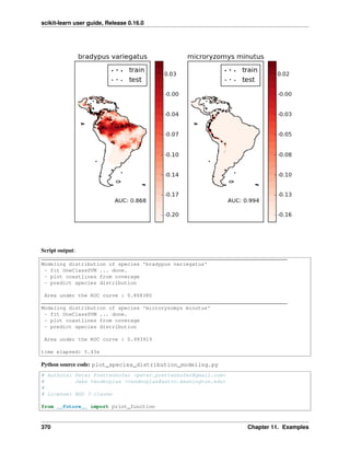
![scikit-learn user guide, Release 0.16.0
from time import time
import numpy as np
import matplotlib.pyplot as plt
from sklearn.datasets.base import Bunch
from sklearn.datasets import fetch_species_distributions
from sklearn.datasets.species_distributions import construct_grids
from sklearn import svm, metrics
# if basemap is available, we'll use it.
# otherwise, we'll improvise later...
try:
from mpl_toolkits.basemap import Basemap
basemap = True
except ImportError:
basemap = False
print(__doc__)
def create_species_bunch(species_name, train, test, coverages, xgrid, ygrid):
"""Create a bunch with information about a particular organism
This will use the test/train record arrays to extract the
data specific to the given species name.
"""
bunch = Bunch(name=' '.join(species_name.split("_")[:2]))
species_name = species_name.encode('ascii')
points = dict(test=test, train=train)
for label, pts in points.items():
# choose points associated with the desired species
pts = pts[pts['species'] == species_name]
bunch['pts_%s' % label] = pts
# determine coverage values for each of the training & testing points
ix = np.searchsorted(xgrid, pts['dd long'])
iy = np.searchsorted(ygrid, pts['dd lat'])
bunch['cov_%s' % label] = coverages[:, -iy, ix].T
return bunch
def plot_species_distribution(species=("bradypus_variegatus_0",
"microryzomys_minutus_0")):
"""
Plot the species distribution.
"""
if len(species) > 2:
print("Note: when more than two species are provided,"
" only the first two will be used")
t0 = time()
# Load the compressed data
data = fetch_species_distributions()
11.2. Examples based on real world datasets 371](https://image.slidesharecdn.com/scikit-learn0-150409112902-conversion-gate01/85/Scikit-learn-0-16-0-user-guide-381-320.jpg)
![scikit-learn user guide, Release 0.16.0
# Set up the data grid
xgrid, ygrid = construct_grids(data)
# The grid in x,y coordinates
X, Y = np.meshgrid(xgrid, ygrid[::-1])
# create a bunch for each species
BV_bunch = create_species_bunch(species[0],
data.train, data.test,
data.coverages, xgrid, ygrid)
MM_bunch = create_species_bunch(species[1],
data.train, data.test,
data.coverages, xgrid, ygrid)
# background points (grid coordinates) for evaluation
np.random.seed(13)
background_points = np.c_[np.random.randint(low=0, high=data.Ny,
size=10000),
np.random.randint(low=0, high=data.Nx,
size=10000)].T
# We'll make use of the fact that coverages[6] has measurements at all
# land points. This will help us decide between land and water.
land_reference = data.coverages[6]
# Fit, predict, and plot for each species.
for i, species in enumerate([BV_bunch, MM_bunch]):
print("_" * 80)
print("Modeling distribution of species '%s'" % species.name)
# Standardize features
mean = species.cov_train.mean(axis=0)
std = species.cov_train.std(axis=0)
train_cover_std = (species.cov_train - mean) / std
# Fit OneClassSVM
print(" - fit OneClassSVM ... ", end='')
clf = svm.OneClassSVM(nu=0.1, kernel="rbf", gamma=0.5)
clf.fit(train_cover_std)
print("done.")
# Plot map of South America
plt.subplot(1, 2, i + 1)
if basemap:
print(" - plot coastlines using basemap")
m = Basemap(projection='cyl', llcrnrlat=Y.min(),
urcrnrlat=Y.max(), llcrnrlon=X.min(),
urcrnrlon=X.max(), resolution='c')
m.drawcoastlines()
m.drawcountries()
else:
print(" - plot coastlines from coverage")
plt.contour(X, Y, land_reference,
levels=[-9999], colors="k",
linestyles="solid")
plt.xticks([])
plt.yticks([])
372 Chapter 11. Examples](https://image.slidesharecdn.com/scikit-learn0-150409112902-conversion-gate01/85/Scikit-learn-0-16-0-user-guide-382-320.jpg)
![scikit-learn user guide, Release 0.16.0
print(" - predict species distribution")
# Predict species distribution using the training data
Z = np.ones((data.Ny, data.Nx), dtype=np.float64)
# We'll predict only for the land points.
idx = np.where(land_reference > -9999)
coverages_land = data.coverages[:, idx[0], idx[1]].T
pred = clf.decision_function((coverages_land - mean) / std)[:, 0]
Z *= pred.min()
Z[idx[0], idx[1]] = pred
levels = np.linspace(Z.min(), Z.max(), 25)
Z[land_reference == -9999] = -9999
# plot contours of the prediction
plt.contourf(X, Y, Z, levels=levels, cmap=plt.cm.Reds)
plt.colorbar(format='%.2f')
# scatter training/testing points
plt.scatter(species.pts_train['dd long'], species.pts_train['dd lat'],
s=2 ** 2, c='black',
marker='^', label='train')
plt.scatter(species.pts_test['dd long'], species.pts_test['dd lat'],
s=2 ** 2, c='black',
marker='x', label='test')
plt.legend()
plt.title(species.name)
plt.axis('equal')
# Compute AUC with regards to background points
pred_background = Z[background_points[0], background_points[1]]
pred_test = clf.decision_function((species.cov_test - mean)
/ std)[:, 0]
scores = np.r_[pred_test, pred_background]
y = np.r_[np.ones(pred_test.shape), np.zeros(pred_background.shape)]
fpr, tpr, thresholds = metrics.roc_curve(y, scores)
roc_auc = metrics.auc(fpr, tpr)
plt.text(-35, -70, "AUC: %.3f" % roc_auc, ha="right")
print("n Area under the ROC curve : %f" % roc_auc)
print("ntime elapsed: %.2fs" % (time() - t0))
plot_species_distribution()
plt.show()
Total running time of the example: 5.44 seconds ( 0 minutes 5.44 seconds)
11.2.7 Visualizing the stock market structure
This example employs several unsupervised learning techniques to extract the stock market structure from variations
in historical quotes.
The quantity that we use is the daily variation in quote price: quotes that are linked tend to cofluctuate during a day.
11.2. Examples based on real world datasets 373](https://image.slidesharecdn.com/scikit-learn0-150409112902-conversion-gate01/85/Scikit-learn-0-16-0-user-guide-383-320.jpg)

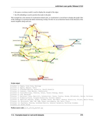
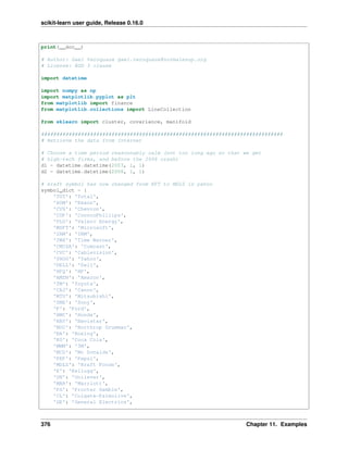
![scikit-learn user guide, Release 0.16.0
'WFC': 'Wells Fargo',
'JPM': 'JPMorgan Chase',
'AIG': 'AIG',
'AXP': 'American express',
'BAC': 'Bank of America',
'GS': 'Goldman Sachs',
'AAPL': 'Apple',
'SAP': 'SAP',
'CSCO': 'Cisco',
'TXN': 'Texas instruments',
'XRX': 'Xerox',
'LMT': 'Lookheed Martin',
'WMT': 'Wal-Mart',
'WBA': 'Walgreen',
'HD': 'Home Depot',
'GSK': 'GlaxoSmithKline',
'PFE': 'Pfizer',
'SNY': 'Sanofi-Aventis',
'NVS': 'Novartis',
'KMB': 'Kimberly-Clark',
'R': 'Ryder',
'GD': 'General Dynamics',
'RTN': 'Raytheon',
'CVS': 'CVS',
'CAT': 'Caterpillar',
'DD': 'DuPont de Nemours'}
symbols, names = np.array(list(symbol_dict.items())).T
quotes = [finance.quotes_historical_yahoo(symbol, d1, d2, asobject=True)
for symbol in symbols]
open = np.array([q.open for q in quotes]).astype(np.float)
close = np.array([q.close for q in quotes]).astype(np.float)
# The daily variations of the quotes are what carry most information
variation = close - open
###############################################################################
# Learn a graphical structure from the correlations
edge_model = covariance.GraphLassoCV()
# standardize the time series: using correlations rather than covariance
# is more efficient for structure recovery
X = variation.copy().T
X /= X.std(axis=0)
edge_model.fit(X)
###############################################################################
# Cluster using affinity propagation
_, labels = cluster.affinity_propagation(edge_model.covariance_)
n_labels = labels.max()
for i in range(n_labels + 1):
print('Cluster %i: %s' % ((i + 1), ', '.join(names[labels == i])))
###############################################################################
11.2. Examples based on real world datasets 377](https://image.slidesharecdn.com/scikit-learn0-150409112902-conversion-gate01/85/Scikit-learn-0-16-0-user-guide-387-320.jpg)
![scikit-learn user guide, Release 0.16.0
# Find a low-dimension embedding for visualization: find the best position of
# the nodes (the stocks) on a 2D plane
# We use a dense eigen_solver to achieve reproducibility (arpack is
# initiated with random vectors that we don't control). In addition, we
# use a large number of neighbors to capture the large-scale structure.
node_position_model = manifold.LocallyLinearEmbedding(
n_components=2, eigen_solver='dense', n_neighbors=6)
embedding = node_position_model.fit_transform(X.T).T
###############################################################################
# Visualization
plt.figure(1, facecolor='w', figsize=(10, 8))
plt.clf()
ax = plt.axes([0., 0., 1., 1.])
plt.axis('off')
# Display a graph of the partial correlations
partial_correlations = edge_model.precision_.copy()
d = 1 / np.sqrt(np.diag(partial_correlations))
partial_correlations *= d
partial_correlations *= d[:, np.newaxis]
non_zero = (np.abs(np.triu(partial_correlations, k=1)) > 0.02)
# Plot the nodes using the coordinates of our embedding
plt.scatter(embedding[0], embedding[1], s=100 * d ** 2, c=labels,
cmap=plt.cm.spectral)
# Plot the edges
start_idx, end_idx = np.where(non_zero)
#a sequence of (*line0*, *line1*, *line2*), where::
# linen = (x0, y0), (x1, y1), ... (xm, ym)
segments = [[embedding[:, start], embedding[:, stop]]
for start, stop in zip(start_idx, end_idx)]
values = np.abs(partial_correlations[non_zero])
lc = LineCollection(segments,
zorder=0, cmap=plt.cm.hot_r,
norm=plt.Normalize(0, .7 * values.max()))
lc.set_array(values)
lc.set_linewidths(15 * values)
ax.add_collection(lc)
# Add a label to each node. The challenge here is that we want to
# position the labels to avoid overlap with other labels
for index, (name, label, (x, y)) in enumerate(
zip(names, labels, embedding.T)):
dx = x - embedding[0]
dx[index] = 1
dy = y - embedding[1]
dy[index] = 1
this_dx = dx[np.argmin(np.abs(dy))]
this_dy = dy[np.argmin(np.abs(dx))]
if this_dx > 0:
horizontalalignment = 'left'
x = x + .002
else:
378 Chapter 11. Examples](https://image.slidesharecdn.com/scikit-learn0-150409112902-conversion-gate01/85/Scikit-learn-0-16-0-user-guide-388-320.jpg)
![scikit-learn user guide, Release 0.16.0
horizontalalignment = 'right'
x = x - .002
if this_dy > 0:
verticalalignment = 'bottom'
y = y + .002
else:
verticalalignment = 'top'
y = y - .002
plt.text(x, y, name, size=10,
horizontalalignment=horizontalalignment,
verticalalignment=verticalalignment,
bbox=dict(facecolor='w',
edgecolor=plt.cm.spectral(label / float(n_labels)),
alpha=.6))
plt.xlim(embedding[0].min() - .15 * embedding[0].ptp(),
embedding[0].max() + .10 * embedding[0].ptp(),)
plt.ylim(embedding[1].min() - .03 * embedding[1].ptp(),
embedding[1].max() + .03 * embedding[1].ptp())
plt.show()
Total running time of the example: 4.14 seconds ( 0 minutes 4.14 seconds)
Fig. 11.19: Wikipedia principal eigenvector
11.2.8 Wikipedia principal eigenvector
A classical way to assert the relative importance of vertices in a graph is to compute the principal eigenvector of the
adjacency matrix so as to assign to each vertex the values of the components of the first eigenvector as a centrality
score:
http://en.wikipedia.org/wiki/Eigenvector_centrality
On the graph of webpages and links those values are called the PageRank scores by Google.
The goal of this example is to analyze the graph of links inside wikipedia articles to rank articles by relative importance
according to this eigenvector centrality.
The traditional way to compute the principal eigenvector is to use the power iteration method:
http://en.wikipedia.org/wiki/Power_iteration
Here the computation is achieved thanks to Martinsson’s Randomized SVD algorithm implemented in the scikit.
11.2. Examples based on real world datasets 379](https://image.slidesharecdn.com/scikit-learn0-150409112902-conversion-gate01/85/Scikit-learn-0-16-0-user-guide-389-320.jpg)
![scikit-learn user guide, Release 0.16.0
The graph data is fetched from the DBpedia dumps. DBpedia is an extraction of the latent structured data of the
Wikipedia content.
Python source code: wikipedia_principal_eigenvector.py
# Author: Olivier Grisel <olivier.grisel@ensta.org>
# License: BSD 3 clause
from __future__ import print_function
from bz2 import BZ2File
import os
from datetime import datetime
from pprint import pprint
from time import time
import numpy as np
from scipy import sparse
from sklearn.decomposition import randomized_svd
from sklearn.externals.joblib import Memory
print(__doc__)
###############################################################################
# Where to download the data, if not already on disk
redirects_url = "http://downloads.dbpedia.org/3.5.1/en/redirects_en.nt.bz2"
redirects_filename = redirects_url.rsplit("/", 1)[1]
page_links_url = "http://downloads.dbpedia.org/3.5.1/en/page_links_en.nt.bz2"
page_links_filename = page_links_url.rsplit("/", 1)[1]
resources = [
(redirects_url, redirects_filename),
(page_links_url, page_links_filename),
]
for url, filename in resources:
if not os.path.exists(filename):
import urllib
print("Downloading data from '%s', please wait..." % url)
opener = urllib.urlopen(url)
open(filename, 'wb').write(opener.read())
print()
###############################################################################
# Loading the redirect files
memory = Memory(cachedir=".")
def index(redirects, index_map, k):
"""Find the index of an article name after redirect resolution"""
k = redirects.get(k, k)
return index_map.setdefault(k, len(index_map))
380 Chapter 11. Examples](https://image.slidesharecdn.com/scikit-learn0-150409112902-conversion-gate01/85/Scikit-learn-0-16-0-user-guide-390-320.jpg)
![scikit-learn user guide, Release 0.16.0
DBPEDIA_RESOURCE_PREFIX_LEN = len("http://dbpedia.org/resource/")
SHORTNAME_SLICE = slice(DBPEDIA_RESOURCE_PREFIX_LEN + 1, -1)
def short_name(nt_uri):
"""Remove the < and > URI markers and the common URI prefix"""
return nt_uri[SHORTNAME_SLICE]
def get_redirects(redirects_filename):
"""Parse the redirections and build a transitively closed map out of it"""
redirects = {}
print("Parsing the NT redirect file")
for l, line in enumerate(BZ2File(redirects_filename)):
split = line.split()
if len(split) != 4:
print("ignoring malformed line: " + line)
continue
redirects[short_name(split[0])] = short_name(split[2])
if l % 1000000 == 0:
print("[%s] line: %08d" % (datetime.now().isoformat(), l))
# compute the transitive closure
print("Computing the transitive closure of the redirect relation")
for l, source in enumerate(redirects.keys()):
transitive_target = None
target = redirects[source]
seen = set([source])
while True:
transitive_target = target
target = redirects.get(target)
if target is None or target in seen:
break
seen.add(target)
redirects[source] = transitive_target
if l % 1000000 == 0:
print("[%s] line: %08d" % (datetime.now().isoformat(), l))
return redirects
# disabling joblib as the pickling of large dicts seems much too slow
#@memory.cache
def get_adjacency_matrix(redirects_filename, page_links_filename, limit=None):
"""Extract the adjacency graph as a scipy sparse matrix
Redirects are resolved first.
Returns X, the scipy sparse adjacency matrix, redirects as python
dict from article names to article names and index_map a python dict
from article names to python int (article indexes).
"""
print("Computing the redirect map")
redirects = get_redirects(redirects_filename)
print("Computing the integer index map")
index_map = dict()
11.2. Examples based on real world datasets 381](https://image.slidesharecdn.com/scikit-learn0-150409112902-conversion-gate01/85/Scikit-learn-0-16-0-user-guide-391-320.jpg)
![scikit-learn user guide, Release 0.16.0
links = list()
for l, line in enumerate(BZ2File(page_links_filename)):
split = line.split()
if len(split) != 4:
print("ignoring malformed line: " + line)
continue
i = index(redirects, index_map, short_name(split[0]))
j = index(redirects, index_map, short_name(split[2]))
links.append((i, j))
if l % 1000000 == 0:
print("[%s] line: %08d" % (datetime.now().isoformat(), l))
if limit is not None and l >= limit - 1:
break
print("Computing the adjacency matrix")
X = sparse.lil_matrix((len(index_map), len(index_map)), dtype=np.float32)
for i, j in links:
X[i, j] = 1.0
del links
print("Converting to CSR representation")
X = X.tocsr()
print("CSR conversion done")
return X, redirects, index_map
# stop after 5M links to make it possible to work in RAM
X, redirects, index_map = get_adjacency_matrix(
redirects_filename, page_links_filename, limit=5000000)
names = dict((i, name) for name, i in index_map.iteritems())
print("Computing the principal singular vectors using randomized_svd")
t0 = time()
U, s, V = randomized_svd(X, 5, n_iter=3)
print("done in %0.3fs" % (time() - t0))
# print the names of the wikipedia related strongest compenents of the the
# principal singular vector which should be similar to the highest eigenvector
print("Top wikipedia pages according to principal singular vectors")
pprint([names[i] for i in np.abs(U.T[0]).argsort()[-10:]])
pprint([names[i] for i in np.abs(V[0]).argsort()[-10:]])
def centrality_scores(X, alpha=0.85, max_iter=100, tol=1e-10):
"""Power iteration computation of the principal eigenvector
This method is also known as Google PageRank and the implementation
is based on the one from the NetworkX project (BSD licensed too)
with copyrights by:
Aric Hagberg <hagberg@lanl.gov>
Dan Schult <dschult@colgate.edu>
Pieter Swart <swart@lanl.gov>
"""
n = X.shape[0]
X = X.copy()
incoming_counts = np.asarray(X.sum(axis=1)).ravel()
382 Chapter 11. Examples](https://image.slidesharecdn.com/scikit-learn0-150409112902-conversion-gate01/85/Scikit-learn-0-16-0-user-guide-392-320.jpg)
![scikit-learn user guide, Release 0.16.0
print("Normalizing the graph")
for i in incoming_counts.nonzero()[0]:
X.data[X.indptr[i]:X.indptr[i + 1]] *= 1.0 / incoming_counts[i]
dangle = np.asarray(np.where(X.sum(axis=1) == 0, 1.0 / n, 0)).ravel()
scores = np.ones(n, dtype=np.float32) / n # initial guess
for i in range(max_iter):
print("power iteration #%d" % i)
prev_scores = scores
scores = (alpha * (scores * X + np.dot(dangle, prev_scores))
+ (1 - alpha) * prev_scores.sum() / n)
# check convergence: normalized l_inf norm
scores_max = np.abs(scores).max()
if scores_max == 0.0:
scores_max = 1.0
err = np.abs(scores - prev_scores).max() / scores_max
print("error: %0.6f" % err)
if err < n * tol:
return scores
return scores
print("Computing principal eigenvector score using a power iteration method")
t0 = time()
scores = centrality_scores(X, max_iter=100, tol=1e-10)
print("done in %0.3fs" % (time() - t0))
pprint([names[i] for i in np.abs(scores).argsort()[-10:]])
Fig. 11.20: Prediction Latency
11.2. Examples based on real world datasets 383](https://image.slidesharecdn.com/scikit-learn0-150409112902-conversion-gate01/85/Scikit-learn-0-16-0-user-guide-393-320.jpg)

![scikit-learn user guide, Release 0.16.0
Benchmarking SGDRegressor(alpha=0.01, average=False, epsilon=0.1, eta0=0.01,
fit_intercept=True, l1_ratio=0.25, learning_rate='invscaling',
loss='squared_loss', n_iter=5, penalty='elasticnet', power_t=0.25,
random_state=None, shuffle=True, verbose=0, warm_start=False)
Benchmarking RandomForestRegressor(bootstrap=True, criterion='mse', max_depth=None,
max_features='auto', max_leaf_nodes=None, min_samples_leaf=1,
min_samples_split=2, min_weight_fraction_leaf=0.0,
n_estimators=10, n_jobs=1, oob_score=False, random_state=None,
verbose=0, warm_start=False)
Benchmarking SVR(C=1.0, cache_size=200, coef0=0.0, degree=3, epsilon=0.1, gamma=0.0,
kernel='rbf', max_iter=-1, shrinking=True, tol=0.001, verbose=False)
benchmarking with 100 features
benchmarking with 250 features
benchmarking with 500 features
example run in 6.37s
Python source code: plot_prediction_latency.py
# Authors: Eustache Diemert <eustache@diemert.fr>
# License: BSD 3 clause
from __future__ import print_function
from collections import defaultdict
import time
import gc
import numpy as np
import matplotlib.pyplot as plt
from scipy.stats import scoreatpercentile
from sklearn.datasets.samples_generator import make_regression
from sklearn.ensemble.forest import RandomForestRegressor
from sklearn.linear_model.ridge import Ridge
from sklearn.linear_model.stochastic_gradient import SGDRegressor
from sklearn.svm.classes import SVR
def _not_in_sphinx():
# Hack to detect whether we are running by the sphinx builder
return '__file__' in globals()
def atomic_benchmark_estimator(estimator, X_test, verbose=False):
"""Measure runtime prediction of each instance."""
n_instances = X_test.shape[0]
runtimes = np.zeros(n_instances, dtype=np.float)
for i in range(n_instances):
instance = X_test[i, :]
start = time.time()
estimator.predict(instance)
runtimes[i] = time.time() - start
if verbose:
print("atomic_benchmark runtimes:", min(runtimes), scoreatpercentile(
runtimes, 50), max(runtimes))
return runtimes
def bulk_benchmark_estimator(estimator, X_test, n_bulk_repeats, verbose):
11.2. Examples based on real world datasets 385](https://image.slidesharecdn.com/scikit-learn0-150409112902-conversion-gate01/85/Scikit-learn-0-16-0-user-guide-395-320.jpg)
![scikit-learn user guide, Release 0.16.0
"""Measure runtime prediction of the whole input."""
n_instances = X_test.shape[0]
runtimes = np.zeros(n_bulk_repeats, dtype=np.float)
for i in range(n_bulk_repeats):
start = time.time()
estimator.predict(X_test)
runtimes[i] = time.time() - start
runtimes = np.array(list(map(lambda x: x / float(n_instances), runtimes)))
if verbose:
print("bulk_benchmark runtimes:", min(runtimes), scoreatpercentile(
runtimes, 50), max(runtimes))
return runtimes
def benchmark_estimator(estimator, X_test, n_bulk_repeats=30, verbose=False):
"""
Measure runtimes of prediction in both atomic and bulk mode.
Parameters
----------
estimator : already trained estimator supporting `predict()`
X_test : test input
n_bulk_repeats : how many times to repeat when evaluating bulk mode
Returns
-------
atomic_runtimes, bulk_runtimes : a pair of `np.array` which contain the
runtimes in seconds.
"""
atomic_runtimes = atomic_benchmark_estimator(estimator, X_test, verbose)
bulk_runtimes = bulk_benchmark_estimator(estimator, X_test, n_bulk_repeats,
verbose)
return atomic_runtimes, bulk_runtimes
def generate_dataset(n_train, n_test, n_features, noise=0.1, verbose=False):
"""Generate a regression dataset with the given parameters."""
if verbose:
print("generating dataset...")
X, y, coef = make_regression(n_samples=n_train + n_test,
n_features=n_features, noise=noise, coef=True)
X_train = X[:n_train]
y_train = y[:n_train]
X_test = X[n_train:]
y_test = y[n_train:]
idx = np.arange(n_train)
np.random.seed(13)
np.random.shuffle(idx)
X_train = X_train[idx]
y_train = y_train[idx]
std = X_train.std(axis=0)
mean = X_train.mean(axis=0)
X_train = (X_train - mean) / std
X_test = (X_test - mean) / std
std = y_train.std(axis=0)
386 Chapter 11. Examples](https://image.slidesharecdn.com/scikit-learn0-150409112902-conversion-gate01/85/Scikit-learn-0-16-0-user-guide-396-320.jpg)
![scikit-learn user guide, Release 0.16.0
mean = y_train.mean(axis=0)
y_train = (y_train - mean) / std
y_test = (y_test - mean) / std
gc.collect()
if verbose:
print("ok")
return X_train, y_train, X_test, y_test
def boxplot_runtimes(runtimes, pred_type, configuration):
"""
Plot a new `Figure` with boxplots of prediction runtimes.
Parameters
----------
runtimes : list of `np.array` of latencies in micro-seconds
cls_names : list of estimator class names that generated the runtimes
pred_type : 'bulk' or 'atomic'
"""
fig, ax1 = plt.subplots(figsize=(10, 6))
bp = plt.boxplot(runtimes, )
cls_infos = ['%sn(%d %s)' % (estimator_conf['name'],
estimator_conf['complexity_computer'](
estimator_conf['instance']),
estimator_conf['complexity_label']) for
estimator_conf in configuration['estimators']]
plt.setp(ax1, xticklabels=cls_infos)
plt.setp(bp['boxes'], color='black')
plt.setp(bp['whiskers'], color='black')
plt.setp(bp['fliers'], color='red', marker='+')
ax1.yaxis.grid(True, linestyle='-', which='major', color='lightgrey',
alpha=0.5)
ax1.set_axisbelow(True)
ax1.set_title('Prediction Time per Instance - %s, %d feats.' % (
pred_type.capitalize(),
configuration['n_features']))
ax1.set_ylabel('Prediction Time (us)')
plt.show()
def benchmark(configuration):
"""Run the whole benchmark."""
X_train, y_train, X_test, y_test = generate_dataset(
configuration['n_train'], configuration['n_test'],
configuration['n_features'])
stats = {}
for estimator_conf in configuration['estimators']:
print("Benchmarking", estimator_conf['instance'])
estimator_conf['instance'].fit(X_train, y_train)
gc.collect()
11.2. Examples based on real world datasets 387](https://image.slidesharecdn.com/scikit-learn0-150409112902-conversion-gate01/85/Scikit-learn-0-16-0-user-guide-397-320.jpg)
![scikit-learn user guide, Release 0.16.0
a, b = benchmark_estimator(estimator_conf['instance'], X_test)
stats[estimator_conf['name']] = {'atomic': a, 'bulk': b}
cls_names = [estimator_conf['name'] for estimator_conf in configuration[
'estimators']]
runtimes = [1e6 * stats[clf_name]['atomic'] for clf_name in cls_names]
boxplot_runtimes(runtimes, 'atomic', configuration)
runtimes = [1e6 * stats[clf_name]['bulk'] for clf_name in cls_names]
boxplot_runtimes(runtimes, 'bulk (%d)' % configuration['n_test'],
configuration)
def n_feature_influence(estimators, n_train, n_test, n_features, percentile):
"""
Estimate influence of the number of features on prediction time.
Parameters
----------
estimators : dict of (name (str), estimator) to benchmark
n_train : nber of training instances (int)
n_test : nber of testing instances (int)
n_features : list of feature-space dimensionality to test (int)
percentile : percentile at which to measure the speed (int [0-100])
Returns:
--------
percentiles : dict(estimator_name,
dict(n_features, percentile_perf_in_us))
"""
percentiles = defaultdict(defaultdict)
for n in n_features:
print("benchmarking with %d features" % n)
X_train, y_train, X_test, y_test = generate_dataset(n_train, n_test, n)
for cls_name, estimator in estimators.items():
estimator.fit(X_train, y_train)
gc.collect()
runtimes = bulk_benchmark_estimator(estimator, X_test, 30, False)
percentiles[cls_name][n] = 1e6 * scoreatpercentile(runtimes,
percentile)
return percentiles
def plot_n_features_influence(percentiles, percentile):
fig, ax1 = plt.subplots(figsize=(10, 6))
colors = ['r', 'g', 'b']
for i, cls_name in enumerate(percentiles.keys()):
x = np.array(sorted([n for n in percentiles[cls_name].keys()]))
y = np.array([percentiles[cls_name][n] for n in x])
plt.plot(x, y, color=colors[i], )
ax1.yaxis.grid(True, linestyle='-', which='major', color='lightgrey',
alpha=0.5)
ax1.set_axisbelow(True)
ax1.set_title('Evolution of Prediction Time with #Features')
ax1.set_xlabel('#Features')
ax1.set_ylabel('Prediction Time at %d%%-ile (us)' % percentile)
388 Chapter 11. Examples](https://image.slidesharecdn.com/scikit-learn0-150409112902-conversion-gate01/85/Scikit-learn-0-16-0-user-guide-398-320.jpg)
![scikit-learn user guide, Release 0.16.0
plt.show()
def benchmark_throughputs(configuration, duration_secs=0.1):
"""benchmark throughput for different estimators."""
X_train, y_train, X_test, y_test = generate_dataset(
configuration['n_train'], configuration['n_test'],
configuration['n_features'])
throughputs = dict()
for estimator_config in configuration['estimators']:
estimator_config['instance'].fit(X_train, y_train)
start_time = time.time()
n_predictions = 0
while (time.time() - start_time) < duration_secs:
estimator_config['instance'].predict(X_test[0])
n_predictions += 1
throughputs[estimator_config['name']] = n_predictions / duration_secs
return throughputs
def plot_benchmark_throughput(throughputs, configuration):
fig, ax = plt.subplots(figsize=(10, 6))
colors = ['r', 'g', 'b']
cls_infos = ['%sn(%d %s)' % (estimator_conf['name'],
estimator_conf['complexity_computer'](
estimator_conf['instance']),
estimator_conf['complexity_label']) for
estimator_conf in configuration['estimators']]
cls_values = [throughputs[estimator_conf['name']] for estimator_conf in
configuration['estimators']]
plt.bar(range(len(throughputs)), cls_values, width=0.5, color=colors)
ax.set_xticks(np.linspace(0.25, len(throughputs) - 0.75, len(throughputs)))
ax.set_xticklabels(cls_infos, fontsize=10)
ymax = max(cls_values) * 1.2
ax.set_ylim((0, ymax))
ax.set_ylabel('Throughput (predictions/sec)')
ax.set_title('Prediction Throughput for different estimators (%d '
'features)' % configuration['n_features'])
plt.show()
###############################################################################
# main code
start_time = time.time()
# benchmark bulk/atomic prediction speed for various regressors
configuration = {
'n_train': int(1e3),
'n_test': int(1e2),
'n_features': int(1e2),
'estimators': [
{'name': 'Linear Model',
'instance': SGDRegressor(penalty='elasticnet', alpha=0.01,
l1_ratio=0.25, fit_intercept=True),
'complexity_label': 'non-zero coefficients',
'complexity_computer': lambda clf: np.count_nonzero(clf.coef_)},
{'name': 'RandomForest',
11.2. Examples based on real world datasets 389](https://image.slidesharecdn.com/scikit-learn0-150409112902-conversion-gate01/85/Scikit-learn-0-16-0-user-guide-399-320.jpg)
![scikit-learn user guide, Release 0.16.0
'instance': RandomForestRegressor(),
'complexity_label': 'estimators',
'complexity_computer': lambda clf: clf.n_estimators},
{'name': 'SVR',
'instance': SVR(kernel='rbf'),
'complexity_label': 'support vectors',
'complexity_computer': lambda clf: len(clf.support_vectors_)},
]
}
benchmark(configuration)
# benchmark n_features influence on prediction speed
percentile = 90
percentiles = n_feature_influence({'ridge': Ridge()},
configuration['n_train'],
configuration['n_test'],
[100, 250, 500], percentile)
plot_n_features_influence(percentiles, percentile)
# benchmark throughput
throughputs = benchmark_throughputs(configuration)
plot_benchmark_throughput(throughputs, configuration)
stop_time = time.time()
print("example run in %.2fs" % (stop_time - start_time))
Total running time of the example: 6.37 seconds ( 0 minutes 6.37 seconds)
Fig. 11.21: Libsvm GUI
11.2.10 Libsvm GUI
A simple graphical frontend for Libsvm mainly intended for didactic purposes. You can create data points by point
and click and visualize the decision region induced by different kernels and parameter settings.
To create positive examples click the left mouse button; to create negative examples click the right button.
If all examples are from the same class, it uses a one-class SVM.
Python source code: svm_gui.py
from __future__ import division, print_function
390 Chapter 11. Examples](https://image.slidesharecdn.com/scikit-learn0-150409112902-conversion-gate01/85/Scikit-learn-0-16-0-user-guide-400-320.jpg)
![scikit-learn user guide, Release 0.16.0
print(__doc__)
# Author: Peter Prettenhoer <peter.prettenhofer@gmail.com>
#
# License: BSD 3 clause
import matplotlib
matplotlib.use('TkAgg')
from matplotlib.backends.backend_tkagg import FigureCanvasTkAgg
from matplotlib.backends.backend_tkagg import NavigationToolbar2TkAgg
from matplotlib.figure import Figure
from matplotlib.contour import ContourSet
import Tkinter as Tk
import sys
import numpy as np
from sklearn import svm
from sklearn.datasets import dump_svmlight_file
from sklearn.externals.six.moves import xrange
y_min, y_max = -50, 50
x_min, x_max = -50, 50
class Model(object):
"""The Model which hold the data. It implements the
observable in the observer pattern and notifies the
registered observers on change event.
"""
def __init__(self):
self.observers = []
self.surface = None
self.data = []
self.cls = None
self.surface_type = 0
def changed(self, event):
"""Notify the observers. """
for observer in self.observers:
observer.update(event, self)
def add_observer(self, observer):
"""Register an observer. """
self.observers.append(observer)
def set_surface(self, surface):
self.surface = surface
def dump_svmlight_file(self, file):
data = np.array(self.data)
X = data[:, 0:2]
y = data[:, 2]
dump_svmlight_file(X, y, file)
11.2. Examples based on real world datasets 391](https://image.slidesharecdn.com/scikit-learn0-150409112902-conversion-gate01/85/Scikit-learn-0-16-0-user-guide-401-320.jpg)
![scikit-learn user guide, Release 0.16.0
class Controller(object):
def __init__(self, model):
self.model = model
self.kernel = Tk.IntVar()
self.surface_type = Tk.IntVar()
# Whether or not a model has been fitted
self.fitted = False
def fit(self):
print("fit the model")
train = np.array(self.model.data)
X = train[:, 0:2]
y = train[:, 2]
C = float(self.complexity.get())
gamma = float(self.gamma.get())
coef0 = float(self.coef0.get())
degree = int(self.degree.get())
kernel_map = {0: "linear", 1: "rbf", 2: "poly"}
if len(np.unique(y)) == 1:
clf = svm.OneClassSVM(kernel=kernel_map[self.kernel.get()],
gamma=gamma, coef0=coef0, degree=degree)
clf.fit(X)
else:
clf = svm.SVC(kernel=kernel_map[self.kernel.get()], C=C,
gamma=gamma, coef0=coef0, degree=degree)
clf.fit(X, y)
if hasattr(clf, 'score'):
print("Accuracy:", clf.score(X, y) * 100)
X1, X2, Z = self.decision_surface(clf)
self.model.clf = clf
self.model.set_surface((X1, X2, Z))
self.model.surface_type = self.surface_type.get()
self.fitted = True
self.model.changed("surface")
def decision_surface(self, cls):
delta = 1
x = np.arange(x_min, x_max + delta, delta)
y = np.arange(y_min, y_max + delta, delta)
X1, X2 = np.meshgrid(x, y)
Z = cls.decision_function(np.c_[X1.ravel(), X2.ravel()])
Z = Z.reshape(X1.shape)
return X1, X2, Z
def clear_data(self):
self.model.data = []
self.fitted = False
self.model.changed("clear")
def add_example(self, x, y, label):
self.model.data.append((x, y, label))
self.model.changed("example_added")
# update decision surface if already fitted.
self.refit()
def refit(self):
392 Chapter 11. Examples](https://image.slidesharecdn.com/scikit-learn0-150409112902-conversion-gate01/85/Scikit-learn-0-16-0-user-guide-402-320.jpg)
![scikit-learn user guide, Release 0.16.0
"""Refit the model if already fitted. """
if self.fitted:
self.fit()
class View(object):
"""Test docstring. """
def __init__(self, root, controller):
f = Figure()
ax = f.add_subplot(111)
ax.set_xticks([])
ax.set_yticks([])
ax.set_xlim((x_min, x_max))
ax.set_ylim((y_min, y_max))
canvas = FigureCanvasTkAgg(f, master=root)
canvas.show()
canvas.get_tk_widget().pack(side=Tk.TOP, fill=Tk.BOTH, expand=1)
canvas._tkcanvas.pack(side=Tk.TOP, fill=Tk.BOTH, expand=1)
canvas.mpl_connect('button_press_event', self.onclick)
toolbar = NavigationToolbar2TkAgg(canvas, root)
toolbar.update()
self.controllbar = ControllBar(root, controller)
self.f = f
self.ax = ax
self.canvas = canvas
self.controller = controller
self.contours = []
self.c_labels = None
self.plot_kernels()
def plot_kernels(self):
self.ax.text(-50, -60, "Linear: $u^T v$")
self.ax.text(-20, -60, "RBF: $exp (-gamma | u-v |^2)$")
self.ax.text(10, -60, "Poly: $(gamma , u^T v + r)^d$")
def onclick(self, event):
if event.xdata and event.ydata:
if event.button == 1:
self.controller.add_example(event.xdata, event.ydata, 1)
elif event.button == 3:
self.controller.add_example(event.xdata, event.ydata, -1)
def update_example(self, model, idx):
x, y, l = model.data[idx]
if l == 1:
color = 'w'
elif l == -1:
color = 'k'
self.ax.plot([x], [y], "%so" % color, scalex=0.0, scaley=0.0)
def update(self, event, model):
if event == "examples_loaded":
for i in xrange(len(model.data)):
self.update_example(model, i)
if event == "example_added":
self.update_example(model, -1)
11.2. Examples based on real world datasets 393](https://image.slidesharecdn.com/scikit-learn0-150409112902-conversion-gate01/85/Scikit-learn-0-16-0-user-guide-403-320.jpg)
![scikit-learn user guide, Release 0.16.0
if event == "clear":
self.ax.clear()
self.ax.set_xticks([])
self.ax.set_yticks([])
self.contours = []
self.c_labels = None
self.plot_kernels()
if event == "surface":
self.remove_surface()
self.plot_support_vectors(model.clf.support_vectors_)
self.plot_decision_surface(model.surface, model.surface_type)
self.canvas.draw()
def remove_surface(self):
"""Remove old decision surface."""
if len(self.contours) > 0:
for contour in self.contours:
if isinstance(contour, ContourSet):
for lineset in contour.collections:
lineset.remove()
else:
contour.remove()
self.contours = []
def plot_support_vectors(self, support_vectors):
"""Plot the support vectors by placing circles over the
corresponding data points and adds the circle collection
to the contours list."""
cs = self.ax.scatter(support_vectors[:, 0], support_vectors[:, 1],
s=80, edgecolors="k", facecolors="none")
self.contours.append(cs)
def plot_decision_surface(self, surface, type):
X1, X2, Z = surface
if type == 0:
levels = [-1.0, 0.0, 1.0]
linestyles = ['dashed', 'solid', 'dashed']
colors = 'k'
self.contours.append(self.ax.contour(X1, X2, Z, levels,
colors=colors,
linestyles=linestyles))
elif type == 1:
self.contours.append(self.ax.contourf(X1, X2, Z, 10,
cmap=matplotlib.cm.bone,
origin='lower', alpha=0.85))
self.contours.append(self.ax.contour(X1, X2, Z, [0.0], colors='k',
linestyles=['solid']))
else:
raise ValueError("surface type unknown")
class ControllBar(object):
def __init__(self, root, controller):
fm = Tk.Frame(root)
kernel_group = Tk.Frame(fm)
Tk.Radiobutton(kernel_group, text="Linear", variable=controller.kernel,
394 Chapter 11. Examples](https://image.slidesharecdn.com/scikit-learn0-150409112902-conversion-gate01/85/Scikit-learn-0-16-0-user-guide-404-320.jpg)

![scikit-learn user guide, Release 0.16.0
op = OptionParser()
op.add_option("--output",
action="store", type="str", dest="output",
help="Path where to dump data.")
return op
def main(argv):
op = get_parser()
opts, args = op.parse_args(argv[1:])
root = Tk.Tk()
model = Model()
controller = Controller(model)
root.wm_title("Scikit-learn Libsvm GUI")
view = View(root, controller)
model.add_observer(view)
Tk.mainloop()
if opts.output:
model.dump_svmlight_file(opts.output)
if __name__ == "__main__":
main(sys.argv)
Fig. 11.22: Out-of-core classification of text documents
11.2.11 Out-of-core classification of text documents
This is an example showing how scikit-learn can be used for classification using an out-of-core approach: learning
from data that doesn’t fit into main memory. We make use of an online classifier, i.e., one that supports the partial_fit
396 Chapter 11. Examples](https://image.slidesharecdn.com/scikit-learn0-150409112902-conversion-gate01/85/Scikit-learn-0-16-0-user-guide-406-320.jpg)


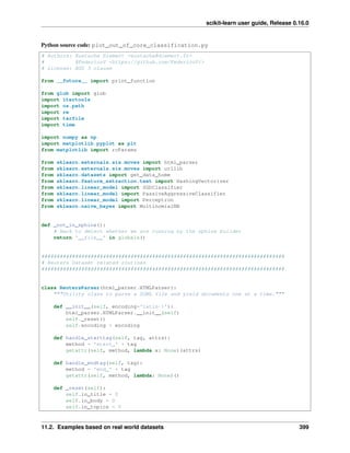
![scikit-learn user guide, Release 0.16.0
self.in_topic_d = 0
self.title = ""
self.body = ""
self.topics = []
self.topic_d = ""
def parse(self, fd):
self.docs = []
for chunk in fd:
self.feed(chunk.decode(self.encoding))
for doc in self.docs:
yield doc
self.docs = []
self.close()
def handle_data(self, data):
if self.in_body:
self.body += data
elif self.in_title:
self.title += data
elif self.in_topic_d:
self.topic_d += data
def start_reuters(self, attributes):
pass
def end_reuters(self):
self.body = re.sub(r's+', r' ', self.body)
self.docs.append({'title': self.title,
'body': self.body,
'topics': self.topics})
self._reset()
def start_title(self, attributes):
self.in_title = 1
def end_title(self):
self.in_title = 0
def start_body(self, attributes):
self.in_body = 1
def end_body(self):
self.in_body = 0
def start_topics(self, attributes):
self.in_topics = 1
def end_topics(self):
self.in_topics = 0
def start_d(self, attributes):
self.in_topic_d = 1
def end_d(self):
self.in_topic_d = 0
self.topics.append(self.topic_d)
self.topic_d = ""
400 Chapter 11. Examples](https://image.slidesharecdn.com/scikit-learn0-150409112902-conversion-gate01/85/Scikit-learn-0-16-0-user-guide-410-320.jpg)

![scikit-learn user guide, Release 0.16.0
# We learn a binary classification between the "acq" class and all the others.
# "acq" was chosen as it is more or less evenly distributed in the Reuters
# files. For other datasets, one should take care of creating a test set with
# a realistic portion of positive instances.
all_classes = np.array([0, 1])
positive_class = 'acq'
# Here are some classifiers that support the `partial_fit` method
partial_fit_classifiers = {
'SGD': SGDClassifier(),
'Perceptron': Perceptron(),
'NB Multinomial': MultinomialNB(alpha=0.01),
'Passive-Aggressive': PassiveAggressiveClassifier(),
}
def get_minibatch(doc_iter, size, pos_class=positive_class):
"""Extract a minibatch of examples, return a tuple X_text, y.
Note: size is before excluding invalid docs with no topics assigned.
"""
data = [(u'{title}nn{body}'.format(**doc), pos_class in doc['topics'])
for doc in itertools.islice(doc_iter, size)
if doc['topics']]
if not len(data):
return np.asarray([], dtype=int), np.asarray([], dtype=int)
X_text, y = zip(*data)
return X_text, np.asarray(y, dtype=int)
def iter_minibatches(doc_iter, minibatch_size):
"""Generator of minibatches."""
X_text, y = get_minibatch(doc_iter, minibatch_size)
while len(X_text):
yield X_text, y
X_text, y = get_minibatch(doc_iter, minibatch_size)
# test data statistics
test_stats = {'n_test': 0, 'n_test_pos': 0}
# First we hold out a number of examples to estimate accuracy
n_test_documents = 1000
tick = time.time()
X_test_text, y_test = get_minibatch(data_stream, 1000)
parsing_time = time.time() - tick
tick = time.time()
X_test = vectorizer.transform(X_test_text)
vectorizing_time = time.time() - tick
test_stats['n_test'] += len(y_test)
test_stats['n_test_pos'] += sum(y_test)
print("Test set is %d documents (%d positive)" % (len(y_test), sum(y_test)))
def progress(cls_name, stats):
"""Report progress information, return a string."""
duration = time.time() - stats['t0']
402 Chapter 11. Examples](https://image.slidesharecdn.com/scikit-learn0-150409112902-conversion-gate01/85/Scikit-learn-0-16-0-user-guide-412-320.jpg)
![scikit-learn user guide, Release 0.16.0
s = "%20s classifier : t" % cls_name
s += "%(n_train)6d train docs (%(n_train_pos)6d positive) " % stats
s += "%(n_test)6d test docs (%(n_test_pos)6d positive) " % test_stats
s += "accuracy: %(accuracy).3f " % stats
s += "in %.2fs (%5d docs/s)" % (duration, stats['n_train'] / duration)
return s
cls_stats = {}
for cls_name in partial_fit_classifiers:
stats = {'n_train': 0, 'n_train_pos': 0,
'accuracy': 0.0, 'accuracy_history': [(0, 0)], 't0': time.time(),
'runtime_history': [(0, 0)], 'total_fit_time': 0.0}
cls_stats[cls_name] = stats
get_minibatch(data_stream, n_test_documents)
# Discard test set
# We will feed the classifier with mini-batches of 1000 documents; this means
# we have at most 1000 docs in memory at any time. The smaller the document
# batch, the bigger the relative overhead of the partial fit methods.
minibatch_size = 1000
# Create the data_stream that parses Reuters SGML files and iterates on
# documents as a stream.
minibatch_iterators = iter_minibatches(data_stream, minibatch_size)
total_vect_time = 0.0
# Main loop : iterate on mini-batchs of examples
for i, (X_train_text, y_train) in enumerate(minibatch_iterators):
tick = time.time()
X_train = vectorizer.transform(X_train_text)
total_vect_time += time.time() - tick
for cls_name, cls in partial_fit_classifiers.items():
tick = time.time()
# update estimator with examples in the current mini-batch
cls.partial_fit(X_train, y_train, classes=all_classes)
# accumulate test accuracy stats
cls_stats[cls_name]['total_fit_time'] += time.time() - tick
cls_stats[cls_name]['n_train'] += X_train.shape[0]
cls_stats[cls_name]['n_train_pos'] += sum(y_train)
tick = time.time()
cls_stats[cls_name]['accuracy'] = cls.score(X_test, y_test)
cls_stats[cls_name]['prediction_time'] = time.time() - tick
acc_history = (cls_stats[cls_name]['accuracy'],
cls_stats[cls_name]['n_train'])
cls_stats[cls_name]['accuracy_history'].append(acc_history)
run_history = (cls_stats[cls_name]['accuracy'],
total_vect_time + cls_stats[cls_name]['total_fit_time'])
cls_stats[cls_name]['runtime_history'].append(run_history)
if i % 3 == 0:
print(progress(cls_name, cls_stats[cls_name]))
if i % 3 == 0:
11.2. Examples based on real world datasets 403](https://image.slidesharecdn.com/scikit-learn0-150409112902-conversion-gate01/85/Scikit-learn-0-16-0-user-guide-413-320.jpg)
![scikit-learn user guide, Release 0.16.0
print('n')
###############################################################################
# Plot results
###############################################################################
def plot_accuracy(x, y, x_legend):
"""Plot accuracy as a function of x."""
x = np.array(x)
y = np.array(y)
plt.title('Classification accuracy as a function of %s' % x_legend)
plt.xlabel('%s' % x_legend)
plt.ylabel('Accuracy')
plt.grid(True)
plt.plot(x, y)
rcParams['legend.fontsize'] = 10
cls_names = list(sorted(cls_stats.keys()))
# Plot accuracy evolution
plt.figure()
for _, stats in sorted(cls_stats.items()):
# Plot accuracy evolution with #examples
accuracy, n_examples = zip(*stats['accuracy_history'])
plot_accuracy(n_examples, accuracy, "training examples (#)")
ax = plt.gca()
ax.set_ylim((0.8, 1))
plt.legend(cls_names, loc='best')
plt.figure()
for _, stats in sorted(cls_stats.items()):
# Plot accuracy evolution with runtime
accuracy, runtime = zip(*stats['runtime_history'])
plot_accuracy(runtime, accuracy, 'runtime (s)')
ax = plt.gca()
ax.set_ylim((0.8, 1))
plt.legend(cls_names, loc='best')
# Plot fitting times
plt.figure()
fig = plt.gcf()
cls_runtime = []
for cls_name, stats in sorted(cls_stats.items()):
cls_runtime.append(stats['total_fit_time'])
cls_runtime.append(total_vect_time)
cls_names.append('Vectorization')
bar_colors = rcParams['axes.color_cycle'][:len(cls_names)]
ax = plt.subplot(111)
rectangles = plt.bar(range(len(cls_names)), cls_runtime, width=0.5,
color=bar_colors)
ax.set_xticks(np.linspace(0.25, len(cls_names) - 0.75, len(cls_names)))
ax.set_xticklabels(cls_names, fontsize=10)
ymax = max(cls_runtime) * 1.2
404 Chapter 11. Examples](https://image.slidesharecdn.com/scikit-learn0-150409112902-conversion-gate01/85/Scikit-learn-0-16-0-user-guide-414-320.jpg)
![scikit-learn user guide, Release 0.16.0
ax.set_ylim((0, ymax))
ax.set_ylabel('runtime (s)')
ax.set_title('Training Times')
def autolabel(rectangles):
"""attach some text vi autolabel on rectangles."""
for rect in rectangles:
height = rect.get_height()
ax.text(rect.get_x() + rect.get_width() / 2.,
1.05 * height, '%.4f' % height,
ha='center', va='bottom')
autolabel(rectangles)
plt.show()
# Plot prediction times
plt.figure()
#fig = plt.gcf()
cls_runtime = []
cls_names = list(sorted(cls_stats.keys()))
for cls_name, stats in sorted(cls_stats.items()):
cls_runtime.append(stats['prediction_time'])
cls_runtime.append(parsing_time)
cls_names.append('Read/Parsen+Feat.Extr.')
cls_runtime.append(vectorizing_time)
cls_names.append('Hashingn+Vect.')
bar_colors = rcParams['axes.color_cycle'][:len(cls_names)]
ax = plt.subplot(111)
rectangles = plt.bar(range(len(cls_names)), cls_runtime, width=0.5,
color=bar_colors)
ax.set_xticks(np.linspace(0.25, len(cls_names) - 0.75, len(cls_names)))
ax.set_xticklabels(cls_names, fontsize=8)
plt.setp(plt.xticks()[1], rotation=30)
ymax = max(cls_runtime) * 1.2
ax.set_ylim((0, ymax))
ax.set_ylabel('runtime (s)')
ax.set_title('Prediction Times (%d instances)' % n_test_documents)
autolabel(rectangles)
plt.show()
Total running time of the example: 20.08 seconds ( 0 minutes 20.08 seconds)
11.3 Biclustering
Examples concerning the sklearn.cluster.bicluster module.
11.3.1 A demo of the Spectral Co-Clustering algorithm
This example demonstrates how to generate a dataset and bicluster it using the the Spectral Co-Clustering algorithm.
The dataset is generated using the make_biclusters function, which creates a matrix of small values and im-
plants bicluster with large values. The rows and columns are then shuffled and passed to the Spectral Co-Clustering
11.3. Biclustering 405](https://image.slidesharecdn.com/scikit-learn0-150409112902-conversion-gate01/85/Scikit-learn-0-16-0-user-guide-415-320.jpg)

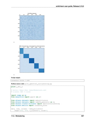
![scikit-learn user guide, Release 0.16.0
shuffle=False, random_state=0)
plt.matshow(data, cmap=plt.cm.Blues)
plt.title("Original dataset")
data, row_idx, col_idx = sg._shuffle(data, random_state=0)
plt.matshow(data, cmap=plt.cm.Blues)
plt.title("Shuffled dataset")
model = SpectralCoclustering(n_clusters=5, random_state=0)
model.fit(data)
score = consensus_score(model.biclusters_,
(rows[:, row_idx], columns[:, col_idx]))
print("consensus score: {:.3f}".format(score))
fit_data = data[np.argsort(model.row_labels_)]
fit_data = fit_data[:, np.argsort(model.column_labels_)]
plt.matshow(fit_data, cmap=plt.cm.Blues)
plt.title("After biclustering; rearranged to show biclusters")
plt.show()
Total running time of the example: 0.15 seconds ( 0 minutes 0.15 seconds)
Fig. 11.24: A demo of the Spectral Biclustering algorithm
408 Chapter 11. Examples](https://image.slidesharecdn.com/scikit-learn0-150409112902-conversion-gate01/85/Scikit-learn-0-16-0-user-guide-418-320.jpg)


![scikit-learn user guide, Release 0.16.0
shape=(300, 300), n_clusters=n_clusters, noise=10,
shuffle=False, random_state=0)
plt.matshow(data, cmap=plt.cm.Blues)
plt.title("Original dataset")
data, row_idx, col_idx = sg._shuffle(data, random_state=0)
plt.matshow(data, cmap=plt.cm.Blues)
plt.title("Shuffled dataset")
model = SpectralBiclustering(n_clusters=n_clusters, method='log',
random_state=0)
model.fit(data)
score = consensus_score(model.biclusters_,
(rows[:, row_idx], columns[:, col_idx]))
print("consensus score: {:.1f}".format(score))
fit_data = data[np.argsort(model.row_labels_)]
fit_data = fit_data[:, np.argsort(model.column_labels_)]
plt.matshow(fit_data, cmap=plt.cm.Blues)
plt.title("After biclustering; rearranged to show biclusters")
plt.matshow(np.outer(np.sort(model.row_labels_) + 1,
np.sort(model.column_labels_) + 1),
cmap=plt.cm.Blues)
plt.title("Checkerboard structure of rearranged data")
plt.show()
Total running time of the example: 0.54 seconds ( 0 minutes 0.54 seconds)
Fig. 11.25: Biclustering documents with the Spectral Co-clustering algorithm
11.3.3 Biclustering documents with the Spectral Co-clustering algorithm
This example demonstrates the Spectral Co-clustering algorithm on the twenty newsgroups dataset. The ‘comp.os.ms-
windows.misc’ category is excluded because it contains many posts containing nothing but data.
The TF-IDF vectorized posts form a word frequency matrix, which is then biclustered using Dhillon’s Spectral Co-
Clustering algorithm. The resulting document-word biclusters indicate subsets words used more often in those subsets
11.3. Biclustering 411](https://image.slidesharecdn.com/scikit-learn0-150409112902-conversion-gate01/85/Scikit-learn-0-16-0-user-guide-421-320.jpg)

![scikit-learn user guide, Release 0.16.0
def number_aware_tokenizer(doc):
""" Tokenizer that maps all numeric tokens to a placeholder.
For many applications, tokens that begin with a number are not directly
useful, but the fact that such a token exists can be relevant. By applying
this form of dimensionality reduction, some methods may perform better.
"""
token_pattern = re.compile(u'(?u)bww+b')
tokens = token_pattern.findall(doc)
tokens = ["#NUMBER" if token[0] in "0123456789_" else token
for token in tokens]
return tokens
# exclude 'comp.os.ms-windows.misc'
categories = ['alt.atheism', 'comp.graphics',
'comp.sys.ibm.pc.hardware', 'comp.sys.mac.hardware',
'comp.windows.x', 'misc.forsale', 'rec.autos',
'rec.motorcycles', 'rec.sport.baseball',
'rec.sport.hockey', 'sci.crypt', 'sci.electronics',
'sci.med', 'sci.space', 'soc.religion.christian',
'talk.politics.guns', 'talk.politics.mideast',
'talk.politics.misc', 'talk.religion.misc']
newsgroups = fetch_20newsgroups(categories=categories)
y_true = newsgroups.target
vectorizer = TfidfVectorizer(stop_words='english', min_df=5,
tokenizer=number_aware_tokenizer)
cocluster = SpectralCoclustering(n_clusters=len(categories),
svd_method='arpack', random_state=0)
kmeans = MiniBatchKMeans(n_clusters=len(categories), batch_size=20000,
random_state=0)
print("Vectorizing...")
X = vectorizer.fit_transform(newsgroups.data)
print("Coclustering...")
start_time = time()
cocluster.fit(X)
y_cocluster = cocluster.row_labels_
print("Done in {:.2f}s. V-measure: {:.4f}".format(
time() - start_time,
v_measure_score(y_cocluster, y_true)))
print("MiniBatchKMeans...")
start_time = time()
y_kmeans = kmeans.fit_predict(X)
print("Done in {:.2f}s. V-measure: {:.4f}".format(
time() - start_time,
v_measure_score(y_kmeans, y_true)))
feature_names = vectorizer.get_feature_names()
document_names = list(newsgroups.target_names[i] for i in newsgroups.target)
def bicluster_ncut(i):
rows, cols = cocluster.get_indices(i)
if not (np.any(rows) and np.any(cols)):
import sys
11.3. Biclustering 413](https://image.slidesharecdn.com/scikit-learn0-150409112902-conversion-gate01/85/Scikit-learn-0-16-0-user-guide-423-320.jpg)
![scikit-learn user guide, Release 0.16.0
return sys.float_info.max
row_complement = np.nonzero(np.logical_not(cocluster.rows_[i]))[0]
col_complement = np.nonzero(np.logical_not(cocluster.columns_[i]))[0]
weight = X[rows[:, np.newaxis], cols].sum()
cut = (X[row_complement[:, np.newaxis], cols].sum() +
X[rows[:, np.newaxis], col_complement].sum())
return cut / weight
def most_common(d):
"""Items of a defaultdict(int) with the highest values.
Like Counter.most_common in Python >=2.7.
"""
return sorted(six.iteritems(d), key=operator.itemgetter(1), reverse=True)
bicluster_ncuts = list(bicluster_ncut(i)
for i in xrange(len(newsgroups.target_names)))
best_idx = np.argsort(bicluster_ncuts)[:5]
print()
print("Best biclusters:")
print("----------------")
for idx, cluster in enumerate(best_idx):
n_rows, n_cols = cocluster.get_shape(cluster)
cluster_docs, cluster_words = cocluster.get_indices(cluster)
if not len(cluster_docs) or not len(cluster_words):
continue
# categories
counter = defaultdict(int)
for i in cluster_docs:
counter[document_names[i]] += 1
cat_string = ", ".join("{:.0f}% {}".format(float(c) / n_rows * 100, name)
for name, c in most_common(counter)[:3])
# words
out_of_cluster_docs = cocluster.row_labels_ != cluster
out_of_cluster_docs = np.where(out_of_cluster_docs)[0]
word_col = X[:, cluster_words]
word_scores = np.array(word_col[cluster_docs, :].sum(axis=0) -
word_col[out_of_cluster_docs, :].sum(axis=0))
word_scores = word_scores.ravel()
important_words = list(feature_names[cluster_words[i]]
for i in word_scores.argsort()[:-11:-1])
print("bicluster {} : {} documents, {} words".format(
idx, n_rows, n_cols))
print("categories : {}".format(cat_string))
print("words : {}n".format(', '.join(important_words)))
11.4 Calibration
Examples illustrating the calibration of predicted probabilities of classifiers.
414 Chapter 11. Examples](https://image.slidesharecdn.com/scikit-learn0-150409112902-conversion-gate01/85/Scikit-learn-0-16-0-user-guide-424-320.jpg)
![scikit-learn user guide, Release 0.16.0
Fig. 11.26: Comparison of Calibration of Classifiers
11.4.1 Comparison of Calibration of Classifiers
Well calibrated classifiers are probabilistic classifiers for which the output of the predict_proba method can be directly
interpreted as a confidence level. For instance a well calibrated (binary) classifier should classify the samples such that
among the samples to which it gave a predict_proba value close to 0.8, approx. 80% actually belong to the positive
class.
LogisticRegression returns well calibrated predictions as it directly optimizes log-loss. In contrast, the other methods
return biased probilities, with different biases per method:
• GaussianNaiveBayes tends to push probabilties to 0 or 1 (note the counts in the histograms). This is mainly
because it makes the assumption that features are conditionally independent given the class, which is not the
case in this dataset which contains 2 redundant features.
• RandomForestClassifier shows the opposite behavior: the histograms show peaks at approx. 0.2 and 0.9 prob-
ability, while probabilities close to 0 or 1 are very rare. An explanation for this is given by Niculescu-Mizil
and Caruana [1]: “Methods such as bagging and random forests that average predictions from a base set of
models can have difficulty making predictions near 0 and 1 because variance in the underlying base models will
bias predictions that should be near zero or one away from these values. Because predictions are restricted to
the interval [0,1], errors caused by variance tend to be one- sided near zero and one. For example, if a model
should predict p = 0 for a case, the only way bagging can achieve this is if all bagged trees predict zero. If we
add noise to the trees that bagging is averaging over, this noise will cause some trees to predict values larger
than 0 for this case, thus moving the average prediction of the bagged ensemble away from 0. We observe this
effect most strongly with random forests because the base-level trees trained with random forests have relatively
high variance due to feature subseting.” As a result, the calibration curve shows a characteristic sigmoid shape,
indicating that the classifier could trust its “intuition” more and return probabilties closer to 0 or 1 typically.
• Support Vector Classification (SVC) shows an even more sigmoid curve as the RandomForestClassifier, which is
typical for maximum-margin methods (compare Niculescu-Mizil and Caruana [1]), which focus on hard samples
11.4. Calibration 415](https://image.slidesharecdn.com/scikit-learn0-150409112902-conversion-gate01/85/Scikit-learn-0-16-0-user-guide-425-320.jpg)

![scikit-learn user guide, Release 0.16.0
import matplotlib.pyplot as plt
from sklearn import datasets
from sklearn.naive_bayes import GaussianNB
from sklearn.linear_model import LogisticRegression
from sklearn.ensemble import RandomForestClassifier
from sklearn.svm import LinearSVC
from sklearn.calibration import calibration_curve
X, y = datasets.make_classification(n_samples=100000, n_features=20,
n_informative=2, n_redundant=2)
train_samples = 100 # Samples used for training the models
X_train = X[:train_samples]
X_test = X[train_samples:]
y_train = y[:train_samples]
y_test = y[train_samples:]
# Create classifiers
lr = LogisticRegression()
gnb = GaussianNB()
svc = LinearSVC(C=1.0)
rfc = RandomForestClassifier(n_estimators=100)
###############################################################################
# Plot calibration plots
plt.figure(figsize=(10, 10))
ax1 = plt.subplot2grid((3, 1), (0, 0), rowspan=2)
ax2 = plt.subplot2grid((3, 1), (2, 0))
ax1.plot([0, 1], [0, 1], "k:", label="Perfectly calibrated")
for clf, name in [(lr, 'Logistic'),
(gnb, 'Naive Bayes'),
(svc, 'Support Vector Classification'),
(rfc, 'Random Forest')]:
clf.fit(X_train, y_train)
if hasattr(clf, "predict_proba"):
prob_pos = clf.predict_proba(X_test)[:, 1]
else: # use decision function
prob_pos = clf.decision_function(X_test)
prob_pos =
(prob_pos - prob_pos.min()) / (prob_pos.max() - prob_pos.min())
fraction_of_positives, mean_predicted_value =
calibration_curve(y_test, prob_pos, n_bins=10)
ax1.plot(mean_predicted_value, fraction_of_positives, "s-",
label="%s" % (name, ))
ax2.hist(prob_pos, range=(0, 1), bins=10, label=name,
histtype="step", lw=2)
ax1.set_ylabel("Fraction of positives")
ax1.set_ylim([-0.05, 1.05])
ax1.legend(loc="lower right")
ax1.set_title('Calibration plots (reliability curve)')
11.4. Calibration 417](https://image.slidesharecdn.com/scikit-learn0-150409112902-conversion-gate01/85/Scikit-learn-0-16-0-user-guide-427-320.jpg)


![scikit-learn user guide, Release 0.16.0
from sklearn.cross_validation import train_test_split
# Create dataset of classification task with many redundant and few
# informative features
X, y = datasets.make_classification(n_samples=100000, n_features=20,
n_informative=2, n_redundant=10,
random_state=42)
X_train, X_test, y_train, y_test = train_test_split(X, y, test_size=0.99,
random_state=42)
def plot_calibration_curve(est, name, fig_index):
"""Plot calibration curve for est w/o and with calibration. """
# Calibrated with isotonic calibration
isotonic = CalibratedClassifierCV(est, cv=2, method='isotonic')
# Calibrated with sigmoid calibration
sigmoid = CalibratedClassifierCV(est, cv=2, method='sigmoid')
# Logistic regression with no calibration as baseline
lr = LogisticRegression(C=1., solver='lbfgs')
fig = plt.figure(fig_index, figsize=(10, 10))
ax1 = plt.subplot2grid((3, 1), (0, 0), rowspan=2)
ax2 = plt.subplot2grid((3, 1), (2, 0))
ax1.plot([0, 1], [0, 1], "k:", label="Perfectly calibrated")
for clf, name in [(lr, 'Logistic'),
(est, name),
(isotonic, name + ' + Isotonic'),
(sigmoid, name + ' + Sigmoid')]:
clf.fit(X_train, y_train)
y_pred = clf.predict(X_test)
if hasattr(clf, "predict_proba"):
prob_pos = clf.predict_proba(X_test)[:, 1]
else: # use decision function
prob_pos = clf.decision_function(X_test)
prob_pos =
(prob_pos - prob_pos.min()) / (prob_pos.max() - prob_pos.min())
clf_score = brier_score_loss(y_test, prob_pos, pos_label=y.max())
print("%s:" % name)
print("tBrier: %1.3f" % (clf_score))
print("tPrecision: %1.3f" % precision_score(y_test, y_pred))
print("tRecall: %1.3f" % recall_score(y_test, y_pred))
print("tF1: %1.3fn" % f1_score(y_test, y_pred))
fraction_of_positives, mean_predicted_value =
calibration_curve(y_test, prob_pos, n_bins=10)
ax1.plot(mean_predicted_value, fraction_of_positives, "s-",
label="%s (%1.3f)" % (name, clf_score))
ax2.hist(prob_pos, range=(0, 1), bins=10, label=name,
histtype="step", lw=2)
11.4. Calibration 421](https://image.slidesharecdn.com/scikit-learn0-150409112902-conversion-gate01/85/Scikit-learn-0-16-0-user-guide-431-320.jpg)
![scikit-learn user guide, Release 0.16.0
ax1.set_ylabel("Fraction of positives")
ax1.set_ylim([-0.05, 1.05])
ax1.legend(loc="lower right")
ax1.set_title('Calibration plots (reliability curve)')
ax2.set_xlabel("Mean predicted value")
ax2.set_ylabel("Count")
ax2.legend(loc="upper center", ncol=2)
plt.tight_layout()
# Plot calibration cuve for Gaussian Naive Bayes
plot_calibration_curve(GaussianNB(), "Naive Bayes", 1)
# Plot calibration cuve for Linear SVC
plot_calibration_curve(LinearSVC(), "SVC", 2)
plt.show()
Total running time of the example: 1.93 seconds ( 0 minutes 1.93 seconds)
Fig. 11.28: Probability calibration of classifiers
11.4.3 Probability calibration of classifiers
When performing classification you often want to predict not only the class label, but also the associated proba-
bility. This probability gives you some kind of confidence on the prediction. However, not all classifiers pro-
vide well-calibrated probabilities, some being over-confident while others being under-confident. Thus, a sepa-
rate calibration of predicted probabilities is often desirable as a postprocessing. This example illustrates two dif-
422 Chapter 11. Examples](https://image.slidesharecdn.com/scikit-learn0-150409112902-conversion-gate01/85/Scikit-learn-0-16-0-user-guide-432-320.jpg)

![scikit-learn user guide, Release 0.16.0
from sklearn.naive_bayes import GaussianNB
from sklearn.metrics import brier_score_loss
from sklearn.calibration import CalibratedClassifierCV
from sklearn.cross_validation import train_test_split
n_samples = 50000
n_bins = 3 # use 3 bins for calibration_curve as we have 3 clusters here
# Generate 3 blobs with 2 classes where the second blob contains
# half positive samples and half negative samples. Probability in this
# blob is therefore 0.5.
centers = [(-5, -5), (0, 0), (5, 5)]
X, y = make_blobs(n_samples=n_samples, n_features=2, cluster_std=1.0,
centers=centers, shuffle=False, random_state=42)
y[:n_samples // 2] = 0
y[n_samples // 2:] = 1
sample_weight = np.random.RandomState(42).rand(y.shape[0])
# split train, test for calibration
X_train, X_test, y_train, y_test, sw_train, sw_test =
train_test_split(X, y, sample_weight, test_size=0.9, random_state=42)
# Gaussian Naive-Bayes with no calibration
clf = GaussianNB()
clf.fit(X_train, y_train) # GaussianNB itself does not support sample-weights
prob_pos_clf = clf.predict_proba(X_test)[:, 1]
# Gaussian Naive-Bayes with isotonic calibration
clf_isotonic = CalibratedClassifierCV(clf, cv=2, method='isotonic')
clf_isotonic.fit(X_train, y_train, sw_train)
prob_pos_isotonic = clf_isotonic.predict_proba(X_test)[:, 1]
# Gaussian Naive-Bayes with sigmoid calibration
clf_sigmoid = CalibratedClassifierCV(clf, cv=2, method='sigmoid')
clf_sigmoid.fit(X_train, y_train, sw_train)
prob_pos_sigmoid = clf_sigmoid.predict_proba(X_test)[:, 1]
print("Brier scores: (the smaller the better)")
clf_score = brier_score_loss(y_test, prob_pos_clf, sw_test)
print("No calibration: %1.3f" % clf_score)
clf_isotonic_score = brier_score_loss(y_test, prob_pos_isotonic, sw_test)
print("With isotonic calibration: %1.3f" % clf_isotonic_score)
clf_sigmoid_score = brier_score_loss(y_test, prob_pos_sigmoid, sw_test)
print("With sigmoid calibration: %1.3f" % clf_sigmoid_score)
###############################################################################
# Plot the data and the predicted probabilities
plt.figure()
y_unique = np.unique(y)
colors = cm.rainbow(np.linspace(0.0, 1.0, y_unique.size))
for this_y, color in zip(y_unique, colors):
this_X = X_train[y_train == this_y]
this_sw = sw_train[y_train == this_y]
424 Chapter 11. Examples](https://image.slidesharecdn.com/scikit-learn0-150409112902-conversion-gate01/85/Scikit-learn-0-16-0-user-guide-434-320.jpg)
![scikit-learn user guide, Release 0.16.0
plt.scatter(this_X[:, 0], this_X[:, 1], s=this_sw * 50, c=color, alpha=0.5,
label="Class %s" % this_y)
plt.legend(loc="best")
plt.title("Data")
plt.figure()
order = np.lexsort((prob_pos_clf, ))
plt.plot(prob_pos_clf[order], 'r', label='No calibration (%1.3f)' % clf_score)
plt.plot(prob_pos_isotonic[order], 'g', linewidth=3,
label='Isotonic calibration (%1.3f)' % clf_isotonic_score)
plt.plot(prob_pos_sigmoid[order], 'b', linewidth=3,
label='Sigmoid calibration (%1.3f)' % clf_sigmoid_score)
plt.plot(np.linspace(0, y_test.size, 51)[1::2],
y_test[order].reshape(25, -1).mean(1),
'k', linewidth=3, label=r'Empirical')
plt.ylim([-0.05, 1.05])
plt.xlabel("Instances sorted according to predicted probability "
"(uncalibrated GNB)")
plt.ylabel("P(y=1)")
plt.legend(loc="upper left")
plt.title("Gaussian naive Bayes probabilities")
plt.show()
Total running time of the example: 0.33 seconds ( 0 minutes 0.33 seconds)
Fig. 11.29: Probability Calibration for 3-class classification
11.4. Calibration 425](https://image.slidesharecdn.com/scikit-learn0-150409112902-conversion-gate01/85/Scikit-learn-0-16-0-user-guide-435-320.jpg)

![scikit-learn user guide, Release 0.16.0
import matplotlib.pyplot as plt
import numpy as np
from sklearn.datasets import make_blobs
from sklearn.ensemble import RandomForestClassifier
from sklearn.calibration import CalibratedClassifierCV
from sklearn.metrics import log_loss
np.random.seed(0)
# Generate data
X, y = make_blobs(n_samples=1000, n_features=2, random_state=42,
cluster_std=5.0)
X_train, y_train = X[:600], y[:600]
X_valid, y_valid = X[600:800], y[600:800]
X_train_valid, y_train_valid = X[:800], y[:800]
X_test, y_test = X[800:], y[800:]
# Train uncalibrated random forest classifier on whole train and validation
# data and evaluate on test data
clf = RandomForestClassifier(n_estimators=25)
clf.fit(X_train_valid, y_train_valid)
clf_probs = clf.predict_proba(X_test)
score = log_loss(y_test, clf_probs)
# Train random forest classifier, calibrate on validation data and evaluate
# on test data
clf = RandomForestClassifier(n_estimators=25)
clf.fit(X_train, y_train)
clf_probs = clf.predict_proba(X_test)
sig_clf = CalibratedClassifierCV(clf, method="sigmoid", cv="prefit")
sig_clf.fit(X_valid, y_valid)
sig_clf_probs = sig_clf.predict_proba(X_test)
sig_score = log_loss(y_test, sig_clf_probs)
# Plot changes in predicted probabilities via arrows
plt.figure(0)
colors = ["r", "g", "b"]
for i in range(clf_probs.shape[0]):
plt.arrow(clf_probs[i, 0], clf_probs[i, 1],
sig_clf_probs[i, 0] - clf_probs[i, 0],
sig_clf_probs[i, 1] - clf_probs[i, 1],
color=colors[y_test[i]], head_width=1e-2)
# Plot perfect predictions
plt.plot([1.0], [0.0], 'ro', ms=20, label="Class 1")
plt.plot([0.0], [1.0], 'go', ms=20, label="Class 2")
plt.plot([0.0], [0.0], 'bo', ms=20, label="Class 3")
# Plot boundaries of unit simplex
plt.plot([0.0, 1.0, 0.0, 0.0], [0.0, 0.0, 1.0, 0.0], 'k', label="Simplex")
# Annotate points on the simplex
plt.annotate(r'($frac{1}{3}$, $frac{1}{3}$, $frac{1}{3}$)',
xy=(1.0/3, 1.0/3), xytext=(1.0/3, .23), xycoords='data',
arrowprops=dict(facecolor='black', shrink=0.05),
horizontalalignment='center', verticalalignment='center')
11.4. Calibration 427](https://image.slidesharecdn.com/scikit-learn0-150409112902-conversion-gate01/85/Scikit-learn-0-16-0-user-guide-437-320.jpg)
![scikit-learn user guide, Release 0.16.0
plt.plot([1.0/3], [1.0/3], 'ko', ms=5)
plt.annotate(r'($frac{1}{2}$, $0$, $frac{1}{2}$)',
xy=(.5, .0), xytext=(.5, .1), xycoords='data',
arrowprops=dict(facecolor='black', shrink=0.05),
horizontalalignment='center', verticalalignment='center')
plt.annotate(r'($0$, $frac{1}{2}$, $frac{1}{2}$)',
xy=(.0, .5), xytext=(.1, .5), xycoords='data',
arrowprops=dict(facecolor='black', shrink=0.05),
horizontalalignment='center', verticalalignment='center')
plt.annotate(r'($frac{1}{2}$, $frac{1}{2}$, $0$)',
xy=(.5, .5), xytext=(.6, .6), xycoords='data',
arrowprops=dict(facecolor='black', shrink=0.05),
horizontalalignment='center', verticalalignment='center')
plt.annotate(r'($0$, $0$, $1$)',
xy=(0, 0), xytext=(.1, .1), xycoords='data',
arrowprops=dict(facecolor='black', shrink=0.05),
horizontalalignment='center', verticalalignment='center')
plt.annotate(r'($1$, $0$, $0$)',
xy=(1, 0), xytext=(1, .1), xycoords='data',
arrowprops=dict(facecolor='black', shrink=0.05),
horizontalalignment='center', verticalalignment='center')
plt.annotate(r'($0$, $1$, $0$)',
xy=(0, 1), xytext=(.1, 1), xycoords='data',
arrowprops=dict(facecolor='black', shrink=0.05),
horizontalalignment='center', verticalalignment='center')
# Add grid
plt.grid("off")
for x in [0.0, 0.1, 0.2, 0.3, 0.4, 0.5, 0.6, 0.7, 0.8, 0.9, 1.0]:
plt.plot([0, x], [x, 0], 'k', alpha=0.2)
plt.plot([0, 0 + (1-x)/2], [x, x + (1-x)/2], 'k', alpha=0.2)
plt.plot([x, x + (1-x)/2], [0, 0 + (1-x)/2], 'k', alpha=0.2)
plt.title("Change of predicted probabilities after sigmoid calibration")
plt.xlabel("Probability class 1")
plt.ylabel("Probability class 2")
plt.xlim(-0.05, 1.05)
plt.ylim(-0.05, 1.05)
plt.legend(loc="best")
print("Log-loss of")
print(" * uncalibrated classifier trained on 800 datapoints: %.3f "
% score)
print(" * classifier trained on 600 datapoints and calibrated on "
"200 datapoint: %.3f" % sig_score)
# Illustrate calibrator
plt.figure(1)
# generate grid over 2-simplex
p1d = np.linspace(0, 1, 20)
p0, p1 = np.meshgrid(p1d, p1d)
p2 = 1 - p0 - p1
p = np.c_[p0.ravel(), p1.ravel(), p2.ravel()]
p = p[p[:, 2] >= 0]
calibrated_classifier = sig_clf.calibrated_classifiers_[0]
prediction = np.vstack([calibrator.predict(this_p)
for calibrator, this_p in
zip(calibrated_classifier.calibrators_, p.T)]).T
428 Chapter 11. Examples](https://image.slidesharecdn.com/scikit-learn0-150409112902-conversion-gate01/85/Scikit-learn-0-16-0-user-guide-438-320.jpg)
![scikit-learn user guide, Release 0.16.0
prediction /= prediction.sum(axis=1)[:, None]
# Ploit modifications of calibrator
for i in range(prediction.shape[0]):
plt.arrow(p[i, 0], p[i, 1],
prediction[i, 0] - p[i, 0], prediction[i, 1] - p[i, 1],
head_width=1e-2, color=colors[np.argmax(p[i])])
# Plot boundaries of unit simplex
plt.plot([0.0, 1.0, 0.0, 0.0], [0.0, 0.0, 1.0, 0.0], 'k', label="Simplex")
plt.grid("off")
for x in [0.0, 0.1, 0.2, 0.3, 0.4, 0.5, 0.6, 0.7, 0.8, 0.9, 1.0]:
plt.plot([0, x], [x, 0], 'k', alpha=0.2)
plt.plot([0, 0 + (1-x)/2], [x, x + (1-x)/2], 'k', alpha=0.2)
plt.plot([x, x + (1-x)/2], [0, 0 + (1-x)/2], 'k', alpha=0.2)
plt.title("Illustration of sigmoid calibrator")
plt.xlabel("Probability class 1")
plt.ylabel("Probability class 2")
plt.xlim(-0.05, 1.05)
plt.ylim(-0.05, 1.05)
plt.show()
Total running time of the example: 0.52 seconds ( 0 minutes 0.52 seconds)
11.5 Classification
General examples about classification algorithms.
11.5.1 Recognizing hand-written digits
An example showing how the scikit-learn can be used to recognize images of hand-written digits.
This example is commented in the tutorial section of the user manual.
11.5. Classification 429](https://image.slidesharecdn.com/scikit-learn0-150409112902-conversion-gate01/85/Scikit-learn-0-16-0-user-guide-439-320.jpg)

![scikit-learn user guide, Release 0.16.0
Script output:
Classification report for classifier SVC(C=1.0, cache_size=200, class_weight=None, coef0=0.0, degree=
gamma=0.001, kernel='rbf', max_iter=-1, probability=False,
random_state=None, shrinking=True, tol=0.001, verbose=False):
precision recall f1-score support
0 1.00 0.99 0.99 88
1 0.99 0.97 0.98 91
2 0.99 0.99 0.99 86
3 0.98 0.87 0.92 91
4 0.99 0.96 0.97 92
5 0.95 0.97 0.96 91
6 0.99 0.99 0.99 91
7 0.96 0.99 0.97 89
8 0.94 1.00 0.97 88
9 0.93 0.98 0.95 92
avg / total 0.97 0.97 0.97 899
Confusion matrix:
[[87 0 0 0 1 0 0 0 0 0]
[ 0 88 1 0 0 0 0 0 1 1]
[ 0 0 85 1 0 0 0 0 0 0]
[ 0 0 0 79 0 3 0 4 5 0]
[ 0 0 0 0 88 0 0 0 0 4]
[ 0 0 0 0 0 88 1 0 0 2]
[ 0 1 0 0 0 0 90 0 0 0]
[ 0 0 0 0 0 1 0 88 0 0]
[ 0 0 0 0 0 0 0 0 88 0]
[ 0 0 0 1 0 1 0 0 0 90]]
Python source code: plot_digits_classification.py
print(__doc__)
# Author: Gael Varoquaux <gael dot varoquaux at normalesup dot org>
# License: BSD 3 clause
# Standard scientific Python imports
import matplotlib.pyplot as plt
# Import datasets, classifiers and performance metrics
from sklearn import datasets, svm, metrics
# The digits dataset
digits = datasets.load_digits()
# The data that we are interested in is made of 8x8 images of digits, let's
# have a look at the first 3 images, stored in the `images` attribute of the
# dataset. If we were working from image files, we could load them using
# pylab.imread. Note that each image must have the same size. For these
# images, we know which digit they represent: it is given in the 'target' of
# the dataset.
images_and_labels = list(zip(digits.images, digits.target))
for index, (image, label) in enumerate(images_and_labels[:4]):
plt.subplot(2, 4, index + 1)
plt.axis('off')
11.5. Classification 431](https://image.slidesharecdn.com/scikit-learn0-150409112902-conversion-gate01/85/Scikit-learn-0-16-0-user-guide-441-320.jpg)
![scikit-learn user guide, Release 0.16.0
plt.imshow(image, cmap=plt.cm.gray_r, interpolation='nearest')
plt.title('Training: %i' % label)
# To apply a classifier on this data, we need to flatten the image, to
# turn the data in a (samples, feature) matrix:
n_samples = len(digits.images)
data = digits.images.reshape((n_samples, -1))
# Create a classifier: a support vector classifier
classifier = svm.SVC(gamma=0.001)
# We learn the digits on the first half of the digits
classifier.fit(data[:n_samples / 2], digits.target[:n_samples / 2])
# Now predict the value of the digit on the second half:
expected = digits.target[n_samples / 2:]
predicted = classifier.predict(data[n_samples / 2:])
print("Classification report for classifier %s:n%sn"
% (classifier, metrics.classification_report(expected, predicted)))
print("Confusion matrix:n%s" % metrics.confusion_matrix(expected, predicted))
images_and_predictions = list(zip(digits.images[n_samples / 2:], predicted))
for index, (image, prediction) in enumerate(images_and_predictions[:4]):
plt.subplot(2, 4, index + 5)
plt.axis('off')
plt.imshow(image, cmap=plt.cm.gray_r, interpolation='nearest')
plt.title('Prediction: %i' % prediction)
plt.show()
Total running time of the example: 0.50 seconds ( 0 minutes 0.50 seconds)
11.5.2 Normal and Shrinkage Linear Discriminant Analysis for classification
Shows how shrinkage improves classification.
432 Chapter 11. Examples](https://image.slidesharecdn.com/scikit-learn0-150409112902-conversion-gate01/85/Scikit-learn-0-16-0-user-guide-442-320.jpg)
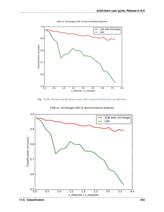
![scikit-learn user guide, Release 0.16.0
Python source code: plot_lda.py
from __future__ import division
import numpy as np
import matplotlib.pyplot as plt
from sklearn.datasets import make_blobs
from sklearn.lda import LDA
n_train = 20 # samples for training
n_test = 200 # samples for testing
n_averages = 50 # how often to repeat classification
n_features_max = 75 # maximum number of features
step = 4 # step size for the calculation
def generate_data(n_samples, n_features):
"""Generate random blob-ish data with noisy features.
This returns an array of input data with shape `(n_samples, n_features)`
and an array of `n_samples` target labels.
Only one feature contains discriminative information, the other features
contain only noise.
"""
X, y = make_blobs(n_samples=n_samples, n_features=1, centers=[[-2], [2]])
# add non-discriminative features
if n_features > 1:
X = np.hstack([X, np.random.randn(n_samples, n_features - 1)])
return X, y
acc_clf1, acc_clf2 = [], []
n_features_range = range(1, n_features_max + 1, step)
for n_features in n_features_range:
score_clf1, score_clf2 = 0, 0
for _ in range(n_averages):
X, y = generate_data(n_train, n_features)
clf1 = LDA(solver='lsqr', shrinkage='auto').fit(X, y)
clf2 = LDA(solver='lsqr', shrinkage=None).fit(X, y)
X, y = generate_data(n_test, n_features)
score_clf1 += clf1.score(X, y)
score_clf2 += clf2.score(X, y)
acc_clf1.append(score_clf1 / n_averages)
acc_clf2.append(score_clf2 / n_averages)
features_samples_ratio = np.array(n_features_range) / n_train
plt.plot(features_samples_ratio, acc_clf1, linewidth=2,
label="LDA with shrinkage", color='r')
plt.plot(features_samples_ratio, acc_clf2, linewidth=2,
label="LDA", color='g')
plt.xlabel('n_features / n_samples')
434 Chapter 11. Examples](https://image.slidesharecdn.com/scikit-learn0-150409112902-conversion-gate01/85/Scikit-learn-0-16-0-user-guide-444-320.jpg)

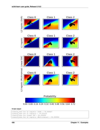
![scikit-learn user guide, Release 0.16.0
Python source code: plot_classification_probability.py
print(__doc__)
# Author: Alexandre Gramfort <alexandre.gramfort@inria.fr>
# License: BSD 3 clause
import matplotlib.pyplot as plt
import numpy as np
from sklearn.linear_model import LogisticRegression
from sklearn.svm import SVC
from sklearn import datasets
iris = datasets.load_iris()
X = iris.data[:, 0:2] # we only take the first two features for visualization
y = iris.target
n_features = X.shape[1]
C = 1.0
# Create different classifiers. The logistic regression cannot do
# multiclass out of the box.
classifiers = {'L1 logistic': LogisticRegression(C=C, penalty='l1'),
'L2 logistic (OvR)': LogisticRegression(C=C, penalty='l2'),
'Linear SVC': SVC(kernel='linear', C=C, probability=True,
random_state=0),
'L2 logistic (Multinomial)': LogisticRegression(
C=C, solver='lbfgs', multi_class='multinomial'
)}
n_classifiers = len(classifiers)
plt.figure(figsize=(3 * 2, n_classifiers * 2))
plt.subplots_adjust(bottom=.2, top=.95)
xx = np.linspace(3, 9, 100)
yy = np.linspace(1, 5, 100).T
xx, yy = np.meshgrid(xx, yy)
Xfull = np.c_[xx.ravel(), yy.ravel()]
for index, (name, classifier) in enumerate(classifiers.items()):
classifier.fit(X, y)
y_pred = classifier.predict(X)
classif_rate = np.mean(y_pred.ravel() == y.ravel()) * 100
print("classif_rate for %s : %f " % (name, classif_rate))
# View probabilities=
probas = classifier.predict_proba(Xfull)
n_classes = np.unique(y_pred).size
for k in range(n_classes):
plt.subplot(n_classifiers, n_classes, index * n_classes + k + 1)
plt.title("Class %d" % k)
if k == 0:
plt.ylabel(name)
11.5. Classification 437](https://image.slidesharecdn.com/scikit-learn0-150409112902-conversion-gate01/85/Scikit-learn-0-16-0-user-guide-447-320.jpg)
![scikit-learn user guide, Release 0.16.0
imshow_handle = plt.imshow(probas[:, k].reshape((100, 100)),
extent=(3, 9, 1, 5), origin='lower')
plt.xticks(())
plt.yticks(())
idx = (y_pred == k)
if idx.any():
plt.scatter(X[idx, 0], X[idx, 1], marker='o', c='k')
ax = plt.axes([0.15, 0.04, 0.7, 0.05])
plt.title("Probability")
plt.colorbar(imshow_handle, cax=ax, orientation='horizontal')
plt.show()
Total running time of the example: 0.71 seconds ( 0 minutes 0.71 seconds)
Fig. 11.33: Classifier comparison
11.5.4 Classifier comparison
A comparison of a several classifiers in scikit-learn on synthetic datasets. The point of this example is to illustrate
the nature of decision boundaries of different classifiers. This should be taken with a grain of salt, as the intuition
conveyed by these examples does not necessarily carry over to real datasets.
Particularly in high-dimensional spaces, data can more easily be separated linearly and the simplicity of classifiers
such as naive Bayes and linear SVMs might lead to better generalization than is achieved by other classifiers.
The plots show training points in solid colors and testing points semi-transparent. The lower right shows the classifi-
cation accuracy on the test set.
438 Chapter 11. Examples](https://image.slidesharecdn.com/scikit-learn0-150409112902-conversion-gate01/85/Scikit-learn-0-16-0-user-guide-448-320.jpg)
![scikit-learn user guide, Release 0.16.0
Python source code: plot_classifier_comparison.py
print(__doc__)
# Code source: Gaël Varoquaux
# Andreas Müller
# Modified for documentation by Jaques Grobler
# License: BSD 3 clause
import numpy as np
import matplotlib.pyplot as plt
from matplotlib.colors import ListedColormap
from sklearn.cross_validation import train_test_split
from sklearn.preprocessing import StandardScaler
from sklearn.datasets import make_moons, make_circles, make_classification
from sklearn.neighbors import KNeighborsClassifier
from sklearn.svm import SVC
from sklearn.tree import DecisionTreeClassifier
from sklearn.ensemble import RandomForestClassifier, AdaBoostClassifier
from sklearn.naive_bayes import GaussianNB
from sklearn.lda import LDA
from sklearn.qda import QDA
h = .02 # step size in the mesh
names = ["Nearest Neighbors", "Linear SVM", "RBF SVM", "Decision Tree",
"Random Forest", "AdaBoost", "Naive Bayes", "LDA", "QDA"]
classifiers = [
KNeighborsClassifier(3),
SVC(kernel="linear", C=0.025),
SVC(gamma=2, C=1),
DecisionTreeClassifier(max_depth=5),
RandomForestClassifier(max_depth=5, n_estimators=10, max_features=1),
AdaBoostClassifier(),
GaussianNB(),
LDA(),
QDA()]
X, y = make_classification(n_features=2, n_redundant=0, n_informative=2,
random_state=1, n_clusters_per_class=1)
rng = np.random.RandomState(2)
X += 2 * rng.uniform(size=X.shape)
linearly_separable = (X, y)
11.5. Classification 439](https://image.slidesharecdn.com/scikit-learn0-150409112902-conversion-gate01/85/Scikit-learn-0-16-0-user-guide-449-320.jpg)
![scikit-learn user guide, Release 0.16.0
datasets = [make_moons(noise=0.3, random_state=0),
make_circles(noise=0.2, factor=0.5, random_state=1),
linearly_separable
]
figure = plt.figure(figsize=(27, 9))
i = 1
# iterate over datasets
for ds in datasets:
# preprocess dataset, split into training and test part
X, y = ds
X = StandardScaler().fit_transform(X)
X_train, X_test, y_train, y_test = train_test_split(X, y, test_size=.4)
x_min, x_max = X[:, 0].min() - .5, X[:, 0].max() + .5
y_min, y_max = X[:, 1].min() - .5, X[:, 1].max() + .5
xx, yy = np.meshgrid(np.arange(x_min, x_max, h),
np.arange(y_min, y_max, h))
# just plot the dataset first
cm = plt.cm.RdBu
cm_bright = ListedColormap(['#FF0000', '#0000FF'])
ax = plt.subplot(len(datasets), len(classifiers) + 1, i)
# Plot the training points
ax.scatter(X_train[:, 0], X_train[:, 1], c=y_train, cmap=cm_bright)
# and testing points
ax.scatter(X_test[:, 0], X_test[:, 1], c=y_test, cmap=cm_bright, alpha=0.6)
ax.set_xlim(xx.min(), xx.max())
ax.set_ylim(yy.min(), yy.max())
ax.set_xticks(())
ax.set_yticks(())
i += 1
# iterate over classifiers
for name, clf in zip(names, classifiers):
ax = plt.subplot(len(datasets), len(classifiers) + 1, i)
clf.fit(X_train, y_train)
score = clf.score(X_test, y_test)
# Plot the decision boundary. For that, we will assign a color to each
# point in the mesh [x_min, m_max]x[y_min, y_max].
if hasattr(clf, "decision_function"):
Z = clf.decision_function(np.c_[xx.ravel(), yy.ravel()])
else:
Z = clf.predict_proba(np.c_[xx.ravel(), yy.ravel()])[:, 1]
# Put the result into a color plot
Z = Z.reshape(xx.shape)
ax.contourf(xx, yy, Z, cmap=cm, alpha=.8)
# Plot also the training points
ax.scatter(X_train[:, 0], X_train[:, 1], c=y_train, cmap=cm_bright)
# and testing points
ax.scatter(X_test[:, 0], X_test[:, 1], c=y_test, cmap=cm_bright,
alpha=0.6)
ax.set_xlim(xx.min(), xx.max())
ax.set_ylim(yy.min(), yy.max())
440 Chapter 11. Examples](https://image.slidesharecdn.com/scikit-learn0-150409112902-conversion-gate01/85/Scikit-learn-0-16-0-user-guide-450-320.jpg)

![scikit-learn user guide, Release 0.16.0
Python source code: plot_lda_qda.py
print(__doc__)
from scipy import linalg
import numpy as np
import matplotlib.pyplot as plt
import matplotlib as mpl
from matplotlib import colors
from sklearn.lda import LDA
from sklearn.qda import QDA
###############################################################################
# colormap
cmap = colors.LinearSegmentedColormap(
'red_blue_classes',
{'red': [(0, 1, 1), (1, 0.7, 0.7)],
'green': [(0, 0.7, 0.7), (1, 0.7, 0.7)],
'blue': [(0, 0.7, 0.7), (1, 1, 1)]})
plt.cm.register_cmap(cmap=cmap)
###############################################################################
# generate datasets
def dataset_fixed_cov():
442 Chapter 11. Examples](https://image.slidesharecdn.com/scikit-learn0-150409112902-conversion-gate01/85/Scikit-learn-0-16-0-user-guide-452-320.jpg)
![scikit-learn user guide, Release 0.16.0
'''Generate 2 Gaussians samples with the same covariance matrix'''
n, dim = 300, 2
np.random.seed(0)
C = np.array([[0., -0.23], [0.83, .23]])
X = np.r_[np.dot(np.random.randn(n, dim), C),
np.dot(np.random.randn(n, dim), C) + np.array([1, 1])]
y = np.hstack((np.zeros(n), np.ones(n)))
return X, y
def dataset_cov():
'''Generate 2 Gaussians samples with different covariance matrices'''
n, dim = 300, 2
np.random.seed(0)
C = np.array([[0., -1.], [2.5, .7]]) * 2.
X = np.r_[np.dot(np.random.randn(n, dim), C),
np.dot(np.random.randn(n, dim), C.T) + np.array([1, 4])]
y = np.hstack((np.zeros(n), np.ones(n)))
return X, y
###############################################################################
# plot functions
def plot_data(lda, X, y, y_pred, fig_index):
splot = plt.subplot(2, 2, fig_index)
if fig_index == 1:
plt.title('Linear Discriminant Analysis')
plt.ylabel('Data with fixed covariance')
elif fig_index == 2:
plt.title('Quadratic Discriminant Analysis')
elif fig_index == 3:
plt.ylabel('Data with varying covariances')
tp = (y == y_pred) # True Positive
tp0, tp1 = tp[y == 0], tp[y == 1]
X0, X1 = X[y == 0], X[y == 1]
X0_tp, X0_fp = X0[tp0], X0[~tp0]
X1_tp, X1_fp = X1[tp1], X1[~tp1]
xmin, xmax = X[:, 0].min(), X[:, 0].max()
ymin, ymax = X[:, 1].min(), X[:, 1].max()
# class 0: dots
plt.plot(X0_tp[:, 0], X0_tp[:, 1], 'o', color='red')
plt.plot(X0_fp[:, 0], X0_fp[:, 1], '.', color='#990000') # dark red
# class 1: dots
plt.plot(X1_tp[:, 0], X1_tp[:, 1], 'o', color='blue')
plt.plot(X1_fp[:, 0], X1_fp[:, 1], '.', color='#000099') # dark blue
# class 0 and 1 : areas
nx, ny = 200, 100
x_min, x_max = plt.xlim()
y_min, y_max = plt.ylim()
xx, yy = np.meshgrid(np.linspace(x_min, x_max, nx),
np.linspace(y_min, y_max, ny))
Z = lda.predict_proba(np.c_[xx.ravel(), yy.ravel()])
Z = Z[:, 1].reshape(xx.shape)
plt.pcolormesh(xx, yy, Z, cmap='red_blue_classes',
11.5. Classification 443](https://image.slidesharecdn.com/scikit-learn0-150409112902-conversion-gate01/85/Scikit-learn-0-16-0-user-guide-453-320.jpg)
![scikit-learn user guide, Release 0.16.0
norm=colors.Normalize(0., 1.))
plt.contour(xx, yy, Z, [0.5], linewidths=2., colors='k')
# means
plt.plot(lda.means_[0][0], lda.means_[0][1],
'o', color='black', markersize=10)
plt.plot(lda.means_[1][0], lda.means_[1][1],
'o', color='black', markersize=10)
return splot
def plot_ellipse(splot, mean, cov, color):
v, w = linalg.eigh(cov)
u = w[0] / linalg.norm(w[0])
angle = np.arctan(u[1] / u[0])
angle = 180 * angle / np.pi # convert to degrees
# filled Gaussian at 2 standard deviation
ell = mpl.patches.Ellipse(mean, 2 * v[0] ** 0.5, 2 * v[1] ** 0.5,
180 + angle, color=color)
ell.set_clip_box(splot.bbox)
ell.set_alpha(0.5)
splot.add_artist(ell)
splot.set_xticks(())
splot.set_yticks(())
def plot_lda_cov(lda, splot):
plot_ellipse(splot, lda.means_[0], lda.covariance_, 'red')
plot_ellipse(splot, lda.means_[1], lda.covariance_, 'blue')
def plot_qda_cov(qda, splot):
plot_ellipse(splot, qda.means_[0], qda.covariances_[0], 'red')
plot_ellipse(splot, qda.means_[1], qda.covariances_[1], 'blue')
###############################################################################
for i, (X, y) in enumerate([dataset_fixed_cov(), dataset_cov()]):
# LDA
lda = LDA(solver="svd", store_covariance=True)
y_pred = lda.fit(X, y).predict(X)
splot = plot_data(lda, X, y, y_pred, fig_index=2 * i + 1)
plot_lda_cov(lda, splot)
plt.axis('tight')
# QDA
qda = QDA()
y_pred = qda.fit(X, y, store_covariances=True).predict(X)
splot = plot_data(qda, X, y, y_pred, fig_index=2 * i + 2)
plot_qda_cov(qda, splot)
plt.axis('tight')
plt.suptitle('LDA vs QDA')
plt.show()
Total running time of the example: 0.32 seconds ( 0 minutes 0.32 seconds)
444 Chapter 11. Examples](https://image.slidesharecdn.com/scikit-learn0-150409112902-conversion-gate01/85/Scikit-learn-0-16-0-user-guide-454-320.jpg)

![scikit-learn user guide, Release 0.16.0
Script output:
number of estimated clusters : 3
Python source code: plot_mean_shift.py
print(__doc__)
import numpy as np
from sklearn.cluster import MeanShift, estimate_bandwidth
from sklearn.datasets.samples_generator import make_blobs
###############################################################################
# Generate sample data
centers = [[1, 1], [-1, -1], [1, -1]]
X, _ = make_blobs(n_samples=10000, centers=centers, cluster_std=0.6)
###############################################################################
# Compute clustering with MeanShift
# The following bandwidth can be automatically detected using
bandwidth = estimate_bandwidth(X, quantile=0.2, n_samples=500)
ms = MeanShift(bandwidth=bandwidth, bin_seeding=True)
ms.fit(X)
labels = ms.labels_
cluster_centers = ms.cluster_centers_
446 Chapter 11. Examples](https://image.slidesharecdn.com/scikit-learn0-150409112902-conversion-gate01/85/Scikit-learn-0-16-0-user-guide-456-320.jpg)
![scikit-learn user guide, Release 0.16.0
labels_unique = np.unique(labels)
n_clusters_ = len(labels_unique)
print("number of estimated clusters : %d" % n_clusters_)
###############################################################################
# Plot result
import matplotlib.pyplot as plt
from itertools import cycle
plt.figure(1)
plt.clf()
colors = cycle('bgrcmykbgrcmykbgrcmykbgrcmyk')
for k, col in zip(range(n_clusters_), colors):
my_members = labels == k
cluster_center = cluster_centers[k]
plt.plot(X[my_members, 0], X[my_members, 1], col + '.')
plt.plot(cluster_center[0], cluster_center[1], 'o', markerfacecolor=col,
markeredgecolor='k', markersize=14)
plt.title('Estimated number of clusters: %d' % n_clusters_)
plt.show()
Total running time of the example: 0.32 seconds ( 0 minutes 0.32 seconds)
Fig. 11.36: A demo of structured Ward hierarchical clustering on Lena image
11.6. Clustering 447](https://image.slidesharecdn.com/scikit-learn0-150409112902-conversion-gate01/85/Scikit-learn-0-16-0-user-guide-457-320.jpg)
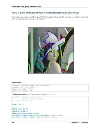
![scikit-learn user guide, Release 0.16.0
###############################################################################
# Generate data
lena = sp.misc.lena()
# Downsample the image by a factor of 4
lena = lena[::2, ::2] + lena[1::2, ::2] + lena[::2, 1::2] + lena[1::2, 1::2]
X = np.reshape(lena, (-1, 1))
###############################################################################
# Define the structure A of the data. Pixels connected to their neighbors.
connectivity = grid_to_graph(*lena.shape)
###############################################################################
# Compute clustering
print("Compute structured hierarchical clustering...")
st = time.time()
n_clusters = 15 # number of regions
ward = AgglomerativeClustering(n_clusters=n_clusters,
linkage='ward', connectivity=connectivity).fit(X)
label = np.reshape(ward.labels_, lena.shape)
print("Elapsed time: ", time.time() - st)
print("Number of pixels: ", label.size)
print("Number of clusters: ", np.unique(label).size)
###############################################################################
# Plot the results on an image
plt.figure(figsize=(5, 5))
plt.imshow(lena, cmap=plt.cm.gray)
for l in range(n_clusters):
plt.contour(label == l, contours=1,
colors=[plt.cm.spectral(l / float(n_clusters)), ])
plt.xticks(())
plt.yticks(())
plt.show()
Total running time of the example: 7.75 seconds ( 0 minutes 7.75 seconds)
11.6.3 Feature agglomeration
These images how similar features are merged together using feature agglomeration.
11.6. Clustering 449](https://image.slidesharecdn.com/scikit-learn0-150409112902-conversion-gate01/85/Scikit-learn-0-16-0-user-guide-459-320.jpg)

![scikit-learn user guide, Release 0.16.0
# License: BSD 3 clause
import numpy as np
import matplotlib.pyplot as plt
from sklearn import datasets, cluster
from sklearn.feature_extraction.image import grid_to_graph
digits = datasets.load_digits()
images = digits.images
X = np.reshape(images, (len(images), -1))
connectivity = grid_to_graph(*images[0].shape)
agglo = cluster.FeatureAgglomeration(connectivity=connectivity,
n_clusters=32)
agglo.fit(X)
X_reduced = agglo.transform(X)
X_restored = agglo.inverse_transform(X_reduced)
images_restored = np.reshape(X_restored, images.shape)
plt.figure(1, figsize=(4, 3.5))
plt.clf()
plt.subplots_adjust(left=.01, right=.99, bottom=.01, top=.91)
for i in range(4):
plt.subplot(3, 4, i + 1)
plt.imshow(images[i], cmap=plt.cm.gray, vmax=16, interpolation='nearest')
plt.xticks(())
plt.yticks(())
if i == 1:
plt.title('Original data')
plt.subplot(3, 4, 4 + i + 1)
plt.imshow(images_restored[i], cmap=plt.cm.gray, vmax=16,
interpolation='nearest')
if i == 1:
plt.title('Agglomerated data')
plt.xticks(())
plt.yticks(())
plt.subplot(3, 4, 10)
plt.imshow(np.reshape(agglo.labels_, images[0].shape),
interpolation='nearest', cmap=plt.cm.spectral)
plt.xticks(())
plt.yticks(())
plt.title('Labels')
plt.show()
Total running time of the example: 0.55 seconds ( 0 minutes 0.55 seconds)
11.6.4 Demo of affinity propagation clustering algorithm
Reference: Brendan J. Frey and Delbert Dueck, “Clustering by Passing Messages Between Data Points”, Science Feb.
2007
11.6. Clustering 451](https://image.slidesharecdn.com/scikit-learn0-150409112902-conversion-gate01/85/Scikit-learn-0-16-0-user-guide-461-320.jpg)

![scikit-learn user guide, Release 0.16.0
Script output:
Estimated number of clusters: 3
Homogeneity: 0.872
Completeness: 0.872
V-measure: 0.872
Adjusted Rand Index: 0.912
Adjusted Mutual Information: 0.871
Silhouette Coefficient: 0.753
Python source code: plot_affinity_propagation.py
print(__doc__)
from sklearn.cluster import AffinityPropagation
from sklearn import metrics
from sklearn.datasets.samples_generator import make_blobs
##############################################################################
# Generate sample data
centers = [[1, 1], [-1, -1], [1, -1]]
X, labels_true = make_blobs(n_samples=300, centers=centers, cluster_std=0.5,
random_state=0)
##############################################################################
# Compute Affinity Propagation
af = AffinityPropagation(preference=-50).fit(X)
cluster_centers_indices = af.cluster_centers_indices_
labels = af.labels_
n_clusters_ = len(cluster_centers_indices)
print('Estimated number of clusters: %d' % n_clusters_)
print("Homogeneity: %0.3f" % metrics.homogeneity_score(labels_true, labels))
print("Completeness: %0.3f" % metrics.completeness_score(labels_true, labels))
print("V-measure: %0.3f" % metrics.v_measure_score(labels_true, labels))
print("Adjusted Rand Index: %0.3f"
% metrics.adjusted_rand_score(labels_true, labels))
print("Adjusted Mutual Information: %0.3f"
% metrics.adjusted_mutual_info_score(labels_true, labels))
print("Silhouette Coefficient: %0.3f"
% metrics.silhouette_score(X, labels, metric='sqeuclidean'))
##############################################################################
# Plot result
import matplotlib.pyplot as plt
from itertools import cycle
plt.close('all')
plt.figure(1)
plt.clf()
colors = cycle('bgrcmykbgrcmykbgrcmykbgrcmyk')
for k, col in zip(range(n_clusters_), colors):
class_members = labels == k
cluster_center = X[cluster_centers_indices[k]]
plt.plot(X[class_members, 0], X[class_members, 1], col + '.')
plt.plot(cluster_center[0], cluster_center[1], 'o', markerfacecolor=col,
markeredgecolor='k', markersize=14)
11.6. Clustering 453](https://image.slidesharecdn.com/scikit-learn0-150409112902-conversion-gate01/85/Scikit-learn-0-16-0-user-guide-463-320.jpg)
![scikit-learn user guide, Release 0.16.0
for x in X[class_members]:
plt.plot([cluster_center[0], x[0]], [cluster_center[1], x[1]], col)
plt.title('Estimated number of clusters: %d' % n_clusters_)
plt.show()
Total running time of the example: 0.77 seconds ( 0 minutes 0.77 seconds)
Fig. 11.39: Agglomerative clustering with and without structure
11.6.5 Agglomerative clustering with and without structure
This example shows the effect of imposing a connectivity graph to capture local structure in the data. The graph is
simply the graph of 20 nearest neighbors.
Two consequences of imposing a connectivity can be seen. First clustering with a connectivity matrix is much faster.
Second, when using a connectivity matrix, average and complete linkage are unstable and tend to create a few clusters
that grow very quickly. Indeed, average and complete linkage fight this percolation behavior by considering all the
distances between two clusters when merging them. The connectivity graph breaks this mechanism. This effect is more
pronounced for very sparse graphs (try decreasing the number of neighbors in kneighbors_graph) and with complete
linkage. In particular, having a very small number of neighbors in the graph, imposes a geometry that is close to that
of single linkage, which is well known to have this percolation instability.
454 Chapter 11. Examples](https://image.slidesharecdn.com/scikit-learn0-150409112902-conversion-gate01/85/Scikit-learn-0-16-0-user-guide-464-320.jpg)

![scikit-learn user guide, Release 0.16.0
# time. A very large number of neighbors gives more evenly distributed
# cluster sizes, but may not impose the local manifold structure of
# the data
knn_graph = kneighbors_graph(X, 30, include_self=False)
for connectivity in (None, knn_graph):
for n_clusters in (30, 3):
plt.figure(figsize=(10, 4))
for index, linkage in enumerate(('average', 'complete', 'ward')):
plt.subplot(1, 3, index + 1)
model = AgglomerativeClustering(linkage=linkage,
connectivity=connectivity,
n_clusters=n_clusters)
t0 = time.time()
model.fit(X)
elapsed_time = time.time() - t0
plt.scatter(X[:, 0], X[:, 1], c=model.labels_,
cmap=plt.cm.spectral)
plt.title('linkage=%s (time %.2fs)' % (linkage, elapsed_time),
fontdict=dict(verticalalignment='top'))
plt.axis('equal')
plt.axis('off')
plt.subplots_adjust(bottom=0, top=.89, wspace=0,
left=0, right=1)
plt.suptitle('n_cluster=%i, connectivity=%r' %
(n_clusters, connectivity is not None), size=17)
plt.show()
Total running time of the example: 8.85 seconds ( 0 minutes 8.85 seconds)
11.6.6 Segmenting the picture of Lena in regions
This example uses Spectral clustering on a graph created from voxel-to-voxel difference on an image to break this
image into multiple partly-homogeneous regions.
This procedure (spectral clustering on an image) is an efficient approximate solution for finding normalized graph cuts.
There are two options to assign labels:
• with ‘kmeans’ spectral clustering will cluster samples in the embedding space using a kmeans algorithm
• whereas ‘discrete’ will iteratively search for the closest partition space to the embedding space.
456 Chapter 11. Examples](https://image.slidesharecdn.com/scikit-learn0-150409112902-conversion-gate01/85/Scikit-learn-0-16-0-user-guide-466-320.jpg)
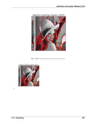
![scikit-learn user guide, Release 0.16.0
•
Python source code: plot_lena_segmentation.py
print(__doc__)
# Author: Gael Varoquaux <gael.varoquaux@normalesup.org>, Brian Cheung
# License: BSD 3 clause
import time
import numpy as np
import scipy as sp
import matplotlib.pyplot as plt
from sklearn.feature_extraction import image
from sklearn.cluster import spectral_clustering
lena = sp.misc.lena()
# Downsample the image by a factor of 4
lena = lena[::2, ::2] + lena[1::2, ::2] + lena[::2, 1::2] + lena[1::2, 1::2]
lena = lena[::2, ::2] + lena[1::2, ::2] + lena[::2, 1::2] + lena[1::2, 1::2]
# Convert the image into a graph with the value of the gradient on the
# edges.
graph = image.img_to_graph(lena)
# Take a decreasing function of the gradient: an exponential
# The smaller beta is, the more independent the segmentation is of the
# actual image. For beta=1, the segmentation is close to a voronoi
beta = 5
eps = 1e-6
graph.data = np.exp(-beta * graph.data / lena.std()) + eps
# Apply spectral clustering (this step goes much faster if you have pyamg
# installed)
N_REGIONS = 11
###############################################################################
# Visualize the resulting regions
for assign_labels in ('kmeans', 'discretize'):
t0 = time.time()
labels = spectral_clustering(graph, n_clusters=N_REGIONS,
assign_labels=assign_labels,
458 Chapter 11. Examples](https://image.slidesharecdn.com/scikit-learn0-150409112902-conversion-gate01/85/Scikit-learn-0-16-0-user-guide-468-320.jpg)
![scikit-learn user guide, Release 0.16.0
random_state=1)
t1 = time.time()
labels = labels.reshape(lena.shape)
plt.figure(figsize=(5, 5))
plt.imshow(lena, cmap=plt.cm.gray)
for l in range(N_REGIONS):
plt.contour(labels == l, contours=1,
colors=[plt.cm.spectral(l / float(N_REGIONS)), ])
plt.xticks(())
plt.yticks(())
plt.title('Spectral clustering: %s, %.2fs' % (assign_labels, (t1 - t0)))
plt.show()
Total running time of the example: 61.87 seconds ( 1 minutes 1.87 seconds)
Fig. 11.41: Demo of DBSCAN clustering algorithm
11.6.7 Demo of DBSCAN clustering algorithm
Finds core samples of high density and expands clusters from them.
11.6. Clustering 459](https://image.slidesharecdn.com/scikit-learn0-150409112902-conversion-gate01/85/Scikit-learn-0-16-0-user-guide-469-320.jpg)
![scikit-learn user guide, Release 0.16.0
Script output:
Estimated number of clusters: 3
Homogeneity: 0.953
Completeness: 0.883
V-measure: 0.917
Adjusted Rand Index: 0.952
Adjusted Mutual Information: 0.883
Silhouette Coefficient: 0.626
Python source code: plot_dbscan.py
print(__doc__)
import numpy as np
from sklearn.cluster import DBSCAN
from sklearn import metrics
from sklearn.datasets.samples_generator import make_blobs
from sklearn.preprocessing import StandardScaler
##############################################################################
# Generate sample data
centers = [[1, 1], [-1, -1], [1, -1]]
X, labels_true = make_blobs(n_samples=750, centers=centers, cluster_std=0.4,
random_state=0)
460 Chapter 11. Examples](https://image.slidesharecdn.com/scikit-learn0-150409112902-conversion-gate01/85/Scikit-learn-0-16-0-user-guide-470-320.jpg)
![scikit-learn user guide, Release 0.16.0
X = StandardScaler().fit_transform(X)
##############################################################################
# Compute DBSCAN
db = DBSCAN(eps=0.3, min_samples=10).fit(X)
core_samples_mask = np.zeros_like(db.labels_, dtype=bool)
core_samples_mask[db.core_sample_indices_] = True
labels = db.labels_
# Number of clusters in labels, ignoring noise if present.
n_clusters_ = len(set(labels)) - (1 if -1 in labels else 0)
print('Estimated number of clusters: %d' % n_clusters_)
print("Homogeneity: %0.3f" % metrics.homogeneity_score(labels_true, labels))
print("Completeness: %0.3f" % metrics.completeness_score(labels_true, labels))
print("V-measure: %0.3f" % metrics.v_measure_score(labels_true, labels))
print("Adjusted Rand Index: %0.3f"
% metrics.adjusted_rand_score(labels_true, labels))
print("Adjusted Mutual Information: %0.3f"
% metrics.adjusted_mutual_info_score(labels_true, labels))
print("Silhouette Coefficient: %0.3f"
% metrics.silhouette_score(X, labels))
##############################################################################
# Plot result
import matplotlib.pyplot as plt
# Black removed and is used for noise instead.
unique_labels = set(labels)
colors = plt.cm.Spectral(np.linspace(0, 1, len(unique_labels)))
for k, col in zip(unique_labels, colors):
if k == -1:
# Black used for noise.
col = 'k'
class_member_mask = (labels == k)
xy = X[class_member_mask & core_samples_mask]
plt.plot(xy[:, 0], xy[:, 1], 'o', markerfacecolor=col,
markeredgecolor='k', markersize=14)
xy = X[class_member_mask & ~core_samples_mask]
plt.plot(xy[:, 0], xy[:, 1], 'o', markerfacecolor=col,
markeredgecolor='k', markersize=6)
plt.title('Estimated number of clusters: %d' % n_clusters_)
plt.show()
Total running time of the example: 0.24 seconds ( 0 minutes 0.24 seconds)
11.6.8 Online learning of a dictionary of parts of faces
This example uses a large dataset of faces to learn a set of 20 x 20 images patches that constitute faces.
From the programming standpoint, it is interesting because it shows how to use the online API of the scikit-learn to
process a very large dataset by chunks. The way we proceed is that we load an image at a time and extract randomly
11.6. Clustering 461](https://image.slidesharecdn.com/scikit-learn0-150409112902-conversion-gate01/85/Scikit-learn-0-16-0-user-guide-471-320.jpg)
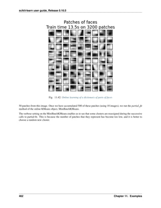
![scikit-learn user guide, Release 0.16.0
Script output:
Learning the dictionary...
Partial fit of 100 out of 2400
Partial fit of 200 out of 2400
[MiniBatchKMeans] Reassigning 16 cluster centers.
Partial fit of 300 out of 2400
Partial fit of 400 out of 2400
Partial fit of 500 out of 2400
Partial fit of 600 out of 2400
Partial fit of 700 out of 2400
Partial fit of 800 out of 2400
Partial fit of 900 out of 2400
Partial fit of 1000 out of 2400
Partial fit of 1100 out of 2400
Partial fit of 1200 out of 2400
Partial fit of 1300 out of 2400
Partial fit of 1400 out of 2400
Partial fit of 1500 out of 2400
Partial fit of 1600 out of 2400
Partial fit of 1700 out of 2400
Partial fit of 1800 out of 2400
Partial fit of 1900 out of 2400
Partial fit of 2000 out of 2400
Partial fit of 2100 out of 2400
Partial fit of 2200 out of 2400
Partial fit of 2300 out of 2400
Partial fit of 2400 out of 2400
done in 13.50s.
Python source code: plot_dict_face_patches.py
11.6. Clustering 463](https://image.slidesharecdn.com/scikit-learn0-150409112902-conversion-gate01/85/Scikit-learn-0-16-0-user-guide-473-320.jpg)
![scikit-learn user guide, Release 0.16.0
print(__doc__)
import time
import matplotlib.pyplot as plt
import numpy as np
from sklearn import datasets
from sklearn.cluster import MiniBatchKMeans
from sklearn.feature_extraction.image import extract_patches_2d
faces = datasets.fetch_olivetti_faces()
###############################################################################
# Learn the dictionary of images
print('Learning the dictionary... ')
rng = np.random.RandomState(0)
kmeans = MiniBatchKMeans(n_clusters=81, random_state=rng, verbose=True)
patch_size = (20, 20)
buffer = []
index = 1
t0 = time.time()
# The online learning part: cycle over the whole dataset 6 times
index = 0
for _ in range(6):
for img in faces.images:
data = extract_patches_2d(img, patch_size, max_patches=50,
random_state=rng)
data = np.reshape(data, (len(data), -1))
buffer.append(data)
index += 1
if index % 10 == 0:
data = np.concatenate(buffer, axis=0)
data -= np.mean(data, axis=0)
data /= np.std(data, axis=0)
kmeans.partial_fit(data)
buffer = []
if index % 100 == 0:
print('Partial fit of %4i out of %i'
% (index, 6 * len(faces.images)))
dt = time.time() - t0
print('done in %.2fs.' % dt)
###############################################################################
# Plot the results
plt.figure(figsize=(4.2, 4))
for i, patch in enumerate(kmeans.cluster_centers_):
plt.subplot(9, 9, i + 1)
plt.imshow(patch.reshape(patch_size), cmap=plt.cm.gray,
interpolation='nearest')
plt.xticks(())
plt.yticks(())
464 Chapter 11. Examples](https://image.slidesharecdn.com/scikit-learn0-150409112902-conversion-gate01/85/Scikit-learn-0-16-0-user-guide-474-320.jpg)


![scikit-learn user guide, Release 0.16.0
# equal bins lena
regular_values = np.linspace(0, 256, n_clusters + 1)
regular_labels = np.searchsorted(regular_values, lena) - 1
regular_values = .5 * (regular_values[1:] + regular_values[:-1]) # mean
regular_lena = np.choose(regular_labels.ravel(), regular_values)
regular_lena.shape = lena.shape
plt.figure(3, figsize=(3, 2.2))
plt.imshow(regular_lena, cmap=plt.cm.gray, vmin=vmin, vmax=vmax)
# histogram
plt.figure(4, figsize=(3, 2.2))
plt.clf()
plt.axes([.01, .01, .98, .98])
plt.hist(X, bins=256, color='.5', edgecolor='.5')
plt.yticks(())
plt.xticks(regular_values)
values = np.sort(values)
for center_1, center_2 in zip(values[:-1], values[1:]):
plt.axvline(.5 * (center_1 + center_2), color='b')
for center_1, center_2 in zip(regular_values[:-1], regular_values[1:]):
plt.axvline(.5 * (center_1 + center_2), color='b', linestyle='--')
plt.show()
Total running time of the example: 1.62 seconds ( 0 minutes 1.62 seconds)
Fig. 11.44: Hierarchical clustering: structured vs unstructured ward
11.6. Clustering 467](https://image.slidesharecdn.com/scikit-learn0-150409112902-conversion-gate01/85/Scikit-learn-0-16-0-user-guide-477-320.jpg)
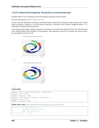
![scikit-learn user guide, Release 0.16.0
print(__doc__)
import time as time
import numpy as np
import matplotlib.pyplot as plt
import mpl_toolkits.mplot3d.axes3d as p3
from sklearn.cluster import AgglomerativeClustering
from sklearn.datasets.samples_generator import make_swiss_roll
###############################################################################
# Generate data (swiss roll dataset)
n_samples = 1500
noise = 0.05
X, _ = make_swiss_roll(n_samples, noise)
# Make it thinner
X[:, 1] *= .5
###############################################################################
# Compute clustering
print("Compute unstructured hierarchical clustering...")
st = time.time()
ward = AgglomerativeClustering(n_clusters=6, linkage='ward').fit(X)
elapsed_time = time.time() - st
label = ward.labels_
print("Elapsed time: %.2fs" % elapsed_time)
print("Number of points: %i" % label.size)
###############################################################################
# Plot result
fig = plt.figure()
ax = p3.Axes3D(fig)
ax.view_init(7, -80)
for l in np.unique(label):
ax.plot3D(X[label == l, 0], X[label == l, 1], X[label == l, 2],
'o', color=plt.cm.jet(np.float(l) / np.max(label + 1)))
plt.title('Without connectivity constraints (time %.2fs)' % elapsed_time)
###############################################################################
# Define the structure A of the data. Here a 10 nearest neighbors
from sklearn.neighbors import kneighbors_graph
connectivity = kneighbors_graph(X, n_neighbors=10, include_self=False)
###############################################################################
# Compute clustering
print("Compute structured hierarchical clustering...")
st = time.time()
ward = AgglomerativeClustering(n_clusters=6, connectivity=connectivity,
linkage='ward').fit(X)
elapsed_time = time.time() - st
label = ward.labels_
print("Elapsed time: %.2fs" % elapsed_time)
print("Number of points: %i" % label.size)
###############################################################################
# Plot result
fig = plt.figure()
ax = p3.Axes3D(fig)
11.6. Clustering 469](https://image.slidesharecdn.com/scikit-learn0-150409112902-conversion-gate01/85/Scikit-learn-0-16-0-user-guide-479-320.jpg)
![scikit-learn user guide, Release 0.16.0
ax.view_init(7, -80)
for l in np.unique(label):
ax.plot3D(X[label == l, 0], X[label == l, 1], X[label == l, 2],
'o', color=plt.cm.jet(float(l) / np.max(label + 1)))
plt.title('With connectivity constraints (time %.2fs)' % elapsed_time)
plt.show()
Total running time of the example: 0.90 seconds ( 0 minutes 0.90 seconds)
Fig. 11.45: Spectral clustering for image segmentation
11.6.11 Spectral clustering for image segmentation
In this example, an image with connected circles is generated and spectral clustering is used to separate the circles.
In these settings, the Spectral clustering approach solves the problem know as ‘normalized graph cuts’: the image is
seen as a graph of connected voxels, and the spectral clustering algorithm amounts to choosing graph cuts defining
regions while minimizing the ratio of the gradient along the cut, and the volume of the region.
As the algorithm tries to balance the volume (ie balance the region sizes), if we take circles with different sizes, the
segmentation fails.
In addition, as there is no useful information in the intensity of the image, or its gradient, we choose to perform the
spectral clustering on a graph that is only weakly informed by the gradient. This is close to performing a Voronoi
partition of the graph.
In addition, we use the mask of the objects to restrict the graph to the outline of the objects. In this example, we are
interested in separating the objects one from the other, and not from the background.
470 Chapter 11. Examples](https://image.slidesharecdn.com/scikit-learn0-150409112902-conversion-gate01/85/Scikit-learn-0-16-0-user-guide-480-320.jpg)
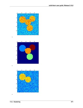
![scikit-learn user guide, Release 0.16.0
•
Python source code: plot_segmentation_toy.py
print(__doc__)
# Authors: Emmanuelle Gouillart <emmanuelle.gouillart@normalesup.org>
# Gael Varoquaux <gael.varoquaux@normalesup.org>
# License: BSD 3 clause
import numpy as np
import matplotlib.pyplot as plt
from sklearn.feature_extraction import image
from sklearn.cluster import spectral_clustering
###############################################################################
l = 100
x, y = np.indices((l, l))
center1 = (28, 24)
center2 = (40, 50)
center3 = (67, 58)
center4 = (24, 70)
radius1, radius2, radius3, radius4 = 16, 14, 15, 14
circle1 = (x - center1[0]) ** 2 + (y - center1[1]) ** 2 < radius1 ** 2
circle2 = (x - center2[0]) ** 2 + (y - center2[1]) ** 2 < radius2 ** 2
circle3 = (x - center3[0]) ** 2 + (y - center3[1]) ** 2 < radius3 ** 2
circle4 = (x - center4[0]) ** 2 + (y - center4[1]) ** 2 < radius4 ** 2
###############################################################################
# 4 circles
img = circle1 + circle2 + circle3 + circle4
mask = img.astype(bool)
img = img.astype(float)
img += 1 + 0.2 * np.random.randn(*img.shape)
# Convert the image into a graph with the value of the gradient on the
# edges.
472 Chapter 11. Examples](https://image.slidesharecdn.com/scikit-learn0-150409112902-conversion-gate01/85/Scikit-learn-0-16-0-user-guide-482-320.jpg)
![scikit-learn user guide, Release 0.16.0
graph = image.img_to_graph(img, mask=mask)
# Take a decreasing function of the gradient: we take it weakly
# dependent from the gradient the segmentation is close to a voronoi
graph.data = np.exp(-graph.data / graph.data.std())
# Force the solver to be arpack, since amg is numerically
# unstable on this example
labels = spectral_clustering(graph, n_clusters=4, eigen_solver='arpack')
label_im = -np.ones(mask.shape)
label_im[mask] = labels
plt.matshow(img)
plt.matshow(label_im)
###############################################################################
# 2 circles
img = circle1 + circle2
mask = img.astype(bool)
img = img.astype(float)
img += 1 + 0.2 * np.random.randn(*img.shape)
graph = image.img_to_graph(img, mask=mask)
graph.data = np.exp(-graph.data / graph.data.std())
labels = spectral_clustering(graph, n_clusters=2, eigen_solver='arpack')
label_im = -np.ones(mask.shape)
label_im[mask] = labels
plt.matshow(img)
plt.matshow(label_im)
plt.show()
Total running time of the example: 0.81 seconds ( 0 minutes 0.81 seconds)
11.6.12 K-means Clustering
The plots display firstly what a K-means algorithm would yield using three clusters. It is then shown what the effect
of a bad initialization is on the classification process: By setting n_init to only 1 (default is 10), the amount of times
that the algorithm will be run with different centroid seeds is reduced. The next plot displays what using eight clusters
would deliver and finally the ground truth.
•
11.6. Clustering 473](https://image.slidesharecdn.com/scikit-learn0-150409112902-conversion-gate01/85/Scikit-learn-0-16-0-user-guide-483-320.jpg)
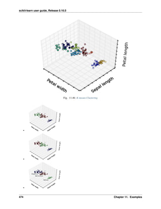
![scikit-learn user guide, Release 0.16.0
Python source code: plot_cluster_iris.py
print(__doc__)
# Code source: Gaël Varoquaux
# Modified for documentation by Jaques Grobler
# License: BSD 3 clause
import numpy as np
import matplotlib.pyplot as plt
from mpl_toolkits.mplot3d import Axes3D
from sklearn.cluster import KMeans
from sklearn import datasets
np.random.seed(5)
centers = [[1, 1], [-1, -1], [1, -1]]
iris = datasets.load_iris()
X = iris.data
y = iris.target
estimators = {'k_means_iris_3': KMeans(n_clusters=3),
'k_means_iris_8': KMeans(n_clusters=8),
'k_means_iris_bad_init': KMeans(n_clusters=3, n_init=1,
init='random')}
fignum = 1
for name, est in estimators.items():
fig = plt.figure(fignum, figsize=(4, 3))
plt.clf()
ax = Axes3D(fig, rect=[0, 0, .95, 1], elev=48, azim=134)
plt.cla()
est.fit(X)
labels = est.labels_
ax.scatter(X[:, 3], X[:, 0], X[:, 2], c=labels.astype(np.float))
ax.w_xaxis.set_ticklabels([])
ax.w_yaxis.set_ticklabels([])
ax.w_zaxis.set_ticklabels([])
ax.set_xlabel('Petal width')
ax.set_ylabel('Sepal length')
ax.set_zlabel('Petal length')
fignum = fignum + 1
# Plot the ground truth
fig = plt.figure(fignum, figsize=(4, 3))
plt.clf()
ax = Axes3D(fig, rect=[0, 0, .95, 1], elev=48, azim=134)
plt.cla()
for name, label in [('Setosa', 0),
('Versicolour', 1),
11.6. Clustering 475](https://image.slidesharecdn.com/scikit-learn0-150409112902-conversion-gate01/85/Scikit-learn-0-16-0-user-guide-485-320.jpg)
![scikit-learn user guide, Release 0.16.0
('Virginica', 2)]:
ax.text3D(X[y == label, 3].mean(),
X[y == label, 0].mean() + 1.5,
X[y == label, 2].mean(), name,
horizontalalignment='center',
bbox=dict(alpha=.5, edgecolor='w', facecolor='w'))
# Reorder the labels to have colors matching the cluster results
y = np.choose(y, [1, 2, 0]).astype(np.float)
ax.scatter(X[:, 3], X[:, 0], X[:, 2], c=y)
ax.w_xaxis.set_ticklabels([])
ax.w_yaxis.set_ticklabels([])
ax.w_zaxis.set_ticklabels([])
ax.set_xlabel('Petal width')
ax.set_ylabel('Sepal length')
ax.set_zlabel('Petal length')
plt.show()
Total running time of the example: 0.39 seconds ( 0 minutes 0.39 seconds)
Fig. 11.47: Various Agglomerative Clustering on a 2D embedding of digits
11.6.13 Various Agglomerative Clustering on a 2D embedding of digits
An illustration of various linkage option for agglomerative clustering on a 2D embedding of the digits dataset.
The goal of this example is to show intuitively how the metrics behave, and not to find good clusters for the digits.
This is why the example works on a 2D embedding.
What this example shows us is the behavior “rich getting richer” of agglomerative clustering that tends to create uneven
476 Chapter 11. Examples](https://image.slidesharecdn.com/scikit-learn0-150409112902-conversion-gate01/85/Scikit-learn-0-16-0-user-guide-486-320.jpg)

![scikit-learn user guide, Release 0.16.0
from scipy import ndimage
from matplotlib import pyplot as plt
from sklearn import manifold, datasets
digits = datasets.load_digits(n_class=10)
X = digits.data
y = digits.target
n_samples, n_features = X.shape
np.random.seed(0)
def nudge_images(X, y):
# Having a larger dataset shows more clearly the behavior of the
# methods, but we multiply the size of the dataset only by 2, as the
# cost of the hierarchical clustering methods are strongly
# super-linear in n_samples
shift = lambda x: ndimage.shift(x.reshape((8, 8)),
.3 * np.random.normal(size=2),
mode='constant',
).ravel()
X = np.concatenate([X, np.apply_along_axis(shift, 1, X)])
Y = np.concatenate([y, y], axis=0)
return X, Y
X, y = nudge_images(X, y)
#----------------------------------------------------------------------
# Visualize the clustering
def plot_clustering(X_red, X, labels, title=None):
x_min, x_max = np.min(X_red, axis=0), np.max(X_red, axis=0)
X_red = (X_red - x_min) / (x_max - x_min)
plt.figure(figsize=(6, 4))
for i in range(X_red.shape[0]):
plt.text(X_red[i, 0], X_red[i, 1], str(y[i]),
color=plt.cm.spectral(labels[i] / 10.),
fontdict={'weight': 'bold', 'size': 9})
plt.xticks([])
plt.yticks([])
if title is not None:
plt.title(title, size=17)
plt.axis('off')
plt.tight_layout()
#----------------------------------------------------------------------
# 2D embedding of the digits dataset
print("Computing embedding")
X_red = manifold.SpectralEmbedding(n_components=2).fit_transform(X)
print("Done.")
from sklearn.cluster import AgglomerativeClustering
for linkage in ('ward', 'average', 'complete'):
clustering = AgglomerativeClustering(linkage=linkage, n_clusters=10)
478 Chapter 11. Examples](https://image.slidesharecdn.com/scikit-learn0-150409112902-conversion-gate01/85/Scikit-learn-0-16-0-user-guide-488-320.jpg)


![scikit-learn user guide, Release 0.16.0
# License: BSD 3 clause
print(__doc__)
import numpy as np
import matplotlib.pyplot as plt
from sklearn.cluster import KMeans
from sklearn.metrics import pairwise_distances_argmin
from sklearn.datasets import load_sample_image
from sklearn.utils import shuffle
from time import time
n_colors = 64
# Load the Summer Palace photo
china = load_sample_image("china.jpg")
# Convert to floats instead of the default 8 bits integer coding. Dividing by
# 255 is important so that plt.imshow behaves works well on float data (need to
# be in the range [0-1]
china = np.array(china, dtype=np.float64) / 255
# Load Image and transform to a 2D numpy array.
w, h, d = original_shape = tuple(china.shape)
assert d == 3
image_array = np.reshape(china, (w * h, d))
print("Fitting model on a small sub-sample of the data")
t0 = time()
image_array_sample = shuffle(image_array, random_state=0)[:1000]
kmeans = KMeans(n_clusters=n_colors, random_state=0).fit(image_array_sample)
print("done in %0.3fs." % (time() - t0))
# Get labels for all points
print("Predicting color indices on the full image (k-means)")
t0 = time()
labels = kmeans.predict(image_array)
print("done in %0.3fs." % (time() - t0))
codebook_random = shuffle(image_array, random_state=0)[:n_colors + 1]
print("Predicting color indices on the full image (random)")
t0 = time()
labels_random = pairwise_distances_argmin(codebook_random,
image_array,
axis=0)
print("done in %0.3fs." % (time() - t0))
def recreate_image(codebook, labels, w, h):
"""Recreate the (compressed) image from the code book & labels"""
d = codebook.shape[1]
image = np.zeros((w, h, d))
label_idx = 0
for i in range(w):
for j in range(h):
image[i][j] = codebook[labels[label_idx]]
label_idx += 1
return image
11.6. Clustering 481](https://image.slidesharecdn.com/scikit-learn0-150409112902-conversion-gate01/85/Scikit-learn-0-16-0-user-guide-491-320.jpg)
![scikit-learn user guide, Release 0.16.0
# Display all results, alongside original image
plt.figure(1)
plt.clf()
ax = plt.axes([0, 0, 1, 1])
plt.axis('off')
plt.title('Original image (96,615 colors)')
plt.imshow(china)
plt.figure(2)
plt.clf()
ax = plt.axes([0, 0, 1, 1])
plt.axis('off')
plt.title('Quantized image (64 colors, K-Means)')
plt.imshow(recreate_image(kmeans.cluster_centers_, labels, w, h))
plt.figure(3)
plt.clf()
ax = plt.axes([0, 0, 1, 1])
plt.axis('off')
plt.title('Quantized image (64 colors, Random)')
plt.imshow(recreate_image(codebook_random, labels_random, w, h))
plt.show()
Total running time of the example: 1.51 seconds ( 0 minutes 1.51 seconds)
Fig. 11.49: Compare BIRCH and MiniBatchKMeans
482 Chapter 11. Examples](https://image.slidesharecdn.com/scikit-learn0-150409112902-conversion-gate01/85/Scikit-learn-0-16-0-user-guide-492-320.jpg)
![scikit-learn user guide, Release 0.16.0
11.6.15 Compare BIRCH and MiniBatchKMeans
This example compares the timing of Birch (with and without the global clustering step) and MiniBatchKMeans on a
synthetic dataset having 100,000 samples and 2 features generated using make_blobs.
If n_clusters is set to None, the data is reduced from 100,000 samples to a set of 158 clusters. This can be viewed
as a preprocessing step before the final (global) clustering step that further reduces these 158 clusters to 100 clusters.
Script output:
Birch without global clustering as the final step took 3.68 seconds
n_clusters : 158
Birch with global clustering as the final step took 3.65 seconds
n_clusters : 100
Time taken to run MiniBatchKMeans 4.84 seconds
Python source code: plot_birch_vs_minibatchkmeans.py
# Authors: Manoj Kumar <manojkumarsivaraj334@gmail.com
# Alexandre Gramfort <alexandre.gramfort@telecom-paristech.fr>
# License: BSD 3 clause
print(__doc__)
from itertools import cycle
from time import time
import numpy as np
import matplotlib.pyplot as plt
import matplotlib.colors as colors
from sklearn.preprocessing import StandardScaler
from sklearn.cluster import Birch, MiniBatchKMeans
from sklearn.datasets.samples_generator import make_blobs
# Generate centers for the blobs so that it forms a 10 X 10 grid.
xx = np.linspace(-22, 22, 10)
yy = np.linspace(-22, 22, 10)
xx, yy = np.meshgrid(xx, yy)
n_centres = np.hstack((np.ravel(xx)[:, np.newaxis],
np.ravel(yy)[:, np.newaxis]))
# Generate blobs to do a comparison between MiniBatchKMeans and Birch.
X, y = make_blobs(n_samples=100000, centers=n_centres, random_state=0)
11.6. Clustering 483](https://image.slidesharecdn.com/scikit-learn0-150409112902-conversion-gate01/85/Scikit-learn-0-16-0-user-guide-493-320.jpg)
![scikit-learn user guide, Release 0.16.0
# Use all colors that matplotlib provides by default.
colors_ = cycle(colors.cnames.keys())
fig = plt.figure(figsize=(12, 4))
fig.subplots_adjust(left=0.04, right=0.98, bottom=0.1, top=0.9)
# Compute clustering with Birch with and without the final clustering step
# and plot.
birch_models = [Birch(threshold=1.7, n_clusters=None),
Birch(threshold=1.7, n_clusters=100)]
final_step = ['without global clustering', 'with global clustering']
for ind, (birch_model, info) in enumerate(zip(birch_models, final_step)):
t = time()
birch_model.fit(X)
time_ = time() - t
print("Birch %s as the final step took %0.2f seconds" % (
info, (time() - t)))
# Plot result
labels = birch_model.labels_
centroids = birch_model.subcluster_centers_
n_clusters = np.unique(labels).size
print("n_clusters : %d" % n_clusters)
ax = fig.add_subplot(1, 3, ind + 1)
for this_centroid, k, col in zip(centroids, range(n_clusters), colors_):
mask = labels == k
ax.plot(X[mask, 0], X[mask, 1], 'w',
markerfacecolor=col, marker='.')
if birch_model.n_clusters is None:
ax.plot(this_centroid[0], this_centroid[1], '+', markerfacecolor=col,
markeredgecolor='k', markersize=5)
ax.set_ylim([-25, 25])
ax.set_xlim([-25, 25])
ax.set_autoscaley_on(False)
ax.set_title('Birch %s' % info)
# Compute clustering with MiniBatchKMeans.
mbk = MiniBatchKMeans(init='k-means++', n_clusters=100, batch_size=100,
n_init=10, max_no_improvement=10, verbose=0,
random_state=0)
t0 = time()
mbk.fit(X)
t_mini_batch = time() - t0
print("Time taken to run MiniBatchKMeans %0.2f seconds" % t_mini_batch)
mbk_means_labels_unique = np.unique(mbk.labels_)
ax = fig.add_subplot(1, 3, 3)
for this_centroid, k, col in zip(mbk.cluster_centers_,
range(n_clusters), colors_):
mask = mbk.labels_ == k
ax.plot(X[mask, 0], X[mask, 1], 'w', markerfacecolor=col, marker='.')
ax.plot(this_centroid[0], this_centroid[1], '+', markeredgecolor='k',
markersize=5)
ax.set_xlim([-25, 25])
ax.set_ylim([-25, 25])
ax.set_title("MiniBatchKMeans")
484 Chapter 11. Examples](https://image.slidesharecdn.com/scikit-learn0-150409112902-conversion-gate01/85/Scikit-learn-0-16-0-user-guide-494-320.jpg)
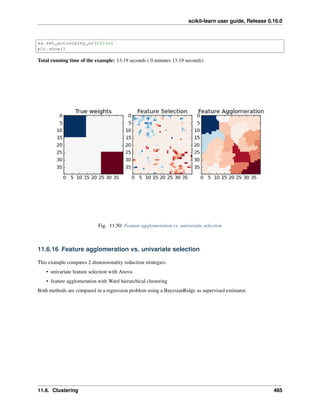
![scikit-learn user guide, Release 0.16.0
Script output:
________________________________________________________________________________
[Memory] Calling sklearn.cluster.hierarchical.ward_tree...
ward_tree(array([[-0.451933, ..., -0.675318],
...,
[ 0.275706, ..., -1.085711]]),
<1600x1600 sparse matrix of type '<type 'numpy.int64'>'
with 7840 stored elements in COOrdinate format>, n_components=None, n_clusters=None)
________________________________________________________ward_tree - 0.1s, 0.0min
________________________________________________________________________________
[Memory] Calling sklearn.cluster.hierarchical.ward_tree...
ward_tree(array([[ 0.905206, ..., 0.161245],
...,
[-0.849835, ..., -1.091621]]),
<1600x1600 sparse matrix of type '<type 'numpy.int64'>'
with 7840 stored elements in COOrdinate format>, n_components=None, n_clusters=None)
________________________________________________________ward_tree - 0.1s, 0.0min
________________________________________________________________________________
[Memory] Calling sklearn.cluster.hierarchical.ward_tree...
ward_tree(array([[ 0.905206, ..., -0.675318],
...,
[-0.849835, ..., -1.085711]]),
<1600x1600 sparse matrix of type '<type 'numpy.int64'>'
with 7840 stored elements in COOrdinate format>, n_components=None, n_clusters=None)
________________________________________________________ward_tree - 0.1s, 0.0min
________________________________________________________________________________
[Memory] Calling sklearn.feature_selection.univariate_selection.f_regression...
f_regression(array([[-0.451933, ..., 0.275706],
...,
[-0.675318, ..., -1.085711]]),
array([ 25.267703, ..., -25.026711]))
_____________________________________________________f_regression - 0.0s, 0.0min
________________________________________________________________________________
[Memory] Calling sklearn.feature_selection.univariate_selection.f_regression...
f_regression(array([[ 0.905206, ..., -0.849835],
...,
[ 0.161245, ..., -1.091621]]),
array([ -27.447268, ..., -112.638768]))
_____________________________________________________f_regression - 0.0s, 0.0min
________________________________________________________________________________
[Memory] Calling sklearn.feature_selection.univariate_selection.f_regression...
f_regression(array([[ 0.905206, ..., -0.849835],
486 Chapter 11. Examples](https://image.slidesharecdn.com/scikit-learn0-150409112902-conversion-gate01/85/Scikit-learn-0-16-0-user-guide-496-320.jpg)
![scikit-learn user guide, Release 0.16.0
...,
[-0.675318, ..., -1.085711]]),
array([-27.447268, ..., -25.026711]))
_____________________________________________________f_regression - 0.0s, 0.0min
Python source code: plot_feature_agglomeration_vs_univariate_selection.py
# Author: Alexandre Gramfort <alexandre.gramfort@inria.fr>
# License: BSD 3 clause
print(__doc__)
import shutil
import tempfile
import numpy as np
import matplotlib.pyplot as plt
from scipy import linalg, ndimage
from sklearn.feature_extraction.image import grid_to_graph
from sklearn import feature_selection
from sklearn.cluster import FeatureAgglomeration
from sklearn.linear_model import BayesianRidge
from sklearn.pipeline import Pipeline
from sklearn.grid_search import GridSearchCV
from sklearn.externals.joblib import Memory
from sklearn.cross_validation import KFold
###############################################################################
# Generate data
n_samples = 200
size = 40 # image size
roi_size = 15
snr = 5.
np.random.seed(0)
mask = np.ones([size, size], dtype=np.bool)
coef = np.zeros((size, size))
coef[0:roi_size, 0:roi_size] = -1.
coef[-roi_size:, -roi_size:] = 1.
X = np.random.randn(n_samples, size ** 2)
for x in X: # smooth data
x[:] = ndimage.gaussian_filter(x.reshape(size, size), sigma=1.0).ravel()
X -= X.mean(axis=0)
X /= X.std(axis=0)
y = np.dot(X, coef.ravel())
noise = np.random.randn(y.shape[0])
noise_coef = (linalg.norm(y, 2) / np.exp(snr / 20.)) / linalg.norm(noise, 2)
y += noise_coef * noise # add noise
###############################################################################
# Compute the coefs of a Bayesian Ridge with GridSearch
cv = KFold(len(y), 2) # cross-validation generator for model selection
ridge = BayesianRidge()
cachedir = tempfile.mkdtemp()
mem = Memory(cachedir=cachedir, verbose=1)
11.6. Clustering 487](https://image.slidesharecdn.com/scikit-learn0-150409112902-conversion-gate01/85/Scikit-learn-0-16-0-user-guide-497-320.jpg)
![scikit-learn user guide, Release 0.16.0
# Ward agglomeration followed by BayesianRidge
connectivity = grid_to_graph(n_x=size, n_y=size)
ward = FeatureAgglomeration(n_clusters=10, connectivity=connectivity,
memory=mem)
clf = Pipeline([('ward', ward), ('ridge', ridge)])
# Select the optimal number of parcels with grid search
clf = GridSearchCV(clf, {'ward__n_clusters': [10, 20, 30]}, n_jobs=1, cv=cv)
clf.fit(X, y) # set the best parameters
coef_ = clf.best_estimator_.steps[-1][1].coef_
coef_ = clf.best_estimator_.steps[0][1].inverse_transform(coef_)
coef_agglomeration_ = coef_.reshape(size, size)
# Anova univariate feature selection followed by BayesianRidge
f_regression = mem.cache(feature_selection.f_regression) # caching function
anova = feature_selection.SelectPercentile(f_regression)
clf = Pipeline([('anova', anova), ('ridge', ridge)])
# Select the optimal percentage of features with grid search
clf = GridSearchCV(clf, {'anova__percentile': [5, 10, 20]}, cv=cv)
clf.fit(X, y) # set the best parameters
coef_ = clf.best_estimator_.steps[-1][1].coef_
coef_ = clf.best_estimator_.steps[0][1].inverse_transform(coef_)
coef_selection_ = coef_.reshape(size, size)
###############################################################################
# Inverse the transformation to plot the results on an image
plt.close('all')
plt.figure(figsize=(7.3, 2.7))
plt.subplot(1, 3, 1)
plt.imshow(coef, interpolation="nearest", cmap=plt.cm.RdBu_r)
plt.title("True weights")
plt.subplot(1, 3, 2)
plt.imshow(coef_selection_, interpolation="nearest", cmap=plt.cm.RdBu_r)
plt.title("Feature Selection")
plt.subplot(1, 3, 3)
plt.imshow(coef_agglomeration_, interpolation="nearest", cmap=plt.cm.RdBu_r)
plt.title("Feature Agglomeration")
plt.subplots_adjust(0.04, 0.0, 0.98, 0.94, 0.16, 0.26)
plt.show()
# Attempt to remove the temporary cachedir, but don't worry if it fails
shutil.rmtree(cachedir, ignore_errors=True)
Total running time of the example: 1.61 seconds ( 0 minutes 1.61 seconds)
11.6.17 Agglomerative clustering with different metrics
Demonstrates the effect of different metrics on the hierarchical clustering.
The example is engineered to show the effect of the choice of different metrics. It is applied to waveforms, which
can be seen as high-dimensional vector. Indeed, the difference between metrics is usually more pronounced in high
dimension (in particular for euclidean and cityblock).
We generate data from three groups of waveforms. Two of the waveforms (waveform 1 and waveform 2) are propor-
tional one to the other. The cosine distance is invariant to a scaling of the data, as a result, it cannot distinguish these
two waveforms. Thus even with no noise, clustering using this distance will not separate out waveform 1 and 2.
We add observation noise to these waveforms. We generate very sparse noise: only 6% of the time points contain
noise. As a result, the l1 norm of this noise (ie “cityblock” distance) is much smaller than it’s l2 norm (“euclidean”
488 Chapter 11. Examples](https://image.slidesharecdn.com/scikit-learn0-150409112902-conversion-gate01/85/Scikit-learn-0-16-0-user-guide-498-320.jpg)


![scikit-learn user guide, Release 0.16.0
•
•
Python source code: plot_agglomerative_clustering_metrics.py
# Author: Gael Varoquaux
# License: BSD 3-Clause or CC-0
import matplotlib.pyplot as plt
import numpy as np
from sklearn.cluster import AgglomerativeClustering
from sklearn.metrics import pairwise_distances
np.random.seed(0)
# Generate waveform data
n_features = 2000
t = np.pi * np.linspace(0, 1, n_features)
def sqr(x):
return np.sign(np.cos(x))
X = list()
y = list()
for i, (phi, a) in enumerate([(.5, .15), (.5, .6), (.3, .2)]):
for _ in range(30):
phase_noise = .01 * np.random.normal()
amplitude_noise = .04 * np.random.normal()
additional_noise = 1 - 2 * np.random.rand(n_features)
# Make the noise sparse
11.6. Clustering 491](https://image.slidesharecdn.com/scikit-learn0-150409112902-conversion-gate01/85/Scikit-learn-0-16-0-user-guide-501-320.jpg)
![scikit-learn user guide, Release 0.16.0
additional_noise[np.abs(additional_noise) < .997] = 0
X.append(12 * ((a + amplitude_noise)
* (sqr(6 * (t + phi + phase_noise)))
+ additional_noise))
y.append(i)
X = np.array(X)
y = np.array(y)
n_clusters = 3
labels = ('Waveform 1', 'Waveform 2', 'Waveform 3')
# Plot the ground-truth labelling
plt.figure()
plt.axes([0, 0, 1, 1])
for l, c, n in zip(range(n_clusters), 'rgb',
labels):
lines = plt.plot(X[y == l].T, c=c, alpha=.5)
lines[0].set_label(n)
plt.legend(loc='best')
plt.axis('tight')
plt.axis('off')
plt.suptitle("Ground truth", size=20)
# Plot the distances
for index, metric in enumerate(["cosine", "euclidean", "cityblock"]):
avg_dist = np.zeros((n_clusters, n_clusters))
plt.figure(figsize=(5, 4.5))
for i in range(n_clusters):
for j in range(n_clusters):
avg_dist[i, j] = pairwise_distances(X[y == i], X[y == j],
metric=metric).mean()
avg_dist /= avg_dist.max()
for i in range(n_clusters):
for j in range(n_clusters):
plt.text(i, j, '%5.3f' % avg_dist[i, j],
verticalalignment='center',
horizontalalignment='center')
plt.imshow(avg_dist, interpolation='nearest', cmap=plt.cm.gnuplot2,
vmin=0)
plt.xticks(range(n_clusters), labels, rotation=45)
plt.yticks(range(n_clusters), labels)
plt.colorbar()
plt.suptitle("Interclass %s distances" % metric, size=18)
plt.tight_layout()
# Plot clustering results
for index, metric in enumerate(["cosine", "euclidean", "cityblock"]):
model = AgglomerativeClustering(n_clusters=n_clusters,
linkage="average", affinity=metric)
model.fit(X)
492 Chapter 11. Examples](https://image.slidesharecdn.com/scikit-learn0-150409112902-conversion-gate01/85/Scikit-learn-0-16-0-user-guide-502-320.jpg)
![scikit-learn user guide, Release 0.16.0
plt.figure()
plt.axes([0, 0, 1, 1])
for l, c in zip(np.arange(model.n_clusters), 'rgbk'):
plt.plot(X[model.labels_ == l].T, c=c, alpha=.5)
plt.axis('tight')
plt.axis('off')
plt.suptitle("AgglomerativeClustering(affinity=%s)" % metric, size=20)
plt.show()
Total running time of the example: 1.44 seconds ( 0 minutes 1.44 seconds)
Fig. 11.52: Empirical evaluation of the impact of k-means initialization
11.6.18 Empirical evaluation of the impact of k-means initialization
Evaluate the ability of k-means initializations strategies to make the algorithm convergence robust as measured by the
relative standard deviation of the inertia of the clustering (i.e. the sum of distances to the nearest cluster center).
The first plot shows the best inertia reached for each combination of the model (KMeans or MiniBatchKMeans)
and the init method (init="random" or init="kmeans++") for increasing values of the n_init parameter
that controls the number of initializations.
The second plot demonstrate one single run of the MiniBatchKMeans estimator using a init="random" and
n_init=1. This run leads to a bad convergence (local optimum) with estimated centers stuck between ground truth
clusters.
The dataset used for evaluation is a 2D grid of isotropic Gaussian clusters widely spaced.
11.6. Clustering 493](https://image.slidesharecdn.com/scikit-learn0-150409112902-conversion-gate01/85/Scikit-learn-0-16-0-user-guide-503-320.jpg)

![scikit-learn user guide, Release 0.16.0
# k-means models can do several random inits so as to be able to trade
# CPU time for convergence robustness
n_init_range = np.array([1, 5, 10, 15, 20])
# Datasets generation parameters
n_samples_per_center = 100
grid_size = 3
scale = 0.1
n_clusters = grid_size ** 2
def make_data(random_state, n_samples_per_center, grid_size, scale):
random_state = check_random_state(random_state)
centers = np.array([[i, j]
for i in range(grid_size)
for j in range(grid_size)])
n_clusters_true, n_features = centers.shape
noise = random_state.normal(
scale=scale, size=(n_samples_per_center, centers.shape[1]))
X = np.concatenate([c + noise for c in centers])
y = np.concatenate([[i] * n_samples_per_center
for i in range(n_clusters_true)])
return shuffle(X, y, random_state=random_state)
# Part 1: Quantitative evaluation of various init methods
fig = plt.figure()
plots = []
legends = []
cases = [
(KMeans, 'k-means++', {}),
(KMeans, 'random', {}),
(MiniBatchKMeans, 'k-means++', {'max_no_improvement': 3}),
(MiniBatchKMeans, 'random', {'max_no_improvement': 3, 'init_size': 500}),
]
for factory, init, params in cases:
print("Evaluation of %s with %s init" % (factory.__name__, init))
inertia = np.empty((len(n_init_range), n_runs))
for run_id in range(n_runs):
X, y = make_data(run_id, n_samples_per_center, grid_size, scale)
for i, n_init in enumerate(n_init_range):
km = factory(n_clusters=n_clusters, init=init, random_state=run_id,
n_init=n_init, **params).fit(X)
inertia[i, run_id] = km.inertia_
p = plt.errorbar(n_init_range, inertia.mean(axis=1), inertia.std(axis=1))
plots.append(p[0])
legends.append("%s with %s init" % (factory.__name__, init))
plt.xlabel('n_init')
plt.ylabel('inertia')
plt.legend(plots, legends)
plt.title("Mean inertia for various k-means init across %d runs" % n_runs)
11.6. Clustering 495](https://image.slidesharecdn.com/scikit-learn0-150409112902-conversion-gate01/85/Scikit-learn-0-16-0-user-guide-505-320.jpg)
![scikit-learn user guide, Release 0.16.0
# Part 2: Qualitative visual inspection of the convergence
X, y = make_data(random_state, n_samples_per_center, grid_size, scale)
km = MiniBatchKMeans(n_clusters=n_clusters, init='random', n_init=1,
random_state=random_state).fit(X)
fig = plt.figure()
for k in range(n_clusters):
my_members = km.labels_ == k
color = cm.spectral(float(k) / n_clusters, 1)
plt.plot(X[my_members, 0], X[my_members, 1], 'o', marker='.', c=color)
cluster_center = km.cluster_centers_[k]
plt.plot(cluster_center[0], cluster_center[1], 'o',
markerfacecolor=color, markeredgecolor='k', markersize=6)
plt.title("Example cluster allocation with a single random initn"
"with MiniBatchKMeans")
plt.show()
Total running time of the example: 3.16 seconds ( 0 minutes 3.16 seconds)
Fig. 11.53: A demo of K-Means clustering on the handwritten digits data
11.6.19 A demo of K-Means clustering on the handwritten digits data
In this example we compare the various initialization strategies for K-means in terms of runtime and quality of the
results.
As the ground truth is known here, we also apply different cluster quality metrics to judge the goodness of fit of the
cluster labels to the ground truth.
496 Chapter 11. Examples](https://image.slidesharecdn.com/scikit-learn0-150409112902-conversion-gate01/85/Scikit-learn-0-16-0-user-guide-506-320.jpg)


![scikit-learn user guide, Release 0.16.0
# Visualize the results on PCA-reduced data
reduced_data = PCA(n_components=2).fit_transform(data)
kmeans = KMeans(init='k-means++', n_clusters=n_digits, n_init=10)
kmeans.fit(reduced_data)
# Step size of the mesh. Decrease to increase the quality of the VQ.
h = .02 # point in the mesh [x_min, m_max]x[y_min, y_max].
# Plot the decision boundary. For that, we will assign a color to each
x_min, x_max = reduced_data[:, 0].min() + 1, reduced_data[:, 0].max() - 1
y_min, y_max = reduced_data[:, 1].min() + 1, reduced_data[:, 1].max() - 1
xx, yy = np.meshgrid(np.arange(x_min, x_max, h), np.arange(y_min, y_max, h))
# Obtain labels for each point in mesh. Use last trained model.
Z = kmeans.predict(np.c_[xx.ravel(), yy.ravel()])
# Put the result into a color plot
Z = Z.reshape(xx.shape)
plt.figure(1)
plt.clf()
plt.imshow(Z, interpolation='nearest',
extent=(xx.min(), xx.max(), yy.min(), yy.max()),
cmap=plt.cm.Paired,
aspect='auto', origin='lower')
plt.plot(reduced_data[:, 0], reduced_data[:, 1], 'k.', markersize=2)
# Plot the centroids as a white X
centroids = kmeans.cluster_centers_
plt.scatter(centroids[:, 0], centroids[:, 1],
marker='x', s=169, linewidths=3,
color='w', zorder=10)
plt.title('K-means clustering on the digits dataset (PCA-reduced data)n'
'Centroids are marked with white cross')
plt.xlim(x_min, x_max)
plt.ylim(y_min, y_max)
plt.xticks(())
plt.yticks(())
plt.show()
Total running time of the example: 2.35 seconds ( 0 minutes 2.35 seconds)
11.6.20 Adjustment for chance in clustering performance evaluation
The following plots demonstrate the impact of the number of clusters and number of samples on various clustering
performance evaluation metrics.
Non-adjusted measures such as the V-Measure show a dependency between the number of clusters and the number of
samples: the mean V-Measure of random labeling increases significantly as the number of clusters is closer to the total
number of samples used to compute the measure.
Adjusted for chance measure such as ARI display some random variations centered around a mean score of 0.0 for
any number of samples and clusters.
Only adjusted measures can hence safely be used as a consensus index to evaluate the average stability of clustering
algorithms for a given value of k on various overlapping sub-samples of the dataset.
11.6. Clustering 499](https://image.slidesharecdn.com/scikit-learn0-150409112902-conversion-gate01/85/Scikit-learn-0-16-0-user-guide-509-320.jpg)

![scikit-learn user guide, Release 0.16.0
Script output:
Computing adjusted_rand_score for 10 values of n_clusters and n_samples=100
done in 0.101s
Computing v_measure_score for 10 values of n_clusters and n_samples=100
done in 0.028s
Computing adjusted_mutual_info_score for 10 values of n_clusters and n_samples=100
done in 0.559s
Computing mutual_info_score for 10 values of n_clusters and n_samples=100
done in 0.023s
Computing adjusted_rand_score for 10 values of n_clusters and n_samples=1000
done in 0.072s
Computing v_measure_score for 10 values of n_clusters and n_samples=1000
done in 0.063s
Computing adjusted_mutual_info_score for 10 values of n_clusters and n_samples=1000
done in 0.343s
Computing mutual_info_score for 10 values of n_clusters and n_samples=1000
done in 0.040s
Python source code: plot_adjusted_for_chance_measures.py
print(__doc__)
# Author: Olivier Grisel <olivier.grisel@ensta.org>
# License: BSD 3 clause
import numpy as np
import matplotlib.pyplot as plt
from time import time
from sklearn import metrics
def uniform_labelings_scores(score_func, n_samples, n_clusters_range,
fixed_n_classes=None, n_runs=5, seed=42):
"""Compute score for 2 random uniform cluster labelings.
Both random labelings have the same number of clusters for each value
possible value in ``n_clusters_range``.
When fixed_n_classes is not None the first labeling is considered a ground
truth class assignment with fixed number of classes.
"""
random_labels = np.random.RandomState(seed).random_integers
scores = np.zeros((len(n_clusters_range), n_runs))
if fixed_n_classes is not None:
labels_a = random_labels(low=0, high=fixed_n_classes - 1,
size=n_samples)
for i, k in enumerate(n_clusters_range):
for j in range(n_runs):
if fixed_n_classes is None:
labels_a = random_labels(low=0, high=k - 1, size=n_samples)
labels_b = random_labels(low=0, high=k - 1, size=n_samples)
scores[i, j] = score_func(labels_a, labels_b)
return scores
score_funcs = [
metrics.adjusted_rand_score,
11.6. Clustering 501](https://image.slidesharecdn.com/scikit-learn0-150409112902-conversion-gate01/85/Scikit-learn-0-16-0-user-guide-511-320.jpg)
![scikit-learn user guide, Release 0.16.0
metrics.v_measure_score,
metrics.adjusted_mutual_info_score,
metrics.mutual_info_score,
]
# 2 independent random clusterings with equal cluster number
n_samples = 100
n_clusters_range = np.linspace(2, n_samples, 10).astype(np.int)
plt.figure(1)
plots = []
names = []
for score_func in score_funcs:
print("Computing %s for %d values of n_clusters and n_samples=%d"
% (score_func.__name__, len(n_clusters_range), n_samples))
t0 = time()
scores = uniform_labelings_scores(score_func, n_samples, n_clusters_range)
print("done in %0.3fs" % (time() - t0))
plots.append(plt.errorbar(
n_clusters_range, np.median(scores, axis=1), scores.std(axis=1))[0])
names.append(score_func.__name__)
plt.title("Clustering measures for 2 random uniform labelingsn"
"with equal number of clusters")
plt.xlabel('Number of clusters (Number of samples is fixed to %d)' % n_samples)
plt.ylabel('Score value')
plt.legend(plots, names)
plt.ylim(ymin=-0.05, ymax=1.05)
# Random labeling with varying n_clusters against ground class labels
# with fixed number of clusters
n_samples = 1000
n_clusters_range = np.linspace(2, 100, 10).astype(np.int)
n_classes = 10
plt.figure(2)
plots = []
names = []
for score_func in score_funcs:
print("Computing %s for %d values of n_clusters and n_samples=%d"
% (score_func.__name__, len(n_clusters_range), n_samples))
t0 = time()
scores = uniform_labelings_scores(score_func, n_samples, n_clusters_range,
fixed_n_classes=n_classes)
print("done in %0.3fs" % (time() - t0))
plots.append(plt.errorbar(
n_clusters_range, scores.mean(axis=1), scores.std(axis=1))[0])
names.append(score_func.__name__)
plt.title("Clustering measures for random uniform labelingn"
"against reference assignment with %d classes" % n_classes)
502 Chapter 11. Examples](https://image.slidesharecdn.com/scikit-learn0-150409112902-conversion-gate01/85/Scikit-learn-0-16-0-user-guide-512-320.jpg)

![scikit-learn user guide, Release 0.16.0
Python source code: plot_cluster_comparison.py
print(__doc__)
import time
import numpy as np
import matplotlib.pyplot as plt
from sklearn import cluster, datasets
from sklearn.neighbors import kneighbors_graph
from sklearn.preprocessing import StandardScaler
np.random.seed(0)
# Generate datasets. We choose the size big enough to see the scalability
# of the algorithms, but not too big to avoid too long running times
n_samples = 1500
noisy_circles = datasets.make_circles(n_samples=n_samples, factor=.5,
noise=.05)
noisy_moons = datasets.make_moons(n_samples=n_samples, noise=.05)
blobs = datasets.make_blobs(n_samples=n_samples, random_state=8)
no_structure = np.random.rand(n_samples, 2), None
colors = np.array([x for x in 'bgrcmykbgrcmykbgrcmykbgrcmyk'])
colors = np.hstack([colors] * 20)
clustering_names = [
'MiniBatchKMeans', 'AffinityPropagation', 'MeanShift',
'SpectralClustering', 'Ward', 'AgglomerativeClustering',
'DBSCAN', 'Birch']
plt.figure(figsize=(len(clustering_names) * 2 + 3, 9.5))
plt.subplots_adjust(left=.02, right=.98, bottom=.001, top=.96, wspace=.05,
hspace=.01)
plot_num = 1
504 Chapter 11. Examples](https://image.slidesharecdn.com/scikit-learn0-150409112902-conversion-gate01/85/Scikit-learn-0-16-0-user-guide-514-320.jpg)
![scikit-learn user guide, Release 0.16.0
datasets = [noisy_circles, noisy_moons, blobs, no_structure]
for i_dataset, dataset in enumerate(datasets):
X, y = dataset
# normalize dataset for easier parameter selection
X = StandardScaler().fit_transform(X)
# estimate bandwidth for mean shift
bandwidth = cluster.estimate_bandwidth(X, quantile=0.3)
# connectivity matrix for structured Ward
connectivity = kneighbors_graph(X, n_neighbors=10, include_self=False)
# make connectivity symmetric
connectivity = 0.5 * (connectivity + connectivity.T)
# create clustering estimators
ms = cluster.MeanShift(bandwidth=bandwidth, bin_seeding=True)
two_means = cluster.MiniBatchKMeans(n_clusters=2)
ward = cluster.AgglomerativeClustering(n_clusters=2, linkage='ward',
connectivity=connectivity)
spectral = cluster.SpectralClustering(n_clusters=2,
eigen_solver='arpack',
affinity="nearest_neighbors")
dbscan = cluster.DBSCAN(eps=.2)
affinity_propagation = cluster.AffinityPropagation(damping=.9,
preference=-200)
average_linkage = cluster.AgglomerativeClustering(
linkage="average", affinity="cityblock", n_clusters=2,
connectivity=connectivity)
birch = cluster.Birch(n_clusters=2)
clustering_algorithms = [
two_means, affinity_propagation, ms, spectral, ward, average_linkage,
dbscan, birch]
for name, algorithm in zip(clustering_names, clustering_algorithms):
# predict cluster memberships
t0 = time.time()
algorithm.fit(X)
t1 = time.time()
if hasattr(algorithm, 'labels_'):
y_pred = algorithm.labels_.astype(np.int)
else:
y_pred = algorithm.predict(X)
# plot
plt.subplot(4, len(clustering_algorithms), plot_num)
if i_dataset == 0:
plt.title(name, size=18)
plt.scatter(X[:, 0], X[:, 1], color=colors[y_pred].tolist(), s=10)
if hasattr(algorithm, 'cluster_centers_'):
centers = algorithm.cluster_centers_
center_colors = colors[:len(centers)]
plt.scatter(centers[:, 0], centers[:, 1], s=100, c=center_colors)
plt.xlim(-2, 2)
plt.ylim(-2, 2)
plt.xticks(())
11.6. Clustering 505](https://image.slidesharecdn.com/scikit-learn0-150409112902-conversion-gate01/85/Scikit-learn-0-16-0-user-guide-515-320.jpg)

![scikit-learn user guide, Release 0.16.0
Python source code: plot_mini_batch_kmeans.py
print(__doc__)
import time
import numpy as np
import matplotlib.pyplot as plt
from sklearn.cluster import MiniBatchKMeans, KMeans
from sklearn.metrics.pairwise import pairwise_distances_argmin
from sklearn.datasets.samples_generator import make_blobs
##############################################################################
# Generate sample data
np.random.seed(0)
batch_size = 45
centers = [[1, 1], [-1, -1], [1, -1]]
n_clusters = len(centers)
X, labels_true = make_blobs(n_samples=3000, centers=centers, cluster_std=0.7)
##############################################################################
# Compute clustering with Means
k_means = KMeans(init='k-means++', n_clusters=3, n_init=10)
t0 = time.time()
k_means.fit(X)
t_batch = time.time() - t0
k_means_labels = k_means.labels_
k_means_cluster_centers = k_means.cluster_centers_
k_means_labels_unique = np.unique(k_means_labels)
##############################################################################
# Compute clustering with MiniBatchKMeans
mbk = MiniBatchKMeans(init='k-means++', n_clusters=3, batch_size=batch_size,
n_init=10, max_no_improvement=10, verbose=0)
t0 = time.time()
mbk.fit(X)
t_mini_batch = time.time() - t0
mbk_means_labels = mbk.labels_
11.6. Clustering 507](https://image.slidesharecdn.com/scikit-learn0-150409112902-conversion-gate01/85/Scikit-learn-0-16-0-user-guide-517-320.jpg)
![scikit-learn user guide, Release 0.16.0
mbk_means_cluster_centers = mbk.cluster_centers_
mbk_means_labels_unique = np.unique(mbk_means_labels)
##############################################################################
# Plot result
fig = plt.figure(figsize=(8, 3))
fig.subplots_adjust(left=0.02, right=0.98, bottom=0.05, top=0.9)
colors = ['#4EACC5', '#FF9C34', '#4E9A06']
# We want to have the same colors for the same cluster from the
# MiniBatchKMeans and the KMeans algorithm. Let's pair the cluster centers per
# closest one.
order = pairwise_distances_argmin(k_means_cluster_centers,
mbk_means_cluster_centers)
# KMeans
ax = fig.add_subplot(1, 3, 1)
for k, col in zip(range(n_clusters), colors):
my_members = k_means_labels == k
cluster_center = k_means_cluster_centers[k]
ax.plot(X[my_members, 0], X[my_members, 1], 'w',
markerfacecolor=col, marker='.')
ax.plot(cluster_center[0], cluster_center[1], 'o', markerfacecolor=col,
markeredgecolor='k', markersize=6)
ax.set_title('KMeans')
ax.set_xticks(())
ax.set_yticks(())
plt.text(-3.5, 1.8, 'train time: %.2fsninertia: %f' % (
t_batch, k_means.inertia_))
# MiniBatchKMeans
ax = fig.add_subplot(1, 3, 2)
for k, col in zip(range(n_clusters), colors):
my_members = mbk_means_labels == order[k]
cluster_center = mbk_means_cluster_centers[order[k]]
ax.plot(X[my_members, 0], X[my_members, 1], 'w',
markerfacecolor=col, marker='.')
ax.plot(cluster_center[0], cluster_center[1], 'o', markerfacecolor=col,
markeredgecolor='k', markersize=6)
ax.set_title('MiniBatchKMeans')
ax.set_xticks(())
ax.set_yticks(())
plt.text(-3.5, 1.8, 'train time: %.2fsninertia: %f' %
(t_mini_batch, mbk.inertia_))
# Initialise the different array to all False
different = (mbk_means_labels == 4)
ax = fig.add_subplot(1, 3, 3)
for l in range(n_clusters):
different += ((k_means_labels == k) != (mbk_means_labels == order[k]))
identic = np.logical_not(different)
ax.plot(X[identic, 0], X[identic, 1], 'w',
markerfacecolor='#bbbbbb', marker='.')
ax.plot(X[different, 0], X[different, 1], 'w',
508 Chapter 11. Examples](https://image.slidesharecdn.com/scikit-learn0-150409112902-conversion-gate01/85/Scikit-learn-0-16-0-user-guide-518-320.jpg)
![scikit-learn user guide, Release 0.16.0
markerfacecolor='m', marker='.')
ax.set_title('Difference')
ax.set_xticks(())
ax.set_yticks(())
plt.show()
Total running time of the example: 0.20 seconds ( 0 minutes 0.20 seconds)
Fig. 11.57: Selecting the number of clusters with silhouette analysis on KMeans clustering
11.6.23 Selecting the number of clusters with silhouette analysis on KMeans clus-
tering
Silhouette analysis can be used to study the separation distance between the resulting clusters. The silhouette plot
displays a measure of how close each point in one cluster is to points in the neighboring clusters and thus provides a
way to assess parameters like number of clusters visually. This measure has a range of [-1, 1].
Silhoette coefficients (as these values are referred to as) near +1 indicate that the sample is far away from the neigh-
boring clusters. A value of 0 indicates that the sample is on or very close to the decision boundary between two
neighboring clusters and negative values indicate that those samples might have been assigned to the wrong cluster.
In this example the silhouette analysis is used to choose an optimal value for n_clusters. The silhouette plot shows
that the n_clusters value of 3, 5 and 6 are a bad pick for the given data due to the presence of clusters with below
average silhouette scores and also due to wide fluctuations in the size of the silhouette plots. Silhouette analysis is
more ambivalent in deciding between 2 and 4.
Also from the thickness of the silhouette plot the cluster size can be visualized. The silhouette plot for cluster 0 when
n_clusters is equal to 2, is bigger in size owing to the grouping of the 3 sub clusters into one big cluster. However
11.6. Clustering 509](https://image.slidesharecdn.com/scikit-learn0-150409112902-conversion-gate01/85/Scikit-learn-0-16-0-user-guide-519-320.jpg)

![scikit-learn user guide, Release 0.16.0
import matplotlib.pyplot as plt
import matplotlib.cm as cm
import numpy as np
print(__doc__)
# Generating the sample data from make_blobs
# This particular setting has one distict cluster and 3 clusters placed close
# together.
X, y = make_blobs(n_samples=500,
n_features=2,
centers=4,
cluster_std=1,
center_box=(-10.0, 10.0),
shuffle=True,
random_state=1) # For reproducibility
range_n_clusters = [2, 3, 4, 5, 6]
for n_clusters in range_n_clusters:
# Create a subplot with 1 row and 2 columns
fig, (ax1, ax2) = plt.subplots(1, 2)
fig.set_size_inches(18, 7)
# The 1st subplot is the silhouette plot
# The silhouette coefficient can range from -1, 1 but in this example all
# lie within [-0.1, 1]
ax1.set_xlim([-0.1, 1])
# The (n_clusters+1)*10 is for inserting blank space between silhouette
# plots of individual clusters, to demarcate them clearly.
ax1.set_ylim([0, len(X) + (n_clusters + 1) * 10])
# Initialize the clusterer with n_clusters value and a random generator
# seed of 10 for reproducibility.
clusterer = KMeans(n_clusters=n_clusters, random_state=10)
cluster_labels = clusterer.fit_predict(X)
# The silhouette_score gives the average value for all the samples.
# This gives a perspective into the density and separation of the formed
# clusters
silhouette_avg = silhouette_score(X, cluster_labels)
print("For n_clusters =", n_clusters,
"The average silhouette_score is :", silhouette_avg)
# Compute the silhouette scores for each sample
sample_silhouette_values = silhouette_samples(X, cluster_labels)
y_lower = 10
for i in range(n_clusters):
# Aggregate the silhouette scores for samples belonging to
# cluster i, and sort them
ith_cluster_silhouette_values =
sample_silhouette_values[cluster_labels == i]
ith_cluster_silhouette_values.sort()
size_cluster_i = ith_cluster_silhouette_values.shape[0]
y_upper = y_lower + size_cluster_i
11.6. Clustering 511](https://image.slidesharecdn.com/scikit-learn0-150409112902-conversion-gate01/85/Scikit-learn-0-16-0-user-guide-521-320.jpg)
![scikit-learn user guide, Release 0.16.0
color = cm.spectral(float(i) / n_clusters)
ax1.fill_betweenx(np.arange(y_lower, y_upper),
0, ith_cluster_silhouette_values,
facecolor=color, edgecolor=color, alpha=0.7)
# Label the silhouette plots with their cluster numbers at the middle
ax1.text(-0.05, y_lower + 0.5 * size_cluster_i, str(i))
# Compute the new y_lower for next plot
y_lower = y_upper + 10 # 10 for the 0 samples
ax1.set_title("The silhouette plot for the various clusters.")
ax1.set_xlabel("The silhouette coefficient values")
ax1.set_ylabel("Cluster label")
# The vertical line for average silhoutte score of all the values
ax1.axvline(x=silhouette_avg, color="red", linestyle="--")
ax1.set_yticks([]) # Clear the yaxis labels / ticks
ax1.set_xticks([-0.1, 0, 0.2, 0.4, 0.6, 0.8, 1])
# 2nd Plot showing the actual clusters formed
colors = cm.spectral(cluster_labels.astype(float) / n_clusters)
ax2.scatter(X[:, 0], X[:, 1], marker='.', s=30, lw=0, alpha=0.7,
c=colors)
# Labeling the clusters
centers = clusterer.cluster_centers_
# Draw white circles at cluster centers
ax2.scatter(centers[:, 0], centers[:, 1],
marker='o', c="white", alpha=1, s=200)
for i, c in enumerate(centers):
ax2.scatter(c[0], c[1], marker='$%d$' % i, alpha=1, s=50)
ax2.set_title("The visualization of the clustered data.")
ax2.set_xlabel("Feature space for the 1st feature")
ax2.set_ylabel("Feature space for the 2nd feature")
plt.suptitle(("Silhouette analysis for KMeans clustering on sample data "
"with n_clusters = %d" % n_clusters),
fontsize=14, fontweight='bold')
plt.show()
Total running time of the example: 1.51 seconds ( 0 minutes 1.51 seconds)
11.7 Covariance estimation
Examples concerning the sklearn.covariance module.
512 Chapter 11. Examples](https://image.slidesharecdn.com/scikit-learn0-150409112902-conversion-gate01/85/Scikit-learn-0-16-0-user-guide-522-320.jpg)
![scikit-learn user guide, Release 0.16.0
Fig. 11.58: Ledoit-Wolf vs OAS estimation
11.7.1 Ledoit-Wolf vs OAS estimation
The usual covariance maximum likelihood estimate can be regularized using shrinkage. Ledoit and Wolf proposed a
close formula to compute the asymptotically optimal shrinkage parameter (minimizing a MSE criterion), yielding the
Ledoit-Wolf covariance estimate.
Chen et al. proposed an improvement of the Ledoit-Wolf shrinkage parameter, the OAS coefficient, whose convergence
is significantly better under the assumption that the data are Gaussian.
This example, inspired from Chen’s publication [1], shows a comparison of the estimated MSE of the LW and OAS
methods, using Gaussian distributed data.
[1] “Shrinkage Algorithms for MMSE Covariance Estimation” Chen et al., IEEE Trans. on Sign. Proc., Volume 58,
Issue 10, October 2010.
11.7. Covariance estimation 513](https://image.slidesharecdn.com/scikit-learn0-150409112902-conversion-gate01/85/Scikit-learn-0-16-0-user-guide-523-320.jpg)

![scikit-learn user guide, Release 0.16.0
X = np.dot(
np.random.normal(size=(n_samples, n_features)), coloring_matrix.T)
lw = LedoitWolf(store_precision=False, assume_centered=True)
lw.fit(X)
lw_mse[i, j] = lw.error_norm(real_cov, scaling=False)
lw_shrinkage[i, j] = lw.shrinkage_
oa = OAS(store_precision=False, assume_centered=True)
oa.fit(X)
oa_mse[i, j] = oa.error_norm(real_cov, scaling=False)
oa_shrinkage[i, j] = oa.shrinkage_
# plot MSE
plt.subplot(2, 1, 1)
plt.errorbar(n_samples_range, lw_mse.mean(1), yerr=lw_mse.std(1),
label='Ledoit-Wolf', color='g')
plt.errorbar(n_samples_range, oa_mse.mean(1), yerr=oa_mse.std(1),
label='OAS', color='r')
plt.ylabel("Squared error")
plt.legend(loc="upper right")
plt.title("Comparison of covariance estimators")
plt.xlim(5, 31)
# plot shrinkage coefficient
plt.subplot(2, 1, 2)
plt.errorbar(n_samples_range, lw_shrinkage.mean(1), yerr=lw_shrinkage.std(1),
label='Ledoit-Wolf', color='g')
plt.errorbar(n_samples_range, oa_shrinkage.mean(1), yerr=oa_shrinkage.std(1),
label='OAS', color='r')
plt.xlabel("n_samples")
plt.ylabel("Shrinkage")
plt.legend(loc="lower right")
plt.ylim(plt.ylim()[0], 1. + (plt.ylim()[1] - plt.ylim()[0]) / 10.)
plt.xlim(5, 31)
plt.show()
Total running time of the example: 4.21 seconds ( 0 minutes 4.21 seconds)
11.7.2 Outlier detection with several methods.
When the amount of contamination is known, this example illustrates two different ways of performing Novelty and
Outlier Detection:
• based on a robust estimator of covariance, which is assuming that the data are Gaussian distributed and performs
better than the One-Class SVM in that case.
• using the One-Class SVM and its ability to capture the shape of the data set, hence performing better when the
data is strongly non-Gaussian, i.e. with two well-separated clusters;
The ground truth about inliers and outliers is given by the points colors while the orange-filled area indicates which
points are reported as inliers by each method.
Here, we assume that we know the fraction of outliers in the datasets. Thus rather than using the ‘predict’ method of
the objects, we set the threshold on the decision_function to separate out the corresponding fraction.
11.7. Covariance estimation 515](https://image.slidesharecdn.com/scikit-learn0-150409112902-conversion-gate01/85/Scikit-learn-0-16-0-user-guide-525-320.jpg)
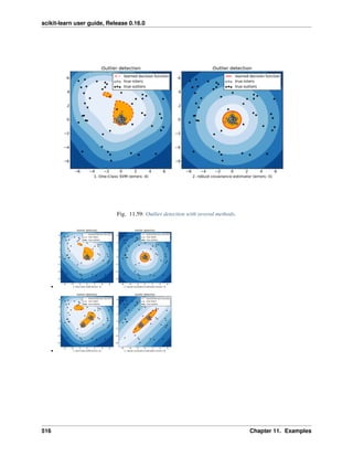
![scikit-learn user guide, Release 0.16.0
•
Python source code: plot_outlier_detection.py
print(__doc__)
import numpy as np
import matplotlib.pyplot as plt
import matplotlib.font_manager
from scipy import stats
from sklearn import svm
from sklearn.covariance import EllipticEnvelope
# Example settings
n_samples = 200
outliers_fraction = 0.25
clusters_separation = [0, 1, 2]
# define two outlier detection tools to be compared
classifiers = {
"One-Class SVM": svm.OneClassSVM(nu=0.95 * outliers_fraction + 0.05,
kernel="rbf", gamma=0.1),
"robust covariance estimator": EllipticEnvelope(contamination=.1)}
# Compare given classifiers under given settings
xx, yy = np.meshgrid(np.linspace(-7, 7, 500), np.linspace(-7, 7, 500))
n_inliers = int((1. - outliers_fraction) * n_samples)
n_outliers = int(outliers_fraction * n_samples)
ground_truth = np.ones(n_samples, dtype=int)
ground_truth[-n_outliers:] = 0
# Fit the problem with varying cluster separation
for i, offset in enumerate(clusters_separation):
np.random.seed(42)
# Data generation
X1 = 0.3 * np.random.randn(0.5 * n_inliers, 2) - offset
X2 = 0.3 * np.random.randn(0.5 * n_inliers, 2) + offset
X = np.r_[X1, X2]
# Add outliers
X = np.r_[X, np.random.uniform(low=-6, high=6, size=(n_outliers, 2))]
# Fit the model with the One-Class SVM
plt.figure(figsize=(10, 5))
for i, (clf_name, clf) in enumerate(classifiers.items()):
# fit the data and tag outliers
clf.fit(X)
y_pred = clf.decision_function(X).ravel()
threshold = stats.scoreatpercentile(y_pred,
100 * outliers_fraction)
y_pred = y_pred > threshold
11.7. Covariance estimation 517](https://image.slidesharecdn.com/scikit-learn0-150409112902-conversion-gate01/85/Scikit-learn-0-16-0-user-guide-527-320.jpg)
![scikit-learn user guide, Release 0.16.0
n_errors = (y_pred != ground_truth).sum()
# plot the levels lines and the points
Z = clf.decision_function(np.c_[xx.ravel(), yy.ravel()])
Z = Z.reshape(xx.shape)
subplot = plt.subplot(1, 2, i + 1)
subplot.set_title("Outlier detection")
subplot.contourf(xx, yy, Z, levels=np.linspace(Z.min(), threshold, 7),
cmap=plt.cm.Blues_r)
a = subplot.contour(xx, yy, Z, levels=[threshold],
linewidths=2, colors='red')
subplot.contourf(xx, yy, Z, levels=[threshold, Z.max()],
colors='orange')
b = subplot.scatter(X[:-n_outliers, 0], X[:-n_outliers, 1], c='white')
c = subplot.scatter(X[-n_outliers:, 0], X[-n_outliers:, 1], c='black')
subplot.axis('tight')
subplot.legend(
[a.collections[0], b, c],
['learned decision function', 'true inliers', 'true outliers'],
prop=matplotlib.font_manager.FontProperties(size=11))
subplot.set_xlabel("%d. %s (errors: %d)" % (i + 1, clf_name, n_errors))
subplot.set_xlim((-7, 7))
subplot.set_ylim((-7, 7))
plt.subplots_adjust(0.04, 0.1, 0.96, 0.94, 0.1, 0.26)
plt.show()
Total running time of the example: 1.87 seconds ( 0 minutes 1.87 seconds)
Fig. 11.60: Sparse inverse covariance estimation
518 Chapter 11. Examples](https://image.slidesharecdn.com/scikit-learn0-150409112902-conversion-gate01/85/Scikit-learn-0-16-0-user-guide-528-320.jpg)

![scikit-learn user guide, Release 0.16.0
# License: BSD 3 clause
# Copyright: INRIA
import numpy as np
from scipy import linalg
from sklearn.datasets import make_sparse_spd_matrix
from sklearn.covariance import GraphLassoCV, ledoit_wolf
import matplotlib.pyplot as plt
##############################################################################
# Generate the data
n_samples = 60
n_features = 20
prng = np.random.RandomState(1)
prec = make_sparse_spd_matrix(n_features, alpha=.98,
smallest_coef=.4,
largest_coef=.7,
random_state=prng)
cov = linalg.inv(prec)
d = np.sqrt(np.diag(cov))
cov /= d
cov /= d[:, np.newaxis]
prec *= d
prec *= d[:, np.newaxis]
X = prng.multivariate_normal(np.zeros(n_features), cov, size=n_samples)
X -= X.mean(axis=0)
X /= X.std(axis=0)
##############################################################################
# Estimate the covariance
emp_cov = np.dot(X.T, X) / n_samples
model = GraphLassoCV()
model.fit(X)
cov_ = model.covariance_
prec_ = model.precision_
lw_cov_, _ = ledoit_wolf(X)
lw_prec_ = linalg.inv(lw_cov_)
##############################################################################
# Plot the results
plt.figure(figsize=(10, 6))
plt.subplots_adjust(left=0.02, right=0.98)
# plot the covariances
covs = [('Empirical', emp_cov), ('Ledoit-Wolf', lw_cov_),
('GraphLasso', cov_), ('True', cov)]
vmax = cov_.max()
for i, (name, this_cov) in enumerate(covs):
plt.subplot(2, 4, i + 1)
plt.imshow(this_cov, interpolation='nearest', vmin=-vmax, vmax=vmax,
cmap=plt.cm.RdBu_r)
plt.xticks(())
plt.yticks(())
plt.title('%s covariance' % name)
520 Chapter 11. Examples](https://image.slidesharecdn.com/scikit-learn0-150409112902-conversion-gate01/85/Scikit-learn-0-16-0-user-guide-530-320.jpg)
![scikit-learn user guide, Release 0.16.0
# plot the precisions
precs = [('Empirical', linalg.inv(emp_cov)), ('Ledoit-Wolf', lw_prec_),
('GraphLasso', prec_), ('True', prec)]
vmax = .9 * prec_.max()
for i, (name, this_prec) in enumerate(precs):
ax = plt.subplot(2, 4, i + 5)
plt.imshow(np.ma.masked_equal(this_prec, 0),
interpolation='nearest', vmin=-vmax, vmax=vmax,
cmap=plt.cm.RdBu_r)
plt.xticks(())
plt.yticks(())
plt.title('%s precision' % name)
ax.set_axis_bgcolor('.7')
# plot the model selection metric
plt.figure(figsize=(4, 3))
plt.axes([.2, .15, .75, .7])
plt.plot(model.cv_alphas_, np.mean(model.grid_scores, axis=1), 'o-')
plt.axvline(model.alpha_, color='.5')
plt.title('Model selection')
plt.ylabel('Cross-validation score')
plt.xlabel('alpha')
plt.show()
Total running time of the example: 0.64 seconds ( 0 minutes 0.64 seconds)
Fig. 11.61: Shrinkage covariance estimation: LedoitWolf vs OAS and max-likelihood
11.7. Covariance estimation 521](https://image.slidesharecdn.com/scikit-learn0-150409112902-conversion-gate01/85/Scikit-learn-0-16-0-user-guide-531-320.jpg)


![scikit-learn user guide, Release 0.16.0
# Compute the likelihood on test data
# spanning a range of possible shrinkage coefficient values
shrinkages = np.logspace(-2, 0, 30)
negative_logliks = [-ShrunkCovariance(shrinkage=s).fit(X_train).score(X_test)
for s in shrinkages]
# under the ground-truth model, which we would not have access to in real
# settings
real_cov = np.dot(coloring_matrix.T, coloring_matrix)
emp_cov = empirical_covariance(X_train)
loglik_real = -log_likelihood(emp_cov, linalg.inv(real_cov))
###############################################################################
# Compare different approaches to setting the parameter
# GridSearch for an optimal shrinkage coefficient
tuned_parameters = [{'shrinkage': shrinkages}]
cv = GridSearchCV(ShrunkCovariance(), tuned_parameters)
cv.fit(X_train)
# Ledoit-Wolf optimal shrinkage coefficient estimate
lw = LedoitWolf()
loglik_lw = lw.fit(X_train).score(X_test)
# OAS coefficient estimate
oa = OAS()
loglik_oa = oa.fit(X_train).score(X_test)
###############################################################################
# Plot results
fig = plt.figure()
plt.title("Regularized covariance: likelihood and shrinkage coefficient")
plt.xlabel('Regularizaton parameter: shrinkage coefficient')
plt.ylabel('Error: negative log-likelihood on test data')
# range shrinkage curve
plt.loglog(shrinkages, negative_logliks, label="Negative log-likelihood")
plt.plot(plt.xlim(), 2 * [loglik_real], '--r',
label="Real covariance likelihood")
# adjust view
lik_max = np.amax(negative_logliks)
lik_min = np.amin(negative_logliks)
ymin = lik_min - 6. * np.log((plt.ylim()[1] - plt.ylim()[0]))
ymax = lik_max + 10. * np.log(lik_max - lik_min)
xmin = shrinkages[0]
xmax = shrinkages[-1]
# LW likelihood
plt.vlines(lw.shrinkage_, ymin, -loglik_lw, color='magenta',
linewidth=3, label='Ledoit-Wolf estimate')
# OAS likelihood
plt.vlines(oa.shrinkage_, ymin, -loglik_oa, color='purple',
linewidth=3, label='OAS estimate')
# best CV estimator likelihood
plt.vlines(cv.best_estimator_.shrinkage, ymin,
-cv.best_estimator_.score(X_test), color='cyan',
linewidth=3, label='Cross-validation best estimate')
524 Chapter 11. Examples](https://image.slidesharecdn.com/scikit-learn0-150409112902-conversion-gate01/85/Scikit-learn-0-16-0-user-guide-534-320.jpg)

![scikit-learn user guide, Release 0.16.0
The Minimum Covariance Determinant estimator (MCD) has been introduced by P.J.Rousseuw in [1].
This example illustrates how the Mahalanobis distances are affected by outlying data: observations drawn from a con-
taminating distribution are not distinguishable from the observations coming from the real, Gaussian distribution that
one may want to work with. Using MCD-based Mahalanobis distances, the two populations become distinguishable.
Associated applications are outliers detection, observations ranking, clustering, ... For visualization purpose, the cubic
root of the Mahalanobis distances are represented in the boxplot, as Wilson and Hilferty suggest [2]
[1] P. J. Rousseeuw. Least median of squares regression. J. Am Stat Ass, 79:871, 1984.
[2] Wilson, E. B., & Hilferty, M. M. (1931). The distribution of chi-square. Proceedings of the National
Academy of Sciences of the United States of America, 17, 684-688.
Python source code: plot_mahalanobis_distances.py
print(__doc__)
import numpy as np
import matplotlib.pyplot as plt
from sklearn.covariance import EmpiricalCovariance, MinCovDet
n_samples = 125
n_outliers = 25
n_features = 2
# generate data
526 Chapter 11. Examples](https://image.slidesharecdn.com/scikit-learn0-150409112902-conversion-gate01/85/Scikit-learn-0-16-0-user-guide-536-320.jpg)
![scikit-learn user guide, Release 0.16.0
gen_cov = np.eye(n_features)
gen_cov[0, 0] = 2.
X = np.dot(np.random.randn(n_samples, n_features), gen_cov)
# add some outliers
outliers_cov = np.eye(n_features)
outliers_cov[np.arange(1, n_features), np.arange(1, n_features)] = 7.
X[-n_outliers:] = np.dot(np.random.randn(n_outliers, n_features), outliers_cov)
# fit a Minimum Covariance Determinant (MCD) robust estimator to data
robust_cov = MinCovDet().fit(X)
# compare estimators learnt from the full data set with true parameters
emp_cov = EmpiricalCovariance().fit(X)
###############################################################################
# Display results
fig = plt.figure()
plt.subplots_adjust(hspace=-.1, wspace=.4, top=.95, bottom=.05)
# Show data set
subfig1 = plt.subplot(3, 1, 1)
inlier_plot = subfig1.scatter(X[:, 0], X[:, 1],
color='black', label='inliers')
outlier_plot = subfig1.scatter(X[:, 0][-n_outliers:], X[:, 1][-n_outliers:],
color='red', label='outliers')
subfig1.set_xlim(subfig1.get_xlim()[0], 11.)
subfig1.set_title("Mahalanobis distances of a contaminated data set:")
# Show contours of the distance functions
xx, yy = np.meshgrid(np.linspace(plt.xlim()[0], plt.xlim()[1], 100),
np.linspace(plt.ylim()[0], plt.ylim()[1], 100))
zz = np.c_[xx.ravel(), yy.ravel()]
mahal_emp_cov = emp_cov.mahalanobis(zz)
mahal_emp_cov = mahal_emp_cov.reshape(xx.shape)
emp_cov_contour = subfig1.contour(xx, yy, np.sqrt(mahal_emp_cov),
cmap=plt.cm.PuBu_r,
linestyles='dashed')
mahal_robust_cov = robust_cov.mahalanobis(zz)
mahal_robust_cov = mahal_robust_cov.reshape(xx.shape)
robust_contour = subfig1.contour(xx, yy, np.sqrt(mahal_robust_cov),
cmap=plt.cm.YlOrBr_r, linestyles='dotted')
subfig1.legend([emp_cov_contour.collections[1], robust_contour.collections[1],
inlier_plot, outlier_plot],
['MLE dist', 'robust dist', 'inliers', 'outliers'],
loc="upper right", borderaxespad=0)
plt.xticks(())
plt.yticks(())
# Plot the scores for each point
emp_mahal = emp_cov.mahalanobis(X - np.mean(X, 0)) ** (0.33)
subfig2 = plt.subplot(2, 2, 3)
subfig2.boxplot([emp_mahal[:-n_outliers], emp_mahal[-n_outliers:]], widths=.25)
subfig2.plot(1.26 * np.ones(n_samples - n_outliers),
emp_mahal[:-n_outliers], '+k', markeredgewidth=1)
subfig2.plot(2.26 * np.ones(n_outliers),
11.7. Covariance estimation 527](https://image.slidesharecdn.com/scikit-learn0-150409112902-conversion-gate01/85/Scikit-learn-0-16-0-user-guide-537-320.jpg)
![scikit-learn user guide, Release 0.16.0
emp_mahal[-n_outliers:], '+k', markeredgewidth=1)
subfig2.axes.set_xticklabels(('inliers', 'outliers'), size=15)
subfig2.set_ylabel(r"$sqrt[3]{rm{(Mahal. dist.)}}$", size=16)
subfig2.set_title("1. from non-robust estimatesn(Maximum Likelihood)")
plt.yticks(())
robust_mahal = robust_cov.mahalanobis(X - robust_cov.location_) ** (0.33)
subfig3 = plt.subplot(2, 2, 4)
subfig3.boxplot([robust_mahal[:-n_outliers], robust_mahal[-n_outliers:]],
widths=.25)
subfig3.plot(1.26 * np.ones(n_samples - n_outliers),
robust_mahal[:-n_outliers], '+k', markeredgewidth=1)
subfig3.plot(2.26 * np.ones(n_outliers),
robust_mahal[-n_outliers:], '+k', markeredgewidth=1)
subfig3.axes.set_xticklabels(('inliers', 'outliers'), size=15)
subfig3.set_ylabel(r"$sqrt[3]{rm{(Mahal. dist.)}}$", size=16)
subfig3.set_title("2. from robust estimatesn(Minimum Covariance Determinant)")
plt.yticks(())
plt.show()
Total running time of the example: 0.21 seconds ( 0 minutes 0.21 seconds)
Fig. 11.63: Robust vs Empirical covariance estimate
11.7.6 Robust vs Empirical covariance estimate
The usual covariance maximum likelihood estimate is very sensitive to the presence of outliers in the data set. In
such a case, it would be better to use a robust estimator of covariance to guarantee that the estimation is resistant to
528 Chapter 11. Examples](https://image.slidesharecdn.com/scikit-learn0-150409112902-conversion-gate01/85/Scikit-learn-0-16-0-user-guide-538-320.jpg)

![scikit-learn user guide, Release 0.16.0
References
Python source code: plot_robust_vs_empirical_covariance.py
print(__doc__)
import numpy as np
import matplotlib.pyplot as plt
import matplotlib.font_manager
from sklearn.covariance import EmpiricalCovariance, MinCovDet
# example settings
n_samples = 80
n_features = 5
repeat = 10
range_n_outliers = np.concatenate(
(np.linspace(0, n_samples / 8, 5),
np.linspace(n_samples / 8, n_samples / 2, 5)[1:-1]))
# definition of arrays to store results
err_loc_mcd = np.zeros((range_n_outliers.size, repeat))
err_cov_mcd = np.zeros((range_n_outliers.size, repeat))
err_loc_emp_full = np.zeros((range_n_outliers.size, repeat))
err_cov_emp_full = np.zeros((range_n_outliers.size, repeat))
530 Chapter 11. Examples](https://image.slidesharecdn.com/scikit-learn0-150409112902-conversion-gate01/85/Scikit-learn-0-16-0-user-guide-540-320.jpg)
![scikit-learn user guide, Release 0.16.0
err_loc_emp_pure = np.zeros((range_n_outliers.size, repeat))
err_cov_emp_pure = np.zeros((range_n_outliers.size, repeat))
# computation
for i, n_outliers in enumerate(range_n_outliers):
for j in range(repeat):
rng = np.random.RandomState(i * j)
# generate data
X = rng.randn(n_samples, n_features)
# add some outliers
outliers_index = rng.permutation(n_samples)[:n_outliers]
outliers_offset = 10. *
(np.random.randint(2, size=(n_outliers, n_features)) - 0.5)
X[outliers_index] += outliers_offset
inliers_mask = np.ones(n_samples).astype(bool)
inliers_mask[outliers_index] = False
# fit a Minimum Covariance Determinant (MCD) robust estimator to data
mcd = MinCovDet().fit(X)
# compare raw robust estimates with the true location and covariance
err_loc_mcd[i, j] = np.sum(mcd.location_ ** 2)
err_cov_mcd[i, j] = mcd.error_norm(np.eye(n_features))
# compare estimators learned from the full data set with true
# parameters
err_loc_emp_full[i, j] = np.sum(X.mean(0) ** 2)
err_cov_emp_full[i, j] = EmpiricalCovariance().fit(X).error_norm(
np.eye(n_features))
# compare with an empirical covariance learned from a pure data set
# (i.e. "perfect" mcd)
pure_X = X[inliers_mask]
pure_location = pure_X.mean(0)
pure_emp_cov = EmpiricalCovariance().fit(pure_X)
err_loc_emp_pure[i, j] = np.sum(pure_location ** 2)
err_cov_emp_pure[i, j] = pure_emp_cov.error_norm(np.eye(n_features))
# Display results
font_prop = matplotlib.font_manager.FontProperties(size=11)
plt.subplot(2, 1, 1)
plt.errorbar(range_n_outliers, err_loc_mcd.mean(1),
yerr=err_loc_mcd.std(1) / np.sqrt(repeat),
label="Robust location", color='m')
plt.errorbar(range_n_outliers, err_loc_emp_full.mean(1),
yerr=err_loc_emp_full.std(1) / np.sqrt(repeat),
label="Full data set mean", color='green')
plt.errorbar(range_n_outliers, err_loc_emp_pure.mean(1),
yerr=err_loc_emp_pure.std(1) / np.sqrt(repeat),
label="Pure data set mean", color='black')
plt.title("Influence of outliers on the location estimation")
plt.ylabel(r"Error ($||mu - hat{mu}||_2^2$)")
plt.legend(loc="upper left", prop=font_prop)
plt.subplot(2, 1, 2)
x_size = range_n_outliers.size
plt.errorbar(range_n_outliers, err_cov_mcd.mean(1),
11.7. Covariance estimation 531](https://image.slidesharecdn.com/scikit-learn0-150409112902-conversion-gate01/85/Scikit-learn-0-16-0-user-guide-541-320.jpg)
![scikit-learn user guide, Release 0.16.0
yerr=err_cov_mcd.std(1),
label="Robust covariance (mcd)", color='m')
plt.errorbar(range_n_outliers[:(x_size / 5 + 1)],
err_cov_emp_full.mean(1)[:(x_size / 5 + 1)],
yerr=err_cov_emp_full.std(1)[:(x_size / 5 + 1)],
label="Full data set empirical covariance", color='green')
plt.plot(range_n_outliers[(x_size / 5):(x_size / 2 - 1)],
err_cov_emp_full.mean(1)[(x_size / 5):(x_size / 2 - 1)], color='green',
ls='--')
plt.errorbar(range_n_outliers, err_cov_emp_pure.mean(1),
yerr=err_cov_emp_pure.std(1),
label="Pure data set empirical covariance", color='black')
plt.title("Influence of outliers on the covariance estimation")
plt.xlabel("Amount of contamination (%)")
plt.ylabel("RMSE")
plt.legend(loc="upper center", prop=font_prop)
plt.show()
Total running time of the example: 2.51 seconds ( 0 minutes 2.51 seconds)
11.8 Cross decomposition
Examples concerning the sklearn.cross_decomposition module.
Fig. 11.64: Compare cross decomposition methods
532 Chapter 11. Examples](https://image.slidesharecdn.com/scikit-learn0-150409112902-conversion-gate01/85/Scikit-learn-0-16-0-user-guide-542-320.jpg)
![scikit-learn user guide, Release 0.16.0
11.8.1 Compare cross decomposition methods
Simple usage of various cross decomposition algorithms: - PLSCanonical - PLSRegression, with multivariate re-
sponse, a.k.a. PLS2 - PLSRegression, with univariate response, a.k.a. PLS1 - CCA
Given 2 multivariate covarying two-dimensional datasets, X, and Y, PLS extracts the ‘directions of covariance’, i.e.
the components of each datasets that explain the most shared variance between both datasets. This is apparent on the
scatterplot matrix display: components 1 in dataset X and dataset Y are maximally correlated (points lie around the
first diagonal). This is also true for components 2 in both dataset, however, the correlation across datasets for different
components is weak: the point cloud is very spherical.
Script output:
Corr(X)
[[ 1. 0.51 0.07 -0.05]
[ 0.51 1. 0.11 -0.01]
[ 0.07 0.11 1. 0.49]
[-0.05 -0.01 0.49 1. ]]
Corr(Y)
[[ 1. 0.48 0.05 0.03]
[ 0.48 1. 0.04 0.12]
[ 0.05 0.04 1. 0.51]
[ 0.03 0.12 0.51 1. ]]
True B (such that: Y = XB + Err)
[[1 1 1]
[2 2 2]
[0 0 0]
[0 0 0]
[0 0 0]
[0 0 0]
11.8. Cross decomposition 533](https://image.slidesharecdn.com/scikit-learn0-150409112902-conversion-gate01/85/Scikit-learn-0-16-0-user-guide-543-320.jpg)
![scikit-learn user guide, Release 0.16.0
[0 0 0]
[0 0 0]
[0 0 0]
[0 0 0]]
Estimated B
[[ 1. 1. 1. ]
[ 1.9 2. 2. ]
[-0. -0. 0. ]
[ 0. 0. 0. ]
[ 0. 0. 0. ]
[ 0. 0. -0. ]
[-0. -0. -0.1]
[-0. -0. 0. ]
[ 0. 0. 0.1]
[ 0. 0. -0. ]]
Estimated betas
[[ 1.]
[ 2.]
[ 0.]
[ 0.]
[ 0.]
[-0.]
[-0.]
[ 0.]
[-0.]
[-0.]]
Python source code: plot_compare_cross_decomposition.py
print(__doc__)
import numpy as np
import matplotlib.pyplot as plt
from sklearn.cross_decomposition import PLSCanonical, PLSRegression, CCA
###############################################################################
# Dataset based latent variables model
n = 500
# 2 latents vars:
l1 = np.random.normal(size=n)
l2 = np.random.normal(size=n)
latents = np.array([l1, l1, l2, l2]).T
X = latents + np.random.normal(size=4 * n).reshape((n, 4))
Y = latents + np.random.normal(size=4 * n).reshape((n, 4))
X_train = X[:n / 2]
Y_train = Y[:n / 2]
X_test = X[n / 2:]
Y_test = Y[n / 2:]
print("Corr(X)")
print(np.round(np.corrcoef(X.T), 2))
print("Corr(Y)")
print(np.round(np.corrcoef(Y.T), 2))
###############################################################################
534 Chapter 11. Examples](https://image.slidesharecdn.com/scikit-learn0-150409112902-conversion-gate01/85/Scikit-learn-0-16-0-user-guide-544-320.jpg)
![scikit-learn user guide, Release 0.16.0
# Canonical (symmetric) PLS
# Transform data
# ~~~~~~~~~~~~~~
plsca = PLSCanonical(n_components=2)
plsca.fit(X_train, Y_train)
X_train_r, Y_train_r = plsca.transform(X_train, Y_train)
X_test_r, Y_test_r = plsca.transform(X_test, Y_test)
# Scatter plot of scores
# ~~~~~~~~~~~~~~~~~~~~~~
# 1) On diagonal plot X vs Y scores on each components
plt.figure(figsize=(12, 8))
plt.subplot(221)
plt.plot(X_train_r[:, 0], Y_train_r[:, 0], "ob", label="train")
plt.plot(X_test_r[:, 0], Y_test_r[:, 0], "or", label="test")
plt.xlabel("x scores")
plt.ylabel("y scores")
plt.title('Comp. 1: X vs Y (test corr = %.2f)' %
np.corrcoef(X_test_r[:, 0], Y_test_r[:, 0])[0, 1])
plt.xticks(())
plt.yticks(())
plt.legend(loc="best")
plt.subplot(224)
plt.plot(X_train_r[:, 1], Y_train_r[:, 1], "ob", label="train")
plt.plot(X_test_r[:, 1], Y_test_r[:, 1], "or", label="test")
plt.xlabel("x scores")
plt.ylabel("y scores")
plt.title('Comp. 2: X vs Y (test corr = %.2f)' %
np.corrcoef(X_test_r[:, 1], Y_test_r[:, 1])[0, 1])
plt.xticks(())
plt.yticks(())
plt.legend(loc="best")
# 2) Off diagonal plot components 1 vs 2 for X and Y
plt.subplot(222)
plt.plot(X_train_r[:, 0], X_train_r[:, 1], "*b", label="train")
plt.plot(X_test_r[:, 0], X_test_r[:, 1], "*r", label="test")
plt.xlabel("X comp. 1")
plt.ylabel("X comp. 2")
plt.title('X comp. 1 vs X comp. 2 (test corr = %.2f)'
% np.corrcoef(X_test_r[:, 0], X_test_r[:, 1])[0, 1])
plt.legend(loc="best")
plt.xticks(())
plt.yticks(())
plt.subplot(223)
plt.plot(Y_train_r[:, 0], Y_train_r[:, 1], "*b", label="train")
plt.plot(Y_test_r[:, 0], Y_test_r[:, 1], "*r", label="test")
plt.xlabel("Y comp. 1")
plt.ylabel("Y comp. 2")
plt.title('Y comp. 1 vs Y comp. 2 , (test corr = %.2f)'
% np.corrcoef(Y_test_r[:, 0], Y_test_r[:, 1])[0, 1])
plt.legend(loc="best")
plt.xticks(())
plt.yticks(())
plt.show()
11.8. Cross decomposition 535](https://image.slidesharecdn.com/scikit-learn0-150409112902-conversion-gate01/85/Scikit-learn-0-16-0-user-guide-545-320.jpg)
![scikit-learn user guide, Release 0.16.0
###############################################################################
# PLS regression, with multivariate response, a.k.a. PLS2
n = 1000
q = 3
p = 10
X = np.random.normal(size=n * p).reshape((n, p))
B = np.array([[1, 2] + [0] * (p - 2)] * q).T
# each Yj = 1*X1 + 2*X2 + noize
Y = np.dot(X, B) + np.random.normal(size=n * q).reshape((n, q)) + 5
pls2 = PLSRegression(n_components=3)
pls2.fit(X, Y)
print("True B (such that: Y = XB + Err)")
print(B)
# compare pls2.coefs with B
print("Estimated B")
print(np.round(pls2.coefs, 1))
pls2.predict(X)
###############################################################################
# PLS regression, with univariate response, a.k.a. PLS1
n = 1000
p = 10
X = np.random.normal(size=n * p).reshape((n, p))
y = X[:, 0] + 2 * X[:, 1] + np.random.normal(size=n * 1) + 5
pls1 = PLSRegression(n_components=3)
pls1.fit(X, y)
# note that the number of compements exceeds 1 (the dimension of y)
print("Estimated betas")
print(np.round(pls1.coefs, 1))
###############################################################################
# CCA (PLS mode B with symmetric deflation)
cca = CCA(n_components=2)
cca.fit(X_train, Y_train)
X_train_r, Y_train_r = plsca.transform(X_train, Y_train)
X_test_r, Y_test_r = plsca.transform(X_test, Y_test)
Total running time of the example: 0.26 seconds ( 0 minutes 0.26 seconds)
11.9 Dataset examples
Examples concerning the sklearn.datasets module.
11.9.1 The Digit Dataset
This dataset is made up of 1797 8x8 images. Each image, like the one shown below, is of a hand-written digit. In order
to utilize an 8x8 figure like this, we’d have to first transform it into a feature vector with length 64.
See here for more information about this dataset.
536 Chapter 11. Examples](https://image.slidesharecdn.com/scikit-learn0-150409112902-conversion-gate01/85/Scikit-learn-0-16-0-user-guide-546-320.jpg)

![scikit-learn user guide, Release 0.16.0
from sklearn import datasets
import matplotlib.pyplot as plt
#Load the digits dataset
digits = datasets.load_digits()
#Display the first digit
plt.figure(1, figsize=(3, 3))
plt.imshow(digits.images[-1], cmap=plt.cm.gray_r, interpolation='nearest')
plt.show()
Total running time of the example: 0.08 seconds ( 0 minutes 0.08 seconds)
Fig. 11.66: Plot randomly generated classification dataset
11.9.2 Plot randomly generated classification dataset
Plot several randomly generated 2D classification datasets. This example il-
lustrates the datasets.make_classification datasets.make_blobs and
datasets.make_gaussian_quantiles functions.
For make_classification, three binary and two multi-class classification datasets are generated, with different
numbers of informative features and clusters per class.
538 Chapter 11. Examples](https://image.slidesharecdn.com/scikit-learn0-150409112902-conversion-gate01/85/Scikit-learn-0-16-0-user-guide-548-320.jpg)

![scikit-learn user guide, Release 0.16.0
X1, Y1 = make_classification(n_features=2, n_redundant=0, n_informative=1,
n_clusters_per_class=1)
plt.scatter(X1[:, 0], X1[:, 1], marker='o', c=Y1)
plt.subplot(322)
plt.title("Two informative features, one cluster per class", fontsize='small')
X1, Y1 = make_classification(n_features=2, n_redundant=0, n_informative=2,
n_clusters_per_class=1)
plt.scatter(X1[:, 0], X1[:, 1], marker='o', c=Y1)
plt.subplot(323)
plt.title("Two informative features, two clusters per class", fontsize='small')
X2, Y2 = make_classification(n_features=2, n_redundant=0, n_informative=2)
plt.scatter(X2[:, 0], X2[:, 1], marker='o', c=Y2)
plt.subplot(324)
plt.title("Multi-class, two informative features, one cluster",
fontsize='small')
X1, Y1 = make_classification(n_features=2, n_redundant=0, n_informative=2,
n_clusters_per_class=1, n_classes=3)
plt.scatter(X1[:, 0], X1[:, 1], marker='o', c=Y1)
plt.subplot(325)
plt.title("Three blobs", fontsize='small')
X1, Y1 = make_blobs(n_features=2, centers=3)
plt.scatter(X1[:, 0], X1[:, 1], marker='o', c=Y1)
plt.subplot(326)
plt.title("Gaussian divided into three quantiles", fontsize='small')
X1, Y1 = make_gaussian_quantiles(n_features=2, n_classes=3)
plt.scatter(X1[:, 0], X1[:, 1], marker='o', c=Y1)
plt.show()
Total running time of the example: 0.23 seconds ( 0 minutes 0.23 seconds)
11.9.3 The Iris Dataset
This data sets consists of 3 different types of irises’ (Setosa, Versicolour, and Virginica) petal and sepal length, stored
in a 150x4 numpy.ndarray
The rows being the samples and the columns being: Sepal Length, Sepal Width, Petal Length and Petal Width.
The below plot uses the first two features. See here for more information on this dataset.
540 Chapter 11. Examples](https://image.slidesharecdn.com/scikit-learn0-150409112902-conversion-gate01/85/Scikit-learn-0-16-0-user-guide-550-320.jpg)

![scikit-learn user guide, Release 0.16.0
Python source code: plot_iris_dataset.py
print(__doc__)
# Code source: Gaël Varoquaux
# Modified for documentation by Jaques Grobler
# License: BSD 3 clause
import matplotlib.pyplot as plt
from mpl_toolkits.mplot3d import Axes3D
from sklearn import datasets
from sklearn.decomposition import PCA
# import some data to play with
iris = datasets.load_iris()
X = iris.data[:, :2] # we only take the first two features.
Y = iris.target
x_min, x_max = X[:, 0].min() - .5, X[:, 0].max() + .5
y_min, y_max = X[:, 1].min() - .5, X[:, 1].max() + .5
plt.figure(2, figsize=(8, 6))
plt.clf()
# Plot the training points
plt.scatter(X[:, 0], X[:, 1], c=Y, cmap=plt.cm.Paired)
plt.xlabel('Sepal length')
plt.ylabel('Sepal width')
plt.xlim(x_min, x_max)
plt.ylim(y_min, y_max)
plt.xticks(())
plt.yticks(())
# To getter a better understanding of interaction of the dimensions
# plot the first three PCA dimensions
fig = plt.figure(1, figsize=(8, 6))
ax = Axes3D(fig, elev=-150, azim=110)
X_reduced = PCA(n_components=3).fit_transform(iris.data)
ax.scatter(X_reduced[:, 0], X_reduced[:, 1], X_reduced[:, 2], c=Y,
cmap=plt.cm.Paired)
ax.set_title("First three PCA directions")
ax.set_xlabel("1st eigenvector")
ax.w_xaxis.set_ticklabels([])
ax.set_ylabel("2nd eigenvector")
ax.w_yaxis.set_ticklabels([])
ax.set_zlabel("3rd eigenvector")
ax.w_zaxis.set_ticklabels([])
plt.show()
Total running time of the example: 0.10 seconds ( 0 minutes 0.10 seconds)
11.9.4 Plot randomly generated multilabel dataset
This illustrates the datasets.make_multilabel_classification dataset generator. Each sample consists of counts of two
features (up to 50 in total), which are differently distributed in each of two classes.
542 Chapter 11. Examples](https://image.slidesharecdn.com/scikit-learn0-150409112902-conversion-gate01/85/Scikit-learn-0-16-0-user-guide-552-320.jpg)

![scikit-learn user guide, Release 0.16.0
Script output:
The data was generated from (random_state=268):
Class P(C) P(w0|C) P(w1|C)
red 0.08 0.93 0.07
blue 0.38 0.99 0.01
yellow 0.54 0.47 0.53
Python source code: plot_random_multilabel_dataset.py
from __future__ import print_function
import numpy as np
import matplotlib.pyplot as plt
from sklearn.datasets import make_multilabel_classification as make_ml_clf
print(__doc__)
COLORS = np.array(['!',
'#FF3333', # red
'#0198E1', # blue
'#BF5FFF', # purple
'#FCD116', # yellow
'#FF7216', # orange
'#4DBD33', # green
'#87421F' # brown
])
# Use same random seed for multiple calls to make_multilabel_classification to
# ensure same distributions
RANDOM_SEED = np.random.randint(2 ** 10)
def plot_2d(ax, n_labels=1, n_classes=3, length=50):
X, Y, p_c, p_w_c = make_ml_clf(n_samples=150, n_features=2,
n_classes=n_classes, n_labels=n_labels,
length=length, allow_unlabeled=False,
544 Chapter 11. Examples](https://image.slidesharecdn.com/scikit-learn0-150409112902-conversion-gate01/85/Scikit-learn-0-16-0-user-guide-554-320.jpg)
![scikit-learn user guide, Release 0.16.0
return_indicator=True,
return_distributions=True,
random_state=RANDOM_SEED)
ax.scatter(X[:, 0], X[:, 1], color=COLORS.take((Y * [1, 2, 4]
).sum(axis=1)),
marker='.')
ax.scatter(p_w_c[0] * length, p_w_c[1] * length,
marker='*', linewidth=.5, edgecolor='black',
s=20 + 1500 * p_c ** 2,
color=COLORS.take([1, 2, 4]))
ax.set_xlabel('Feature 0 count')
return p_c, p_w_c
_, (ax1, ax2) = plt.subplots(1, 2, sharex='row', sharey='row', figsize=(8, 4))
plt.subplots_adjust(bottom=.15)
p_c, p_w_c = plot_2d(ax1, n_labels=1)
ax1.set_title('n_labels=1, length=50')
ax1.set_ylabel('Feature 1 count')
plot_2d(ax2, n_labels=3)
ax2.set_title('n_labels=3, length=50')
ax2.set_xlim(left=0, auto=True)
ax2.set_ylim(bottom=0, auto=True)
plt.show()
print('The data was generated from (random_state=%d):' % RANDOM_SEED)
print('Class', 'P(C)', 'P(w0|C)', 'P(w1|C)', sep='t')
for k, p, p_w in zip(['red', 'blue', 'yellow'], p_c, p_w_c.T):
print('%st%0.2ft%0.2ft%0.2f' % (k, p, p_w[0], p_w[1]))
Total running time of the example: 0.13 seconds ( 0 minutes 0.13 seconds)
11.10 Decomposition
Examples concerning the sklearn.decomposition module.
11.10.1 Comparison of LDA and PCA 2D projection of Iris dataset
The Iris dataset represents 3 kind of Iris flowers (Setosa, Versicolour and Virginica) with 4 attributes: sepal length,
sepal width, petal length and petal width.
Principal Component Analysis (PCA) applied to this data identifies the combination of attributes (principal compo-
nents, or directions in the feature space) that account for the most variance in the data. Here we plot the different
samples on the 2 first principal components.
Linear Discriminant Analysis (LDA) tries to identify attributes that account for the most variance between classes. In
particular, LDA, in contrast to PCA, is a supervised method, using known class labels.
11.10. Decomposition 545](https://image.slidesharecdn.com/scikit-learn0-150409112902-conversion-gate01/85/Scikit-learn-0-16-0-user-guide-555-320.jpg)

![scikit-learn user guide, Release 0.16.0
Script output:
explained variance ratio (first two components): [ 0.92461621 0.05301557]
Python source code: plot_pca_vs_lda.py
print(__doc__)
import matplotlib.pyplot as plt
from sklearn import datasets
from sklearn.decomposition import PCA
from sklearn.lda import LDA
iris = datasets.load_iris()
X = iris.data
y = iris.target
target_names = iris.target_names
pca = PCA(n_components=2)
X_r = pca.fit(X).transform(X)
lda = LDA(n_components=2)
X_r2 = lda.fit(X, y).transform(X)
# Percentage of variance explained for each components
print('explained variance ratio (first two components): %s'
% str(pca.explained_variance_ratio_))
plt.figure()
for c, i, target_name in zip("rgb", [0, 1, 2], target_names):
plt.scatter(X_r[y == i, 0], X_r[y == i, 1], c=c, label=target_name)
plt.legend()
plt.title('PCA of IRIS dataset')
plt.figure()
for c, i, target_name in zip("rgb", [0, 1, 2], target_names):
plt.scatter(X_r2[y == i, 0], X_r2[y == i, 1], c=c, label=target_name)
plt.legend()
plt.title('LDA of IRIS dataset')
plt.show()
Total running time of the example: 0.16 seconds ( 0 minutes 0.16 seconds)
11.10.2 Incremental PCA
Incremental principal component analysis (IPCA) is typically used as a replacement for principal component analysis
(PCA) when the dataset to be decomposed is too large to fit in memory. IPCA builds a low-rank approximation for the
input data using an amount of memory which is independent of the number of input data samples. It is still dependent
on the input data features, but changing the batch size allows for control of memory usage.
This example serves as a visual check that IPCA is able to find a similar projection of the data to PCA (to a sign flip),
while only processing a few samples at a time. This can be considered a “toy example”, as IPCA is intended for large
datasets which do not fit in main memory, requiring incremental approaches.
11.10. Decomposition 547](https://image.slidesharecdn.com/scikit-learn0-150409112902-conversion-gate01/85/Scikit-learn-0-16-0-user-guide-557-320.jpg)

![scikit-learn user guide, Release 0.16.0
•
Python source code: plot_incremental_pca.py
print(__doc__)
# Authors: Kyle Kastner
# License: BSD 3 clause
import numpy as np
import matplotlib.pyplot as plt
from sklearn.datasets import load_iris
from sklearn.decomposition import PCA, IncrementalPCA
iris = load_iris()
X = iris.data
y = iris.target
n_components = 2
ipca = IncrementalPCA(n_components=n_components, batch_size=10)
X_ipca = ipca.fit_transform(X)
pca = PCA(n_components=n_components)
X_pca = pca.fit_transform(X)
for X_transformed, title in [(X_ipca, "Incremental PCA"), (X_pca, "PCA")]:
plt.figure(figsize=(8, 8))
for c, i, target_name in zip("rgb", [0, 1, 2], iris.target_names):
plt.scatter(X_transformed[y == i, 0], X_transformed[y == i, 1],
c=c, label=target_name)
if "Incremental" in title:
err = np.abs(np.abs(X_pca) - np.abs(X_ipca)).mean()
plt.title(title + " of iris datasetnMean absolute unsigned error "
"%.6f" % err)
else:
plt.title(title + " of iris dataset")
plt.legend(loc="best")
plt.axis([-4, 4, -1.5, 1.5])
11.10. Decomposition 549](https://image.slidesharecdn.com/scikit-learn0-150409112902-conversion-gate01/85/Scikit-learn-0-16-0-user-guide-559-320.jpg)
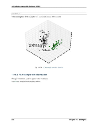
![scikit-learn user guide, Release 0.16.0
Python source code: plot_pca_iris.py
print(__doc__)
# Code source: Gaël Varoquaux
# License: BSD 3 clause
import numpy as np
import matplotlib.pyplot as plt
from mpl_toolkits.mplot3d import Axes3D
from sklearn import decomposition
from sklearn import datasets
np.random.seed(5)
centers = [[1, 1], [-1, -1], [1, -1]]
iris = datasets.load_iris()
X = iris.data
y = iris.target
fig = plt.figure(1, figsize=(4, 3))
plt.clf()
ax = Axes3D(fig, rect=[0, 0, .95, 1], elev=48, azim=134)
plt.cla()
pca = decomposition.PCA(n_components=3)
pca.fit(X)
X = pca.transform(X)
for name, label in [('Setosa', 0), ('Versicolour', 1), ('Virginica', 2)]:
ax.text3D(X[y == label, 0].mean(),
X[y == label, 1].mean() + 1.5,
X[y == label, 2].mean(), name,
horizontalalignment='center',
bbox=dict(alpha=.5, edgecolor='w', facecolor='w'))
11.10. Decomposition 551](https://image.slidesharecdn.com/scikit-learn0-150409112902-conversion-gate01/85/Scikit-learn-0-16-0-user-guide-561-320.jpg)
![scikit-learn user guide, Release 0.16.0
# Reorder the labels to have colors matching the cluster results
y = np.choose(y, [1, 2, 0]).astype(np.float)
ax.scatter(X[:, 0], X[:, 1], X[:, 2], c=y, cmap=plt.cm.spectral)
x_surf = [X[:, 0].min(), X[:, 0].max(),
X[:, 0].min(), X[:, 0].max()]
y_surf = [X[:, 0].max(), X[:, 0].max(),
X[:, 0].min(), X[:, 0].min()]
x_surf = np.array(x_surf)
y_surf = np.array(y_surf)
v0 = pca.transform(pca.components_[0])
v0 /= v0[-1]
v1 = pca.transform(pca.components_[1])
v1 /= v1[-1]
ax.w_xaxis.set_ticklabels([])
ax.w_yaxis.set_ticklabels([])
ax.w_zaxis.set_ticklabels([])
plt.show()
Total running time of the example: 0.08 seconds ( 0 minutes 0.08 seconds)
Fig. 11.72: Blind source separation using FastICA
11.10.4 Blind source separation using FastICA
An example of estimating sources from noisy data.
552 Chapter 11. Examples](https://image.slidesharecdn.com/scikit-learn0-150409112902-conversion-gate01/85/Scikit-learn-0-16-0-user-guide-562-320.jpg)
![scikit-learn user guide, Release 0.16.0
Independent component analysis (ICA) is used to estimate sources given noisy measurements. Imagine 3 instruments
playing simultaneously and 3 microphones recording the mixed signals. ICA is used to recover the sources ie. what
is played by each instrument. Importantly, PCA fails at recovering our instruments since the related signals reflect
non-Gaussian processes.
Python source code: plot_ica_blind_source_separation.py
print(__doc__)
import numpy as np
import matplotlib.pyplot as plt
from scipy import signal
from sklearn.decomposition import FastICA, PCA
###############################################################################
# Generate sample data
np.random.seed(0)
n_samples = 2000
time = np.linspace(0, 8, n_samples)
s1 = np.sin(2 * time) # Signal 1 : sinusoidal signal
s2 = np.sign(np.sin(3 * time)) # Signal 2 : square signal
s3 = signal.sawtooth(2 * np.pi * time) # Signal 3: saw tooth signal
S = np.c_[s1, s2, s3]
11.10. Decomposition 553](https://image.slidesharecdn.com/scikit-learn0-150409112902-conversion-gate01/85/Scikit-learn-0-16-0-user-guide-563-320.jpg)
![scikit-learn user guide, Release 0.16.0
S += 0.2 * np.random.normal(size=S.shape) # Add noise
S /= S.std(axis=0) # Standardize data
# Mix data
A = np.array([[1, 1, 1], [0.5, 2, 1.0], [1.5, 1.0, 2.0]]) # Mixing matrix
X = np.dot(S, A.T) # Generate observations
# Compute ICA
ica = FastICA(n_components=3)
S_ = ica.fit_transform(X) # Reconstruct signals
A_ = ica.mixing_ # Get estimated mixing matrix
# We can `prove` that the ICA model applies by reverting the unmixing.
assert np.allclose(X, np.dot(S_, A_.T) + ica.mean_)
# For comparison, compute PCA
pca = PCA(n_components=3)
H = pca.fit_transform(X) # Reconstruct signals based on orthogonal components
###############################################################################
# Plot results
plt.figure()
models = [X, S, S_, H]
names = ['Observations (mixed signal)',
'True Sources',
'ICA recovered signals',
'PCA recovered signals']
colors = ['red', 'steelblue', 'orange']
for ii, (model, name) in enumerate(zip(models, names), 1):
plt.subplot(4, 1, ii)
plt.title(name)
for sig, color in zip(model.T, colors):
plt.plot(sig, color=color)
plt.subplots_adjust(0.09, 0.04, 0.94, 0.94, 0.26, 0.46)
plt.show()
Total running time of the example: 0.17 seconds ( 0 minutes 0.17 seconds)
11.10.5 Kernel PCA
This example shows that Kernel PCA is able to find a projection of the data that makes data linearly separable.
554 Chapter 11. Examples](https://image.slidesharecdn.com/scikit-learn0-150409112902-conversion-gate01/85/Scikit-learn-0-16-0-user-guide-564-320.jpg)
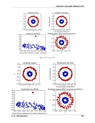
![scikit-learn user guide, Release 0.16.0
Python source code: plot_kernel_pca.py
print(__doc__)
# Authors: Mathieu Blondel
# Andreas Mueller
# License: BSD 3 clause
import numpy as np
import matplotlib.pyplot as plt
from sklearn.decomposition import PCA, KernelPCA
from sklearn.datasets import make_circles
np.random.seed(0)
X, y = make_circles(n_samples=400, factor=.3, noise=.05)
kpca = KernelPCA(kernel="rbf", fit_inverse_transform=True, gamma=10)
X_kpca = kpca.fit_transform(X)
X_back = kpca.inverse_transform(X_kpca)
pca = PCA()
X_pca = pca.fit_transform(X)
# Plot results
plt.figure()
plt.subplot(2, 2, 1, aspect='equal')
plt.title("Original space")
reds = y == 0
blues = y == 1
plt.plot(X[reds, 0], X[reds, 1], "ro")
plt.plot(X[blues, 0], X[blues, 1], "bo")
plt.xlabel("$x_1$")
plt.ylabel("$x_2$")
X1, X2 = np.meshgrid(np.linspace(-1.5, 1.5, 50), np.linspace(-1.5, 1.5, 50))
X_grid = np.array([np.ravel(X1), np.ravel(X2)]).T
# projection on the first principal component (in the phi space)
Z_grid = kpca.transform(X_grid)[:, 0].reshape(X1.shape)
plt.contour(X1, X2, Z_grid, colors='grey', linewidths=1, origin='lower')
plt.subplot(2, 2, 2, aspect='equal')
plt.plot(X_pca[reds, 0], X_pca[reds, 1], "ro")
plt.plot(X_pca[blues, 0], X_pca[blues, 1], "bo")
plt.title("Projection by PCA")
plt.xlabel("1st principal component")
plt.ylabel("2nd component")
plt.subplot(2, 2, 3, aspect='equal')
plt.plot(X_kpca[reds, 0], X_kpca[reds, 1], "ro")
plt.plot(X_kpca[blues, 0], X_kpca[blues, 1], "bo")
plt.title("Projection by KPCA")
plt.xlabel("1st principal component in space induced by $phi$")
plt.ylabel("2nd component")
plt.subplot(2, 2, 4, aspect='equal')
plt.plot(X_back[reds, 0], X_back[reds, 1], "ro")
556 Chapter 11. Examples](https://image.slidesharecdn.com/scikit-learn0-150409112902-conversion-gate01/85/Scikit-learn-0-16-0-user-guide-566-320.jpg)
![scikit-learn user guide, Release 0.16.0
plt.plot(X_back[blues, 0], X_back[blues, 1], "bo")
plt.title("Original space after inverse transform")
plt.xlabel("$x_1$")
plt.ylabel("$x_2$")
plt.subplots_adjust(0.02, 0.10, 0.98, 0.94, 0.04, 0.35)
plt.show()
Total running time of the example: 2.45 seconds ( 0 minutes 2.45 seconds)
Fig. 11.74: FastICA on 2D point clouds
11.10.6 FastICA on 2D point clouds
This example illustrates visually in the feature space a comparison by results using two different component analysis
techniques.
Independent component analysis (ICA) vs Principal component analysis (PCA).
Representing ICA in the feature space gives the view of ‘geometric ICA’: ICA is an algorithm that finds directions in
the feature space corresponding to projections with high non-Gaussianity. These directions need not be orthogonal in
the original feature space, but they are orthogonal in the whitened feature space, in which all directions correspond to
the same variance.
PCA, on the other hand, finds orthogonal directions in the raw feature space that correspond to directions accounting
for maximum variance.
Here we simulate independent sources using a highly non-Gaussian process, 2 student T with a low number of degrees
of freedom (top left figure). We mix them to create observations (top right figure). In this raw observation space,
11.10. Decomposition 557](https://image.slidesharecdn.com/scikit-learn0-150409112902-conversion-gate01/85/Scikit-learn-0-16-0-user-guide-567-320.jpg)
![scikit-learn user guide, Release 0.16.0
directions identified by PCA are represented by orange vectors. We represent the signal in the PCA space, after
whitening by the variance corresponding to the PCA vectors (lower left). Running ICA corresponds to finding a
rotation in this space to identify the directions of largest non-Gaussianity (lower right).
Python source code: plot_ica_vs_pca.py
print(__doc__)
# Authors: Alexandre Gramfort, Gael Varoquaux
# License: BSD 3 clause
import numpy as np
import matplotlib.pyplot as plt
from sklearn.decomposition import PCA, FastICA
###############################################################################
# Generate sample data
rng = np.random.RandomState(42)
S = rng.standard_t(1.5, size=(20000, 2))
S[:, 0] *= 2.
# Mix data
A = np.array([[1, 1], [0, 2]]) # Mixing matrix
X = np.dot(S, A.T) # Generate observations
558 Chapter 11. Examples](https://image.slidesharecdn.com/scikit-learn0-150409112902-conversion-gate01/85/Scikit-learn-0-16-0-user-guide-568-320.jpg)
![scikit-learn user guide, Release 0.16.0
pca = PCA()
S_pca_ = pca.fit(X).transform(X)
ica = FastICA(random_state=rng)
S_ica_ = ica.fit(X).transform(X) # Estimate the sources
S_ica_ /= S_ica_.std(axis=0)
###############################################################################
# Plot results
def plot_samples(S, axis_list=None):
plt.scatter(S[:, 0], S[:, 1], s=2, marker='o', linewidths=0, zorder=10,
color='steelblue', alpha=0.5)
if axis_list is not None:
colors = ['orange', 'red']
for color, axis in zip(colors, axis_list):
axis /= axis.std()
x_axis, y_axis = axis
# Trick to get legend to work
plt.plot(0.1 * x_axis, 0.1 * y_axis, linewidth=2, color=color)
plt.quiver(0, 0, x_axis, y_axis, zorder=11, width=0.01, scale=6,
color=color)
plt.hlines(0, -3, 3)
plt.vlines(0, -3, 3)
plt.xlim(-3, 3)
plt.ylim(-3, 3)
plt.xlabel('x')
plt.ylabel('y')
plt.figure()
plt.subplot(2, 2, 1)
plot_samples(S / S.std())
plt.title('True Independent Sources')
axis_list = [pca.components_.T, ica.mixing_]
plt.subplot(2, 2, 2)
plot_samples(X / np.std(X), axis_list=axis_list)
legend = plt.legend(['PCA', 'ICA'], loc='upper right')
legend.set_zorder(100)
plt.title('Observations')
plt.subplot(2, 2, 3)
plot_samples(S_pca_ / np.std(S_pca_, axis=0))
plt.title('PCA recovered signals')
plt.subplot(2, 2, 4)
plot_samples(S_ica_ / np.std(S_ica_))
plt.title('ICA recovered signals')
plt.subplots_adjust(0.09, 0.04, 0.94, 0.94, 0.26, 0.36)
plt.show()
Total running time of the example: 0.21 seconds ( 0 minutes 0.21 seconds)
11.10. Decomposition 559](https://image.slidesharecdn.com/scikit-learn0-150409112902-conversion-gate01/85/Scikit-learn-0-16-0-user-guide-569-320.jpg)
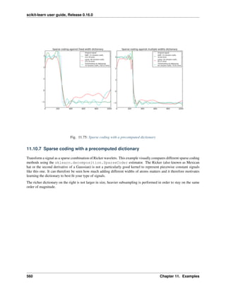
![scikit-learn user guide, Release 0.16.0
Python source code: plot_sparse_coding.py
print(__doc__)
import numpy as np
import matplotlib.pylab as pl
from sklearn.decomposition import SparseCoder
def ricker_function(resolution, center, width):
"""Discrete sub-sampled Ricker (Mexican hat) wavelet"""
x = np.linspace(0, resolution - 1, resolution)
x = ((2 / ((np.sqrt(3 * width) * np.pi ** 1 / 4)))
* (1 - ((x - center) ** 2 / width ** 2))
* np.exp((-(x - center) ** 2) / (2 * width ** 2)))
return x
def ricker_matrix(width, resolution, n_components):
"""Dictionary of Ricker (Mexican hat) wavelets"""
centers = np.linspace(0, resolution - 1, n_components)
D = np.empty((n_components, resolution))
for i, center in enumerate(centers):
D[i] = ricker_function(resolution, center, width)
D /= np.sqrt(np.sum(D ** 2, axis=1))[:, np.newaxis]
return D
resolution = 1024
subsampling = 3 # subsampling factor
width = 100
n_components = resolution / subsampling
# Compute a wavelet dictionary
D_fixed = ricker_matrix(width=width, resolution=resolution,
n_components=n_components)
D_multi = np.r_[tuple(ricker_matrix(width=w, resolution=resolution,
11.10. Decomposition 561](https://image.slidesharecdn.com/scikit-learn0-150409112902-conversion-gate01/85/Scikit-learn-0-16-0-user-guide-571-320.jpg)
![scikit-learn user guide, Release 0.16.0
n_components=np.floor(n_components / 5))
for w in (10, 50, 100, 500, 1000))]
# Generate a signal
y = np.linspace(0, resolution - 1, resolution)
first_quarter = y < resolution / 4
y[first_quarter] = 3.
y[np.logical_not(first_quarter)] = -1.
# List the different sparse coding methods in the following format:
# (title, transform_algorithm, transform_alpha, transform_n_nozero_coefs)
estimators = [('OMP', 'omp', None, 15), ('Lasso', 'lasso_cd', 2, None), ]
pl.figure(figsize=(13, 6))
for subplot, (D, title) in enumerate(zip((D_fixed, D_multi),
('fixed width', 'multiple widths'))):
pl.subplot(1, 2, subplot + 1)
pl.title('Sparse coding against %s dictionary' % title)
pl.plot(y, ls='dotted', label='Original signal')
# Do a wavelet approximation
for title, algo, alpha, n_nonzero in estimators:
coder = SparseCoder(dictionary=D, transform_n_nonzero_coefs=n_nonzero,
transform_alpha=alpha, transform_algorithm=algo)
x = coder.transform(y)
density = len(np.flatnonzero(x))
x = np.ravel(np.dot(x, D))
squared_error = np.sum((y - x) ** 2)
pl.plot(x, label='%s: %s nonzero coefs,n%.2f error'
% (title, density, squared_error))
# Soft thresholding debiasing
coder = SparseCoder(dictionary=D, transform_algorithm='threshold',
transform_alpha=20)
x = coder.transform(y)
_, idx = np.where(x != 0)
x[0, idx], _, _, _ = np.linalg.lstsq(D[idx, :].T, y)
x = np.ravel(np.dot(x, D))
squared_error = np.sum((y - x) ** 2)
pl.plot(x,
label='Thresholding w/ debiasing:n%d nonzero coefs, %.2f error' %
(len(idx), squared_error))
pl.axis('tight')
pl.legend()
pl.subplots_adjust(.04, .07, .97, .90, .09, .2)
pl.show()
Total running time of the example: 0.77 seconds ( 0 minutes 0.77 seconds)
11.10.8 Principal components analysis (PCA)
These figures aid in illustrating how a point cloud can be very flat in one direction–which is where PCA comes in to
choose a direction that is not flat.
562 Chapter 11. Examples](https://image.slidesharecdn.com/scikit-learn0-150409112902-conversion-gate01/85/Scikit-learn-0-16-0-user-guide-572-320.jpg)
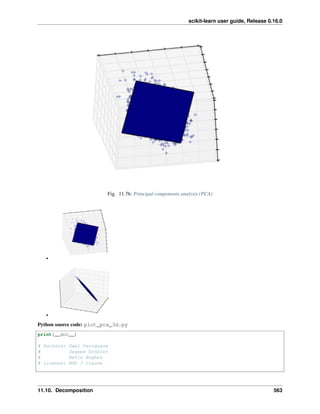
![scikit-learn user guide, Release 0.16.0
from sklearn.decomposition import PCA
from mpl_toolkits.mplot3d import Axes3D
import numpy as np
import matplotlib.pyplot as plt
from scipy import stats
###############################################################################
# Create the data
e = np.exp(1)
np.random.seed(4)
def pdf(x):
return 0.5 * (stats.norm(scale=0.25 / e).pdf(x)
+ stats.norm(scale=4 / e).pdf(x))
y = np.random.normal(scale=0.5, size=(30000))
x = np.random.normal(scale=0.5, size=(30000))
z = np.random.normal(scale=0.1, size=len(x))
density = pdf(x) * pdf(y)
pdf_z = pdf(5 * z)
density *= pdf_z
a = x + y
b = 2 * y
c = a - b + z
norm = np.sqrt(a.var() + b.var())
a /= norm
b /= norm
###############################################################################
# Plot the figures
def plot_figs(fig_num, elev, azim):
fig = plt.figure(fig_num, figsize=(4, 3))
plt.clf()
ax = Axes3D(fig, rect=[0, 0, .95, 1], elev=elev, azim=azim)
ax.scatter(a[::10], b[::10], c[::10], c=density[::10], marker='+', alpha=.4)
Y = np.c_[a, b, c]
# Using SciPy's SVD, this would be:
# _, pca_score, V = scipy.linalg.svd(Y, full_matrices=False)
pca = PCA(n_components=3)
pca.fit(Y)
pca_score = pca.explained_variance_ratio_
V = pca.components_
x_pca_axis, y_pca_axis, z_pca_axis = V.T * pca_score / pca_score.min()
x_pca_axis, y_pca_axis, z_pca_axis = 3 * V.T
564 Chapter 11. Examples](https://image.slidesharecdn.com/scikit-learn0-150409112902-conversion-gate01/85/Scikit-learn-0-16-0-user-guide-574-320.jpg)
![scikit-learn user guide, Release 0.16.0
x_pca_plane = np.r_[x_pca_axis[:2], - x_pca_axis[1::-1]]
y_pca_plane = np.r_[y_pca_axis[:2], - y_pca_axis[1::-1]]
z_pca_plane = np.r_[z_pca_axis[:2], - z_pca_axis[1::-1]]
x_pca_plane.shape = (2, 2)
y_pca_plane.shape = (2, 2)
z_pca_plane.shape = (2, 2)
ax.plot_surface(x_pca_plane, y_pca_plane, z_pca_plane)
ax.w_xaxis.set_ticklabels([])
ax.w_yaxis.set_ticklabels([])
ax.w_zaxis.set_ticklabels([])
elev = -40
azim = -80
plot_figs(1, elev, azim)
elev = 30
azim = 20
plot_figs(2, elev, azim)
plt.show()
Total running time of the example: 0.13 seconds ( 0 minutes 0.13 seconds)
Fig. 11.77: Model selection with Probabilistic (PCA) and Factor Analysis (FA)
11.10. Decomposition 565](https://image.slidesharecdn.com/scikit-learn0-150409112902-conversion-gate01/85/Scikit-learn-0-16-0-user-guide-575-320.jpg)

![scikit-learn user guide, Release 0.16.0
# Authors: Alexandre Gramfort
# Denis A. Engemann
# License: BSD 3 clause
import numpy as np
import matplotlib.pyplot as plt
from scipy import linalg
from sklearn.decomposition import PCA, FactorAnalysis
from sklearn.covariance import ShrunkCovariance, LedoitWolf
from sklearn.cross_validation import cross_val_score
from sklearn.grid_search import GridSearchCV
###############################################################################
# Create the data
n_samples, n_features, rank = 1000, 50, 10
sigma = 1.
rng = np.random.RandomState(42)
U, _, _ = linalg.svd(rng.randn(n_features, n_features))
X = np.dot(rng.randn(n_samples, rank), U[:, :rank].T)
# Adding homoscedastic noise
X_homo = X + sigma * rng.randn(n_samples, n_features)
# Adding heteroscedastic noise
sigmas = sigma * rng.rand(n_features) + sigma / 2.
X_hetero = X + rng.randn(n_samples, n_features) * sigmas
###############################################################################
# Fit the models
n_components = np.arange(0, n_features, 5) # options for n_components
def compute_scores(X):
pca = PCA()
fa = FactorAnalysis()
pca_scores, fa_scores = [], []
for n in n_components:
pca.n_components = n
fa.n_components = n
pca_scores.append(np.mean(cross_val_score(pca, X)))
fa_scores.append(np.mean(cross_val_score(fa, X)))
return pca_scores, fa_scores
def shrunk_cov_score(X):
shrinkages = np.logspace(-2, 0, 30)
cv = GridSearchCV(ShrunkCovariance(), {'shrinkage': shrinkages})
return np.mean(cross_val_score(cv.fit(X).best_estimator_, X))
def lw_score(X):
return np.mean(cross_val_score(LedoitWolf(), X))
11.10. Decomposition 567](https://image.slidesharecdn.com/scikit-learn0-150409112902-conversion-gate01/85/Scikit-learn-0-16-0-user-guide-577-320.jpg)
![scikit-learn user guide, Release 0.16.0
for X, title in [(X_homo, 'Homoscedastic Noise'),
(X_hetero, 'Heteroscedastic Noise')]:
pca_scores, fa_scores = compute_scores(X)
n_components_pca = n_components[np.argmax(pca_scores)]
n_components_fa = n_components[np.argmax(fa_scores)]
pca = PCA(n_components='mle')
pca.fit(X)
n_components_pca_mle = pca.n_components_
print("best n_components by PCA CV = %d" % n_components_pca)
print("best n_components by FactorAnalysis CV = %d" % n_components_fa)
print("best n_components by PCA MLE = %d" % n_components_pca_mle)
plt.figure()
plt.plot(n_components, pca_scores, 'b', label='PCA scores')
plt.plot(n_components, fa_scores, 'r', label='FA scores')
plt.axvline(rank, color='g', label='TRUTH: %d' % rank, linestyle='-')
plt.axvline(n_components_pca, color='b',
label='PCA CV: %d' % n_components_pca, linestyle='--')
plt.axvline(n_components_fa, color='r',
label='FactorAnalysis CV: %d' % n_components_fa, linestyle='--')
plt.axvline(n_components_pca_mle, color='k',
label='PCA MLE: %d' % n_components_pca_mle, linestyle='--')
# compare with other covariance estimators
plt.axhline(shrunk_cov_score(X), color='violet',
label='Shrunk Covariance MLE', linestyle='-.')
plt.axhline(lw_score(X), color='orange',
label='LedoitWolf MLE' % n_components_pca_mle, linestyle='-.')
plt.xlabel('nb of components')
plt.ylabel('CV scores')
plt.legend(loc='lower right')
plt.title(title)
plt.show()
Total running time of the example: 44.29 seconds ( 0 minutes 44.29 seconds)
11.10.10 Faces dataset decompositions
This example applies to The Olivetti faces dataset different unsupervised matrix decomposition (dimension reduction)
methods from the module sklearn.decomposition (see the documentation chapter Decomposing signals in
components (matrix factorization problems)) .
568 Chapter 11. Examples](https://image.slidesharecdn.com/scikit-learn0-150409112902-conversion-gate01/85/Scikit-learn-0-16-0-user-guide-578-320.jpg)


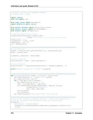
![scikit-learn user guide, Release 0.16.0
('Non-negative components - NMF',
decomposition.NMF(n_components=n_components, init='nndsvda', beta=5.0,
tol=5e-3, sparseness='components'),
False),
('Independent components - FastICA',
decomposition.FastICA(n_components=n_components, whiten=True),
True),
('Sparse comp. - MiniBatchSparsePCA',
decomposition.MiniBatchSparsePCA(n_components=n_components, alpha=0.8,
n_iter=100, batch_size=3,
random_state=rng),
True),
('MiniBatchDictionaryLearning',
decomposition.MiniBatchDictionaryLearning(n_components=15, alpha=0.1,
n_iter=50, batch_size=3,
random_state=rng),
True),
('Cluster centers - MiniBatchKMeans',
MiniBatchKMeans(n_clusters=n_components, tol=1e-3, batch_size=20,
max_iter=50, random_state=rng),
True),
('Factor Analysis components - FA',
decomposition.FactorAnalysis(n_components=n_components, max_iter=2),
True),
]
###############################################################################
# Plot a sample of the input data
plot_gallery("First centered Olivetti faces", faces_centered[:n_components])
###############################################################################
# Do the estimation and plot it
for name, estimator, center in estimators:
print("Extracting the top %d %s..." % (n_components, name))
t0 = time()
data = faces
if center:
data = faces_centered
estimator.fit(data)
train_time = (time() - t0)
print("done in %0.3fs" % train_time)
if hasattr(estimator, 'cluster_centers_'):
components_ = estimator.cluster_centers_
else:
components_ = estimator.components_
if hasattr(estimator, 'noise_variance_'):
plot_gallery("Pixelwise variance",
estimator.noise_variance_.reshape(1, -1), n_col=1,
n_row=1)
plot_gallery('%s - Train time %.1fs' % (name, train_time),
11.10. Decomposition 573](https://image.slidesharecdn.com/scikit-learn0-150409112902-conversion-gate01/85/Scikit-learn-0-16-0-user-guide-583-320.jpg)
![scikit-learn user guide, Release 0.16.0
components_[:n_components])
plt.show()
Total running time of the example: 14.30 seconds ( 0 minutes 14.30 seconds)
Fig. 11.79: Image denoising using dictionary learning
11.10.11 Image denoising using dictionary learning
An example comparing the effect of reconstructing noisy fragments of the Lena image using firstly online Dictionary
Learning and various transform methods.
The dictionary is fitted on the distorted left half of the image, and subsequently used to reconstruct the right half. Note
that even better performance could be achieved by fitting to an undistorted (i.e. noiseless) image, but here we start
from the assumption that it is not available.
A common practice for evaluating the results of image denoising is by looking at the difference between the recon-
struction and the original image. If the reconstruction is perfect this will look like Gaussian noise.
It can be seen from the plots that the results of Orthogonal Matching Pursuit (OMP) with two non-zero coefficients is
a bit less biased than when keeping only one (the edges look less prominent). It is in addition closer from the ground
truth in Frobenius norm.
The result of Least Angle Regression is much more strongly biased: the difference is reminiscent of the local intensity
value of the original image.
Thresholding is clearly not useful for denoising, but it is here to show that it can produce a suggestive output with
very high speed, and thus be useful for other tasks such as object classification, where performance is not necessarily
related to visualisation.
574 Chapter 11. Examples](https://image.slidesharecdn.com/scikit-learn0-150409112902-conversion-gate01/85/Scikit-learn-0-16-0-user-guide-584-320.jpg)

![scikit-learn user guide, Release 0.16.0
•
Script output:
Distorting image...
Extracting reference patches...
done in 0.02s.
Learning the dictionary...
done in 6.00s.
Extracting noisy patches...
done in 0.01s.
Orthogonal Matching Pursuit
1 atom...
done in 5.40s.
Orthogonal Matching Pursuit
2 atoms...
done in 8.64s.
Least-angle regression
5 atoms...
done in 27.42s.
Thresholding
alpha=0.1...
done in 1.75s.
Python source code: plot_image_denoising.py
print(__doc__)
from time import time
import matplotlib.pyplot as plt
import numpy as np
from scipy.misc import lena
from sklearn.decomposition import MiniBatchDictionaryLearning
from sklearn.feature_extraction.image import extract_patches_2d
from sklearn.feature_extraction.image import reconstruct_from_patches_2d
###############################################################################
# Load Lena image and extract patches
lena = lena() / 256.0
# downsample for higher speed
lena = lena[::2, ::2] + lena[1::2, ::2] + lena[::2, 1::2] + lena[1::2, 1::2]
lena /= 4.0
height, width = lena.shape
# Distort the right half of the image
576 Chapter 11. Examples](https://image.slidesharecdn.com/scikit-learn0-150409112902-conversion-gate01/85/Scikit-learn-0-16-0-user-guide-586-320.jpg)
![scikit-learn user guide, Release 0.16.0
print('Distorting image...')
distorted = lena.copy()
distorted[:, height // 2:] += 0.075 * np.random.randn(width, height // 2)
# Extract all reference patches from the left half of the image
print('Extracting reference patches...')
t0 = time()
patch_size = (7, 7)
data = extract_patches_2d(distorted[:, :height // 2], patch_size)
data = data.reshape(data.shape[0], -1)
data -= np.mean(data, axis=0)
data /= np.std(data, axis=0)
print('done in %.2fs.' % (time() - t0))
###############################################################################
# Learn the dictionary from reference patches
print('Learning the dictionary...')
t0 = time()
dico = MiniBatchDictionaryLearning(n_components=100, alpha=1, n_iter=500)
V = dico.fit(data).components_
dt = time() - t0
print('done in %.2fs.' % dt)
plt.figure(figsize=(4.2, 4))
for i, comp in enumerate(V[:100]):
plt.subplot(10, 10, i + 1)
plt.imshow(comp.reshape(patch_size), cmap=plt.cm.gray_r,
interpolation='nearest')
plt.xticks(())
plt.yticks(())
plt.suptitle('Dictionary learned from Lena patchesn' +
'Train time %.1fs on %d patches' % (dt, len(data)),
fontsize=16)
plt.subplots_adjust(0.08, 0.02, 0.92, 0.85, 0.08, 0.23)
###############################################################################
# Display the distorted image
def show_with_diff(image, reference, title):
"""Helper function to display denoising"""
plt.figure(figsize=(5, 3.3))
plt.subplot(1, 2, 1)
plt.title('Image')
plt.imshow(image, vmin=0, vmax=1, cmap=plt.cm.gray, interpolation='nearest')
plt.xticks(())
plt.yticks(())
plt.subplot(1, 2, 2)
difference = image - reference
plt.title('Difference (norm: %.2f)' % np.sqrt(np.sum(difference ** 2)))
plt.imshow(difference, vmin=-0.5, vmax=0.5, cmap=plt.cm.PuOr,
interpolation='nearest')
plt.xticks(())
plt.yticks(())
plt.suptitle(title, size=16)
plt.subplots_adjust(0.02, 0.02, 0.98, 0.79, 0.02, 0.2)
11.10. Decomposition 577](https://image.slidesharecdn.com/scikit-learn0-150409112902-conversion-gate01/85/Scikit-learn-0-16-0-user-guide-587-320.jpg)
![scikit-learn user guide, Release 0.16.0
show_with_diff(distorted, lena, 'Distorted image')
###############################################################################
# Extract noisy patches and reconstruct them using the dictionary
print('Extracting noisy patches... ')
t0 = time()
data = extract_patches_2d(distorted[:, height // 2:], patch_size)
data = data.reshape(data.shape[0], -1)
intercept = np.mean(data, axis=0)
data -= intercept
print('done in %.2fs.' % (time() - t0))
transform_algorithms = [
('Orthogonal Matching Pursuitn1 atom', 'omp',
{'transform_n_nonzero_coefs': 1}),
('Orthogonal Matching Pursuitn2 atoms', 'omp',
{'transform_n_nonzero_coefs': 2}),
('Least-angle regressionn5 atoms', 'lars',
{'transform_n_nonzero_coefs': 5}),
('Thresholdingn alpha=0.1', 'threshold', {'transform_alpha': .1})]
reconstructions = {}
for title, transform_algorithm, kwargs in transform_algorithms:
print(title + '...')
reconstructions[title] = lena.copy()
t0 = time()
dico.set_params(transform_algorithm=transform_algorithm, **kwargs)
code = dico.transform(data)
patches = np.dot(code, V)
if transform_algorithm == 'threshold':
patches -= patches.min()
patches /= patches.max()
patches += intercept
patches = patches.reshape(len(data), *patch_size)
if transform_algorithm == 'threshold':
patches -= patches.min()
patches /= patches.max()
reconstructions[title][:, height // 2:] = reconstruct_from_patches_2d(
patches, (width, height // 2))
dt = time() - t0
print('done in %.2fs.' % dt)
show_with_diff(reconstructions[title], lena,
title + ' (time: %.1fs)' % dt)
plt.show()
Total running time of the example: 56.48 seconds ( 0 minutes 56.48 seconds)
11.11 Ensemble methods
Examples concerning the sklearn.ensemble module.
578 Chapter 11. Examples](https://image.slidesharecdn.com/scikit-learn0-150409112902-conversion-gate01/85/Scikit-learn-0-16-0-user-guide-588-320.jpg)


![scikit-learn user guide, Release 0.16.0
data = fetch_olivetti_faces()
X = data.images.reshape((len(data.images), -1))
y = data.target
mask = y < 5 # Limit to 5 classes
X = X[mask]
y = y[mask]
# Build a forest and compute the pixel importances
print("Fitting ExtraTreesClassifier on faces data with %d cores..." % n_jobs)
t0 = time()
forest = ExtraTreesClassifier(n_estimators=1000,
max_features=128,
n_jobs=n_jobs,
random_state=0)
forest.fit(X, y)
print("done in %0.3fs" % (time() - t0))
importances = forest.feature_importances_
importances = importances.reshape(data.images[0].shape)
# Plot pixel importances
plt.matshow(importances, cmap=plt.cm.hot)
plt.title("Pixel importances with forests of trees")
plt.show()
Total running time of the example: 0.88 seconds ( 0 minutes 0.88 seconds)
Fig. 11.81: Decision Tree Regression with AdaBoost
11.11. Ensemble methods 581](https://image.slidesharecdn.com/scikit-learn0-150409112902-conversion-gate01/85/Scikit-learn-0-16-0-user-guide-591-320.jpg)
![scikit-learn user guide, Release 0.16.0
11.11.2 Decision Tree Regression with AdaBoost
A decision tree is boosted using the AdaBoost.R2 [1] algorithm on a 1D sinusoidal dataset with a small amount of
Gaussian noise. 299 boosts (300 decision trees) is compared with a single decision tree regressor. As the number of
boosts is increased the regressor can fit more detail.
Python source code: plot_adaboost_regression.py
print(__doc__)
# Author: Noel Dawe <noel.dawe@gmail.com>
#
# License: BSD 3 clause
# importing necessary libraries
import numpy as np
import matplotlib.pyplot as plt
from sklearn.tree import DecisionTreeRegressor
from sklearn.ensemble import AdaBoostRegressor
# Create the dataset
rng = np.random.RandomState(1)
X = np.linspace(0, 6, 100)[:, np.newaxis]
y = np.sin(X).ravel() + np.sin(6 * X).ravel() + rng.normal(0, 0.1, X.shape[0])
# Fit regression model
582 Chapter 11. Examples](https://image.slidesharecdn.com/scikit-learn0-150409112902-conversion-gate01/85/Scikit-learn-0-16-0-user-guide-592-320.jpg)


![scikit-learn user guide, Release 0.16.0
from sklearn.datasets import make_classification
from sklearn.ensemble import ExtraTreesClassifier
# Build a classification task using 3 informative features
X, y = make_classification(n_samples=1000,
n_features=10,
n_informative=3,
n_redundant=0,
n_repeated=0,
n_classes=2,
random_state=0,
shuffle=False)
# Build a forest and compute the feature importances
forest = ExtraTreesClassifier(n_estimators=250,
random_state=0)
forest.fit(X, y)
importances = forest.feature_importances_
std = np.std([tree.feature_importances_ for tree in forest.estimators_],
axis=0)
indices = np.argsort(importances)[::-1]
# Print the feature ranking
print("Feature ranking:")
for f in range(10):
print("%d. feature %d (%f)" % (f + 1, indices[f], importances[indices[f]]))
# Plot the feature importances of the forest
plt.figure()
plt.title("Feature importances")
plt.bar(range(10), importances[indices],
color="r", yerr=std[indices], align="center")
plt.xticks(range(10), indices)
plt.xlim([-1, 10])
plt.show()
Total running time of the example: 0.34 seconds ( 0 minutes 0.34 seconds)
11.11.4 Gradient Boosting regularization
Illustration of the effect of different regularization strategies for Gradient Boosting. The example is taken from Hastie
et al 2009.
The loss function used is binomial deviance. Regularization via shrinkage (learning_rate < 1.0) improves
performance considerably. In combination with shrinkage, stochastic gradient boosting (subsample < 1.0) can
produce more accurate models by reducing the variance via bagging. Subsampling without shrinkage usually does
poorly. Another strategy to reduce the variance is by subsampling the features analogous to the random splits in
Random Forests (via the max_features parameter).
11.11. Ensemble methods 585](https://image.slidesharecdn.com/scikit-learn0-150409112902-conversion-gate01/85/Scikit-learn-0-16-0-user-guide-595-320.jpg)

![scikit-learn user guide, Release 0.16.0
Python source code: plot_gradient_boosting_regularization.py
print(__doc__)
# Author: Peter Prettenhofer <peter.prettenhofer@gmail.com>
#
# License: BSD 3 clause
import numpy as np
import matplotlib.pyplot as plt
from sklearn import ensemble
from sklearn import datasets
X, y = datasets.make_hastie_10_2(n_samples=12000, random_state=1)
X = X.astype(np.float32)
# map labels from {-1, 1} to {0, 1}
labels, y = np.unique(y, return_inverse=True)
X_train, X_test = X[:2000], X[2000:]
y_train, y_test = y[:2000], y[2000:]
original_params = {'n_estimators': 1000, 'max_leaf_nodes': 4, 'max_depth': None, 'random_state': 2,
'min_samples_split': 5}
plt.figure()
for label, color, setting in [('No shrinkage', 'orange',
{'learning_rate': 1.0, 'subsample': 1.0}),
('learning_rate=0.1', 'turquoise',
{'learning_rate': 0.1, 'subsample': 1.0}),
('subsample=0.5', 'blue',
{'learning_rate': 1.0, 'subsample': 0.5}),
('learning_rate=0.1, subsample=0.5', 'gray',
{'learning_rate': 0.1, 'subsample': 0.5}),
('learning_rate=0.1, max_features=2', 'magenta',
{'learning_rate': 0.1, 'max_features': 2})]:
params = dict(original_params)
params.update(setting)
clf = ensemble.GradientBoostingClassifier(**params)
clf.fit(X_train, y_train)
# compute test set deviance
test_deviance = np.zeros((params['n_estimators'],), dtype=np.float64)
for i, y_pred in enumerate(clf.staged_decision_function(X_test)):
# clf.loss_ assumes that y_test[i] in {0, 1}
test_deviance[i] = clf.loss_(y_test, y_pred)
plt.plot((np.arange(test_deviance.shape[0]) + 1)[::5], test_deviance[::5],
'-', color=color, label=label)
plt.legend(loc='upper left')
plt.xlabel('Boosting Iterations')
plt.ylabel('Test Set Deviance')
11.11. Ensemble methods 587](https://image.slidesharecdn.com/scikit-learn0-150409112902-conversion-gate01/85/Scikit-learn-0-16-0-user-guide-597-320.jpg)
![scikit-learn user guide, Release 0.16.0
plt.show()
Total running time of the example: 23.68 seconds ( 0 minutes 23.68 seconds)
Fig. 11.84: Partial Dependence Plots
11.11.5 Partial Dependence Plots
Partial dependence plots show the dependence between the target function 2
and a set of ‘target’ features, marginalizing
over the values of all other features (the complement features). Due to the limits of human perception the size of the
target feature set must be small (usually, one or two) thus the target features are usually chosen among the most
important features (see feature_importances_).
This example shows how to obtain partial dependence plots from a GradientBoostingRegressor trained on
the California housing dataset. The example is taken from [HTF2009].
The plot shows four one-way and one two-way partial dependence plots. The target variables for the one-way PDP
are: median income (MedInc), avg. occupants per household (AvgOccup), median house age (HouseAge), and avg.
rooms per household (AveRooms).
We can clearly see that the median house price shows a linear relationship with the median income (top left) and that
the house price drops when the avg. occupants per household increases (top middle). The top right plot shows that the
house age in a district does not have a strong influence on the (median) house price; so does the average rooms per
household. The tick marks on the x-axis represent the deciles of the feature values in the training data.
Partial dependence plots with two target features enable us to visualize interactions among them. The two-way partial
dependence plot shows the dependence of median house price on joint values of house age and avg. occupants per
household. We can clearly see an interaction between the two features: For an avg. occupancy greater than two, the
2 For classification you can think of it as the regression score before the link function.
588 Chapter 11. Examples](https://image.slidesharecdn.com/scikit-learn0-150409112902-conversion-gate01/85/Scikit-learn-0-16-0-user-guide-598-320.jpg)

![scikit-learn user guide, Release 0.16.0
# split 80/20 train-test
X_train, X_test, y_train, y_test = train_test_split(cal_housing.data,
cal_housing.target,
test_size=0.2,
random_state=1)
names = cal_housing.feature_names
print('_' * 80)
print("Training GBRT...")
clf = GradientBoostingRegressor(n_estimators=100, max_depth=4,
learning_rate=0.1, loss='huber',
random_state=1)
clf.fit(X_train, y_train)
print("done.")
print('_' * 80)
print('Convenience plot with ``partial_dependence_plots``')
print
features = [0, 5, 1, 2, (5, 1)]
fig, axs = plot_partial_dependence(clf, X_train, features, feature_names=names,
n_jobs=3, grid_resolution=50)
fig.suptitle('Partial dependence of house value on nonlocation featuresn'
'for the California housing dataset')
plt.subplots_adjust(top=0.9) # tight_layout causes overlap with suptitle
print('_' * 80)
print('Custom 3d plot via ``partial_dependence``')
print
fig = plt.figure()
target_feature = (1, 5)
pdp, (x_axis, y_axis) = partial_dependence(clf, target_feature,
X=X_train, grid_resolution=50)
XX, YY = np.meshgrid(x_axis, y_axis)
Z = pdp.T.reshape(XX.shape).T
ax = Axes3D(fig)
surf = ax.plot_surface(XX, YY, Z, rstride=1, cstride=1, cmap=plt.cm.BuPu)
ax.set_xlabel(names[target_feature[0]])
ax.set_ylabel(names[target_feature[1]])
ax.set_zlabel('Partial dependence')
# pretty init view
ax.view_init(elev=22, azim=122)
plt.colorbar(surf)
plt.suptitle('Partial dependence of house value on median age and '
'average occupancy')
plt.subplots_adjust(top=0.9)
plt.show()
Total running time of the example: 4.03 seconds ( 0 minutes 4.03 seconds)
11.11.6 Gradient Boosting regression
Demonstrate Gradient Boosting on the Boston housing dataset.
This example fits a Gradient Boosting model with least squares loss and 500 regression trees of depth 4.
590 Chapter 11. Examples](https://image.slidesharecdn.com/scikit-learn0-150409112902-conversion-gate01/85/Scikit-learn-0-16-0-user-guide-600-320.jpg)

![scikit-learn user guide, Release 0.16.0
print(__doc__)
# Author: Peter Prettenhofer <peter.prettenhofer@gmail.com>
#
# License: BSD 3 clause
import numpy as np
import matplotlib.pyplot as plt
from sklearn import ensemble
from sklearn import datasets
from sklearn.utils import shuffle
from sklearn.metrics import mean_squared_error
###############################################################################
# Load data
boston = datasets.load_boston()
X, y = shuffle(boston.data, boston.target, random_state=13)
X = X.astype(np.float32)
offset = int(X.shape[0] * 0.9)
X_train, y_train = X[:offset], y[:offset]
X_test, y_test = X[offset:], y[offset:]
###############################################################################
# Fit regression model
params = {'n_estimators': 500, 'max_depth': 4, 'min_samples_split': 1,
'learning_rate': 0.01, 'loss': 'ls'}
clf = ensemble.GradientBoostingRegressor(**params)
clf.fit(X_train, y_train)
mse = mean_squared_error(y_test, clf.predict(X_test))
print("MSE: %.4f" % mse)
###############################################################################
# Plot training deviance
# compute test set deviance
test_score = np.zeros((params['n_estimators'],), dtype=np.float64)
for i, y_pred in enumerate(clf.staged_decision_function(X_test)):
test_score[i] = clf.loss_(y_test, y_pred)
plt.figure(figsize=(12, 6))
plt.subplot(1, 2, 1)
plt.title('Deviance')
plt.plot(np.arange(params['n_estimators']) + 1, clf.train_score_, 'b-',
label='Training Set Deviance')
plt.plot(np.arange(params['n_estimators']) + 1, test_score, 'r-',
label='Test Set Deviance')
plt.legend(loc='upper right')
plt.xlabel('Boosting Iterations')
plt.ylabel('Deviance')
###############################################################################
# Plot feature importance
feature_importance = clf.feature_importances_
# make importances relative to max importance
feature_importance = 100.0 * (feature_importance / feature_importance.max())
592 Chapter 11. Examples](https://image.slidesharecdn.com/scikit-learn0-150409112902-conversion-gate01/85/Scikit-learn-0-16-0-user-guide-602-320.jpg)
![scikit-learn user guide, Release 0.16.0
sorted_idx = np.argsort(feature_importance)
pos = np.arange(sorted_idx.shape[0]) + .5
plt.subplot(1, 2, 2)
plt.barh(pos, feature_importance[sorted_idx], align='center')
plt.yticks(pos, boston.feature_names[sorted_idx])
plt.xlabel('Relative Importance')
plt.title('Variable Importance')
plt.show()
Total running time of the example: 1.13 seconds ( 0 minutes 1.13 seconds)
Fig. 11.86: Prediction Intervals for Gradient Boosting Regression
11.11.7 Prediction Intervals for Gradient Boosting Regression
This example shows how quantile regression can be used to create prediction intervals.
11.11. Ensemble methods 593](https://image.slidesharecdn.com/scikit-learn0-150409112902-conversion-gate01/85/Scikit-learn-0-16-0-user-guide-603-320.jpg)
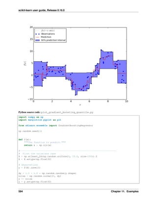
![scikit-learn user guide, Release 0.16.0
# Mesh the input space for evaluations of the real function, the prediction and
# its MSE
xx = np.atleast_2d(np.linspace(0, 10, 1000)).T
xx = xx.astype(np.float32)
alpha = 0.95
clf = GradientBoostingRegressor(loss='quantile', alpha=alpha,
n_estimators=250, max_depth=3,
learning_rate=.1, min_samples_leaf=9,
min_samples_split=9)
clf.fit(X, y)
# Make the prediction on the meshed x-axis
y_upper = clf.predict(xx)
clf.set_params(alpha=1.0 - alpha)
clf.fit(X, y)
# Make the prediction on the meshed x-axis
y_lower = clf.predict(xx)
clf.set_params(loss='ls')
clf.fit(X, y)
# Make the prediction on the meshed x-axis
y_pred = clf.predict(xx)
# Plot the function, the prediction and the 90% confidence interval based on
# the MSE
fig = plt.figure()
plt.plot(xx, f(xx), 'g:', label=u'$f(x) = x,sin(x)$')
plt.plot(X, y, 'b.', markersize=10, label=u'Observations')
plt.plot(xx, y_pred, 'r-', label=u'Prediction')
plt.plot(xx, y_upper, 'k-')
plt.plot(xx, y_lower, 'k-')
plt.fill(np.concatenate([xx, xx[::-1]]),
np.concatenate([y_upper, y_lower[::-1]]),
alpha=.5, fc='b', ec='None', label='90% prediction interval')
plt.xlabel('$x$')
plt.ylabel('$f(x)$')
plt.ylim(-10, 20)
plt.legend(loc='upper left')
plt.show()
Total running time of the example: 0.39 seconds ( 0 minutes 0.39 seconds)
11.11.8 Hashing feature transformation using Totally Random Trees
RandomTreesEmbedding provides a way to map data to a very high-dimensional, sparse representation, which might
be beneficial for classification. The mapping is completely unsupervised and very efficient.
This example visualizes the partitions given by several trees and shows how the transformation can also be used for
non-linear dimensionality reduction or non-linear classification.
Points that are neighboring often share the same leaf of a tree and therefore share large parts of their hashed repre-
11.11. Ensemble methods 595](https://image.slidesharecdn.com/scikit-learn0-150409112902-conversion-gate01/85/Scikit-learn-0-16-0-user-guide-605-320.jpg)


![scikit-learn user guide, Release 0.16.0
# Learn a Naive Bayes classifier on the transformed data
nb = BernoulliNB()
nb.fit(X_transformed, y)
# Learn an ExtraTreesClassifier for comparison
trees = ExtraTreesClassifier(max_depth=3, n_estimators=10, random_state=0)
trees.fit(X, y)
# scatter plot of original and reduced data
fig = plt.figure(figsize=(9, 8))
ax = plt.subplot(221)
ax.scatter(X[:, 0], X[:, 1], c=y, s=50)
ax.set_title("Original Data (2d)")
ax.set_xticks(())
ax.set_yticks(())
ax = plt.subplot(222)
ax.scatter(X_reduced[:, 0], X_reduced[:, 1], c=y, s=50)
ax.set_title("PCA reduction (2d) of transformed data (%dd)" %
X_transformed.shape[1])
ax.set_xticks(())
ax.set_yticks(())
# Plot the decision in original space. For that, we will assign a color to each
# point in the mesh [x_min, m_max] x [y_min, y_max].
h = .01
x_min, x_max = X[:, 0].min() - .5, X[:, 0].max() + .5
y_min, y_max = X[:, 1].min() - .5, X[:, 1].max() + .5
xx, yy = np.meshgrid(np.arange(x_min, x_max, h), np.arange(y_min, y_max, h))
# transform grid using RandomTreesEmbedding
transformed_grid = hasher.transform(np.c_[xx.ravel(), yy.ravel()])
y_grid_pred = nb.predict_proba(transformed_grid)[:, 1]
ax = plt.subplot(223)
ax.set_title("Naive Bayes on Transformed data")
ax.pcolormesh(xx, yy, y_grid_pred.reshape(xx.shape))
ax.scatter(X[:, 0], X[:, 1], c=y, s=50)
ax.set_ylim(-1.4, 1.4)
ax.set_xlim(-1.4, 1.4)
ax.set_xticks(())
ax.set_yticks(())
# transform grid using ExtraTreesClassifier
y_grid_pred = trees.predict_proba(np.c_[xx.ravel(), yy.ravel()])[:, 1]
ax = plt.subplot(224)
ax.set_title("ExtraTrees predictions")
ax.pcolormesh(xx, yy, y_grid_pred.reshape(xx.shape))
ax.scatter(X[:, 0], X[:, 1], c=y, s=50)
ax.set_ylim(-1.4, 1.4)
ax.set_xlim(-1.4, 1.4)
ax.set_xticks(())
ax.set_yticks(())
598 Chapter 11. Examples](https://image.slidesharecdn.com/scikit-learn0-150409112902-conversion-gate01/85/Scikit-learn-0-16-0-user-guide-608-320.jpg)


![scikit-learn user guide, Release 0.16.0
plt.figure(figsize=(10, 5))
# Plot the decision boundaries
plt.subplot(121)
x_min, x_max = X[:, 0].min() - 1, X[:, 0].max() + 1
y_min, y_max = X[:, 1].min() - 1, X[:, 1].max() + 1
xx, yy = np.meshgrid(np.arange(x_min, x_max, plot_step),
np.arange(y_min, y_max, plot_step))
Z = bdt.predict(np.c_[xx.ravel(), yy.ravel()])
Z = Z.reshape(xx.shape)
cs = plt.contourf(xx, yy, Z, cmap=plt.cm.Paired)
plt.axis("tight")
# Plot the training points
for i, n, c in zip(range(2), class_names, plot_colors):
idx = np.where(y == i)
plt.scatter(X[idx, 0], X[idx, 1],
c=c, cmap=plt.cm.Paired,
label="Class %s" % n)
plt.xlim(x_min, x_max)
plt.ylim(y_min, y_max)
plt.legend(loc='upper right')
plt.xlabel('x')
plt.ylabel('y')
plt.title('Decision Boundary')
# Plot the two-class decision scores
twoclass_output = bdt.decision_function(X)
plot_range = (twoclass_output.min(), twoclass_output.max())
plt.subplot(122)
for i, n, c in zip(range(2), class_names, plot_colors):
plt.hist(twoclass_output[y == i],
bins=10,
range=plot_range,
facecolor=c,
label='Class %s' % n,
alpha=.5)
x1, x2, y1, y2 = plt.axis()
plt.axis((x1, x2, y1, y2 * 1.2))
plt.legend(loc='upper right')
plt.ylabel('Samples')
plt.xlabel('Score')
plt.title('Decision Scores')
plt.tight_layout()
plt.subplots_adjust(wspace=0.35)
plt.show()
Total running time of the example: 4.94 seconds ( 0 minutes 4.94 seconds)
11.11.10 Discrete versus Real AdaBoost
This example is based on Figure 10.2 from Hastie et al 2009 [1] and illustrates the difference in performance between
the discrete SAMME [2] boosting algorithm and real SAMME.R boosting algorithm. Both algorithms are evaluated
on a binary classification task where the target Y is a non-linear function of 10 input features.
11.11. Ensemble methods 601](https://image.slidesharecdn.com/scikit-learn0-150409112902-conversion-gate01/85/Scikit-learn-0-16-0-user-guide-611-320.jpg)

![scikit-learn user guide, Release 0.16.0
Python source code: plot_adaboost_hastie_10_2.py
print(__doc__)
# Author: Peter Prettenhofer <peter.prettenhofer@gmail.com>,
# Noel Dawe <noel.dawe@gmail.com>
#
# License: BSD 3 clause
import numpy as np
import matplotlib.pyplot as plt
from sklearn import datasets
from sklearn.tree import DecisionTreeClassifier
from sklearn.metrics import zero_one_loss
from sklearn.ensemble import AdaBoostClassifier
n_estimators = 400
# A learning rate of 1. may not be optimal for both SAMME and SAMME.R
learning_rate = 1.
X, y = datasets.make_hastie_10_2(n_samples=12000, random_state=1)
X_test, y_test = X[2000:], y[2000:]
X_train, y_train = X[:2000], y[:2000]
11.11. Ensemble methods 603](https://image.slidesharecdn.com/scikit-learn0-150409112902-conversion-gate01/85/Scikit-learn-0-16-0-user-guide-613-320.jpg)
![scikit-learn user guide, Release 0.16.0
dt_stump = DecisionTreeClassifier(max_depth=1, min_samples_leaf=1)
dt_stump.fit(X_train, y_train)
dt_stump_err = 1.0 - dt_stump.score(X_test, y_test)
dt = DecisionTreeClassifier(max_depth=9, min_samples_leaf=1)
dt.fit(X_train, y_train)
dt_err = 1.0 - dt.score(X_test, y_test)
ada_discrete = AdaBoostClassifier(
base_estimator=dt_stump,
learning_rate=learning_rate,
n_estimators=n_estimators,
algorithm="SAMME")
ada_discrete.fit(X_train, y_train)
ada_real = AdaBoostClassifier(
base_estimator=dt_stump,
learning_rate=learning_rate,
n_estimators=n_estimators,
algorithm="SAMME.R")
ada_real.fit(X_train, y_train)
fig = plt.figure()
ax = fig.add_subplot(111)
ax.plot([1, n_estimators], [dt_stump_err] * 2, 'k-',
label='Decision Stump Error')
ax.plot([1, n_estimators], [dt_err] * 2, 'k--',
label='Decision Tree Error')
ada_discrete_err = np.zeros((n_estimators,))
for i, y_pred in enumerate(ada_discrete.staged_predict(X_test)):
ada_discrete_err[i] = zero_one_loss(y_pred, y_test)
ada_discrete_err_train = np.zeros((n_estimators,))
for i, y_pred in enumerate(ada_discrete.staged_predict(X_train)):
ada_discrete_err_train[i] = zero_one_loss(y_pred, y_train)
ada_real_err = np.zeros((n_estimators,))
for i, y_pred in enumerate(ada_real.staged_predict(X_test)):
ada_real_err[i] = zero_one_loss(y_pred, y_test)
ada_real_err_train = np.zeros((n_estimators,))
for i, y_pred in enumerate(ada_real.staged_predict(X_train)):
ada_real_err_train[i] = zero_one_loss(y_pred, y_train)
ax.plot(np.arange(n_estimators) + 1, ada_discrete_err,
label='Discrete AdaBoost Test Error',
color='red')
ax.plot(np.arange(n_estimators) + 1, ada_discrete_err_train,
label='Discrete AdaBoost Train Error',
color='blue')
ax.plot(np.arange(n_estimators) + 1, ada_real_err,
label='Real AdaBoost Test Error',
color='orange')
ax.plot(np.arange(n_estimators) + 1, ada_real_err_train,
label='Real AdaBoost Train Error',
color='green')
604 Chapter 11. Examples](https://image.slidesharecdn.com/scikit-learn0-150409112902-conversion-gate01/85/Scikit-learn-0-16-0-user-guide-614-320.jpg)


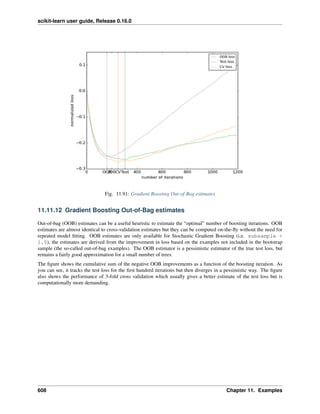


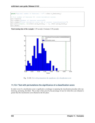


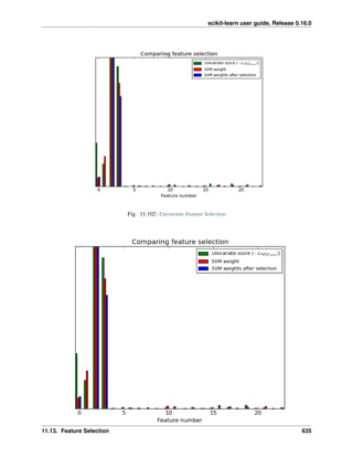
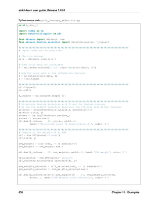
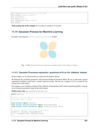

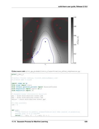
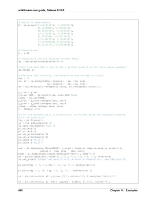


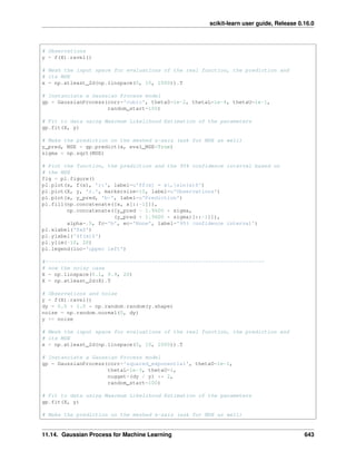


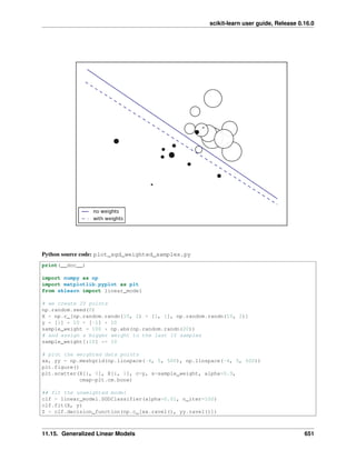


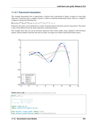


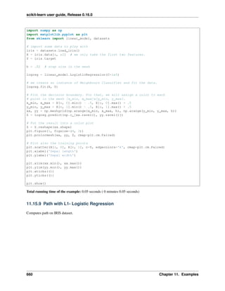

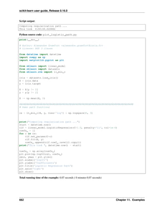


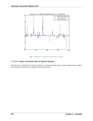
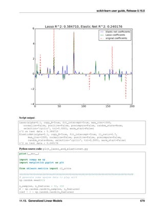


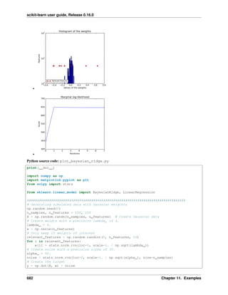


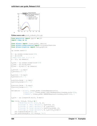


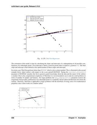


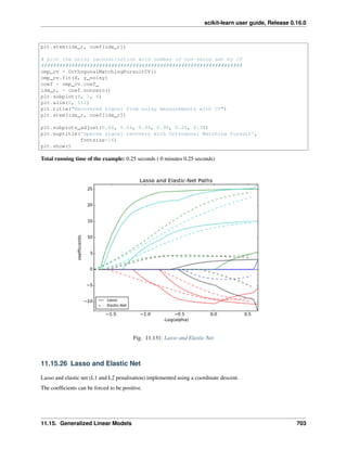


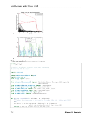


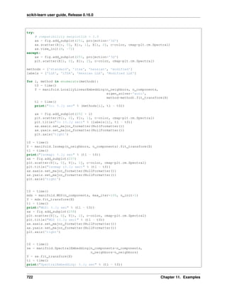

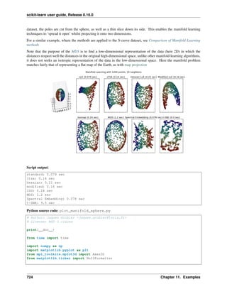


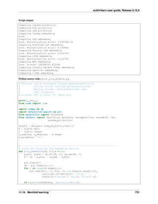

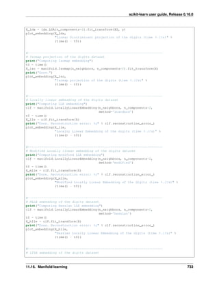


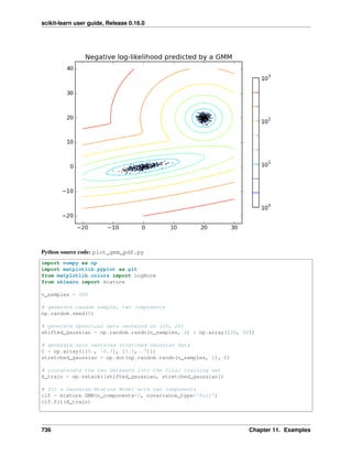


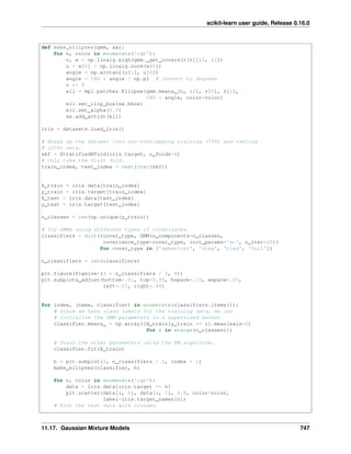


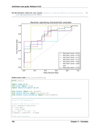


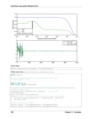


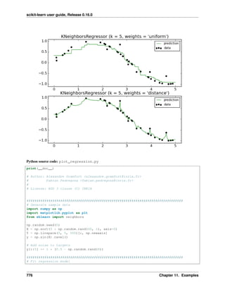
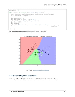


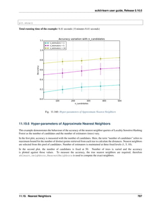
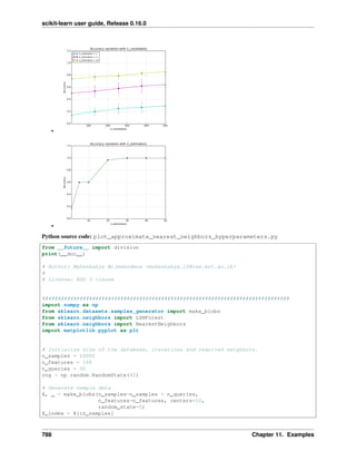


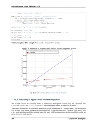


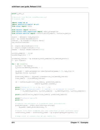


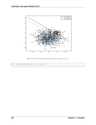


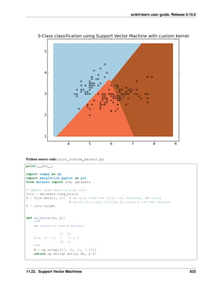


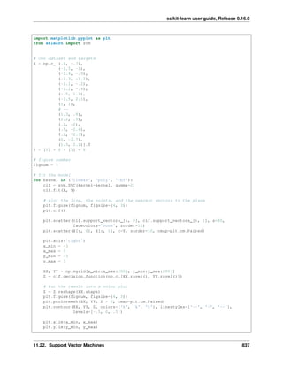


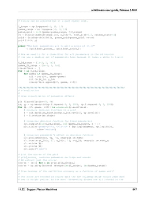


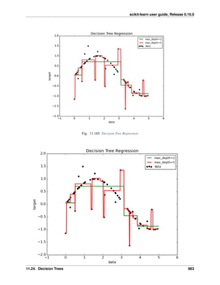

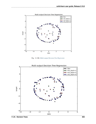


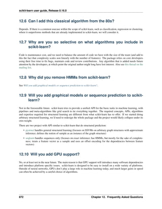


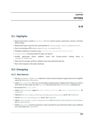


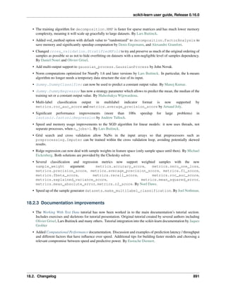


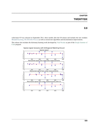


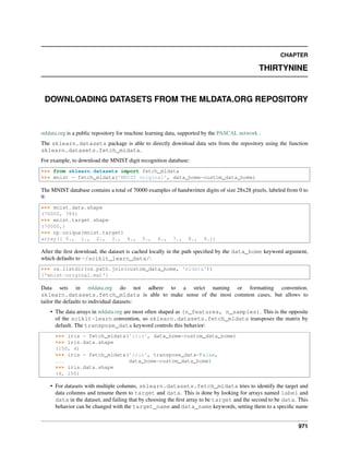


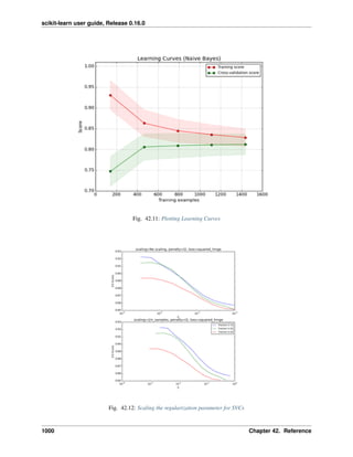
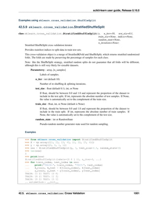


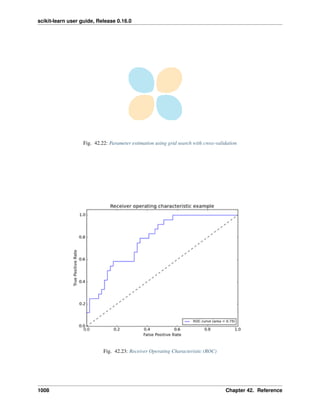


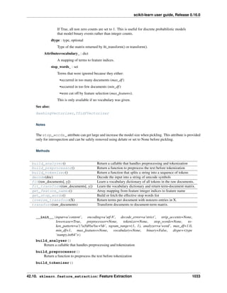


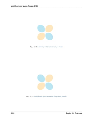


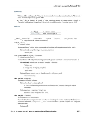


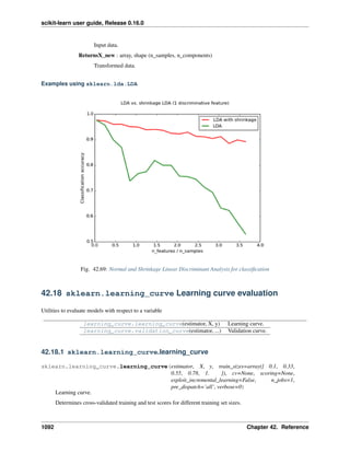


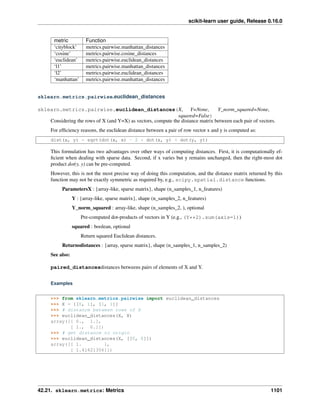


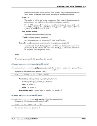


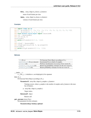


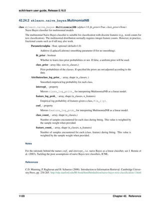


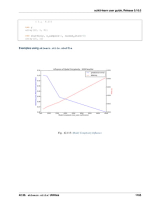


This document is a user guide for scikit-learn, an open-source machine learning library for Python. It provides tutorials and documentation on machine learning techniques including supervised learning algorithms like linear models, support vector machines, decision trees, and unsupervised learning algorithms like clustering and dimensionality reduction. The guide covers loading and preprocessing data, model fitting and prediction, evaluating performance, and parameter tuning. It also includes examples demonstrating how to apply the library's algorithms to real-world problems.