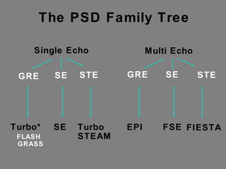
6. Single Echo GRE SE STE Turbo* FLASH GRASS SE Turbo STEAM Subsecond Easy to run Flexible Popular Poor SNR Popular... Conventional Keyholed... Seconds More difficult Very flexible Popular
7. Multi Echo GRE SE STE EPI Spiral FSE FIESTA Subsecond 10Hz Difficult/expensive Very flexible Good SNR Intense interest Seconds to minutes Easy, SAR Very flexible Good SNR Very popular Fast but sensitive To field inhomogeneities
8. K-space covers Frequency and Phase Frequency Phase Sequences: GRE SE FSE Turbo GRE EPI Spiral Sampling VB 1/2NEX 1/2 Echo Key Hole
9. k-Space and MRI Physics Phase Frequency hi lo + - hi FT lo "sample spin echo" slice phase frequency 90 rf 180 rf Frequency Phase
10. The MR Sequence Determines How k-space is Sampled... 90 180 view 1 192 The "spin-echo" 128 64 256 view 1 view 256 Frequency Slice selection
11. High-Speed MRI Families GRE SE Turbo single echo multi echo EPI multi echo FSE ~ 1 sec ez to do ~ 32 msec strong gradients needed... 10 sec - 6 min. SE tissue contrasts
12. High-Speed GRE Family GRE SPGR spoiled Refocused GRE GRASS MPGR Appears T1-wt Useful for GM-WM 3D GRE uses SPGR for anatomy - MP-RAGE Appears T2-wt. Useful for MRA, flow, CSF, MS
13. GRE vs. EPI Slice Frequency Phase Partial flip Partial flip echo echo echo echo echo
14. GRE vs. EPI One view every TR... All views in one TR! Note where the "center echo" - this is the key to TEf - the effectve TE!
17. Spiral Scanning Segmented sampling Done with less than 1 gauss/cm Non-linear ADC sampling Incredible applications (fast, flow sensitvie) slice x-gradient y-gradient
18. LAD Spiral-scan 512X512 surface coil 15 cm FOV acquired over 4 breath holds 80 spirals Zero TE FID image Meyer et al. Stanford
19. Transverse Magnetization builds up for short TR values in Gradient-echo MRI!! For long T2* protons, the in-plane dephasing is not completed prior to the next TR... (and the next view with a differing phase!!!) The result is a view-to view variation of signal phase and image intensity.... ARTIFACTS SOLUTION: 1. "rewind" view to view phase change... 2. "spoil" view to view phase change REFOCUS OR SPOIL REWIND OR REFOCUS - GRASS, MPGR SPOIL - SPGR
21. SI slice selection gradients FID RF "sinc" pulse 4 msec sampling time dephase TR 10-100 gradient-echo still dephasing for 4XT2* Transverse magnetization builds up from view to view.
22. SI slice selection gradients FID RF "sinc" pulse 4 msec sampling time dephase "rewinds" phase from view to view REWIND OR REFOCUS
23. SI slice selection gradients FID RF "sinc" pulse - VARY PHASE OF EACH PULSE 4 msec sampling time dephase "rewinds" phase from view to view SPOILED GRASS KILLER
24. Contrast in GRE TR 200 TE 15 MPGR 5 o 45 o 75 o For long TR: Increase in flip adds T1-wting.....
25. Contrast in GRE TR 200, Flip 30, MPGR For long TE in GRE: Increase in TE adds T2-wting..... and MS artifacts 6 ms 30 ms
27. Basic Rules of GRE Tissue Contrast SPGR - Gives (nearly always) T1-weighted contrast For best T1-weighting: TR short 20- 100 TE short as possible < 10 Flips from 30-45
28. In General... Small flip angles enhances proton density (PD). Increasing flip leads to more T1-weighting. Increasing TE leads to more T2, T2*-weighting. Increasing TR, decreasing flip leads to more PD. Mechanisms in Action Steady-state transverse phase loss - T2, T2* Longitudinal recovery - T1 FRE, magnetic susceptibility - FRE, MS
29. GRE - Mutants "Fast" GRE - Done with short TR = "Turbo" "Center out" - Do the center views first to minimize T1 saturation... "DE" - Driven equilibrium - does a 90 - 180 - GRE to create a "T2- like" tissue contrast... "IR" - Inversion recovery to give T1 weighting... F/W phase - adjusts TE to make fat/water in phase useful to help minimize lipids
30. SE vs. FSE Slice Frequency Phase 90 180 echo 90 180 180 180 180 180
31. sample frequency increment phase change FSE k-space sampling is simply view by view
32. FSE Advantages Short scan times!! TR 2000, 512X512, 2 NEX = 34 minutes Scan time = TR x #views x NEX TR 2000, 512X512, 2 NEX , ET 16 = 2 minutes!!
33. The "effective TE" in FSE is determined by where the "center views" (LEAST AMOUNT OF PHASE ENCODING!) are collected... Effective TE in FSE FSE 90 180 echo Phase encoding Where is the center view? What is the eff. TE??
34. Effect of TE TR 5000 TE 85 TE 119 TE 136 TE 102 FSE allows long TR's... helps TE effect by reducing T1 contributions!!
35. FSE Issues Total TR 8 echoes give 6 slices... 16 echoes give 3 slices...
36. SI Time (msec) 17 34 51 68 85 102 136 153 msec Long ET trains increase T2-weighting... For longer ET trains, the later echoes contribute greatly... This is ET 16!!
37. Effect of TE TR 5000 TE 85 TE 119 TE 136 TE 102 FSE allows long TR's... helps TE effect by reducing T1 contributions!!
38. Effect of ET TR 4000 TE 102 ET 4 ET 16 ET 8 Increasing ET increases T2 effects... By increasing the contribution from the later echoes...
39. FSE has unique applicatons in the body.. TR 2000 TE 85 ET 16 128X256 1 NEX BREATH HELD!
40. FSE has bright fat.. Virtues of FATSAT... TR 6000 TE 119
41. Chem Sat (FatSat) 1. Wide range of clinical advantages: Anatomy free of lipids (or water!) Better SNR (dynamic range is increased, as is amplifier gain) Definition of hyperintensity as fat/fluid. Reduction of fat-enhanced respiratory artifacts!! NO chemical shift misregistration VB now possible 2. Clinical roles: Better depiction of joint fluids Improved Gd enhancement
42. How does FATSAT work? The chemical shift is due to the different proton environments of water and lipids... frequency Water Lipids 220 Hz + + This chemcial shift is responsible for the "Chemical shift artifact"
43. How does FATSAT work? Apply a long (16 msec) rf pulse exactly at the lipid resonance but miss the water resonance... frequency Water Lipids + + This chemcial shift is responsible for the "Chemical shift artifact" Bandwidth of rf pulse = 100Hz
44. How does FATSAT work? Apply a long (16 msec) rf pulse exactly at the lipid resonance but miss the water resonance... The "sinc" pulse profile has a square bandwidth.. Time Frequency RF pulse length related to RF bandwidth center frequency bandwidth
45. How does FATSAT work? Now that lipids are excited... Crush phase coherence with a strong GRADIENT! SAT RF "Crush" 90 RF 180 RF gradient Excites only lipids 220 Hz from water Spoils phase coherence Begin next view with 90 - 180 - echo...
47. Steady-state Free Precession - 1 With improved gradient capabilities in recent years that permit the use of ultrashort TRs, SSFP has gained wide popularity for various applications in cardiac imaging,35,82,95 flow imaging,96 T1/T2 quantification,97,98 whole body imaging,99 etc. SSFP is a unique sequence in that it belongs to both the spin-echo and gradient-echo families. In an SSFP sequence, a gradient-echo is acquired similar to a FLASH or FISP sequence. However, the gradient structure is symmetrically balanced in the slice, phase-encoding, and read directions (Fig. 5-32) and no RF spoiling is implemented. Coherences are maintained in successive RF cycles so that the transverse magnetization from one TR contributes to the signal in the succeeding TRs. The RF echoes generated by the train of α pulses in the steady state are then superimposed on the gradient-echo (assuming a uniform main field). Signal is therefore highlighted from long-T2* and long-T2 components. Since there is no magnetization spoiling, there are no saturation effects as in spoiled techniques, and high flip angles can be used in SSFP. The balanced and symmetric gradient structure also generates motion insensitivity because of first-order gradient moment nulling. While the TR remains shorter than T2 and there is no RF spoiling, the magnetization develops a coherent steady state, which is a combination of the longitudinal and transverse components. Starting from equilibrium magnetization, a finite time is necessary for the magnetization to reach steady state, during which RF excitations are continuously applied. In steady state, the SSFP signal is T2/T1 weighted, which is a unique form of contrast and is seeing increasing applications for in vivo imaging. The SSFP signal is a complicated function of parameters such as TR, T1, T2, flip angle, and off-resonance angle β ( β = γ×Δ B0 × TR). Despite its many advantages, such as high SNR compared to spoiled gradient-echo sequences and high imaging efficiency, signal sensitivity to off-resonance is one of the major limitations of SSFP. page 166 Improved gradient capabilities -> ultrashort TRs SSFP for cardiac imaging, flow imaging T1/T2 quantification, whole body imaging SSFP is unique - both spin-echo and gradient-echo In SSFP A gradient-echo is acquired like FLASH or FISP But, gradients are symmetrically balanced in slice, phase-encoding, & read directions No RF spoiling is implemented.
48. Steady-state Free Precession - 2 Coherences are maintained in successive TRs. Transverse magnetization from one TR contributes to the next TRs. The RF echoes generated by the train of α pulses in the steady state are then added to the gradient-echo (assuming a uniform main field, this is the catch ). Signal is mostly from long-T2* and long-T2 tissues. No spoiling, so no saturation effects as in spoiled techniques, and high flip angles can be used in SSFP. Balanced gradients also mean motion insensitivity.
49. Steady-state Free Precession - 3 As long as TR is shorter than T2 without RF spoiling, we have a coherent steady state. That is a combination of the longitudinal and transverse components. It takes time to reach SS. In steady state, the SSFP signal is T2/T1 weighted. SSFP signal is a complicated function of parameters such as TR, T1, T2, flip angle, and off-resonance angle β ( β = γ×Δ B0 × TR). Advantages: unique contrast, high SNR compared to spoiled GRE & high imaging efficiency, but sensitivity to off-resonance is a major limitation.
51. Off-resonance Artifacts in SSFP Off-resonance artifacts are usually bands in SSFP. Main sources of off-resonance artifact B0 inhomogeneity. Static B0 field varies within an object. Artifacts can be minimized by careful shimming, high BW, shortest TR possible. Approach to Steady State 3 x T1 to reach steady state. Long T1 tissues may show artifact.
53. Reduced Scan time Data Acquisition Strategies Fractional Echo Partial Views SMASH Partial FOV SENSE Increased SNR Data Acquisition Strategies
54. SMASH - Simultaneous Acquisition of Spatial Harmonics Sodickson & Manning, MRM 38(4):591-603 (Oct. 1997) “ Linear combinations of simultaneously acquired signals from multiple surface coils with different spatial sensitivities to generate multiple data sets with distinct offsets in k-space.” Huh? Add signals from multiple coils using information about the coil’s spatial location
55. SMASH - Simultaneous Acquisition of Spatial Harmonics Sodickson & Manning, MRM 38(4):591-603 (Oct. 1997) S(k x ,k y )=∫ ∫ C(x,y)M(x,y) e -I(kx·x+ky ·y) dxdy Usually C(x,y) = 1 For SMASH, Construct coils with sinusoidal sensitivities, Like a gradient shift. 5 lines per readout with 4 spatial harmonics per readout
56. SMASH achieves a reduction in scantime, R, given by the number of simultaneously acquired spatial frequency harmonics. SMASH Procedure: 1. Determine sensitivity profile for each coil. 2. Determine the number of spatial harmonics that can be generated using the coil array. 3. Acquire data from coil array - these are aliased component coil images. 4. Determine weights for linear combinations of component coil signals. 5. Form composite k-space signals corresponding to the spatial harmonics. 6. Interleave the composite signals then Fourier transform. Weakness: Measurement & manipulation of sensitivity profiles.
57. SENSE: Sensitivity encoding Pruessmann, Weiger,Scheidegger,Boesigner. MRM 42(5):952-969 (Nov. 1999) “ Knowledge of coil sensitivity implies information about the detected MR signal which may be used in image generation.” Coil 2 Coil 1 Coil 4 Coil 3 SMASH requires the combination of coil sensitivity. SENSE is the generalization of SMASH for any geometry.
58. Aliasing: MRI data is collected in the frequency domain, so objects outside of the FOV fold back into the image. Analog Signal Over- sampled Under- sampled f1 f2 f1
59. Aliasing or Wrap-around in standard coil seen when FOV is smaller than the object being imaged. FOV x FOV y True positions Aliased positions
60. SENSE: Sensitivity encoding Pruessmann, Weiger,Scheidegger,Boesigner. MRM 42(5):952-969 (Nov. 1999) Coil 2 Coil 1 Coil 4 Coil 3 Reconstruction of an image from N receiver coils: Undersampled k-space from each receiver (aliasing). Undo signal superposition caused by fold-over (aliasing). Undo signal superposition by using weighting caused by varied coil sensitivities.
61. FOV=24cm, 384x256, 5mm slice, TR/TE=4400/97.4Ef ms EC=1/1, BW= 31.2 kHz, 2 NEX, VBW/TRF/Z512 WVU Twin-speed ACR Uniformity Slice: ASSET compatible FRFSE-XL/90 After ASSET cal. - ASSET turned on without SCIC with SCIC 8 Channel Brain Coil
62. FOV=24cm, 384x256, 5mm slice, TR/TE=4400/97.4Ef ms EC=1/1, BW= 31.2 kHz, 2 NEX, VBW/TRF/Z512 WVU Twin-speed ACR Uniformity Slice: ASSET compatible FRFSE-XL/90 After ASSET cal. - ASSET turned off without SCIC with SCIC 8 Channel Brain Coil
63. Problem is that while the SNR as measured by Center Signal / stdev of background is high, uniformity is poor. In a ROI of 500 mm 2 stdev = 50, or 25 w/SCIC. WVU Twin-speed ACR Uniformity Slice: ASSET compatible FRFSE-XL/90 with SCIC 8 Channel Brain Coil Quad Head Coil SNR w/SCIC = 195, wout/SCIC = 128 SNR= 95
64. WVU Twin-speed ACR Uniformity Slice: ASSET compatible FRFSE-XL/90 Coil Signal St.Dev. Head 622 11 8ch 677 50 8chSCIC 623 25 Measurements made in same location - as shown in image.