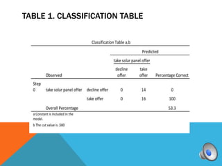
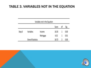
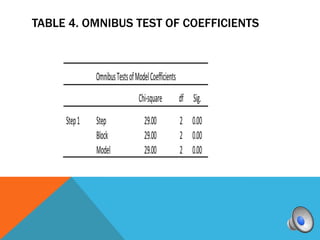
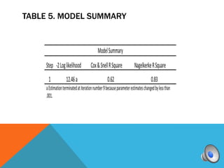
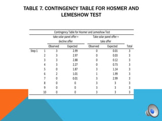
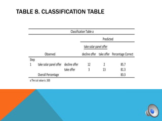
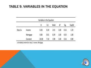
WHAT IS LOGISTIC REGRESSION?
 Logit for short, a specialized form of regression


 used when the dependent variable is dichotomous (has
  only two values 0 and 1) and categorical while the
  independent variable(s) could be any type


 There are many variables in the business world that are
  dichotomous, for example: male or female, to buy or not
  to buy, good credit risk or poor credit risks, to take offer
  or decline offer, student will succeed or fail, etc.
ASSUMPTIONS OF LOGISTIC REGRESSION
 Does not assume a linear relationship between DV and IV


 Dependent variable must be a dichotomy (2 categories)


 Independent variables need not be interval, nor normally
  distributed, nor linearly related, nor of equal variance within
  each group


 The categories of the DV must be mutually exclusive and
  exhaustive such that a case can only be in one group and
  every case must be a member of one of the groups
GOAL OF LOGISTIC REGRESSION
 logistic regression determines the impact of
  multiple independent variables presented
  simultaneously to predict membership of one or
  other of the two dependent variable categories
DESCRIPTION OF THE DATA
 The data used to conduct logistic regression is from a
  survey of 30 homeowners conducted by an electricity
  company about an offer of roof solar panels with a 50%
  subsidy from the state government as part of the state’s
  environmental policy.


 The variables are:
IVs:    household income measured in units of a thousand
dollars age of householder
       monthly mortgage
       size of family household
DV:    whether the householder would take or decline the
offer. Take the offer was coded as 1 and decline the offer
was coded     as 0.
WHAT IS THE RESEARCH QUESTION?

 to determine whether household income and monthly
  mortgage will predict taking or declining the solar panel
  offer


 Independent Variables: household income and monthly
  mortgage


 Dependent Variables: Take the offer or decline the offer
TWO HYPOTHESES TO BE TESTED
There are two hypotheses to test in relation to the
  overall fit of the model:


 H0: The model is a good fitting model


 H1: The model is not a good fitting model (i.e.
  the predictors have a significant effect)
HOW TO PERFORM LOGISTIC REGRESSION IN
                SPSS

1) Click Analyze
2) Select Regression
3) Select Binary Logistic
4) Select the dependent variable, the one which is a
   grouping variable (0 and 1) and place it into the
   Dependent Box, in this case, take or decline offer
5) Enter the predictors (IVs) that you want to test into the
   Covariates Box. In this case, Household Income and
   Monthly Mortgage
6) Leave Enter as the default method
CONTINUATION OF SPSS STEPS
7) If there is any categorical IV, click on Categorical button
and enter it. There is none in this case.


8) In the Options button, select Classification Plots, Hosmer-
Lemeshow goodness-of-fit, Casewise Listing of residuals.
Retain default entries for probability of stepwise,
classification cutoff, and maximum iterations


9) Continue, then, OK
TABLE 1. CLASSIFICATION TABLE
TABLE 2. VARIABLES IN THE EQUATION TABLE
TABLE 3. VARIABLES NOT IN THE EQUATION
TABLE 4. OMNIBUS TEST OF COEFFICIENTS
TABLE 5. MODEL SUMMARY
TABLE 6. HOSMER AND LEMESHOW TEST
TABLE 7. CONTINGENCY TABLE FOR HOSMER AND
               LEMESHOW TEST
TABLE 8. CLASSIFICATION TABLE
TABLE 9. VARIABLES IN THE EQUATION
 A logistic regression analysis was conducted to
  predict if householders will take up or decline
  the offer of a solar panel subsidy.

 Predictors --household income and mortgage
  payment

 A test of the full model against the constant
  model was statistically significant, indicating
  that the predictors as a set differentiated
  between acceptors and decliners of the offer
  (chi-square=29, p<.000 with df=2).
 Nagelkerke’s R2 of .83 indicated a moderately
  strong relationship between prediction and
  grouping. Prediction success overall was 83.3%
  (85.7% for decline and 81.3% for accept).


 The Wald criterion showed that both predictors
  were not significant predictors. ExpB value
  indicates that when household income is raised
  by one unit ($1,000), the odds ratio is 1.33 times
  as large and therefore householders are 1.33
  more times likely to take the offer.
 Since the predictors did not have a significant effect
  (p>.005), we fail to reject the null hypothesis that
  there is no difference between observed and model-
  predicted values, thus, the model is a good fitting
  model. Even if the two predictors did not show
  significant effect, they were able to distinguished
  between acceptors and decliners of the offer as the
  Chi-square table (Table 4) show.

 Perhaps, other predictors such as age and family
  size may have significant effect, or perhaps adding
  one more predictor, however, this paper only
  considered two independent variables.

Module5.slp

  • 2.
    WHAT IS LOGISTICREGRESSION?  Logit for short, a specialized form of regression  used when the dependent variable is dichotomous (has only two values 0 and 1) and categorical while the independent variable(s) could be any type  There are many variables in the business world that are dichotomous, for example: male or female, to buy or not to buy, good credit risk or poor credit risks, to take offer or decline offer, student will succeed or fail, etc.
  • 3.
    ASSUMPTIONS OF LOGISTICREGRESSION  Does not assume a linear relationship between DV and IV  Dependent variable must be a dichotomy (2 categories)  Independent variables need not be interval, nor normally distributed, nor linearly related, nor of equal variance within each group  The categories of the DV must be mutually exclusive and exhaustive such that a case can only be in one group and every case must be a member of one of the groups
  • 4.
    GOAL OF LOGISTICREGRESSION  logistic regression determines the impact of multiple independent variables presented simultaneously to predict membership of one or other of the two dependent variable categories
  • 6.
    DESCRIPTION OF THEDATA  The data used to conduct logistic regression is from a survey of 30 homeowners conducted by an electricity company about an offer of roof solar panels with a 50% subsidy from the state government as part of the state’s environmental policy.  The variables are: IVs: household income measured in units of a thousand dollars age of householder monthly mortgage size of family household DV: whether the householder would take or decline the offer. Take the offer was coded as 1 and decline the offer was coded as 0.
  • 7.
    WHAT IS THERESEARCH QUESTION?  to determine whether household income and monthly mortgage will predict taking or declining the solar panel offer  Independent Variables: household income and monthly mortgage  Dependent Variables: Take the offer or decline the offer
  • 8.
    TWO HYPOTHESES TOBE TESTED There are two hypotheses to test in relation to the overall fit of the model:  H0: The model is a good fitting model  H1: The model is not a good fitting model (i.e. the predictors have a significant effect)
  • 9.
    HOW TO PERFORMLOGISTIC REGRESSION IN SPSS 1) Click Analyze 2) Select Regression 3) Select Binary Logistic 4) Select the dependent variable, the one which is a grouping variable (0 and 1) and place it into the Dependent Box, in this case, take or decline offer 5) Enter the predictors (IVs) that you want to test into the Covariates Box. In this case, Household Income and Monthly Mortgage 6) Leave Enter as the default method
  • 10.
    CONTINUATION OF SPSSSTEPS 7) If there is any categorical IV, click on Categorical button and enter it. There is none in this case. 8) In the Options button, select Classification Plots, Hosmer- Lemeshow goodness-of-fit, Casewise Listing of residuals. Retain default entries for probability of stepwise, classification cutoff, and maximum iterations 9) Continue, then, OK
  • 12.
  • 13.
    TABLE 2. VARIABLESIN THE EQUATION TABLE
  • 14.
    TABLE 3. VARIABLESNOT IN THE EQUATION
  • 15.
    TABLE 4. OMNIBUSTEST OF COEFFICIENTS
  • 16.
  • 17.
    TABLE 6. HOSMERAND LEMESHOW TEST
  • 18.
    TABLE 7. CONTINGENCYTABLE FOR HOSMER AND LEMESHOW TEST
  • 19.
  • 20.
    TABLE 9. VARIABLESIN THE EQUATION
  • 22.
     A logisticregression analysis was conducted to predict if householders will take up or decline the offer of a solar panel subsidy.  Predictors --household income and mortgage payment  A test of the full model against the constant model was statistically significant, indicating that the predictors as a set differentiated between acceptors and decliners of the offer (chi-square=29, p<.000 with df=2).
  • 23.
     Nagelkerke’s R2of .83 indicated a moderately strong relationship between prediction and grouping. Prediction success overall was 83.3% (85.7% for decline and 81.3% for accept).  The Wald criterion showed that both predictors were not significant predictors. ExpB value indicates that when household income is raised by one unit ($1,000), the odds ratio is 1.33 times as large and therefore householders are 1.33 more times likely to take the offer.
  • 24.
     Since thepredictors did not have a significant effect (p>.005), we fail to reject the null hypothesis that there is no difference between observed and model- predicted values, thus, the model is a good fitting model. Even if the two predictors did not show significant effect, they were able to distinguished between acceptors and decliners of the offer as the Chi-square table (Table 4) show.  Perhaps, other predictors such as age and family size may have significant effect, or perhaps adding one more predictor, however, this paper only considered two independent variables.