Download to read offline
![Solved with COMSOL Multiphysics 5.0
3 | TU N I N G F O R K
Model Library path: COMSOL_Multiphysics/Structural_Mechanics/
tuning_fork
Modeling Instructions
From the File menu, choose New.
N E W
1 In the New window, click Model Wizard.
M O D E L W I Z A R D
1 In the Model Wizard window, click 3D.
2 In the Select physics tree, select Structural Mechanics>Solid Mechanics (solid).
3 Click Add.
4 Click Study.
5 In the Select study tree, select Preset Studies>Eigenfrequency.
6 Click Done.
D E F I N I T I O N S
Parameters
1 On the Model toolbar, click Parameters.
2 In the Settings window for Parameters, locate the Parameters section.
3 In the table, enter the following settings:
G E O M E T R Y 1
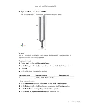
You can build up the fork geometry efficiently using predefined geometry primitives.
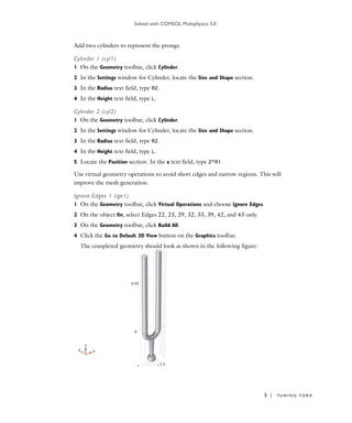
Cone 1 (cone1)
1 On the Geometry toolbar, click Cone.
Name Expression Value Description
L 7.8[cm] 0.078000 m Cylinder length
R1 7.5[mm] 0.0075000 m Base radius
R2 2.5[mm] 0.0025000 m Prong radius](https://image.slidesharecdn.com/models-150710220925-lva1-app6892/85/Models-mph-tuning-fork-3-320.jpg)
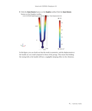


The document describes a model of a tuning fork used to tune musical instruments to a frequency of 440 Hz. It defines the geometry of the tuning fork using parameters like the prong radius and length. A finite element analysis is performed to calculate the fundamental eigenfrequency and mode shape by varying the prong length in a parametric sweep. The results show that a length of 0.0791 m produces an eigenfrequency closest to the desired 440 Hz frequency.


