Modeling and predicting the monthly rainfall in tamilnadu

International Journal of ComputerComputerand Technology (IJCET), ISSN 0976 – 6367(Print),
International Journal of Engineering Engineering
ISSN 0976 – 6375(Online) Volume 1, Number 1, May - June (2010), © IAEME
and Technology (IJCET), ISSN 0976 – 6367(Print) IJCET
ISSN 0976 – 6375(Online) Volume 1
Number 1, May - June (2010), pp. 103-111 ©IAEME
© IAEME, http://www.iaeme.com/ijcet.html

MODELING AND PREDICTING THE MONTHLY
RAINFALL IN TAMILNADU AS A SEASONAL
MULTIVARIATE ARIMA PROCESS
M. Nirmala
Research Scholar, Sathyabama University
Rajiv Gandhi Road, Jeppiaar Nagar, Chennai – 19
Email ID: monishram5002@gmail.com

S. M. Sundaram
Department of Mathematics, Sathyabama University
Rajiv Gandhi Road, Jeppiaar Nagar, Chennai – 19
Email ID: sundarambhu@rediffmail.com

ABSTRACT:
Amongst all weather happenings, rainfall plays the most imperative role in
human life. The understanding of rainfall variability helps the agricultural management in
planning and decision- making process. The important aspect of this research is to find a
suitable time series seasonal model for the prediction of the amount of rainfall in
Tamilnadu. In this study, Box-Jenkins model is used to build a Multivariate ARIMA
model for predicting the monthly rainfall in Tamilnadu together with a predictor, Sea
Surface Temperature for the period of 59 years (1950 – 2008) with a total of 708
readings.
Keywords: Seasonality, Sea Surface Temperature, Monthly Rainfall, Prediction,
Multivariate ARIMA
INTRODUCTION:
Time series analysis is an important tool in modeling and forecasting. Among the
most effective approaches for analyzing time series data is the model introduced by Box
and Jenkins [1], Autoregressive Integrated Moving Average (ARIMA). Box-Jenkins
ARIMA modeling has been successfully applied in various water and environmental

103

International Journal of Computer Engineering and Technology (IJCET), ISSN 0976 – 6367(Print),

management applications. The association between the southwest and northeast monsoon
rainfall over Tamilnadu have been examined for the 100 year period from 1877 – 1976
through a correlation analysis by O.N. Dhar and P.R. Rakhecha [2]. The average rainfall
series of Tamilnadu for the northeast monsoon months of October to December and the
season as a whole were analyzed for trends, periodicities and variability using standard
statistical methods by O. N. Dhar, P. R. Rakhecha, and A. K. Kulkarni [3]. Balachandran
S., Asokan R. and Sridharan S [4] examined the local and teleconnective association
between Northeast Monsoon Rainfall (NEMR) over Tamilnadu and global Surface
Temperature Anomalies (STA) using the monthly gridded STA data for the period 1901-
2004. The trends, periodicities and variability in the seasonal and annual rainfall series of
Tamilnadu were analyzed by O. N. Dhar, P. R. Rakhecha, and A. K. Kulkarni [5]. The
annual rainfall in Tamilnadu was predicted using a suitable Box – Jenkins ARIMA model
by M. Nirmala and S.M.Sundaram [6].

STUDY AREA AND MATERIALS:
Tamilnadu stretches between 8o 5'-13o 35' N by latitude and between 78o 18'-
80o 20' E by longitude. Tamilnadu is in the southeastern portion of the Deccan in India,
which extends from the Vindhya mountains in the north to Kanyakumari in the south.
Tamilnadu receives rainfall in both the southwest and northeast monsoon. Agriculture is
more dependants on the northeast monsoon. The rainfall during October to December
plays an important role in deciding the fate of the agricultural economy of the state.
Another important agro – climatic zone is the Cauvery river delta zone, which depends
on the southwest monsoon. Tamilnadu should normally receive 979 mm of rainfall every
year. Approximately 33% is from the southwest monsoon and 48 % is from the northeast
monsoon.

104


Figure 1 Geographical location of area of study, Tamilnadu
A dataset containing a total of 59 years (1950 - 2008) monthly rainfall totals of
Tamilnadu was obtained from Indian Institute of Tropical Meteorology (IITM), Pune,
India. The monthly Sea Surface Temperature of Nino 3.4 indices were obtained from
National Oceanic and Atmospheric Administration, United States, for a period of 59
years (1950 – 2008) with 708 observations.
METHODOLOGY:
BOX-JENKINS SEASONAL MULTIVARIATE ARIMA MODEL:

Univariate time series analysis using Box-Jenkins ARIMA model is a major tool
in hydrology and has been used extensively, mainly for the prediction of such surface
water processes as precipitation and stream flow events. It is basically a linear statistical
technique and most powerful for modeling the time series and rainfall forecasting due to
ease in its development and implementation. The ARIMA models are a combination of
autoregressive models and moving average models [1]. The autoregressive models AR(p)
base their predictions of the values of a variable xt, on a number p of past values of the

105


same variable number of autoregressive delays xt−1,xt−2,. . . xt−p and include a random
disturbance et. The moving average models MA(q) generate predictions of a variable xt
based on a number q of past disturbances of the same variable prediction errors of past
values et−1,et−2,. . ., et−q. The combination of the auto regressive and moving average
models AR(p) and MA(q) generates more flexible models called ARMA(p,q) models.
The stationarity of the time series is required for the implementation of all these models.
In 1976, Box and Jenkins proposed the mathematical transformation of the non-stationary
time series into stationary time series by a difference process defined by an order of
integration parameter d. This transforms ARMA (p,q) models for non stationary
transformed time series as the ARIMA (p,d,q) models.

The ARIMA model building strategy includes iterative identification, estimation,
diagnosis and forecasting stages [7]. Identification of a model may be accomplished on
the basis of the data pattern, time series plot and using their autocorrelation function and
partial autocorrelation function. The parameters are estimated and tested for statistical
significance after identifying the tentative model. If the parameter estimates does not
meet the stationarity condition then a new model should be identified and its parameters
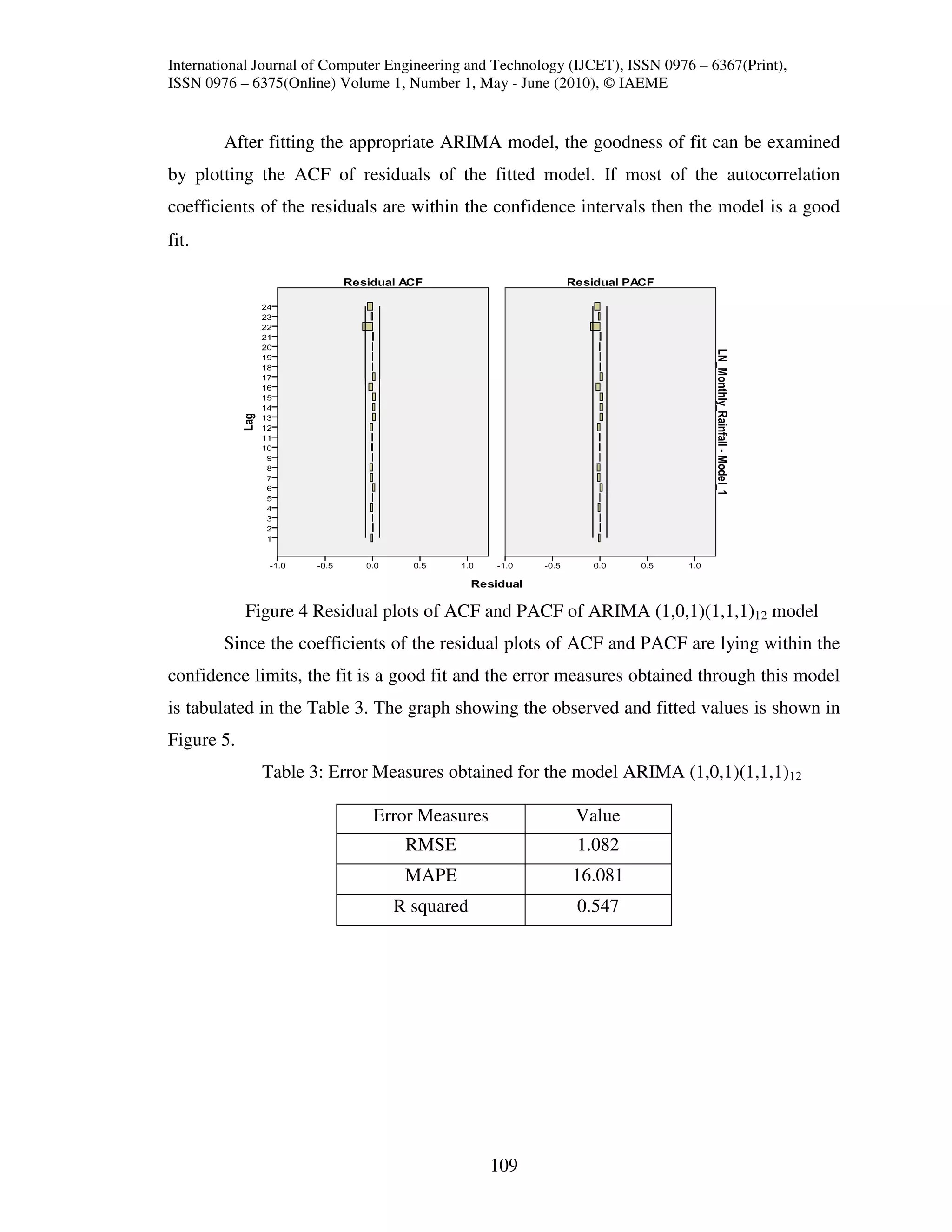
are estimated and tested. After finding the correct model it should be diagnosed. In the
diagnosis process, the autocorrelation of the residuals from the estimated model should
be sufficiently small and should resemble white noise. If the residuals remain
significantly correlated among themselves, a new model should be identified estimated
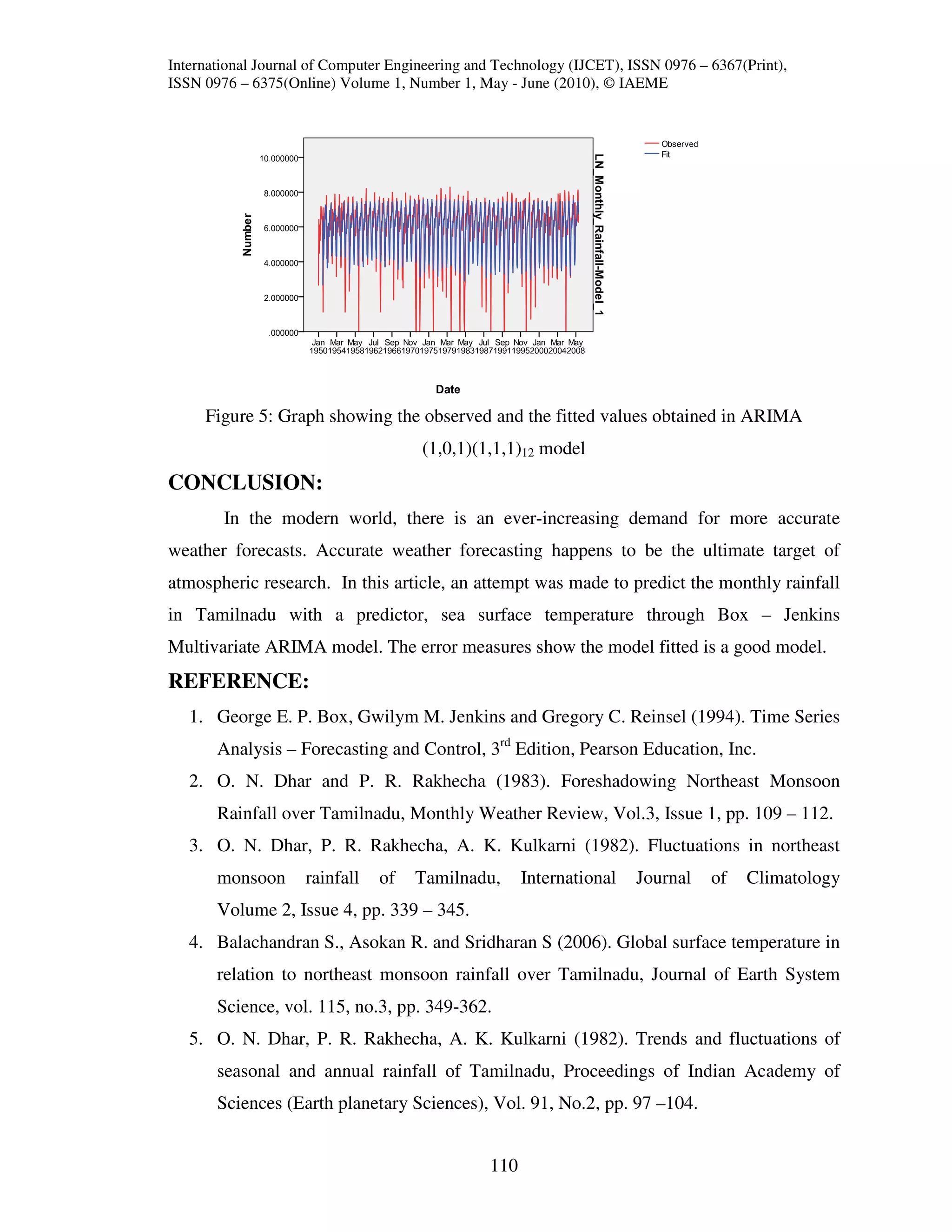
and diagnosed. Once the model is selected it is used to forecast the monthly rainfall
series. Time series analysis provides great opportunities for detecting, describing and
modeling climatic variability and impacts. Ultimately, to understand the meteorological
information and integrate it into planning and decision making process, it is important to
study the temporal characteristic and predict lead times of the rainfall of a region. This
can be done by identifying the best time series model using Box – Jenkins Seasonal
ARIMA modeling techniques. The Seasonal ARIMA (p,d,q)(P,D,Q)s model is defined as

φ p ( B)Φ P ( B s )∇ d ∇ s D yt = Θ Q ( B s )θ q ( B)ε t …………… [1]

106


Where

φ p ( B ) = 1 − φ1 B − ........... − φ p B p , θ q ( B ) = 1 − θ1 B − ............ − θ q B q
…..[2]
Φ P ( B s ) = 1 − Φ 1 B s − ........ − Φ P B sP , Θ Q ( B s ) = 1 − Θ1 B s − ....... − Θ Q B sQ

εt denotes the error term, φ’s and Φ’s are the non seasonal and seasonal autoregressive
parameters and θ’s and Θ’s are the non seasonal and seasonal moving average
parameters.
RESULTS AND DISCUSSIONS:
A time series is said to be stationary if its underlying generating process is based
on constant mean and constant variance with its autocorrelation function (ACF)
essentially constant through time. The ACF is a measure of the correlation between two
variables composing the stochastic process, which are k temporal lags far away and the
Partial Autocorrelation Function (PACF) measures the net correlation between two
variables, which are k temporal lags far away.

TIME SERIES POLT OF MONTHLY RAINFALL IN TAMILNADU

4500
MONTHLY RAINFALL

4000
3500
3000
2500
2000
1500
1000
500
0
1
34
67
100
133
166
199
232
265
298
331
364
397
430
463
496
529
562
595
628
661
694

MONTH

Figure 2 Time Series Plot of Monthly Rainfall in Tamilnadu (1950 - 2008)
The visual plot of the time series plot (Figure 2) is often enough to convince a
statistician that the series is stationary or non – stationary [6]. The visual inspection of
the sample autocorrelation function shows that the rainfall series is stationary. If the
Autocorrelation function dies out rapidly, that is, it reaches zero within one or two lag
periods then it indicates that the time series is stationary. From the pattern of ACF and
PACF plots, the monthly rainfall series is stationary but with seasonality.

107


Figure 3 ACF and PACF correlograms
Seasonality is defined as a pattern that repeats itself over fixed intervals of times.
For a stationary data, seasonality can be found by identifying those autocorrelation
coefficients of more than two or three time lags that are significantly different from zero
[8]. Since the monthly rainfall series consists seasonality of order s = 12, the model
considered here is a seasonal multivariate ARIMA model.
Table 1: ACF and PACF coefficients for the first five lags
Lag ACF coefficient PACF coefficient
1 0.457 0.457
2 0.123 -0.108
3 -0.155 -0.215
4 -0.268 -0.127
5 -0.250 -0.069

The ACF and PACF correlograms (figure 3) and the coefficients are analyzed
carefully and the tentative multivariate ARIMA model chosen is ARIMA (1,0,1)(1,1,1)12.
The parameter’s estimates are tabulated in table 2.
Table 2: Parameter’s Estimates of ARIMA (1,0,1)(1,1,1)12 model
Model Parameters Parameter’s
Estimates
ARIMA AR 0.475
(1,0,1)(1,1,1)12 MA 0.392
AR, Seasonal 0.072
MA, Seasonal 0.965

108


After fitting the appropriate ARIMA model, the goodness of fit can be examined
by plotting the ACF of residuals of the fitted model. If most of the autocorrelation
coefficients of the residuals are within the confidence intervals then the model is a good
fit.

Figure 4 Residual plots of ACF and PACF of ARIMA (1,0,1)(1,1,1)12 model
Since the coefficients of the residual plots of ACF and PACF are lying within the
confidence limits, the fit is a good fit and the error measures obtained through this model
is tabulated in the Table 3. The graph showing the observed and fitted values is shown in
Figure 5.
Table 3: Error Measures obtained for the model ARIMA (1,0,1)(1,1,1)12

Error Measures Value
RMSE 1.082
MAPE 16.081
R squared 0.547

109


Figure 5: Graph showing the observed and the fitted values obtained in ARIMA
(1,0,1)(1,1,1)12 model
CONCLUSION:
In the modern world, there is an ever-increasing demand for more accurate
weather forecasts. Accurate weather forecasting happens to be the ultimate target of
atmospheric research. In this article, an attempt was made to predict the monthly rainfall
in Tamilnadu with a predictor, sea surface temperature through Box – Jenkins
Multivariate ARIMA model. The error measures show the model fitted is a good model.
REFERENCE:
1. George E. P. Box, Gwilym M. Jenkins and Gregory C. Reinsel (1994). Time Series
Analysis – Forecasting and Control, 3rd Edition, Pearson Education, Inc.
2. O. N. Dhar and P. R. Rakhecha (1983). Foreshadowing Northeast Monsoon
Rainfall over Tamilnadu, Monthly Weather Review, Vol.3, Issue 1, pp. 109 – 112.
3. O. N. Dhar, P. R. Rakhecha, A. K. Kulkarni (1982). Fluctuations in northeast
monsoon rainfall of Tamilnadu, International Journal of Climatology
Volume 2, Issue 4, pp. 339 – 345.
4. Balachandran S., Asokan R. and Sridharan S (2006). Global surface temperature in
relation to northeast monsoon rainfall over Tamilnadu, Journal of Earth System
Science, vol. 115, no.3, pp. 349-362.
5. O. N. Dhar, P. R. Rakhecha, A. K. Kulkarni (1982). Trends and fluctuations of
seasonal and annual rainfall of Tamilnadu, Proceedings of Indian Academy of
Sciences (Earth planetary Sciences), Vol. 91, No.2, pp. 97 –104.

110


6. Nirmala M and Sundaram S.M. (2009), Rainfall Predicting Model: An Application
to Tamilnadu Rainfall Series, Proceedings of National Conference on Effect of
Climatic Change and Sustainable Resource Management, SRM University, and
Meteorological Department, Chennai India.
7. Damodar N. Gujarati and Sangeetha (2007). Basic Econometrics, 4th edition, the
Tata Mcgraw – Hill Publishing Company Limited.
8. Meaza Demissie (2003). Characterizing trends and identification of rainfall
predicting model: An application to Melksa observatory Nazreth rainfall series,
Proceedings of Biometric society, pp.132 – 134.
9. Nirmala M and Sundaram S.M. (2010), Comparison of Learning Algorithms with
the ARIMA Model for the Forecasting of Annual Rainfall in Tamilnadu,
International Journal on Information Sciences and Computing, Vol.4, No.1,
pp.64 – 71.

111

Modeling and predicting the monthly rainfall in tamilnadu

More Related Content

What's hot

Viewers also liked

Similar to Modeling and predicting the monthly rainfall in tamilnadu

More from iaemedu

Modeling and predicting the monthly rainfall in tamilnadu