Download to read offline
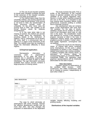
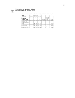
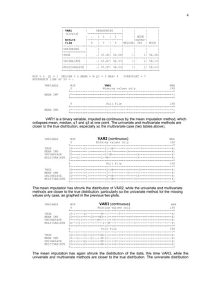
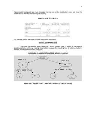
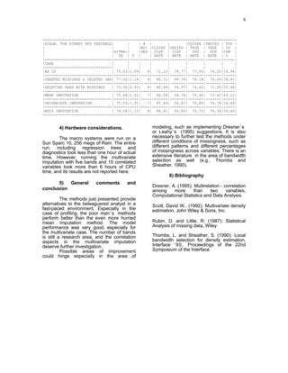

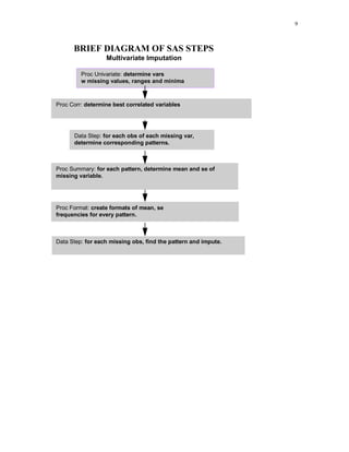

1) The document describes a method for imputing missing values in large multivariate databases. It proposes modeling variables on bins to address the curse of dimensionality. Variables are selected based on correlation and those with overlapping missingness are excluded. Values are imputed sequentially based on patterns in other variables. 2) Potential improvements discussed include using more sophisticated modeling methods, addressing increased variances from using imputed variables, and handling non-random missingness. 3) An empirical application imputes missing ages in a customer database using various methods. Results show the multivariate method best matches the true distribution of a binary variable compared to mean imputation or deleting missing cases.