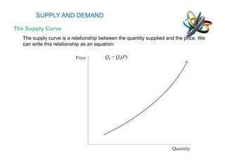
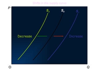
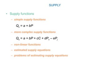
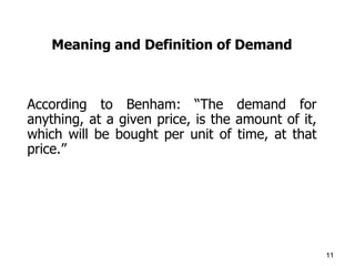
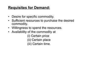
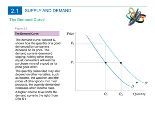
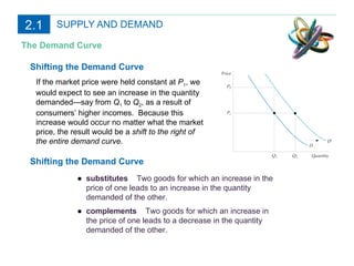
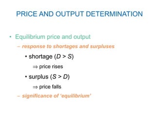
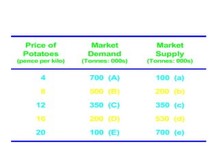
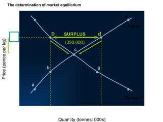
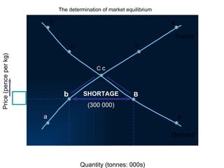
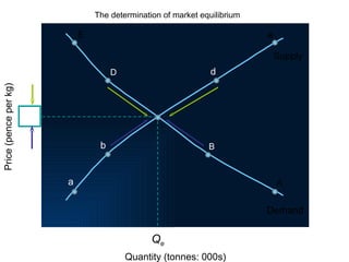
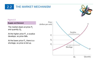
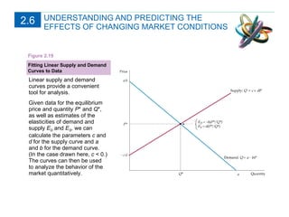
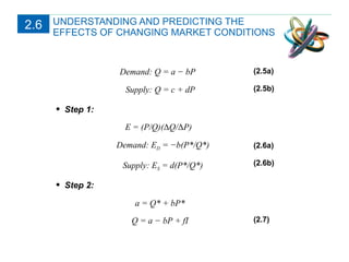
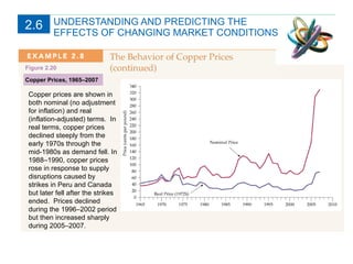
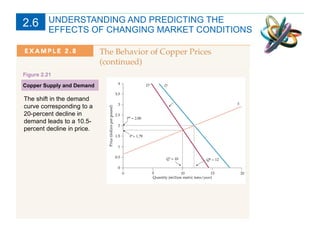
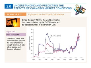
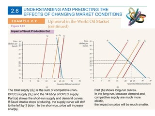
SlideShare a Scribd company logo
Supply and Demand
OUTLINE 2.1 Supply and Demand 2.2 The Market Mechanism 2.3 Changes in Market Equilibrium 2.4 Elasticities of Supply and Demand 2.5 Short-Run versus Long-Run Elasticities 2.6 Understanding and Predicting the Effects of Changing Market Conditions 2.7 Effects of Government Intervention—Price Controls
The Basics of Supply and Demand ,[object Object],[object Object],[object Object],Supply-demand analysis is a fundamental and powerful tool that can be applied to a wide variety of interesting and important problems. To name a few:
SUPPLY AND DEMAND ,[object Object],The supply curve is a relationship between the quantity supplied and the price. We can write this relationship as an equation: Q S  =  Q S ( P )
SUPPLY AND DEMAND ,[object Object],● supply curve  Relationship between the quantity of a good that producers are willing to sell and the price of the good. The Supply Curve The supply curve, labeled  S  in the figure, shows how the quantity of a good offered for sale changes as the price of the good changes. The supply curve is upward sloping: The higher the price, the more firms are able and willing to produce and sell.  If production costs fall, firms can produce the same quantity at a lower price or a larger quantity at the same price. The supply curve then shifts to the right (from  S  to  S’ ). Figure 2.1
SUPPLY ,[object Object],[object Object],[object Object],[object Object],[object Object],[object Object],[object Object],[object Object]
SUPPLY ,[object Object],[object Object],[object Object],[object Object],[object Object],[object Object],[object Object]
P Q O S 0 Increase Shifts in the supply curve S 1
P Q O S 0 S 1 Increase Decrease Shifts in the supply curve S 2
SUPPLY ,[object Object],[object Object],[object Object],[object Object],[object Object],[object Object],[object Object],[object Object]
Meaning and Definition of Demand According to Benham: “The demand for anything, at a given price, is the amount of it, which will be bought per unit of time, at that price.”
[object Object],[object Object],[object Object],[object Object],[object Object],[object Object],[object Object],[object Object]
Factors Determining Demand ,[object Object],[object Object],[object Object],[object Object],[object Object],[object Object],[object Object],[object Object],[object Object]
SUPPLY AND DEMAND ,[object Object],We can write this relationship between quantity demanded and price as an equation: Q D  =  Q D ( P ) ● demand curve  Relationship between the quantity of a good that consumers are willing to buy and the price of the good. 2.1
Market demand for potatoes (monthly) Quantity (tonnes: 000s) Price (pence per kg) Price (pence per kg) 20 40 60  80  100   Market demand (tonnes 000s ) 700 500 350 200 100 A B C D E Point A B C D E Demand
Change in Demand ,[object Object],[object Object],[object Object],[object Object],[object Object],[object Object],[object Object]
Shift in the Demand Curve ,[object Object]
[object Object],[object Object],[object Object],[object Object],[object Object],[object Object],[object Object]
SUPPLY AND DEMAND ,[object Object],The Demand Curve The demand curve, labeled  D,  shows how the quantity of a good demanded by consumers depends on its price. The demand curve is downward sloping; holding other things equal, consumers will want to purchase more of a good as its price goes down.  The quantity demanded may also depend on other variables, such as income, the weather, and the prices of other goods. For most products, the quantity demanded increases when income rises.  A higher income level shifts the demand curve to the right (from  D  to  D’ ). Figure 2.2 2.1
SUPPLY AND DEMAND ,[object Object],Shifting the Demand Curve If the market price were held constant at  P 1 , we would expect to see an increase in the quantity demanded—say from  Q 1  to  Q 2 , as a result of consumers’ higher incomes.  Because this increase would occur no matter what the market price, the result would be a  shift to the right of the entire demand curve. Shifting the Demand Curve ● substitutes  Two goods for which an increase in the price of one leads to an increase in the quantity demanded of the other. ● complements  Two goods for which an increase in the price of one leads to a decrease in the quantity demanded of the other. 2.1
PRICE AND OUTPUT DETERMINATION ,[object Object],[object Object],[object Object],[object Object],[object Object],[object Object],[object Object]
Equilibrium price and output: The Market Demand and Supply of Potatoes (Monthly)
The determination of market equilibrium   Quantity (tonnes: 000s) E C B A a b c e Supply Demand Price (pence per kg) D d SURPLUS (330 000)
The determination of market equilibrium   Quantity (tonnes: 000s) E D C B A a b c d e Supply Demand Price (pence per kg) SHORTAGE (300 000)
The determination of market equilibrium   D d Q e Quantity (tonnes: 000s) E B A a b e Supply Demand Price (pence per kg)
THE MARKET MECHANISM Supply and Demand The market clears at price  P 0  and quantity  Q 0 .  At the higher price  P 1 , a surplus develops, so price falls.  At the lower price  P 2 , there is a shortage, so price is bid up. Figure 2.3 2.2
THE MARKET MECHANISM Equilibrium ● equilibrium ( or  market clearing) price  Price that equates the quantity supplied to the quantity demanded. ● market mechanism  Tendency in a free market for price to change until the market clears. ● surplus  Situation in which the quantity supplied exceeds the quantity demanded. ●   shortage  Situation in which the quantity demanded exceeds the quantity supplied. 2.2
THE MARKET MECHANISM When Can We Use the Supply-Demand Model? We are assuming that at any given price, a given quantity will be produced and sold. This assumption makes sense only if a market is at least roughly  competitive . By this we mean that both sellers and buyers should have little  market power —i.e., little ability  individually  to affect the market price. Suppose instead that supply were controlled by a single producer—a monopolist. If the demand curve shifts in a particular way, it may be in the monopolist’s interest to keep the quantity fixed but change the price, or to keep the price fixed and change the quantity. 2.2
CHANGES IN MARKET EQUILIBRIUM New Equilibrium Following  Shift in Supply When the supply curve shifts to the right, the market clears at a lower price  P 3  and a larger quantity  Q 3 . Figure 2.4 2.3
CHANGES IN MARKET EQUILIBRIUM New Equilibrium Following Shift in Demand When the demand curve shifts to the right, the market clears at a higher price  P 3  and a larger quantity  Q 3 . Figure 2.5 2.3
CHANGES IN MARKET EQUILIBRIUM New Equilibrium Following Shifts in Supply and Demand Supply and demand curves shift over time as market conditions change.  In this example, rightward shifts of the supply and demand curves lead to a slightly higher price and a much larger quantity.  In general, changes in price and quantity depend on the amount by which each curve shifts and the shape of each curve. Figure 2.6 2.3
REAL VERSUS NOMINAL PRICES The real price of eggs in  1970   dollars  is calculated as follows: Table 1.1  The Real Price of Eggs and of a College Education 1970 1980 1990 2000 2007 Consumer Price Index 38.8 82.4 130.7 172.2 205.8 Nominal Prices Grade A Large Eggs $0.61 $0.84 $1.01 $0.91 $1.64 College Education $2,530 $4,912 $12,018 $20,186 $27,560 Real Prices ($1970) Grade A Large Eggs $0.61 $0.40 $0.30 $0.21 $0.31 College Education $2,530 $2,313 $3,568 $4,548 $5,196 1.3
REAL VERSUS NOMINAL PRICES The real price of eggs in  1990   dollars  is calculated as follows: $5,196 $4,548 $3,568 $2,313 $2,530 College Education $1.04 $0.69 $1.01 $1.33 $2.05 Grade A Large Eggs The Real Price of Eggs and of a College Education (continued) 1970 1980 1990 2000 2007 Consumer Price Index 38.8 82.4 130.7 172.2 205.8 Nominal Prices Grade A Large Eggs $0.61 $0.84 $1.01 $0.91 $1.64 College Education $2,530 $4,912 $12,018 $20,186 $27,560 Real Prices ($1980) 1.3
REAL VERSUS NOMINAL PRICES The percentage change in real price is calculated as follows: $5,196 $4,548 $3,568 $2,313 $2,530 College Education $1.04 $0.69 $1.01 $1.33 $2.05 Grade A Large Eggs The Real Price of Eggs and of a College Education (continued) 1970 1980 1990 2000 2007 Consumer Price Index 38.8 82.4 130.7 172.2 205.8 Nominal Prices Grade A Large Eggs $0.61 $0.84 $1.01 $0.91 $1.64 College Education $2,530 $4,912 $12,018 $20,186 $27,560 Real Prices ($1980) 1.3
CHANGES IN MARKET EQUILIBRIUM From 1970 to 2007, the real (constant-dollar) price of eggs fell by 49 percent, while the real price of a college education rose by 105 percent. The mechanization of poultry farms sharply reduced the cost of producing eggs, shifting the supply curve downward. The demand curve for eggs shifted to the left as a more health-conscious population tended to avoid eggs. As for college, increases in the costs of equipping and maintaining modern classrooms, laboratories, and libraries, along with increases in faculty salaries, pushed the supply curve up. The demand curve shifted to the right as a larger percentage of a growing number of high school graduates decided that a college education was essential. 2.3
CHANGES IN MARKET EQUILIBRIUM (a) Market for Eggs The supply curve for eggs shifted downward as production costs fell; the demand curve shifted to the left as consumer preferences changed.  As a result, the real price of eggs fell sharply and egg consumption rose. Figure 2.7 2.3
CHANGES IN MARKET EQUILIBRIUM (b) Market for College Education The supply curve for a college education shifted up as the costs of equipment, maintenance, and staffing rose.  The demand curve shifted to the right as a growing number of high school graduates desired a college education.  As a result, both price and enrollments rose sharply. Figure 2.7 2.3
CHANGES IN MARKET EQUILIBRIUM Over the past two decades, the wages of skilled high-income workers have grown substantially, while the wages of unskilled low-income workers have fallen slightly. From 1978 to 2005, people in the top 20 percent of the income distribution experienced an increase in their average real (inflation-adjusted) pretax household income of 50 percent, while those in the bottom 20 percent saw their average real pretax income increase by only 6 percent. While the supply of unskilled workers—people with limited  educations—has grown substantially, the demand for them has risen only slightly. On the other hand, while the supply of skilled workers—e.g., engineers, scientists, managers, and economists—has grown slowly, the demand has risen dramatically, pushing wages up. 2.3
CHANGES IN MARKET EQUILIBRIUM Consumption and the Price of Copper Although annual consumption of copper has increased about a hundredfold,  the real (inflation-adjusted) price has not changed much. Figure 2.8 2.3
CHANGES IN MARKET EQUILIBRIUM Long-Run Movements of Supply and Demand for Mineral Resources Although demand for most resources has increased dramatically over the past century, prices have fallen or risen only slightly in real (inflation-adjusted) terms because cost reductions have shifted the supply curve to the right just as dramatically. Figure 2.9 2.3
CHANGES IN MARKET EQUILIBRIUM Supply and Demand for New York City Office Space Following 9/11 the supply curve shifted to the left, but the demand curve also shifted to the left, so that the average rental price fell. Figure 2.10 2.3
ELASTICITIES OF SUPPLY AND DEMAND ,[object Object],[object Object],[object Object],(2.1) 2.4
ELASTICITIES OF SUPPLY AND DEMAND ,[object Object],[object Object],Linear Demand Curve Figure 2.11 The price elasticity of demand depends not only on the slope of the demand curve but also on the price and quantity. The elasticity, therefore, varies along the curve as price and quantity change. Slope is constant for this linear demand curve.  Near the top, because price is high and quantity is small, the elasticity is large in magnitude.  The elasticity becomes smaller as we move down the curve. 2.4
ELASTICITIES OF SUPPLY AND DEMAND ,[object Object],[object Object],(a) Infinitely Elastic Demand Figure 2.12 (a)  For a horizontal demand curve,  ΔQ/ΔP  is infinite. Because a tiny change in price leads to an enormous change in demand, the elasticity of demand is infinite. 2.4
ELASTICITIES OF SUPPLY AND DEMAND ,[object Object],[object Object],(b) Completely Inelastic Demand Figure 2.12 (b)  For a vertical demand curve,  ΔQ/ΔP  is zero.  Because the quantity demanded is the same no matter what the price, the elasticity of demand is zero. 2.4
ELASTICITIES OF SUPPLY AND DEMAND ,[object Object],[object Object],[object Object],[object Object],Elasticities of Supply (2.2) (2.3) 2.4
ELASTICITIES OF SUPPLY AND DEMAND ,[object Object],[object Object],[object Object],Arc Elasticity of Demand (2.4) 2.4
ELASTICITIES OF SUPPLY AND DEMAND During recent decades, changes in the wheat market had major implications for both American farmers and U.S. agricultural policy. To understand what happened, let’s examine the behavior of supply and demand beginning in 1981. By setting the quantity supplied equal to the quantity demanded, we can determine the market-clearing price of wheat for 1981: 2.4
ELASTICITIES OF SUPPLY AND DEMAND Substituting into the supply curve equation, we get We use the demand curve to find the price elasticity of demand: We can likewise calculate the price elasticity of supply: Because these supply and demand curves are linear, the price elasticities will vary as we move along the curves. Thus demand is inelastic. 2.4
[object Object],SHORT-RUN VERSUS LONG-RUN ELASTICITIES (a) Gasoline: Short-Run and Long-Run Demand Curves Figure 2.13 (a)  In the short run, an increase in price has only a small effect on the quantity of gasoline demanded. Motorists may drive less, but they will not change the kinds of cars they are driving overnight.  In the longer run, however, because they will shift to smaller and more fuel-efficient cars, the effect of the price increase will be larger. Demand, therefore, is more elastic in the long run than in the short run. 2.5
[object Object],SHORT-RUN VERSUS LONG-RUN ELASTICITIES (b) Automobiles: Short-Run and Long-Run Demand Curves Figure 2.13 (b)  The opposite is true for automobile demand. If price increases, consumers initially defer buying new cars; thus annual quantity demanded falls sharply.  In the longer run, however, old cars wear out and must be replaced; thus annual quantity demanded picks up. Demand, therefore, is less elastic in the long run than in the short run. Demand and Durability 2.5
[object Object],SHORT-RUN VERSUS LONG-RUN ELASTICITIES Income Elasticities Income elasticities also differ from the short run to the long run. For most goods and services—foods, beverages, fuel, entertainment, etc.— the income elasticity of demand is larger in the long run than in the short run. For a durable good, the opposite is true. The short-run income elasticity of demand will be much larger than the long-run elasticity. 2.5
[object Object],SHORT-RUN VERSUS LONG-RUN ELASTICITIES GDP and Investment in Durable Equipment Figure 2.14 Annual growth rates are compared for GDP and investment in durable equipment.  Because the short-run GDP elasticity of demand is larger than the long-run elasticity for long-lived capital equipment, changes in investment in equipment magnify changes in GDP. Thus capital goods industries are considered “cyclical.” Cyclical Industries ,[object Object],2.5
[object Object],SHORT-RUN VERSUS LONG-RUN ELASTICITIES Consumption of Durables versus Nondurables Figure 2.15 Annual growth rates are compared for GDP, consumer expenditures on durable goods (automobiles, appliances, furniture, etc.), and consumer expenditures on nondurable goods (food, clothing, services, etc.).  Because the stock of durables is large compared with annual demand, short-run demand elasticities are larger than long-run elasticities. Like capital equipment, industries that produce consumer durables are “cyclical” (i.e., changes in GDP are magnified). This is not true for producers of nondurables. Cyclical Industries 2.5
[object Object],SHORT-RUN VERSUS LONG-RUN ELASTICITIES 2.5 TABLE 2.1  Demand for Gasoline Number of Years Allowed to Pass Following a Price or Income Change Elasticity  1  2  3  5  10 Price  −0.2  −0.3  −0.4  −0.5  −0.8 Income    0.2    0.4    0.5  0.6  1.0 TABLE 2.2  Demand for Automobiles Number of Years Allowed to Pass Following a Price or Income Change Elasticity  1  2  3  5  10 Price  −1.2  −0.9  −0.8  −0.6  −0.4 Income  3.0  2.3  1.9  1.4  1.0
[object Object],SHORT-RUN VERSUS LONG-RUN ELASTICITIES Supply and Durability Copper: Short-Run and Long-Run Supply Curves Figure 2.16 Like that of most goods, the supply of primary copper, shown in part  (a) , is more elastic in the long run.  If price increases, firms would like to produce more but are limited by capacity constraints in the short run. In the longer run, they can add to capacity and produce more. 2.5
[object Object],SHORT-RUN VERSUS LONG-RUN ELASTICITIES Supply and Durability Copper: Short-Run and Long-Run Supply Curves Figure 2.16 Part  (b)  shows supply curves for secondary copper.  If the price increases, there is a greater incentive to convert scrap copper into new supply. Initially, therefore, secondary supply (i.e., supply from scrap) increases sharply. But later, as the stock of scrap falls, secondary supply contracts.  Secondary supply is therefore less elastic in the long run than in the short run. 2.5 Table 2.3  Supply of Copper Price Elasticity of:  Short-Run  Long-Run Primary supply 0.20 1.60 Secondary supply 0.43 0.31 Total supply 0.25 1.50
SHORT-RUN VERSUS LONG-RUN ELASTICITIES Price of Brazilian Coffee Figure 2.17 When droughts or freezes damage Brazil’s coffee trees, the price of coffee can soar. The price usually falls again after a few years, as demand and supply adjust. 2.5
SHORT-RUN VERSUS LONG-RUN ELASTICITIES Supply and Demand for Coffee Figure 2.18 (a)  A freeze or drought in Brazil causes the supply curve to shift to the left.  In the short run, supply is completely inelastic; only a fixed number of coffee beans can be harvested.  Demand is also relatively inelastic; consumers change their habits only slowly.  As a result, the initial effect of the freeze is a sharp increase in price, from  P 0  to  P 1 . 2.5
SHORT-RUN VERSUS LONG-RUN ELASTICITIES Supply and Demand for Coffee Figure 2.18 (b)  In the intermediate run, supply and demand are both more elastic; thus price falls part of the way back, to  P 2 . 2.5
SHORT-RUN VERSUS LONG-RUN ELASTICITIES Supply and Demand for Coffee Figure 2.18 (c)  In the long run, supply is extremely elastic; because new coffee trees will have had time to mature, the effect of the freeze will have disappeared. Price returns to  P 0 . 2.5
UNDERSTANDING AND PREDICTING THE  EFFECTS OF CHANGING MARKET CONDITIONS Fitting Linear Supply and Demand Curves to Data Figure 2.19 Linear supply and demand  curves provide a convenient tool for analysis.  Given data for the equilibrium price and quantity  P * and  Q *, as well as estimates of the elasticities of demand and supply  E D  and  E S , we can calculate the parameters  c  and  d  for the supply curve and  a  and  b  for the demand curve. (In the case drawn here,  c  < 0.) The curves can then be used to analyze the behavior of the market quantitatively. 2.6
UNDERSTANDING AND PREDICTING THE  EFFECTS OF CHANGING MARKET CONDITIONS ,[object Object],[object Object],Demand: Q = a − bP Supply: Q = c + dP E = (P/Q)( Δ Q/ Δ P) Demand: E D   = −b(P*/Q*) Supply: E S   = d(P*/Q*) a = Q* + bP* Q = a − bP + fI (2.5a) (2.5b) (2.6a) (2.6b) (2.7) 2.6
UNDERSTANDING AND PREDICTING THE  EFFECTS OF CHANGING MARKET CONDITIONS After reaching a level of about $1.00 per pound in 1980, the price of copper fell sharply to about 60 cents per pound in 1986. Worldwide recessions in 1980 and 1982 contributed to the decline of copper prices. Why did the price increase sharply in 2005–2007? First, the demand for copper from China and other Asian countries began increasing dramatically. Second, because prices had dropped so much from 1996 through 2003, producers closed unprofitable mines and cut production. What would a decline in demand do to the price of copper? To find out, we can use linear supply and demand curves. 2.6
UNDERSTANDING AND PREDICTING THE  EFFECTS OF CHANGING MARKET CONDITIONS Copper prices are shown in both nominal (no adjustment for inflation) and real (inflation-adjusted) terms.  In real terms, copper prices declined steeply from the early 1970s through the mid-1980s as demand fell. In 1988–1990, copper prices rose in response to supply disruptions caused by strikes in Peru and Canada but later fell after the strikes ended.  Prices declined during the 1996–2002 period but then increased sharply during 2005–2007. Copper Prices, 1965–2007 Figure 2.20 2.6
UNDERSTANDING AND PREDICTING THE  EFFECTS OF CHANGING MARKET CONDITIONS Copper Supply and Demand Figure 2.21 The shift in the demand curve corresponding to a 20-percent decline in demand leads to a 10.5-percent decline in price. 2.6
UNDERSTANDING AND PREDICTING THE  EFFECTS OF CHANGING MARKET CONDITIONS Price of Crude Oil Figure 2.22 The OPEC cartel and political events caused the price of oil to rise sharply at times. It later fell as supply and demand adjusted. Since the early 1970s, the world oil market has been buffeted by the OPEC cartel and by political turmoil in the Persian Gulf. 2.6
UNDERSTANDING AND PREDICTING THE  EFFECTS OF CHANGING MARKET CONDITIONS ,[object Object],[object Object],[object Object],[object Object],[object Object],[object Object],2.6 Short Run Long Run World demand: Competitive supply: -0.05 -0.40 0.10 0.40
UNDERSTANDING AND PREDICTING THE  EFFECTS OF CHANGING MARKET CONDITIONS Impact of Saudi Production Cut The total supply ( S T ) is the sum of competitive (non-OPEC) supply ( S C ) and the 14 bb/yr of OPEC supply.  Part (a) shows the short-run supply and demand curves. If Saudi Arabia stops producing, the supply curve will shift to the left by 3 bb/yr.  In the short-run, price will increase sharply. Figure 2.23 Part (b) shows long-run curves. In the long run, because demand and competitive supply are much more elastic,  the impact on price will be much smaller. 2.6
EFFECTS OF GOVERNMENT INTERVENTION— PRICE CONTROLS Effects of Price Controls Without price controls, the market clears at the equilibrium price and quantity  P 0  and  Q 0 .  If price is regulated to be no higher than  P max , the quantity supplied falls to  Q 1 , the quantity demanded increases to  Q 2 , and a shortage develops. Figure 2.24 2.7
EFFECTS OF GOVERNMENT INTERVENTION— PRICE CONTROLS Natural gas prices rose sharply after 2000, as did the prices of oil and other fuels. Price of Natural Gas Figure 2.25 2.7
EFFECTS OF GOVERNMENT INTERVENTION— PRICE CONTROLS ,[object Object],[object Object],[object Object],Supply:  Q  = 15.90 + 0.72 P G  + 0.05 P O Demand:  Q  = 0.02 – 0.18 P G  + 0.69 P O Substitute $3.00 for  P G  in both the supply and demand equations (keeping the price of oil,  P O , fixed at $50).  You should find that the supply equation gives a quantity supplied of 20.6 Tcf and the demand equation a quantity demanded of 29.1 Tcf.  Therefore, these price controls would create an excess demand of  29.1 − 20.6 = 8.5 Tcf. 2.7

More Related Content

What's hot

Supply Micro Economics ECO101
Supply Micro Economics ECO101Supply Micro Economics ECO101
Supply Micro Economics ECO101
Sabih Kamran
 
Demand, supply and equilibrium
Demand, supply and equilibriumDemand, supply and equilibrium
Demand, supply and equilibrium
Daud Dahir
 
The Market Forces of Supply and Demand
The Market Forces of Supply and DemandThe Market Forces of Supply and Demand
The Market Forces of Supply and Demand
Tuul Tuul
 
Demand and supply .ppt
Demand and supply .pptDemand and supply .ppt
Demand and supply .ppt
jaganshettar
 
Demand and Supply Analysis (Economics) Lecture Notes
Demand and Supply Analysis (Economics) Lecture NotesDemand and Supply Analysis (Economics) Lecture Notes
Demand and Supply Analysis (Economics) Lecture Notes
FellowBuddy.com
 
LAW OF SUPPLY AND DEMAND
LAW OF SUPPLY AND DEMANDLAW OF SUPPLY AND DEMAND
LAW OF SUPPLY AND DEMAND
Cheldy S, Elumba-Pableo
 
Elements of Demand and Supply
Elements of Demand and SupplyElements of Demand and Supply
Elements of Demand and Supply
Gregar Donaven Valdehueza
 
Supply ppt
Supply pptSupply ppt
Supply ppt
vivek_kasana
 
Supply and demand
Supply and demandSupply and demand
Supply and demand
gaurav jaiswal
 
Demand and supply presentation
Demand and supply presentationDemand and supply presentation
Demand and supply presentation
Sheeraz Latif
 
Chapter 3 - An Introduction to Demand and Supply.ppt
Chapter 3 - An Introduction to Demand and Supply.pptChapter 3 - An Introduction to Demand and Supply.ppt
Chapter 3 - An Introduction to Demand and Supply.ppt
ChelseaAnneVidallo
 
Elasticity Of Supply And Demand
Elasticity Of Supply And DemandElasticity Of Supply And Demand
Elasticity Of Supply And Demand
Kevin A
 
Supply & Elasticity of Supply.
Supply & Elasticity of Supply.Supply & Elasticity of Supply.
Supply & Elasticity of Supply.
KVS
 
The theory of supply
The theory of supply The theory of supply
The theory of supply
Akarsh Trivedi
 
a. elasticity of demand
 a. elasticity of demand a. elasticity of demand
a. elasticity of demand
Raunak Khinwasra
 
Price Elasticity of Supply
Price Elasticity of SupplyPrice Elasticity of Supply
Price Elasticity of Supply
tutor2u
 
ELASTICITY OF DEMAND
ELASTICITY  OF DEMANDELASTICITY  OF DEMAND
ELASTICITY OF DEMAND
Rohan Ranjane
 
Law of demand
Law of demand Law of demand
Law of demand
Michael Alonzo
 
Individual and Market Supply
Individual and Market SupplyIndividual and Market Supply
Individual and Market Supply
tutor2u
 

What's hot (20)

Supply Micro Economics ECO101
Supply Micro Economics ECO101Supply Micro Economics ECO101
Supply Micro Economics ECO101
 
Demand, supply and equilibrium
Demand, supply and equilibriumDemand, supply and equilibrium
Demand, supply and equilibrium
 
The Market Forces of Supply and Demand
The Market Forces of Supply and DemandThe Market Forces of Supply and Demand
The Market Forces of Supply and Demand
 
Demand and supply .ppt
Demand and supply .pptDemand and supply .ppt
Demand and supply .ppt
 
Demand and Supply Analysis (Economics) Lecture Notes
Demand and Supply Analysis (Economics) Lecture NotesDemand and Supply Analysis (Economics) Lecture Notes
Demand and Supply Analysis (Economics) Lecture Notes
 
Changes in demand
Changes in demandChanges in demand
Changes in demand
 
LAW OF SUPPLY AND DEMAND
LAW OF SUPPLY AND DEMANDLAW OF SUPPLY AND DEMAND
LAW OF SUPPLY AND DEMAND
 
Elements of Demand and Supply
Elements of Demand and SupplyElements of Demand and Supply
Elements of Demand and Supply
 
Supply ppt
Supply pptSupply ppt
Supply ppt
 
Supply and demand
Supply and demandSupply and demand
Supply and demand
 
Demand and supply presentation
Demand and supply presentationDemand and supply presentation
Demand and supply presentation
 
Chapter 3 - An Introduction to Demand and Supply.ppt
Chapter 3 - An Introduction to Demand and Supply.pptChapter 3 - An Introduction to Demand and Supply.ppt
Chapter 3 - An Introduction to Demand and Supply.ppt
 
Elasticity Of Supply And Demand
Elasticity Of Supply And DemandElasticity Of Supply And Demand
Elasticity Of Supply And Demand
 
Supply & Elasticity of Supply.
Supply & Elasticity of Supply.Supply & Elasticity of Supply.
Supply & Elasticity of Supply.
 
The theory of supply
The theory of supply The theory of supply
The theory of supply
 
a. elasticity of demand
 a. elasticity of demand a. elasticity of demand
a. elasticity of demand
 
Price Elasticity of Supply
Price Elasticity of SupplyPrice Elasticity of Supply
Price Elasticity of Supply
 
ELASTICITY OF DEMAND
ELASTICITY  OF DEMANDELASTICITY  OF DEMAND
ELASTICITY OF DEMAND
 
Law of demand
Law of demand Law of demand
Law of demand
 
Individual and Market Supply
Individual and Market SupplyIndividual and Market Supply
Individual and Market Supply
 

Similar to demand and supply

Chapter2supplyanddemand 171017230805 (1)
Chapter2supplyanddemand 171017230805 (1)Chapter2supplyanddemand 171017230805 (1)
Chapter2supplyanddemand 171017230805 (1)
Khoza Lucky
 
Chapter 2 supply and demand
Chapter 2 supply and demandChapter 2 supply and demand
Chapter 2 supply and demand
Yesica Adicondro
 
Chapter2supplyanddemand 1710172308051-180827073055
Chapter2supplyanddemand 1710172308051-180827073055Chapter2supplyanddemand 1710172308051-180827073055
Chapter2supplyanddemand 1710172308051-180827073055
ANDISIWE MKWAMBI
 
Micro Economics Elasticity
Micro Economics ElasticityMicro Economics Elasticity
Micro Economics Elasticity
Avijeet Tulsiani
 
Lecture 2 Demand Analysis.pptx. Notes for students
Lecture 2 Demand Analysis.pptx. Notes for studentsLecture 2 Demand Analysis.pptx. Notes for students
Lecture 2 Demand Analysis.pptx. Notes for students
SakshiTiwari132785
 
Me 01 elasticity(3)
Me 01 elasticity(3)Me 01 elasticity(3)
Me 01 elasticity(3)
ssuserafaef3
 
a. Discuss how Japan went from an isolated nation to a burgeoning .docx
a. Discuss how Japan went from an isolated nation to a burgeoning .docxa. Discuss how Japan went from an isolated nation to a burgeoning .docx
a. Discuss how Japan went from an isolated nation to a burgeoning .docx
annetnash8266
 
Supply
SupplySupply
Supplydomsr
 
supply and market eqilibrium
 supply and market eqilibrium supply and market eqilibrium
supply and market eqilibriumdomsr
 
Form 3 bst (1) (2).pdf
Form 3 bst (1) (2).pdfForm 3 bst (1) (2).pdf
Form 3 bst (1) (2).pdf
JuliusKimani11
 
Lecture3
Lecture3Lecture3
Unit #2 student notes
Unit #2 student notesUnit #2 student notes
Unit #2 student notesNick Allgyer
 
Supply & demand pe student notes
Supply & demand pe student notesSupply & demand pe student notes
Supply & demand pe student notesNick Allgyer
 
Theory of Suppggnheegjogcwryjitvsrhihdefhjgechigfrly.pptx
Theory of Suppggnheegjogcwryjitvsrhihdefhjgechigfrly.pptxTheory of Suppggnheegjogcwryjitvsrhihdefhjgechigfrly.pptx
Theory of Suppggnheegjogcwryjitvsrhihdefhjgechigfrly.pptx
SakshiSingh606019
 
Agriculture and Fishery Arts Handout 1.pptx
Agriculture and Fishery Arts Handout 1.pptxAgriculture and Fishery Arts Handout 1.pptx
Agriculture and Fishery Arts Handout 1.pptx
duamandens
 
CHAPTER 2-THEORY OF SUPPLY.pptx
CHAPTER 2-THEORY OF SUPPLY.pptxCHAPTER 2-THEORY OF SUPPLY.pptx
CHAPTER 2-THEORY OF SUPPLY.pptx
Dygmieda
 
Chapter 2 Demand
Chapter 2    DemandChapter 2    Demand
Chapter 2 DemandEjarn Jijan
 

Similar to demand and supply (20)

Chapter2supplyanddemand 171017230805 (1)
Chapter2supplyanddemand 171017230805 (1)Chapter2supplyanddemand 171017230805 (1)
Chapter2supplyanddemand 171017230805 (1)
 
Chapter 2 supply and demand
Chapter 2 supply and demandChapter 2 supply and demand
Chapter 2 supply and demand
 
Chapter2supplyanddemand 1710172308051-180827073055
Chapter2supplyanddemand 1710172308051-180827073055Chapter2supplyanddemand 1710172308051-180827073055
Chapter2supplyanddemand 1710172308051-180827073055
 
Micro Economics Elasticity
Micro Economics ElasticityMicro Economics Elasticity
Micro Economics Elasticity
 
Lecture 2 Demand Analysis.pptx. Notes for students
Lecture 2 Demand Analysis.pptx. Notes for studentsLecture 2 Demand Analysis.pptx. Notes for students
Lecture 2 Demand Analysis.pptx. Notes for students
 
Me 01 elasticity(3)
Me 01 elasticity(3)Me 01 elasticity(3)
Me 01 elasticity(3)
 
a. Discuss how Japan went from an isolated nation to a burgeoning .docx
a. Discuss how Japan went from an isolated nation to a burgeoning .docxa. Discuss how Japan went from an isolated nation to a burgeoning .docx
a. Discuss how Japan went from an isolated nation to a burgeoning .docx
 
Supply
SupplySupply
Supply
 
supply and market eqilibrium
 supply and market eqilibrium supply and market eqilibrium
supply and market eqilibrium
 
Form 3 bst (1) (2).pdf
Form 3 bst (1) (2).pdfForm 3 bst (1) (2).pdf
Form 3 bst (1) (2).pdf
 
Lecture3
Lecture3Lecture3
Lecture3
 
Unit #2 student notes
Unit #2 student notesUnit #2 student notes
Unit #2 student notes
 
Supply & demand pe student notes
Supply & demand pe student notesSupply & demand pe student notes
Supply & demand pe student notes
 
Chap2
Chap2Chap2
Chap2
 
Chap2
Chap2Chap2
Chap2
 
Theory of Suppggnheegjogcwryjitvsrhihdefhjgechigfrly.pptx
Theory of Suppggnheegjogcwryjitvsrhihdefhjgechigfrly.pptxTheory of Suppggnheegjogcwryjitvsrhihdefhjgechigfrly.pptx
Theory of Suppggnheegjogcwryjitvsrhihdefhjgechigfrly.pptx
 
Agriculture and Fishery Arts Handout 1.pptx
Agriculture and Fishery Arts Handout 1.pptxAgriculture and Fishery Arts Handout 1.pptx
Agriculture and Fishery Arts Handout 1.pptx
 
CHAPTER 2-THEORY OF SUPPLY.pptx
CHAPTER 2-THEORY OF SUPPLY.pptxCHAPTER 2-THEORY OF SUPPLY.pptx
CHAPTER 2-THEORY OF SUPPLY.pptx
 
Chapter 2 Demand
Chapter 2    DemandChapter 2    Demand
Chapter 2 Demand
 
Ch 1. demand & supply
Ch 1. demand & supplyCh 1. demand & supply
Ch 1. demand & supply
 

Recently uploaded

The approach at University of Liverpool.pptx
The approach at University of Liverpool.pptxThe approach at University of Liverpool.pptx
The approach at University of Liverpool.pptx
Jisc
 
Overview on Edible Vaccine: Pros & Cons with Mechanism
Overview on Edible Vaccine: Pros & Cons with MechanismOverview on Edible Vaccine: Pros & Cons with Mechanism
Overview on Edible Vaccine: Pros & Cons with Mechanism
DeeptiGupta154
 
How libraries can support authors with open access requirements for UKRI fund...
How libraries can support authors with open access requirements for UKRI fund...How libraries can support authors with open access requirements for UKRI fund...
How libraries can support authors with open access requirements for UKRI fund...
Jisc
 
Supporting (UKRI) OA monographs at Salford.pptx
Supporting (UKRI) OA monographs at Salford.pptxSupporting (UKRI) OA monographs at Salford.pptx
Supporting (UKRI) OA monographs at Salford.pptx
Jisc
 
Model Attribute Check Company Auto Property
Model Attribute  Check Company Auto PropertyModel Attribute  Check Company Auto Property
Model Attribute Check Company Auto Property
Celine George
 
Home assignment II on Spectroscopy 2024 Answers.pdf
Home assignment II on Spectroscopy 2024 Answers.pdfHome assignment II on Spectroscopy 2024 Answers.pdf
Home assignment II on Spectroscopy 2024 Answers.pdf
Tamralipta Mahavidyalaya
 
How to Make a Field invisible in Odoo 17
How to Make a Field invisible in Odoo 17How to Make a Field invisible in Odoo 17
How to Make a Field invisible in Odoo 17
Celine George
 
Chapter 3 - Islamic Banking Products and Services.pptx
Chapter 3 - Islamic Banking Products and Services.pptxChapter 3 - Islamic Banking Products and Services.pptx
Chapter 3 - Islamic Banking Products and Services.pptx
Mohd Adib Abd Muin, Senior Lecturer at Universiti Utara Malaysia
 
Synthetic Fiber Construction in lab .pptx
Synthetic Fiber Construction in lab .pptxSynthetic Fiber Construction in lab .pptx
Synthetic Fiber Construction in lab .pptx
Pavel ( NSTU)
 
Welcome to TechSoup New Member Orientation and Q&A (May 2024).pdf
Welcome to TechSoup   New Member Orientation and Q&A (May 2024).pdfWelcome to TechSoup   New Member Orientation and Q&A (May 2024).pdf
Welcome to TechSoup New Member Orientation and Q&A (May 2024).pdf
TechSoup
 
The Art Pastor's Guide to Sabbath | Steve Thomason
The Art Pastor's Guide to Sabbath | Steve ThomasonThe Art Pastor's Guide to Sabbath | Steve Thomason
The Art Pastor's Guide to Sabbath | Steve Thomason
Steve Thomason
 
Unit 8 - Information and Communication Technology (Paper I).pdf
Unit 8 - Information and Communication Technology (Paper I).pdfUnit 8 - Information and Communication Technology (Paper I).pdf
Unit 8 - Information and Communication Technology (Paper I).pdf
Thiyagu K
 
Template Jadual Bertugas Kelas (Boleh Edit)
Template Jadual Bertugas Kelas (Boleh Edit)Template Jadual Bertugas Kelas (Boleh Edit)
Template Jadual Bertugas Kelas (Boleh Edit)
rosedainty
 
The Roman Empire A Historical Colossus.pdf
The Roman Empire A Historical Colossus.pdfThe Roman Empire A Historical Colossus.pdf
The Roman Empire A Historical Colossus.pdf
kaushalkr1407
 
Fish and Chips - have they had their chips
Fish and Chips - have they had their chipsFish and Chips - have they had their chips
Fish and Chips - have they had their chips
GeoBlogs
 
Additional Benefits for Employee Website.pdf
Additional Benefits for Employee Website.pdfAdditional Benefits for Employee Website.pdf
Additional Benefits for Employee Website.pdf
joachimlavalley1
 
PART A. Introduction to Costumer Service
PART A. Introduction to Costumer ServicePART A. Introduction to Costumer Service
PART A. Introduction to Costumer Service
PedroFerreira53928
 
Unit 2- Research Aptitude (UGC NET Paper I).pdf
Unit 2- Research Aptitude (UGC NET Paper I).pdfUnit 2- Research Aptitude (UGC NET Paper I).pdf
Unit 2- Research Aptitude (UGC NET Paper I).pdf
Thiyagu K
 
The geography of Taylor Swift - some ideas
The geography of Taylor Swift - some ideasThe geography of Taylor Swift - some ideas
The geography of Taylor Swift - some ideas
GeoBlogs
 
aaaaaaaaaaaaaaaaaaaaaaaaaaaaaaaaaaaaaaaaa
aaaaaaaaaaaaaaaaaaaaaaaaaaaaaaaaaaaaaaaaaaaaaaaaaaaaaaaaaaaaaaaaaaaaaaaaaaaaaaaaaa
aaaaaaaaaaaaaaaaaaaaaaaaaaaaaaaaaaaaaaaaa
siemaillard
 

Recently uploaded (20)

The approach at University of Liverpool.pptx
The approach at University of Liverpool.pptxThe approach at University of Liverpool.pptx
The approach at University of Liverpool.pptx
 
Overview on Edible Vaccine: Pros & Cons with Mechanism
Overview on Edible Vaccine: Pros & Cons with MechanismOverview on Edible Vaccine: Pros & Cons with Mechanism
Overview on Edible Vaccine: Pros & Cons with Mechanism
 
How libraries can support authors with open access requirements for UKRI fund...
How libraries can support authors with open access requirements for UKRI fund...How libraries can support authors with open access requirements for UKRI fund...
How libraries can support authors with open access requirements for UKRI fund...
 
Supporting (UKRI) OA monographs at Salford.pptx
Supporting (UKRI) OA monographs at Salford.pptxSupporting (UKRI) OA monographs at Salford.pptx
Supporting (UKRI) OA monographs at Salford.pptx
 
Model Attribute Check Company Auto Property
Model Attribute  Check Company Auto PropertyModel Attribute  Check Company Auto Property
Model Attribute Check Company Auto Property
 
Home assignment II on Spectroscopy 2024 Answers.pdf
Home assignment II on Spectroscopy 2024 Answers.pdfHome assignment II on Spectroscopy 2024 Answers.pdf
Home assignment II on Spectroscopy 2024 Answers.pdf
 
How to Make a Field invisible in Odoo 17
How to Make a Field invisible in Odoo 17How to Make a Field invisible in Odoo 17
How to Make a Field invisible in Odoo 17
 
Chapter 3 - Islamic Banking Products and Services.pptx
Chapter 3 - Islamic Banking Products and Services.pptxChapter 3 - Islamic Banking Products and Services.pptx
Chapter 3 - Islamic Banking Products and Services.pptx
 
Synthetic Fiber Construction in lab .pptx
Synthetic Fiber Construction in lab .pptxSynthetic Fiber Construction in lab .pptx
Synthetic Fiber Construction in lab .pptx
 
Welcome to TechSoup New Member Orientation and Q&A (May 2024).pdf
Welcome to TechSoup   New Member Orientation and Q&A (May 2024).pdfWelcome to TechSoup   New Member Orientation and Q&A (May 2024).pdf
Welcome to TechSoup New Member Orientation and Q&A (May 2024).pdf
 
The Art Pastor's Guide to Sabbath | Steve Thomason
The Art Pastor's Guide to Sabbath | Steve ThomasonThe Art Pastor's Guide to Sabbath | Steve Thomason
The Art Pastor's Guide to Sabbath | Steve Thomason
 
Unit 8 - Information and Communication Technology (Paper I).pdf
Unit 8 - Information and Communication Technology (Paper I).pdfUnit 8 - Information and Communication Technology (Paper I).pdf
Unit 8 - Information and Communication Technology (Paper I).pdf
 
Template Jadual Bertugas Kelas (Boleh Edit)
Template Jadual Bertugas Kelas (Boleh Edit)Template Jadual Bertugas Kelas (Boleh Edit)
Template Jadual Bertugas Kelas (Boleh Edit)
 
The Roman Empire A Historical Colossus.pdf
The Roman Empire A Historical Colossus.pdfThe Roman Empire A Historical Colossus.pdf
The Roman Empire A Historical Colossus.pdf
 
Fish and Chips - have they had their chips
Fish and Chips - have they had their chipsFish and Chips - have they had their chips
Fish and Chips - have they had their chips
 
Additional Benefits for Employee Website.pdf
Additional Benefits for Employee Website.pdfAdditional Benefits for Employee Website.pdf
Additional Benefits for Employee Website.pdf
 
PART A. Introduction to Costumer Service
PART A. Introduction to Costumer ServicePART A. Introduction to Costumer Service
PART A. Introduction to Costumer Service
 
Unit 2- Research Aptitude (UGC NET Paper I).pdf
Unit 2- Research Aptitude (UGC NET Paper I).pdfUnit 2- Research Aptitude (UGC NET Paper I).pdf
Unit 2- Research Aptitude (UGC NET Paper I).pdf
 
The geography of Taylor Swift - some ideas
The geography of Taylor Swift - some ideasThe geography of Taylor Swift - some ideas
The geography of Taylor Swift - some ideas
 
aaaaaaaaaaaaaaaaaaaaaaaaaaaaaaaaaaaaaaaaa
aaaaaaaaaaaaaaaaaaaaaaaaaaaaaaaaaaaaaaaaaaaaaaaaaaaaaaaaaaaaaaaaaaaaaaaaaaaaaaaaaa
aaaaaaaaaaaaaaaaaaaaaaaaaaaaaaaaaaaaaaaaa
 

demand and supply

  • 2. OUTLINE 2.1 Supply and Demand 2.2 The Market Mechanism 2.3 Changes in Market Equilibrium 2.4 Elasticities of Supply and Demand 2.5 Short-Run versus Long-Run Elasticities 2.6 Understanding and Predicting the Effects of Changing Market Conditions 2.7 Effects of Government Intervention—Price Controls
  • 3.
  • 4.
  • 5.
  • 6.
  • 7.
  • 8. P Q O S 0 Increase Shifts in the supply curve S 1
  • 9. P Q O S 0 S 1 Increase Decrease Shifts in the supply curve S 2
  • 10.
  • 11. Meaning and Definition of Demand According to Benham: “The demand for anything, at a given price, is the amount of it, which will be bought per unit of time, at that price.”
  • 12.
  • 13.
  • 14.
  • 15. Market demand for potatoes (monthly) Quantity (tonnes: 000s) Price (pence per kg) Price (pence per kg) 20 40 60 80 100 Market demand (tonnes 000s ) 700 500 350 200 100 A B C D E Point A B C D E Demand
  • 16.
  • 17.
  • 18.
  • 19.
  • 20.
  • 21.
  • 22. Equilibrium price and output: The Market Demand and Supply of Potatoes (Monthly)
  • 23. The determination of market equilibrium Quantity (tonnes: 000s) E C B A a b c e Supply Demand Price (pence per kg) D d SURPLUS (330 000)
  • 24. The determination of market equilibrium Quantity (tonnes: 000s) E D C B A a b c d e Supply Demand Price (pence per kg) SHORTAGE (300 000)
  • 25. The determination of market equilibrium D d Q e Quantity (tonnes: 000s) E B A a b e Supply Demand Price (pence per kg)
  • 26. THE MARKET MECHANISM Supply and Demand The market clears at price P 0 and quantity Q 0 . At the higher price P 1 , a surplus develops, so price falls. At the lower price P 2 , there is a shortage, so price is bid up. Figure 2.3 2.2
  • 27. THE MARKET MECHANISM Equilibrium ● equilibrium ( or market clearing) price Price that equates the quantity supplied to the quantity demanded. ● market mechanism Tendency in a free market for price to change until the market clears. ● surplus Situation in which the quantity supplied exceeds the quantity demanded. ● shortage Situation in which the quantity demanded exceeds the quantity supplied. 2.2
  • 28. THE MARKET MECHANISM When Can We Use the Supply-Demand Model? We are assuming that at any given price, a given quantity will be produced and sold. This assumption makes sense only if a market is at least roughly competitive . By this we mean that both sellers and buyers should have little market power —i.e., little ability individually to affect the market price. Suppose instead that supply were controlled by a single producer—a monopolist. If the demand curve shifts in a particular way, it may be in the monopolist’s interest to keep the quantity fixed but change the price, or to keep the price fixed and change the quantity. 2.2
  • 29. CHANGES IN MARKET EQUILIBRIUM New Equilibrium Following Shift in Supply When the supply curve shifts to the right, the market clears at a lower price P 3 and a larger quantity Q 3 . Figure 2.4 2.3
  • 30. CHANGES IN MARKET EQUILIBRIUM New Equilibrium Following Shift in Demand When the demand curve shifts to the right, the market clears at a higher price P 3 and a larger quantity Q 3 . Figure 2.5 2.3
  • 31. CHANGES IN MARKET EQUILIBRIUM New Equilibrium Following Shifts in Supply and Demand Supply and demand curves shift over time as market conditions change. In this example, rightward shifts of the supply and demand curves lead to a slightly higher price and a much larger quantity. In general, changes in price and quantity depend on the amount by which each curve shifts and the shape of each curve. Figure 2.6 2.3
  • 32. REAL VERSUS NOMINAL PRICES The real price of eggs in 1970 dollars is calculated as follows: Table 1.1 The Real Price of Eggs and of a College Education 1970 1980 1990 2000 2007 Consumer Price Index 38.8 82.4 130.7 172.2 205.8 Nominal Prices Grade A Large Eggs $0.61 $0.84 $1.01 $0.91 $1.64 College Education $2,530 $4,912 $12,018 $20,186 $27,560 Real Prices ($1970) Grade A Large Eggs $0.61 $0.40 $0.30 $0.21 $0.31 College Education $2,530 $2,313 $3,568 $4,548 $5,196 1.3
  • 33. REAL VERSUS NOMINAL PRICES The real price of eggs in 1990 dollars is calculated as follows: $5,196 $4,548 $3,568 $2,313 $2,530 College Education $1.04 $0.69 $1.01 $1.33 $2.05 Grade A Large Eggs The Real Price of Eggs and of a College Education (continued) 1970 1980 1990 2000 2007 Consumer Price Index 38.8 82.4 130.7 172.2 205.8 Nominal Prices Grade A Large Eggs $0.61 $0.84 $1.01 $0.91 $1.64 College Education $2,530 $4,912 $12,018 $20,186 $27,560 Real Prices ($1980) 1.3
  • 34. REAL VERSUS NOMINAL PRICES The percentage change in real price is calculated as follows: $5,196 $4,548 $3,568 $2,313 $2,530 College Education $1.04 $0.69 $1.01 $1.33 $2.05 Grade A Large Eggs The Real Price of Eggs and of a College Education (continued) 1970 1980 1990 2000 2007 Consumer Price Index 38.8 82.4 130.7 172.2 205.8 Nominal Prices Grade A Large Eggs $0.61 $0.84 $1.01 $0.91 $1.64 College Education $2,530 $4,912 $12,018 $20,186 $27,560 Real Prices ($1980) 1.3
  • 35. CHANGES IN MARKET EQUILIBRIUM From 1970 to 2007, the real (constant-dollar) price of eggs fell by 49 percent, while the real price of a college education rose by 105 percent. The mechanization of poultry farms sharply reduced the cost of producing eggs, shifting the supply curve downward. The demand curve for eggs shifted to the left as a more health-conscious population tended to avoid eggs. As for college, increases in the costs of equipping and maintaining modern classrooms, laboratories, and libraries, along with increases in faculty salaries, pushed the supply curve up. The demand curve shifted to the right as a larger percentage of a growing number of high school graduates decided that a college education was essential. 2.3
  • 36. CHANGES IN MARKET EQUILIBRIUM (a) Market for Eggs The supply curve for eggs shifted downward as production costs fell; the demand curve shifted to the left as consumer preferences changed. As a result, the real price of eggs fell sharply and egg consumption rose. Figure 2.7 2.3
  • 37. CHANGES IN MARKET EQUILIBRIUM (b) Market for College Education The supply curve for a college education shifted up as the costs of equipment, maintenance, and staffing rose. The demand curve shifted to the right as a growing number of high school graduates desired a college education. As a result, both price and enrollments rose sharply. Figure 2.7 2.3
  • 38. CHANGES IN MARKET EQUILIBRIUM Over the past two decades, the wages of skilled high-income workers have grown substantially, while the wages of unskilled low-income workers have fallen slightly. From 1978 to 2005, people in the top 20 percent of the income distribution experienced an increase in their average real (inflation-adjusted) pretax household income of 50 percent, while those in the bottom 20 percent saw their average real pretax income increase by only 6 percent. While the supply of unskilled workers—people with limited educations—has grown substantially, the demand for them has risen only slightly. On the other hand, while the supply of skilled workers—e.g., engineers, scientists, managers, and economists—has grown slowly, the demand has risen dramatically, pushing wages up. 2.3
  • 39. CHANGES IN MARKET EQUILIBRIUM Consumption and the Price of Copper Although annual consumption of copper has increased about a hundredfold, the real (inflation-adjusted) price has not changed much. Figure 2.8 2.3
  • 40. CHANGES IN MARKET EQUILIBRIUM Long-Run Movements of Supply and Demand for Mineral Resources Although demand for most resources has increased dramatically over the past century, prices have fallen or risen only slightly in real (inflation-adjusted) terms because cost reductions have shifted the supply curve to the right just as dramatically. Figure 2.9 2.3
  • 41. CHANGES IN MARKET EQUILIBRIUM Supply and Demand for New York City Office Space Following 9/11 the supply curve shifted to the left, but the demand curve also shifted to the left, so that the average rental price fell. Figure 2.10 2.3
  • 42.
  • 43.
  • 44.
  • 45.
  • 46.
  • 47.
  • 48. ELASTICITIES OF SUPPLY AND DEMAND During recent decades, changes in the wheat market had major implications for both American farmers and U.S. agricultural policy. To understand what happened, let’s examine the behavior of supply and demand beginning in 1981. By setting the quantity supplied equal to the quantity demanded, we can determine the market-clearing price of wheat for 1981: 2.4
  • 49. ELASTICITIES OF SUPPLY AND DEMAND Substituting into the supply curve equation, we get We use the demand curve to find the price elasticity of demand: We can likewise calculate the price elasticity of supply: Because these supply and demand curves are linear, the price elasticities will vary as we move along the curves. Thus demand is inelastic. 2.4
  • 50.
  • 51.
  • 52.
  • 53.
  • 54.
  • 55.
  • 56.
  • 57.
  • 58. SHORT-RUN VERSUS LONG-RUN ELASTICITIES Price of Brazilian Coffee Figure 2.17 When droughts or freezes damage Brazil’s coffee trees, the price of coffee can soar. The price usually falls again after a few years, as demand and supply adjust. 2.5
  • 59. SHORT-RUN VERSUS LONG-RUN ELASTICITIES Supply and Demand for Coffee Figure 2.18 (a) A freeze or drought in Brazil causes the supply curve to shift to the left. In the short run, supply is completely inelastic; only a fixed number of coffee beans can be harvested. Demand is also relatively inelastic; consumers change their habits only slowly. As a result, the initial effect of the freeze is a sharp increase in price, from P 0 to P 1 . 2.5
  • 60. SHORT-RUN VERSUS LONG-RUN ELASTICITIES Supply and Demand for Coffee Figure 2.18 (b) In the intermediate run, supply and demand are both more elastic; thus price falls part of the way back, to P 2 . 2.5
  • 61. SHORT-RUN VERSUS LONG-RUN ELASTICITIES Supply and Demand for Coffee Figure 2.18 (c) In the long run, supply is extremely elastic; because new coffee trees will have had time to mature, the effect of the freeze will have disappeared. Price returns to P 0 . 2.5
  • 62. UNDERSTANDING AND PREDICTING THE EFFECTS OF CHANGING MARKET CONDITIONS Fitting Linear Supply and Demand Curves to Data Figure 2.19 Linear supply and demand curves provide a convenient tool for analysis. Given data for the equilibrium price and quantity P * and Q *, as well as estimates of the elasticities of demand and supply E D and E S , we can calculate the parameters c and d for the supply curve and a and b for the demand curve. (In the case drawn here, c < 0.) The curves can then be used to analyze the behavior of the market quantitatively. 2.6
  • 63.
  • 64. UNDERSTANDING AND PREDICTING THE EFFECTS OF CHANGING MARKET CONDITIONS After reaching a level of about $1.00 per pound in 1980, the price of copper fell sharply to about 60 cents per pound in 1986. Worldwide recessions in 1980 and 1982 contributed to the decline of copper prices. Why did the price increase sharply in 2005–2007? First, the demand for copper from China and other Asian countries began increasing dramatically. Second, because prices had dropped so much from 1996 through 2003, producers closed unprofitable mines and cut production. What would a decline in demand do to the price of copper? To find out, we can use linear supply and demand curves. 2.6
  • 65. UNDERSTANDING AND PREDICTING THE EFFECTS OF CHANGING MARKET CONDITIONS Copper prices are shown in both nominal (no adjustment for inflation) and real (inflation-adjusted) terms. In real terms, copper prices declined steeply from the early 1970s through the mid-1980s as demand fell. In 1988–1990, copper prices rose in response to supply disruptions caused by strikes in Peru and Canada but later fell after the strikes ended. Prices declined during the 1996–2002 period but then increased sharply during 2005–2007. Copper Prices, 1965–2007 Figure 2.20 2.6
  • 66. UNDERSTANDING AND PREDICTING THE EFFECTS OF CHANGING MARKET CONDITIONS Copper Supply and Demand Figure 2.21 The shift in the demand curve corresponding to a 20-percent decline in demand leads to a 10.5-percent decline in price. 2.6
  • 67. UNDERSTANDING AND PREDICTING THE EFFECTS OF CHANGING MARKET CONDITIONS Price of Crude Oil Figure 2.22 The OPEC cartel and political events caused the price of oil to rise sharply at times. It later fell as supply and demand adjusted. Since the early 1970s, the world oil market has been buffeted by the OPEC cartel and by political turmoil in the Persian Gulf. 2.6
  • 68.
  • 69. UNDERSTANDING AND PREDICTING THE EFFECTS OF CHANGING MARKET CONDITIONS Impact of Saudi Production Cut The total supply ( S T ) is the sum of competitive (non-OPEC) supply ( S C ) and the 14 bb/yr of OPEC supply. Part (a) shows the short-run supply and demand curves. If Saudi Arabia stops producing, the supply curve will shift to the left by 3 bb/yr. In the short-run, price will increase sharply. Figure 2.23 Part (b) shows long-run curves. In the long run, because demand and competitive supply are much more elastic, the impact on price will be much smaller. 2.6
  • 70. EFFECTS OF GOVERNMENT INTERVENTION— PRICE CONTROLS Effects of Price Controls Without price controls, the market clears at the equilibrium price and quantity P 0 and Q 0 . If price is regulated to be no higher than P max , the quantity supplied falls to Q 1 , the quantity demanded increases to Q 2 , and a shortage develops. Figure 2.24 2.7
  • 71. EFFECTS OF GOVERNMENT INTERVENTION— PRICE CONTROLS Natural gas prices rose sharply after 2000, as did the prices of oil and other fuels. Price of Natural Gas Figure 2.25 2.7
  • 72.

Editor's Notes

  1. 4
  2. 5
  3. 3
  4. 3
  5. 7