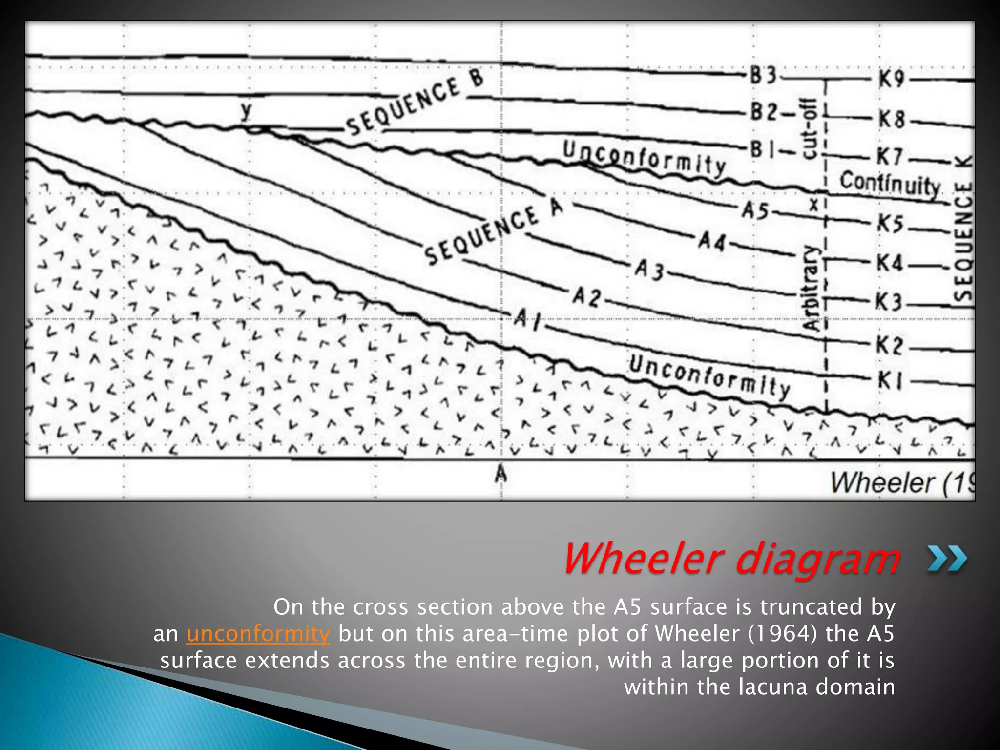
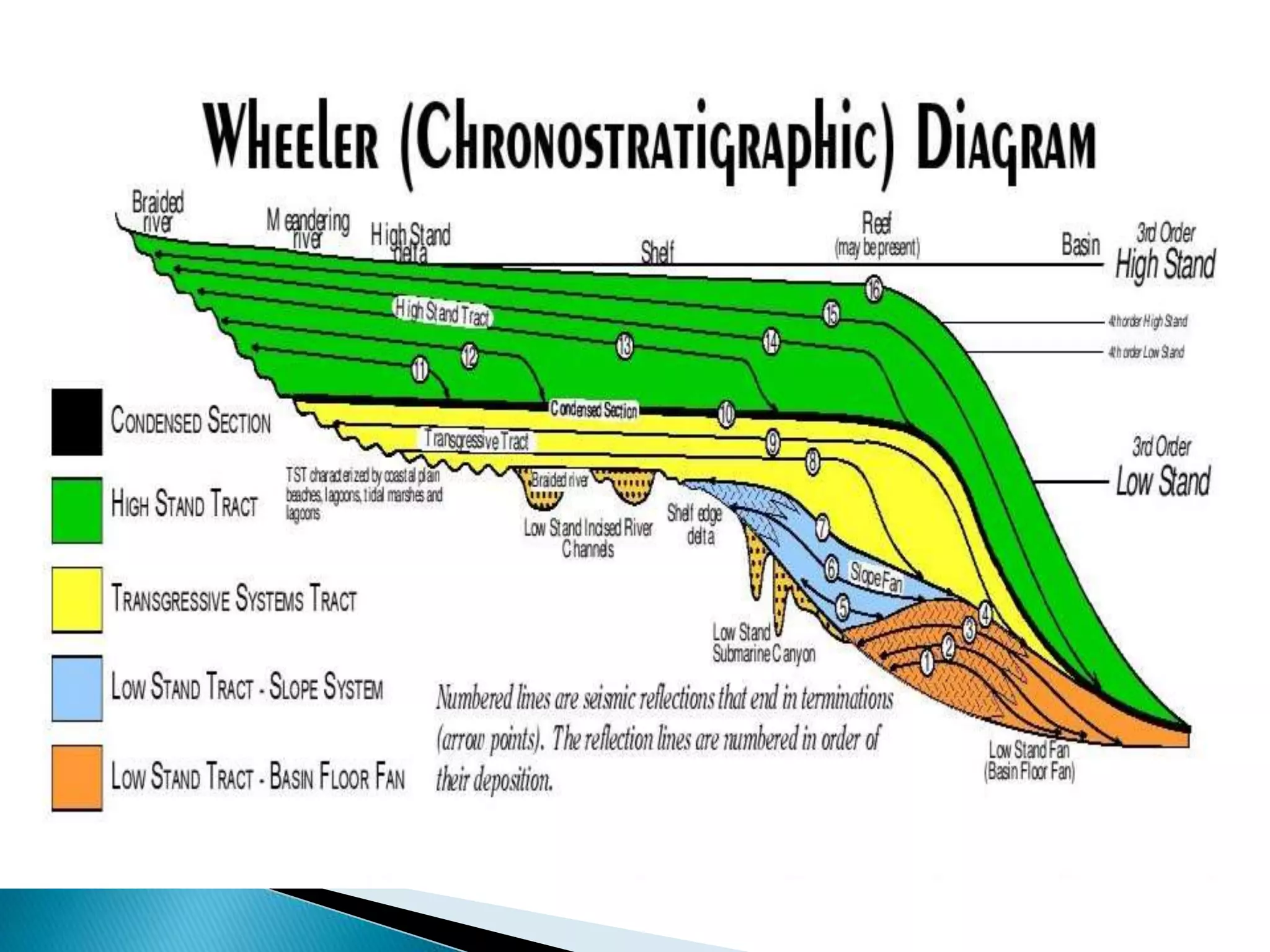
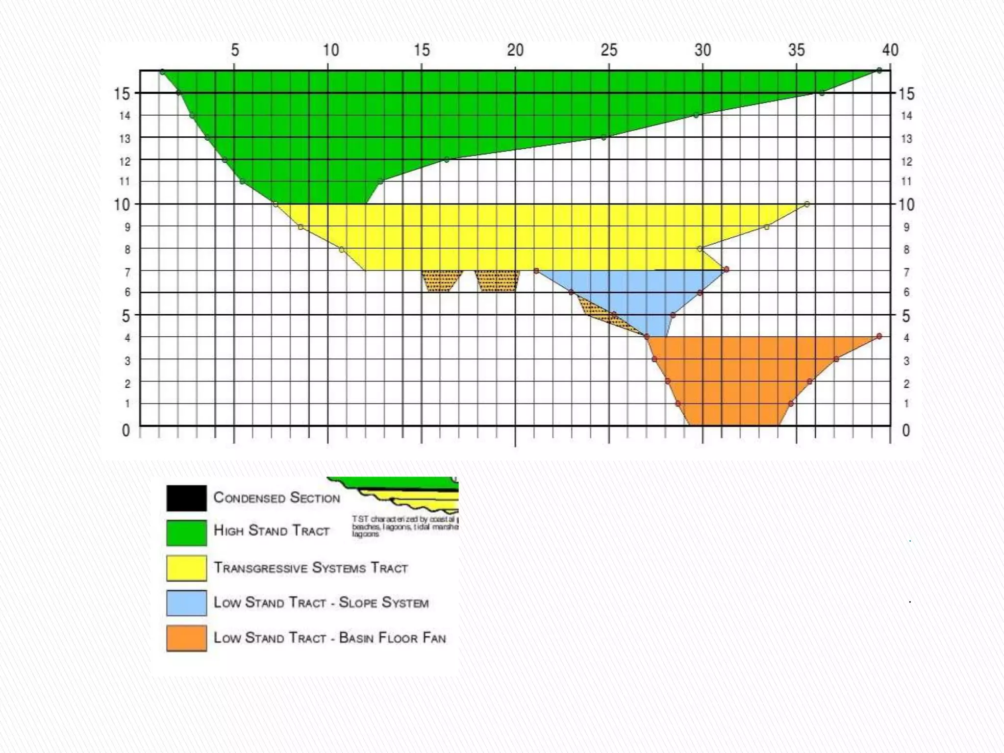
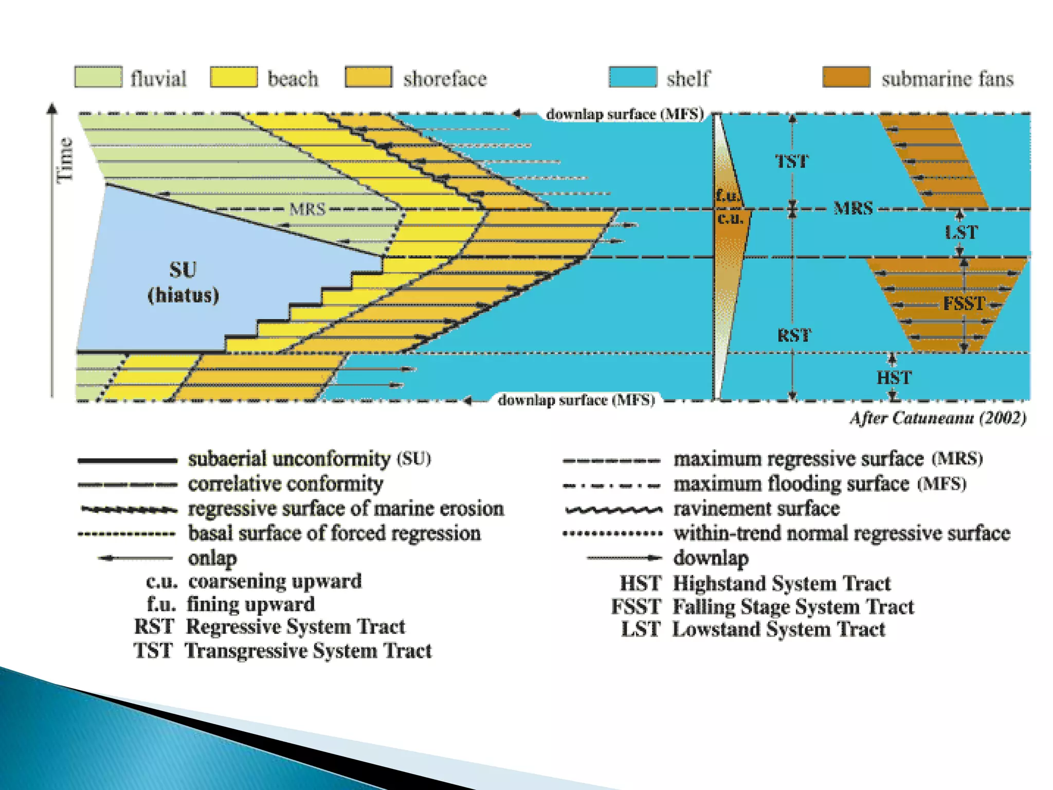
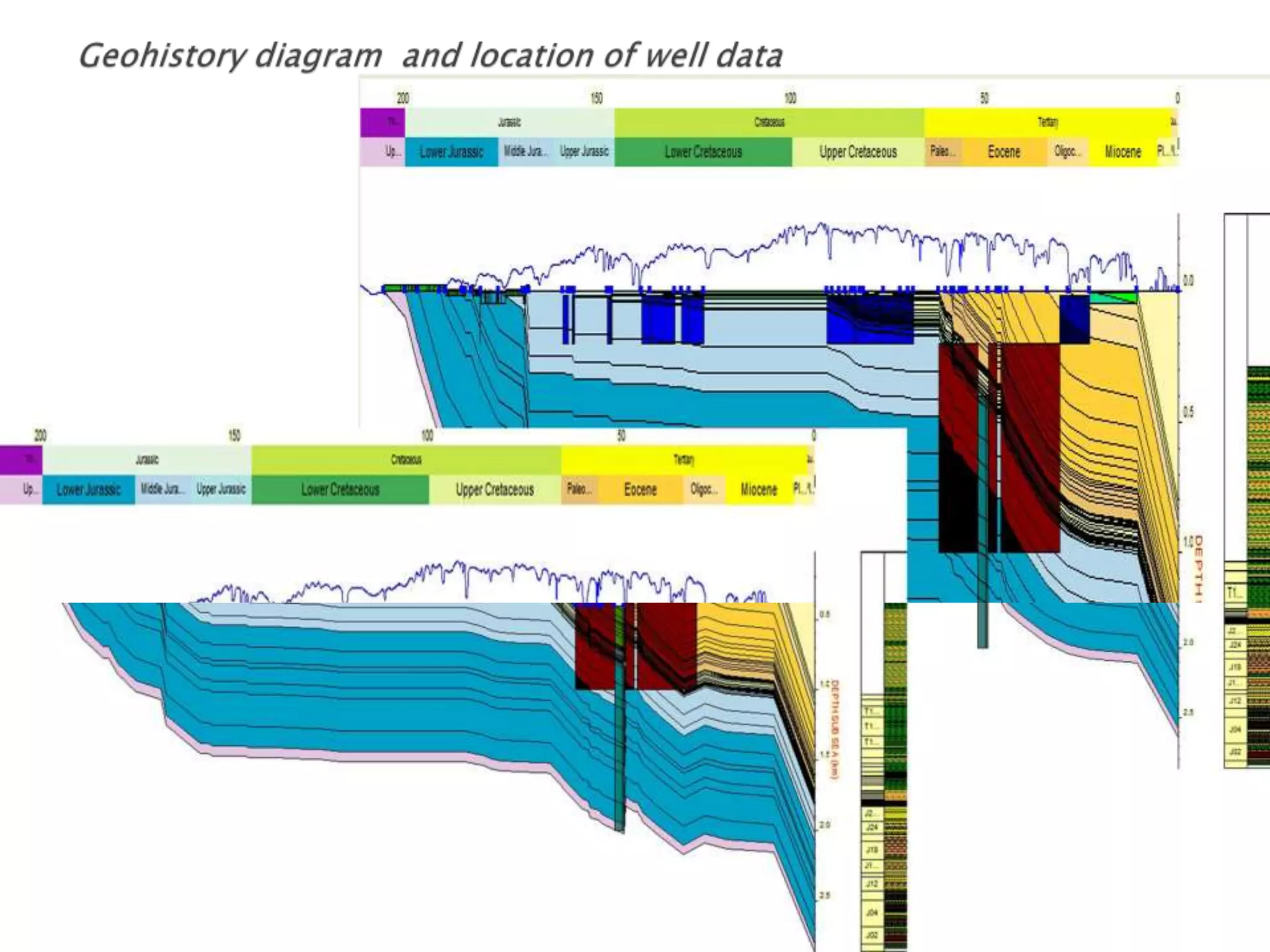
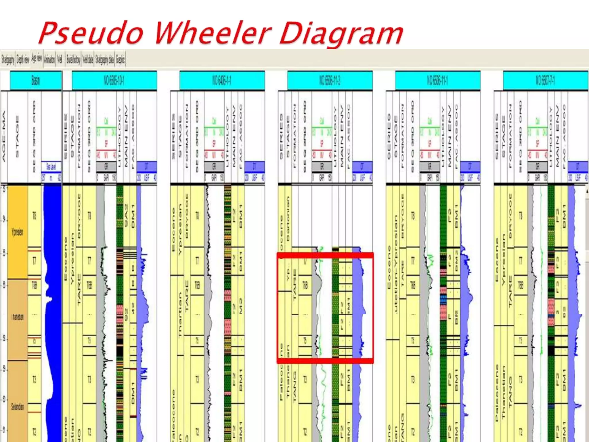
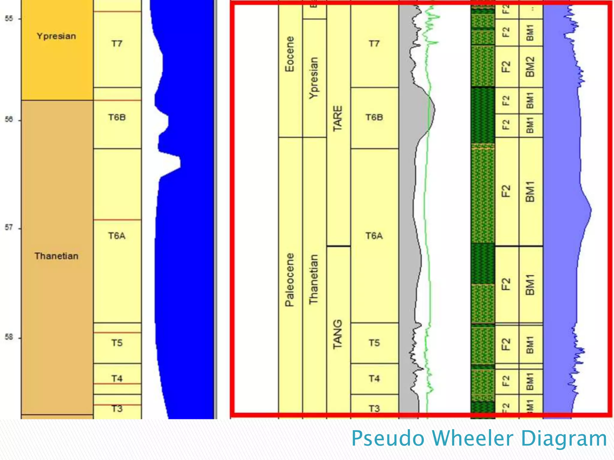
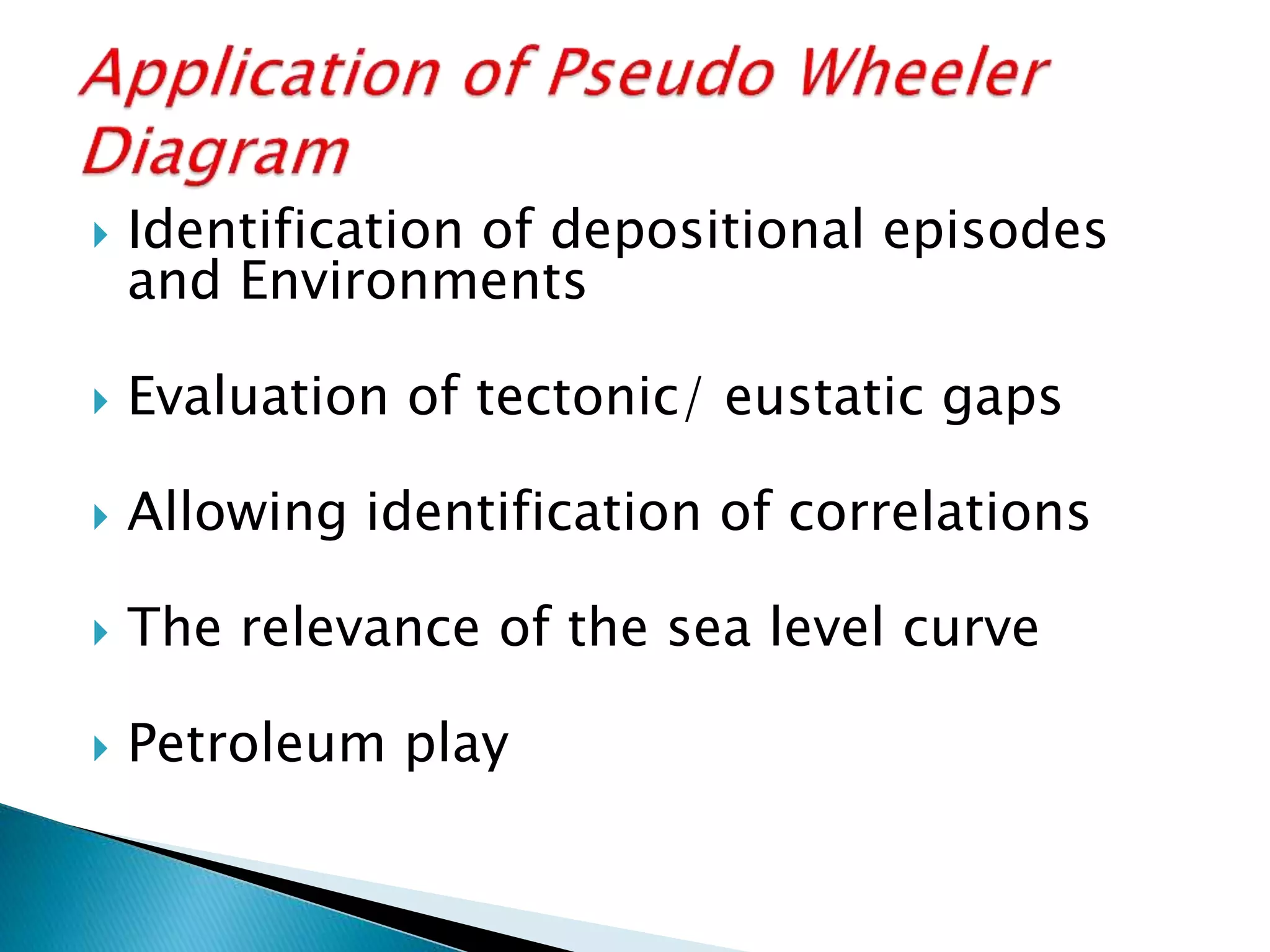
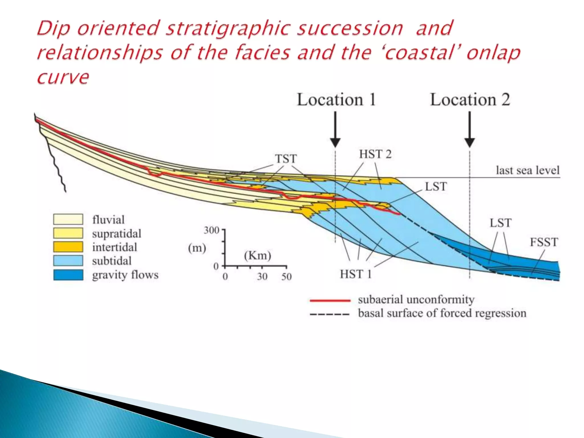
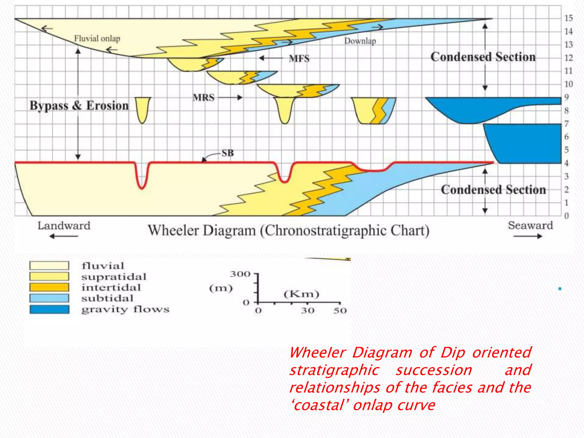
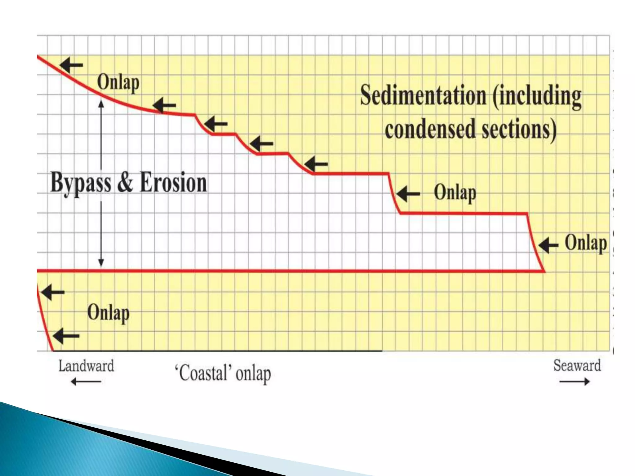
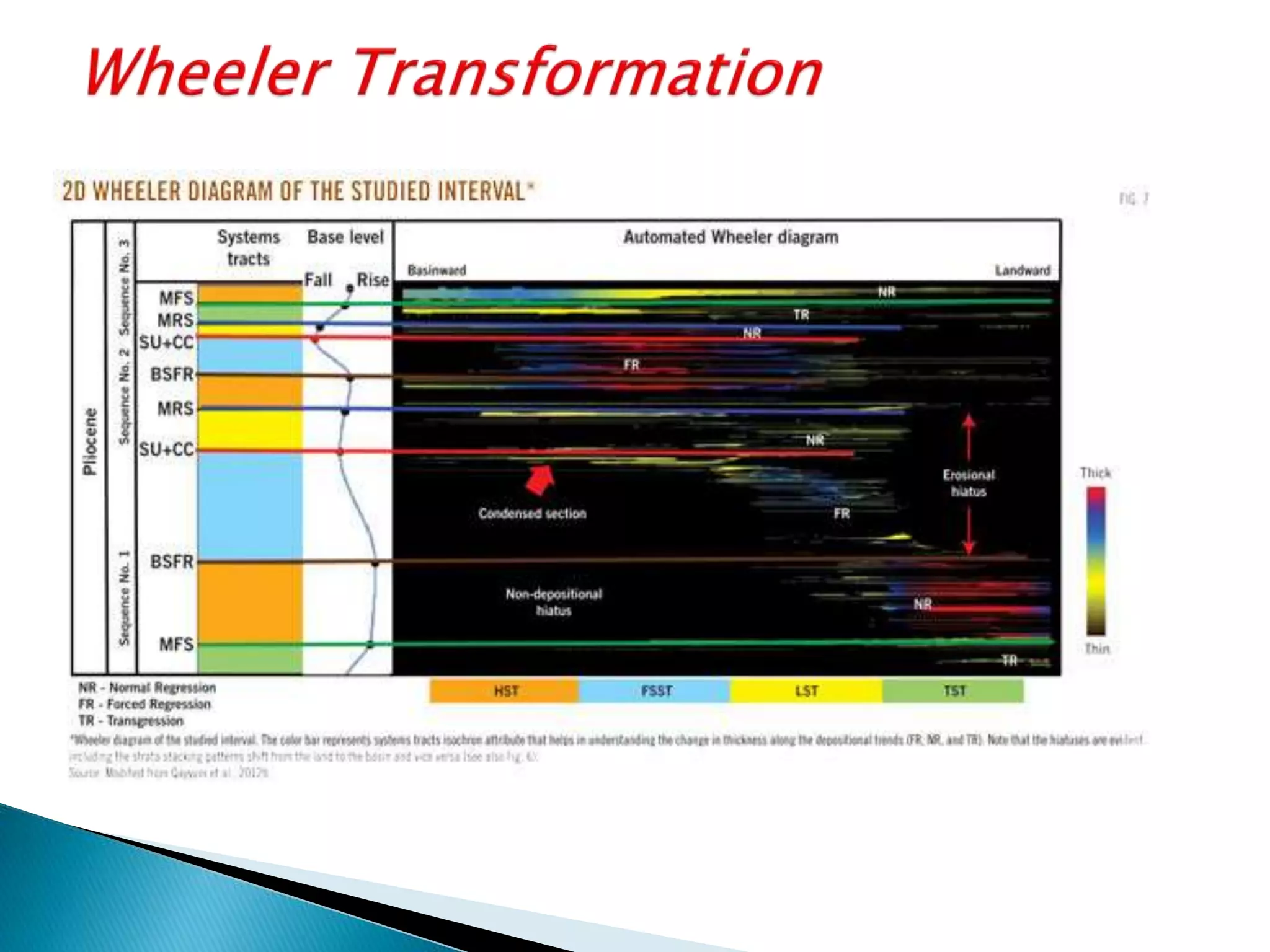
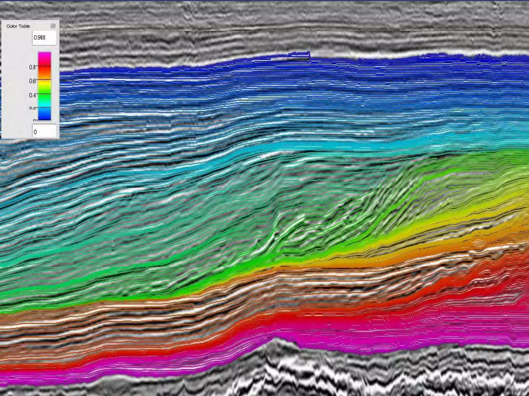
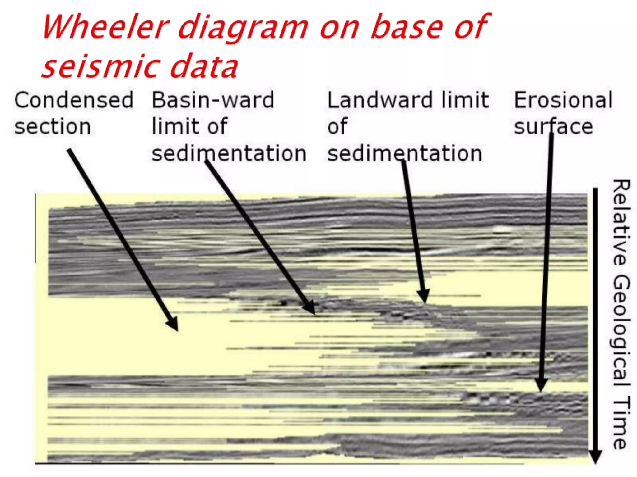
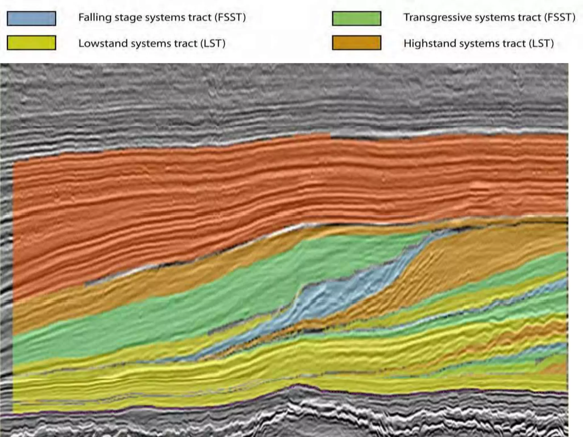
WHEELER DIAGRAM
&
ITS USES IN EXPLORATION
AND EXPLOITATION IN
HYDROCORBONS
Presented by:
Awais Ayub Awan
Muhammad Umar
Muhammad Sajid
Presented to:
Mr. Abdul Hannan
 Wheeler Diagram
 Harry Eugene Wheeler ( History to Wheeler
diagram)
 Integrated data of Wheeler Diagram
 Application of Wheeler diagram in
Exploration and hydrocarbon exploitation
 Wheeler Diagrams related to base level
changes, system tracts, stratigraphic
surfaces, Unconformity
 Wheeler diagram of a fluvial to shallow-
marine depositional sequence
(Dip oriented stratigraphic succession)
 Interpretation of Wheeler diagram of
a fluvial to shallow-marine
depositional sequence
 Wheeler diagram on the base of well
log data
 (Pseudo Wheeler diagram)
 Calibration through Pseudo wheeler
diagram
 workflow for interpretation of Pseudo
Wheeler Diagram
 wheeler diagram related to
interpretation of Coastal onlap curve
 Wheeler transformation ( seismic
based wheeler diagram
 Uses of Wheeler diagram
 Conclusion
 References
 A stratigraphic summary chart on which
geologic time is plotted as the vertical scale,
and distance across the area of interest as the
horizontal scale, and on which a variety of
stratigraphic information is brought together.
 Display both the horizontal distribution of the
contemporaneous component sedimentary
layers of a sequence but also the
significant hiatuses in sedimentation.
 Stratigraphic summary chart
 It’s a spatio-temporal diagram
 Consist of x-axis and y-axis
 On x-axis plot distance of stratigraphic area
of interest
 On y-axis plot Geologic age ( absolute and
relative) of stratigraphic section
On the cross section above the A5 surface is truncated by
an unconformity but on this area-time plot of Wheeler (1964) the A5
surface extends across the entire region, with a large portion of it is
within the lacuna domain
Wheeler diagram
 American Geologist and Stratigraphic
 (1907 – 26 January 1987)
 A professor of geology at the University of
Washington from 1948 until 1976
 Wheeler's work in the 1950 and 1960s was
pivotal in the later development of sequence
stratigraphy
 still used today, for example by Petroleum
industry
 His 1964 paper, Baselevel, Lithosphere
Surface, and Time-Stratigraphy evolved the
concept of base level
 To emphasize the continuous spatial and
temporal nature of stratigraphy, eventually
giving rise to wheeler diagram.
 The contemporaneous component
sedimentary layers
 Systems tracts of sequences in terms
of their relationship to
baselevel, hiatuses, timing and
geographic location.
Outcrops data
Core data
Well logs
Seismic data
 Base level change
 Interplay between base level change and
sedimentation
 Interpretation of sedimentary environment
 Stacking pattern (Progaradation &
retrogradation)
 System tracts
 Sequences Surfaces
 Unconformity
 Deposition
 Condensation
 Erosion
 Hiatus
 Hydrocarbon exploration
 Economic minerals
 Geologic time and thickness of formation
 Geographic distance of stratigraphic
succession
.
.
 Depositional patterns during a full
regressive-transgressive cycle
 Base level Change
 For the stratal stacking patterns of the four
systems tracts
 Their inferred timing relative to the base-
level curve
 Subaerial unconformity extends basinward
 Due to forced regression of the shoreline
 correlative conformity meets the basinward
termination of the subaerial unconformity
 Appearance of fluvial onlap depends on
topographic gradients
 Grading trends (fining- vs. coarsening-upward) are
temporally offset between shallow- and deep-
water systems
 Progradation of basin-floor fans continues
throughout the regressive stage
 onset of base-level rise marks a change from high-
density to low-density turbidity currents
 sand starts to be trapped
 aggrading fluvial to coastal systems during
lowstand normal regression
 stratal architecture breakdown of a sequence into
the four systems tracts
 A full cycle of base-level changes consists of a
succession of four distinct stages of shoreline
shifts
 (i.e., two normal regressions, one transgression
and one forced regression)
 Its logic in separating the products of deposition of
four stages in the evolution of a sequence
 Each stage of shoreline shift is associated with
different economic opportunities
i. Petroleum plays,
ii. Exploration strategies
iii. change markedly between the products of forced
regression and subsequent lowstand normal
regression.
 Correlative conformity marked the end of
regression and base level fall
 (1)Fluvial to shallow-marine depositional sequence
 (2) Wheeler diagram
 based on the Upper Cretaceous succession in
southern Utah,
 End of the estuary life time (end of transgression)
is accompanied by an abrupt shift in fluvial styles
upstream
 It recognize nonmarine portion of the maximum
flooding surface.
 Landward shift of facies through time
 Boundary between braided and meandering
stream facies
 Fining upward trend within the fluvial part
of each systems tract.
 Threshold of facies shift across the
maximum flooding surface
 Maximum flooding surface in fluvial successions
indicated by an abrupt increase in fluvial energy,
from meandering to overlying braided fluvial
systems
 End estuary life time triggers a rapid seaward shift
of the river mouth ( delta)
 Maximum flooding surface is indicated by a grain
size.
 Wheeler Diagram interpreted on the base of
Well log data
Calibration through a 'pseudo Wheeler'
diagram
 A review of depositional episodes
 Tectonic/ Eustatic gaps,
 Allowing identification of correlations
 The relevance of the sea level curve
 1. Lithology
 2. Sequence Stratigraphy
 3. Environments and Facies
 4. Lithostratigraphy
 5. Chronostratigraphy
Pseudo Wheeler Diagram
 Identification of depositional episodes
and Environments
 Evaluation of tectonic/ eustatic gaps
 Allowing identification of correlations
 The relevance of the sea level curve
 Petroleum play
.
Wheeler Diagram of Dip oriented
stratigraphic succession and
relationships of the facies and the
‘coastal’ onlap curve
 ‘Coastal’ onlap curve is use in the seismic and
sequence stratigraphy for the construction of
the global cycle chart.
 Composed mainly of a combination of fluvial
and marine onlap.
 ‘Coastal’ onlap indicates stages of
sea-level rise is misleading, and resulted in
the representation of sea-level fall as
instantaneous events.
 Wheeler transform is the seismic equivalent of the
geologic Wheeler diagram.
 Flatten the seismic data (or derived attributes)
along flattened chrono-stratigraphic horizons.
 The vertical axis in the Wheeler transformed
domain is relative geologic time (as opposed to
absolute geologic time)
 Wheeler transform can be performed in 2D and 3D
 Purpose;
To flatten the seismic data while honoring
hiatuses caused by non-deposition and
erosion.
 Work flow;
i. Select a pre-calculated chrono-stratigraphy
ii. Add a Wheeler scene and use the selected
chrono-stratigraphy to flatten the seismic
data (or attribute).
 Wheeler diagrams provide a useful tool for
hydrocarbon exploration when it used in
junction with sequence stratigraphic
principles.
 Reservoir risks can be significantly reduced
by using such charts
 It use with sequence stratigraphic
depositional models to identify potential
sand-prone facies.
 Interpretation of sedimentary environment
 Stacking pattern (Progaradation &
retrogradation)
 Unconformity
 Economic minerals
 Principle of Sequence stratigraphy by
Octuvian Catuneanu
 Sequence stratigraphy by Emry
 Web search
Google Books
Google Images
www.wikipedia.com
www.geology.com
www.scl.com
Strata terminology site
Wheeler Diagram and interpretation of wheeler diagram

Wheeler Diagram and interpretation of wheeler diagram

  • 2.
    WHEELER DIAGRAM & ITS USESIN EXPLORATION AND EXPLOITATION IN HYDROCORBONS
  • 3.
    Presented by: Awais AyubAwan Muhammad Umar Muhammad Sajid Presented to: Mr. Abdul Hannan
  • 4.
     Wheeler Diagram Harry Eugene Wheeler ( History to Wheeler diagram)  Integrated data of Wheeler Diagram  Application of Wheeler diagram in Exploration and hydrocarbon exploitation  Wheeler Diagrams related to base level changes, system tracts, stratigraphic surfaces, Unconformity  Wheeler diagram of a fluvial to shallow- marine depositional sequence (Dip oriented stratigraphic succession)
  • 5.
     Interpretation ofWheeler diagram of a fluvial to shallow-marine depositional sequence  Wheeler diagram on the base of well log data  (Pseudo Wheeler diagram)  Calibration through Pseudo wheeler diagram  workflow for interpretation of Pseudo Wheeler Diagram
  • 6.
     wheeler diagramrelated to interpretation of Coastal onlap curve  Wheeler transformation ( seismic based wheeler diagram  Uses of Wheeler diagram  Conclusion  References
  • 7.
     A stratigraphicsummary chart on which geologic time is plotted as the vertical scale, and distance across the area of interest as the horizontal scale, and on which a variety of stratigraphic information is brought together.  Display both the horizontal distribution of the contemporaneous component sedimentary layers of a sequence but also the significant hiatuses in sedimentation.
  • 8.
     Stratigraphic summarychart  It’s a spatio-temporal diagram  Consist of x-axis and y-axis  On x-axis plot distance of stratigraphic area of interest  On y-axis plot Geologic age ( absolute and relative) of stratigraphic section
  • 9.
    On the crosssection above the A5 surface is truncated by an unconformity but on this area-time plot of Wheeler (1964) the A5 surface extends across the entire region, with a large portion of it is within the lacuna domain Wheeler diagram
  • 10.
     American Geologistand Stratigraphic  (1907 – 26 January 1987)  A professor of geology at the University of Washington from 1948 until 1976  Wheeler's work in the 1950 and 1960s was pivotal in the later development of sequence stratigraphy  still used today, for example by Petroleum industry
  • 11.
     His 1964paper, Baselevel, Lithosphere Surface, and Time-Stratigraphy evolved the concept of base level  To emphasize the continuous spatial and temporal nature of stratigraphy, eventually giving rise to wheeler diagram.
  • 12.
     The contemporaneouscomponent sedimentary layers  Systems tracts of sequences in terms of their relationship to baselevel, hiatuses, timing and geographic location.
  • 13.
  • 14.
     Base levelchange  Interplay between base level change and sedimentation  Interpretation of sedimentary environment  Stacking pattern (Progaradation & retrogradation)  System tracts  Sequences Surfaces
  • 15.
     Unconformity  Deposition Condensation  Erosion  Hiatus  Hydrocarbon exploration  Economic minerals  Geologic time and thickness of formation  Geographic distance of stratigraphic succession
  • 17.
  • 19.
     Depositional patternsduring a full regressive-transgressive cycle  Base level Change  For the stratal stacking patterns of the four systems tracts  Their inferred timing relative to the base- level curve
  • 20.
     Subaerial unconformityextends basinward  Due to forced regression of the shoreline  correlative conformity meets the basinward termination of the subaerial unconformity  Appearance of fluvial onlap depends on topographic gradients
  • 21.
     Grading trends(fining- vs. coarsening-upward) are temporally offset between shallow- and deep- water systems  Progradation of basin-floor fans continues throughout the regressive stage  onset of base-level rise marks a change from high- density to low-density turbidity currents  sand starts to be trapped
  • 22.
     aggrading fluvialto coastal systems during lowstand normal regression  stratal architecture breakdown of a sequence into the four systems tracts  A full cycle of base-level changes consists of a succession of four distinct stages of shoreline shifts  (i.e., two normal regressions, one transgression and one forced regression)
  • 23.
     Its logicin separating the products of deposition of four stages in the evolution of a sequence  Each stage of shoreline shift is associated with different economic opportunities i. Petroleum plays, ii. Exploration strategies iii. change markedly between the products of forced regression and subsequent lowstand normal regression.  Correlative conformity marked the end of regression and base level fall
  • 25.
     (1)Fluvial toshallow-marine depositional sequence  (2) Wheeler diagram  based on the Upper Cretaceous succession in southern Utah,  End of the estuary life time (end of transgression) is accompanied by an abrupt shift in fluvial styles upstream  It recognize nonmarine portion of the maximum flooding surface.
  • 26.
     Landward shiftof facies through time  Boundary between braided and meandering stream facies  Fining upward trend within the fluvial part of each systems tract.  Threshold of facies shift across the maximum flooding surface
  • 27.
     Maximum floodingsurface in fluvial successions indicated by an abrupt increase in fluvial energy, from meandering to overlying braided fluvial systems  End estuary life time triggers a rapid seaward shift of the river mouth ( delta)  Maximum flooding surface is indicated by a grain size.
  • 28.
     Wheeler Diagraminterpreted on the base of Well log data Calibration through a 'pseudo Wheeler' diagram  A review of depositional episodes  Tectonic/ Eustatic gaps,  Allowing identification of correlations  The relevance of the sea level curve
  • 29.
     1. Lithology 2. Sequence Stratigraphy  3. Environments and Facies  4. Lithostratigraphy  5. Chronostratigraphy
  • 32.
  • 33.
     Identification ofdepositional episodes and Environments  Evaluation of tectonic/ eustatic gaps  Allowing identification of correlations  The relevance of the sea level curve  Petroleum play
  • 35.
    . Wheeler Diagram ofDip oriented stratigraphic succession and relationships of the facies and the ‘coastal’ onlap curve
  • 37.
     ‘Coastal’ onlapcurve is use in the seismic and sequence stratigraphy for the construction of the global cycle chart.  Composed mainly of a combination of fluvial and marine onlap.  ‘Coastal’ onlap indicates stages of sea-level rise is misleading, and resulted in the representation of sea-level fall as instantaneous events.
  • 38.
     Wheeler transformis the seismic equivalent of the geologic Wheeler diagram.  Flatten the seismic data (or derived attributes) along flattened chrono-stratigraphic horizons.  The vertical axis in the Wheeler transformed domain is relative geologic time (as opposed to absolute geologic time)  Wheeler transform can be performed in 2D and 3D
  • 39.
     Purpose; To flattenthe seismic data while honoring hiatuses caused by non-deposition and erosion.  Work flow; i. Select a pre-calculated chrono-stratigraphy ii. Add a Wheeler scene and use the selected chrono-stratigraphy to flatten the seismic data (or attribute).
  • 44.
     Wheeler diagramsprovide a useful tool for hydrocarbon exploration when it used in junction with sequence stratigraphic principles.  Reservoir risks can be significantly reduced by using such charts  It use with sequence stratigraphic depositional models to identify potential sand-prone facies.
  • 45.
     Interpretation ofsedimentary environment  Stacking pattern (Progaradation & retrogradation)  Unconformity  Economic minerals
  • 46.
     Principle ofSequence stratigraphy by Octuvian Catuneanu  Sequence stratigraphy by Emry  Web search Google Books Google Images www.wikipedia.com www.geology.com www.scl.com Strata terminology site