2. q = 0.65ag͑Ug − V͒2
ͫ2͑Ug − V͒a
g
ͬ−0.81
, ͑3͒
where a is the cross-sectional radius, g and g are the gas
density and kinematic viscosity, respectively.
Equation ͑1͒ is readily integrated, which yields
a2
V = a0
2
V0, ͑4͒
where subscript zero designates the cross-sectional radius
and longitudinal velocity values at the “initial” cross-section.
This expression allows one to exclude the cross-sectional
radius from the consideration, as is done below.
In thin liquid jets the normal stress in the cross-section
can be always presented as a difference between the normal
and radial deviatoric stresses, xx and yy, respectively, i.e.,
as2
xx=xx−yy. The deviatoric stresses should be related to
the flow kinematics via a rheological constitutive equation
͑RCE͒. For polymeric liquids experiencing strong uniaxial
stretching as, for example, in meltblowing, an appropriate
RCE is the viscoelastic upper-convected Maxwell model7
͑UCM͒, which is substantiated by direct statistical consider-
ation of macromolecular stretching and the corresponding
entropic elasticity.2
In the present case, the RCE of the Max-
well model reduces to the following axial and radial ͑lateral͒
projections:
V
dxx
dx
= 2
dV
dx
xx +
2
dV
dx
−
xx
, ͑5͒
V
dyy
dx
= −
dV
dx
yy −
dV
dx
−
yy
, ͑6͒
where and are the liquid viscosity and relaxation time,
respectively.
Combining Eqs. ͑2͒–͑6͒, we can transform them to the
following system of dimensionless equations
dV
dx
=
͓− E͑xx − yy͒/͑DeV
2
͒ + q͔
͓1 − E͑xx + 2yy + 3͒/V
2
͔
, ͑7͒
dxx
dx
=
1
V
ͩ2
dV
dx
xx + 2
dV
dx
−
xx
De
ͪ, ͑8͒
dyy
dx
=
1
V
ͩ−
dV
dx
yy −
dV
dx
−
yy
De
ͪ, ͑9͒
where
q = 0.65Rᐉ/V
1/2
͑Ug − V͒2
͓Re͑Ug − V͒/V
1/2
͔−0.81
. ͑10͒
The equations are rendered dimensionless by the following
scales: V0 for V and Ug, the distance between the “initial”
cross-section and deposition screen L for x, a0 for a, / for
xx and yy, and further on, L/V0 for time t. The primary
dimensionless groups involved in Eqs. ͑7͒–͑10͒ are given by
R =
g
, ᐉ =
L
a0
, Re =
2V0a0
g
, De =
V0
L
, ͑11͒
with Re and De being the Reynolds and Deborah numbers,
respectively; the secondary dimensionless groups are
E =
2R
Deᐉ Re M
, M =
g
. ͑12͒
In Eq. ͑12͒ g denotes gas viscosity.
The system of three ordinary differential Eqs. ͑7͒–͑9͒ is
subjected to the following dimensional conditions at the “ini-
tial” cross-section of the polymer jet:
x = 0:V = 1, xx = xx0, yy = 0. ͑13͒
The fact that all boundary conditions for Eqs. ͑7͒–͑9͒ can be
imposed at x=0 stems from the hyperbolicity of this system
of equations, which holds if the dimensional initial velocity
V0 is larger than the dimensional speed of the “elastic
sound”2,8,9
͑xx/͒1/2
. Accounting for Eq. ͑13͒, the latter cor-
responds to the following dimensionless condition:
1 Ͼ Exx0. ͑14͒
This means that even though polymeric liquids can develop
rather significant longitudinal deviatoric stresses in flow in-
side the die and carry a significant part of it as xx0 to the
“initial” cross-section,10
the convective effects in the poly-
meric jet are initially stronger than propagation of the “elas-
tic sound.” Therefore, the information in such a jet is con-
vected downstream, even though the “elastic sound” can
propagate not only down- but also upstream ͑i.e., against the
flow, but swept by it͒. In such cases all boundary conditions
are imposed at the beginning of the polymer jet as in Eq.
͑13͒.
The system of Eqs. ͑7͒–͑9͒ subjected to the conditions
͑13͒ was solved numerically using the Kutta–Merson
method.
The solution of Eqs. ͑7͒–͑9͒ for the unperturbed jet is
illustrated in Figs. 1–3 for the following values of the param-
eters: M=0.001, R=0.00122, ᐉ=83000, De=0.01, and Re
=40, the dimensionless velocity of the gas flow assumed to
be constant in the present case is Ug=Ug͑0͒=10, xx0=104
,
H0=0.01, and the dimensionless perturbation frequency ⍀
=L/V0=1500. These values of the dimensionless groups
correspond to plausible values of the physical parameters
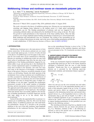
FIG. 1. The unperturbed distributions of the longitudinal velocity ͑solid
line͒ and cross-sectional radius ͑dashed line͒ along polymer jet stretched by
high speed gas jet.
034913-2 Yarin, Sinha-Ray, and Pourdeyhimi J. Appl. Phys. 108, 034913 ͑2010͒
Downloaded 23 Mar 2011 to 131.193.154.219. Redistribution subject to AIP license or copyright; see http://jap.aip.org/about/rights_and_permissions
3. partially taken from Ref. 11: a0=3ϫ10−3
cm, L=250 cm,
g=1.22ϫ10−3
g/cm3
, g=0.15 cm2
/s, V0=103
cm/s, the
dimensional Ug͑0͒=104
cm/s, =0.25ϫ10−2
s, and =6
ϫ103
Hz.
Figure 1 depicts the unperturbed longitudinal velocity
V͑x͒ and radius a͑x͒ distributions, and Figs. 2͑a͒ and 2͑b͒—
the unperturbed distributions of the longitudinal and lateral
deviatoric stresses, xx͑x͒ and yy͑x͒, respectively. It is seen
that the polymer jet is gradually accelerated by the aerody-
namic drag imposed by the gas stream, and simultaneously
thins ͑Fig. 1͒. The longitudinal deviatoric stress xx, which is
rather high at the die exit due to the prior strong stretching in
the die channel, decreases along the jet because the elonga-
tion rate due to the gas flow there is insufficiently high to
overcome the viscoelastic relaxation ͓the so-called, weak
flow; cf. Fig. 2͑a͔͒. Comparison of Figs. 2͑a͒ and 2͑b͒ shows
that the lateral deviatoric stress yy is negligibly small com-
pared to the lateral one, xx, as expected in the uniaxial elon-
gational flows.
III. SMALL PERTURBATIONS OF POLYMERIC
VISCOELASTIC LIQUID JET IN PARALLEL HIGH-
SPEED GAS FLOW
Bending perturbations of polymer jets stretched by high
speed gas jet will be studied using the quasi-one-dimensional
equations of the dynamics of free liquid jets.2
In the moment-
less approximation ͑neglecting the bending stiffness͒ and as-
suming small bending perturbations ͑linearizing͒, one can
reduce Eqs. ͑4.19͒ on p. 49 in Ref. 2 to the normal projection
of the momentum balance equation in the following dimen-
sional form:
ץ2
H
ץt2 + 2V
ץ2
H
ץx ץ t
+ ͫV
2
+
g͑Ug − V͒2
− xx
ͬץ2
H
ץx2 = 0.
͑15͒
Rendering this equation dimensionless using the scales listed
above in Sec. II, the following dimensionless equation is
obtained:
ץ2
H
ץt2 + 2V
ץ2
H
ץx ץ t
+ ͓V
2
+ R͑Ug − V͒2
− Exx͔
ץ2
H
ץx2 = 0,
͑16͒
where L is also used as a scale for the perturbation amplitude
⌯. Equations ͑15͒ and ͑16͒ are kindred to Eq. ͑6͒ in Ref. 1
for the bending perturbations of a solid flexible threadline.
It is emphasized that in the linear approximation, pertur-
bations of the longitudinal flow do not affect small bending
perturbations, i.e., the latter are completely uncoupled from
the former ones, since the coupling could happen only via
nonlinear terms. Therefore, in Eq. ͑16͒ the factors multiply-
ing the derivatives in the second and third terms on the left
depend on the unperturbed distributions of V͑x͒ and
xx͑x͒=xx͑x͒−yy͑x͒, which are found from Eqs. ͑7͒–͑9͒.
The general solution of Eq. ͑16͒ can be found using the
characteristics
FIG. 2. The unperturbed distributions of the longitudinal ͑a͒, and lateral ͑b͒ deviatoric stresses ͑xx and yy, respectively͒ along polymer jet stretched by high
speed gas jet.
FIG. 3. Distribution of K͑x͒.
034913-3 Yarin, Sinha-Ray, and Pourdeyhimi J. Appl. Phys. 108, 034913 ͑2010͒
Downloaded 23 Mar 2011 to 131.193.154.219. Redistribution subject to AIP license or copyright; see http://jap.aip.org/about/rights_and_permissions
4. dx
dt
= V Ϯ ͓Exx − R͑Ug − V͒2
͔1/2
. ͑17͒
Equation ͑16͒ is hyperbolic if Exx−R͑Ug−V͒2
Ͼ0 and the
characteristics are real, and elliptic if Exx−R͑Ug−V͒2
Ͻ0
and the characteristics are complex. This means that if at x
=0, the inequality Exx0ϾR͓Ug͑0͒−1͔2
holds, the initial part
of the jet is “hyperbolic.” Given Eq. ͑14͒, the conditions that
the initial part of the jet is “hyperbolic” in both unperturbed
and perturbed states are
1 Ͼ Exx0 Ͼ R͓Ug͑0͒ − 1͔2
. ͑18͒
The transition cross-section x=xء is found from the follow-
ing equation:
K͑x͒ = Exx͑x͒ − R͓Ug͑x͒ − V͑x͔͒2
= 0. ͑19͒
The general solution of Eq. ͑16͒ is given by
H͑x,t͒ = ⌽ͫ͵0
x
dx
V + ͱExx − R͑Ug − V͒2
− tͬ
+ Fͫ͵0
x
dx
V − ͱExx − R͑Ug − V͒2
− tͬ ͑20͒
where ⌽͑·͒ and F͑·͒ are arbitrary functions.
Assume that the inequalities ͑18͒ hold. Then, the initial
part of the polymeric jet 0ՅxՅxء is “hyperbolic,” whereas
the following part xءՅxՅ1 “elliptic.”
Here again, as in the case of the threadline,1
we apply
the conditions for the perturbation wave at the “initial” cross-
section of the polymer jet in the following form:
H͉x=0 = H0 exp͑it͒, ץ H/ץx͉x=0 = 0 ͑21͒
which corresponds to the overall effect of the turbulent pul-
sations being combined there.
Then, we can find the functions ⌽͑·͒ and F͑·͒ and re-
duce Eq. ͑20͒ to the following solution for the “hyperbolic”
part at 0ՅxՅxء
H͑x,t͒ =
H0
1 − ␦
exp͑it͕͒− ␦ exp͓− iI1͑x͔͒
+ exp͓− iI2͑x͔͖͒, ͑22͒
where the two real functions I1͑x͒ and I2͑x͒ are given by
I1͑x͒ = ͵0
x
dx
V͑x͒ + ͱExx͑x͒ − R͓Ug͑x͒ − V͑x͔͒2
, ͑23͒
I2͑x͒ = ͵0
x
dx
V͑x͒ − ͱExx͑x͒ − R͓Ug͑x͒ − V͑x͔͒2
, ͑24͒
and
␦ = ͯdI2/dx
dI1/dx
ͯx=0
. ͑25͒
The corresponding solution for the “elliptic” ͑in regards to
bending perturbations͒ part of the polymer jet at xءՅxՅ1 is
also obtained from the general solution ͑20͒. After it is
matched to the “hyperbolic” solution at the transition point
x=xء, it reads
H͑x,t͒ =
H0
1 − ␦
exp͕i͓t − J1͑x͔͖͒
ϫ ͕− ␦ exp͓− iI1͑xء͔͒exp͓− J2͑x͔͒
+ exp͓− iI2͑xء͔͒exp͓J2͑x͔͖͒. ͑26͒
In Eq. ͑26͒ the two additional real functions J1͑x͒ and J2͑x͒
are defined as
J1͑x͒ = ͵xء
x
V͑x͒
V
2
͑x͒ + R͓Ug͑x͒ − V͑x͔͒2
− Exx͑x͒
dx,
͑27͒
J2͑x͒ = ͵xء
x ͱR͓Ug͑x͒ − V͑x͔͒2
− Exx͑x͒
V
2
͑x͒ + R͓Ug͑x͒ − V͑x͔͒2
− Exx͑x͒
dx.
͑28͒
It is emphasized that the dimensional gas stream velocity at
the outer boundary of the boundary layer near the liquid jet
surface, Ug͑x͒, can be evaluated using the theory of the axi-
symmetric turbulent gas jets12,13
as
Ug͑x͒ = Ug͑0͒
2.4d0
x + 2.4d0
, ͑29͒
where d0Ϸ2a0 is the diameter of the coaxial gas jet nozzle,
and 2.4d0 is the polar distance of the jet.
The corresponding dimensionless expression becomes
Ug͑x͒ = Ug͑0͒
4.8/ᐉ
x + 4.8/ᐉ
, ͑30͒
where Ug͑x͒ and Ug͑0͒ are rendered dimensionless by V0.
Figure 3 depicts the function K͑x͒ of Eq. ͑19͒, which is
obtained from the solution for the unperturbed straight jet in
Sec. II. It is seen that K͑x͒=0 at x=xء=0.146. This means
that at 0ՅxՅ0.146 bending perturbations are “hyperbolic,”
whereas at 0.146ՅxՅ1 they are “elliptic.” Two predicted
snapshots of the bending jet configurations corresponding to
two different time moments are shown in Fig. 4. It is seen
FIG. 4. Two snapshots ͑one shown by solid line, another one by the dashed
one͒ of the predicted traveling wave of the bending perturbations of polymer
jet enhanced by the distributed aerodynamic lift force.
034913-4 Yarin, Sinha-Ray, and Pourdeyhimi J. Appl. Phys. 108, 034913 ͑2010͒
Downloaded 23 Mar 2011 to 131.193.154.219. Redistribution subject to AIP license or copyright; see http://jap.aip.org/about/rights_and_permissions
5. that in the “hyperbolic” part described by Eq. ͑22͒ the trav-
eling perturbation wave has the amplitude of the order of
⌯0. After the transition to the “elliptic” part, the amplitude
of the traveling perturbation wave described by Eq. ͑26͒
even decreases, but after the bottleneck seen in Fig. 4 at
about x=0.35, the perturbation amplitude rapidly increases,
as is expected for an elliptic problem solved as an initial-
value problem. That is the area where the perturbed jet will
be drastically stretched and thinned. An accurate description
of such thinning can be achieved only in the framework of a
fully nonlinear description in the following section.
The pattern of the perturbation waves predicted for melt-
blowing in Fig. 4 is rather peculiar. It shows that the initial
part of the jet attached to the die can be almost straight, since
it is stabilized by sufficiently large longitudinal stresses gen-
erated in the die and still not fully vanished there. On the
other hand, when relaxation of the longitudinal stresses sig-
nificantly reduces their level, bending perturbations grow
and begin to release the stored energy delivered by the initial
perturbations ͑turbulent pulsations͒ and are also enhanced by
the distributed lift force. A renewed significant liquid stretch-
ing is expected because of strong bending, which will be also
accompanied by drastic thinning of polymer jet. This behav-
ior is quite similar to the patterns characteristic of electro-
spun polymer jets. In the latter case the bending force related
to the Coulombic repulsion is formally similar to the distrib-
uted aerodynamic lift force here ͑both are proportional to the
local curvature of the jet axis͒.5
The presence of significant
longitudinal viscoelastic stresses in the initial part of electro-
spun jets stabilizes them and they stay almost straight. Later
on, the stresses fade due to viscoelastic relaxation and strong
bending begins.4–6,10
Correspondingly, meltblown jets can
stay initially almost straight due to stabilization by high lon-
gitudinal stress. Only after it fades due to the dominant re-
laxation, a vigorous bending leading to jet elongation and
thinning begins.
IV. NONLINEAR BEHAVIOR: LARGE-AMPLITUDE
BENDING PERTURBATIONS IN THE ISOTHERMAL
CASE
In the quasi-one-dimensional theory of liquid jets two
types of approaches to describing jet bending ͑with and with-
out accounting for the bending stiffness͒ are available.2
In
the momentless approximation bending stiffness of very thin
liquid jets is neglected compared to the other internal forces
affecting bending, since it depends on the cross-sectional jet
radius as a4
, while the other forces as a2
͑which is much
larger as a tends to zero͒.2
In the present section we adopt the
momentless approximation and neglect the shearing force in
the jet cross-section and the whole moment-of-momentum
equation determining it. As a result, the quasi-one-
dimensional equations of the jet dynamics reduce to the au-
tonomous continuity and momentum balance equations in
the following form ͓Eqs. ͑4.18͒ on p. 48 in Ref. 2͔
ץf
ץt
+
ץfW
ץs
= 0, ͑31͒
ץfV
ץt
+
ץfWV
ץs
=
1
ץP
ץs
+ fg +
qtotal. ͑32͒
In Eqs. ͑31͒ and ͑32͒ t is time, s is an arbitrary parameter
͑coordinate͒ reckoned along the jet axis, f͑s,t͒=a2
is the
cross-sectional area ͓the cross-section is assumed to stay cir-
cular even in bending jets-a valid approximation according
to Ref. 2; a͑s,t͒ denotes its radius͔, W is the liquid velocity
along the jet relative to a cross-section with a certain value of
s, the stretching factor =͉ץR/ץs͉, where R͑s,t͒ is the posi-
tion vector of the jet axis, V͑s,t͒ is the absolute velocity in
the jet, is liquid density, P͑s,t͒ is the magnitude of the
longitudinal internal force of viscoelastic origin in the jet
cross-section, is the unit tangent vector of the jet axis, g is
gravity acceleration, and qtotal is the overall aerodynamic
force imposed on unit jet length by the surrounding gas.
Boldfaced characters here and hereinafter denote vectors.
Let s be a Lagrangian parameter of liquid elements in the
jet ͑e.g., their initial Cartesian coordinate along the blowing
direction͒. Then, W=0, since the particles keep their La-
grangian coordinate unchanged, and Eq. ͑31͒ is integrated to
yield
a2
= 0a0
2
, ͑33͒
where subscript zero denotes the initial values.
Consider for example two-dimensional bending pertur-
bations of the jet ͑the fully three-dimensional bending can be
considered similarly along the same lines2
͒. Then, account-
ing for Eq. ͑33͒, the two projections of Eq. ͑32͒ on the di-
rections of the local tangent and unit normal n to the jet
axis read
ץV
ץt
= Vnͩ1
ץVn
ץs
+ kVͪ+
1
f
ץP
ץs
+ g +
qtotal,
f
, ͑34͒
ץVn
ץt
= − Vͩ1
ץVn
ץs
+ kVͪ+
Pk
f
+ gn +
qtotal,n
f
, ͑35͒
where k is the local curvature of the jet axis and subscripts
and n denote vector projections on the local tangent and
normal to the jet axis.
In the case of planar bending, the position vector of the
jet axis is described as
R = i͑s,t͒ + jH͑s,t͒, ͑36͒
with i and j being the unit vectors of the directions of blow-
ing and the direction normal to it, respectively, while the
geometric parameters and k are given by
= ͑,s
2
+ ⌯,s
2
͒1/2
, ͑37͒
k =
⌯,ss,s − ,ss⌯,s
͑,s
2
+ ⌯,s
2
͒3/2
. ͑38͒
The total aerodynamic force is comprised from the distrib-
uted longitudinal lift force2,3
͓a nonlinear analog of the lin-
earized lift force incorporated in Eq. ͑15͔͒, the distributed
drag force associate with gas flow across the jet2,3
and the
pulling drag force similar to that of Eq. ͑3͒. Therefore,
034913-5 Yarin, Sinha-Ray, and Pourdeyhimi J. Appl. Phys. 108, 034913 ͑2010͒
Downloaded 23 Mar 2011 to 131.193.154.219. Redistribution subject to AIP license or copyright; see http://jap.aip.org/about/rights_and_permissions
6. qtotal = nqtotal,n + qtotal, = − gUg
2
nͫf
,s
2
͑⌯,ss,s − ,ss⌯,s͒
͑,s
2
+ ⌯,s
2
͒5/2
+ a
͑⌯,s/,s͒2
sign͑⌯,s/,s͒
1 + ͑⌯,s/,s͒2 ͬ+ ag͑Ug
− V͒2
0.65ͫ2a͑Ug − V͒
g
ͬ−0.81
, ͑39͒
where Ug is the magnitude of the absolute local blowing
velocity of gas, and corresponds to its projection on the
local direction of the polymer jet axis.
In addition, in Eqs. ͑34͒ and ͑35͒ the projections of the
gravity acceleration g and gn are equal to g=g and gn
=gn with g being its magnitude and n the local projection
of the unit normal to the jet axis onto the direction of blow-
ing.
The longitudinal internal force of viscoelastic origin in
the jet cross-section2
P=f͑−nn͒ where and nn are the
longitudinal and normal deviatoric stresses in the jet cross-
section. As usual, in the case of strong stretching ͑cf. for
example, Sec. II͒, ӷnn and the latter can be neglected.
Then, P=f where the constitutive equation for is pro-
vided by the viscoelastic7
UCM in the form
ץ
ץt
= 2
1
ץ
ץt
+ 2
1
ץ
ץt
−
. ͑40͒
Equations ͑33͒–͑35͒ and ͑37͒–͑40͒ which describe jet dy-
namics are supplemented by the following kinematic equa-
tions which describe the axis shape:
ץ
ץt
= Vn − Vn, ͑41͒
ץ⌯
ץt
= Vn − Vn ͑42͒
The projections of the unit vectors associated with the poly-
mer jet axis and n on the directions of the unit vectors i
and j associated with the blowing direction and normal to it
͑ and ⌯͒ are given by the following expressions:
= n = ͓1 + ͑⌯,s/,s͒2
͔−1/2
, ͑43͒
n = − = − ͑⌯,s/,s͓͒1 + ͑⌯,s/,s͒2
͔−1/2
. ͑44͒
According to the theory of the axisymmetric turbulent gas
jets,12,13
the gas flow field is given by the following expres-
sion:
Ug͑,⌯͒ = Ug0͑,⌯͒, ͑45͒
where Ug0 is the gas velocity of the nozzle exit and the
dimensionless function ͑,H͒ is given by
͑,H͒ =
4.8/ᐉ
͑ + 4.8/ᐉ͒
1
͑1 + 2
/8͒2, = ͑,⌯͒
=
H
0.05͑ + 4.8/ᐉ͒
. ͑46͒
In Eq. ͑46͒ and ⌯ are rendered dimensionless by L, the
distance between the “initial” cross-section and deposition
screen, and ᐉ is given by Eq. ͑11͒.
Neglecting secondary terms, the governing equations of
the problem ͑34͒, ͑35͒, and ͑40͒–͑42͒ in the isothermal case
can be reduced to the following dimensionless form:
ץ2
ץt2 =
2
Re
⌽
ץ2
ץs2 +
1
Fr2 + Jᐉ
qtotal,
f
, ͑47͒
ץ2
⌯
ץt2 = ͫ
Re
− J2
͑,⌯͒ͬ1
2
ץ2
⌯
ץs2 +
n
Fr2
− Jᐉ
2
͑,⌯͒
a
͑⌯,s/,s͒2
sign͑⌯,s/,s͒
1 + ͑⌯,s/,s͒2 , ͑48͒
where ⌽=͑+1/De͒−2
satisfies the following equation:
ץ⌽
ץt
= −
De2 , ͑49͒
In Eq. ͑47͒
qtotal, = a͓͑,⌯͒ − V͔2
0.65͕Rea a͓͑,⌯͒
− V͔͖−0.81
. ͑50͒
The following scales have been used: L/Ug0 for t; L for s,
and ⌯; L−1
for k; Ug0/L for and ⌽; Ug0 for Ug, V and
Vn; a0 for a ͑and a0
2
for f͒; gUg0
2
a0 for qtotal,; / for the
kinematic turbulent eddy viscosity t ͑used below; cf. Ref.
1͒. As a result, the following dimensionless groups arise in
addition to ᐉ=L/a0:
Re =
LUg0
, J =
g
, Fr = ͩUg0
2
gL
ͪ1/2
,
Rea =
2a0Ug0
g
, De =
Ug0
L
, ͑51͒
where Re and Rea are the corresponding Reynolds numbers,
Fr is the Froude number, and De is the Deborah number.
It is emphasized that the governing quasi-one-
dimensional equations in the general case of the three-
dimensional ͑nonplanar͒ meltblowing were derived from the
vectorial Eqs. ͑31͒ and ͑32͒ similarly to two-dimensional
planar ones, Eqs. ͑47͒ and ͑48͒. They are not present here for
the sake of brevity.
Based on the results in,1
we assume that turbulent pul-
sations in the gas jet impose lateral perturbations at the ori-
gin of the polymer melt jet at s=sorigin. Therefore, similarly
to Eq. ͑11͒ and using the results of,1
the boundary conditions
for Eqs. ͑47͒ and ͑48͒ are given by the following dimension-
less expressions:
͉s=sorigin
= 0, ⌯͉s=sorigin
= ⌯0⍀ exp͑i⍀t͒, ͑52͒
where
H0⍀ = ͑0.06 Re1/2
/ᐉ͒1/2
/0
1/4
, ⍀ =
L
Ug0
, ͑53͒
with 0 being the dimensionless longitudinal stress in the
jet inherited from the nozzle.
034913-6 Yarin, Sinha-Ray, and Pourdeyhimi J. Appl. Phys. 108, 034913 ͑2010͒
Downloaded 23 Mar 2011 to 131.193.154.219. Redistribution subject to AIP license or copyright; see http://jap.aip.org/about/rights_and_permissions
7. On the other hand, at the free end s=sfree and the jet is
assumed to be fully unloaded, i.e.,
,s͉sfree end
= 1, ⌯,s͉sfree end
= 0 ͑54͒
The initial condition for Eq. ͑49͒ at the moment when a
liquid element leaves the nozzle and enters the jet reads
⌽͉t=tbirth
= ͑0 + 1/De͒/0
2
. ͑55͒
V. NONLINEAR BEHAVIOR: NONISOTHERMAL
CASE
In the nonisothermal case polymer melt is surrounded by
hot gas jet, which is blowing into the space filled with cold
gas. As a result, the gas jet is cooled and the encased poly-
mer melt jet is cooled either and solidifies. Following Ref. 2,
we assume that the viscosity and relaxation time of polymer
melt vary with melt temperature T according to the following
expressions:
= 0 expͫU
Rg
ͩ1
T
−
1
T0
ͪͬ, = 0
T0
T
expͫU
Rg
ͩ1
T
−
1
T0
ͪͬ, ͑56͒
where T0 is the melt and gas jet temperature at the origin, 0
and 0 are the corresponding values of the viscosity and re-
laxation time, U is the activation energy of viscous flow, and
Rg is the absolute gas constant.
The thermal balance equation for a jet element reads
ץ
ץt
͑cTf͒ = − h͑T − Tg͒2a, ͑57͒
where c is the specific heat, h is the heat transfer coefficient,
and Tg the local gas temperature.
Using Eq. ͑33͒ and rendering temperatures T and Tg di-
mensionless by T0, rearrange Eq. ͑57͒ to the following di-
mensionless form:
ץT
ץt
= − 2Nuᐉ
JC
Rea Prg
0
͑T − Tg͒, ͑58͒
where Prg is the molecular Prandtl number for gas, C
=cpg/c is the ratio of the specific heat at constant pressure for
gas to the specific heat for polymer melt, and the Nusselt
number Nu=͑h2a/kg͒, with kg being the molecular thermal
conductivity of gas, is given by the following expression:5
Nu = 0.495 Rea
1/3
Prg
1/2
. ͑59͒
Substituting Eqs. ͑56͒ into Eq. ͑40͒ and using Eq. ͑58͒, we
obtain the following dimensionless RCE replacing Eq. ͑49͒:
ץ⌽
ץt
= −
2NuᐉJC
Rea PrgDe00
͑T − Tg͒
− T expͫ− UAͩ1
T
− 1ͪͬ
De02 , ͑60͒
with ⌽=͑+T/De0͒/2
and the following two additional
dimensionless groups involved:
De0 =
0Ugo
L
, UA =
U
RgT0
. ͑61͒
Using the theory of the axisymmetric turbulent gas jets,13
the
temperature field in the gas jet is given by the following
expression:
Tg͑,⌯͒ = Tgϱ +
͑Prt + 1/2͒
0.05ͱ6
͑1 − Tgϱ͒
ᐉ
1
͑ + 4.8/ᐉ͒
ϫ
1
͑1 + 2
/8͒2Prt
, ͑62͒
where Tgϱ is the surrounding cold gas temperature far from
the polymer jet rendered dimensionless by T0, the turbulent
Prandtl number Prt=0.75, and ͑,⌯͒ is given by the second
Eq. ͑46͒.
It is emphasized that the other governing equations of
the problem, e.g., Eqs. ͑46͒–͑48͒ and ͑50͒ do not change in
the nonisothermal case.
VI. RESULTS AND DISCUSSION
The governing Eq. ͑48͒ is a hyperbolic wave equation
for ͑s,t͒, which corresponds to propagation of the elastic
compression-expansion waves along the jet ͑the “elastic
sound”͒. The second governing Eq. ͑49͒ responsible for the
propagation of the bending perturbations ⌯͑s,t͒ is a hyper-
bolic wave equation if jet is stretched significantly, i.e.,
͓/Re−J2
͑,⌯͔͒Ͼ0. If the longitudinal jet stretching
would fade due to the elastic relaxation and the distributed
lift force J2
͑,⌯͒ would become dominating, Eq. ͑49͒
changes type and becomes elliptic, since the factor ͓/Re
−J2
͑,H͔͒ becomes negative. This behavior has already
been mentioned in the linearized version of this problem in
Sec. III, which has drastic consequences on perturbation
growth.
The following parameter values partially corresponding
to those of Ref. 11 were used in the numerical calculations:
a0=0.2 cm, L=200 cm, Ug0=230 m/s, =1 g/cm3
,
=102
g/͑cm s͒, and g=1.22ϫ10−3
g/cm3
. Therefore, the
corresponding values of Re, J, and ᐉ were about Re
=46 000, J=10−3
, and ᐉ=103
. The effect of gravity was ex-
cluded, which corresponds to Fr=ϱ. The initial longitudinal
elastic stress was taken as 0=10 and 0=1. The relaxation
time was taken about =0.1 s, which corresponds to De
=10. In addition, it was taken C=0.25 and ⍀=0.3 ͑the latter
corresponds to =35 Hz; cf. Ref. 1͒. Also, Tgϱ=0.5 and
UA=10. The value of Rea for air ͑g=0.15 cm2
/s͒ is about
46 000. However, at such value of Rea the pulling aerody-
namic drag described by Eq. ͑50͒ is insufficient to initiate
meltblowing. This might be related to the fact that the em-
pirical Eq. ͑50͒ was established in Ref. 14 in the experiments
with threadlines pulled through stagnant air. However, drag
imposed by blowing air may be dramatically increased due
to the turbulent eddy viscosity ͑absent in the experiments14
͒.
To account for that fact, the factor 0.65 in Eq. ͑50͒ was
replaced by 1265. Then, the aerodynamic drag as per Eq.
͑50͒ became quite sufficient to initiate meltblowing.
The implicit numerical scheme of the generalized
Crank–Nicolson type with the central difference special dis-
034913-7 Yarin, Sinha-Ray, and Pourdeyhimi J. Appl. Phys. 108, 034913 ͑2010͒
Downloaded 23 Mar 2011 to 131.193.154.219. Redistribution subject to AIP license or copyright; see http://jap.aip.org/about/rights_and_permissions
8. cretisation at three time levels from Ref. 15 ͑p. 444͒ was
implemented to solve Eqs. ͑47͒ and ͑48͒ numerically.
The mean axisymmetric velocity and temperature fields
in the central domain close to the jet origin calculated using
Eqs. ͑45͒, ͑46͒, and ͑62͒ are presented in Fig. 5. Since the
turbulent Prandtl number Prt is less than 1 ͑Prt=0.75͒, the
temperature profile in the gas jet is wider than the velocity
profile.
The predicted configurations of the jet axis in the iso-
thermal planar blowing process are depicted in Fig. 6. It is
seen that the polymer jet is pulled and strongly stretched by
the coflowing gas jet. The polymer jet also experiences lat-
eral perturbations due to turbulent eddies. These bending per-
turbations are significantly enhanced by the distributed aero-
dynamic lift force acting on the curved polymer jet. They
also propagate along the polymer jet as elastic waves, and
are additionally swept by local aerodynamic drag force act-
ing on the jet elements. The configurations of the polymer jet
can become rather complicated and self-intersecting in a
while ͓Fig. 6͑b͔͒, which is possible for a “phantom” jet but
forbidden to a real material one. Still, the evolution similar to
that in Fig. 6͑b͒ points at possible self-intersection in melt-
blowing, even in the case of a single jet considered here.
If one follows individual material Lagrangian elements
of the polymer jet, as we do in our calculations, their distri-
bution along the jet allows visualization of a nonuniform jet
stretching. Indeed, these material elements are visualized by
symbols on the jet axis in Fig. 7. The larger is the distance
along the jet between two neighboring symbols, the larger is
the local stretching of viscoelastic polymer melt in the cor-
responding jet section. Figure 7 clearly shows that initially
jet stretching is quite significant and growing in time ͑from
snapshot to snapshot in Fig. 7͒, however, it can deteriorate
further on due to the elastic recoil characteristic of viscoelas-
tic polymer melts, as well as a decreasing stretching by the
gas jet, which weakens down the flow.
Comparison of Figs. 7͑a͒ and 7͑b͒ allows us to visualize
the effect of cooling and solidification of the polymer jet. In
particular, it is seen that the growth of the bending perturba-
tions of the jet is arrested similarly to the electrospun jets
FIG. 5. ͑Color online͒ Axisymmetric velocity ͑left͒ and temperature ͑right͒ fields in the gas jet.
FIG. 6. Isothermal planar blowing. ͑a͒ Three snapshots of the axis configu-
ration of polymer jet at the dimensionless time t=15, 35, and 50 ͑the cor-
responding dimensional times are 0.13 s, 0.3 s, and 0.43 s, respectively͒. ͑b͒
The later snapshot of the polymer jet axis corresponding to the dimension-
less time t=75 ͑the corresponding dimensional time is 0.65 s͒.
034913-8 Yarin, Sinha-Ray, and Pourdeyhimi J. Appl. Phys. 108, 034913 ͑2010͒
Downloaded 23 Mar 2011 to 131.193.154.219. Redistribution subject to AIP license or copyright; see http://jap.aip.org/about/rights_and_permissions
9. described in Ref. 5. However, the jet does not become
straight but continues to sustain traveling bending perturba-
tions similarly to the flexible solid threadlines studied in the
first paper in this series.1
The predictions for the isothermal three-dimensional
blowing are shown in Fig. 8. In this case the configuration of
the jet axis is described using the following three projections
=͑s͒, H=H͑s͒, and Z=Z͑s͒ instead of the two, =͑s͒ and
H=H͑s͒, used in the planar case. The tendency for self-
intersection of the polymer jet is clearly seen in the three-
dimensional case as well.
VII. CONCLUSION
The linear and nonlinear theory of meltblowing devel-
oped in this work explains the physical mechanisms respon-
sible for jet configurations, and in particular the role of the
turbulent pulsations in gas jet, of the aerodynamic lift and
drag forces, as well of the longitudinal viscoelastic stress in
the polymer jet. The theory produces a plausible pattern of
the evolution of the jet in time and allows modeling of not
only planar but also three-dimensional jets. The current ver-
sion of the theory deals with a single polymer jet. The further
development will proceed toward calculations of multiple
jets and their interaction and even merging with each other-
the processes responsible for such defects of meltblown
products as roping. Self-intersection of polymer jets visual-
ized by the present results can lead to jet rupture in the case
of violent blowing which results in the so-called fly ͑small
jet segments contaminating the surrounding atmosphere͒.
The mechanism of fly formation will also be elucidated by
future development of the current model. Formation of the
so-called shots resulting from capillary breakup of polymer
jets at too high surrounding temperatures will also be tar-
geted after inclusion of capillarity in the model similarly to
Ref. 2. A comprehensive model of meltblowing requires
simulation of polymer flow in die nosepiece, which will be
aimed in the future model development. The last but not least
goal is in the prediction of the internal structure in the fibers
comprising nonwovens resulting from meltblowing. This in-
formation can be elucidated relating the predicted longitudi-
nal stresses “frozen” in the jet at the deposition screen to
such characteristic features as crystallininty and ultimately
strength.
Finally, we believe that this framework can be used to
establish the role of polymer-process interactions on the so-
called formation.
ACKNOWLEDGMENTS
The current work is supported by the Nonwovens Coop-
erative Research Center ͑NCRC͒.
1
S. Sinha-Ray, A. L. Yarin, and B. Pourdeyhimi, J. Appl. Phys. 108,
034912 ͑2010͒.
2
A. L. Yarin, Free Liquid Jets and Films: Hydrodynamics and Rheology
͑Longman, Harlow and Wiley, New York, 1993͒.
3
V. M. Entov and A. L. Yarin, J. Fluid Mech. 140, 91 ͑1984͒.
4
D. H. Reneker, A. L. Yarin, H. Fong, and S. Koombhongse, J. Appl. Phys.
87, 4531 ͑2000͒.
5
A. L. Yarin, S. Koombhongse, and D. H. Reneker, J. Appl. Phys. 89, 3018
͑2001͒.
6
D. H. Reneker, A. L. Yarin, E. Zussman, and H. Xu, Adv. Appl. Mech. 41,
FIG. 7. ͑a͒ Three snapshots of the polymer jet axis in the isothermal planar
blowing at the dimensionless time t=15, 35, and 50 ͑the corresponding
dimensional times are 0.13 s, 0.3 s, and 0.43 s, respectively͒ with the sym-
bols denoting the material elements of the jet. ͑b͒ Same in the nonisothermal
planar blowing.
FIG. 8. ͑Color online͒ Three snapshots of the polymer jet axis in the iso-
thermal three-dimensional blowing at the dimensional time moments t=15,
30, and 45 ͑the corresponding dimensional times are 0.13 s, 0.26 s, and 0.39
s, respectively͒.
034913-9 Yarin, Sinha-Ray, and Pourdeyhimi J. Appl. Phys. 108, 034913 ͑2010͒
Downloaded 23 Mar 2011 to 131.193.154.219. Redistribution subject to AIP license or copyright; see http://jap.aip.org/about/rights_and_permissions
10. 43 ͑2007͒.
7
G. Astarita and G. Marrucci, Principles of Non-Newtonian Fluid Mechan-
ics ͑McGraw-Hill, London, 1974͒.
8
V. M. Entov and K. S. Kestenboim, Fluid Dyn. 22, 677 ͑1987͒.
9
D. D. Joseph, Fluid Dynamics of Viscoelastic Liquids ͑Springer, Berlin,
1990͒.
10
T. Han, A. L. Yarin, and D. H. Reneker, Polymer 49, 1651 ͑2008͒.
11
N. Marheineke and R. Wegener, SIAM J. Appl. Math. 68, 1 ͑2007͒.
12
G. N. Abramovich, The Theory of Turbulent Jets ͑MIT, Boston, 1963͒.
13
A. L. Yarin, in Springer Handbook of Experimental Fluid Mechanics,
edited by C. Tropea, A. L. Yarin, and J. Foss ͑Springer, Berlin, 2007͒, pp.
57–82.
14
High-Speed Fiber Spinning, edited by A. Ziabicki and H. Kawai ͑Wiley,
New York, 1985͒.
15
R. M. M. Mattheij, S. W. Rienstra, and J. H. M. ten Thije Boonkkamp,
Partial Differential Equations ͑SIAM, Philadelphia, 2005͒.
034913-10 Yarin, Sinha-Ray, and Pourdeyhimi J. Appl. Phys. 108, 034913 ͑2010͒
Downloaded 23 Mar 2011 to 131.193.154.219. Redistribution subject to AIP license or copyright; see http://jap.aip.org/about/rights_and_permissions