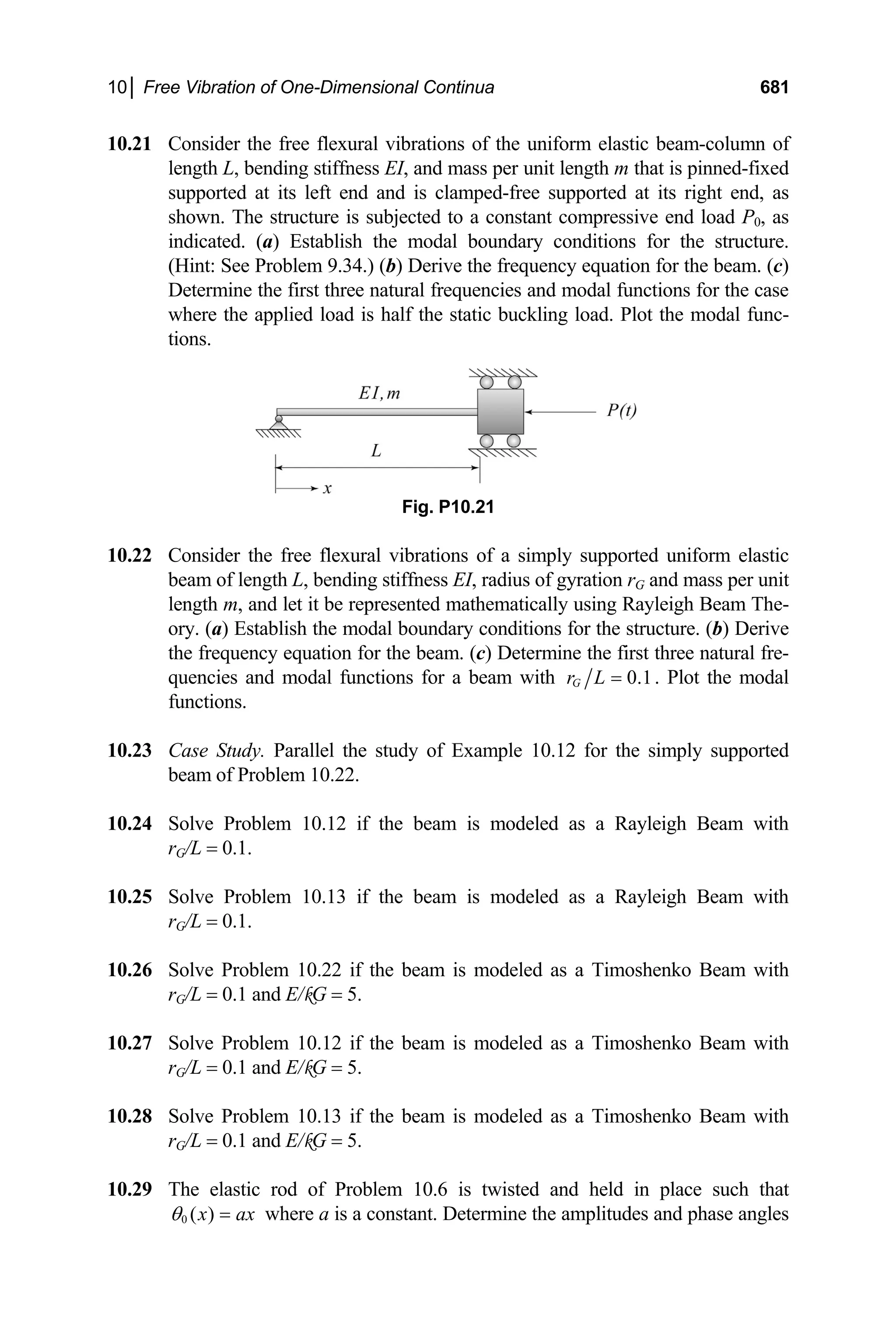
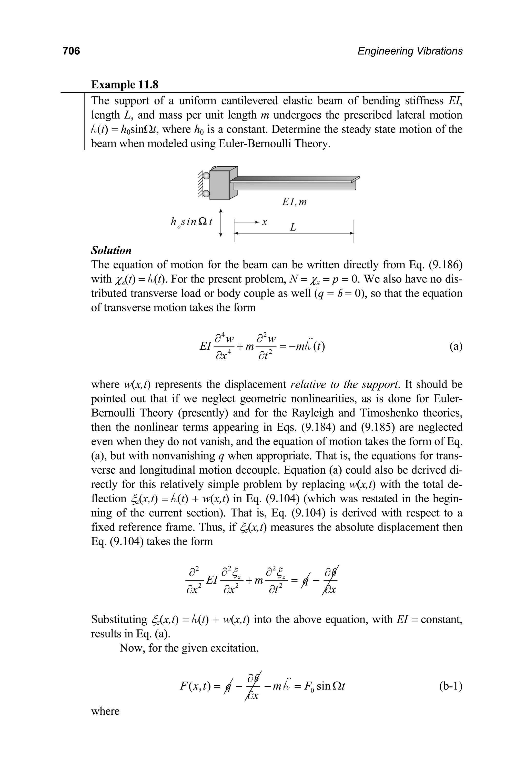
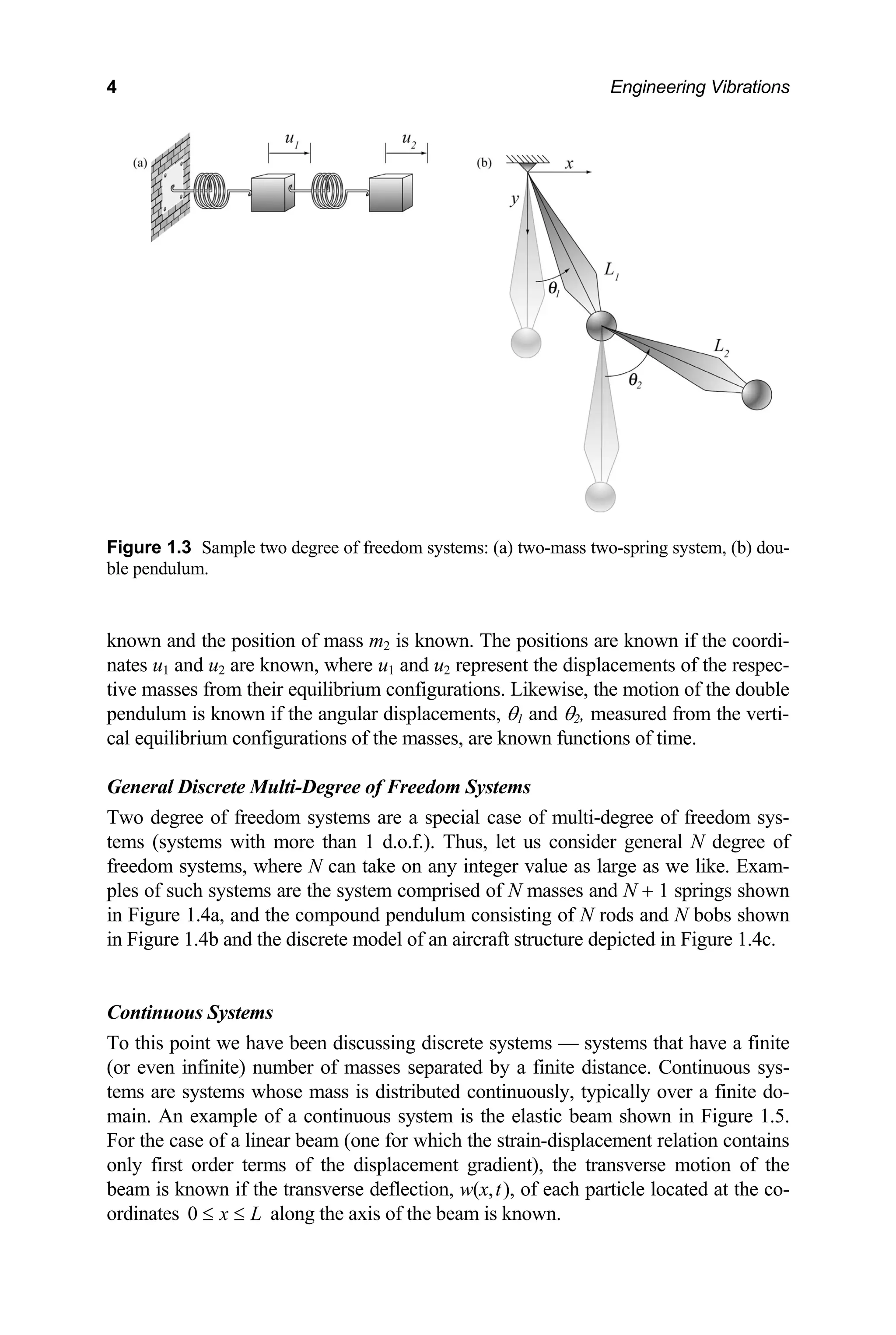
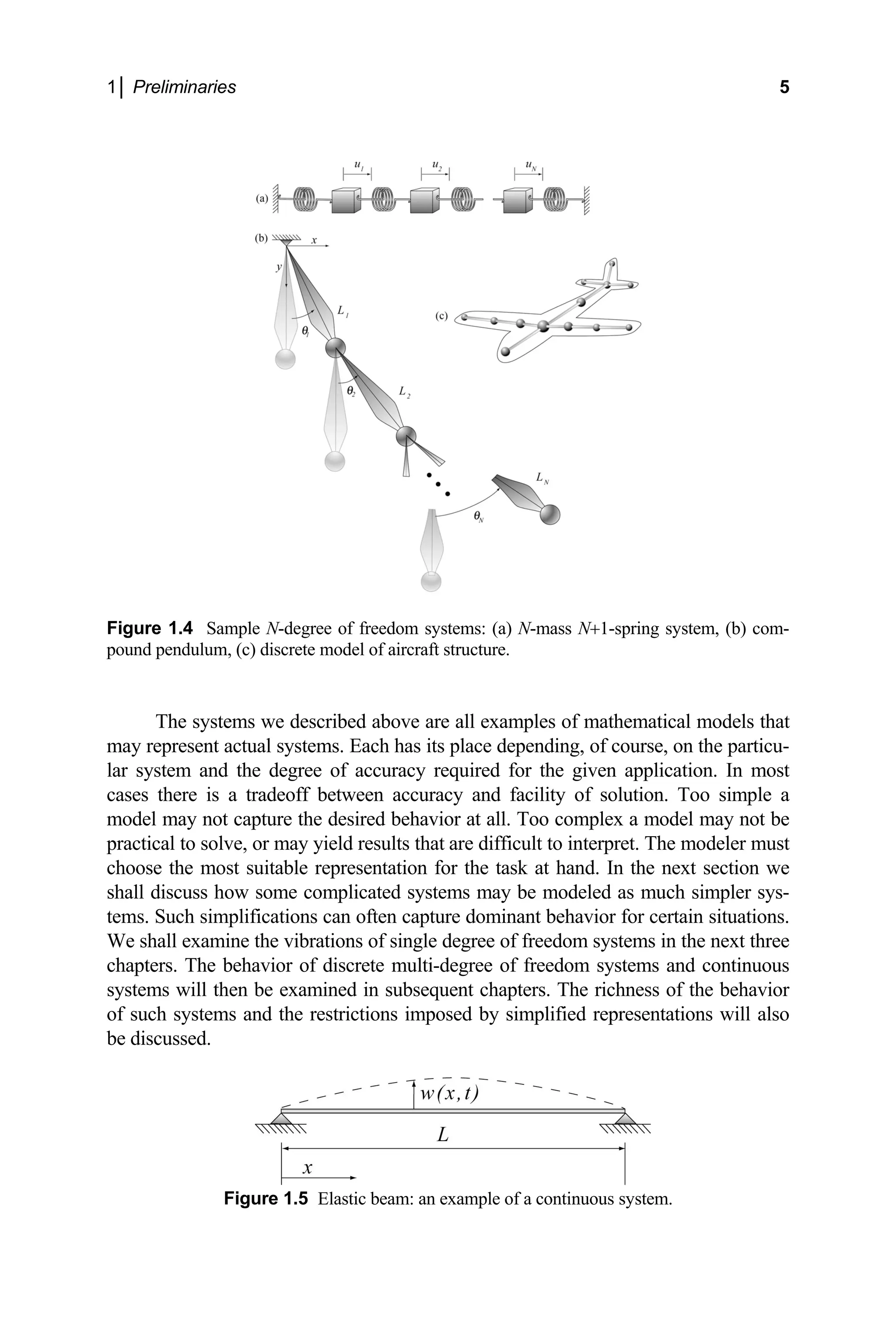
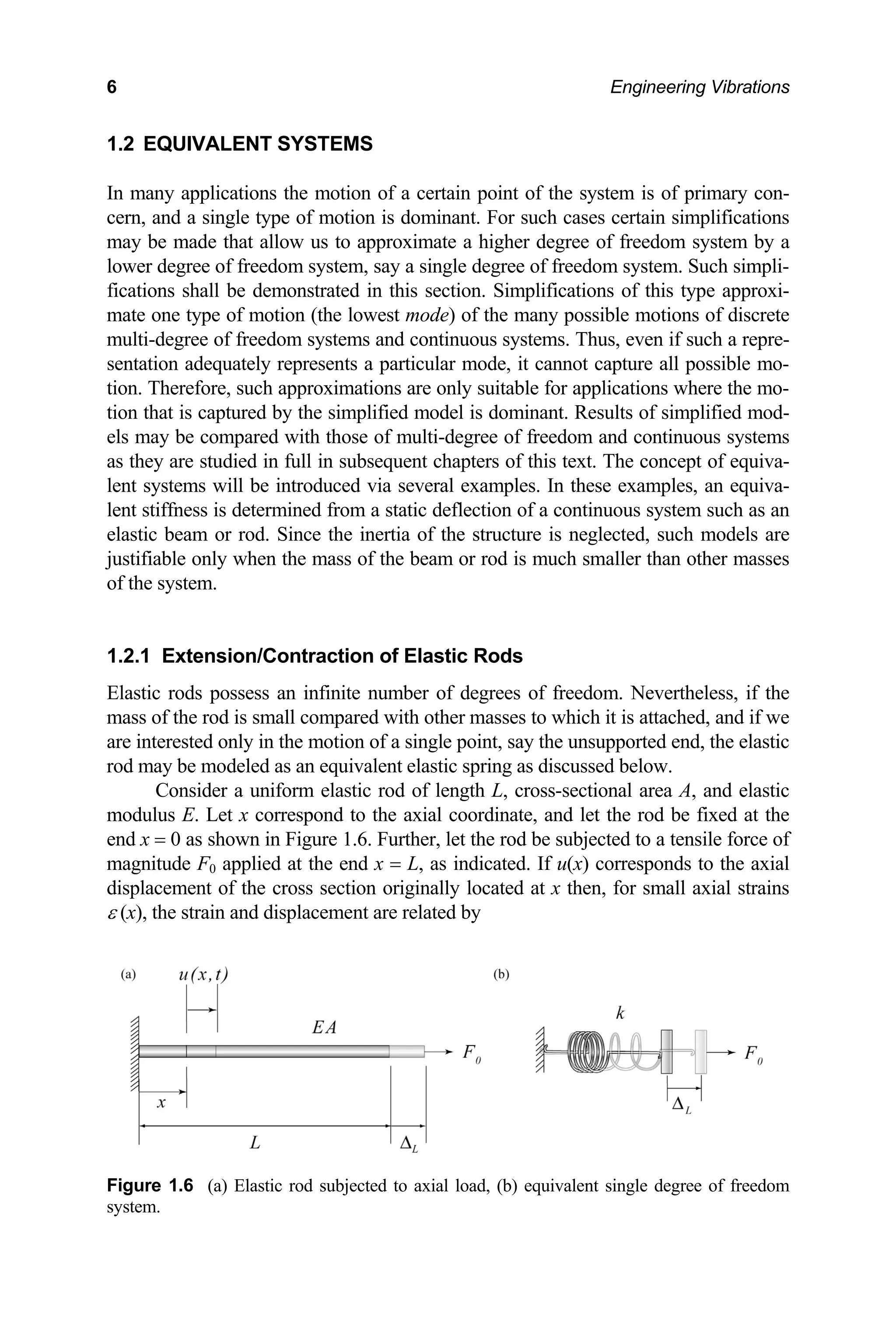
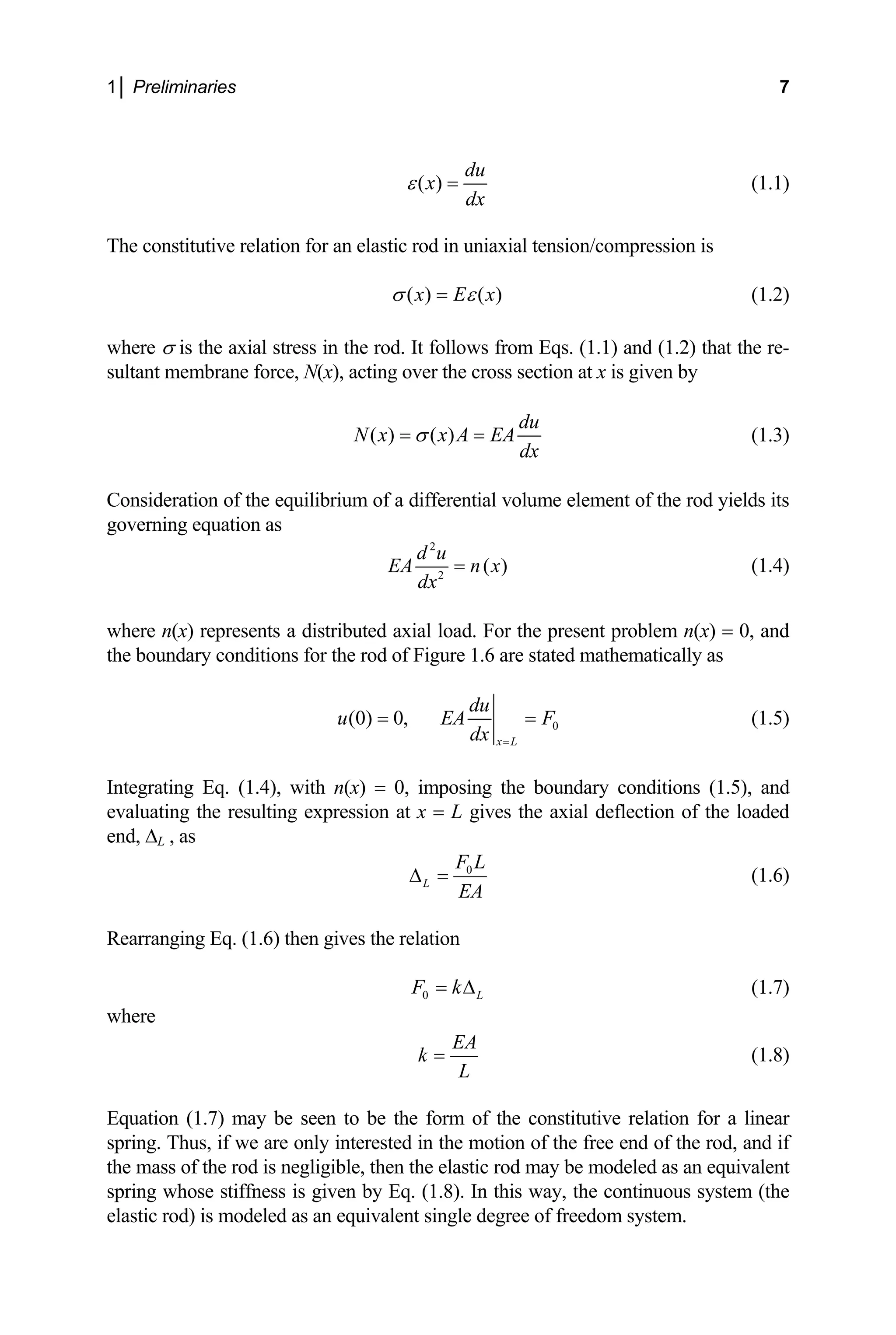
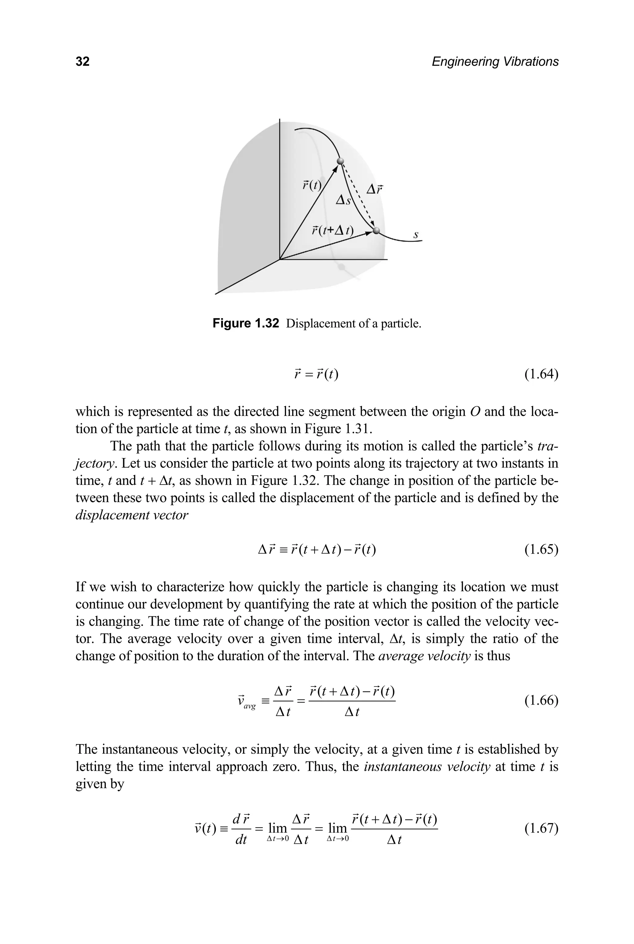
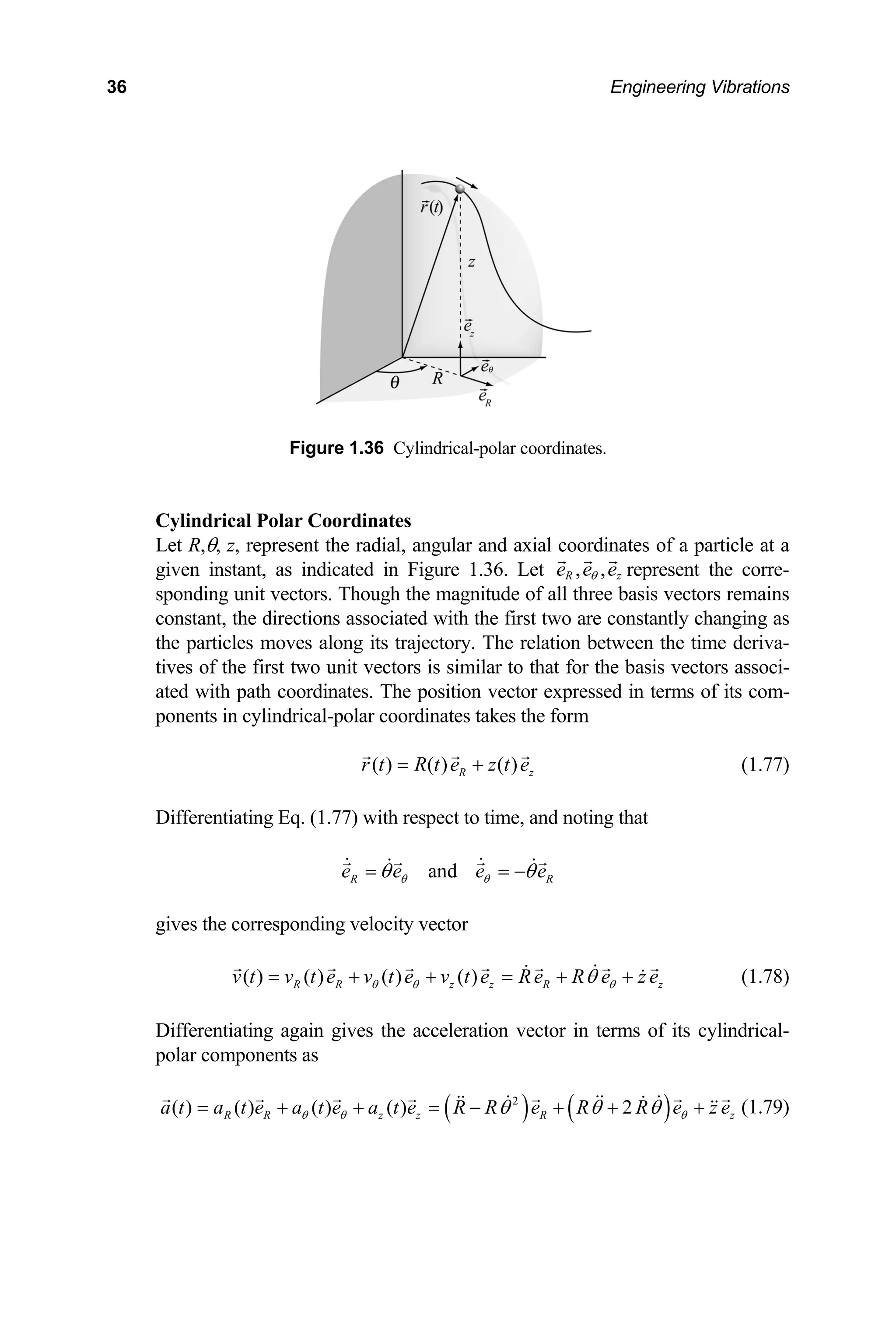
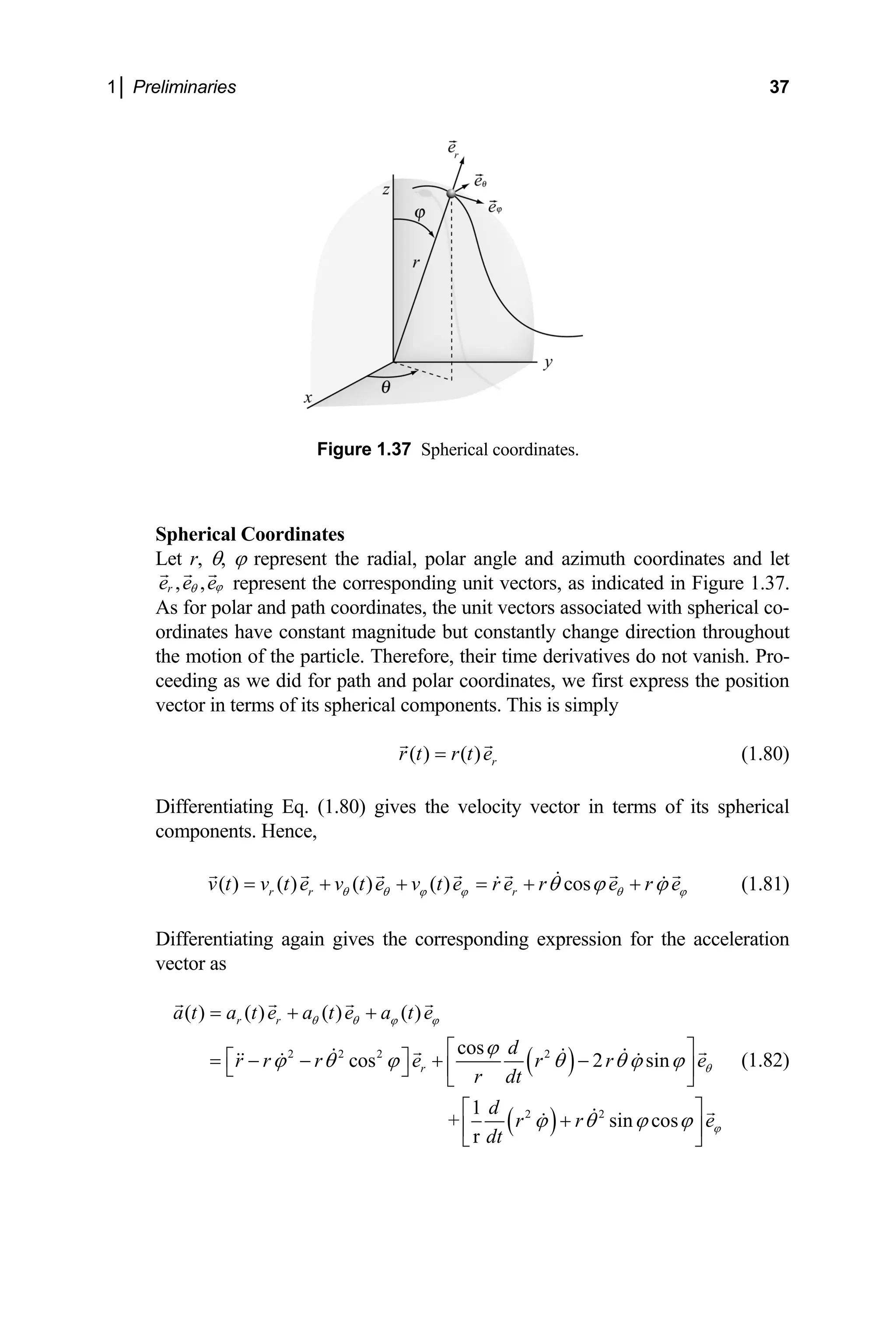
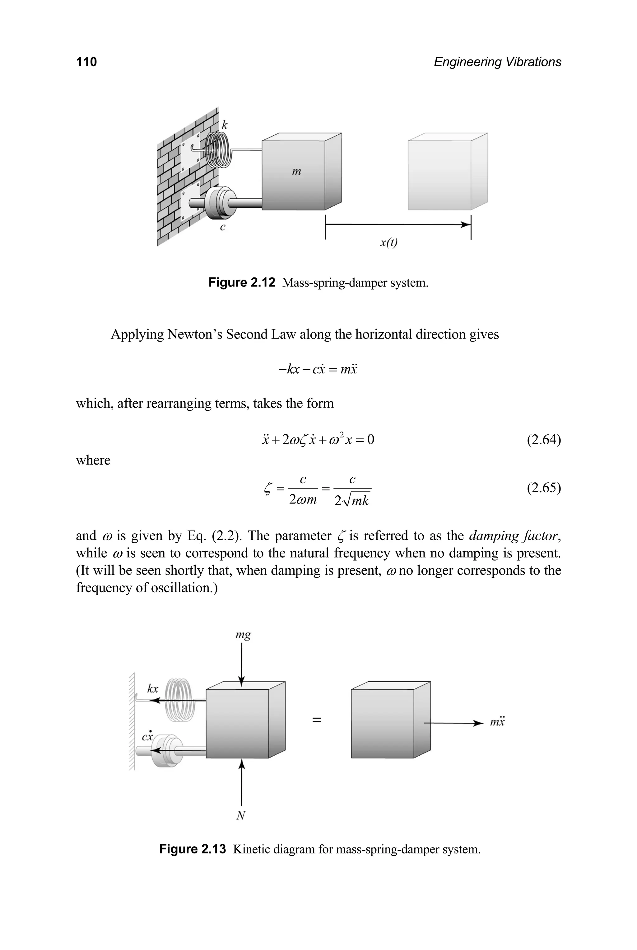
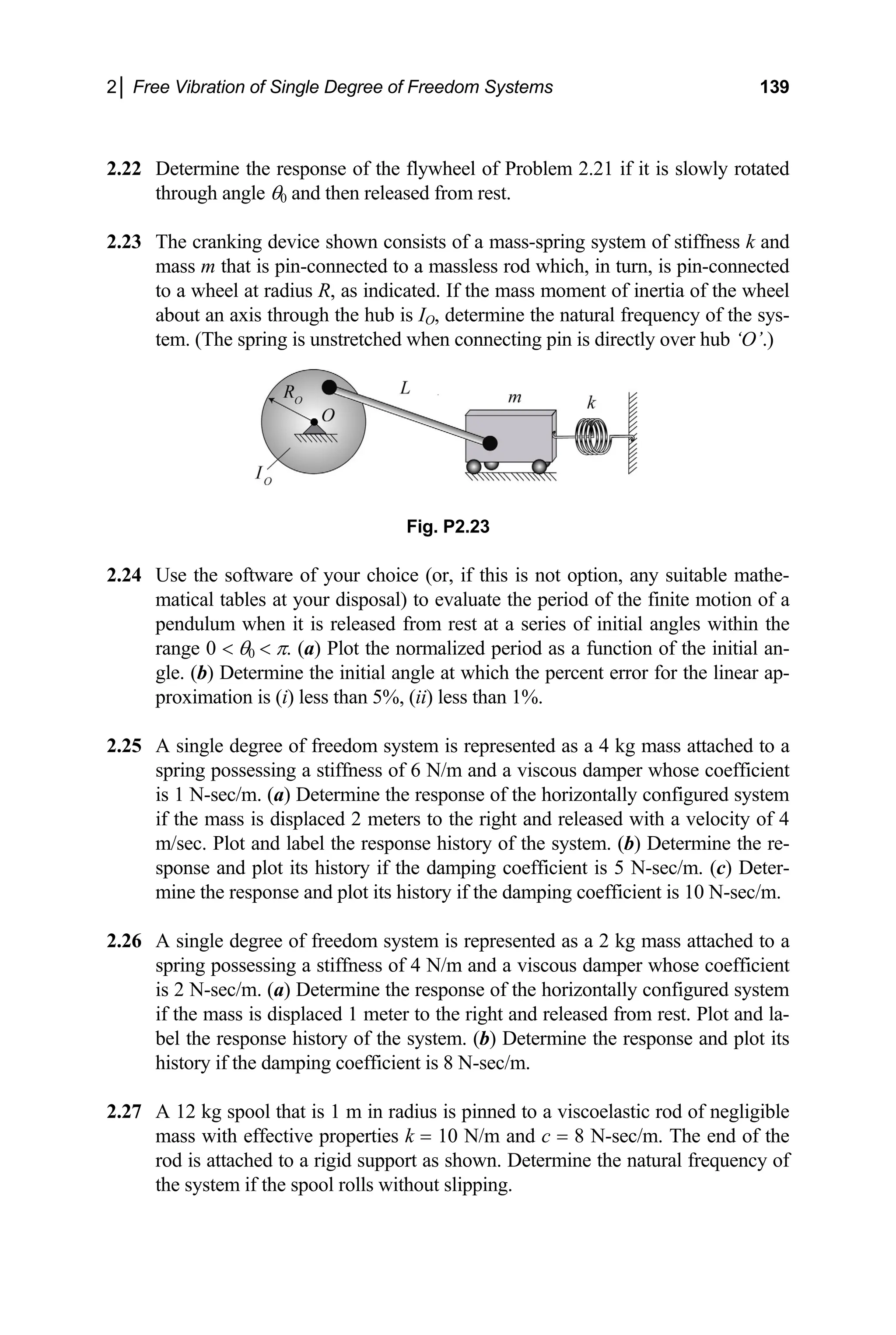
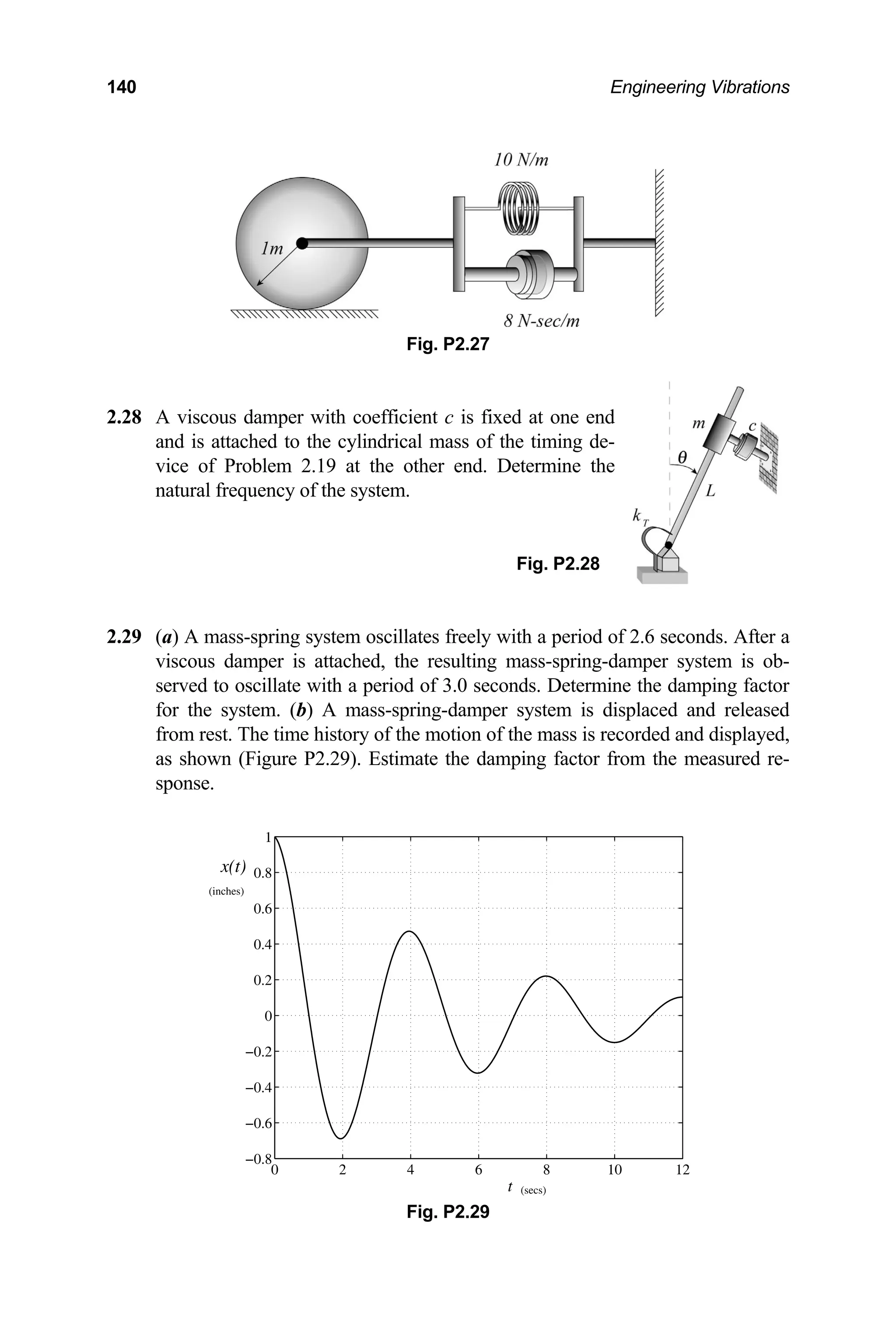
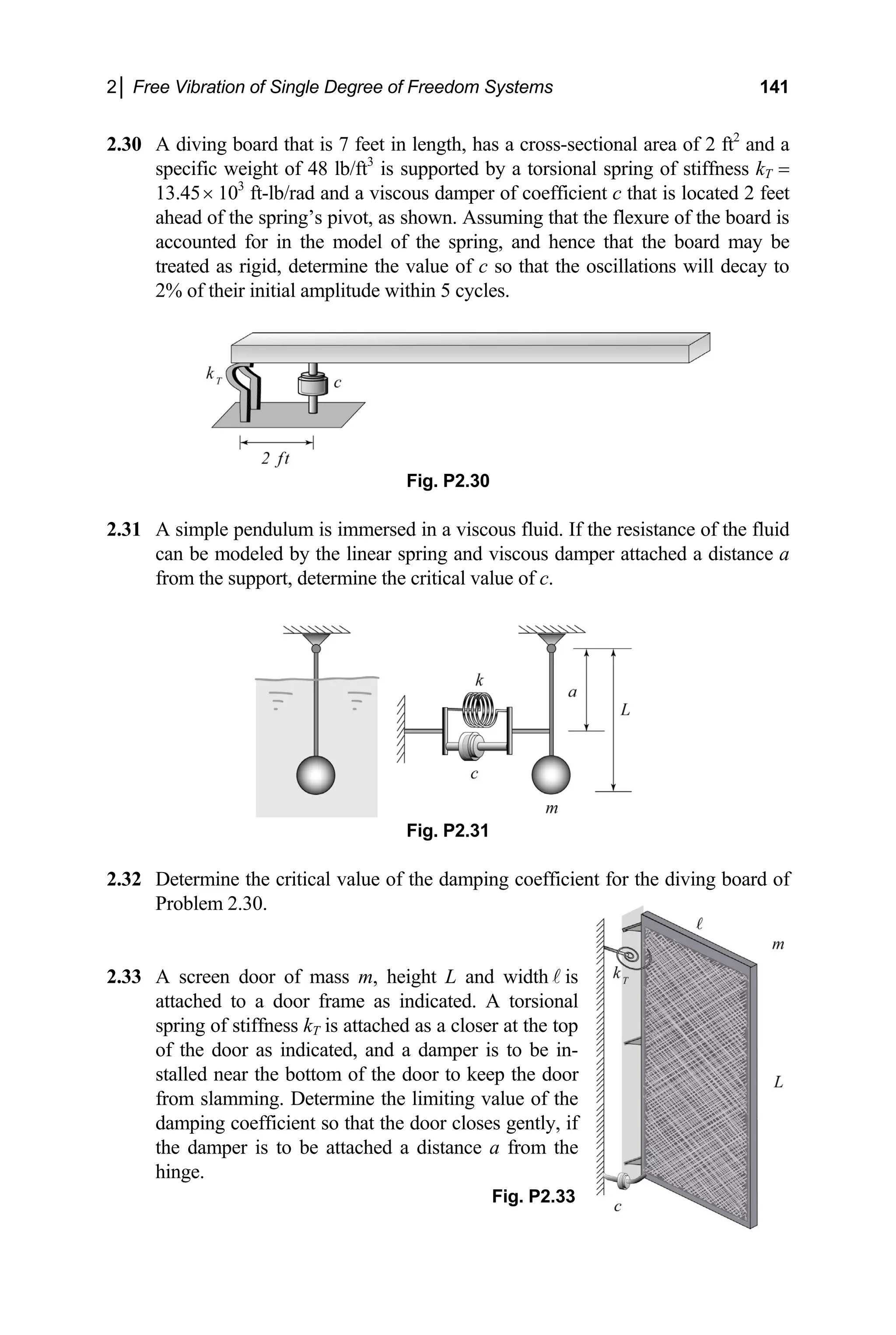
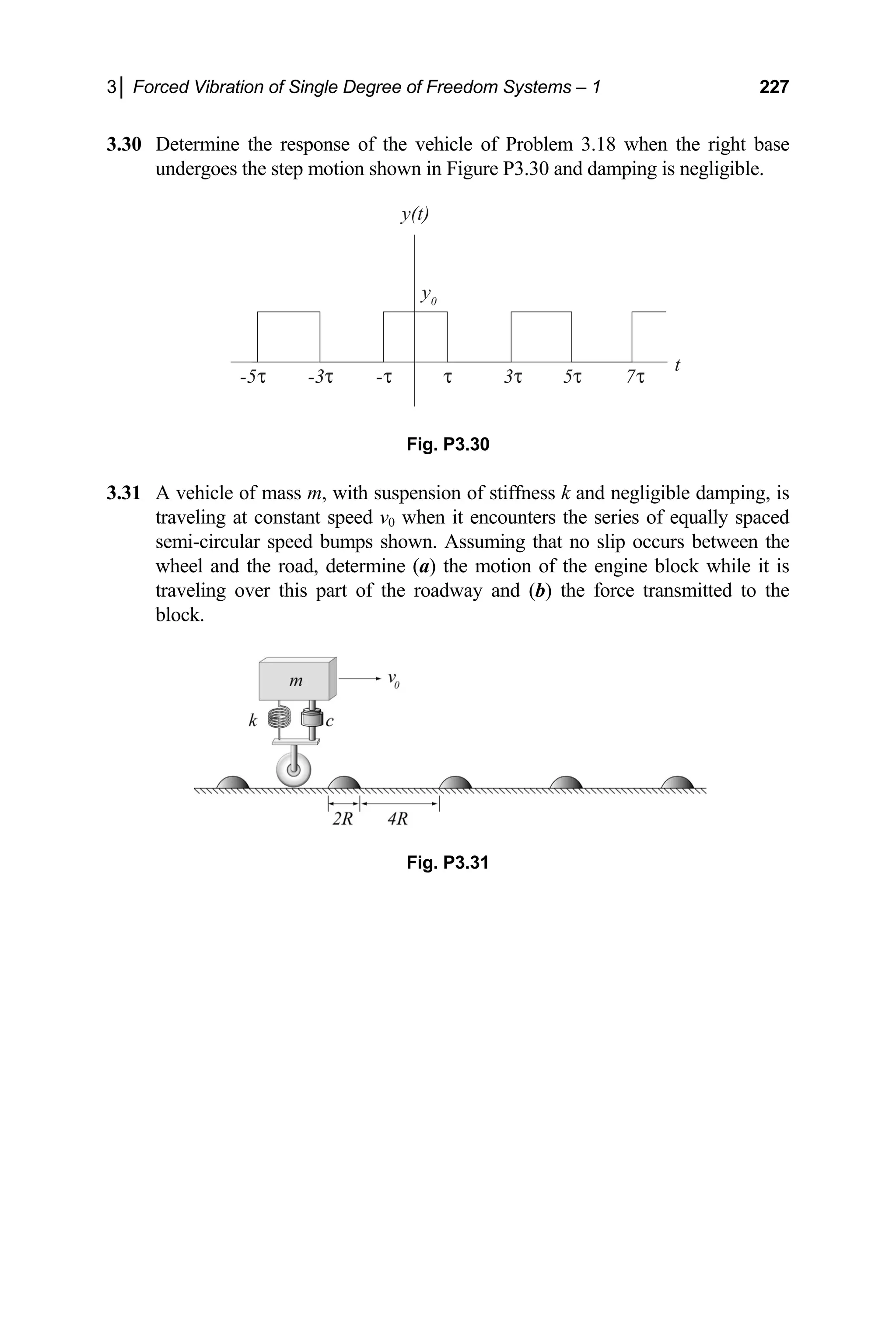
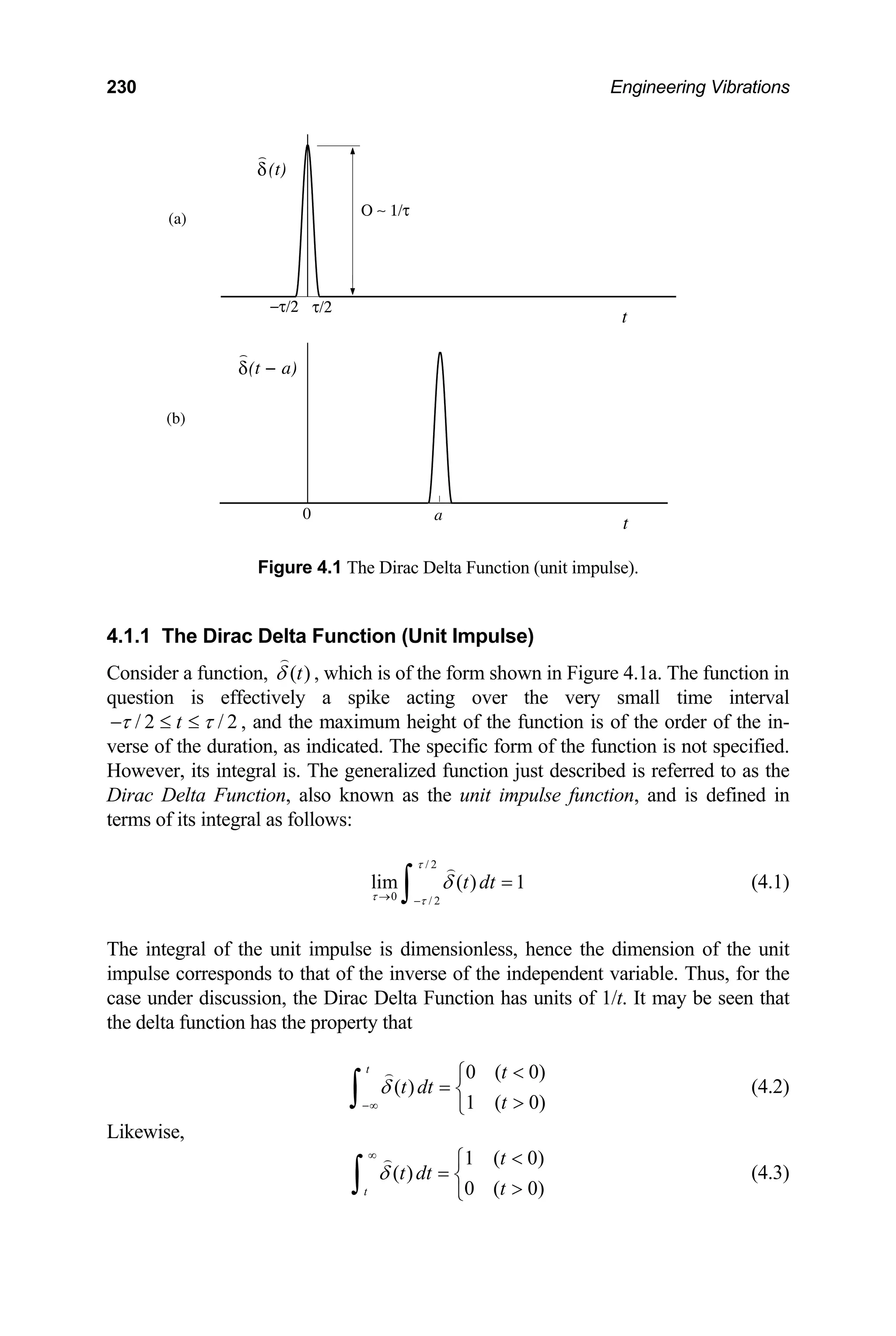
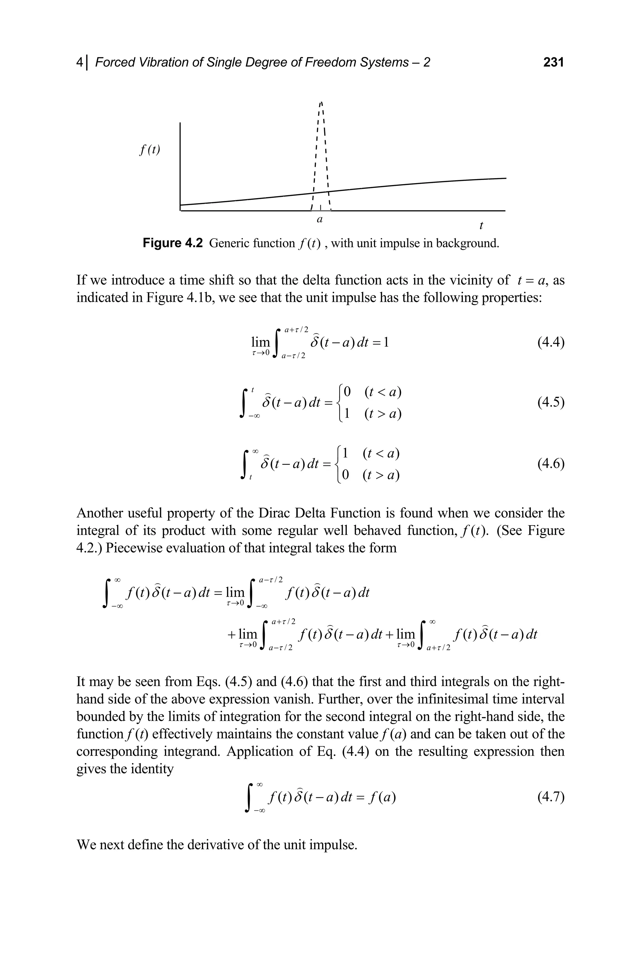
The document is a comprehensive textbook on engineering vibrations authored by William J. Bottega, designed for advanced undergraduate and graduate engineering students. It provides an in-depth look at mechanical and structural vibrations, emphasizing both mathematical development and physical interpretation, and includes extensive examples, exercises, and illustrations. The text covers a wide range of topics, from single degree of freedom systems to multi-degree of freedom systems and one-dimensional continua, making it a resource for foundational study and research in the field.


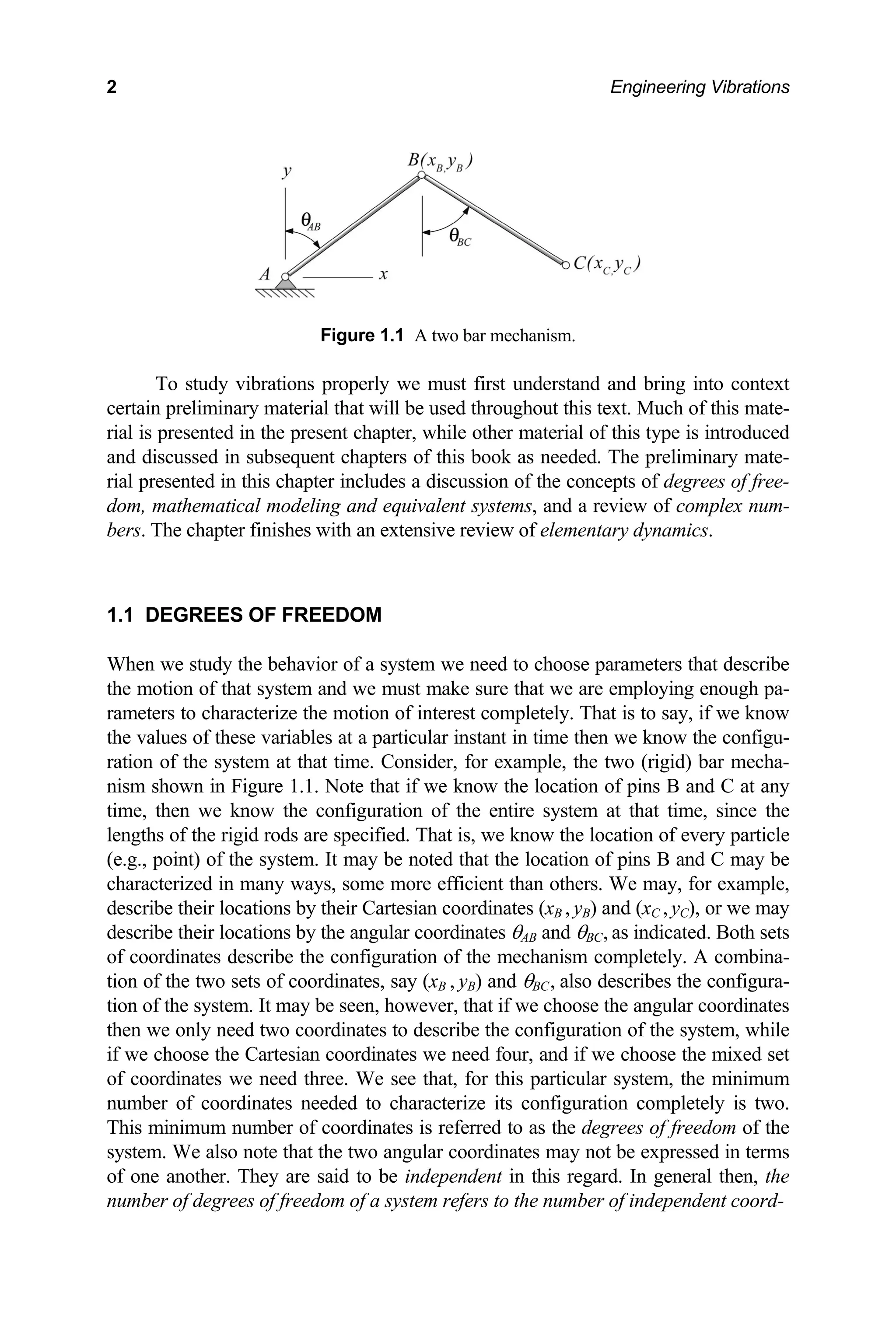
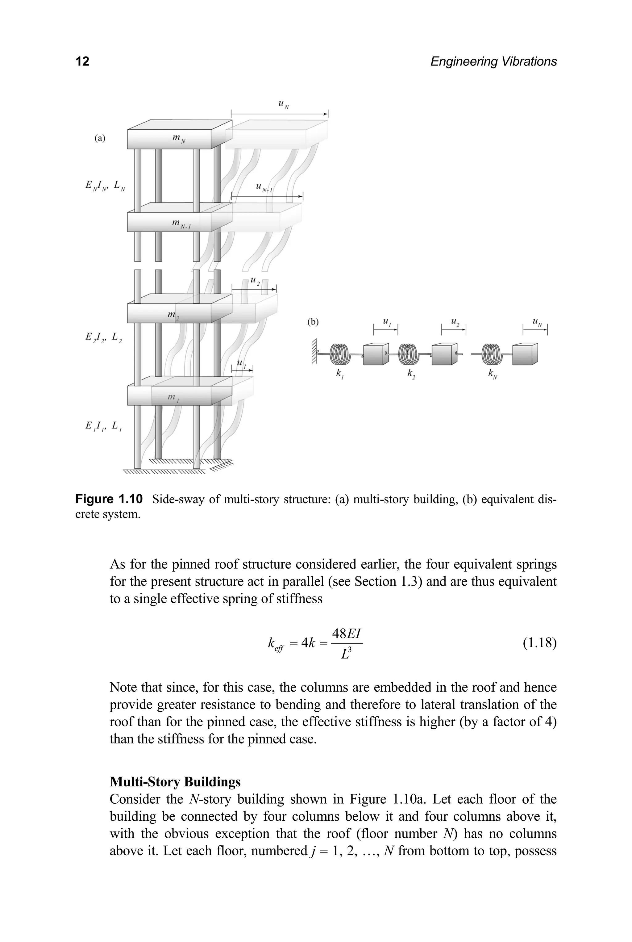
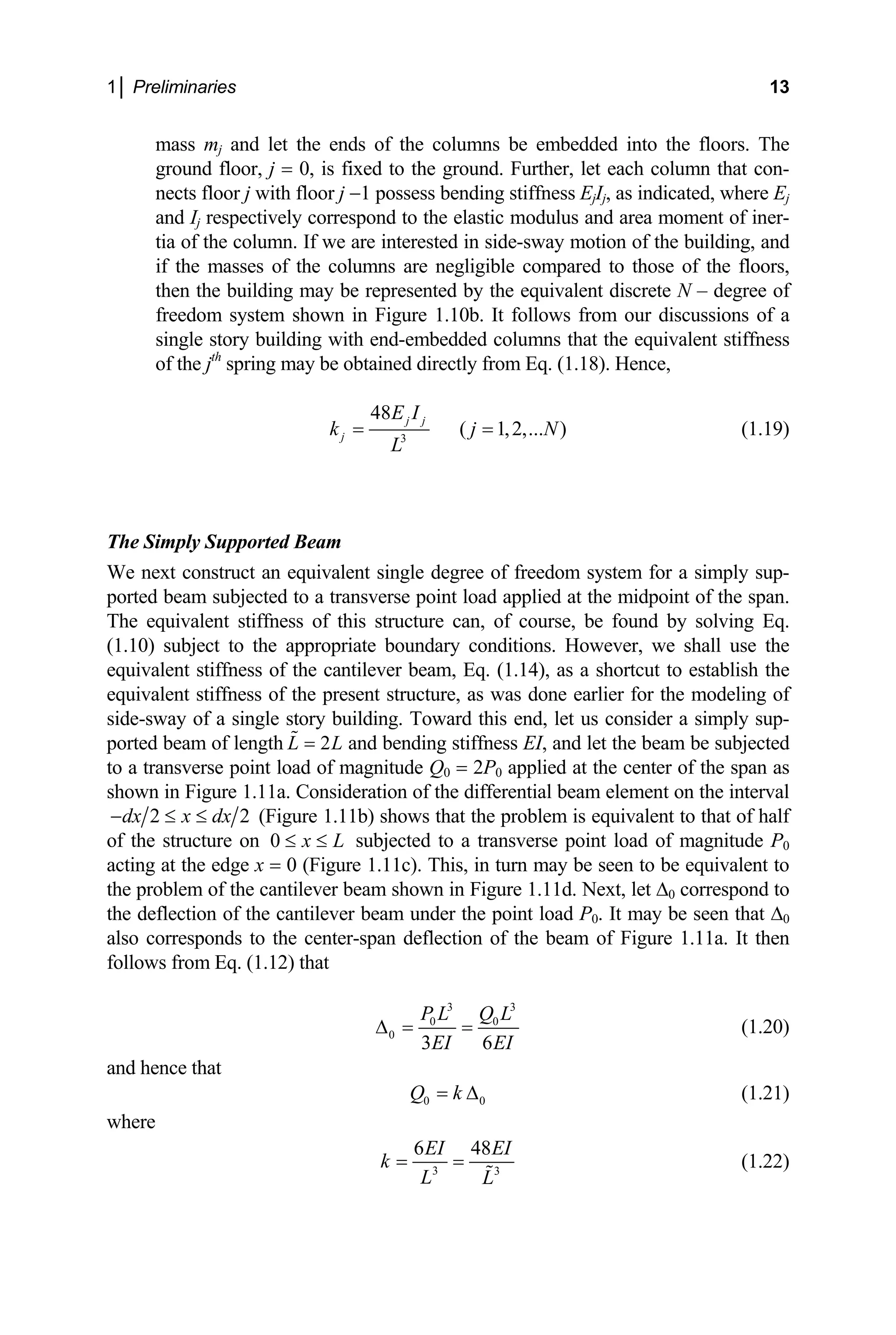
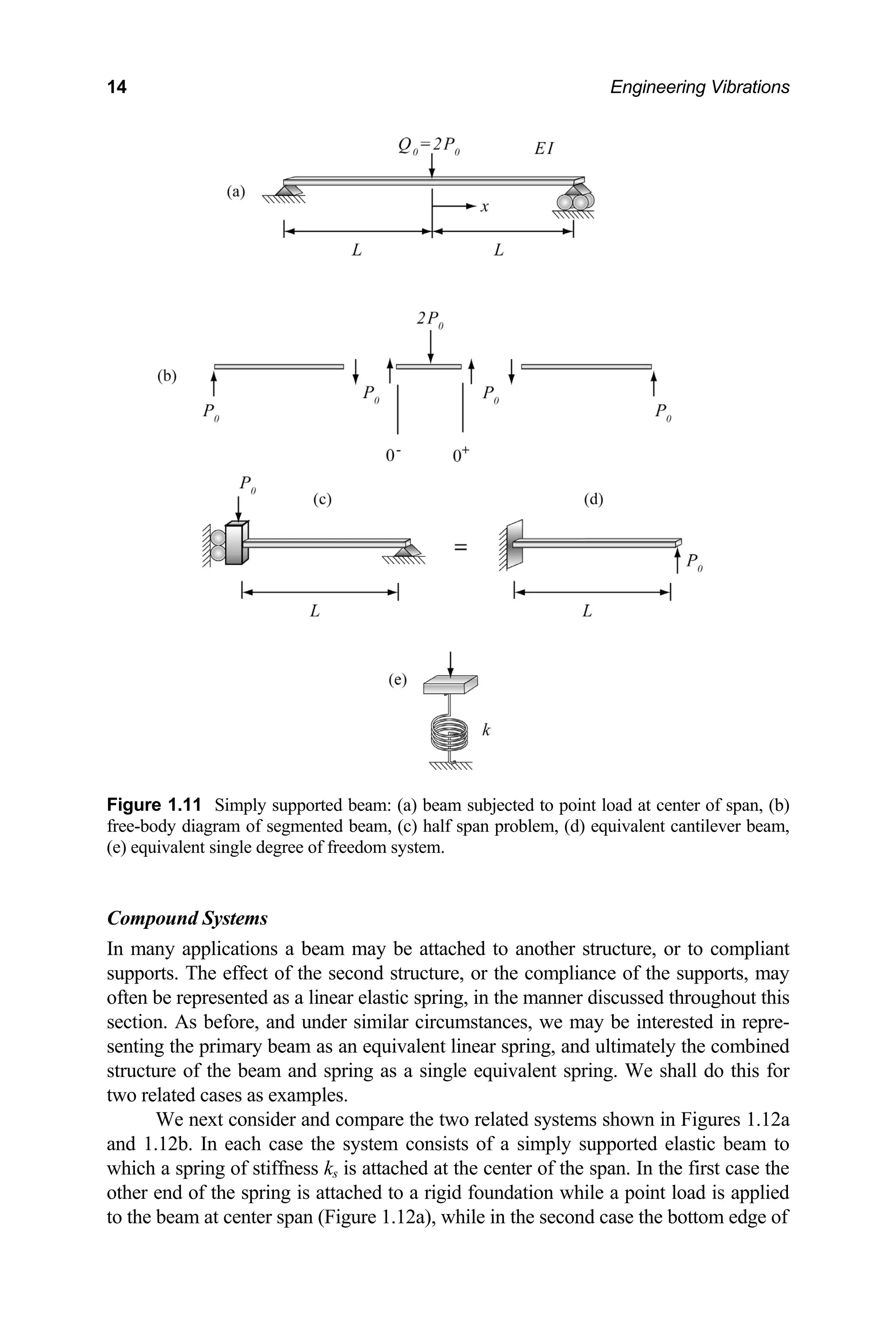
![1│ Preliminaries 39
is the
to pos
work done by the applied force in moving the particle from position 1 1
( )
r r t
≡
ition 2 2
( )
r r t
≡ , t1 and t2 are the times at which the particle is at these positions,
2
(1.86)
1
2
mv
≡
T
is the en
terms
tial, n
kinetic ergy of the particle, and vj = v(tj). It is instructive to write Eq. (1.85) in
of path coordinates. Hence, expressing the resultant force in terms of its tangen-
ormal and binormal components, noting that t
dr dse
= , substituting into Eq.
) and carrying through the dot product gives
(1.85
2
[
2
s s
] ( )
1 1
t t n n b b t t
s s
F e F e F e dse F ds
+ + =
∫
=
∫ i (1.87)
here 1 1 2 2 from Eq. (1.87) that only the tangential com-
force in
oving the particle from position 1 to position 2 is independent of the particular path
along which the particle moves. Let us denote this force as
W
s = s(t ) and s = s(t ). It is seen
w
ponent of the force does work.
Path Dependence, Conservative Forces and Potential Energy
Let us consider a particular type of force for which the work done by that
m
( )
C
F . The work done by
such a force,
2
1
( ) ( )
r
C C
r
F dr
≡
∫ i
W (1.88)
is thus a function of the coordinates of the end points of the path only. If we denote
is function as − U, where we adopt the minus sign
2
1
2
( )
2
( )
r
C
r
r
F dr s
th for convention, then
[ ]
1
( )
s
= − −
∫
1
r
dr
= −∆
= − ∇
∫
i
i
U U
(1.89)
here is the gradient operator. Comparison of the integrals on the right and left
and sides of Eq. (1.89) gives the relation
U
U
w ∇
h
( )
C
F = −∇ U (1.90)
It is seen from Eq. (1.90) that a force for which the w e is independent of the
path traversed is derivable from a scalar potential.
ork don
Such a force is referred to as a con-
rvative force, and the corresponding potential function as the potential energy.
se](https://image.slidesharecdn.com/engineeringvibrations-240713005818-b85f16c0/75/Engineering-Vibrations-Engineering-Vibrations-61-2048.jpg)
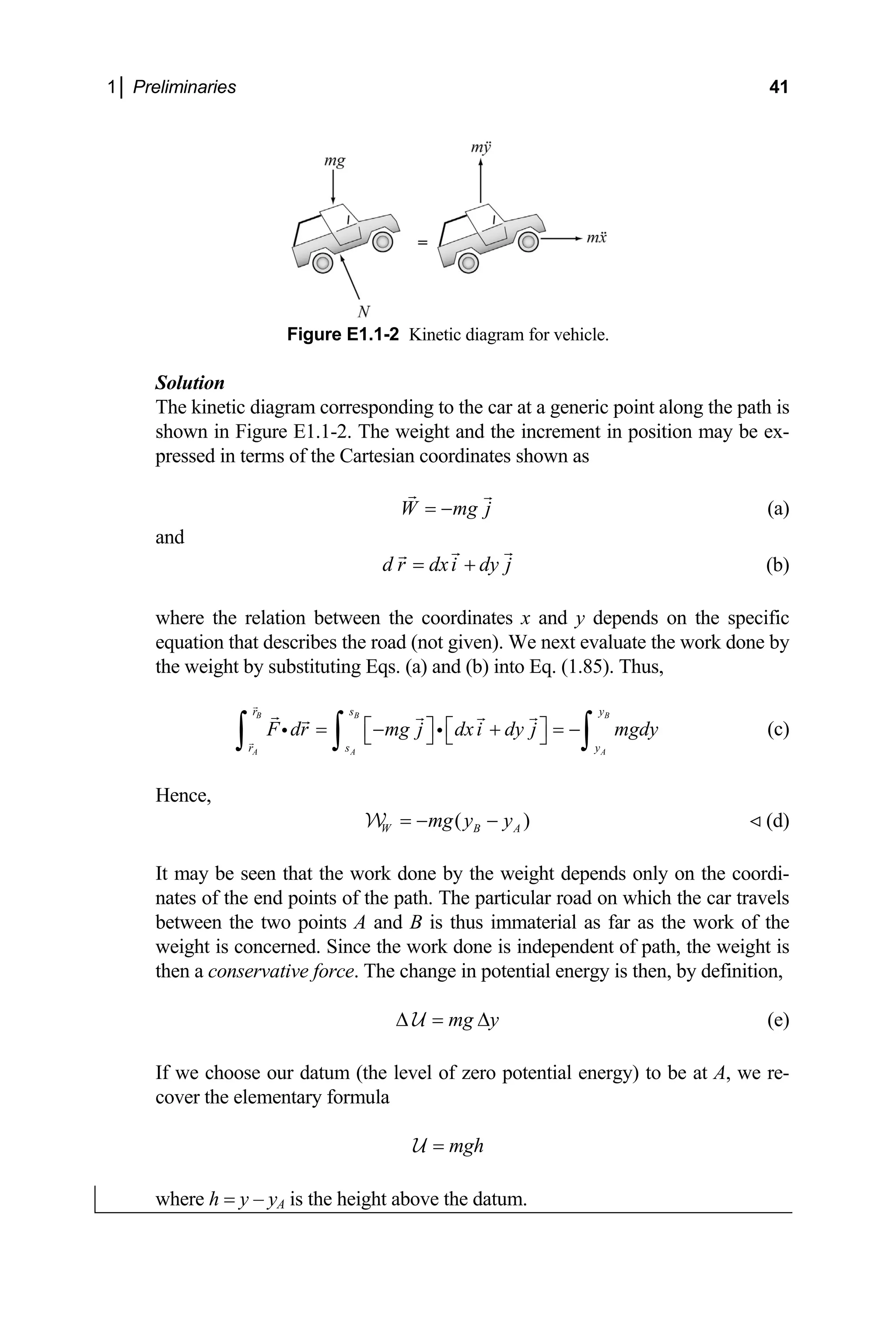
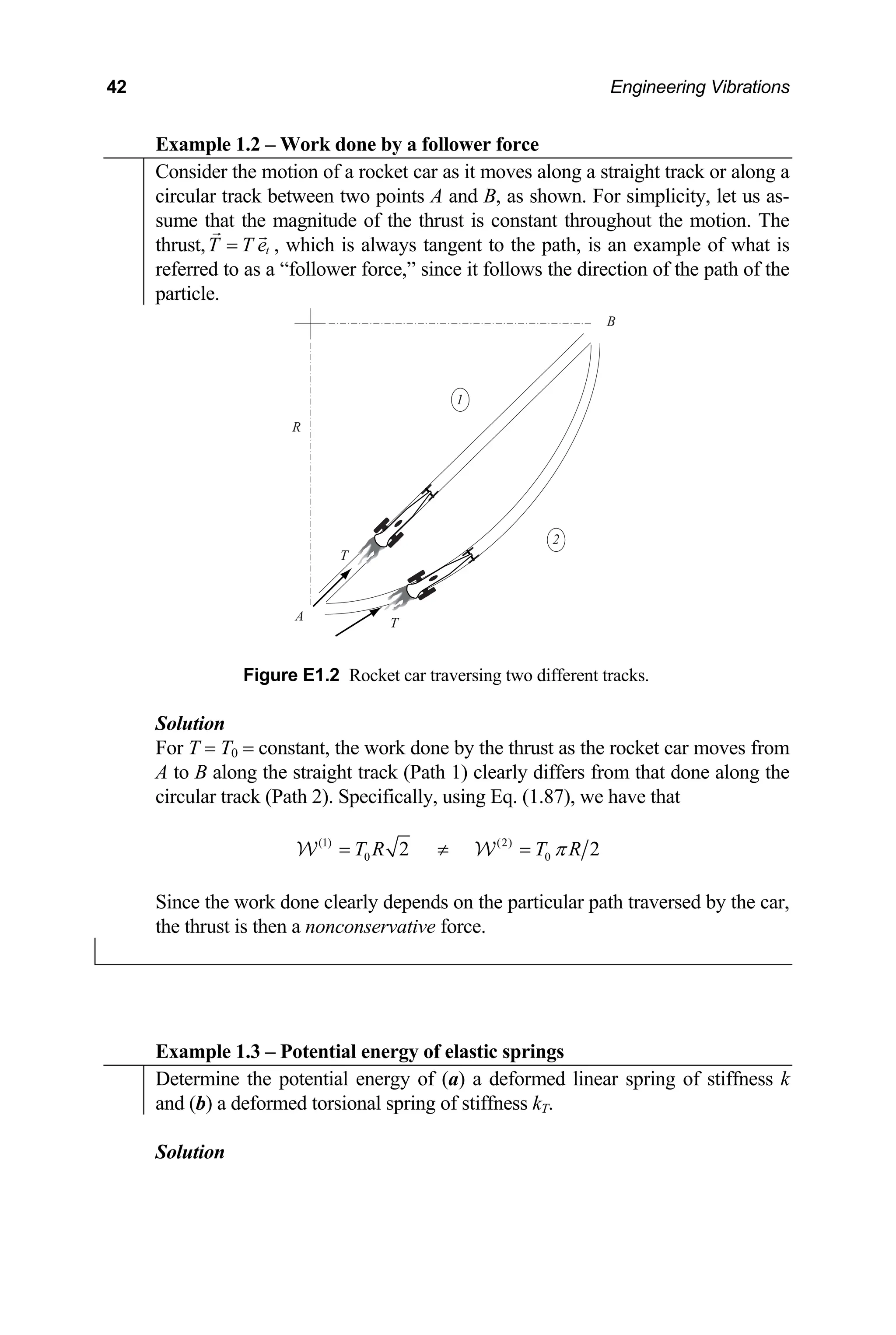
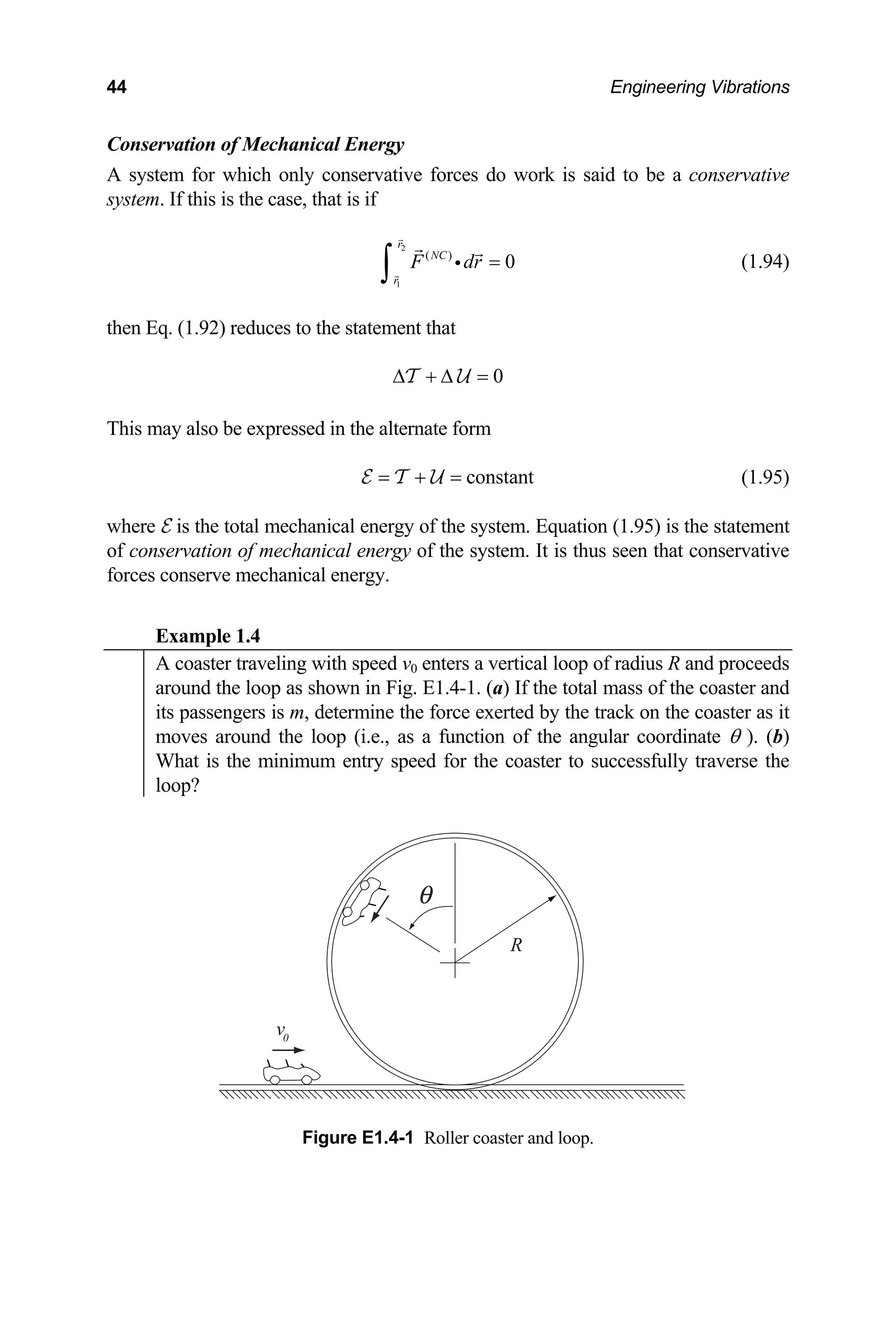
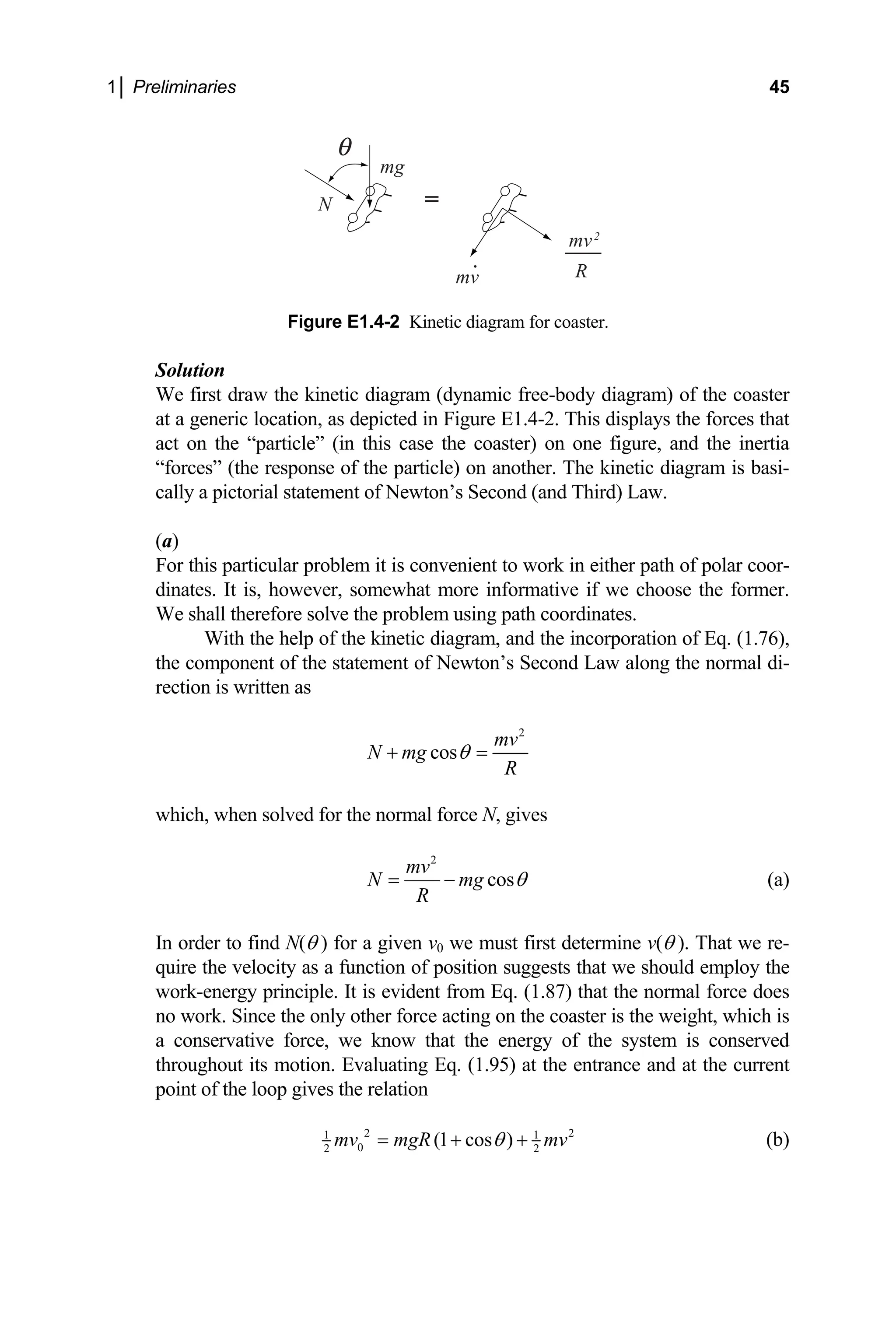
![1│ Preliminaries 43
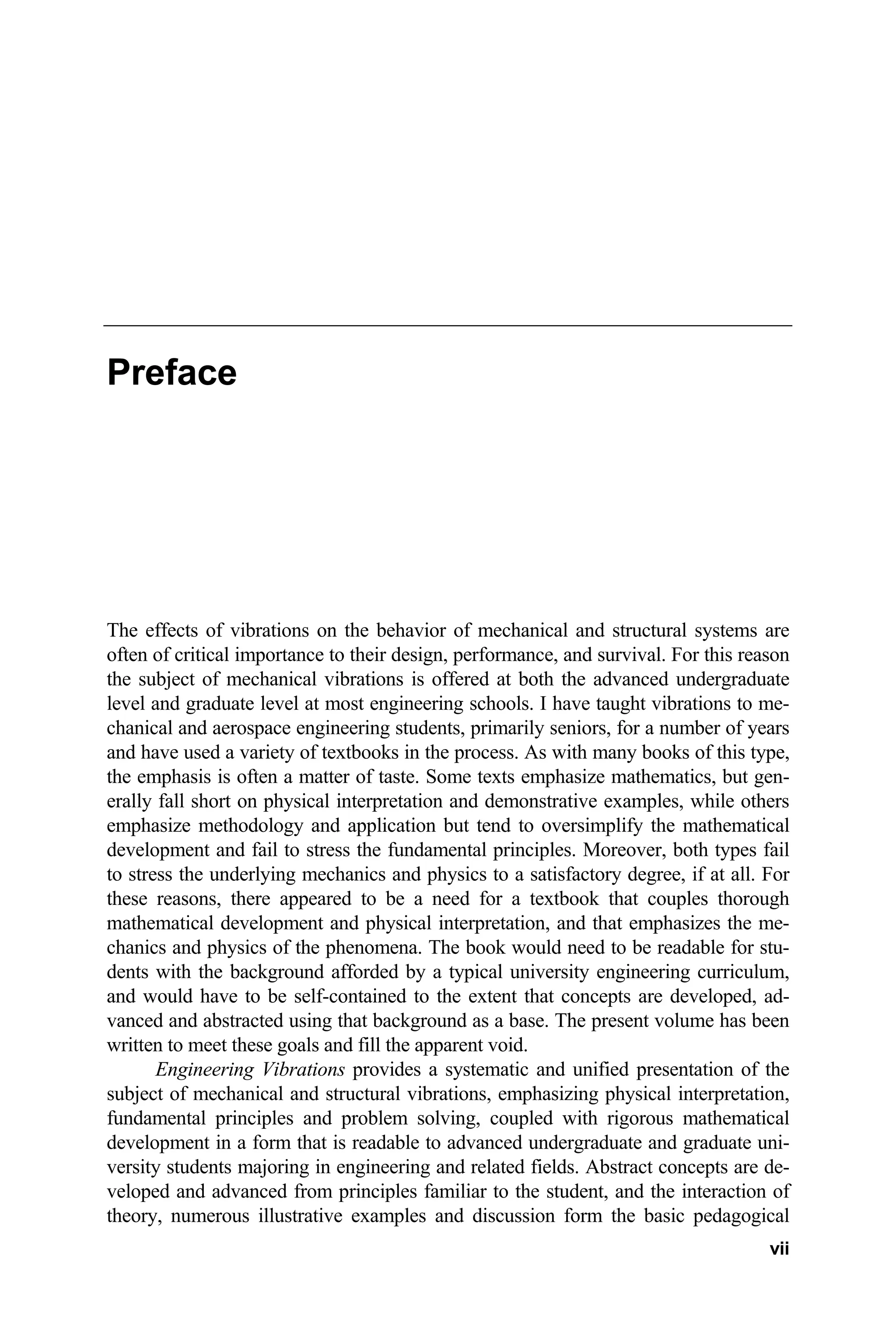
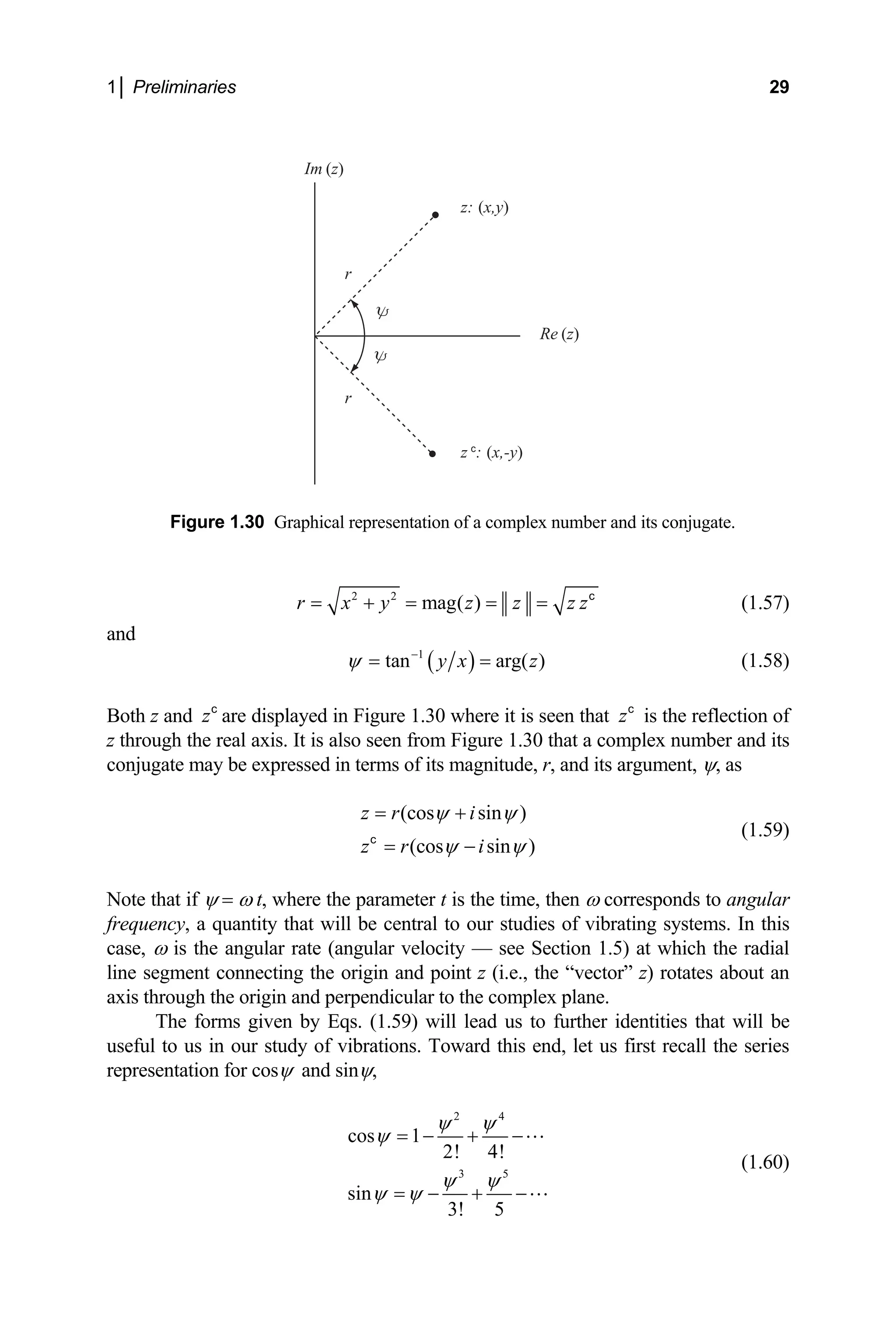
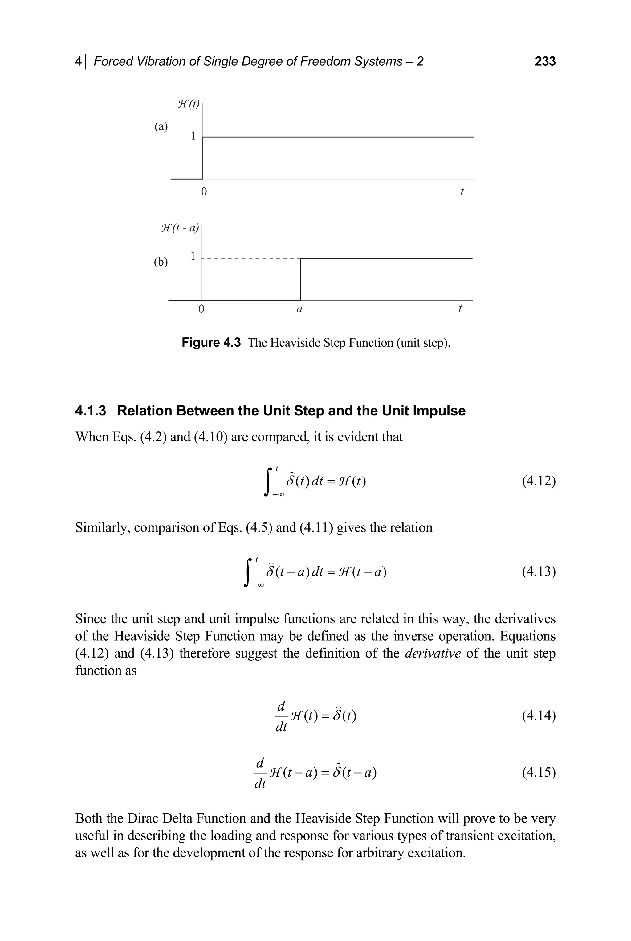
Figure E1.3 Displacement and restoring action: (a) linear spring, (b) torsional spring.
)
s stretched from
nce (unstretched) configuration to the current configuration is readily
(a
The work done by the restoring force of a linear spring as it i
the refere
evaluated as
( ) 2
1
2
0
s
s
ks ds ks
= − = −
∫
W (a)
s is the stretch in the spring (Figure E1.3a). The
where
e
corresponding potential
nergy of the deformed spring is then, from Eq. (1.89),
( ) 2
1
s
ks
= 2
U (b)
ote that it is implicit in the above expression that the datum is chosen as the
ndeformed state of the spring [as per the lower limit of integration of Eq. (a)].
torque and then using Eq.
nce,
N
u
(b)
The potential energy of the deformed torsional spring is similarly determined
y first calculating the work done by the restoring
b
(1.89). He
( ) 2
1
2
0
TS
T T
k d k
θ
θ θ θ
= − = −
∫
W (c)
and
( ) 2
1
2
TS
T
k θ
=
U (d)
where it is implicit that that the datum is taken as the undeformed state of the
torsional spring.](https://image.slidesharecdn.com/engineeringvibrations-240713005818-b85f16c0/75/Engineering-Vibrations-Engineering-Vibrations-65-2048.jpg)
![1│ Preliminaries 47
is the
partic
during
onservation of Linear Momentum
If the linear impulse vanishes over a given time interval, Eqs. (1.96) and (1.97) re-
duce to the statements
linear momentum of the particle at time t. Thus, a linear impulse that acts on a
le for a given duration produces a change in linear momentum of that particle
that time period.
C
2 1
( ) ( )
mv t mv t
= (1.100)
constant
mv
or
℘= = (1.101)
this occurs, the linear momentum is said to be conserved over the given time
.
When
interv
ngular Impulse and Momentum
In the previous section we established an integral, over time, of Newton’s Second
aw that led to the principle of linear impulse-momentum. We next establish the rota-
tional analogue of that principle.
product of Newton’s Second Law, Eq. (1.83), with
al
A
L
Let us form the vector cross
the position vector of a particle at a given instant. Doing this results in the relation
O O
M H
= (1.102)
where
O
M r F
= × (1.103)
is the moment of the applied force about an axis through the origin, and
O
H r mv
= × (1.104)
red to as the angular momentum, or m
. Let us next multiply Eq. (1.102) by the differential time increment dt, and
tegrate the resulting expression between two i
le’s motion. This results in the statement of the
omentum,
t t t t
t
v
is oment of momentum, of the particle
refer
about O
in nstants in time, t1 and t2, during the
partic Principle of Angular Impulse-
M
[ ] [ ]
2
t
r F dt r m r mv
2 1
1
= =
× = × − ×
∫ (1.105)
r, equivalently,
o
O O
H
= ∆
J (1.106)
where](https://image.slidesharecdn.com/engineeringvibrations-240713005818-b85f16c0/75/Engineering-Vibrations-Engineering-Vibrations-69-2048.jpg)
![48 Engineering Vibrations
O
F
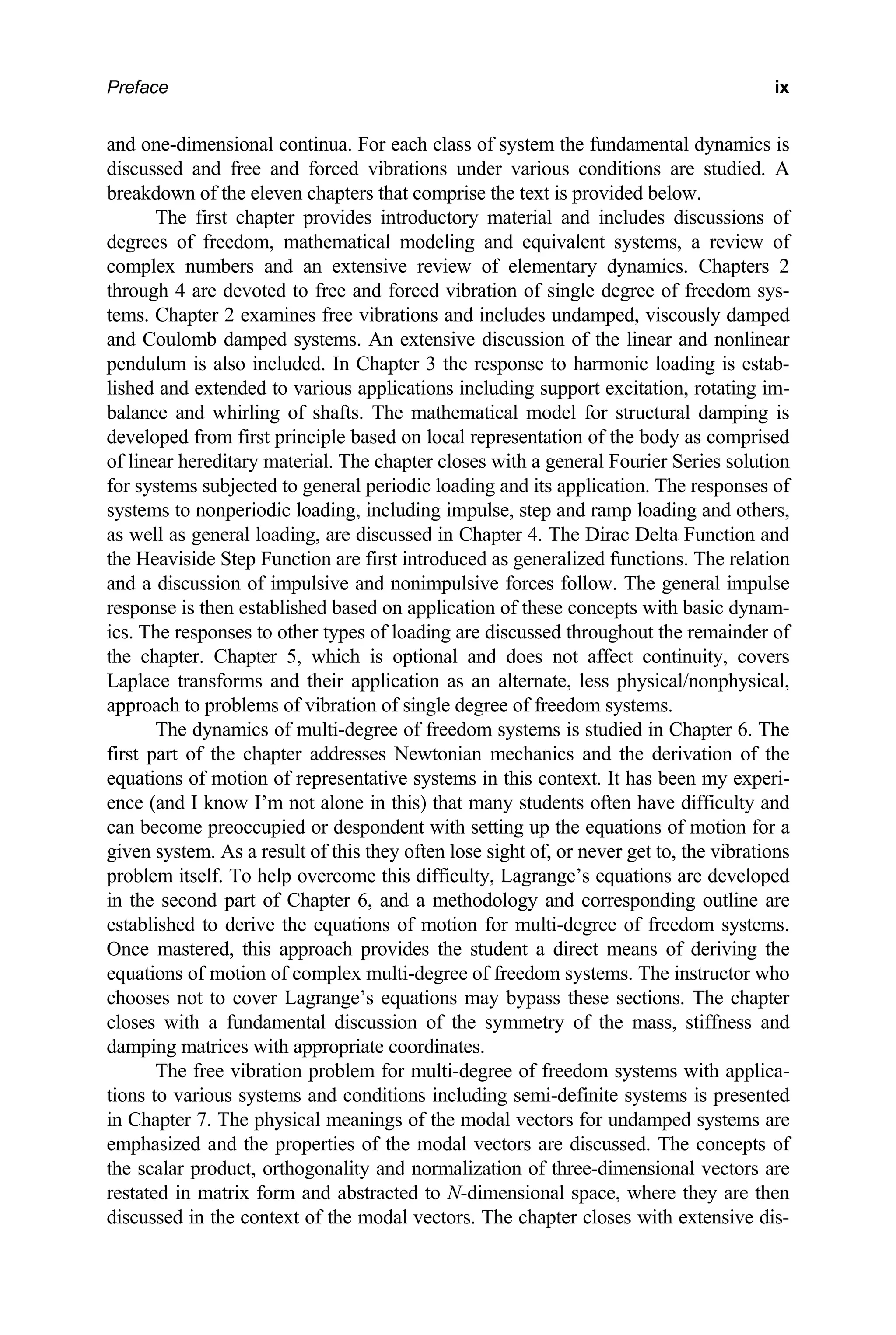
Figure 1.38 Central force motion.
2 2
1 1
t t
O O
t t
M dt r F dt
≡ = ×
∫ ∫
J (1.107)
is the angular impulse about an axis through O, imparted by the force F , or simply
the angular impulse about O. The angular impulse is seen to be the impulse of the
oment o
m f the applied force about the origin.
m
Conservation of Angular Momentu
If the angular impulse about an axis vanishes, then Eqs. (1.105) and (1.106) reduce to
the equivalent statements
[ ] [ ]
2 1
t t t t
r mv r mv
= =
× = × (1.108)
or
constant
O
H r mv
= × = (1.109)
e given time interval. When this is so, the angular momentum is said to be
onserved about an axis through O. It should be
e conserved about an axis through one point and not anoth
Figure 1.39 System of N particles.
over th
c noted that angular momentum may
er. An example of this is
b
when a particle undergoes central force motion, where the line of action of the ap-
lied force is always directed through the same point (Figure 1.38).
p
Fp
rp
rG
fpq
mp
m1
mq
m2
mN
G
fqp
rp/G](https://image.slidesharecdn.com/engineeringvibrations-240713005818-b85f16c0/75/Engineering-Vibrations-Engineering-Vibrations-70-2048.jpg)
![54 Engineering Vibrations
N
O p p
M r F
1
p=
≡ ×
∑ (1.138)
p
and
1
N
O p p
p
H r m v
=
≡ ×
∑ (1.139)
spectively correspond to the resultant moment of the external forces about O, and
stants in time, we obtain the Principle of Angular Impulse-
omentum for the particle system,
re
total angular momentum of the system about an axis through O.
If we next multiply Eq. (1.137) by the differential time increment dt, and inte-
grate between two in
M
2
1
2 1
( ) ( )
t
O O O
t
M dt H t H t
= −
∫ (1.140)
or, in expanded form,
2
2 1
1
1 1 1
N N N
t
p p p p p p p p
t t t t
t
p p p
r F dt r m v r m v
= =
= = =
⎡ ⎤ ⎡ ⎤
× = × − ×
⎣ ⎦ ⎣ ⎦
∑ ∑ ∑
∫ (1.141)
Proceeding for the center of mass as for a single particle gives the Principle of Angu-
lar Impulse-Momentum for the center of mass of a particle system,
G
t
r F dt [ ] [ ]
2
2 1
1
t
G G G G
t t t t
r mv r mv
= =
× − ×
× =
∫ (1.142)
(1.115) into Eq. (1.141), subtracting Eq. (1.142) from
e resulting expression and incorporating Eq. (1.119) gives the Principle of Angular
pulse-Momentum for motion relative to the center of m
1 1 1
N N N
t
p G p p G p p G t t
t
p p p
r F dt r m v
Substitution of Eqs. (1.114) and
th
Im ass,
/ /
p G p p G t t
r m v
2
2 1
1
/ / / = =
= = =
⎡ ⎤
× = × ⎡ ⎤
− ×
⎣ ⎦
∑ ∑
∫
quations (1.140)–(1.143) are the statements of an
ral particle systems.
⎣ ⎦
∑ (1.143)
E gular impulse-momentum for gen-
e
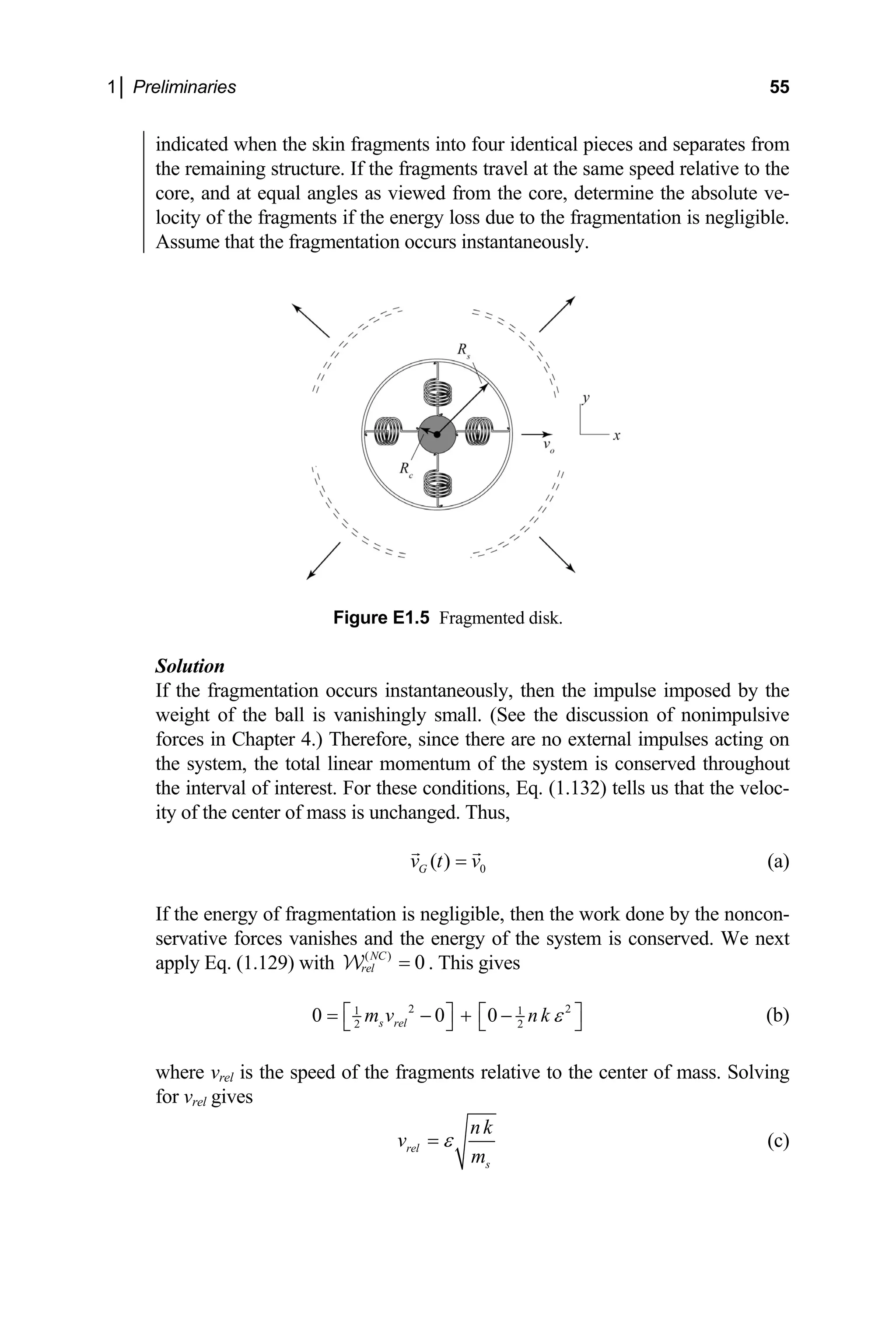
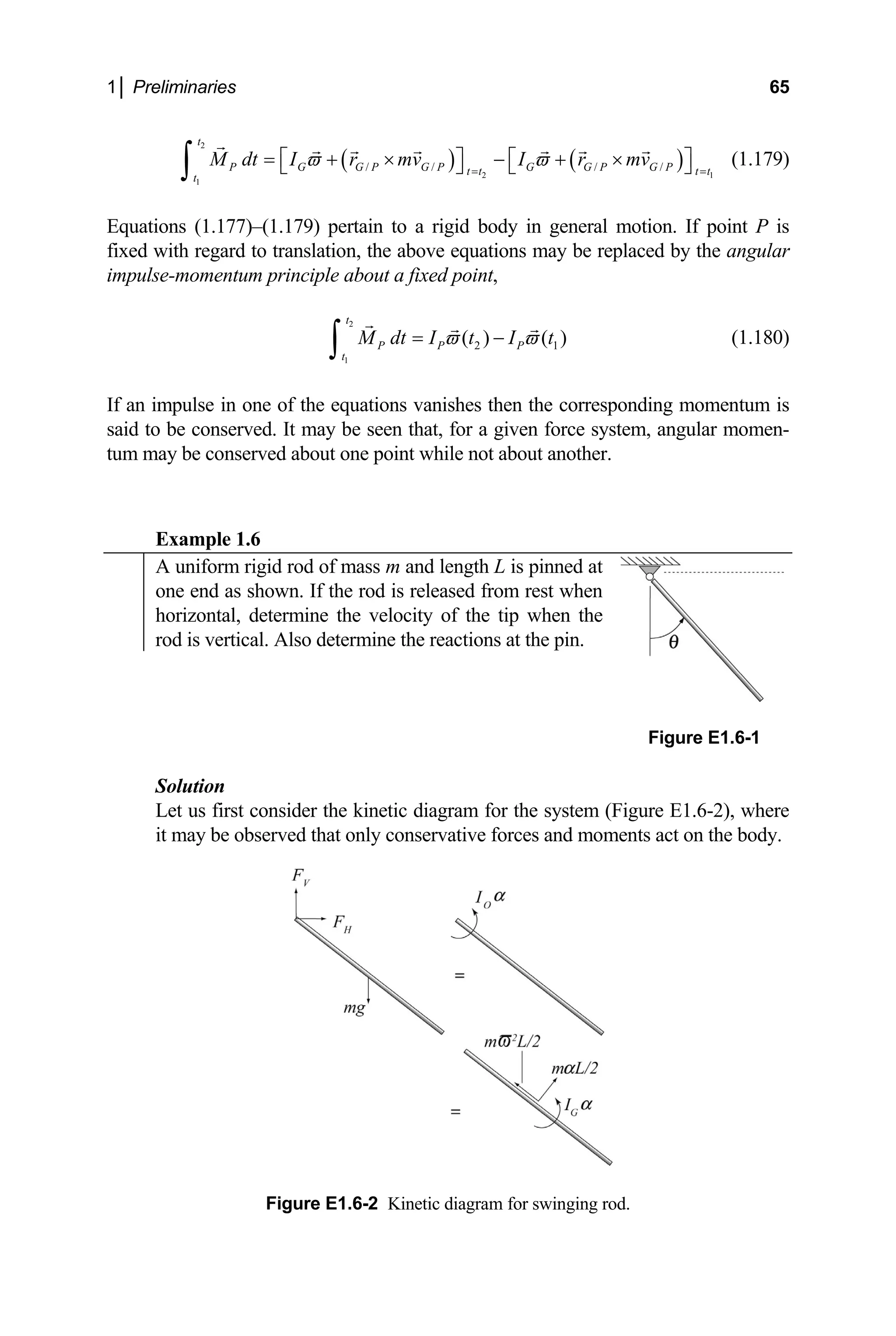
Example 1.5
Consider a circular disk comprised of a skin of mass ms, a relatively rigid core
of mass mc and a compliant weave modeled as n identical linear springs of
k and negligible mass, as shown
stiffness . The length of each spring when un-
stretched is R0 = Rs − Rc − ε. The disk is translating at a speed v0 in the direction](https://image.slidesharecdn.com/engineeringvibrations-240713005818-b85f16c0/75/Engineering-Vibrations-Engineering-Vibrations-76-2048.jpg)
![62 Engineering Vibrations
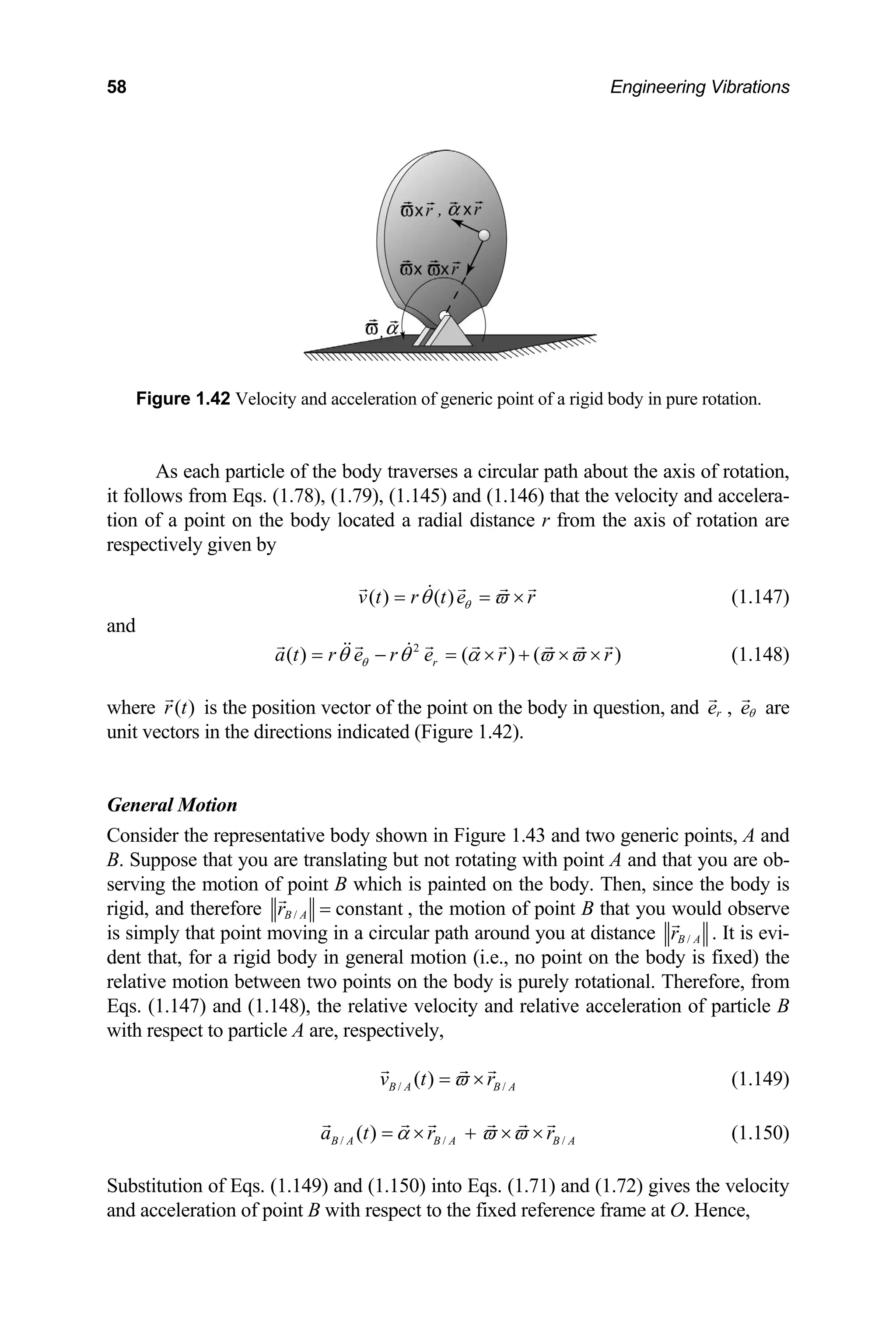
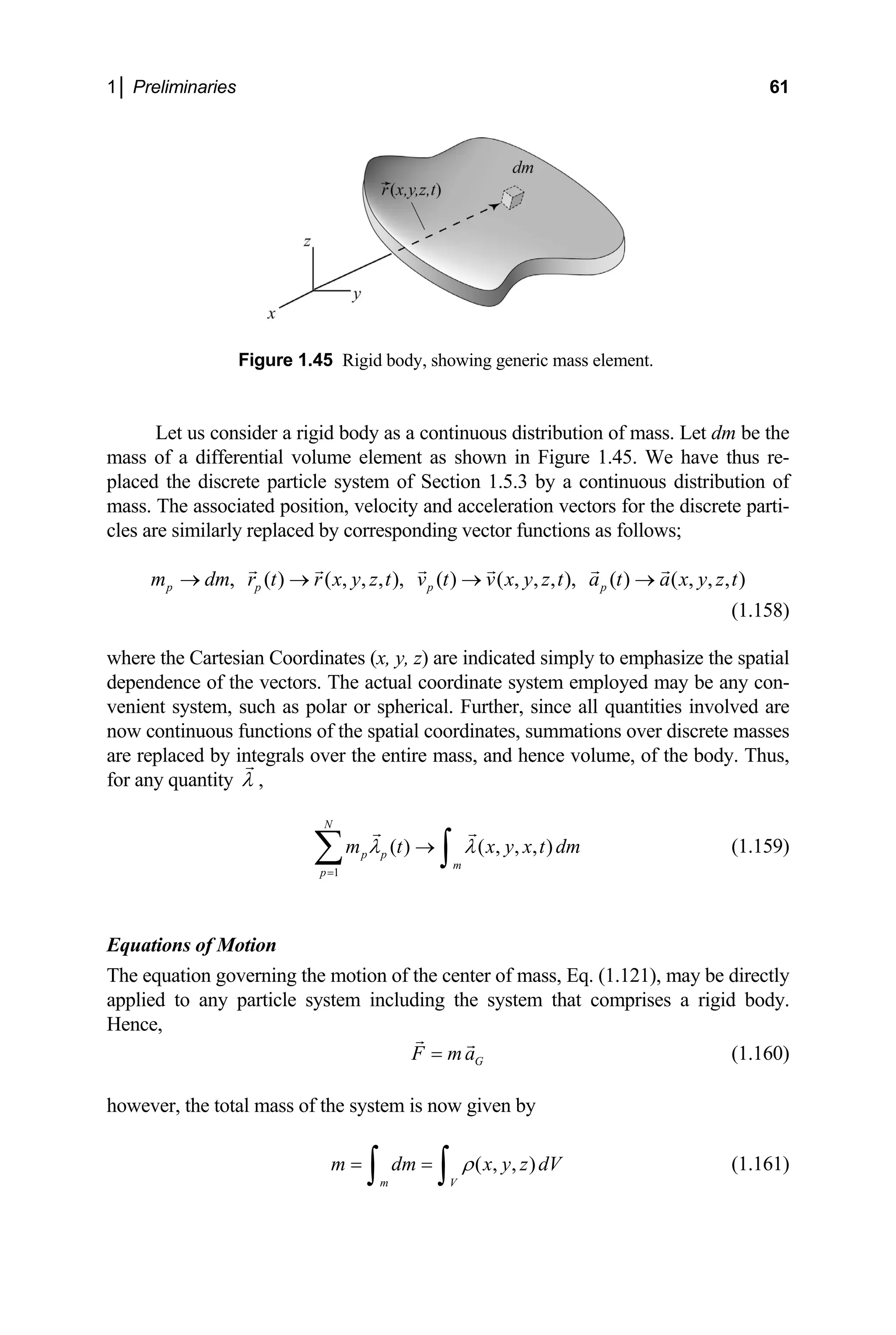
where ρ is the mass density (mass per unit volume) of the body.
Let us next express Eqs. (1.137)–(1.139) in terms of continuous functions using
Eqs. (1.158) and (1.159). Doing this gives the equations governing rotational motion
about the center of mass, and about an arbitrary point P. Hence,
G G
M I α
= (1.162)
[ ]
/
P G G P G
M I r ma
α
= + × (1.163)
where G
M and P
M
ss and the resu
are, respectively, the resultant moment about an axis through the
center of ma ltant moment about an axis through P of the external
forces acting on the body. Further, the parameter
2
G rel
m
I r dm
=
∫ (1.164)
the mass moment of inertia (the second moment of the mass) about the axis though
is
the center of mass of the body, and
( , , ) ( , , )
rel rel
r x y z r x y z
≡
is the distance of the mass element, dm, from that axis.
If one point of the body is fixed with regard to translation, say point P as in
igures 1.41 and 1.42, then the acceleration of the center of mass is obtained from Eq.
F
(1.148) which, when substituted into Eq. (1.163), gives the equation of motion for
ure rotation,
p
P P
M I α
= (1.165)
where
2
/
P G G P
I I r m
= + (1.166)
s the moment of ne
i
th
i rtia about the axis through P. Equation (1.166) is a statement of
e Parallel Axis Theorem. Equations (1.160), (1.162) and (1.163) govern the motion
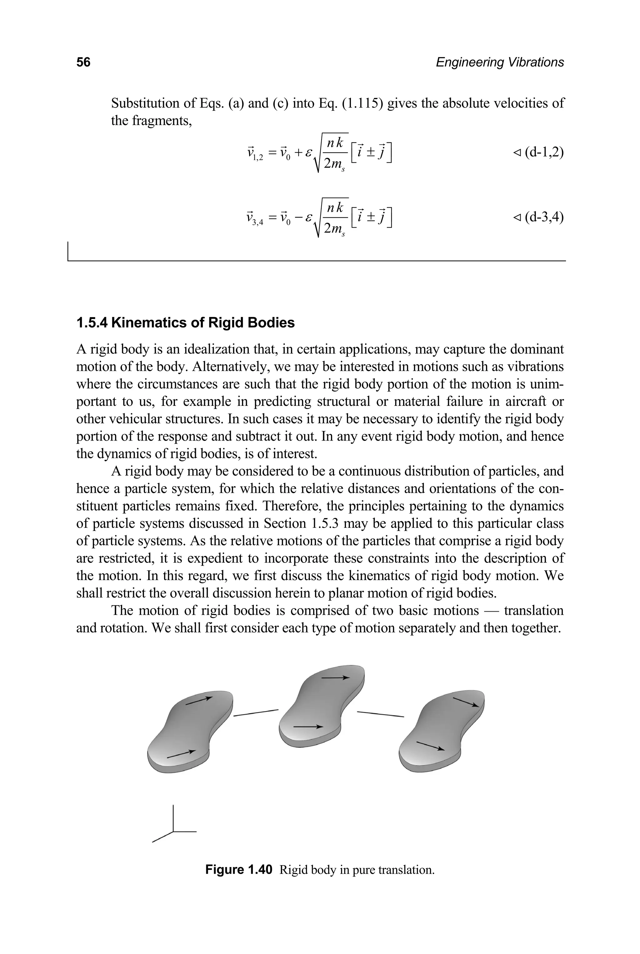
f a rigid body. For the special case of a rigid body with o
to translation, these equations reduce to Eq. (1.165).
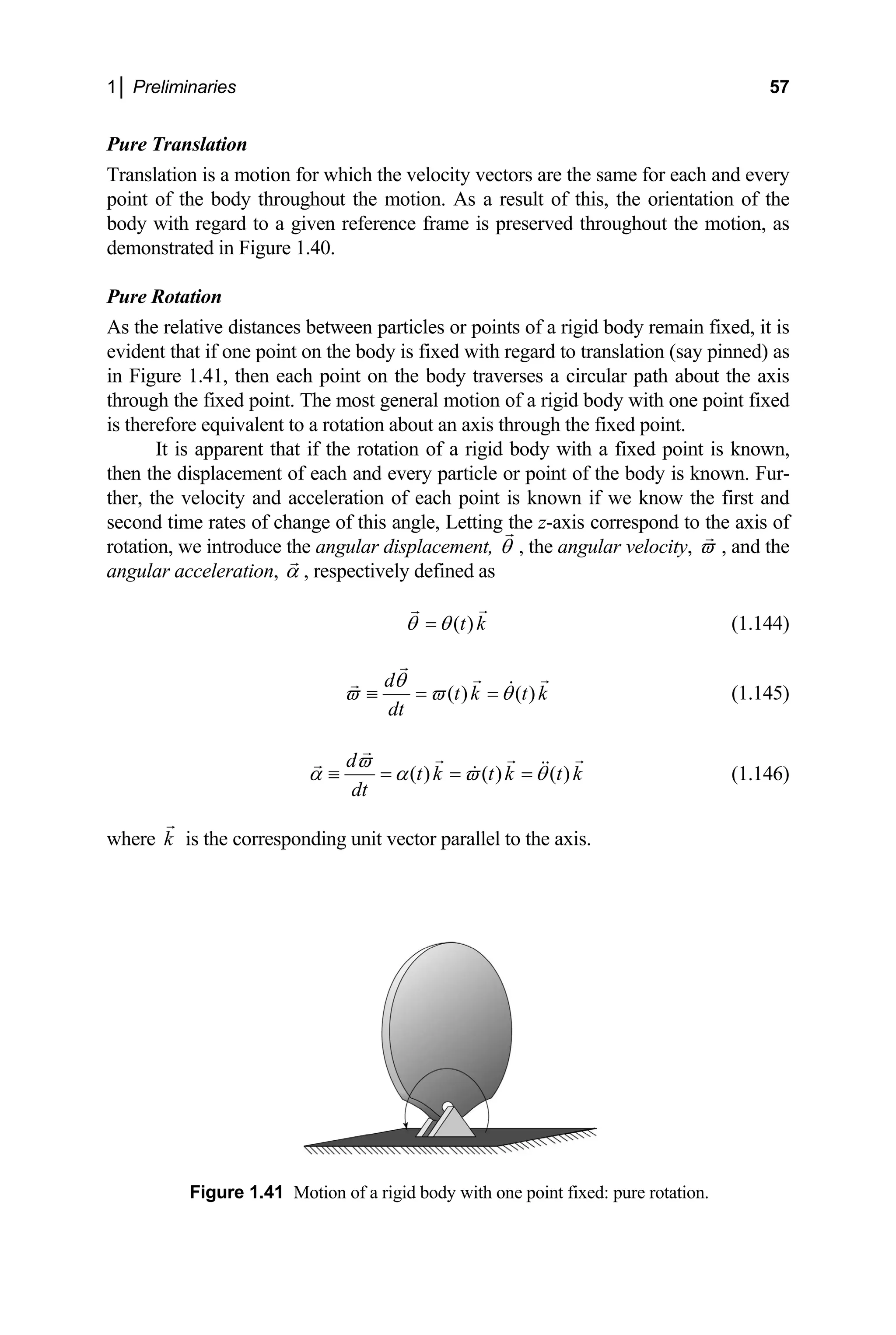
motion that were established above for a rigid body.
o ne point fixed with regard
Work and Energy
The relations that govern work and energy for a rigid body may be found by applying
the corresponding relations for particle systems in a manner similar to that which was
done to obtain the equations of motion. Alternatively, we can operate directly on the
equations of](https://image.slidesharecdn.com/engineeringvibrations-240713005818-b85f16c0/75/Engineering-Vibrations-Engineering-Vibrations-84-2048.jpg)
![66 Engineering Vibrations
( )
0
NC
O
M =
Application of Eq. (1.176) with gives
[ ]
2
1
2
0 0 ( / 2)cos
O
I mg L
θ
⎡ ⎤
= − + −
⎣ ⎦
on. Solving
for the angular speed, and using Eq. (1.78) and the relation IO = mL3
/3, gives
the speed of the tip of the rod as
0
θ − (a)
where we have chosen the datum to be at the horizontal configurati
0 0
tip θ θ
= =
directed to the left.
We next apply Eq. (1.165) and solve f
3
v L gL
θ
= = (b)
or α to get
2 0
0
( / 2)sin
0
O
mg L
I
θ
θ
θ
α α =
=
= = −
s. (b) and (c) and the
relation IO = mL /3, gives the reactions at the pin,
= (c)
Then, applying Eq. (1.160) in component form along the horizontal and vertical
directions when θ = 0, and incorporating the results of Eq
3
2
( / 2) 0
H
F m L α
= = (d-1)
2 3
2 2
( / 2)
V V 2.5
F mg m L F m g g
θ
− = ⇒ = + =
⎡ ⎤
⎣ ⎦ mg (d-2)
some fundamental issues pertinent to the
udy
eling
propr
of elementary dynamics. With this basic background we are now ready to begin our
study of vibrations. Additional background material will be introduced in subsequent
chapters, as needed.
1.6 CONCLUDING REMARKS
In this chapter we discussed and reviewed
st of vibrations. These included the concepts of degrees of freedom and the mod-
of complex systems as equivalent lower degree of freedom systems under ap-
iate circumstances. We also reviewed complex numbers and the basic principles](https://image.slidesharecdn.com/engineeringvibrations-240713005818-b85f16c0/75/Engineering-Vibrations-Engineering-Vibrations-88-2048.jpg)

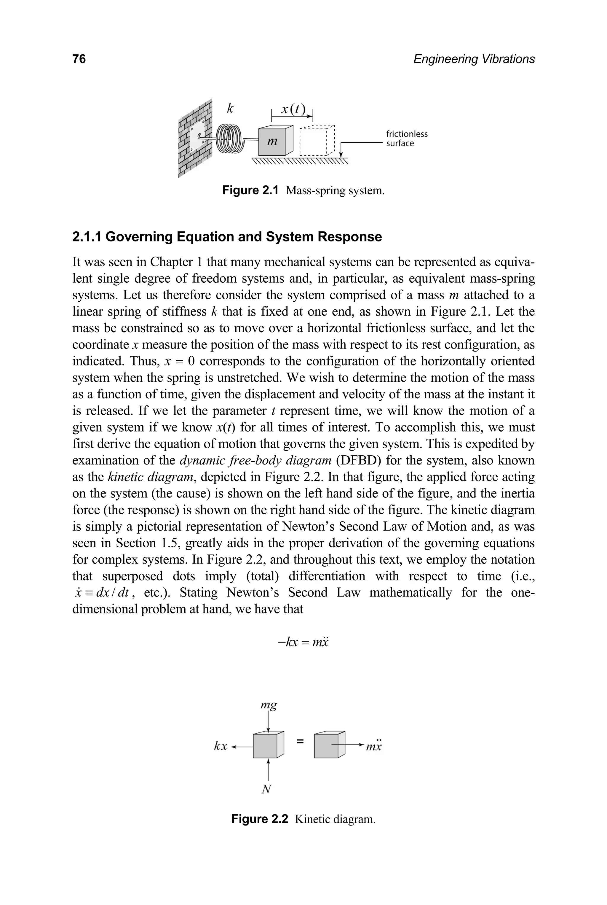
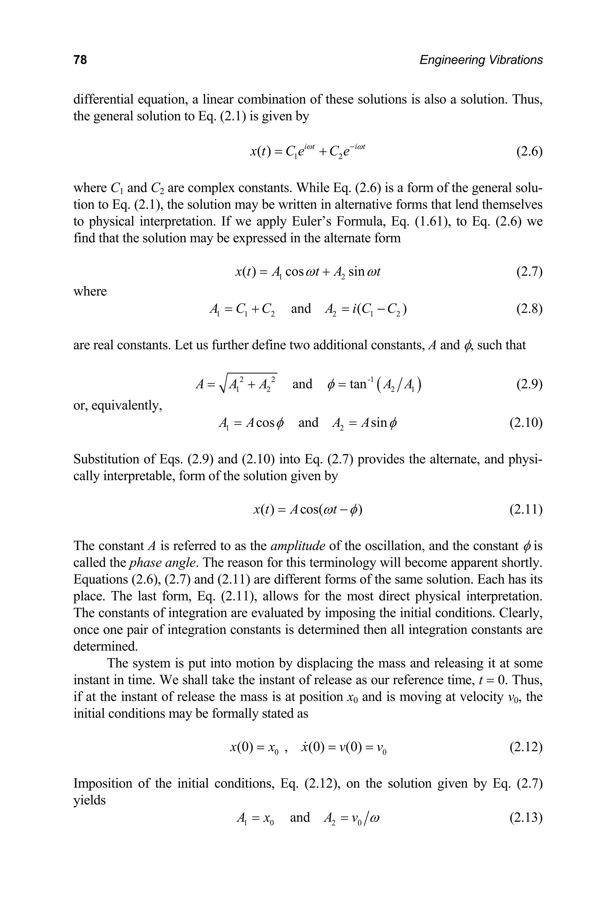
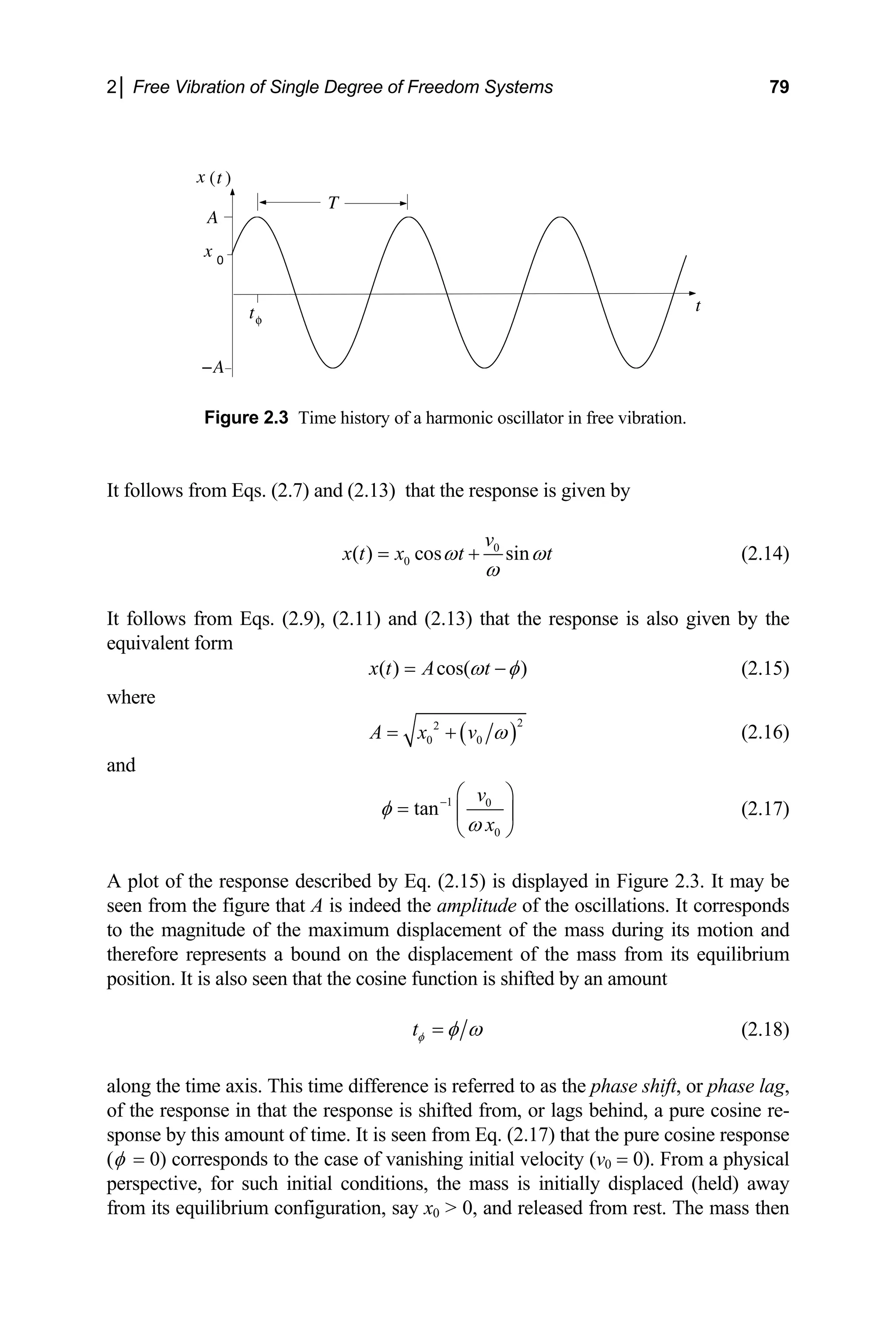
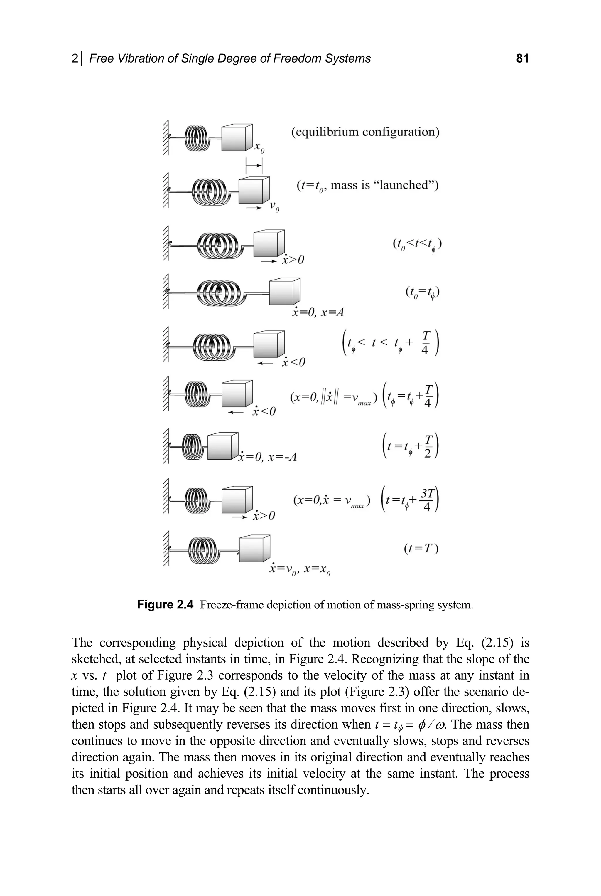
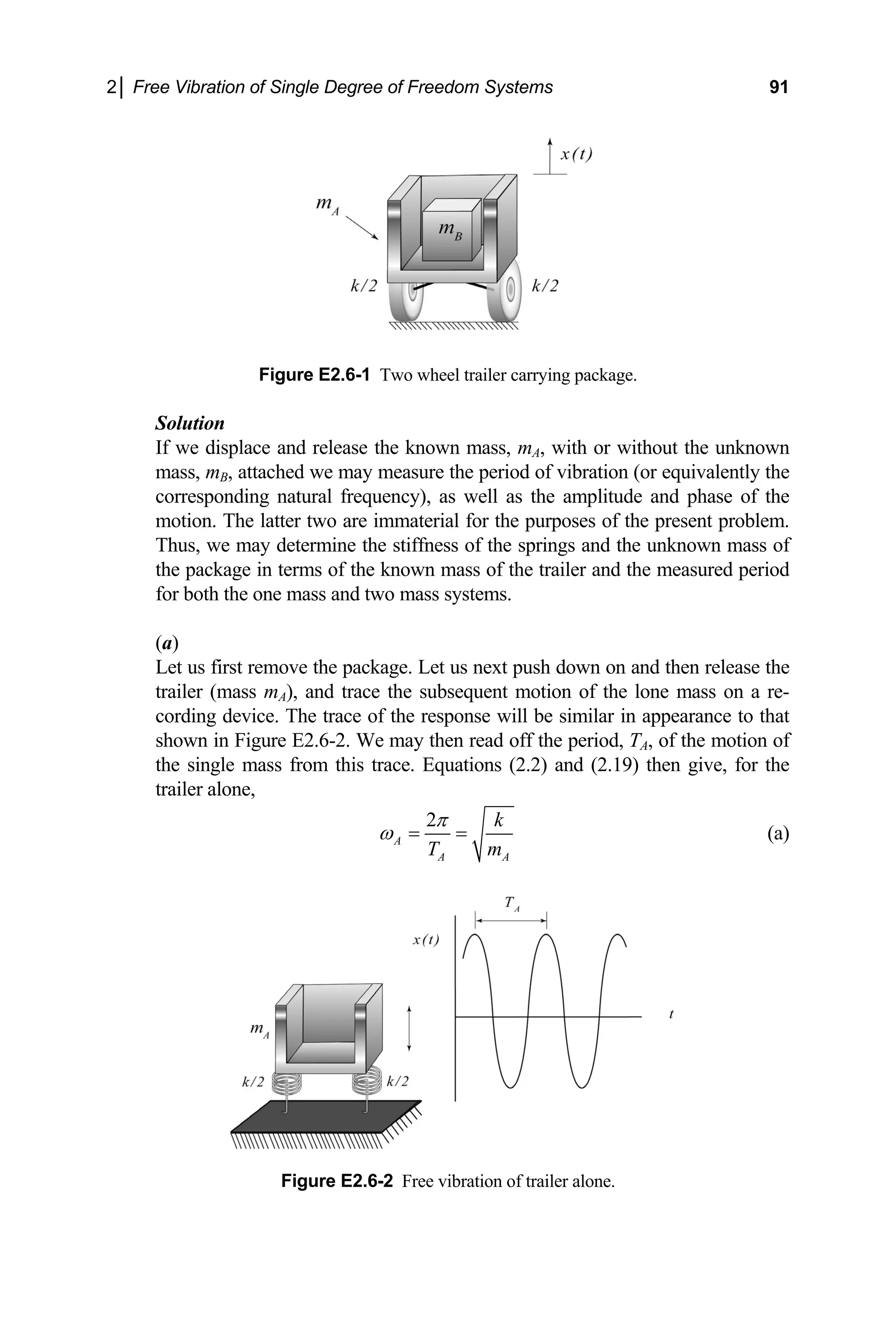
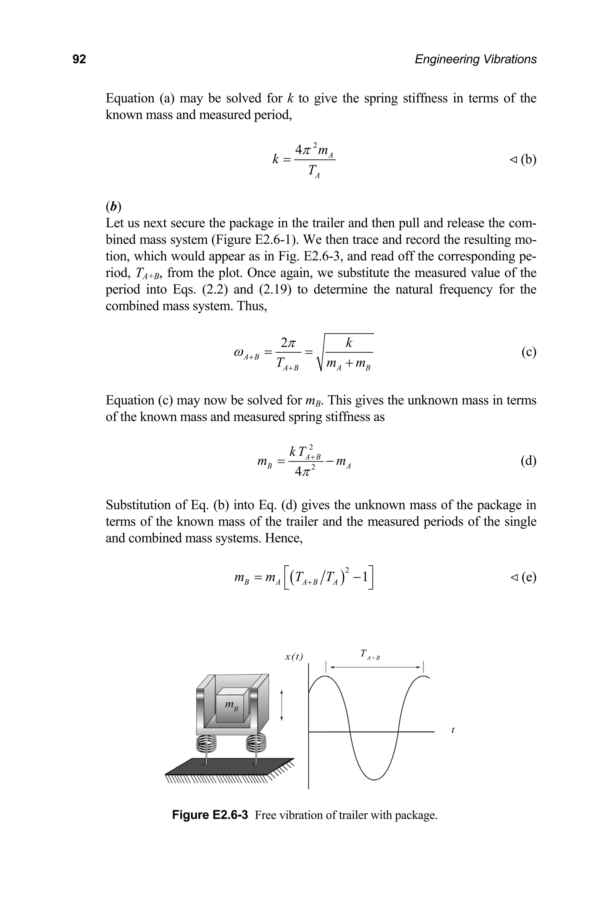
![2│ Free Vibration of Single Degree of Freedom Systems 77
Upon rearranging terms and dividing through by m, we obtain the governing equation
2
0
x x
ω
+ = (2.1)
where
k
m
ω = (2.2)
Equation (2.1) is known as the harmonic equation, and the parameter ω is referred to
as the natural (circular) frequency. It may be seen that the natural frequency defines
the undamped system in the sense that all the parameters that characterize the system
are contained in the single parameter ω. Thus, systems with the same stiffness to
mass ratio will respond in the same way to a given set of initial conditions. The
physical meaning and importance of the natural frequency of the system will be es-
tablished once we determine the response of the system. As the solution of Eq. (2.1)
will give the motion of the system as a function of time, we shall next determine this
solution.
Suppose the mass is pulled some distance away from its equilibrium position
and subsequently released with a given velocity. We wish to determine the motion of
the mass-spring system when it is released from such an initial configuration. That is,
we wish to obtain the solution to Eq. (2.1) subject to a general set of initial condi-
tions. To do this, let us assume a solution of the form
( ) st
x t Ce
∼ (2.3)
where e is the exponential function, and the parameters C and s are constants that are
yet to be determined. In order for Eq. (2.3) to be a solution to Eq. (2.1) it must, by
definition, satisfy that equation. That is it must yield zero when substituted into the
left-hand side of Eq. (2.1). Upon substitution of Eq. (2.3) into Eq. (2.1) we have that
( )
2 2
0
st
s Ce
ω
+ = (2.4)
Thus, for Eq. (2.3) to be a solution of Eq. (2.1), the parameters C and s must satisfy
Eq. (2.4). One obvious solution is C = 0, which gives ( ) 0
x t ≡ (the trivial solution).
This corresponds to the equilibrium configuration, where the mass does not move.
This solution is, of course, uninteresting to us as we are concerned with the dynamic
response of the system. For nontrivial solutions [ ( ) 0
x t ≠ identically], it is required
that . If this is so, then the bracketed term in Eq. (2.4) must vanish. Setting the
bracketed expression to zero and solving for s we obtain
0
C ≠
s iω
= ± (2.5)
where 1
i ≡ − . Equation (2.5) suggests two values of the parameter s, and hence two
solutions of the form of Eq. (2.3), that satisfy Eq. (2.1). Since Eq. (2.1) is a linear](https://image.slidesharecdn.com/engineeringvibrations-240713005818-b85f16c0/75/Engineering-Vibrations-Engineering-Vibrations-99-2048.jpg)
 (3 12)
64 8.43 10 psi
(0.1) (1)
G π
× ×
= = × (f)](https://image.slidesharecdn.com/engineeringvibrations-240713005818-b85f16c0/75/Engineering-Vibrations-Engineering-Vibrations-107-2048.jpg)
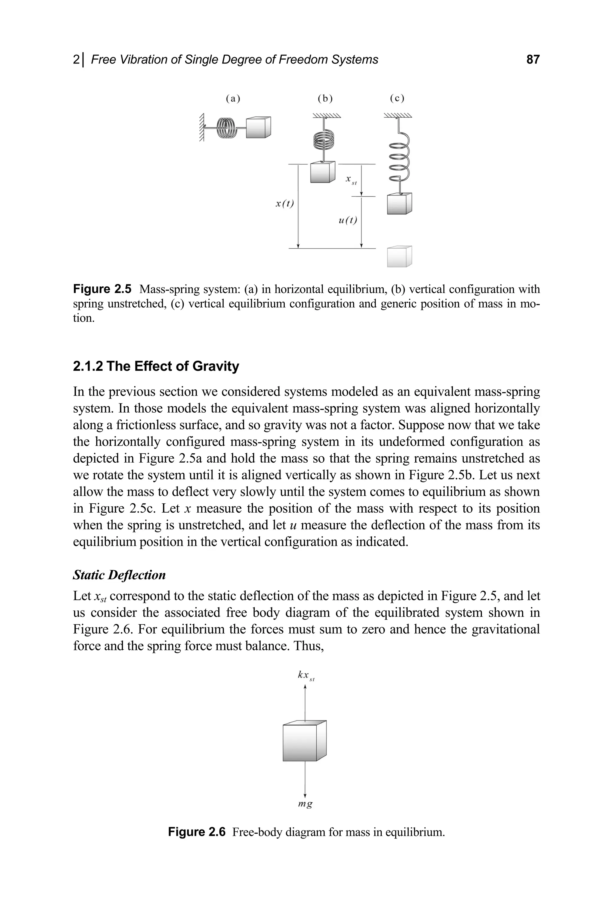
![86 Engineering Vibrations
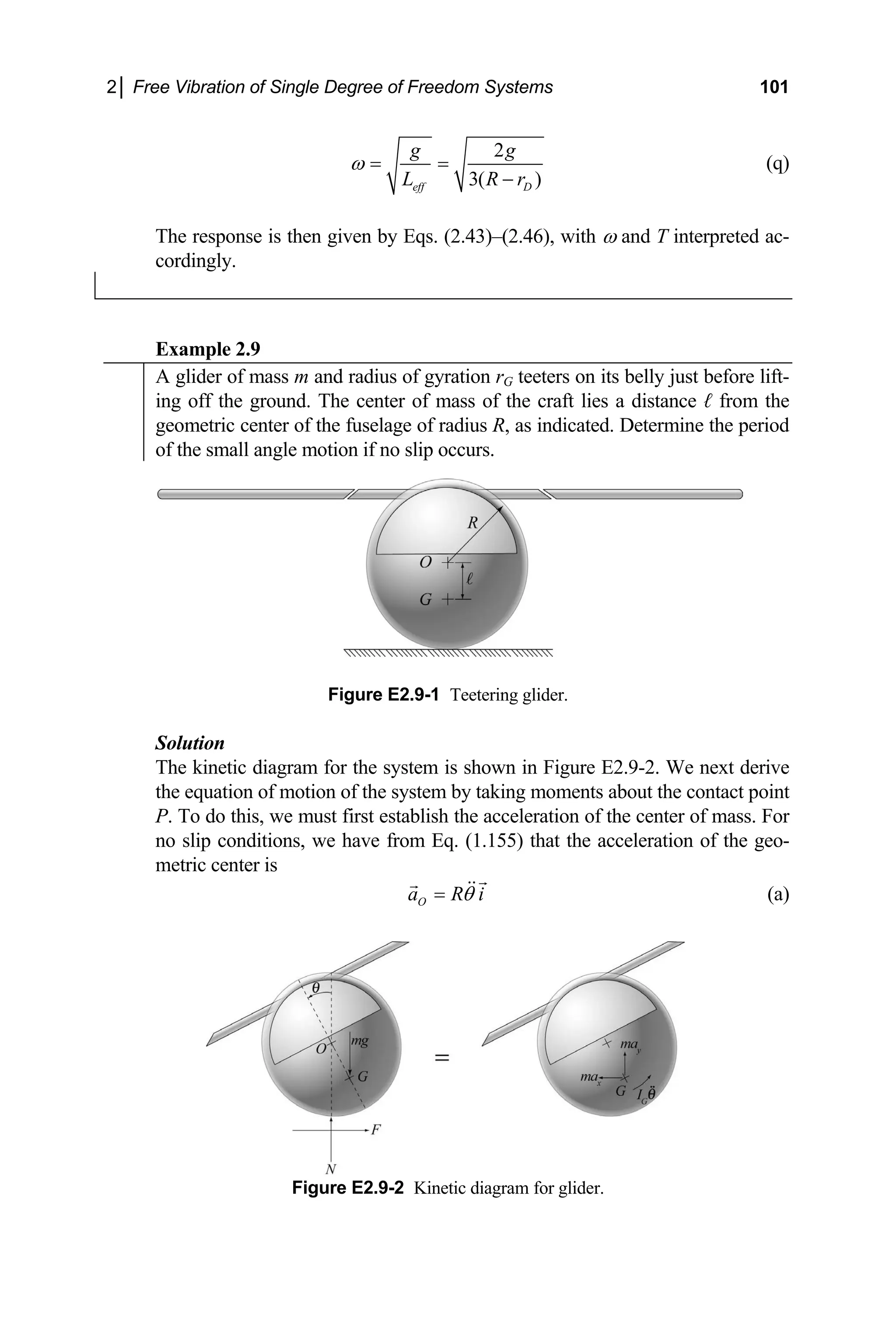
xample 2.4
E
A 200 lb man floats on a 6 ft by 2 ft inflatable raft in a quiescent swimming
pool. Estimate the period of vertical bobbing of the man and raft system should
the man be disturbed. Assume
that the weight of the man is
distributed uniformly over the
raft and that the mass of the raft
is negligible.
Solution
of the stiffness of the water, as pertains to the
e thus have from Eq. (1.40) that
The effect
man and the raft, is modeled as an equivalent spring as
discussed in Section 1.2.4. The corresponding equivalent
system is shown in the adjacent figure.
W
( ) 62.4[(2)(6)] 749 lb/ft
eq water
k g A
ρ
= = = (a)
he natural frequency of the system is then obtained from Eq. (2.2) as
T
749
11.0 rad/sec
200/32.2
ω = = (b)
quation (2.19) then gives the period as
E
2
0.571 sec
11.0
T
π
= = (c)
ow, from Table 2.1,
N
1
1.75 cps
0.571
ν = = (d)
hus, the man will oscillate through a little less than 2 cycles in a second. (How
T
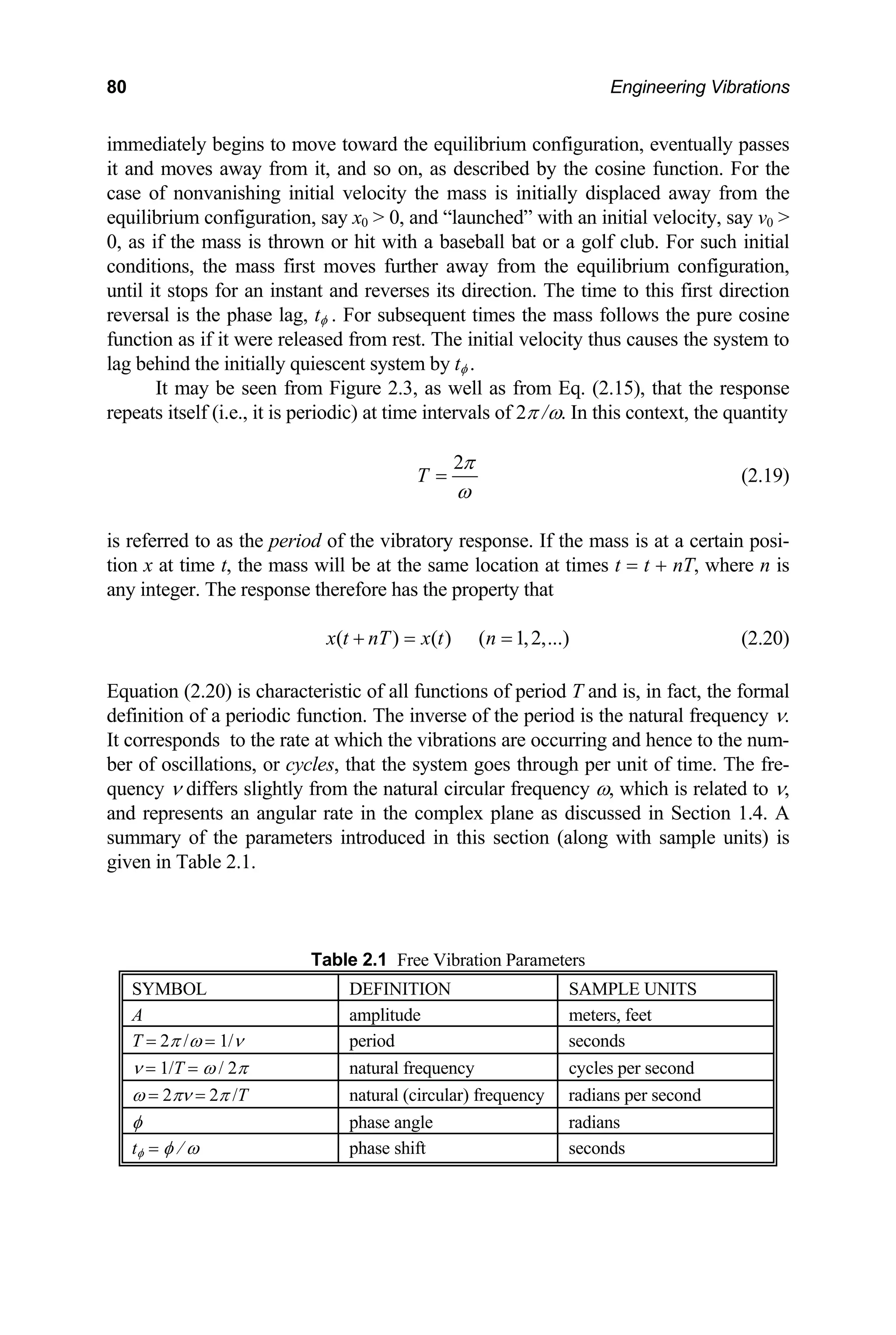
does this compare with your own experience?)](https://image.slidesharecdn.com/engineeringvibrations-240713005818-b85f16c0/75/Engineering-Vibrations-Engineering-Vibrations-108-2048.jpg)

![102 Engineering Vibrations
Figure E2.9-3 Relative motion of glider.
The acceleratio metric center is seen to
148) and (a), the accel-
eration of the center of
)
(b)
or small angle motion, let us linearize the above expression. Thus, neglecting
representation of the
cceleration of the center of mass as
n of the center of mass relative to the geo
be pure rotation (Figure E2.9-3). From Eqs. (1.72), (1.
mass with respect to the ground is
( ) (
/
2 2
sin cos cos sin
G O G O
a a a
R i i j
θ θ θ θ θ θ θ θ θ
= +
⎡ ⎤
= + − + +
⎣ ⎦
F
terms of second order and above gives the approximate
a
( )
G
a R i
θ
≅ − (c)
We next take moments about the contact point. Hence,
[ ]
/
sin G G P G z
mg I r ma
θ θ
− = + × (d)
inearizing the left hand side and substituting Eq. (c) gives the equation of mo-
L
tion as
2 2
( )
G
mg m r R
θ θ
⎡ ⎤
− = + −
⎣ ⎦ (e)
ringing nonvanishing terms to one side and dividing by the coefficient of
B
θ gives the equation of motion as
0
g
θ θ
eff
L
+ = (f)
where
2 2
( )
eff G
L r R
⎡ ⎤
= + −
⎣ ⎦ (g)](https://image.slidesharecdn.com/engineeringvibrations-240713005818-b85f16c0/75/Engineering-Vibrations-Engineering-Vibrations-124-2048.jpg)
![2│ Free Vibration of Single Degree of Freedom Systems 107
Let us next integrate Eq. (2.56) over the time interval [0, t] and divide the
resulting expression by the period of oscillation of the linear response,
0
2
T
g L
π
≡ (2.57)
Doing this gives the response as
( )
0
2
0
0
0
1
2
2 cos cos
t d
t
T
g L
θ
θ
θ
π χ
θ θ
≡ =
⎛ ⎞
− + ⎜ ⎟
⎝ ⎠
∫ (2.58)
where t is the normalized time. Equation (2.58) is the solution we are seeking
and may be integrated for given initial conditions to give the response.
Let us next consider motions for which the bob is released from rest
0
( 0)
χ = . In this way we exclude possible motions for which the bob orbits the
pin. We also know, from conservation of energy, that the motion is periodic.
Further, by virtue of the same arguments, we know that the time for the bob to
move between the positions θ = θ0 and θ = 0 is one quarter of a period. Like-
wise, the reverse motion, where the bob moves from the position θ = 0 to
θ = θ0, takes a quarter of a period to traverse as well. Taking this into account
and utilizing the equivalence of the cosine function in the first and fourth quad-
rants in Eq. (2.58) gives the exact period, T, of an oscillation of the simple pen-
dulum,
( )
0
0
0 0
1
4
2 2 cos cos
T d
T
T
θ
θ
π θ θ
≡ = ⋅
−
∫ (2.59)
where T is the normalized period. It is seen that the “true” period depends on
the initial conditions, that is 0
( )
T T θ
= , while the period predicted by the linear
approximation is independent of the initial conditions. We might expect, how-
ever, that the two solutions will converge as 0 0
θ → . It is left as an exercise
(Problem 2.24) to demonstrate that this is so. The integral of Eq. (2.59) may be
applied directly, or it may be put in a standard form by introducing the change
of variable
( )
1 1
sin sin 2
q
ϕ − ⎛ ⎞
≡ ⎜
⎝ ⎠
θ ⎟ (2.60)
where
( )
0
sin 2
q θ
≡ (2.61)
After making these substitutions, Eq. (2.59) takes the equivalent form](https://image.slidesharecdn.com/engineeringvibrations-240713005818-b85f16c0/75/Engineering-Vibrations-Engineering-Vibrations-129-2048.jpg)
![112 Engineering Vibrations
The terms within the brackets of Eq. (2.72) are seen to be identical in form to the
right-hand side of Eq. (2.6). It therefore follows from Eqs. (2.6)–(2.11) that the solu-
tion for the underdamped case (ζ 2
< 1) may also be expressed in the equivalent forms
[ ]
1 2
( ) cos sin
t
d d
x t e A t A t
ζω
ω ω
−
= + (2.73)
and
( ) cos( ) ( )cos( )
t
d d d
x t Ae t A t t
ζω
ω φ ω
−
= − = φ
− (2.74)
where
( ) t
d
A t Ae ζω
−
= (2.75)
and the pairs of constants (A, φ), (A1, A2) and (C1, C2) are related by Eqs. (2.8), (2.9)
and (2.10). The specific values of these constants are determined by imposing the
initial conditions
0 0
(0) and (0)
x x x v
= =
on the above solutions. Doing this gives the relations
( )
0
1 0 2
2
,
1
v
A x A
0
x
ω ζ
ζ
+
= =
−
(2.76)
and
( ) ( )
2
0 0 0 0
1
0 2 2
1 , tan
1 1
v x v x
A x
ω ζ ω ζ
φ
ζ ζ
−
⎛ ⎞
+
⎡ ⎤ +
⎣ ⎦ ⎜
= + =
⎜
− −
⎝ ⎠
⎟
⎟
(2.77)
It may be seen from Eqs. (2.74) and (2.75) that the response of the system corre-
sponds to harmonic oscillations whose amplitudes, Ad(t), decay with time at the rate
ζω (= c/2m). It may be noted that the frequency of the oscillation for the under-
damped case is ωd, as defined by Eq. (2.70). It follows that the corresponding period
is
2
2 2
1
d
d
T
π π
ω ω ζ
= =
−
(2.78)
and that the associated phase lag is
d
tφ ω φ
= (2.79)
Note that the frequency of the damped oscillations is lower, and hence the corre-
sponding period is longer, than that for the undamped system (ζ = 0). It is thus seen
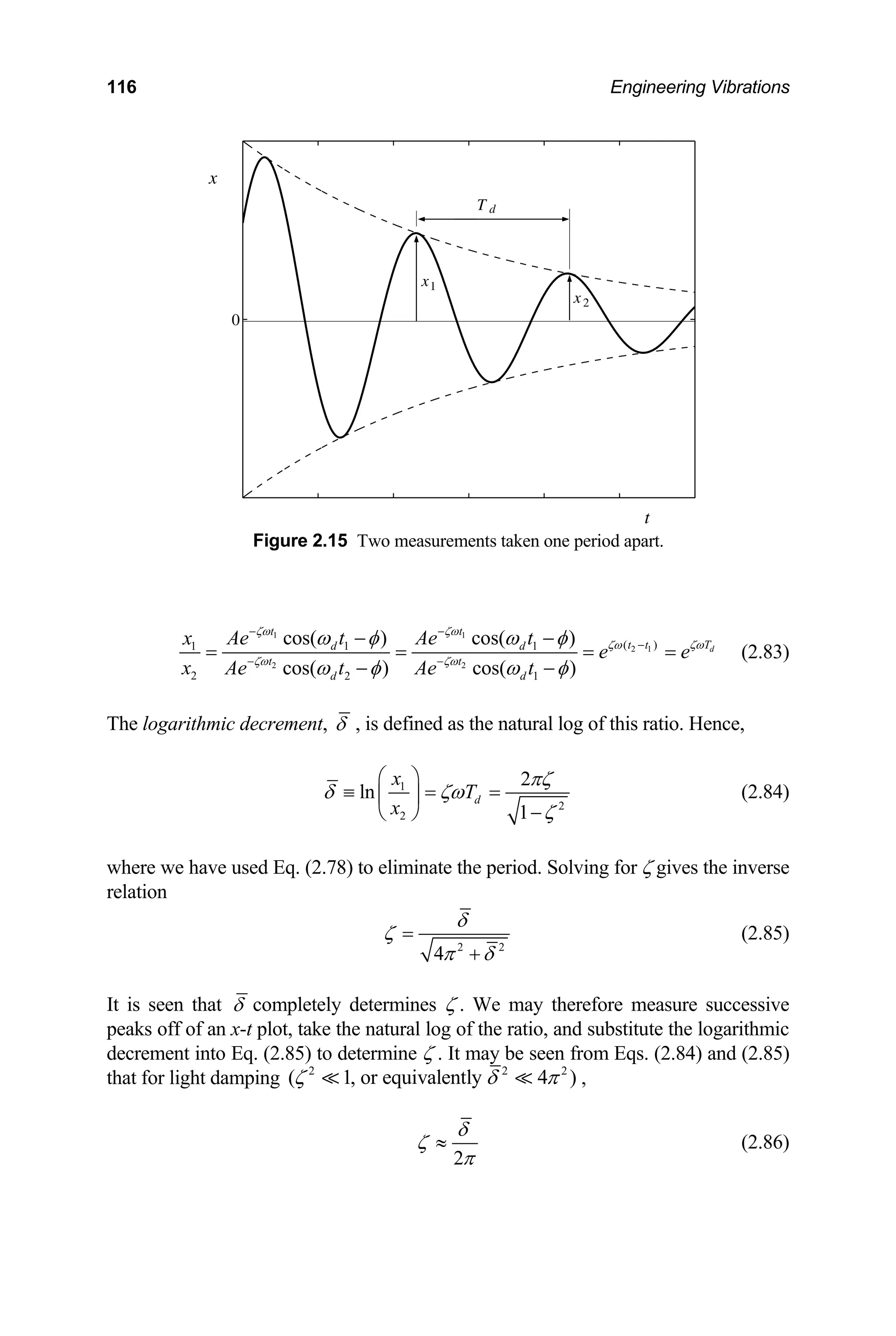
that damping tends to slow the system down, as might be anticipated.](https://image.slidesharecdn.com/engineeringvibrations-240713005818-b85f16c0/75/Engineering-Vibrations-Engineering-Vibrations-134-2048.jpg)
![2│ Free Vibration of Single Degree of Freedom Systems 119
We next employ Eq. (2.90) where, for the present problem, n = 3 and x1 = 0.5
m. This gives the desired position directly as
(d-1)
3(0.2)(10)(0.6413)
(3 ) 0.5 0.01066 m
d
x T e−
= =
Equivalently,
2
6 (0.2) 1 (0.2)
(3 ) 0.5 0.01066 m
d
x T e π
− −
= = (d-2)
2.2.4 Overdamped Systems 2
( 1
ζ > )
t
Systems for which ζ 2
> 1 are referred to as overdamped systems. For such systems,
the characteristic roots given by Eq. (2.68) are all real. Substitution of these roots into
Eq. (2.66) gives the solution for the overdamped case as
( ) ( )
1 2
( ) t
x t C e C e
ζ ω ζ ω
− − − +
= +
z z
(2.91)
where
2
1
ζ
= −
z (2.92)
An equivalent form of the solution is easily obtained with the aid of Eq. (1.63) as
[ ]
1 2
( ) cosh sinh
t
x t e A t A t
ζω
ω ω
−
= +
z z
2
(2.93)
and
1 1 2 2 1
,
A C C A C C
= + = − (2.94)
Upon imposing the initial conditions 0
(0)
x x
= and 0
(0)
x v
= , Eq. (2.93) gives the
integration constants as
( )
0
1 0 2
2
,
1
v x
A x A 0
ω ζ
ζ
+
= =
−
(2.95)
The solution for the overdamped case then takes the form
( )
0 0
0
( ) cosh sinh
t v x
x t e x t t
ζω ζω
ω ω
ω
− +
⎡ ⎤
= +
⎢ ⎥
⎣ ⎦
z
z
z (2.96)
where z is given by Eq. (2.92). Consideration of the exponential form of the solution,
Eq. (2.91), shows that both terms of the solution decay exponentially. A typical re-
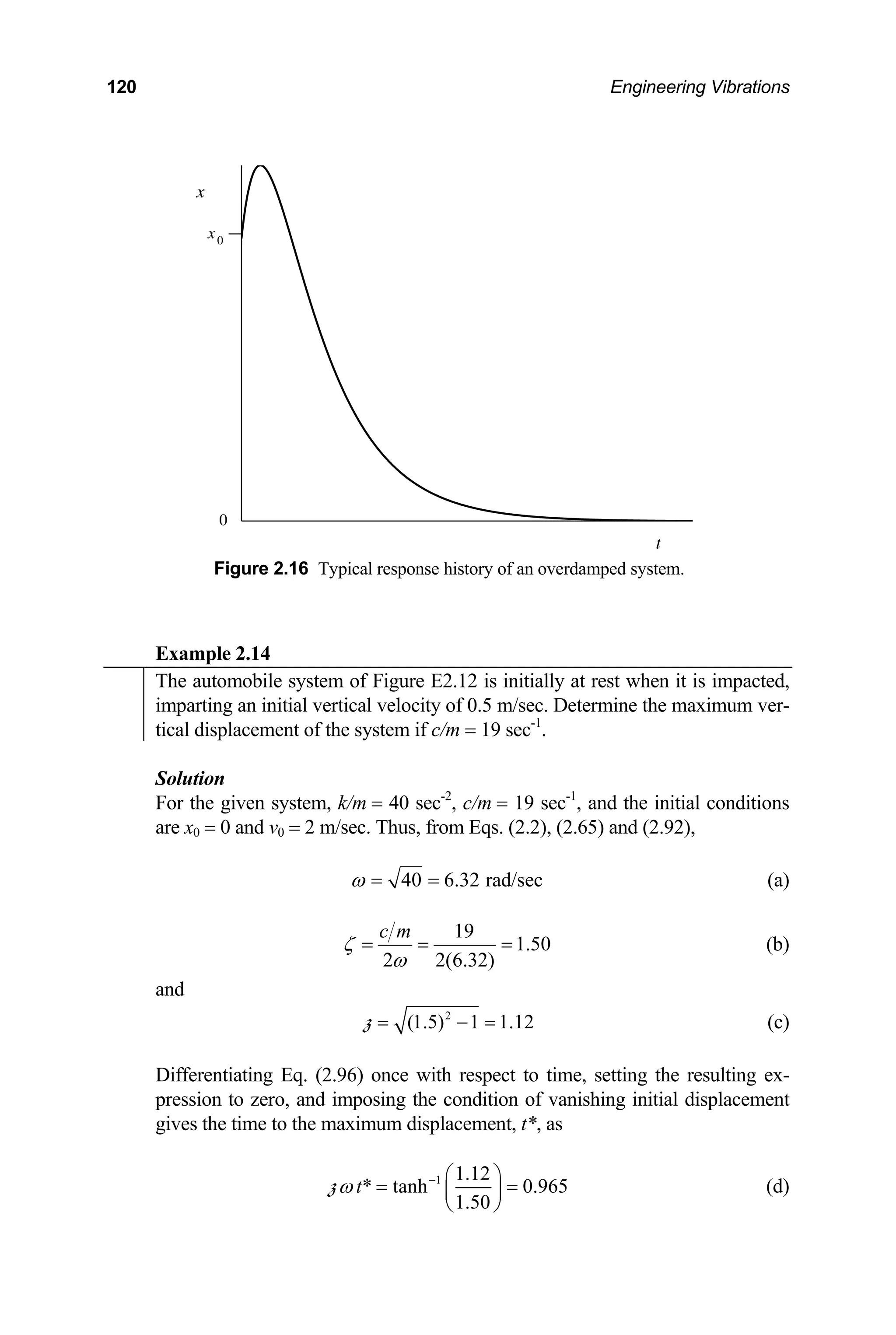
sponse is depicted in Figure 2.16.](https://image.slidesharecdn.com/engineeringvibrations-240713005818-b85f16c0/75/Engineering-Vibrations-Engineering-Vibrations-141-2048.jpg)
![2│ Free Vibration of Single Degree of Freedom Systems 121
Hence,
* 0.641 [(1.12)(6.32)] 0.136 secs
t = = (e)
Substitution of the nondimensional time, Eq. (d), or the dimensional time, Eq.
(e), into Eq. (2.96) gives the maximum deflection. Thus,
*
0
max
1.50(0.136)
( *) sinh( *)
0.5
sinh(0.965)
(6.32)(1.12)
0.0647 m 6.47 cm
t
v
x x t e t
e
ζω
ω
ω
−
−
= =
=
= =
z
z
(f)
2.2.5 Critically Damped Systems 2
( 1
ζ )
=
It was seen in the prior two sections that the response of an underdamped system (ζ 2
< 1) is a decaying oscillation, while the response of an overdamped system (ζ2
> 1) is
an exponential decay with no oscillatory behavior at all. A system for which ζ 2
=1 is
referred to as critically damped since it lies at the boundary between the under-
damped and overdamped cases and therefore separates oscillatory behavior from
nonoscillatory behavior. We examine this case next.
For critically damped systems, the characteristic roots given by Eq. (2.68) re-
duce to
,
s ω ω
= − − (2.97)
When substituted into Eq. (2.66), these roots yield the solution for the critically
damped case in the form
( )
1 2
( ) t
x t A A t e ω
−
= + (2.98)
where the factor t occurs because the roots are repeated. Imposition of the initial con-
ditions, 0
(0)
x x
= and 0
(0)
x v
= , renders the response given by Eq. (2.98) to the
form
( )
0 0 0
( ) t
x t x v x t e ω
ω −
= + +
⎡ ⎤
⎣ ⎦ (2.99)
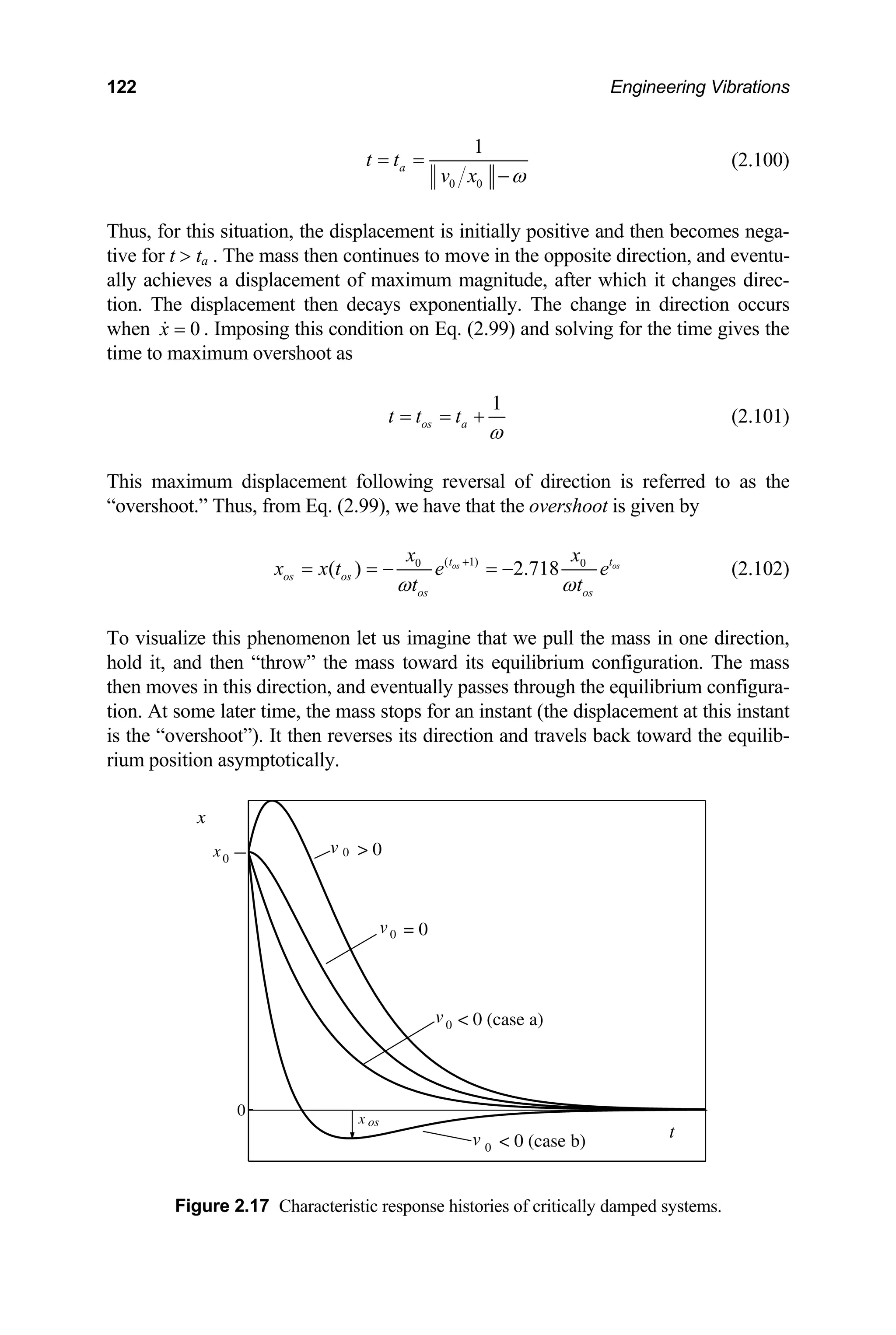
ial velocity
Representative characteristic responses are displayed in Figure 2.17. It is seen from
Eq. (2.99) that when the initial displacement and the init are of opposite
sign and the latter is of sufficient magnitude, such that 0 0 1
v x
ω < − , then the dis-
lacement passes through zero once and occurs at time
p](https://image.slidesharecdn.com/engineeringvibrations-240713005818-b85f16c0/75/Engineering-Vibrations-Engineering-Vibrations-143-2048.jpg)
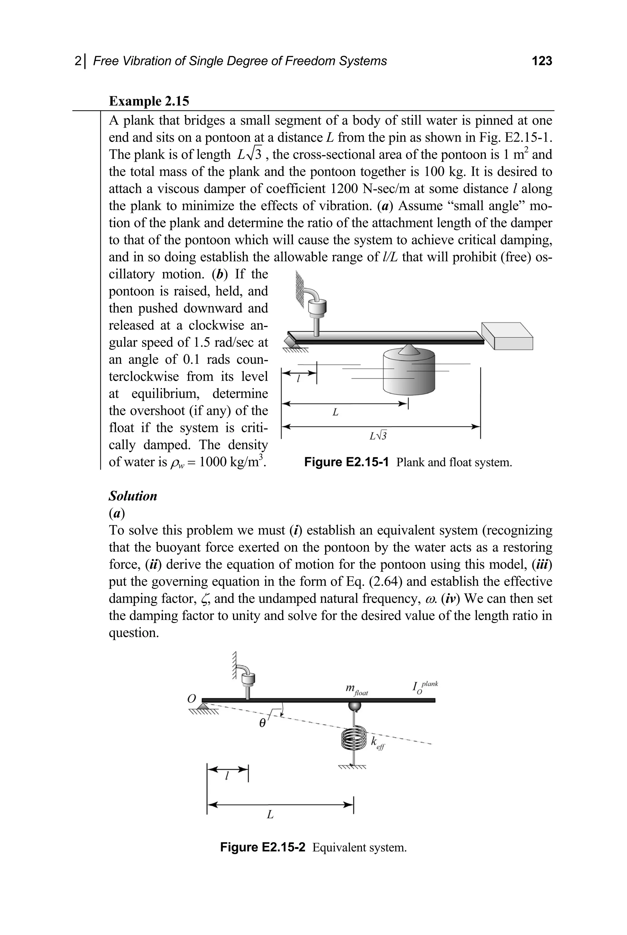
![124 Engineering Vibrations
(i) The equi , using Eq. (1.40),
Figure E2.15-3 Kinetic diagram.
valent system is shown in Figure E2.15-2 where
(1000)(9.81)(1) 9810 N
eff w
k gA /m
ρ
= = = (a)
e
(ii) To derive the governing equation of motion for the equivalent system we
first draw the kinetic diagram shown in Fig. E2.15-3. As we need the rotational
acceleration of the plank and the velocity of the damper, as well as the dis-
placement of the mass, it is convenient to express our equations in terms of th
angular coordinate ( )
t
θ .
The damping force, Fd, and the spring force, Fs, are respectively
d l
F cs clθ
= = (b)
and
sin
s eff L eff
F k y k L θ
= = (c)
he inertia force of the pontoon may be resolved into its normal and tangential
T
components, fl n
m a and fl t
m a , with regard to the circular path described by the
float, where an and at are respectively the normal and tangential components of
the acceleration of the pontoon, and mfl is its mass. Thus, if s = Lθ is the path
coordinate for the pontoon, we have from Eq. (1.76) that
2
2
s
m a m m L
fl n fl fl
L
θ
= = (d)
L
fl t fl fl
m a m s m θ
= =
[Note that we could have just as easily used pol
= L.] The moment of inertia of the plank about hinge O is given by
(e)
ar coordinates, Eq. (1.79), with
R
( ) 2
1
3
pl
O pl pl
I m L
= (f)
where mpl and Lpl respectively correspond to the mass and length of the plank,
nd we have modeled the plank as a (uniform) rod. For th
a
le
e present problem the
ngth of the plank is given as](https://image.slidesharecdn.com/engineeringvibrations-240713005818-b85f16c0/75/Engineering-Vibrations-Engineering-Vibrations-146-2048.jpg)
![126 Engineering Vibrations
(iv) For critical damping, we set ζ = 1 in Eq. (m) and so itical
length ratio. Doing this gives
lve for the cr
1/ 2
2 2(9.90)(100)
1.28
= (n)
1200
cr
l m
L c
ω
⎛ ⎞ ⎡ ⎤
= =
⎜ ⎟ ⎢ ⎥
⎝ ⎠ ⎣ ⎦
Thus, for the system to avoid free vibratory behavior, the length rat
such that
io must be
1/ 2
2
1.28
l mk
L c
⎡ ⎤
≥ =
⎢ ⎥
⎣ ⎦
(o)
(b) Let us first check to see that there will be an overshoot. Hence,
0 0 1.5 [9.9( 0.1)] 16.67 1
v ωθ = − = − < −
Since the ratio satisfies the requisite inequality, we anticipate that the plank will
pass through its equilibrium position one time before retu
cally. We now proceed to calculate by how much. To deter
e first calculate the time to the overshoot. Substitution of the given initial
.100) gives the time to crossing the equilibrium position as
rning to it asymptoti-
mine the overshoot,
w
conditions and the value of the undamped natural frequency given by Eq. (l)
into Eq. (2
1
0.196 secs
(1.5)/( 0.1) 9.9
a
t = =
− −
(p)
me to over-
oot as
ubstitution of Eqs. (l) and (p) into Eq. (2.101) then gives the ti
S
sh
1
0.196 0.297 secs
9.90
os
The overshoot may now be determined using Eq. (2.102). Thus,
t = + = (q)
0.297
( 0.10)
2.718 0.0458 rads
(9.90)(0.297)
os e
θ
−
= − = (r)](https://image.slidesharecdn.com/engineeringvibrations-240713005818-b85f16c0/75/Engineering-Vibrations-Engineering-Vibrations-148-2048.jpg)
![148 Engineering Vibrations
0 0
ˆ( ) cos sin i t
0
F t F t iF t F e Ω
= Ω + Ω = (3.12)
It follows from Eqs. (3.8)–(3.10) that once the response to the complex force is de-
termined then the response to the cosine function will be the real part of the complex
response and the response to the sine function will be the imaginary part of the com-
plex response. We shall therefore solve the problem
2 2 2
0
ˆ
ˆ ˆ ˆ
2 ( ) i t
x x x f t f e
ωζ ω ω ω Ω
+ + = =
(3.13)
where
0 0
f F k
= (3.14)
It may be seen that the parameter f0 corresponds to the deflection that the mass of the
system would undergo if it was subjected to a static force of the same magnitude, F0,
as that of the dynamic load.
The general solution of Eq. (3.13) consists of the sum of the complementary
solution and the particular solution associated with the specific form of the forcing
function considered. Hence,
ˆ ˆ ˆ
( ) ( ) ( )
c p
x t x t x t
= + (3.15)
where subscripts c and p indicate the complementary and particular solution, respec-
tively. The former corresponds to the solution to the associated homogeneous equa-
tion, as discussed in Chapter 2. Incorporating Eqs. (2.11), (2.74), (2.93) and (2.98)
gives the general solutions for undamped and viscously damped systems as
(3.16)
( ) cos( ) ( ) (0 1)
t
d p
x t Ae t x t
ζω
ω φ ζ
−
= − + ≤
[ ]
1 2
( ) cosh sinh ( ) ( 1)
t
p
x t e A t A t x t
ζω
ω ω ζ
−
= + +
z z (3.17)
( )
1 2
( ) ( ) ( 1)
t
p
x t A A t e x t
ω
ζ
−
= + + = (3.18)
where ωd and z are defined by Eqs. (2.70) and (2.92), respectively. The constants of
integration are evaluated by imposition of the initial conditions on the pertinent form
of the response, Eq. (3.16), (3.17) or (3.18), after the specific form of the particular
solution is determined.
It is seen that the complementary solution damps out and becomes negligible
with respect to the particular solution after a sufficient amount of time. (Note that the
undamped case, ζ = 0, is an idealization for very light damping. Since all systems
possess some damping we shall, for the purposes of the present discussion, consider
the complementary solution to decay for vanishing damping as well.) Since we are
presently considering forces that act continuously over very long time intervals, the
particular solution for these cases corresponds to the steady state response of the sys-](https://image.slidesharecdn.com/engineeringvibrations-240713005818-b85f16c0/75/Engineering-Vibrations-Engineering-Vibrations-170-2048.jpg)
![150 Engineering Vibrations
( )
0 2
1
1
Γ Ω =
− Ω
(3.24)
and
0 when 1
when 1
π
Φ = Ω
Φ = Ω
(3.25)
Substituting Eq. (3.20) into Eq. (3.19) and using Euler’s Formula gives the particular
solution
[ ] [ ]
0
2
ˆ ( ) cos( ) sin( ) cos sin
1
ss
f
x t X t i t t i t
= Ω − Φ + Ω − Φ = Ω + Ω
− Ω
(3.26)
As discussed at the end of Section 3.2, the response to the real part of a complex forc-
ing function is the real part of the complex response. Likewise, the response to the
imaginary part of a complex forcing function is the imaginary part of the complex
response. Thus, pairing Eq. (3.26) with Eq. (3.12) in this sense, we find the following
responses:
if 0
( ) cos
F t F
= t
Ω , then
0
2
( ) cos( ) cos
1
ss
f
x t X t t
= Ω − Φ = Ω
− Ω
(3.27)
if 0
( ) sin
F t F t
= Ω , then
0
2
( ) sin( ) sin
1
ss
f
x t X t t
= Ω − Φ = Ω
− Ω
(3.28)
0
f(t)
x(t)
t
t
f
0
−f0
0
0
f
−f
0
0
Figure 3.3 Typical time histories of excitation, and response,
( ),
f t ( ),
x t for 1.
Ω](https://image.slidesharecdn.com/engineeringvibrations-240713005818-b85f16c0/75/Engineering-Vibrations-Engineering-Vibrations-172-2048.jpg)
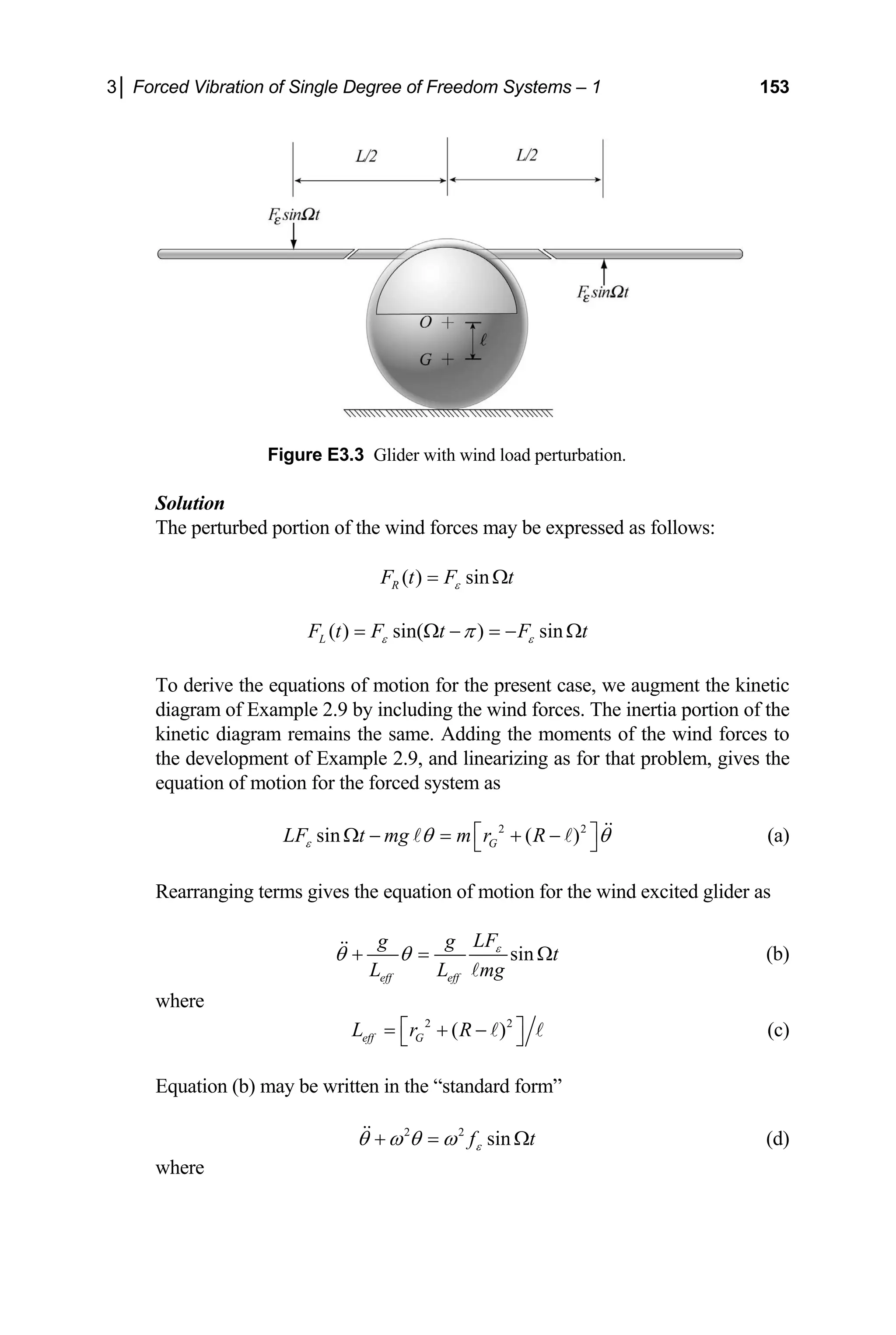
![3│ Forced Vibration of Single Degree of Freedom Systems – 1 155
1
0
2
Ĉ i f
ω
= − (3.31)
Substituting Eq. (3.31) back into Eq. (3.30) and using Euler’s Formula gives the par-
ticular solution of Eq. (3.29) as
or
[ ]
[ ]
1
0
2
1
0
2
( ) sin cos
( ) cos( / 2) sin( / 2)
ss
ss
x t f t t i t
x t f t t i t
ω ω ω
ω ω π ω π
= −
= − + −
(3.32)
As per earlier discussions, the real part of the solution is the response to the real part
of the complex forcing function, and the imaginary part of the solution is the response
to the imaginary part of the complex forcing function. Thus,
when 0
( ) cos ,
F t F t
ω
=
1
0
2
( ) sin ( )cos( / 2)
ss
x t f t t X t t
ω ω ω π
= = − (3.33)
when 0
( ) sin ,
F t F t
ω
=
1
0
2
( ) cos ( )sin( / 2)
ss
x t f t t X t t
ω ω ω π
= − = − (3.34)
where
1
0
2
( )
X X t f t
ω
= = (3.35)
is the (time dependent) amplitude of the steady state response. It is seen that, when
the forcing frequency is numerically equal to the natural frequency of the undamped
system, the steady state response of the system is out of phase with the force by
Φ = π/2 radians and hence lags the force by tlag = π /2ω. The amplitude, X, is seen to
grow linearly with time. A typical response is displayed in Figure 3.4. We see that,
when the undamped system is excited by a harmonically varying force whose fre-
quency is identical in value to the natural frequency of the system, the steady state
response increases linearly in time without bound. This phenomenon is called reso-
nance. Clearly the energy supplied by the applied force is being used in an optimum
manner in this case. We certainly know, from our discussions of free vibrations in
Chapter 2, that the system moves naturally at this rate (the natural frequency) when
disturbed and then left on its own. The system is now being forced at this very same
rate. Let’s examine what is taking place more closely.
To better understand the mechanics of resonance let us examine the work done
by the applied force over one cycle of motion, nT t (n + 1)T, where T is the period
of the excitation (and thus of the steady state response as well) and n is any integer.
We shall compare the work done by the applied force, F(t), for three cases; (i) 1,
Ω
(ii) 1
Ω and (iii) 1
Ω = .](https://image.slidesharecdn.com/engineeringvibrations-240713005818-b85f16c0/75/Engineering-Vibrations-Engineering-Vibrations-177-2048.jpg)
![156 Engineering Vibrations
0
x(t)
t
Figure 3.4 Time history of the response of a system at resonance.
From the definition of work given in Section 1.5.2 [see Eqs. (1.85) and (1.87)],
and utilization of the chain rule of differentiation, the work done by the applied force
for the single degree of freedom system under consideration is seen to be given by the
relation
2 2
1 1
x t
x t
Fdx Fx dt
= =
∫ ∫
W (3.36)
where x1 = x(t1), x2 = x(t2) and, for the interval under consideration, t1 = nT and T2
= (n + 1)T for any given n.
For the sake of the present discussion we will assume, without loss of general-
ity, that the forcing function is of the form of a cosine function. The response is then
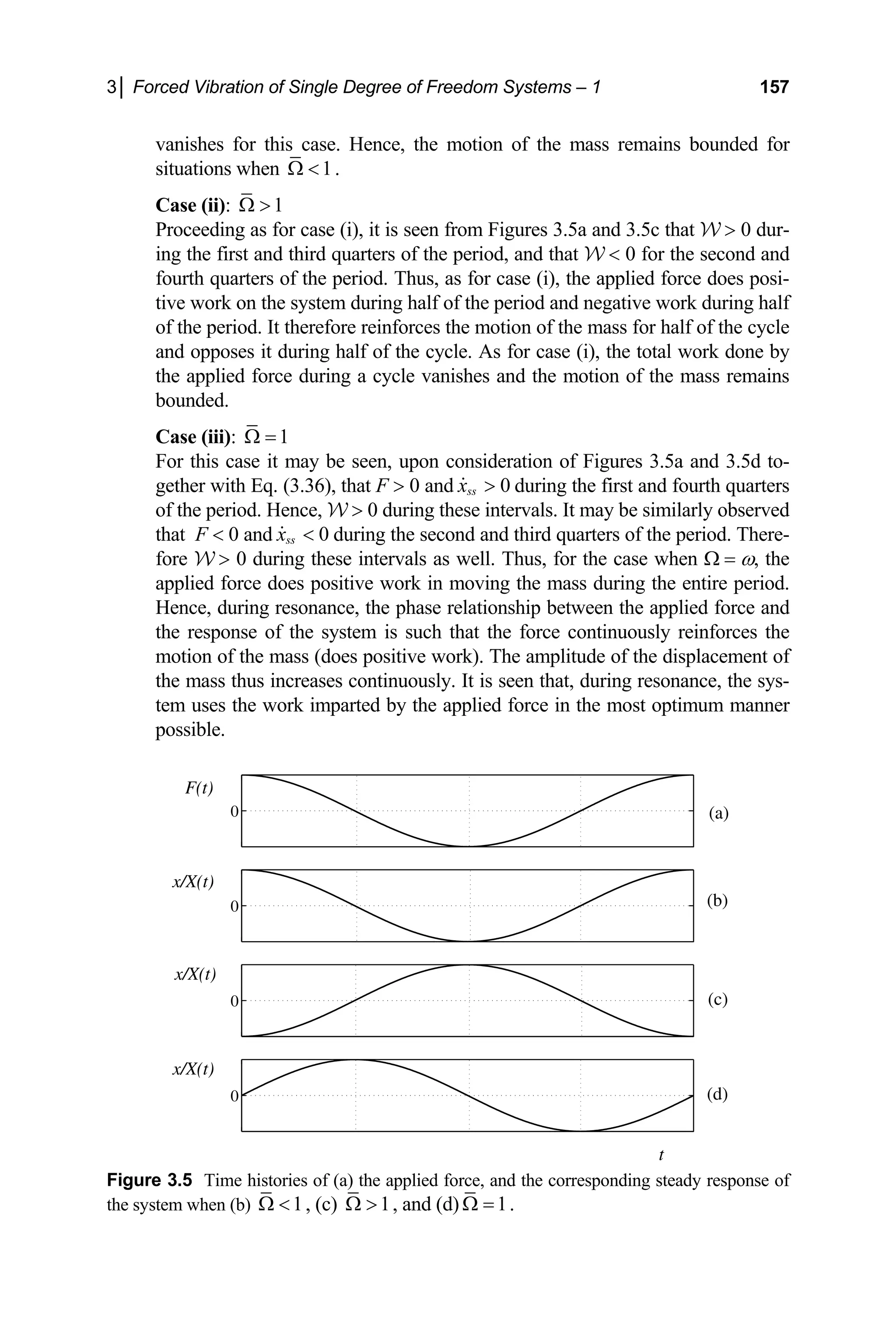
given by Eq. (3.33). Typical plots of the applied force and the resulting steady state
response for cases (i)–(iii) are displayed as functions of time over one cycle in Fig-
ures 3.5a–3.5d, respectively. Noting that the slope of the response plot corresponds to
the velocity of the mass, we can examine the work done by the applied force qualita-
tively during each quarter of the representative period considered for each case.
Case (i): 1
Ω
Consideration of Figures 3.5a and 3.5b shows that F 0 and 0
ss
x
in the first
quadrant. Thus, it may be concluded from Eq. (3.36) that W 0 over the first
quarter of the period. If we examine the second quadrant, it is seen that F 0
and during this interval. Hence, W 0 during the second quarter of the
period. Proceeding in a similar manner, it is seen that F 0 and during
the third quarter of the period. Hence, W 0 during this interval. Finally, it
may be observed that F 0 and during the fourth quarter of the period.
Therefore, W 0 during the last interval. It is thus seen that the applied force
does positive work on the system during half of the period and negative work
during half of the period. Therefore, the applied force reinforces the motion of
the mass during half of the period and opposes the motion of the mass during
half the period. In fact, the total work done by the applied force over a cycle
0
ss
x
0
ss
x
0
ss
x](https://image.slidesharecdn.com/engineeringvibrations-240713005818-b85f16c0/75/Engineering-Vibrations-Engineering-Vibrations-178-2048.jpg)
![3│ Forced Vibration of Single Degree of Freedom Systems – 1 161
[ ]
0 0 0
2
(1 )(1 ) 1 (1 ) 2
1
0
f f f f
ε ε ε
= =
− Ω + Ω + −
− Ω
≅ (3.38)
where
1 (|| || 1
ε ε
≡ − Ω ) (3.39)
Let us next introduce the average between the excitation and natural frequencies, a
ω ,
and its conjugate frequency, .
b
ω Hence,
2
a
ω
ω
+ Ω
≡ (3.40)
1
2
2
b
ω
ω εω
− Ω
≡ = (3.41)
Next, let us use the first of the identities
sin and cos
2 2
i i i i
e e e e
i
ψ ψ ψ ψ
ψ ψ
− −
− +
= =
(see Problem 1.19) in the trigonometric terms of Eq. (3.37). Doing this, then incorpo-
rating Eqs. (3.40) and (3.41) and regrouping terms gives
sin sin 2 sin
2 2
b b a a
i t i t i t i t
e e e e
t t
i
ω ω ω ω
t
ω ε ω
− −
⎛ ⎞⎛ ⎞
− +
Ω − Ω = − +
⎜ ⎟⎜ ⎟
⎝ ⎠⎝ ⎠
Using the aforementioned identities (Problem 1.19) once again simplifies the above
equality to the convenient form
1
2
sin sin 2sin cos sin
2sin( )cos
b a
a
t t t t
t t
t
ω ω ω ε ω
εω ω
Ω − Ω = − +
≅ −
(3.42)
Finally, substituting Eqs. (3.38) and (3.42) into Eq. (3.37) gives the desired physically
interpretable form of the response as
( ) ( )sin( / 2)
a
x t X t t
ω π
≅ − (3.43)
where
0 1
2
( ) sin( )
f
X t t
εω
ε
= (3.44)](https://image.slidesharecdn.com/engineeringvibrations-240713005818-b85f16c0/75/Engineering-Vibrations-Engineering-Vibrations-183-2048.jpg)
![164 Engineering Vibrations
( ) ( )
2 2
2
0
1
1 2
X
f
ζ
Γ ≡ =
− Ω + Ω
(3.50)
and
1
2
2
tan
1
ζ
− ⎛ ⎞
Ω
Φ = ⎜
− Ω
⎝ ⎠
⎟ (3.51)
Substitution of Eq. (3.48) into Eq. (3.45) gives the particular solution to Eq. (3.13).
Hence,
[ ]
( )
ˆ ( ) cos( ) sin( )
i t
ss
x t Xe X t i t
Ω −Φ
= = Ω − Φ + Ω − Φ (3.52)
From our discussion of superposition in Section 3.2 we see that if the force is of the
form of a cosine function then the response is given by the real part of Eq. (3.52).
Likewise, if the force is of the form of a sine function then the corresponding re-
sponse is given by the imaginary part of Eq. (3.52). It follows that
if 0
( ) cos
F t F
= t
Ω , then
0
( ) cos( ) ( ; )cos( )
ss
x t X t f t
ζ
= Ω − Φ = Γ Ω Ω − Φ (3.53)
and if 0
( ) sin
F t F
= t
Ω , then
0
( ) sin( ) ( ; )sin( )
ss
x t X t f t
ζ
= Ω − Φ = Γ Ω Ω − Φ (3.54)
It is seen that, after the transients die out, the system oscillates with the frequency of
the excitation, but that the displacement of the mass lags the force by the time tlag
= Φ / Ω. The angle Φ is thus the phase angle of the steady state response and charac-
terizes the extent to which the response lags the excitation. (The phase angle Φ
should not be confused with the phase angle φ associated with the transient or free
vibration response appearing in Eqs. (3.16) or (2.15), respectively.) The parameter X,
defined by Eq. (3.49), is seen to be the amplitude of the steady state response of the
system to the applied harmonic force. The amplitude of the response is seen to de-
pend on the effective static deflection, f0, the damping factor, ζ, and the frequency
ratio Ω . Representative plots of the applied force and the resulting steady state re-
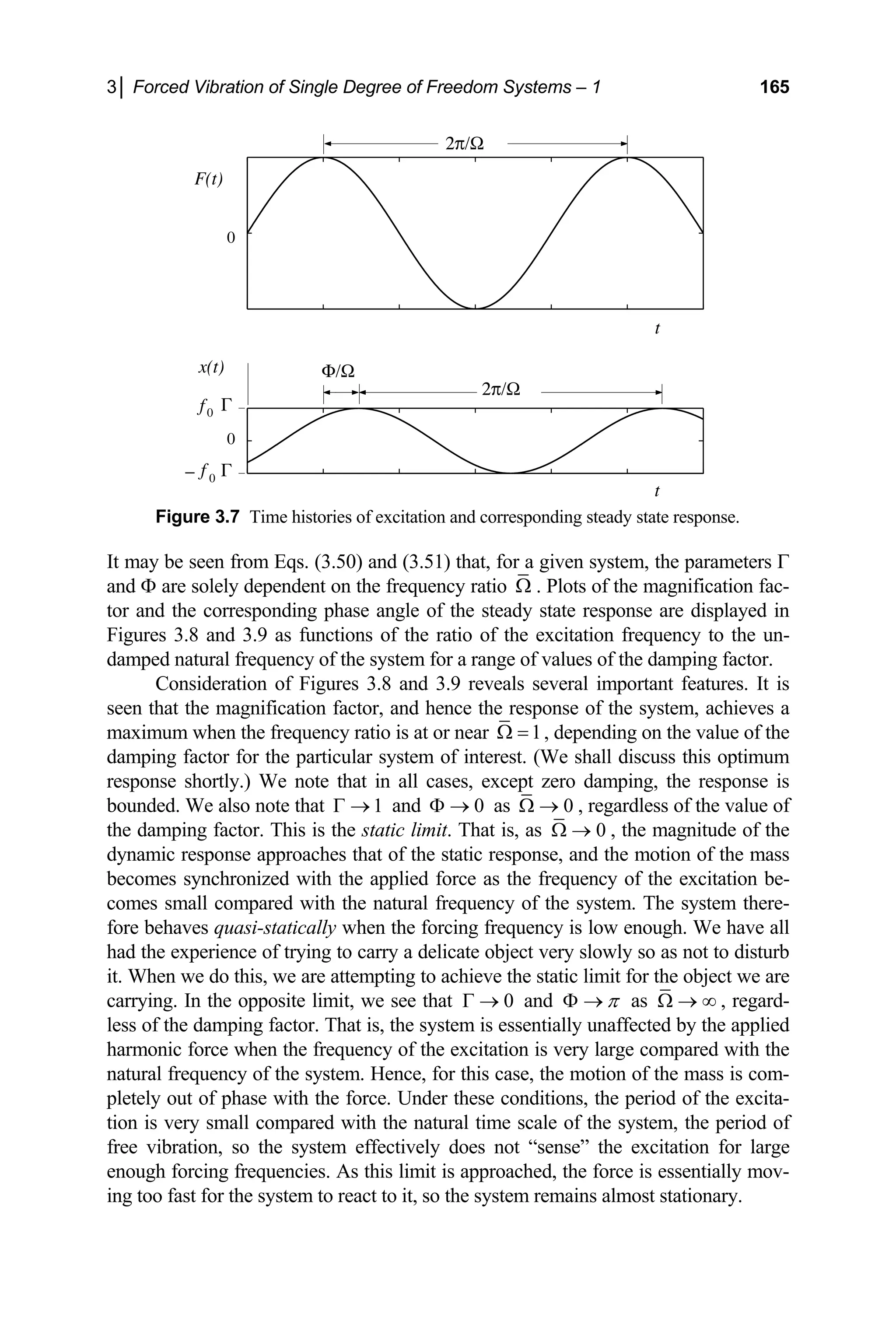
sponse are displayed as functions of time in Figure 3.7.
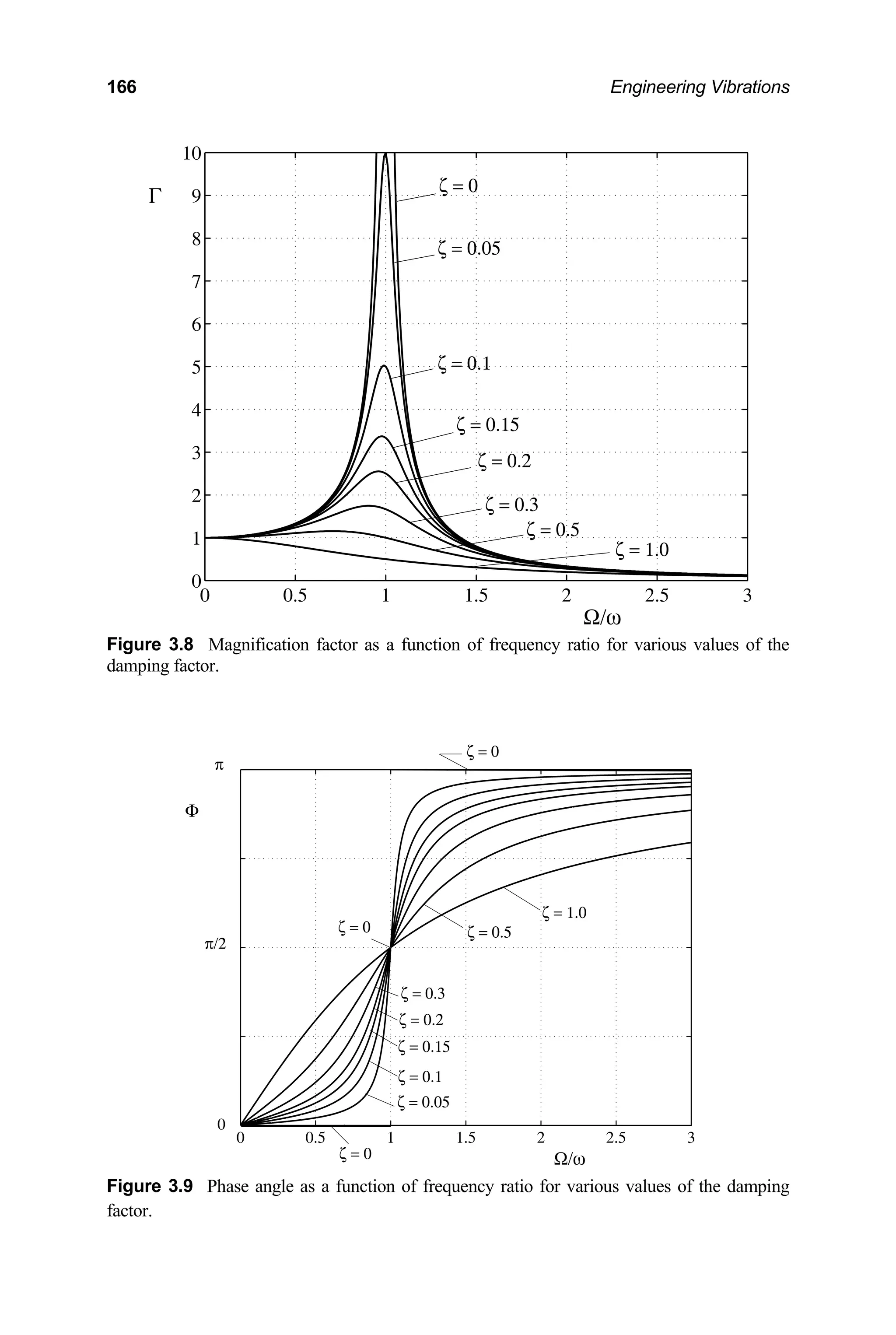
It may be seen from Eq. (3.49) that the parameter Γ corresponds to the ratio of
the amplitude of the dynamic response to that of the effective static response. For this
reason, Γ is referred to as the magnification factor as it is a measure of the magnifica-
tion of the response of the system to the harmonic force above the response of the
system to a static force having the same magnitude. Note that Eq. (3.24) is a special
case of Eq. (3.50). That is,
( ) ( )
0 ,0
Γ Ω = Γ Ω](https://image.slidesharecdn.com/engineeringvibrations-240713005818-b85f16c0/75/Engineering-Vibrations-Engineering-Vibrations-186-2048.jpg)
![168 Engineering Vibrations
3
0.5303
2 2(0.7071)(4)
c
m
ζ
ω
= = = (b)
2 2
1 0.7071 1 (0.5303) 0.5995 rad/sec
d
ω ω
= −ζ = − = (c)
Further, for each case,
0
0
5
2.5 m
2
F
f
k
= = = (d)
)
(a
For this case,
2
2.828
Ω
Ω = = =
0.7071
ω
(e)
For this excitation frequency the magnification factor is calculated as
( ) ( )
[ ]
2 2
2
2 2
2
1
1 2
1
0.1313
1 (2.828) 2(0.5303)(2.828)
ζ
Γ =
− Ω + Ω
= =
⎡ ⎤
− +
⎣ ⎦
(f)
We now calculate the corresponding amplitude of the steady state response,
(g)
et us compare the amplitude of the steady state response just calculated with
mplitude calculated in Example 3.2 for the same system without damping
e same excitation. For the undamped system the amplitude of the
culated to be X = 35.7 cm. We see that the damp-
ing has reduced the amplitude of the response by
equency.
or the case where the forcing frequency has the same value as the undamped
natural frequency,
0 (2.5)(0.1313) 0.3283 m 32.83 cm
X f
= Γ = = =
L
the a
subjected to th
steady state response was cal
about 3 cm at this excitation
fr
b)
(
F
1
Ω =
and hence,](https://image.slidesharecdn.com/engineeringvibrations-240713005818-b85f16c0/75/Engineering-Vibrations-Engineering-Vibrations-190-2048.jpg)
![3│ Forced Vibration of Single Degree of Freedom Systems – 1 169
1 1
0.9429
2 2(0.5303)
ζ
Γ → = = (h)
Thus, the amplitude of the steady state response when the excitation frequency
has the same value as the undamped natural frequency is
(2.5)(0.9429) 2.355 m
X = = (i)
)
For the case where the excitation frequency has the same value as the dam
atural frequency,
(c
ped
n
2
2
1
1 (0.5303) 0.8478
ω ζ
ω
−
Ω = = − = (j)
The magnification factor is then
[ ]
2 2
2
1.061
1 (0.8478) 2(0.5303)(0.8478)
⎡ ⎤
1
Γ = =
− +
agnitude of the steady state sponse for this excitation frequency is
⎣ ⎦
(k)
Thus, the m re
(2.5)(1.061) 2.653 m
X = = (l)
(d)
For the peak (resonance) response, the normalized excitation frequency is cal-
culated using Eq. (3.55). Hence,
2 2
1 2 1 2(0.5303) 0.6615
pk ζ
Ω = − = − = (m)
The magnification factor for the peak (resonance) response is next calculated to
be
[ ]
2 2
2
1
1.112 (n)
1 (0.6615) 2(0.5303)(0.6615)
Γ = =
⎡ ⎤
− +
⎣ ⎦
response at resonance is then
The amplitude of the steady state
(2.5)(1.112) 2.780 m
X = = (o)](https://image.slidesharecdn.com/engineeringvibrations-240713005818-b85f16c0/75/Engineering-Vibrations-Engineering-Vibrations-191-2048.jpg)
![3│ Forced Vibration of Single Degree of Freedom Systems – 1 171
We may determine the amplitude of the applied force from the amplitude
(b)
(The phase angle is unknown, but is merely a refe
rce that is 180˚ out of phase with the applied force will produce a response
of the observed response as follows. The observed response may be expressed
mathematically as
( ) sin( ) 0.6sin(2 ) m
obs obs obs
x t X t t
= Ω − Φ = − Φ
rence in this case. Note that a
fo
that is 180˚ out of phase with the observed motion and Eq. (a) will be satisfied.)
For the modified system,
2
0.5774 rad/sec
k
m
ω = = = (c)
6
and
3.7
0.5340
2 2(0.5774)(6)
c
m
ζ
ω
= = = (d)
Hence, for the observed steady state motion,
2
3.464
0.5774
Ω = = (e)
Now, from Eq. (3.49),
0
F
X f0
obs
k
= Γ = Γ (f)
Hence,
[ ]
0
2 2
2
(2)(0.6)
13.93 N
1 1 (3.464) 2(3.464)(0.5340)
obs
F = = =
Γ ⎡ ⎤
k X
− +
l force as the sine function
⎣ ⎦
(g)
If we reference the externa
0
( ) sin 13.93sin 2
F t F t t
= Ω = (h)
the actuator must apply the force
act
then
) N
( ) 13.93sin(2 ) 13.93sin(2
F t t t
π
= − = − (i)
to counter the effects of the excitation.](https://image.slidesharecdn.com/engineeringvibrations-240713005818-b85f16c0/75/Engineering-Vibrations-Engineering-Vibrations-193-2048.jpg)

![3│ Forced Vibration of Single Degree of Freedom Systems – 1 183
through resonance. The desired frequency range may also be achieved if the system
can be restrained during start-up, or a large amount of damping can be temporarily
imposed until the excitation frequency is sufficiently beyond the resonance fre-
quency. To close, it is seen that if the system is operated in the desired frequency
range and possesses low damping, then the vibrations of the system become isolated
from the surroundings. This is a very desirable result in many situations.
Example 3.10
Consider the system of Example 3.6. (a) Determine the magnitude of the force
transmitted to the support if the system is excited by the external force F(t) =
5sin2t N, where t is measured in seconds. Also determine the lag time of the re-
action force with respect to the applied force. (b) Determine the magnitude of
the transmitted force at resonance.
Solution
(a)
From Part (a) of Example 3.6, ζ = 0.5303, 2.828
Ω = and Γ= 0.1313. Substi-
tuting these values into Eq. (3.77) gives the transmissibility as
2
0.1313 1 [2(0.5303)(2.828)] 0.4151
= ϒ = + =
R
T
Thus, 42% of the applied force is transmitted to the support. The magnitude of
the force transmitted to the support is then, from Eq. (3.81),
(a)
0 (5)(0.4151) 2.076 N
tr
F F
= = =
R
T (b)
The corresponding phase angle is calculated using Eq. (3.78). Hence,
[ ]
3
1
2
2
2(.5303)(2.828)
tan 85.24 1.48 rads
1 (2.828) 2(.5303)(2
−
⎧ ⎫
8
.828)
⎪
⎪
⎪
Ψ = = ° =
⎨ ⎬
− +
⎪
⎩ ⎭
It follows that
(c)
1.488 2 0.7440 secs
lag
t = Ψ Ω = = (d)
(b)
For this case we have from Part (d) of Example 3.6 that 0.6615
Ω = and
Γ= 1.112. Thus,
2
1.112 1 [2(.5303)(0.6615)] 1.358
= + =
R
T (e)](https://image.slidesharecdn.com/engineeringvibrations-240713005818-b85f16c0/75/Engineering-Vibrations-Engineering-Vibrations-205-2048.jpg)
![3│ Forced Vibration of Single Degree of Freedom Systems – 1 189
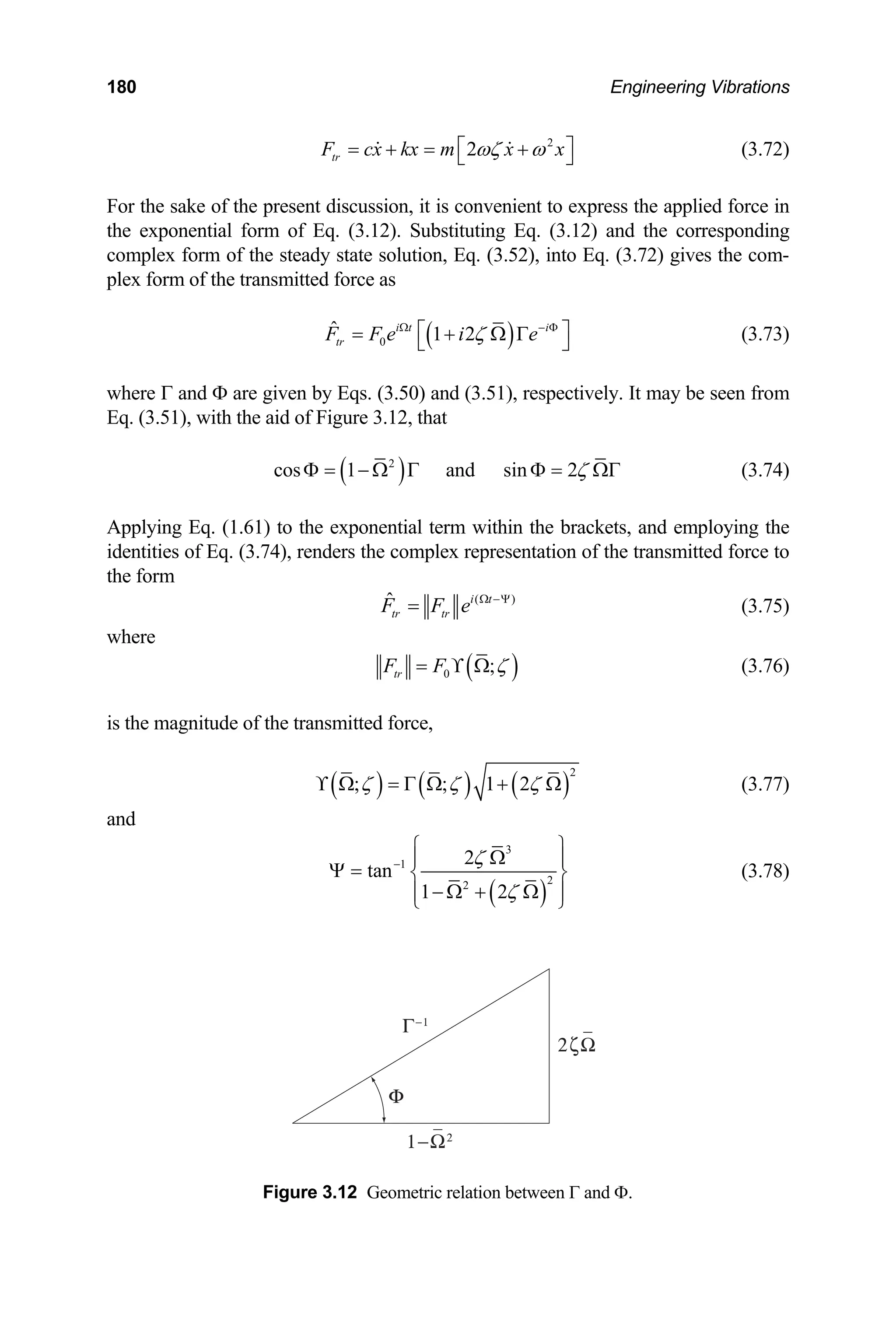
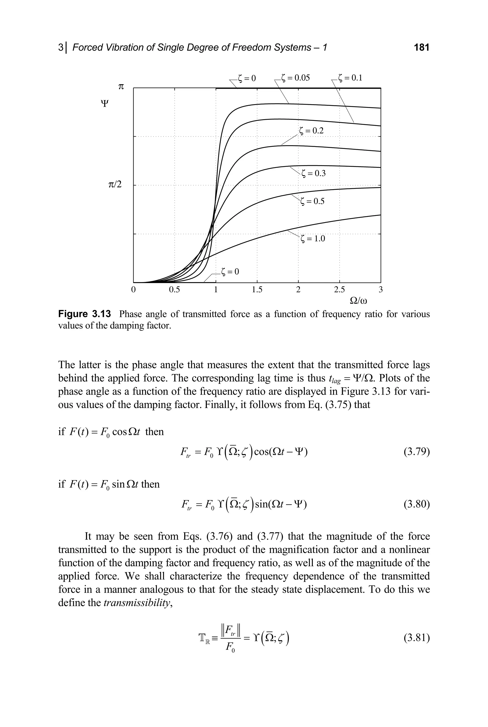
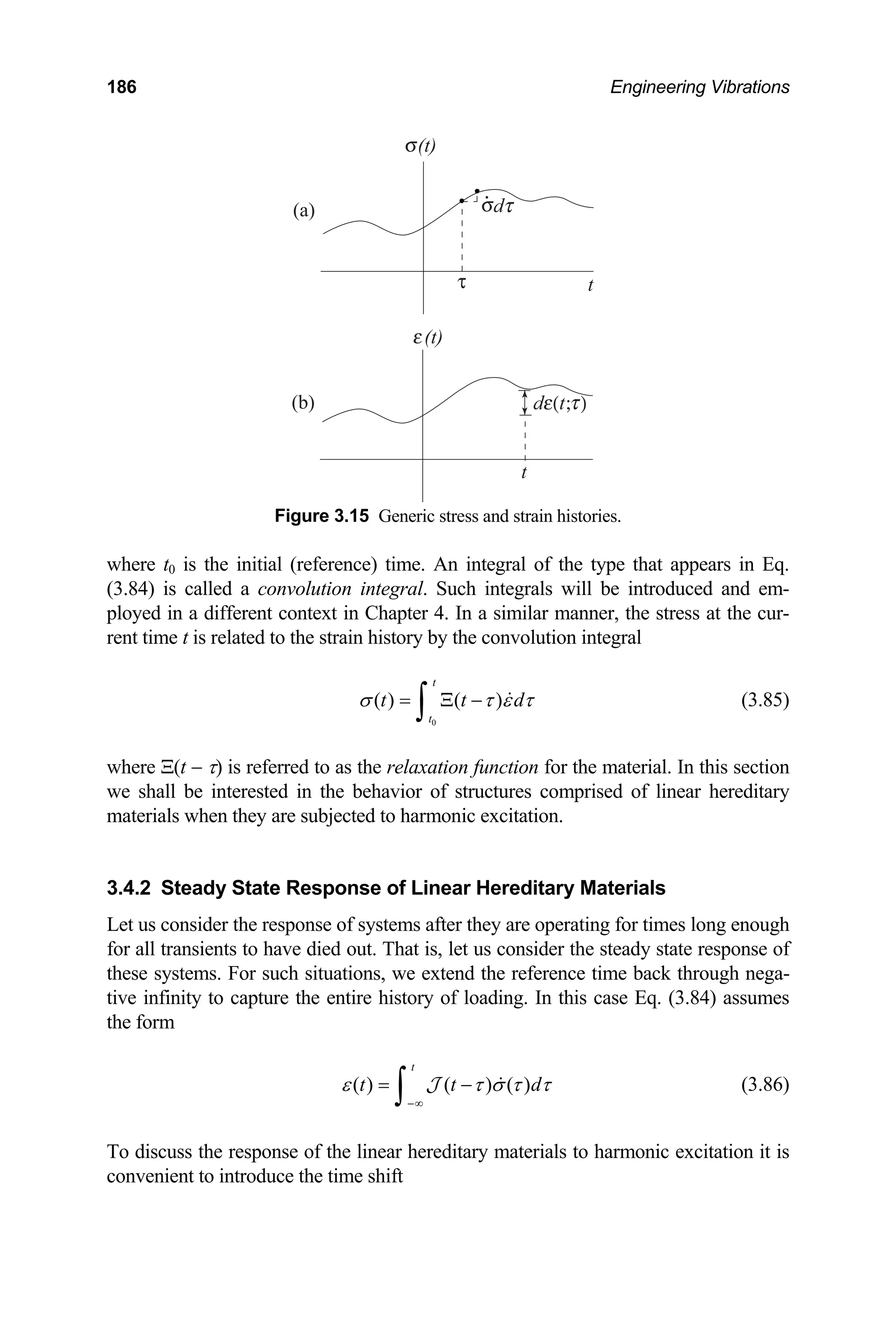
Figure 3.16 Kinetic diagram for structure.
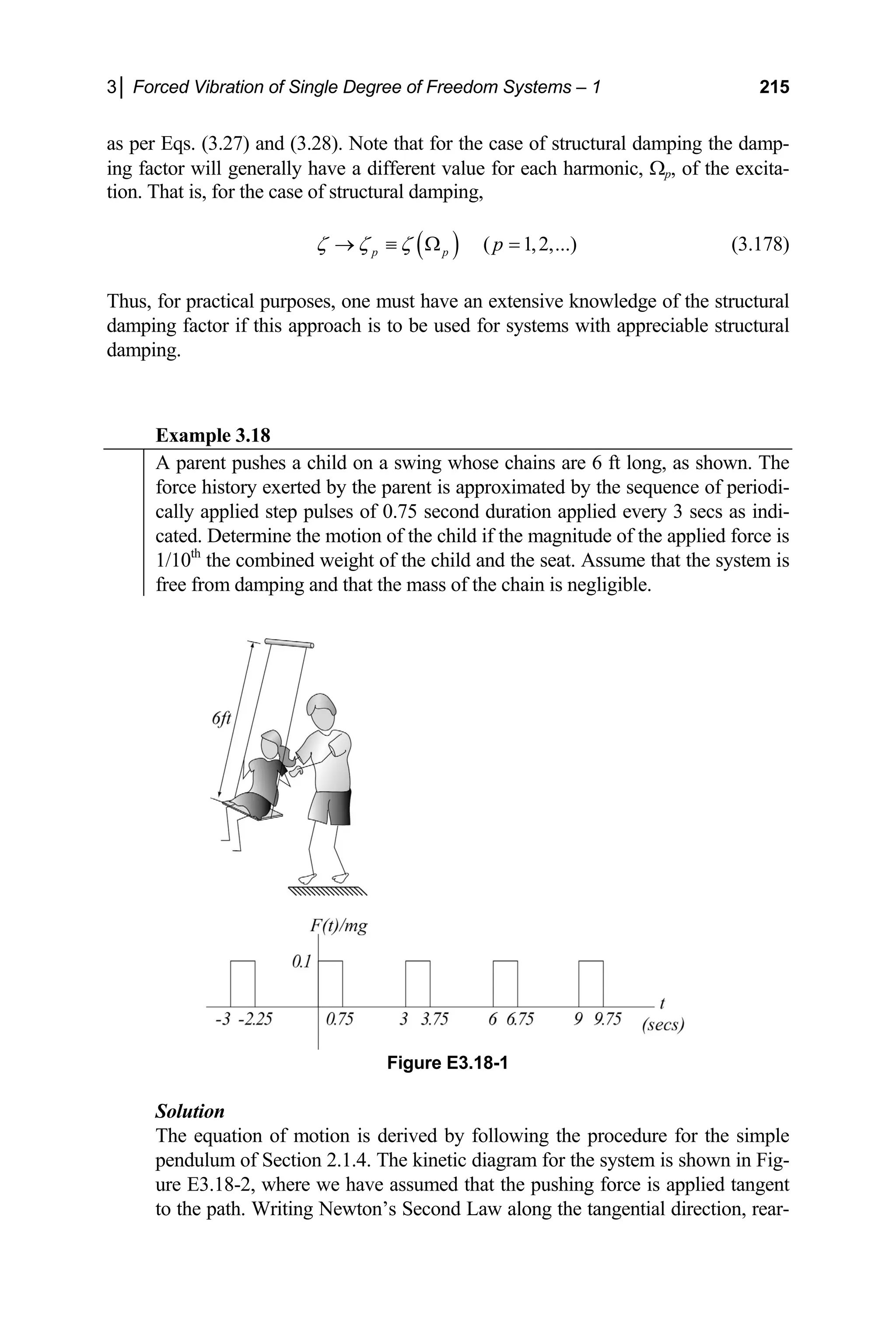
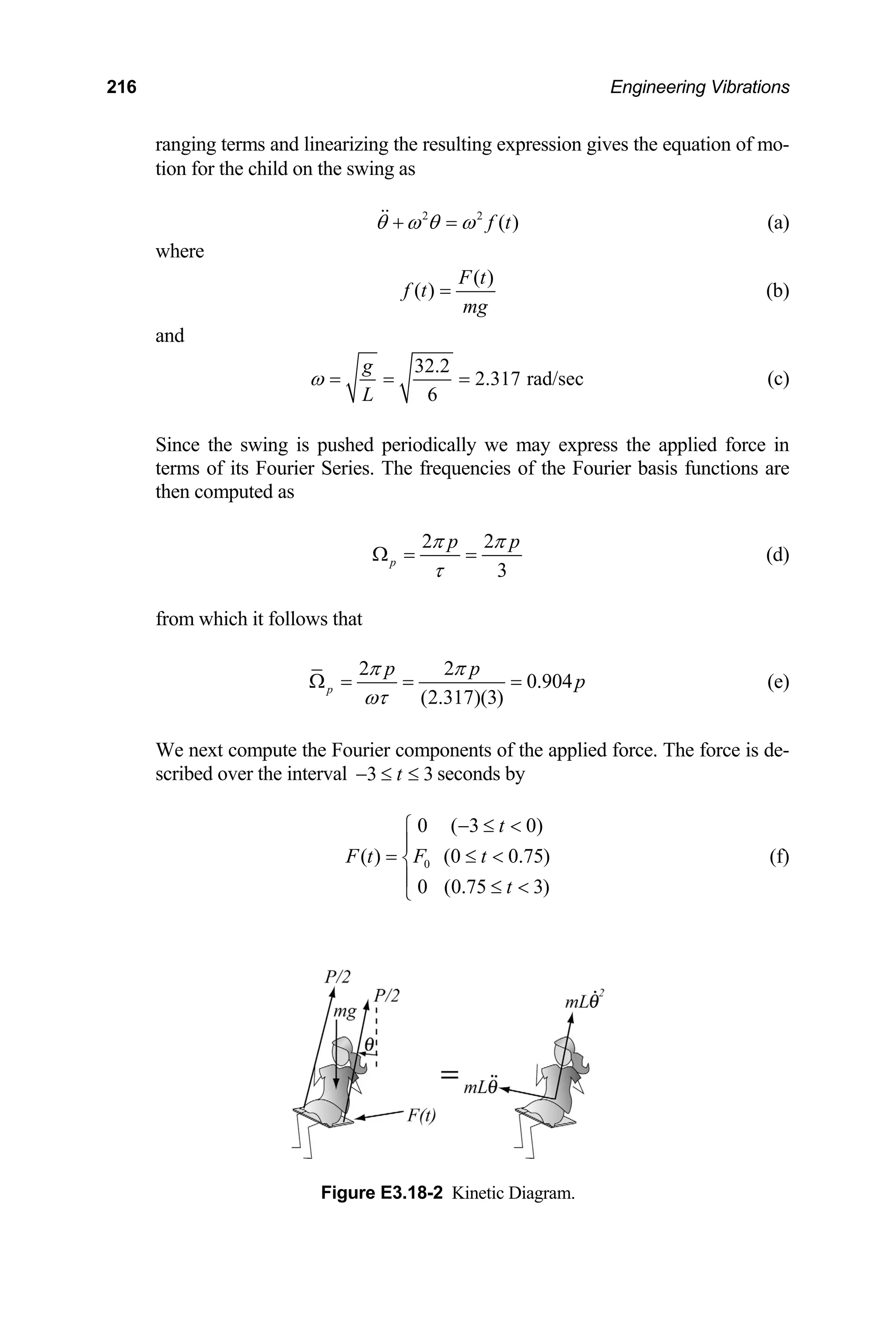
3.4.3 Steady State Response of Single Degree of Freedom Systems
When the mass of a structural member, such as a beam or rod, is small compared
with the other mass measures of a system, and we are primarily interested in the mo-
tion of a single point on that structure, we often approximate that system as an
equivalent single degree of freedom system. We next incorporate the effects of inter-
nal friction into such models.
If, in the equivalent single degree of freedom models of the elastic systems
discussed in Chapter 1 and employed to this point, we replace Young’s modulus, E,
and the shear modulus, G, by the complex elastic modulus, ˆ( ),
E Ω and complex shear
modulus, ˆ( ),
G Ω respectively defined by Eqs. (3.98) and (3.99), then the equivalent
iffness in each case will be replac
st ed by an equivalent com of the
plex stiffness, ˆ( ),
k Ω
form
[ ]
ˆ( ) ( ) 1 ( )
k k ik k iγ
Ω = + Ω = +
(3.100)
equivalent elastic stiffness as co
Ω
here k = constant is the mputed in Section 1.2 and
w
( ) ( )
k k
= Ω
(3.101)
is the structural loss factor. It follows from the corresponding dynamic free body
diagram (Figure 3.16) that the equation of motion for a ha
γ Ω
rmonically excited system
ith
w material damping takes the form of that for an undamped system with the spring
stiffness replaced by the complex stiffness defined by Eq. (3.100). If we introduce the
harmonic excitation in complex form, then the equation of motion for the correspond-
ing equivalent single degree of freedom system takes the form
0
ˆ
ˆ ˆ
( ) i t
mx k x F e Ω
+ Ω =
(3.102)
or equivalently
[ ]
2 2
0
ˆ ˆ
1 ( ) i t
x i x f e
ω γ ω Ω
+ + Ω =
(3.103)](https://image.slidesharecdn.com/engineeringvibrations-240713005818-b85f16c0/75/Engineering-Vibrations-Engineering-Vibrations-211-2048.jpg)
![198 Engineering Vibrations
5
3
48 1.11 10
42.3 rad/sec
(2000/32.2)
eff EI
m mL
ω
×
= = = = (b)
The excitation frequency is given as
k
4 cps 2 rads/cycle 8 rad/sec
π π
Ω = × = (c)
Thus,
8π
Ω = 0.594
42.3
= (d)
Now, to calculate the amplitude of the response using Eq. (3.128) we first com-
pute ϒ, giving
( )
( ) ( )
[ ]
[ ]
2 2
1 2 1 2(0.1)(0.594)
ζ
+ Ω +
ϒ = =
2 2 2 2
2 2
1.53
1 (0.594)
1 2ζ
=
⎡ ⎤
− +
− Ω + Ω ⎣ ⎦
(e)
he amplitude of the steady state response is
2(0.1)(0.594)
T then
0 2(1.53) 3.06
X h ′′
= ϒ = = (f)
The phase angle is next computed using Eq. (3.129) giving
( )
[ ]
3
1
2
2
2
2
tan
1 2
0.0633 rads
)
ζ
ζ
−
⎧ ⎫
Ω
⎪ ⎪
Ψ = ⎨ ⎬
− Ω + Ω
⎪ ⎪
⎩ ⎭
⎪
3
1
2
2(0.10)(0.594)
tan
1 (0.594) 2(0.1)(0.594
−
⎧ ⎫
⎪
= =
⎨ ⎬
⎪
− +
⎪
⎩ ⎭
(g)
0) gives the steady state response
Substituting Eqs. (c), (f) and (g) into Eq. (3.13
of the building,
( ) 3.06sin(8 0.0633)
ss
x t t (inches)
π
= −
The force transmitted to the support is compute
For 2
1
ζ we have
(h)
d from Eqs. (3.134) and (3.135).
5 2 3
0 (1.11 10 )(2/12) (0.594) (1.53) 9.99 10 lb
tr
F k h ⎡ ⎤
= = × = ×
⎣ ⎦
T (i)](https://image.slidesharecdn.com/engineeringvibrations-240713005818-b85f16c0/75/Engineering-Vibrations-Engineering-Vibrations-220-2048.jpg)
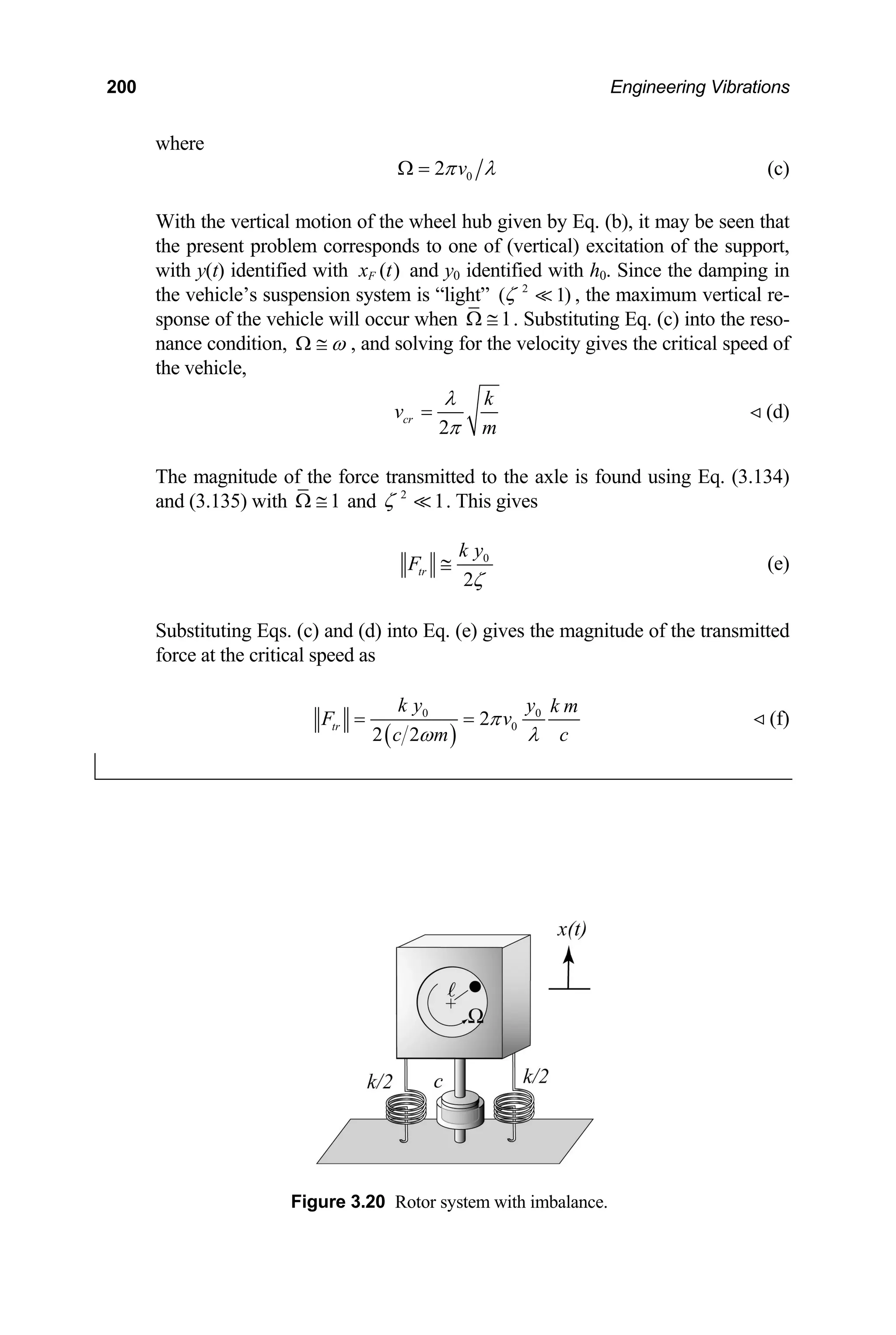
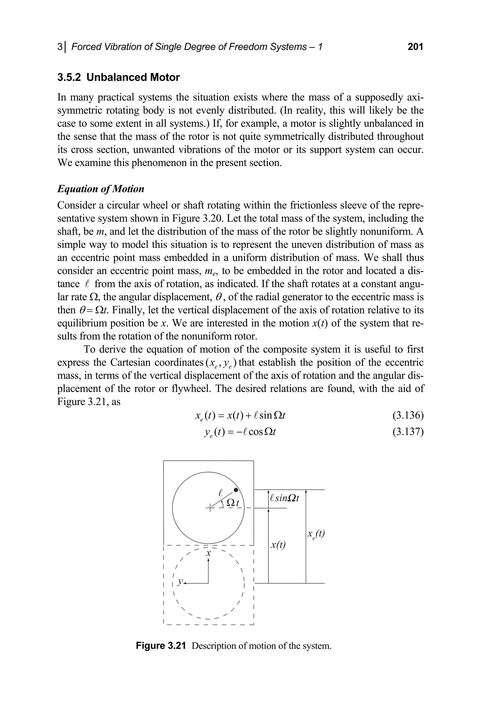
![202 Engineering Vibrations
We next isolate each of the bodies that comprise the idealized system. The corre-
In those diagrams the
mass of the rotor is labeled mw, and the resultant internal forces acting on the wheel,
lock are labeled
sponding dynamic free-body diagram is shown in Figure 3.22.
( )
,
w
F
G ( )
e
F
G
and ( )
,
b
F
G
respectively. A
the eccentric mass and the b
subscript x indicates the corresponding vertical component of that force. With the aid
of the kinetic diagrams, the vertical component of Newton’s Second Law may be
written for each body as
[ ]
( )
b
x e w
F kx cx m m m x
− − = − −
( ) 2
sin
e
x e e
F m x m x t
⎡ ⎤
= = − Ω Ω
⎣ ⎦ (3.138)
A
( )
w
x w
F m
=
x
We next sum Eqs. (3.138) and note that the internal forces sum to zero via Newton’s
Third Law. This results in the governing equation for the vertical motion of the entire
system
2
sin
e
mx cx kx m t
+ + = Ω Ω
A (3.139)
When rearranged, Eq. (3.139) takes the standard form
2 2
0
2 sin
x x x f t
ωζ ω ω
+ + = Ω
(3.140)
where
( ) 2
0 0
e
f f
m
m
= Ω = Ω (3.141)
A
Figure stem.
3.22 Kinetic diagram for each component of the sy](https://image.slidesharecdn.com/engineeringvibrations-240713005818-b85f16c0/75/Engineering-Vibrations-Engineering-Vibrations-224-2048.jpg)
![3│ Forced Vibration of Single Degree of Freedom Systems – 1 205
64
4 rad
4
k
m
ω = = = /sec (a)
and
6.4
0.2
2 2(4)(4)
c
m
ζ
ω
= = = (b)
Therefore,
6
1.5
4
ω
Ω
Ω = = = (c)
Substituting Eqs. (b) and (c) into Eq. (3.143) gives the ratio of the first inertial
moments as
[ ]
2
2
2 2
2
(1.5)
1.623
1 (1.5) 2(1.5)(0.2)
= Ω Γ = =
⎡ ⎤
− +
Rearranging Eq. (3.143) and substituting Eq. (d) gives the offset moment
⎣ ⎦
Q (d)
(4)(0.05)
0.1232 kg-m
1.623
e
mX
m = = =
A
Q
(e)
(b)
To determine the magnitude of the transmitted force, we simply substitute the
given displacement and effective stiffness, as well as the computed damping
factor and frequency ratio, into Eq. (3.147). Ca
magnitude of the force transmitted to t
rrying through the computation
he support as
gives the
[ ]
2
(64)(0.05) 1 2(0.2)(1.5) 3.732 N (f)
tr
F = + =
Example 3.16
Determine the amplitude of the response of the system of Example 3.15 when
the rotation rate is increased to 60 rad/sec.
Solution
For this case,
60
15
4
Ω = = (a)
and hence](https://image.slidesharecdn.com/engineeringvibrations-240713005818-b85f16c0/75/Engineering-Vibrations-Engineering-Vibrations-227-2048.jpg)
![206 Engineering Vibrations
2
225 1
Ω = (b)
herefore and
1
≈
Q
T
0.1232
0.03080 m 3.08 cm
4
e
m
X
m
≈ = = =
A
(c)
Let us next calculate the amplitude using the “exact” solution. Hence,
[ ]
2
2
2
(15)
1.004
1 (15) 2(0.2)(1
= =
⎡ ⎤
− +
⎣ ⎦
Q (d)
2
5)
The amplitude of the steady state response is then
0.1232
(1.004) 0.03092 m 3.09 cm
4
e
m
X
m
= = = =
A
Q (e)
Comparing the two answers we see that the error in using the large frequency
pproximation is
a
3.09 3.08
% error 100% 0.324%
3.09
−
= × = (f)
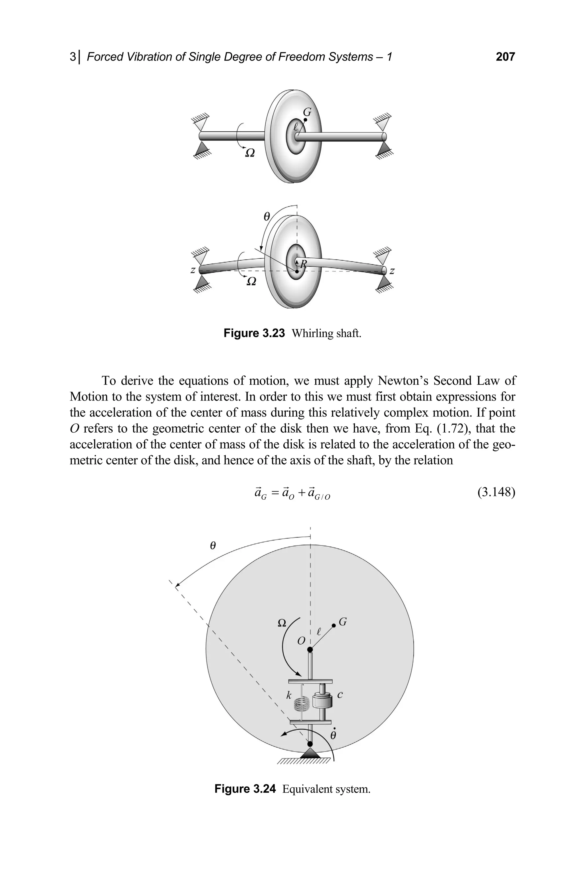
3.5.3
Cons
tic sh k be offset a dis-
tance m the axis of the shaft as shown, and let the shaft-disk system be spinning
bout its axis at the angular rate Ω. Further let the mass of the shaft be very sm
mpared with the mass of the disk and thus be considered negligible. The system
may then be modeled as an equivalent single degree of freedom system as shown in
Figure 3.24. In this regard, let k represent the equivalent elastic stiffness of the shaft
bending (Section 1.2.2), and let c represent some effective viscous damping of the
system y be provided, for example, by oil in the bearings, by structural
damp
proble
Synchronous Whirling of Rotating Shafts
ider a circular disk of mass m that is coaxially attached at center span of an elas-
aft as shown in Figure 3.23. Let the center of mass of the dis
ℓ fro
a all
co
in
. The latter ma
ing (Section 3.4) or by aerodynamic damping (Section 1.2.6). To examine this
m, we first derive the equations of motion for the disk during whirl.](https://image.slidesharecdn.com/engineeringvibrations-240713005818-b85f16c0/75/Engineering-Vibrations-Engineering-Vibrations-228-2048.jpg)
![210 Engineering Vibrations
ized amplitude of whirling as a function of the normalized spin rate and the damping
factor. Hence,
( )
2
;
R
R ζ
≡ = Ω Γ Ω
A
(3.157)
It may be seen that the normalized amplitude given by Eq. (3.157) is of the identical
functional form as Eq. (3.121). The associated plots displayed in Figure 3.19 there-
fore describe the normalized amplitude for the problem of synchronized whirl, as
well. Recall, however, that for structural damping the damping factor is dependent on
the excitation frequency.
xam .
E ple 3 17
A 50 lb rotor is mounted at center span of a 6 ft shaft having a bending stiffness
of lb-in2
. The shaft is supported by rigid bearings at each end. When
6
20 10
×
operating at 2000 rpm the shaft is strobed and the rotor is observed to displace
off-axis by ½ inch. If the damping factor for the system is 0.1 at this frequency,
determine the offset of the rotor.
Solution
The effective stiffness for transverse motion of the shaft is determined using
Eq. (1.17) to give
6
3 3 3
12 (20 10 )
2 192 192 10,290 lb/in
( / 2) (6 12)
EI EI
k
L L
×
= × = = =
×
(a)
(See Problem 1.14.) The natural frequency of the system is then computed to be
10,290
282 rad/sec
50/(32.2 12)
ω = =
×
(b)
The rotation rate of the rod is given as
2000rev/min 2 rad/rev 1min/60sec 209 rad/sec
π
Ω = × × = (c)
Hence,
209
0.741
282
Ω = = (d)
Now,
[ ]
2
2
2 2
2
(0.741)
1.16
Ω Γ = = (e)
1 (0.741) 2(0.10)(0.741)
⎡ ⎤
− +
⎣ ⎦](https://image.slidesharecdn.com/engineeringvibrations-240713005818-b85f16c0/75/Engineering-Vibrations-Engineering-Vibrations-232-2048.jpg)
![3│ Forced Vibration of Single Degree of Freedom Systems – 1 213
( )
f t i
Let us express the excitation function n terms of its Fourier series. Hence,
0
1 1
( ) cos sin
( ) ( )
c s
p p p p
p p
f t f f t f t
= =
= + Ω + Ω
∑ ∑ (3.163)
here
∞ ∞
w
2
( 1,2,...)
p
p
p
π
τ
Ω = = (3.164)
nd the associated Fourier components are given by
a
/ 2
0
/ 2
1
( )
f f t dt
τ
τ
τ −
=
∫ (3.165)
which is seen to be the average value of the excitation ( )
f t over a period, and
/ 2
( ) 2
( )cos ( 1,2,...)
c
p p
f f t t dt p
τ
τ
= Ω =
∫ (3.166)
/ 2
τ
−
d
an
/ 2
( )
/ 2
2
( )sin ( 1,2,...)
s
p p
f f t t dt p
τ
τ
τ −
= Ω =
∫ (3.167)
which are the Fourier coefficients (components) of the cosine and sine basis func-
tions, respectively. These coefficients are thus the components of the given forcing
function with respect to the harmonic basis functions. [The equations for the Fourier
omponents arise fro
c m multiplying Eq. (3.163) by cos pt
Ω or sin pt
Ω , then integrat-
period τ and incorporating Eqs. (3.160)–(3.162).] At this point we are
minded of certain characteristics regarding convergence of a Fourier series repre-
ntation, particularly for functions that possess discontinuities. Notably, that the
average value of the func-
on at points of discontinuity, and that the series does not converge uniformly.
if the series for such a function is truncated, the partial sums
henomenon whereby overshoots (bounded oscillatory spikes) relativ
occur in the vicinity of the discontinuity. With the Fourier series of an arbitrary peri-
odic excitation established, we now proceed to obtain the general form of the corre-
ing steady state response.
Steady State Response
We next substitute the Fourier series for the excitation into the equation of motion for
the system. The equation of motion then takes the form
ing over the
re
se
Fourier series of a discontinuous function converges to the
ti
Rather, exhibit Gibbs
P e to the mean
spond
3.6.2](https://image.slidesharecdn.com/engineeringvibrations-240713005818-b85f16c0/75/Engineering-Vibrations-Engineering-Vibrations-235-2048.jpg)
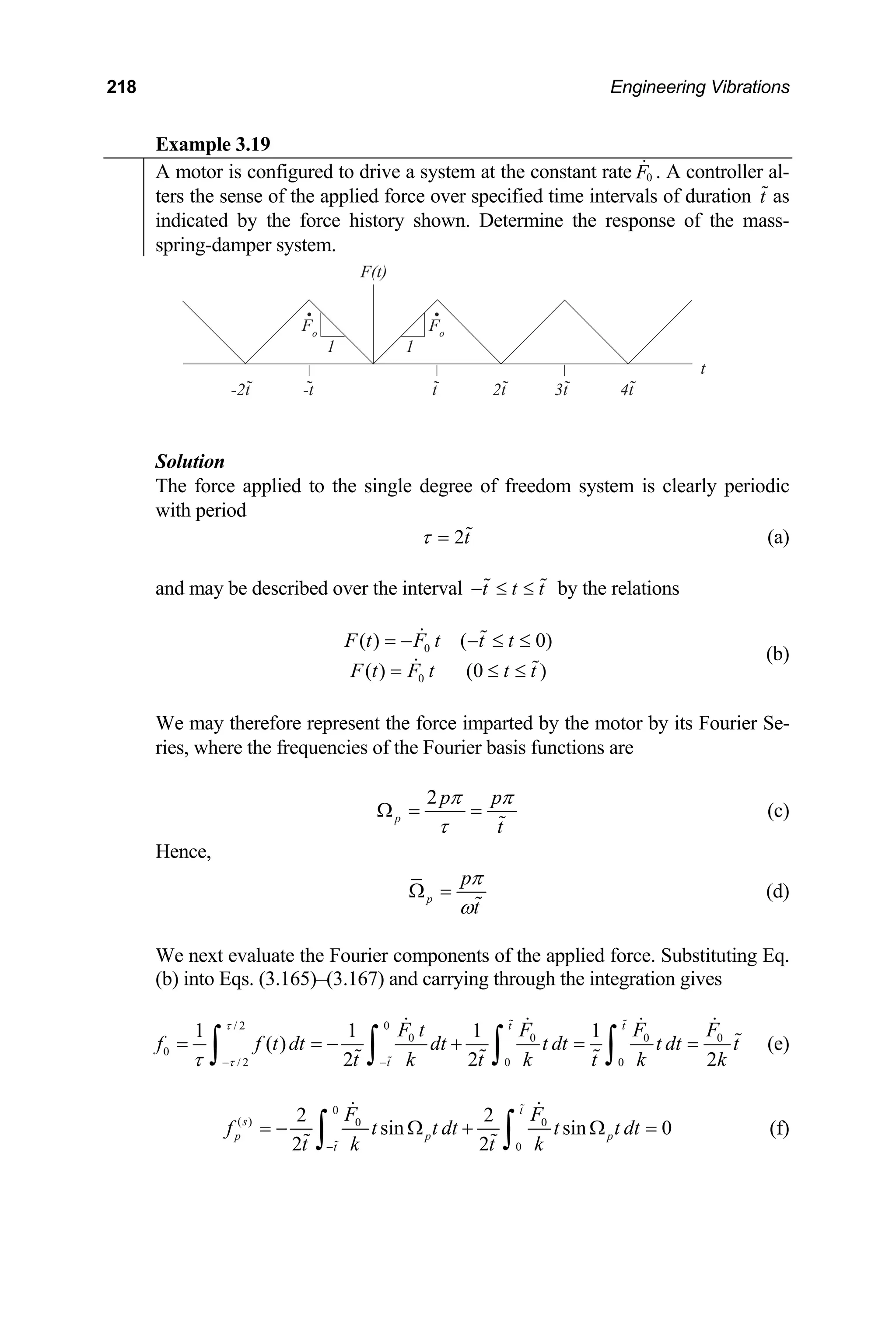
![3│ Forced Vibration of Single Degree of Freedom Systems – 1 217
Substituting Eq. (f) into Eqs. (3.165)–(3.167) and carrying through the integra-
tion gives
/ 2 0 0.75 1.5
0 1
0
F
dt dt
+
∫
0
/ 2 1.5 0 0.75
0
1 1 1
( ) 0
3 3 3
(0.1)
0.025
4 4
f f t dt dt
mg
F mg
τ
τ
τ − −
= = +
= = =
∫ ∫ ∫ (g)
f0 is the average value of f over a period),
(note that
/ 2
( )
/ 2
0 0.75 1.5
0
1.5
2 2 2
0 cos cos 0 cos
3
p p p
F
t dt t dt t dt
τ
τ −
−
= ⋅ Ω + Ω + ⋅ Ω
∫ ∫ ∫ (h)
0 0.75
2
( )cos
3 3
sin( / 2)
0.1
c
p p
f f t t dt
mg
p
p
τ
π
π
= Ω
=
∫
and
/ 2
( ) 2
s
τ
/ 2
0 0.75
0
1.5 0 1.5
( )sin
2 2
0 sin sin
3 3 3
p p
p p p
f f t t dt
F
t dt t d
mg
τ
τ
π
−
− −
= Ω
= ⋅ Ω + Ω +
∫
∫ ∫ ∫
Substituting Eqs. (d)–(i) into Eqs. (3.169), (3.170), (3.176) and (3.177) gives
onse of the child and swing,
0
2
0 sin
t t dt
⋅ Ω (i)
[1 cos( / 2)]
0.1
p
p
π
−
=
the steady state resp
[ ]
{ }
2
1
( ) 0.025
0.1 1
+ sin( / 2)cos(2 /3) 1 cos( / 2) sin(2 /3)
(1 0.816 )
ss
p
t
p p t p p t
p p
θ
π π π π
π
∞
=
=
+ −
−
∑
radi (j)
ans](https://image.slidesharecdn.com/engineeringvibrations-240713005818-b85f16c0/75/Engineering-Vibrations-Engineering-Vibrations-239-2048.jpg)
![3│ Forced Vibration of Single Degree of Freedom Systems – 1 219
0
( ) 2
c F
[ ]
0 0
0 0
1
0 0
2 2 2 2
cos cos cos
2 2
2 2
1 cos 1 ( 1)
p p p p
t
p
0
2 2
t t
F F
f t t dt t t dt t t dt
t k t k t k
F t F t
p
p k p k
π
π π
−
+
= − Ω + Ω = Ω
⎡ ⎤
= − − = − + −
⎣ ⎦
∫ ∫ ∫
With the Fourier components of the applied force calculated, we now deter-
mine the steady state response of the system by substituting Eqs. (d)–(g) into
Eqs. (3.169)–(3.175). In doing so we obtain the steady state response of the
system as
(g)
1
0
2 2
1
4 1 ( 1)
( ) 1 cos( / )
2
p
ss p
p
F t
x t p
k p
π
π
∞ +
=
t t
⎡ ⎤
+ −
⎢ ⎥
= − Γ
⎢ ⎥
⎣ ⎦
∑
(h)
where
( ) ( )
2
2
1
p
p t
π ω
Γ =
⎡ ⎤
1
2
2 p t
ζ π ω
⎡ ⎤
+
− ⎣ ⎦
⎢ ⎥
⎣ ⎦
(i)
3.7 CONCLUDING REMARKS
In thi freedom systems
that ar citation, that is excitation that repeats itself at regular
time. We began by studying sy
cted to external forces that vary harmonically in ti
onding to motion of the support, unbalanced motors and synchro-
ating shafts. In each case the steady state response was seen to be
rongly influenced by the ratio of the excitatio
undamped motion, and the viscous damping factor. A notable feature is the phe-
nomenon of resonance whereby the mass of the system undergoes large amplitude
motio
tems ncy. It
was seen that at resonance the work of the external force is used in the optimal man-
ndamped systems the amplitude of the steady state response was seen to
row linearly with time. The related phenomenon of beating was seen to occu
stems with vanishing damping, when the excitation frequency was very close to but
ot equal to the natural frequency. In this case the system is seen to oscillate at the
verage between the excitation and natural frequency, with the amplit
monically with very large period. For viscously damped systems the peak re-
sponse was seen to occur at values of the excitation frequency away from the un-
damped natural frequency, and at lower frequencies for a force excited system, the
damping slowing the system down. We remark that in some literature the term reso-
s chapter we have considered the motion of single degree of
e subjected to periodic ex
intervals over long periods of stems which were sub-
je me. We also considered classes of
applications corresp
nous whirling of rot
st n frequency to the natural frequency
n when the excitation frequency achieves a critical value. For undamped sys-
this occurs when the forcing frequency is equal to the excitation freque
ner. For u
g r, for
sy
n
a ude oscillating
har](https://image.slidesharecdn.com/engineeringvibrations-240713005818-b85f16c0/75/Engineering-Vibrations-Engineering-Vibrations-241-2048.jpg)

![4│ Forced Vibration of Single Degree of Freedom Systems – 2 235
(4.18)
0 0
lim ( ) 0
t
t
F t dt
∆
∆ →
→
∫
With the mathematical description of impulsive and nonimpulsive forces established,
we next determine the general response of a standard single degree of freedom sys-
tem to an arbitrary impulsive force.
4.2.2 Response to an Applied Impulse
Consider a mass-spring-damper system that is initially at rest when it is subjected to
an impulsive force F(t), as shown in Figure 4.4. Let us next apply the principle of
linear impulse-momentum, Eq. (1.96), to the initially quiescent system over the time
interval when the impulsive force defined by Eq. (4.17) is applied. Hence,
[ ]
0 0
0 0
( ) (0 ) (0 )
t dt kx cx dt m x x
δ
+ +
− −
+ −
⎡ ⎤
− + = −
⎣ ⎦
∫ ∫
I (4.19)
where m, k and c correspond to the mass, spring constant and damping coefficient of
the system, respectively. Since the spring force and damping force are nonimpulsive
forces, the second integral on the left-hand side of Eq. (4.19) vanishes. Since the sys-
tem is initially at rest, the corresponding initial velocity is zero as well. The impulse-
momentum balance, Eq. (4.19), then reduces to the relation
(0 )
mx +
=
I (4.20)
If we consider times after the impulsive force has acted (t 0) then, using Eq. (4.20)
to define the initial velocity, the problem of interest becomes equivalent to the prob-
lem of free vibrations with the initial conditions
Figure 4.4 Mass-spring-damper system subjected to an impulsive force.](https://image.slidesharecdn.com/engineeringvibrations-240713005818-b85f16c0/75/Engineering-Vibrations-Engineering-Vibrations-257-2048.jpg)
![4│ Forced Vibration of Single Degree of Freedom Systems – 2 237
Solution
The damping factor, natural frequency and natural period are easily computed
to be (see Example 2.11)
2
400 4 10 rad/sec, 16 [2(10)(4)] 0.2,
10 1 (0.2) 9.798 rad/sec, 2 9.798 0.6413 secs
d d
T
ω ζ
ω π
= = = =
= − = = =
(a)
(a)
The unit step response for the system is computed from Eq. (4.23) giving
(0.2)(10)
2
1
( ) sin(9.798 ) ( )
(4)(9.798)
0.02552 sin(9.798 ) ( ) (m/N-sec)
t
t
t e t
e t t
−
−
=
=
G H
H
t
⎦
(b)
Substitution of the given impulse and Eq. (b) into Eq. (4.22) gives the response
of the system as
(c)
2
2
( ) (2) 0.02552 sin(9.798 ) ( )
0.05104 sin(9.798 ) ( ) (meters)
t
t
x t e t t
e t t
−
−
⎡ ⎤
= ⎣
=
H
H
Hence,
2
( ) 0 ( 0)
( ) 0.05104 sin(9.798 ) ( 0)
t
x t t
x t e t t
−
=
=
(d)
(b)
The response of the system to the two impulses is the sum of the response to
each impulse applied individually. Hence,
(e)
{ }
2
2( 10)
( ) 0.05104 sin(9.798 ) ( )
sin 9.798( 10) ( 10) (m)
t
t
x t e t t
e t t
−
− −
⎡
= ⎣
⎤
+ − − ⎦
H
H
Thus,
{ }
2
2 2( 10)
( ) 0 (m) ( 0)
( ) 0.05104 sin(9.798 ) (m) (0 10 secs)
( ) 0.05104 sin(9.798 ) sin 9.798( 10) (m) ( 10 secs)
t
t t
x t t
x t e t t
x t e t e t t
−
− − −
=
=
⎡ ⎤
= + −
⎣ ⎦
(f)](https://image.slidesharecdn.com/engineeringvibrations-240713005818-b85f16c0/75/Engineering-Vibrations-Engineering-Vibrations-259-2048.jpg)
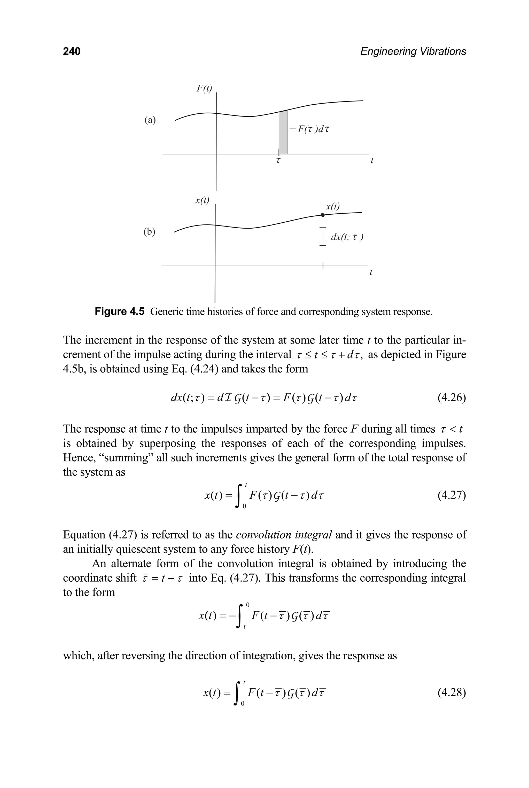
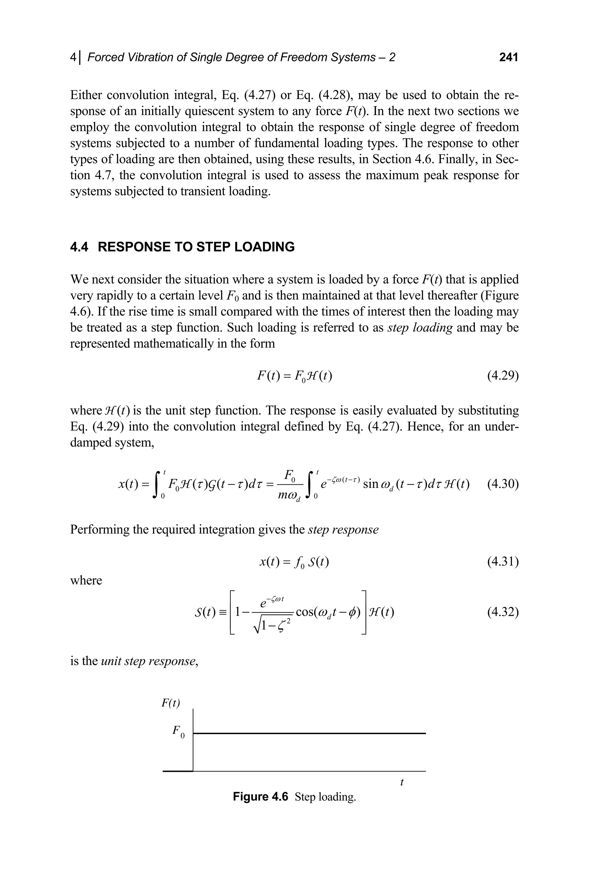
![242 Engineering Vibrations
0 0
f F k
= (4.33)
for a mass-spring-damper system,
2
1
d
ω ω ζ
= − (4.34)
and
1
2
tan
1
ζ
φ
ζ
−
⎧ ⎫
⎪ ⎪
= ⎨ ⎬
−
⎪ ⎪
⎩ ⎭
(4.35)
Example 4.3
The beam and mass system of Example 3.4 is ini-
tially at rest when an actuator suddenly applies a
constant downward force whose magnitude is half
the weight of the system. Determine the motion of
the beam and block. Plot the time history of the re-
sponse.
Figure E4.3-1
Solution
From Example 3.4, m = 10 kg and ω = 6π rad/sec. Hence,
(a)
2 2
(6 ) (10) 360 N/m
k π π
= =
We shall take the time at which the force is first applied to the structure as t = 0.
Now, the magnitude of the applied force is simply half the weight of the block.
Further, since the force is applied suddenly, its time dependence may be taken
as a step function. Thus,
1 1
0 2 2
( ) ( ) ( ) (10)(9.81) ( ) 49.1 ( ) N
F t F t mg t t t
= = − = − = −
H H H H (b)
It follows that
0
0 2
49.1
0.0138 m
360
F
f
k π
−
= = = − (c)
Substitution of the Eq. (c) and the known natural frequency into Eq. (4.31),
with ζ = 0, gives the motion of the system as
( ) 0.0138[1 cos6 ] ( ) m
1.38[1 cos6 ] ( ) cm
x t t t
t t
π
π
= − −
= − −
H
H
(d)](https://image.slidesharecdn.com/engineeringvibrations-240713005818-b85f16c0/75/Engineering-Vibrations-Engineering-Vibrations-264-2048.jpg)
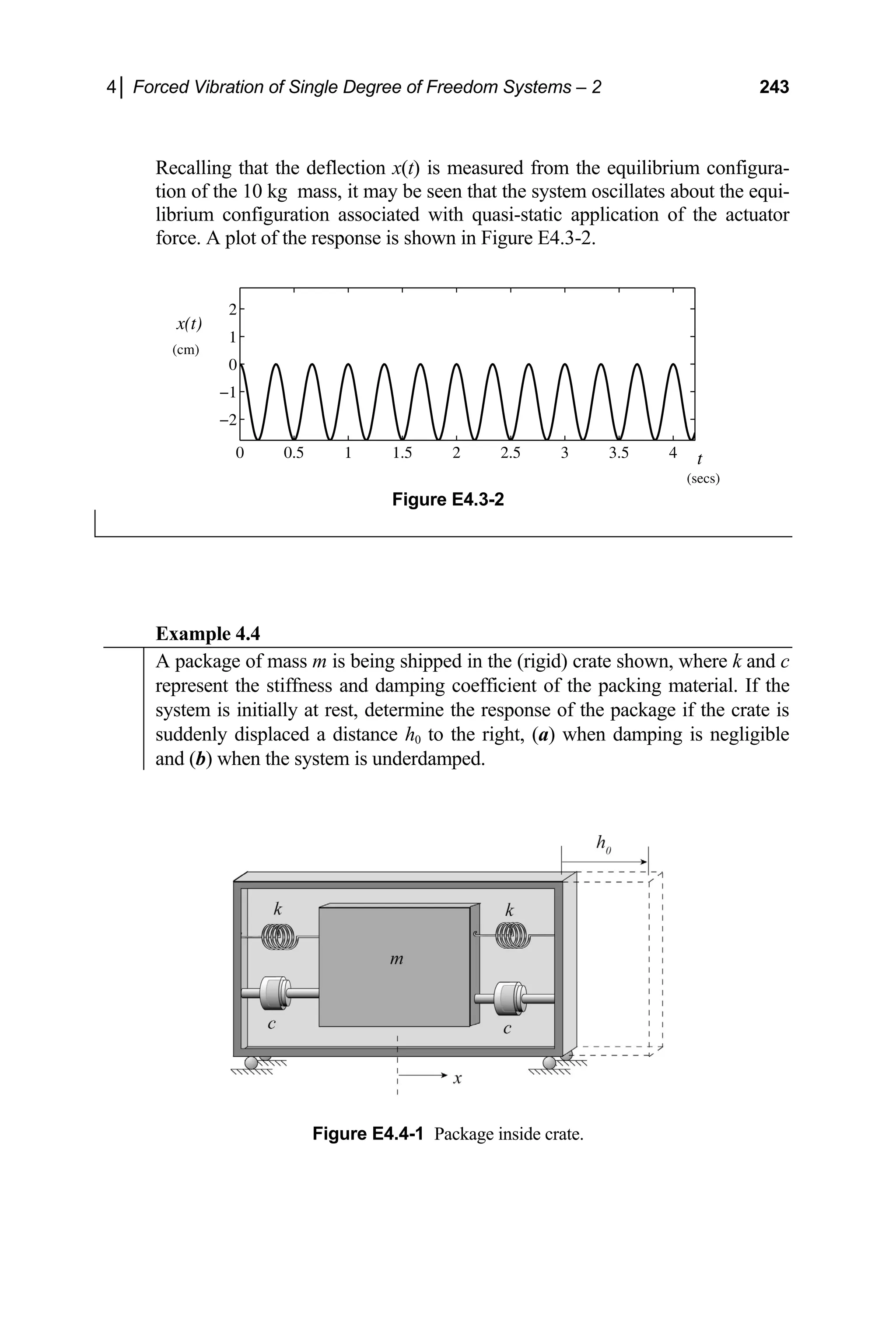
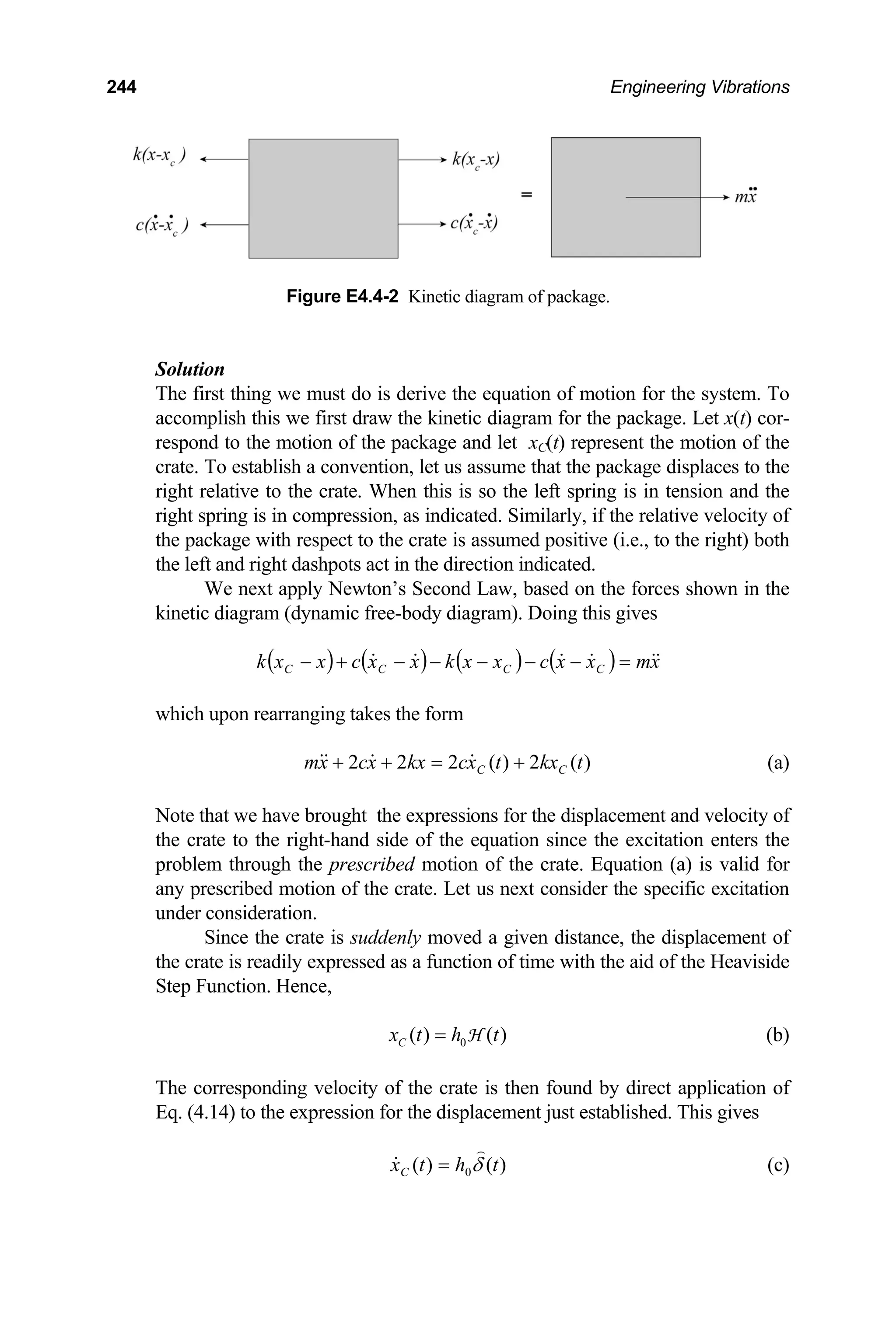
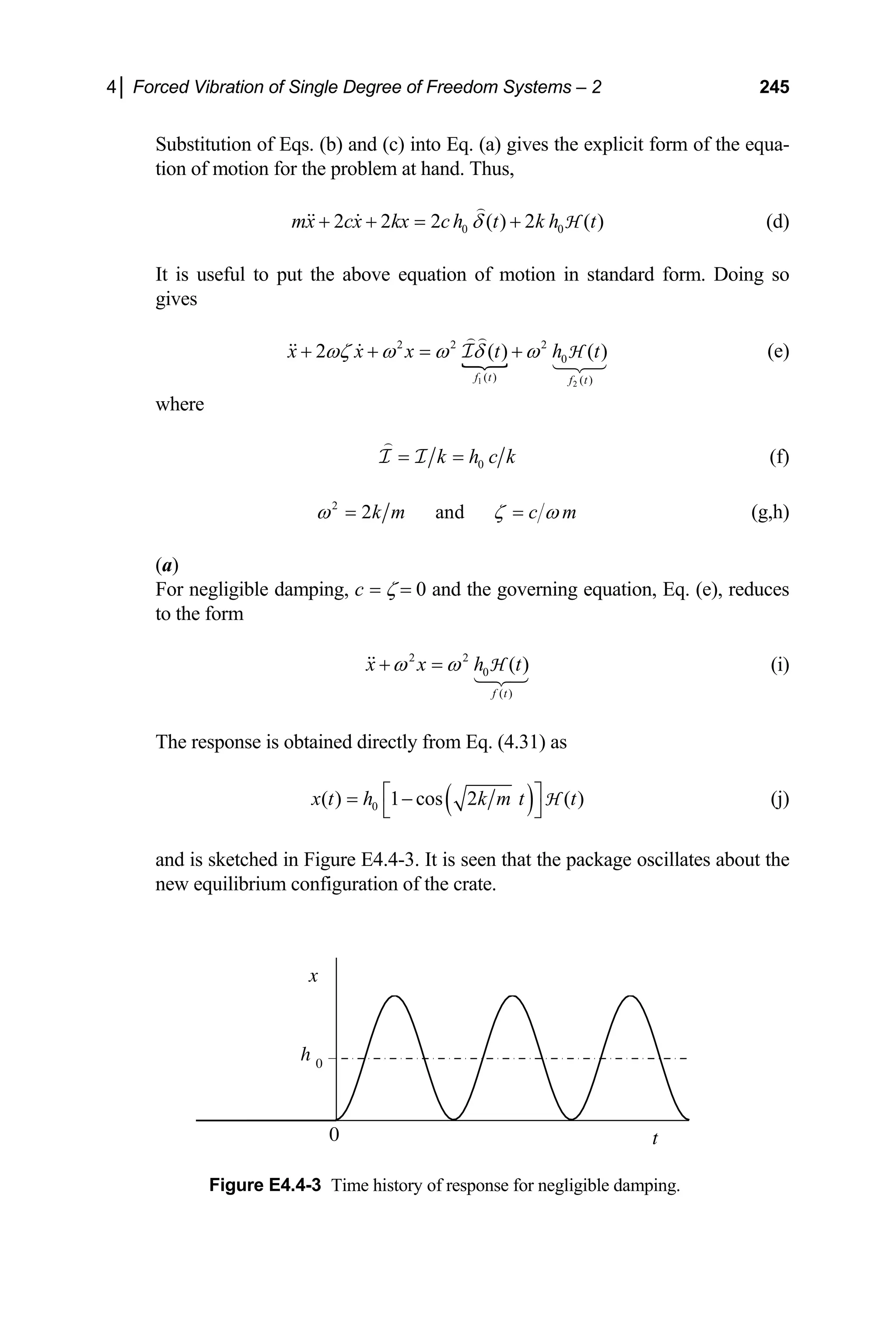
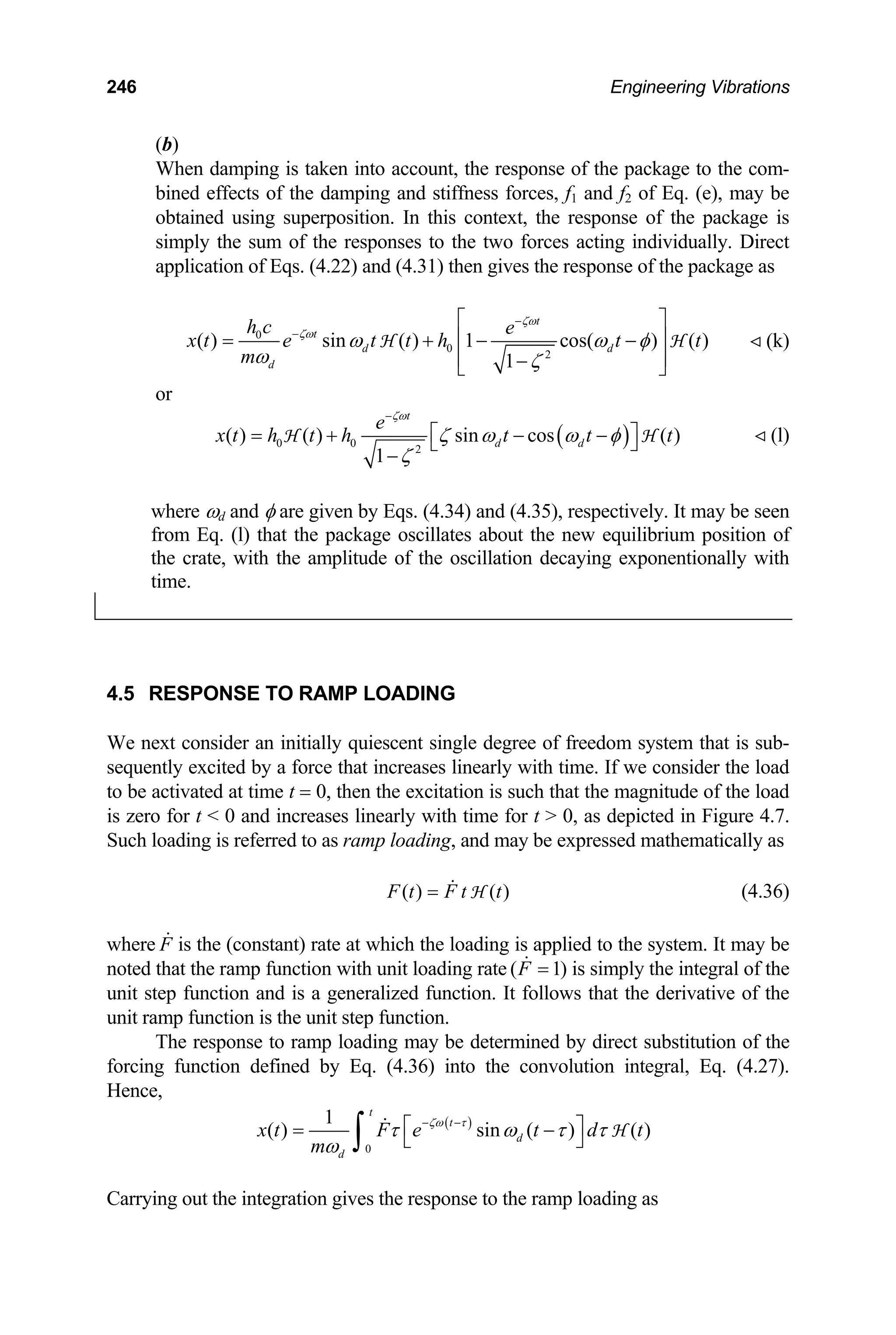
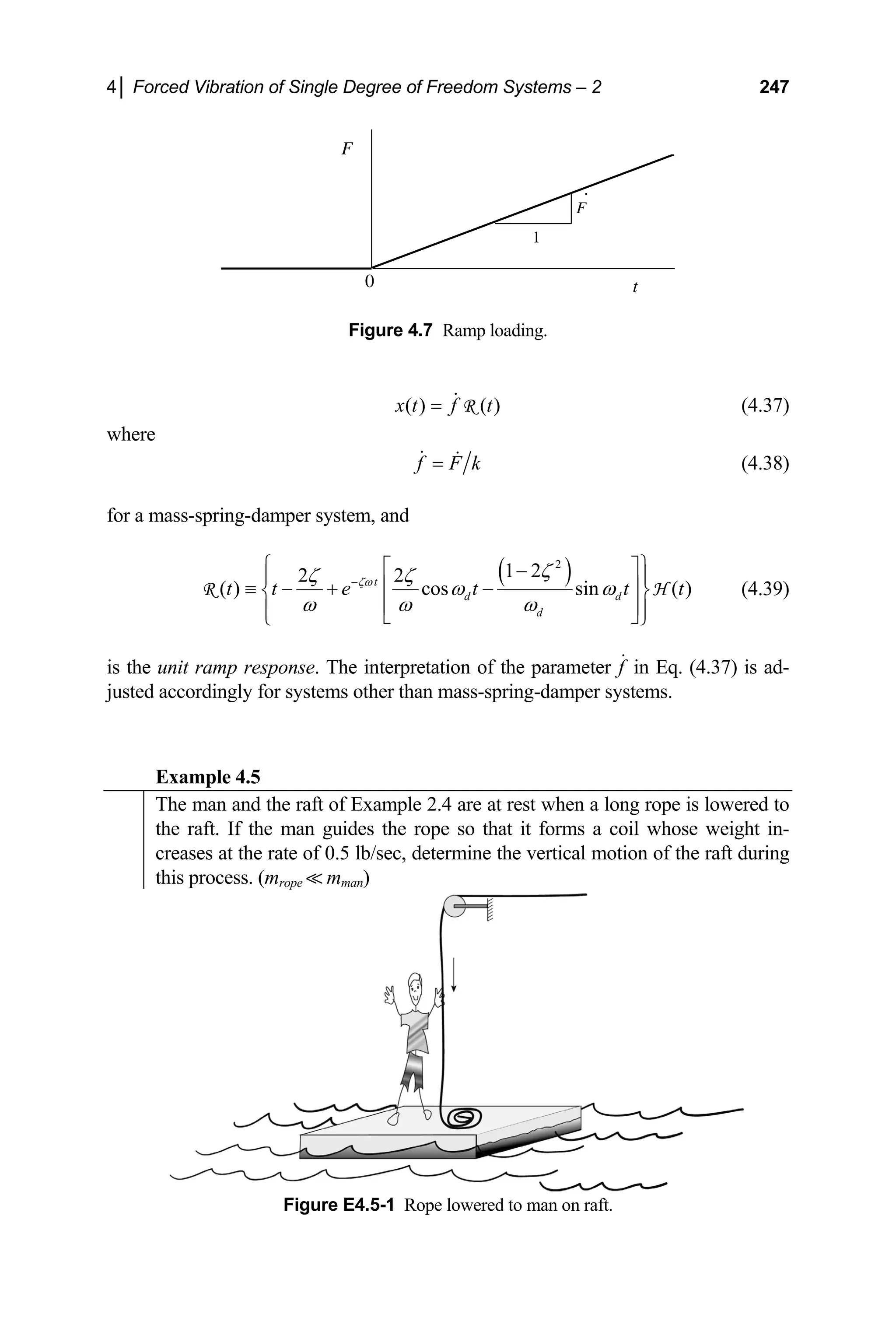
![248 Engineering Vibrations
Solution
From Example 2.4, keq = 749 lb/ft, ζ = 0 and the natural frequency of the un-
damped system is ω = 11.0 rad/sec. It is evident, from the given loading, that
the problem at hand corresponds to ramp loading of the man and raft, with
The applied force may be expressed mathematically as
0.5 lb/sec.
F =
( ) 0.5 ( )
F t t t
= H (a)
where t = 0 represents the instant that the rope first comes into contact with the
man and raft. It follows that
4
0.5
6.68 10 ft/sec
749
f −
= = × (b)
Substituting Eq. (b), ζ = 0 and ω = 11.0 rad/sec into Eqs. (4.37) and (4.39)
gives the motion of the raft during the loading process as
[ ]
4 5
1
11
( ) 6.68 10 sin(11 ) (t) 6.07 10 11 sin(11 ) (t) ft
x t t t t t
− −
= × − = × −
⎡ ⎤
⎣ ⎦ H H (c)
The time history of the response is displayed in Figure E4.5-2.
−0.5 0 0.5 1 1.5 2 2.5 3
0
10
20
30
x/A
t (secs)
Figure E4.5-2 Time history of vertical motion of man and raft as rope is lowered
.
5
( 6.07 10 ft
A −
= × )
4.6 TRANSIENT RESPONSE BY SUPERPOSITION
Many transient loads and pulses may be constructed from combinations of the basic
step and ramp functions, as well as other functions, by way of superposition. The
corresponding response is then simply the sum of the responses to the participating
functions. To demonstrate this approach, we consider the response of an equivalent
mass-spring-damper system to two basic forcing functions, the rectangular pulse and
the linear transition to constant load.](https://image.slidesharecdn.com/engineeringvibrations-240713005818-b85f16c0/75/Engineering-Vibrations-Engineering-Vibrations-270-2048.jpg)
![4│ Forced Vibration of Single Degree of Freedom Systems – 2 249
F
t
0
F0
t1
t2
Figure 4.8 The rectangular pulse.
4.6.1 The Rectangular Pulse
Consider a rectangular pulse of magnitude 0 applied to a single degree of freedom
system over the time interval 2
1
F
t
t
t
as depicted in Figure 4.8. The pulse can be
expressed as the sum of two step loads, as indicated. The pulse may thus be repre-
sented mathematically in the form
[ ]
0 1
( ) ( ) ( )
2
F t F t t t t
= − − −
H H (4.40)
From the superposition principle established in Section 3.1, the response of the sys-
tem to this pulse is then given by the sum of the responses to the individual step load-
ings. Hence, upon application of Eq. (4.31), the motion of the system is given by
[ ]
0 1 2
( ) ( ) ( )
x t f t t t t
= − − −
S S (4.41)
When expanded, Eq. (4.41) takes the form
{ }
{ }
1
2
( )
0 1
2
( )
2 2
2
( ) 1 cos ( ) ( )
1
1 cos ( ) ( )
1
t t
d
t t
d
e
1
x t f t t t t
e
t t t t
ζω
ζω
ω φ
ζ
ω φ
ζ
− −
− −
⎧⎡ ⎤
⎪
⎢ ⎥
= − − − −
⎨
⎢ ⎥
−
⎪⎣ ⎦
⎩
⎫
⎡ ⎤ ⎪
⎢ ⎥
− − − − − ⎬
⎢ ⎥
− ⎪
⎣ ⎦ ⎭
H
H
(4.42)
Thus,](https://image.slidesharecdn.com/engineeringvibrations-240713005818-b85f16c0/75/Engineering-Vibrations-Engineering-Vibrations-271-2048.jpg)
![250 Engineering Vibrations
{ }
{ }
{ }
1
2
1
1
( )
0 1
2
( )
0 2
2
( )
1 2
2
( ) 0 ( )
( ) 1 cos ( ) ( )
1
( ) cos ( )
1
cos ( ) ( )
1
t t
d
t t
d
t t
d
x t t t
e
1 2
x t f t t t t t
e
x t f t t
e
t t t t
ζω
ζω
ζω
ω φ
ζ
ω φ
ζ
ω φ
ζ
− −
− −
− −
=
⎡ ⎤
= − − −
⎢ ⎥
⎢ ⎥
−
⎣ ⎦
⎡
= − −
⎢
⎢ −
⎣
⎤
− − −
⎥
⎥
− ⎦
(4.43)
where 0 and
f φ are given by Eqs. (4.33) and (4.35), respectively.
Example 4.6
Determine the motion of the system of Example 4.3, (a) if the actuator force is
suddenly removed 10.5 seconds after first being applied to the structure, (b) if
the actuator force is suddenly removed 10 seconds after first being applied to
the structure.
Solution
(a)
For this situation, the force may be expressed as the step loading
[ ]
( ) 49.1 ( ) ( 10.5) N
F t t t
= − − −
H H (a)
The response then follows by direct application of Eqs. (4.41)–(4.43), for an
undamped system. We thus have that
[ ] [ ]
{ }
( ) 1.38 1 cos(6 ) ( ) 1 cos{6 ( 10.5)} ( 10.5) cm
x t t t t t
π π
= − − − − − −
H H (b)
Expanding equation (b) gives the motion of the system as
(c)
[ ]
[ ]
( ) 0 ( 0)
( ) 1.38 1 cos(6 ) cm (0 10.5 secs)
( ) 1.38 cos(6 ) cos{6 ( 10.5)} cm ( 10.5 secs)
x t t
x t t t
x t t t t
π
π π
=
= − − ≤
= − − ≥
It may be seen that the motion of the system between the time the force is first
applied and when it is removed is identical to that predicted in Example 4.3, as
it should be. It is also seen that, after the actuator force is removed, the system
oscillates about the original equilibrium configuration, x = 0. The time history
of the motion of the beam-block system is displayed in Figure E4.6-1.](https://image.slidesharecdn.com/engineeringvibrations-240713005818-b85f16c0/75/Engineering-Vibrations-Engineering-Vibrations-272-2048.jpg)
![4│ Forced Vibration of Single Degree of Freedom Systems – 2 251
0 5 10 15 20
−2
−1
0
1
2
x(t)
t
(cm)
(secs)
Figure E4.6-1 Time history of the motion of the beam-mass system when the actuator
force is removed 10.5 seconds after it is first applied.
(b)
The forcing function for this case may be expressed in the form
[ ]
( ) 49.1 ( ) ( 10) N
F t t t
= − − −
H H (d)
Proceeding as for the previous case yields the response
[ ] [ ]
{ }
( ) 1.38 1 cos(6 ) ( ) 1 cos{6 ( 10)} ( 10) cm
x t t t t t
π π
= − − − − − −
H H (e)
Expanding Eq. (e) gives the explicit form
(f)
[ ]
[ ]
( ) 0 ( 0)
( ) 1.38 1 cos(6 ) cm (0 10 secs)
( ) 1.38 cos{6 ( 10)} cos(6 ) 0 cm ( 10 secs)
x t t
x t t t
x t t t t
π
π π
=
= − − ≤
= − − = ≥
The time history of the motion is displayed in Figure E4.6-2. Note that, for this
case, the system comes to rest after the actuator force is removed. This is be-
cause the amplitude of the oscillation to that point corresponds to the static de-
flection due to the actuator force, and because the time between the instant the
force is first applied to the beam and the time it is removed is precisely an inte-
ger multiple of the natural period of the system. The force is therefore removed
at the exact instant that the system passes through the original equilibrium posi-
tion and is about to reverse direction. At this instant the position and velocity
are both zero. This situation is equivalent to a free vibration problem in which
the initial conditions vanish identically. The system thus remains in the equilib-
rium configuration, x = 0, for all later times.](https://image.slidesharecdn.com/engineeringvibrations-240713005818-b85f16c0/75/Engineering-Vibrations-Engineering-Vibrations-273-2048.jpg)
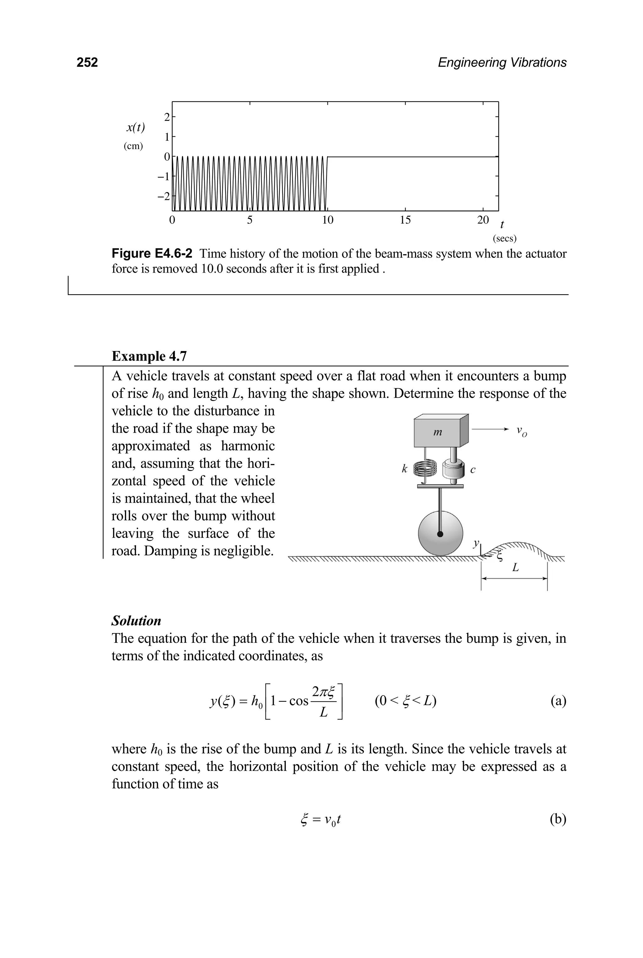
![4│ Forced Vibration of Single Degree of Freedom Systems – 2 253
where v0 is the speed and ξ is measured from the start of the bump, as indicated.
Substitution of Eq. (b) into Eq. (a) gives the vertical motion of the wheel as a
function of time. Hence,
[ ]
0
( ) 0 ( 0)
( ) 1 cos (0 )
( ) 0 ( )
L
L
y t t
y t h t t t
y t t t
=
= − Ω
=
or
[ ] ( )
[ ][ ]
0 0
0
( ) 1 cos ( ) 1 cos ( )
1 cos ( ) ( )
L L
L
y t h t t h t t t t
h t t t t
= − Ω − − Ω − −
⎡ ⎤
⎣ ⎦
= − Ω − −
H H
H H
(c)
where
2 L
t
π
Ω = (d)
and
0
L
t L v
= (e)
is the time that it takes for the vehicle to traverse the bump. The problem is thus
equivalent to that of a single degree of freedom system subjected to prescribed
motion of its support. The equation of motion is then given by Eq. (3.122)
which, for vanishing damping and support motion given by Eq. (c), takes the
form
2 2
x x y
ω ω
+ =
or
[ ] [ ]
2 2 2
0 0
( ) ( ) cos ( ) ( )
L L
x x h t t t h t t t t
ω ω ω
+ = − − − Ω − −
H H H H (f)
It may be seen from Eqs. (c) and (f) that the system is excited by the superposi-
tion of a rectangular pulse and a cosine pulse. We shall solve Eq. (f) two differ-
ent ways.
The response to the rectangular pulse is found directly from Eq. (4.42),
while the response to the cosine pulse can be evaluated using the convolution
integral, Eq. (4.27). Thus,
[ ] ( )
0 0
( ) 1 cos ( ) 1 cos ( )
L L
x t h t t h t t t t
ω ω
= − − − − −
⎡ ⎤
⎣ ⎦
H H
( )
0
0
1
cos sin ( )
t
k h t d t
m
τ ω τ τ
ω
− Ω −
∫ H
( )
0
0
1
cos sin ( )
t
L L
k h t t d t t
m
τ ω τ τ
ω
+ Ω − −
∫ H −](https://image.slidesharecdn.com/engineeringvibrations-240713005818-b85f16c0/75/Engineering-Vibrations-Engineering-Vibrations-275-2048.jpg)
![254 Engineering Vibrations
which, after carrying out the integration and using trigonometric identities and
lengthy algebraic operations, takes the form
( )
( ) ( ) ( )
2
0
2
0
( ) 1 cos cos ( )
1 cos cos ( )
L L L
x t h t t t
h t t t t
ω β ω β
ω β ω β
⎡ ⎤
= + Ω − Ω
⎣ ⎦
⎡ ⎤
− + Ω − − Ω − −
⎣ ⎦
H
H t t
(g)
where
( ) ( )
2
1 1
1 1 2 L
t
β
ω π ω
= =
− Ω −
2
(h)
Though the use of the convolution integral to obtain the response is, in
principle, straightforward it required a great deal of algebraic and trigonometric
manipulation for the current loading type. [The reader is invited to evaluate the
corresponding convolution integrals to obtain the solution (g).] An alternative,
and perhaps simpler, approach to solving Eq. (f) is to use the solutions pertain-
ing to harmonic excitation developed in Chapter 3. To do this, we shall first ob-
tain the response to the first forcing function on the right hand side of Eq. (c).
The solution to the second forcing function will then be the same as the first but
with a time shift (t replaced by t − tL). The actual response will be obtained by
superposing the two solutions.
The general solution to Eq. (f) is given by the sum of the complementary
and particular solutions. Hence, with aid of Eqs. (2.7) and (3.27), the general
form of the response (1)
( )
x t to the first forcing function
[ ]
(1)
0
( ) 1 cos ( )
f t h t t
= − Ω H is given by
[ ]
(1) (1) (1)
1 2 0
( ) cos sin 1 cos
c p
x t x x A t A t h t
ω ω β
= + = + + − Ω (i)
Imposing the quiescent initial conditions 0
)
0
(
)
0
( =
= x
x gives
( ) β
ω 2
0
1 Ω
= h
A , 0
2 =
A
Hence,
( )
2
(1)
0
( ) 1 cos cos ( )
x t h t t t
ω β ω β
⎡
= + Ω − Ω
⎣
H
⎤
⎦
(j)
The solution (2)
( )
x t associated with the second forcing function,
[ ]
(2)
0
( ) 1 cos ( ) ( )
L L
f t h t t t t
= − − Ω − −
H , is then simply given by
( )
2
(2)
0
( ) 1 cos ( ) cos ( ) ( )
L L L
x t h t t t t t t
ω β ω β
⎡ ⎤
= − + Ω − − Ω − −
⎣ ⎦
H (k)](https://image.slidesharecdn.com/engineeringvibrations-240713005818-b85f16c0/75/Engineering-Vibrations-Engineering-Vibrations-276-2048.jpg)
![4│ Forced Vibration of Single Degree of Freedom Systems – 2 255
The total response to the bump is then obtained by superposition. Hence, add-
ing Eqs. (j) and (k) gives
(1) (2)
( ) ( ) ( )
x t x t x t
= +
( )
2
0 1 cos cos
h t
ω β ω β
⎡
= + Ω − Ω
⎣
H ( )
t t
⎤
⎦
(l)
( ) ( ) ( )
2
0 1 cos cos ( )
L L L
h t t t t
ω β ω β
⎡ ⎤
− + Ω − − Ω − −
⎣ ⎦
H t t
which is identical to Eq. (g) obtained using the convolution integral. The ex-
plicit form of the response is then
( )
( ) { }
{ }
2
0
2
0
( ) 0 ( 0)
( ) 1 cos cos (0 )
( ) cos cos ( )
cos cos ( ) ( )
L
L
L L
x t t
x t h t t t t
x t h t t t
t t t t t
ω β ω β
β ω ω ω
=
⎡ ⎤
= + Ω − Ω
⎣ ⎦
⎡
= Ω − −
⎣
⎤
− Ω − Ω −
⎦
(m)
4.6.2 Linear Transition to a Constant Load Level
We next consider loading that consists of a linear transition over time τ to a constant
load level, 0 , as depicted in Figure 4.9. For this case, the loading function may be
constructed as the sum of two opposing ramp functions. Thus,
F
0 0
( ) ( ) ( ) ( )
F F
F t t t t t
τ τ
τ τ
= − −
H H − (4.44)
The response of a single degree of freedom system to this loading is then the sum of
the responses to the individual ramp functions. Hence,
[
0
( ) ( ) ( )
f
x t t t ]
τ
τ
= − −
R R (4.45)
where R (t) is given by Eq. (4.39) and, for a mass-spring-damper system,
0 0
f F k
= (4.46)
Expanding Eq. (4.45) gives the explicit form of the response of the system as](https://image.slidesharecdn.com/engineeringvibrations-240713005818-b85f16c0/75/Engineering-Vibrations-Engineering-Vibrations-277-2048.jpg)
![256 Engineering Vibrations
F
F0
t
τ
0
Figure 4.9 Linear transition to a constant level of force.
( )
( )
2
0
( )
0 0
2
( )
0
( ) 0 ( 0)
1 2
2 2
( ) cos sin (0 )
2
( ) cos cos ( )
1 2
sin sin ( ) (
t
d d
d
t t
d d
t t
d d
d
x t t
f
x t t e t t t
x t f f e t e t
f e t e t
ζω
ζω ζω τ
ζω ζω τ
ζ
ζ ζ
ω ω τ
τ ω ω ω
ζ
ω ω τ
ωτ
ζ
ω ω τ
ω τ
−
− − −
− − −
=
⎧ ⎫
⎡ ⎤
−
⎪ ⎪
⎢ ⎥
= − + −
⎨ ⎬
⎢ ⎥
⎪ ⎪
⎣ ⎦
⎩ ⎭
⎡ ⎤
= + − −
⎣ ⎦
−
⎡ ⎤
− −
⎣ ⎦ )
t
− τ
(4.47)
Example 4.8
Determine the motion of the raft of Problem 4.5 if the loading of the rope is
completed 20 seconds after the first of it touches down.
Solution
For the present problem τ = 20 seconds and, from Eq. (b) of Example 4.5,
4
0 6.68 10 ft/sec
f f
τ −
= = × 2
(a)
Substituting these values into Eqs. (4.45) and (4.47) gives the response
[ ]
{
[ ] }
5
( ) 6.07 10 11 sin(11 ) ( )
11( 20) sin11( 20) ( 20) ft
x t t t t
t t t
−
= × −
− − − − −
H
H
(b)
It is seen from Eq. (b) that during the 20 second drop of the rope, the motion of
the raft is identical to that described by Eq. (c) of Example 4.5. After the drop is
completed, that is for seconds, the vertical motion of the raft is described
by
20
t ≥
[ ]
5
( ) 0.0134 6.07 10 sin11( 20) sin(11 ) ft ( 20 secs)
x t t t t
−
= + × − − ≥ (c)](https://image.slidesharecdn.com/engineeringvibrations-240713005818-b85f16c0/75/Engineering-Vibrations-Engineering-Vibrations-278-2048.jpg)
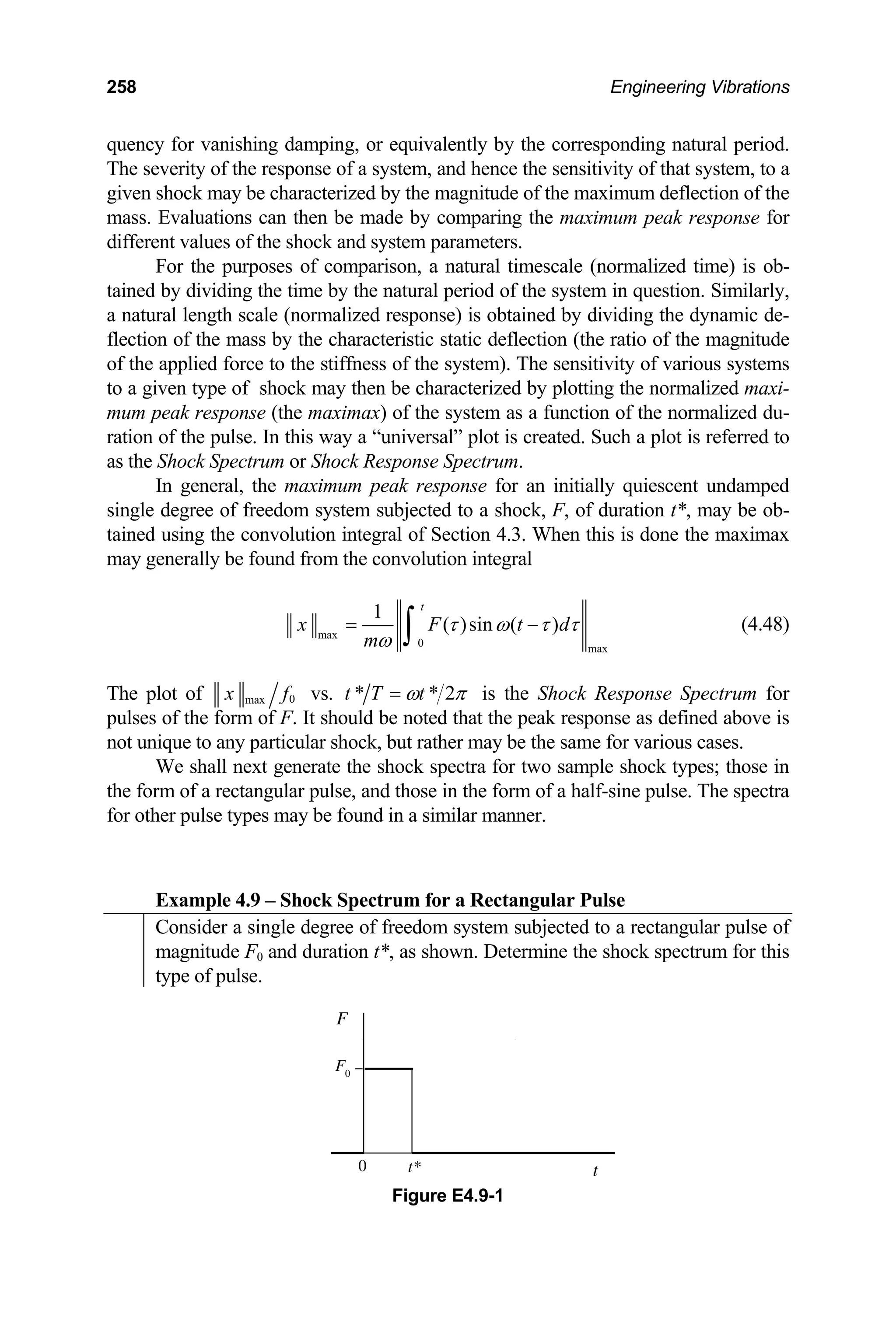
![4│ Forced Vibration of Single Degree of Freedom Systems – 2 259
Solution
The response of a single degree of freedom system to a rectangular pulse was
established in Section 4.6.1. If we neglect the effects of damping, the response
of the system to the rectangular pulse is obtained from Eq. (4.43) as
)
0
(
0
)
(
= t
t
x (a)
[ ]
0
( ) 1 cos (0 *)
x t f t t t
ω
= − ≤ (b)
[ ] *)
(
cos
*)
(
cos
)
( 0 t
t
t
t
t
f
t
x
−
−
= ω
ω (c)
where 2 T
ω π
= is the natural frequency of the system and T is the correspond-
ing natural period. The peak response may occur either (i) during the time in-
terval that the applied pulse is active (0 t t*), or (ii) after the pulse subsides
(t t*).
(i) 0 t t* : Initial Spectrum
The maximum response of the system, while the applied pulse is active is de-
termined by consideration of Eq. (b). For short duration pulses ( * 0.5 )
t T
it is
seen from Eq. (b) that
2
max
0
1 cos * 2sin ( * ) ( * 0.5 )
x
t t T t
f
ω π
= − = T
T
(d-1)
For long duration pulses , it is seen that
( * 0.5 )
t ≥
max
0
2 ( * 0.5 )
x
t T
f
= (d-2)
It may be seen from Eqs. (d-1) and (d-2) that the initial shock spectrum for the
rectangular pulse increases monotonically as the duration of the pulse in-
creases, and reaches a plateau when the duration of the pulse is at least half the
natural period of the system (Figure E4.9-2).
(ii) : Residual Spectrum
*
t t
We next consider the maximum response achieved by the system after the
pulse subsides. To find the time (t = tpk) at which the peak response occurs for
this case, and hence to find the peak response when t t*, we take the deriva-
tive of Eq. (c), set it to zero and solve for the time. Hence,](https://image.slidesharecdn.com/engineeringvibrations-240713005818-b85f16c0/75/Engineering-Vibrations-Engineering-Vibrations-281-2048.jpg)
![260 Engineering Vibrations
[ pk
pk
t
t
t
t
t
t
t
f
dt
dx
=
=
−
−
−
=
= ω
ω
ω sin
*)
(
sin
0 0 ] (e)
With the aid of the identity sin(a) – sin(b) = 2 cos{(a + b)/2} sin{(a − b)/2},
Eq. (e) takes the form
{ } { }
1 1
2 2
2cos (2 *) cos * 0
pk
t t t
ω ω
− = (f)
Hence,
*
(2 1)
2 2
pk
t
t n
ω π
ω = + − (g)
Evaluating Eq. (c) at t = tpk and substituting Eq. (g) into the resulting expression
gives the maximum response
max
0
*
2sin
x t
f T
π
⎛ ⎞
= ⎜ ⎟
⎝ ⎠
(h)
A plot of Eq. (h) (the residual shock spectrum) is displayed in Figure 4.9-2
along with the initial shock spectrum described by Eq. (d). It may be seen that
the maximum displacements are larger and hence the residual spectrum domi-
nates for short duration pulses while the initial spectrum dominates for large
duration pulses. It may also be seen that the most sensitive systems are those
for which the duration of the pulse is at least as large as half the natural period
of the system (i.e., those for which 5
.
0
* ≥
T
t ). The complete shock spectrum
is indicated by solid lines in Figure E4.9-2.
0 0.5 1 1.5 2 2.5 3
0
0.5
1
1.5
2
t*/T
initial
spectrum
residual
spectrum
x max
Figure E4.9-2 Shock spectrum for a rectangular pulse.](https://image.slidesharecdn.com/engineeringvibrations-240713005818-b85f16c0/75/Engineering-Vibrations-Engineering-Vibrations-282-2048.jpg)
![4│ Forced Vibration of Single Degree of Freedom Systems – 2 261
Example 4.10 – Response Spectrum for Rectangular Support Motion
Determine the shock spectrum for a single degree of freedom system when the
time history of the motion of the support is in the form of a rectangular pulse of
amplitude h0 and duration t*.
x
t
0
h 0
t*
F
Figure E4.10-1
Solution
The motion of the support shown in Figure E4.10-1 may be expressed in the
form
[ ]
0
( ) ( ) ( *)
F
x t h t t t
= − −
H H (a)
Substitution of Eq. (a) into Eq. (3.122) gives the equation governing absolute
motion as
[ ]
2 2
0 ( ) ( *)
x x h t t t
ω ω
+ = − −
H H (b)
Thus, the present problem is identical in form with that of Example 4.9, with f0
replaced by h0. The absolute motion of the mass then follows from Eq. (4.43)
or Eqs. (a)–(c) of Example 4.9 with f0 replaced by h0. For the present problem,
the extension/compression of the equivalent elastic spring is described by the
motion of the mass relative to the support,
( ) ( ) ( )
F
u t x t x t
= − (c)
Hence,
( ) ( ) 0 ( 0)
u t x t t
= = (d)
0
( ) cos (0 *)
u t h t t t
ω
= − ≤ (e)
[ ]
0
( ) ( ) cos ( *) cos ( *)
u t x t h t t t t t
ω ω
= = − − − (f)
We see from Eq. (e) that the maximum relative deflection of the mass while the
pulse is active is](https://image.slidesharecdn.com/engineeringvibrations-240713005818-b85f16c0/75/Engineering-Vibrations-Engineering-Vibrations-283-2048.jpg)
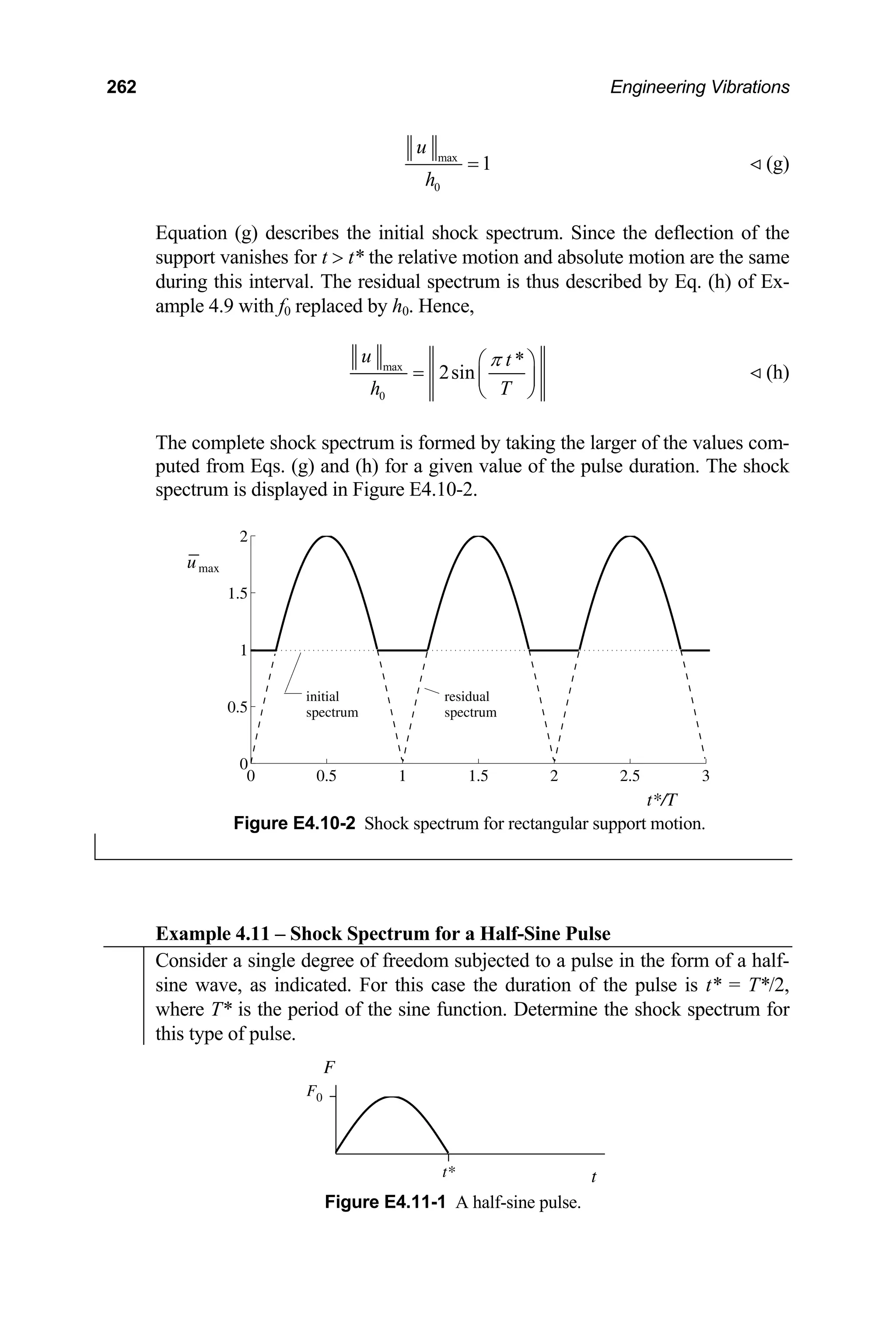
![4│ Forced Vibration of Single Degree of Freedom Systems – 2 263
t
F
F0
t*
Figure E4.11-2 Pulse represented as superposition of sine waves.
Solution
The forcing function for this pulse takes the form
[ ]
0
0 0
( ) sin ( ) ( *)
sin ( ) sin ( *) ( *)
F t F t t t t
F t t F t t t t
= Ω − −
= Ω + Ω − −
H H
H H
(a)
where
2 * /
T *
t
π π
Ω = = (b)
(see Figure E4.11-2). Substitution of Eq. (a) into Eq. (4.48) gives
0
0
0
0
( ) sin sin ( ) ( )
sin ( *) sin ( * ) ( *)
t
t
F
x t t d t
m
F
t t t d t
m
τ ω τ τ
ω
τ ω τ τ
ω
= Ω −
+ Ω − + −
∫
∫
H
H t
−
(c)
Carrying through the integration gives the response to the half-sine pulse as
( )
( )
{ }
2
0
( ) 1
sin * sin ( )
2 *
1 2 *
sin ( *) * sin ( *) ( *)
2 *
x t T
t t t t
f t
T t
T
t t t t t t t
t
π ω
π ω
⎧⎡ ⎤
= −
⎨⎢ ⎥
⎣ ⎦
− ⎩
⎫
⎡ ⎤
+ − − − − ⎬
⎢ ⎥
⎣ ⎦ ⎭
H
H
(d)
We must next determine the maximum values of the response and when they
occur. We shall consider two intervals, (i) the time interval during which the
pulse is still active (t t*) and (ii) the interval after the pulse subsides (t t*).
The maximum displacements will then be plotted as a function of the duration
of the pulse, constructing the shock spectrum for the half-sine pulse.](https://image.slidesharecdn.com/engineeringvibrations-240713005818-b85f16c0/75/Engineering-Vibrations-Engineering-Vibrations-285-2048.jpg)
![4│ Forced Vibration of Single Degree of Freedom Systems – 2 265
Similarly, substituting Eq. (h-2) into Eq. (e) and noting that
( ) 2 2
2 2
b
pk
n n
t n n
π ω π
ω π π
ω ω
Ω
+ = + =
Ω − Ω −
gives the second set of extrema as
( )
( )
( )
0
1
sin
1
b
pk
b
pk
t t
x f
ω
=
=
⎡ ⎤
+ Ω
⎣ ⎦
t
Ω (j)
It may be seen by comparing Eqs. (i) and (j) that
( ) ( )
a b
pk pk
t t t t
x x
= =
and hence that
( )
max a
pk
t t
x x =
= (k)
Substituting Eqs. (h-1) and (i) into Eq. (e) gives the maximum response during
the interval for which the pulse is active as
( ) ( )
max
0
1 2
sin
1 2 *
1 2 *
x n
f t
T t
π
T
⎧ ⎫
⎪ ⎪
= ⎨ ⎬
+
⎡ ⎤
− ⎪ ⎪
⎩ ⎭
⎣ ⎦
(l)
where tpk t* and, from Eq. (h-1),
1 *
2
t
n
T
+ (m)
Since n must be an integer, it is seen from Eq. (m) that no maxima occur when
the duration of the pulse is less than half the natural period of the system.
(ii) t t* : Residual Spectrum
Evaluating Eq. (e) for t t* gives the response of the system after the pulse has
subsided as
( )
[
2
0
( ) 2 *
sin sin ( *)
2 * 1
x t T t
t t t
f T t
ω ω
= +
⎡ ⎤
−
⎣ ⎦
]
− (n)
Differentiating Eq. (n) and setting the resulting expression to zero gives](https://image.slidesharecdn.com/engineeringvibrations-240713005818-b85f16c0/75/Engineering-Vibrations-Engineering-Vibrations-287-2048.jpg)
![266 Engineering Vibrations
[ ]
cos cos ( *) 0
pk
t t
t t t
ω ω =
+ − =
which, after using the identity cos(a) + cos(b) = 2cos{(a + b)/2}cos{(a − b)/2},
takes the alternate form
( )
{ } { }
1 1
2 2
cos * cos * 0
t t t
ω ω
− = (o)
It follows that
*
(2 1)
2 2
pk
t
t n
ω π
ω = + − (p)
Substituting Eq. (p) into Eq. (n) gives the maximum response after the pulse
has subsided as
( )
( )
( )
max
2
0
2 *
2 cos
2 * 1
x t T
t T
f t T
π
=
⎡ ⎤
−
⎣ ⎦
* (q)
A plot of the residual spectrum is displayed in Figure E4.11-3, along with the
initial spectrum. For a given range of the pulse duration ratio t*/T, the greater
of the initial or residual maxima form the shock spectrum. It may be seen that
the residual spectrum dominates when the duration of the pulse is less than half
the natural period of the system while the initial spectrum governs for t* T / 2
0 0.5 1 1.5 2 2.5 3 3.5 4
0
0.5
1
1.5
2
xmax
t*/T
n = 1
n = 2
n = 3
n = 4
residual
Figure E4.11-3 Shock spectrum for a half-sine pulse.](https://image.slidesharecdn.com/engineeringvibrations-240713005818-b85f16c0/75/Engineering-Vibrations-Engineering-Vibrations-288-2048.jpg)
![4│ Forced Vibration of Single Degree of Freedom Systems – 2 267
Example 4.12 – Motion of the Support in Form of a Half-Sine Wave
Consider a shock in the form of a sudden motion of the support of a mass-
spring-damper system (such as in Example 4.10). Set up the equations that de-
scribe the shock spectrum of the system if the time history of the displacement
of the support is in the form of a half-sine pulse.
Solution
The motion of the support is of the form
0
0 ( 0)
( ) sin (0 *)
0 ( *)
F
t
x t h t t t
t t
⎧
⎪
= Ω
⎨
⎪
⎩
(a)
where
2 * /
T *
t
π π
Ω = = (b)
The motion can be described formally by the equation
[ ]
[ ]
0
0
( ) sin ( ) ( *)
sin ( ) sin ( *) ( *)
F
x t h t t t t
h t t t t t t
= Ω − −
= Ω + Ω − −
H H
H H
(a')
The equation that governs the absolute motion of the mass is, from Eq. (3.122),
( ) ( ) ( )
F
m x t k x t k x t
+ = (c)
(i) 0 t t* : Initial Spectrum
During the interval that the pulse is active the equation of motion takes the
form
0
( ) ( ) sin
m x t k x t kh t
+ = Ω (d)
The absolute response may be determined directly from Eq. (e) of Example
4.11 by letting F0 = kh0. Hence,
( )
( )
2
0
( ) 1
sin * sin
2 *
1 2 *
x t T
t t t
h t
T t
π ω
⎡ ⎤
= −
⎢ ⎥
⎣ ⎦
−
(e)
The relative displacement of the mass with respect to the support is then
( )
( )
( ) ( )
2
0 0
2 *
( ) ( )
( )
2 * sin * sin
1 2 *
F
T t
x t x t
u t
T t t t t
h h T t
π ω
−
⎡ ⎤
= = −
⎣ ⎦
−
(f)](https://image.slidesharecdn.com/engineeringvibrations-240713005818-b85f16c0/75/Engineering-Vibrations-Engineering-Vibrations-289-2048.jpg)
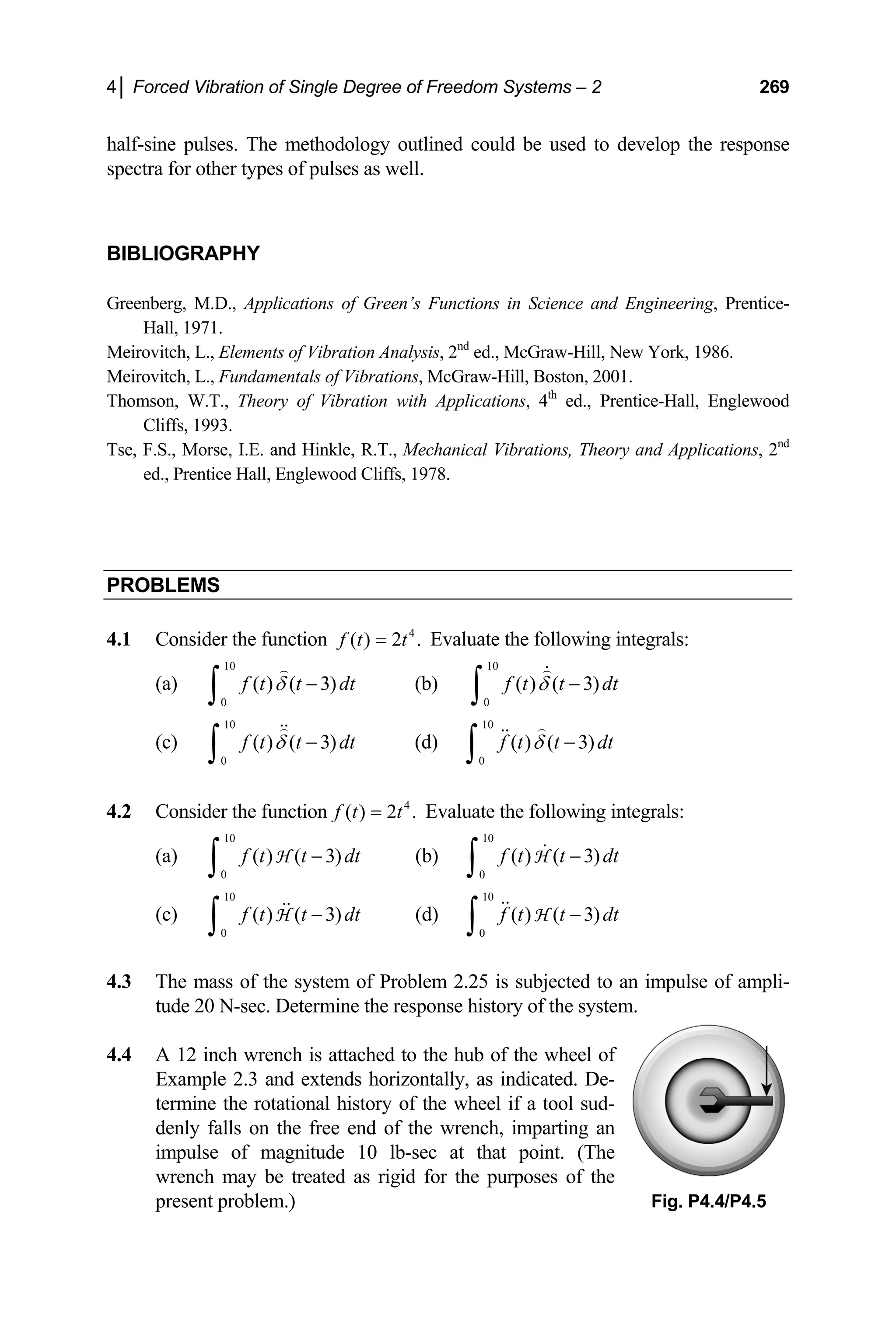
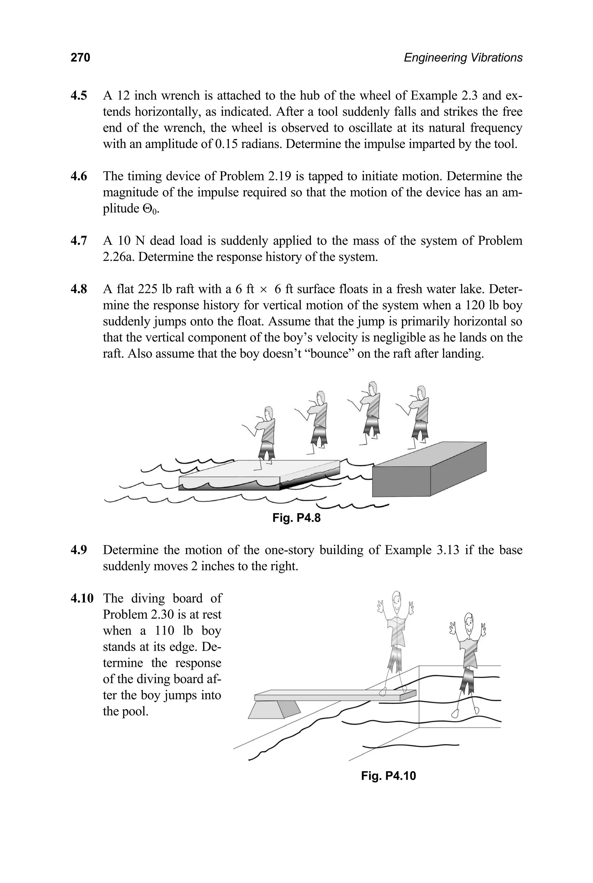
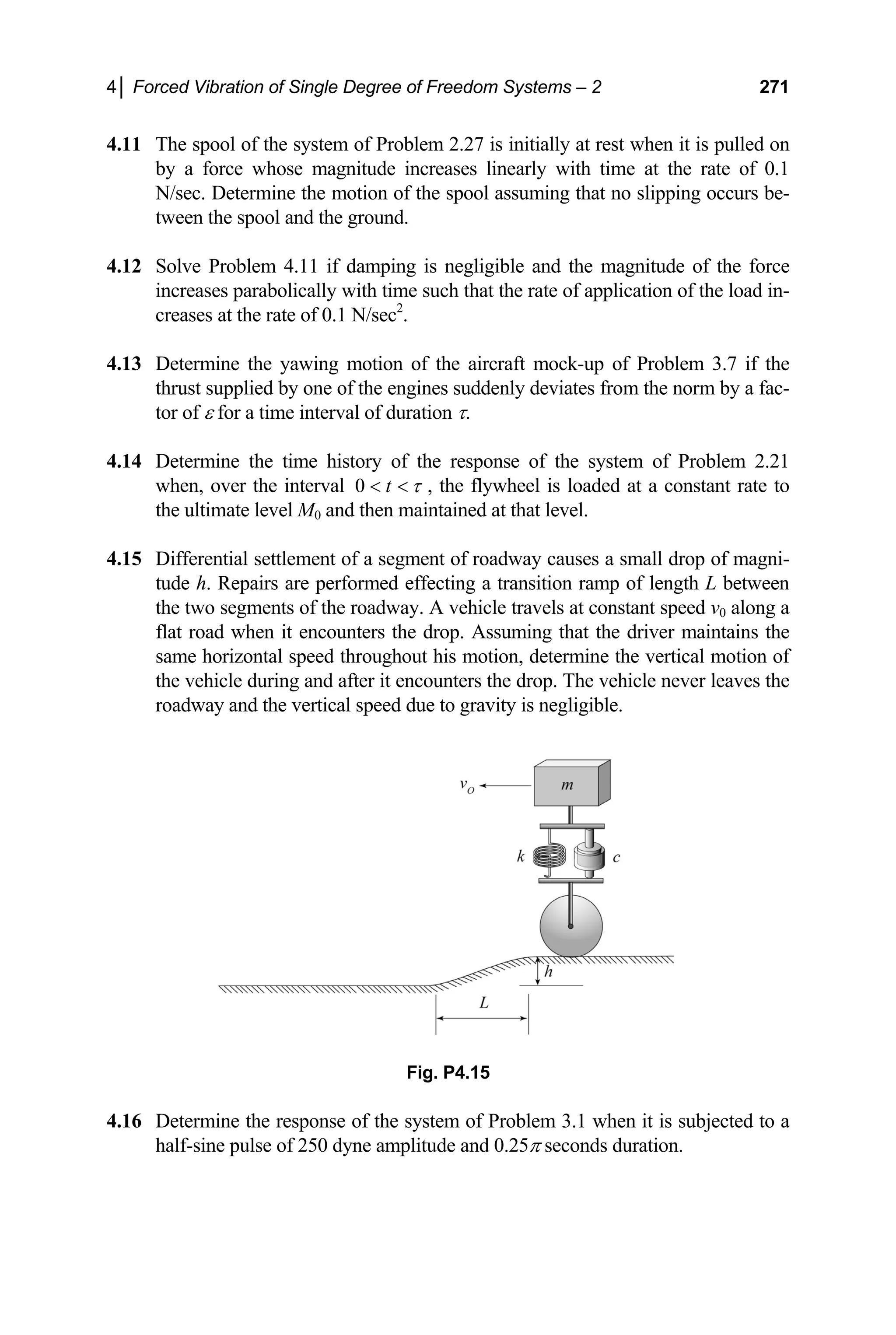
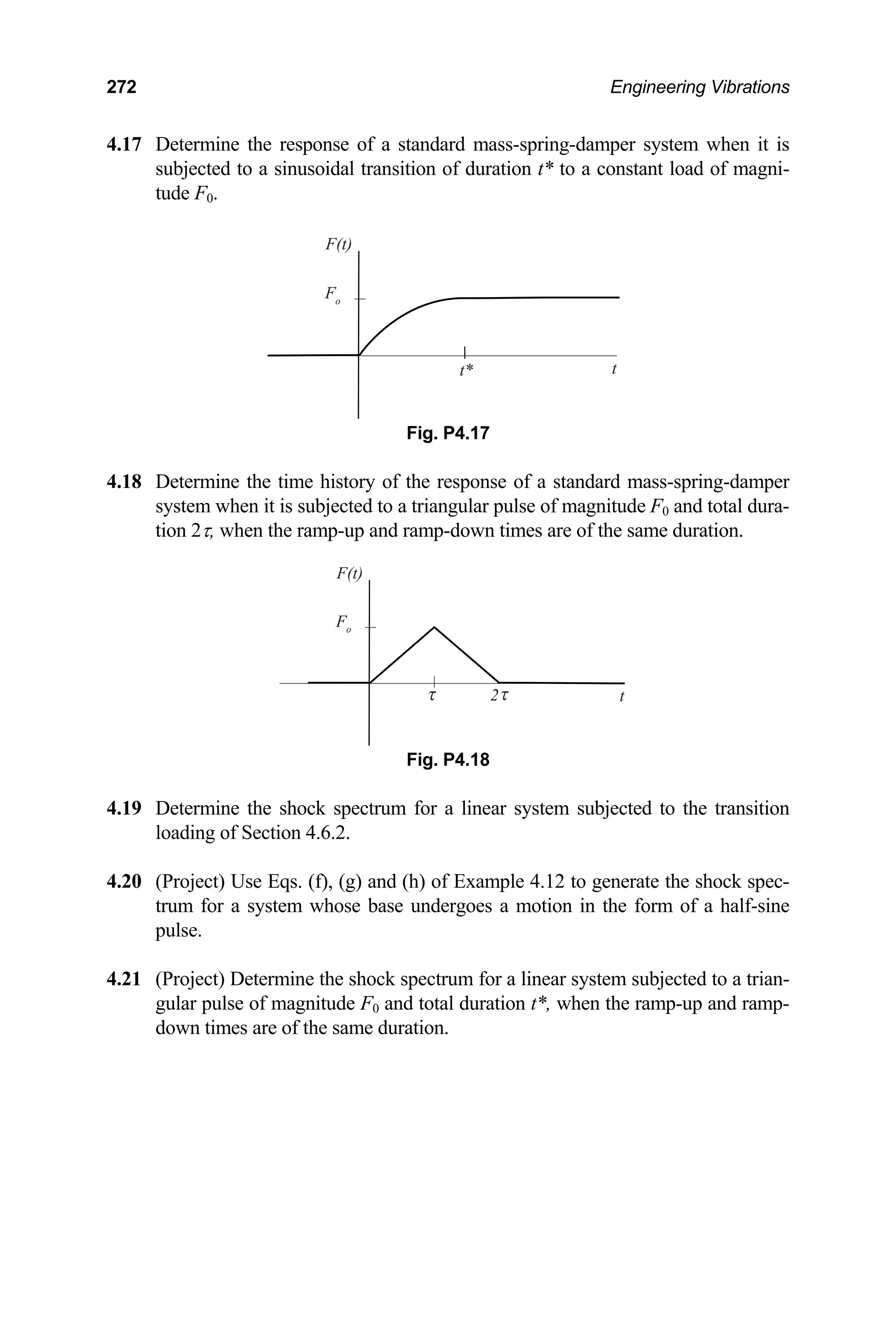
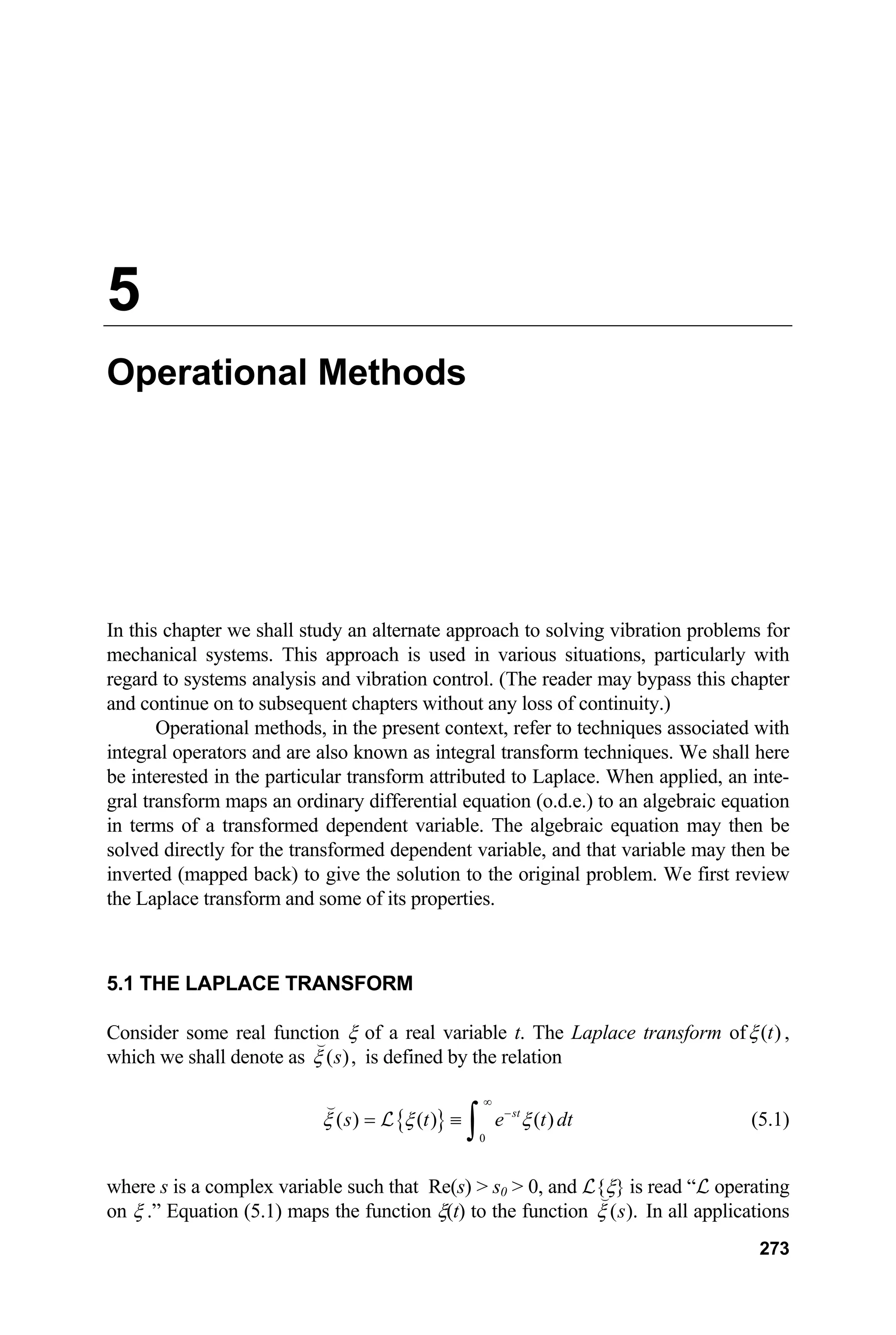
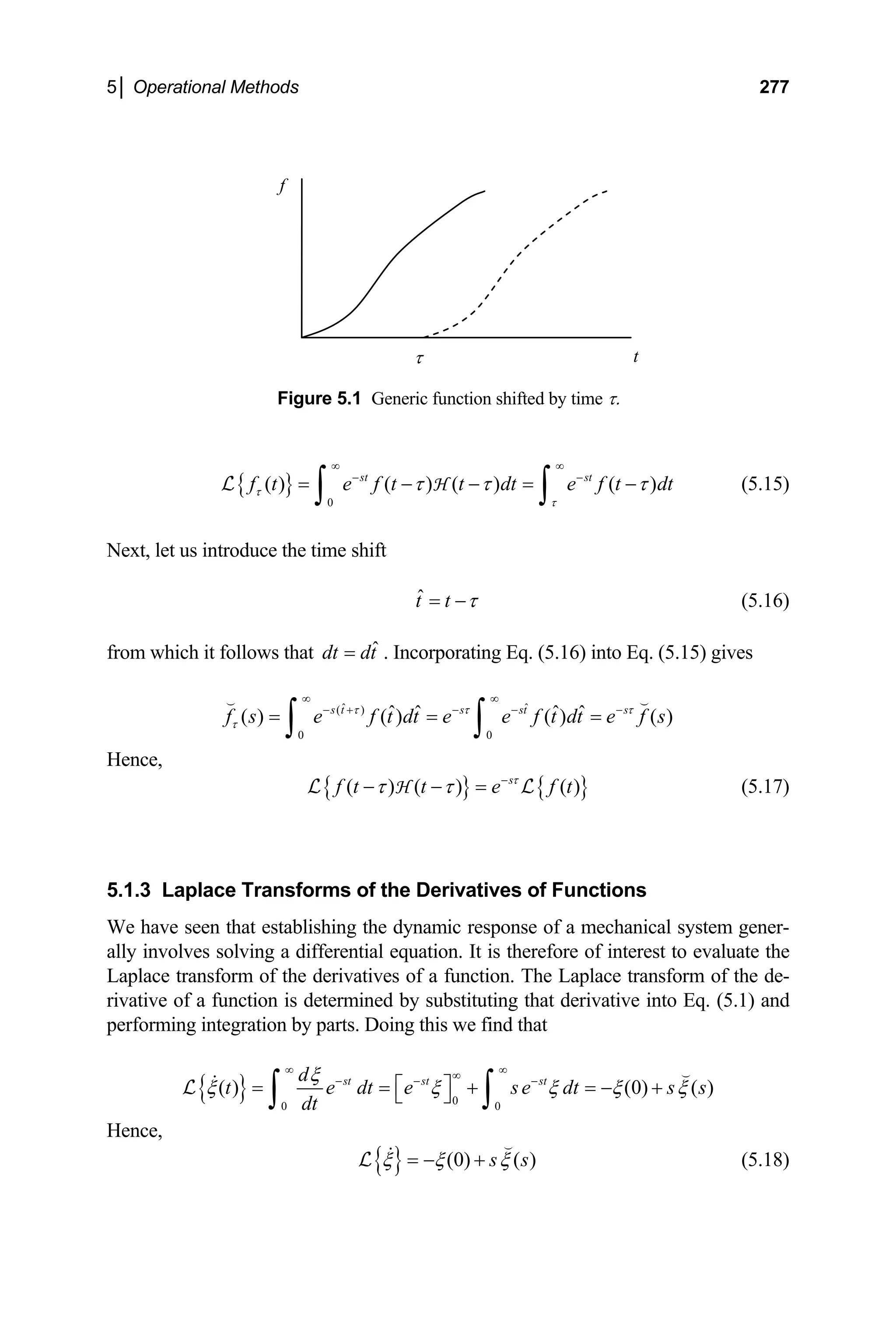
![280 Engineering Vibrations
Taking the Laplace transform of the governing equation, exploiting the property that
Laplace transformation is a linear operation and using Eqs. (5.18) and (5.19), results
in the algebraic equation for the transformed displacement
[ ]
2 2
(0) (0) ( ) 2 (0) ( ) ( ) 0
x s x s x s x s x s x s
ωζ ω
⎡ ⎤
− − + + − + + =
⎣ ⎦
(5.25)
Equation (5.25) may be solved for ( )
x s
to give
( )
0
2
2
( )
2
v s x
x s
s s
ωζ 0
2
ωζ ω
+ +
=
+ +
(5.26)
If we compare the denominator of Eq. (5.26) with the characteristic function Z(s),
the left-hand side of Eq. (2.67), it is seen that the denominator corresponds to the
characteristic function. Further, let us recall that the roots of the characteristic equa-
tion Z(s) = 0 yield the exponents of Eq. (2.66) and hence the general form of the solu-
tion. Let us next factor the denominator of Eq. (5.26) to give the form
( )
( ) ( )
0 0
2
( )
d d
v s x
x s
s i s i
ωζ
ζω ω ζω ω
+ +
=
+ + + −
⎡ ⎤ ⎡ ⎤
⎣ ⎦ ⎣ ⎦
(5.27)
where ωd is defined by Eq. (2.70) for underdamped systems. It may be seen that the
singularities of the transformed displacement, the values of s for which the bracketed
expressions in the denominator of Eq. (5.27) vanish, correspond to the roots of the
characteristic equation Z(s) = 0. In order to invert the transformed displacement, and
hence to obtain the response x(t), it is desirable to express Eq. (5.27) in a form, or
combination of forms, that corresponds to the Laplace transform of functions that we
have already established or are listed elsewhere. This may be accomplished by multi-
plying the respective factors in the denominator back again, and regrouping terms.
The transformed displacement then takes the form
( )
( )
( )
( )
0 0
0 2 2 2
2
( )
1
d d
s v x
x s x
s s
ζω ω ζ ω
2
ζω ω ζω ω
ζ
+
= +
+ + + +
−
(5.28)
Equation (5.28) may now be inverted by direct application of Eqs. (5.12) and (5.13).
This gives the free vibration response as
{ }
( )
0 0
1
0
2
( ) ( ) cos sin
1
t t
d d
v x
x t x s x e t e
ζω ζω
ω ζ
t
ω ω
ζ
− − −
⎡ ⎤
+
= = + ⎢ ⎥
⎢ ⎥
−
⎣ ⎦
L (5.29)
Substituting Eqs. (2.6)–(2.11) puts the response in the form identical to Eq. (2.74).](https://image.slidesharecdn.com/engineeringvibrations-240713005818-b85f16c0/75/Engineering-Vibrations-Engineering-Vibrations-302-2048.jpg)
![282 Engineering Vibrations
( )
x s
( )
f s
Q(s)
Figure 5.2 Block diagram for forced vibration problem.
is referred to as the mechanical admittance (transfer function) and, in the present con-
text, is seen to correspond to the displacement per unit (specific) force in the trans-
formed space. From a systems perspective, ( )
f s
and ( )
x s
may be viewed as input-
output pairs, with Q(s) the corresponding transfer function as depicted in the block
diagram of Figure 5.2. Both Z(s) and Q(s) characterize the system and are important
parameters in certain applications (such as control theory).
5.3.2 Steady State Response
Let us next consider the response of single degree of freedom systems to external
time dependent forces. In particular, let us first consider the response to harmonic
forcing. Thus, let us consider the external force of the form
[ ]
0 0
( ) cos sin
i t
f t f e f t i t
Ω
= = Ω + Ω (5.37)
It follows from Eq. (5.8), or equivalently from Eqs. (5.10) and (5.11), that
0
( )
f
f s
s i
=
− Ω
(5.38)
The transform of the response is then readily obtained by substituting Eq. (5.38) into
Eq. (5.34). This gives
2 2
0 0 0 0
2 2 2 2
( ) ( )
( )
( )( 2 ) ( ) ( ) d
f s f s
x s
s i s s s i s
ω ω
ωζ ω ζω ω
+ +
= =
− Ω + + ⎡ ⎤
− Ω + +
⎣ ⎦
Z Z
(5.39)
The physical response is found by inverting Eq. (5.39). This can be done by expand-
ing the denominator and using partial fractions. However, it is expedient as well as
instructive to perform the inversion using the convolution theorem. To do this we first
partition Eq. (5.39) using Eqs. (5.8), (5.12) and (5.13). We then incorporate the result-
ing expression into Eq. (5.23) to get
{ }
1 2 ( )
0
0
( ) ( ) sin ( )
t
i t
d a
x t x s f e e x
τ ζωτ
d
ω ω τ τ τ
− Ω − −
⎡ ⎤
= = +
⎣ ⎦
∫
L (5.40)](https://image.slidesharecdn.com/engineeringvibrations-240713005818-b85f16c0/75/Engineering-Vibrations-Engineering-Vibrations-304-2048.jpg)
![5│ Operational Methods 283
where xa(t) is given by Eq. (5.29). Evaluating the integral in Eq. (5.40) gives the re-
sponse of the system as
( )
[
0
2
( ) ( ) ( )
1 2
i t
t
a b
f e
]
x t e x
i
ζω
ζ
Ω
−
= +
− Ω + Ω
t x t
+ (5.41)
where
ω
Ω ≡ Ω (5.42)
( )
2 2
2
( ) 1 2 cos sin
1
a d
i
d
x t i t
ζ
ζ ω ω
ζ
t
⎡ ⎤
+ Ω
⎡ ⎤ ⎢ ⎥
= Γ − Ω − Ω +
⎣ ⎦ ⎢ ⎥
−
⎣ ⎦
(5.43)
( )
0 0
2
( ) cos sin
1
b d
v x
d
x t t
ω ζ
t
ω ω
ζ
+
= +
−
(5.44)
and Γ is given by Eq. (3.50). The second term in Eq. (5.41) may be seen to tend to
zero for large t, and thus will become negligible after sufficient time has elapsed fol-
lowing the start-up of the system. Therefore, neglecting the decaying term in that
expression gives the steady state response as
( ) (
0
( ) ; i t
ss
x t f e
ζ )
Ω −Φ
= Γ Ω (5.45)
where Γ and Φ respectively correspond to the magnification factor and phase angle
of the steady state response, as discussed in Section 3.3.3. The response given by Eq.
(5.45) is seen to be identical with that described by Eq. (3.52) as, of course, it should
be.
5.3.3 Transient Response
We next consider the response of initially quiescent systems to short duration loads
(pulses). It is seen from Eq. (5.33) that Z0 = 0 for systems that are initially at rest.
Impulse Response
Consider a single degree of free system, say a mass-spring-damper system that is
subjected to an impulse of the form
( ) ( )
f t t
k
δ
=
I
(5.46)](https://image.slidesharecdn.com/engineeringvibrations-240713005818-b85f16c0/75/Engineering-Vibrations-Engineering-Vibrations-305-2048.jpg)
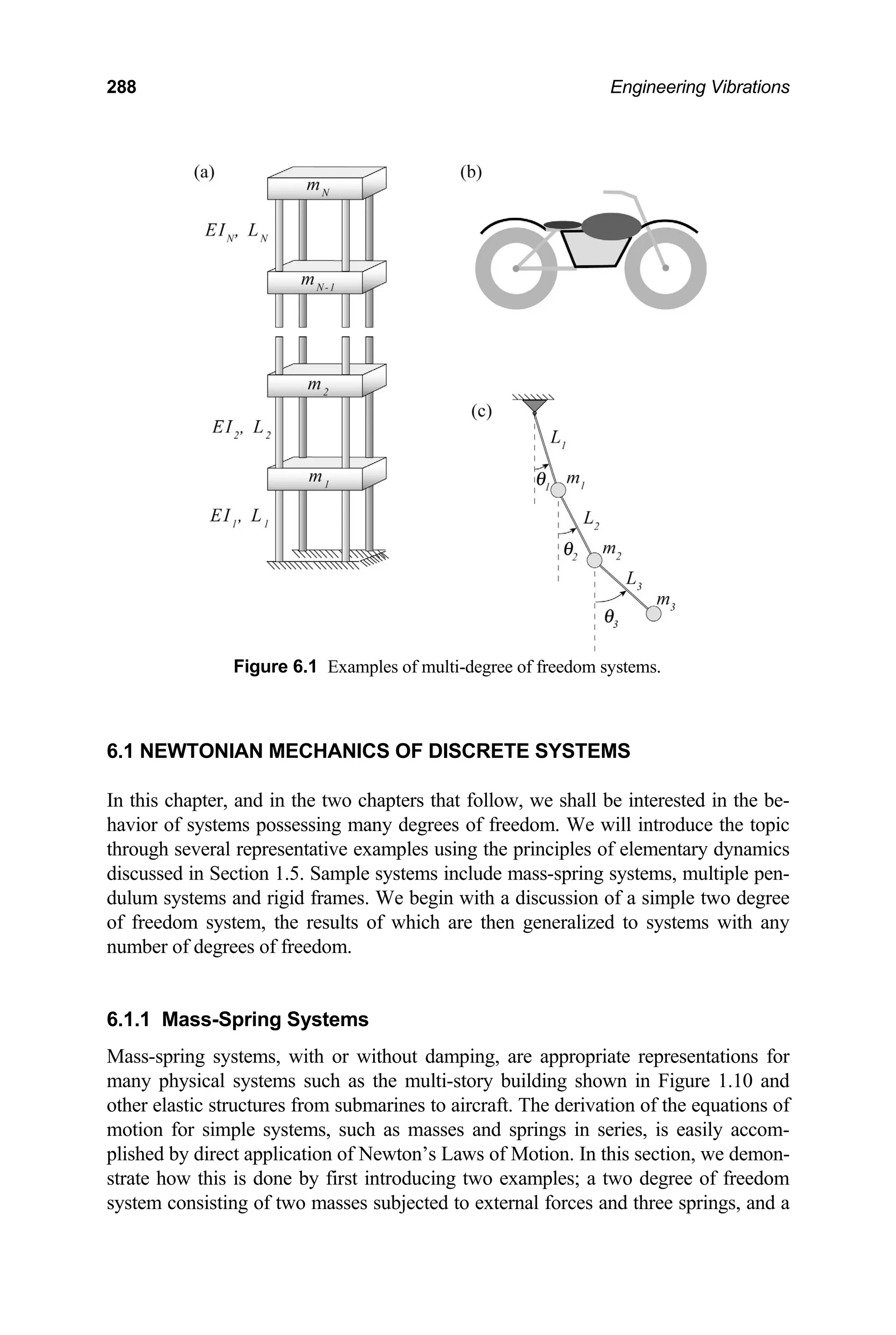
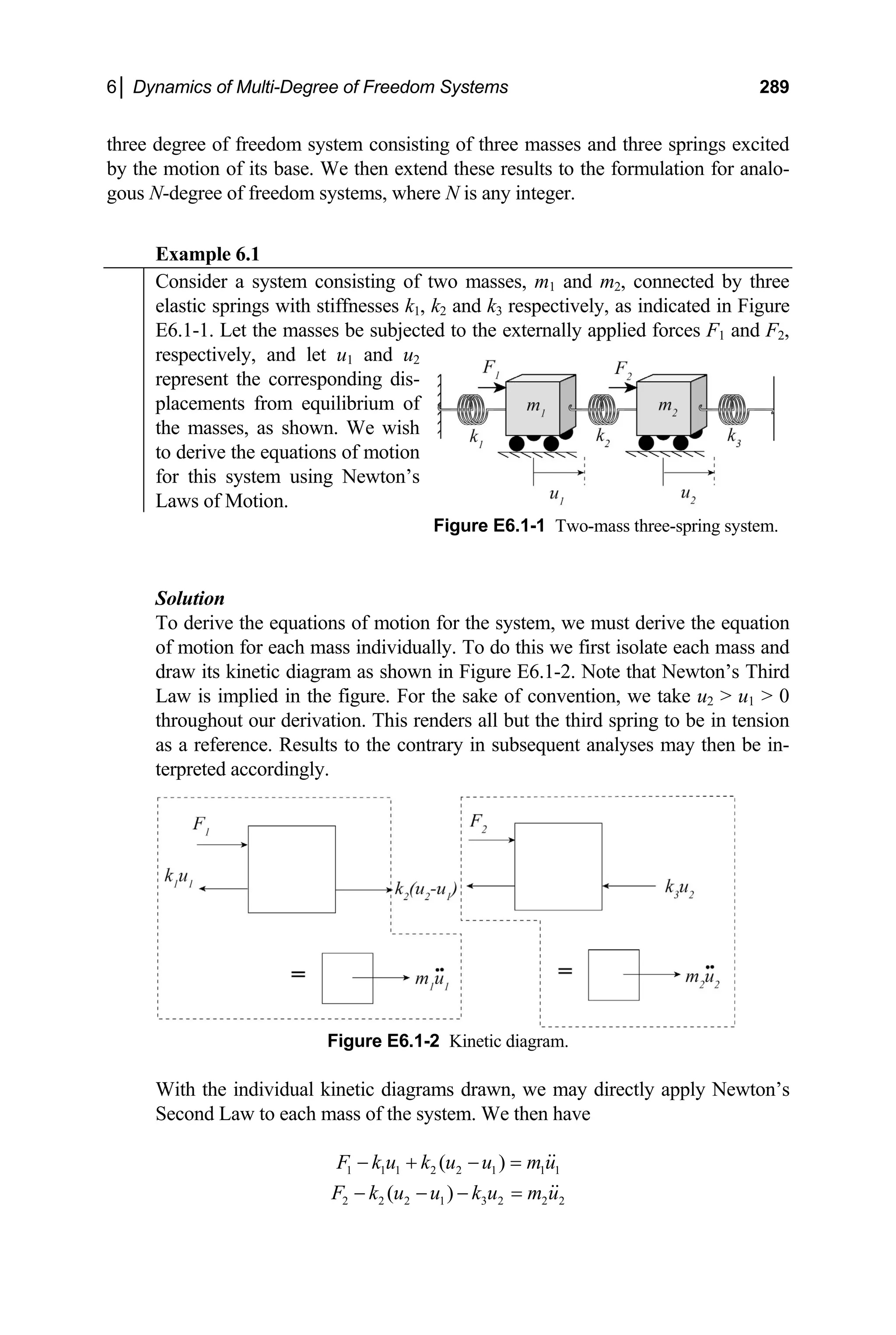
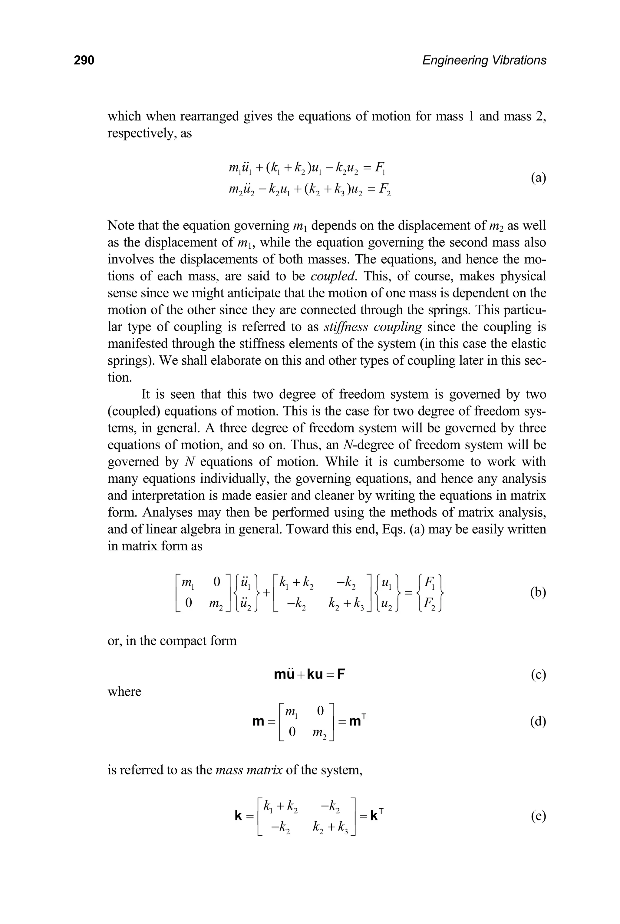
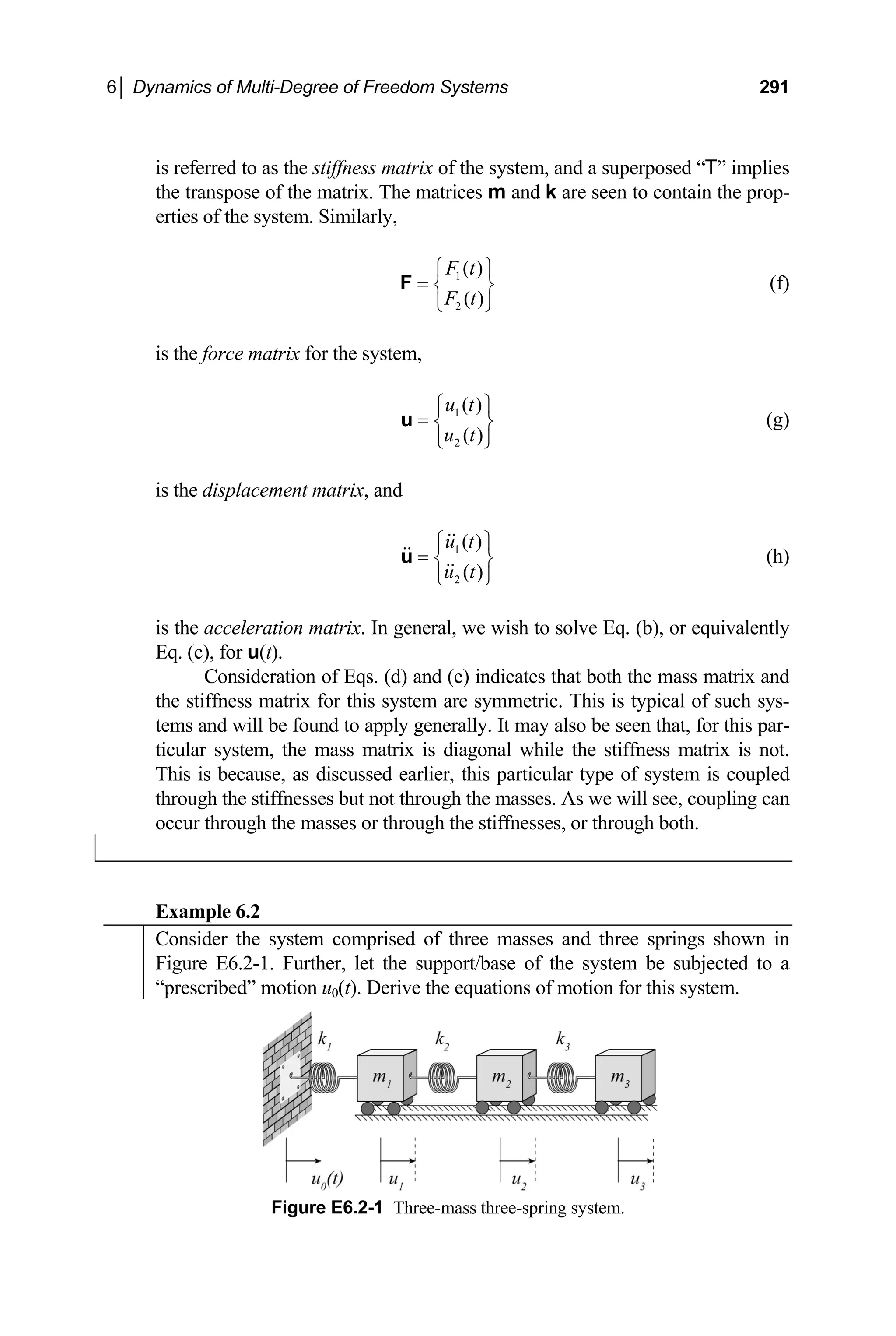
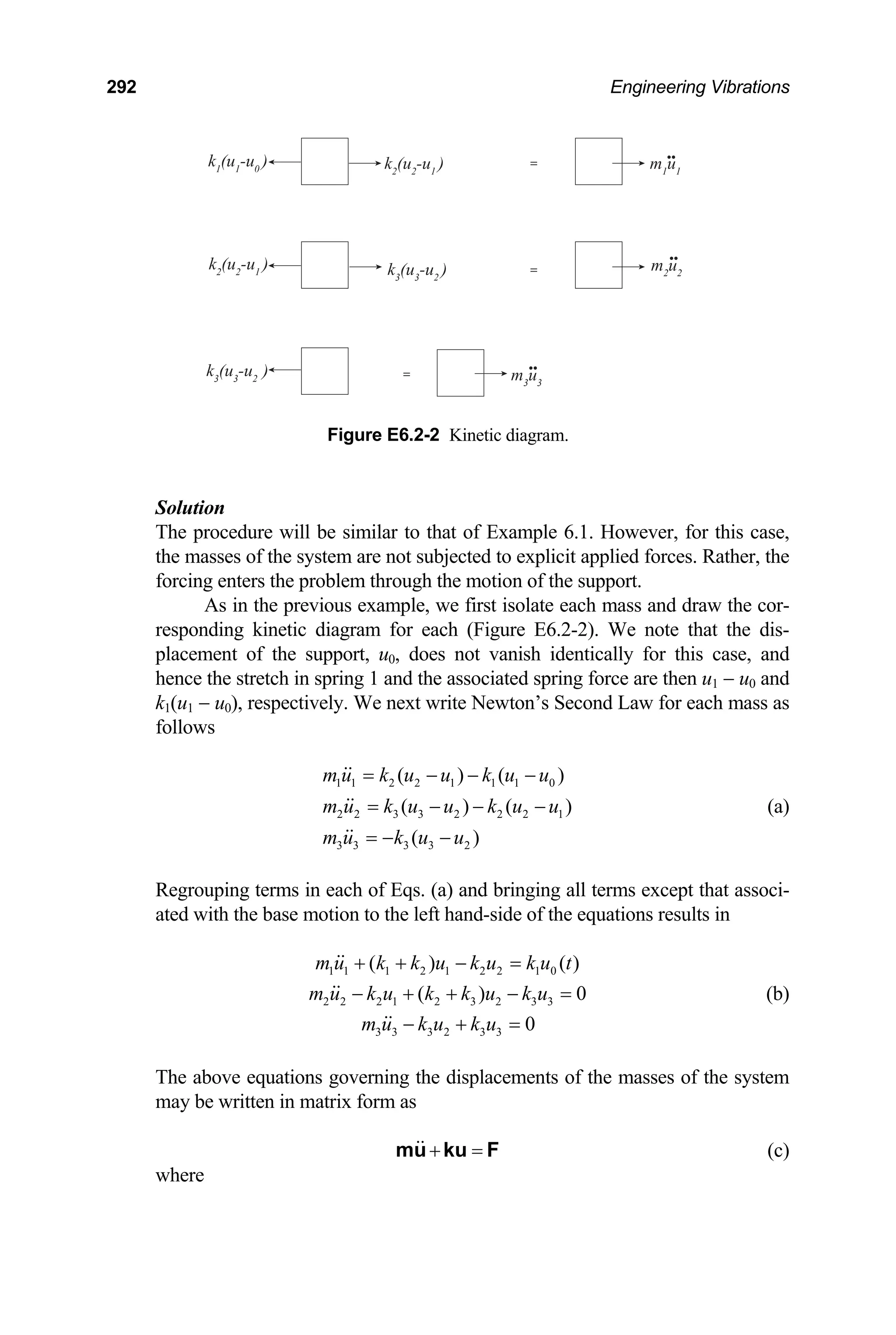
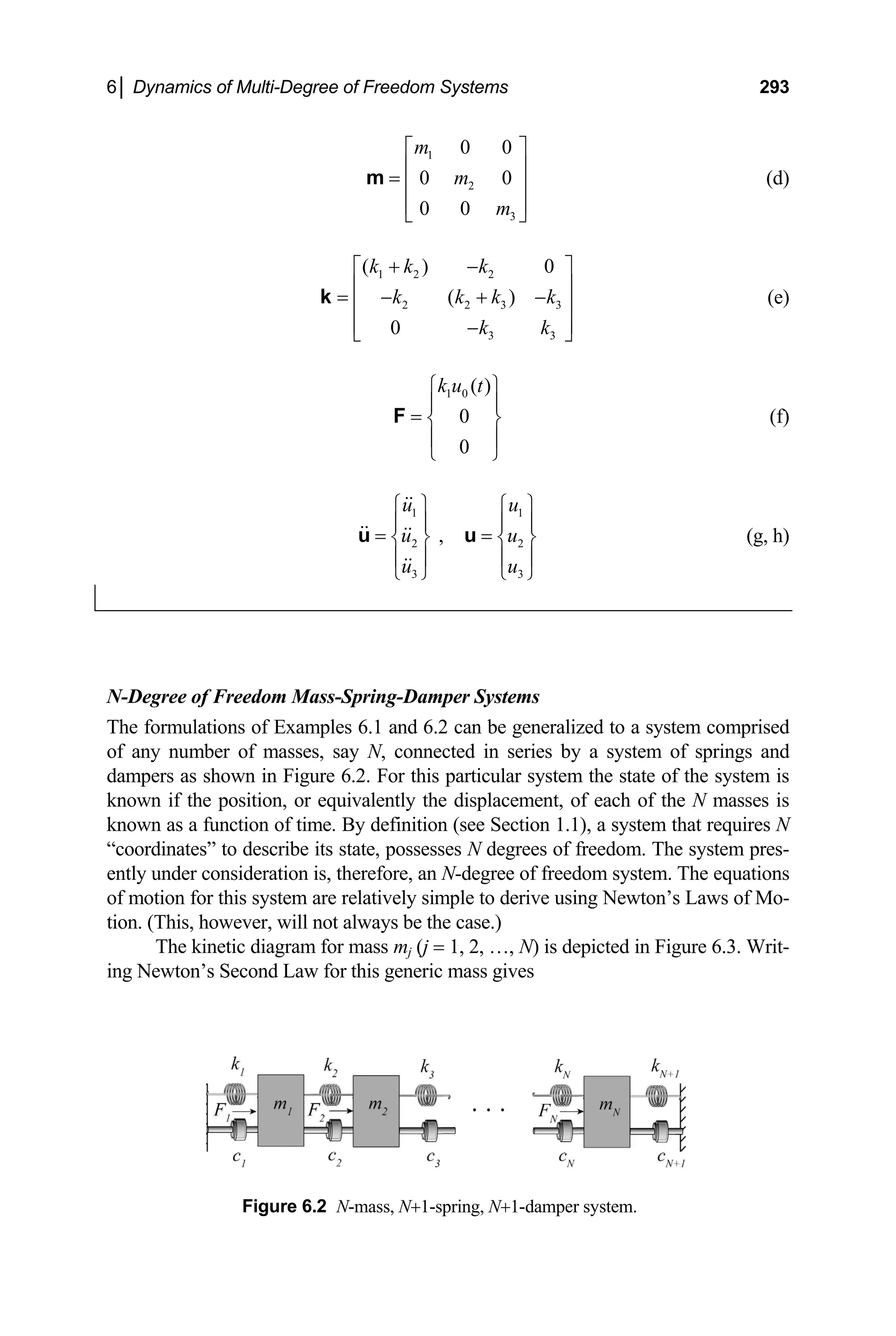
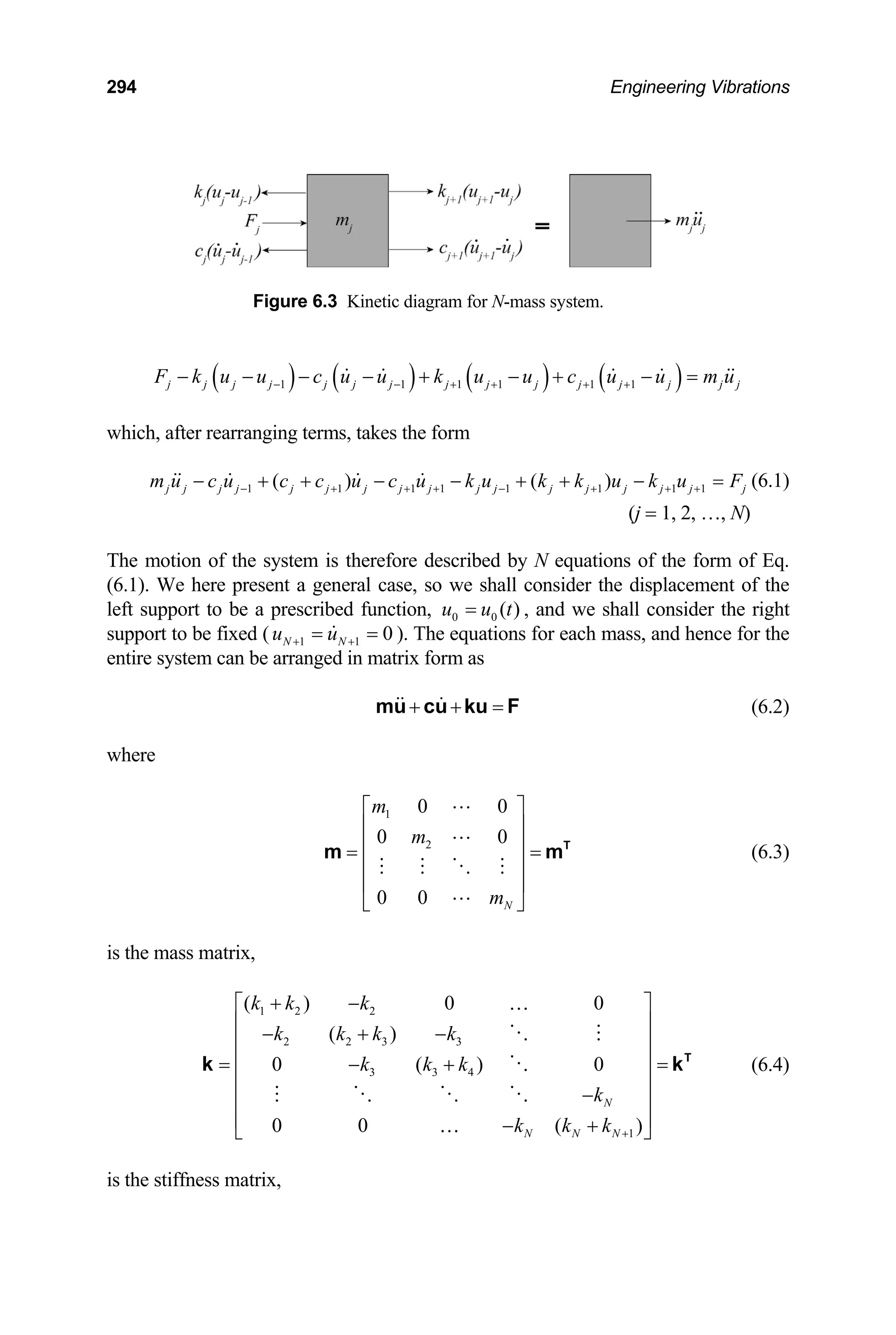
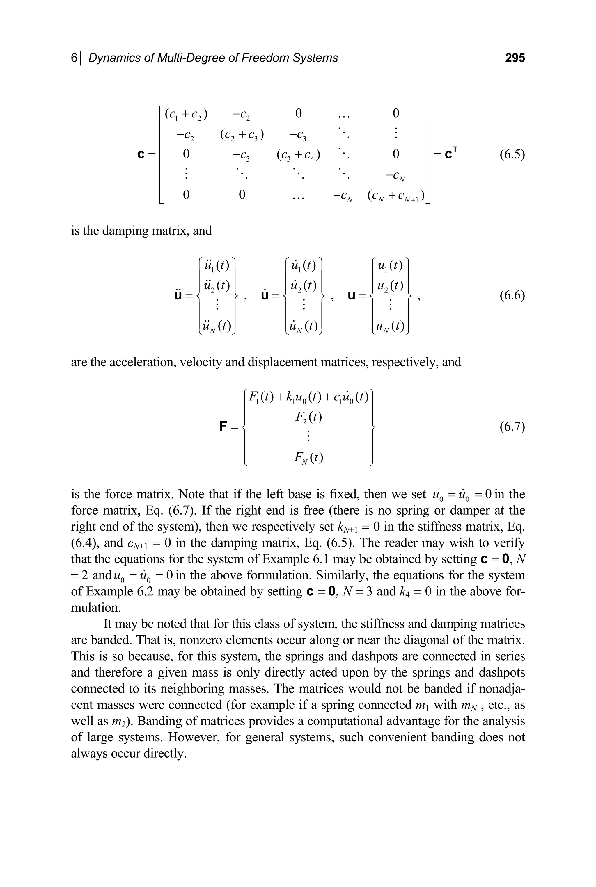
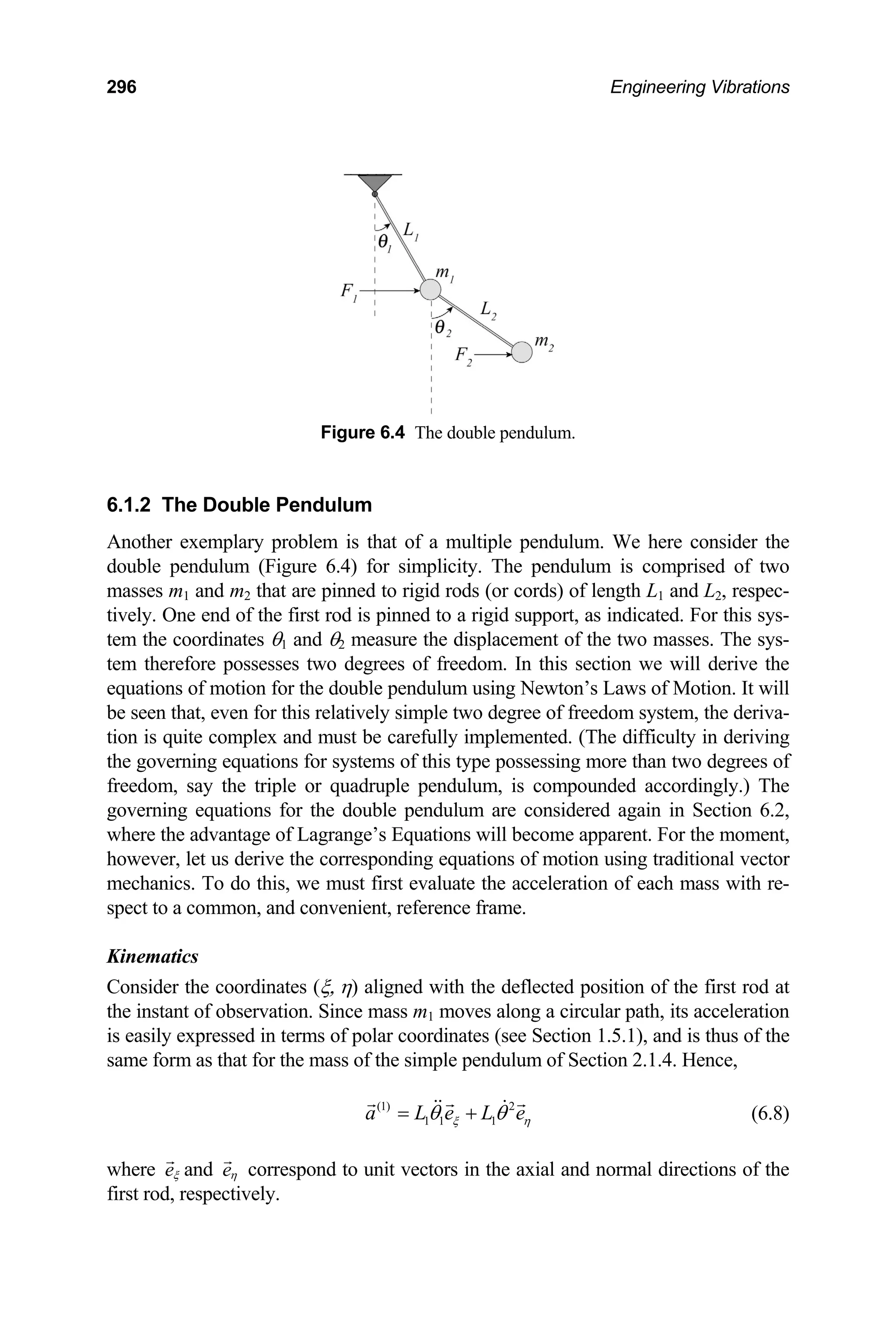
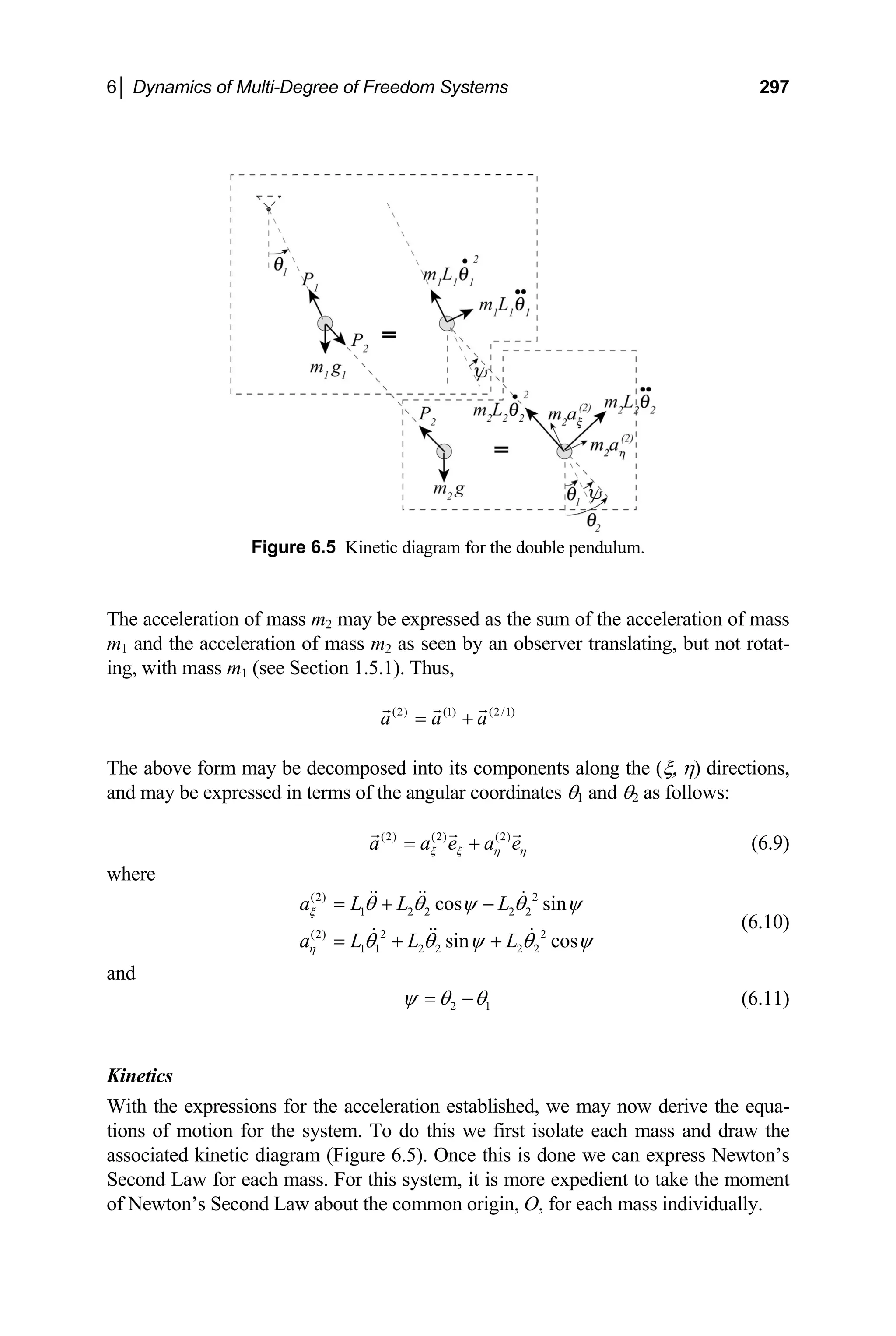
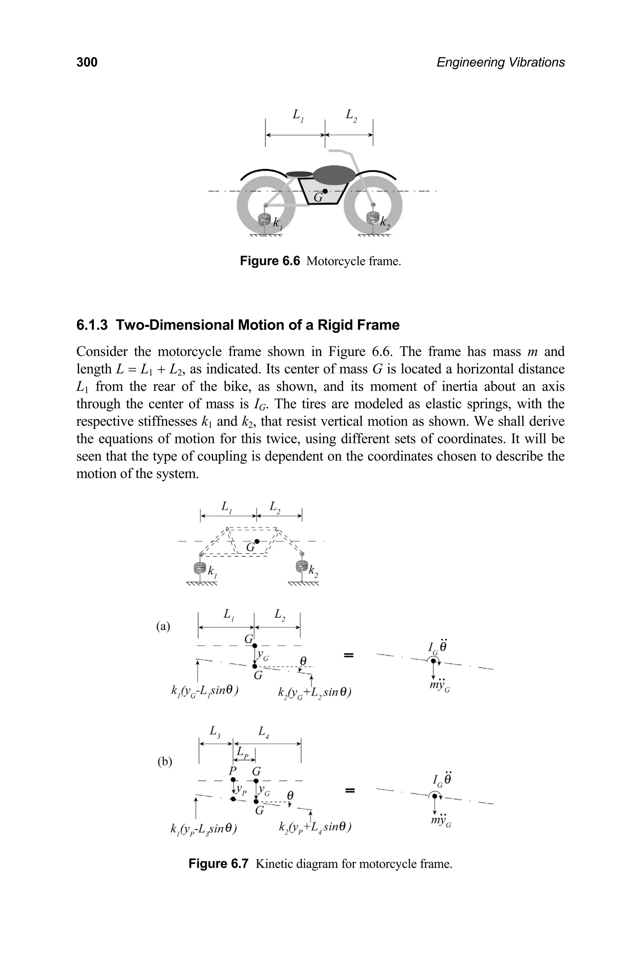
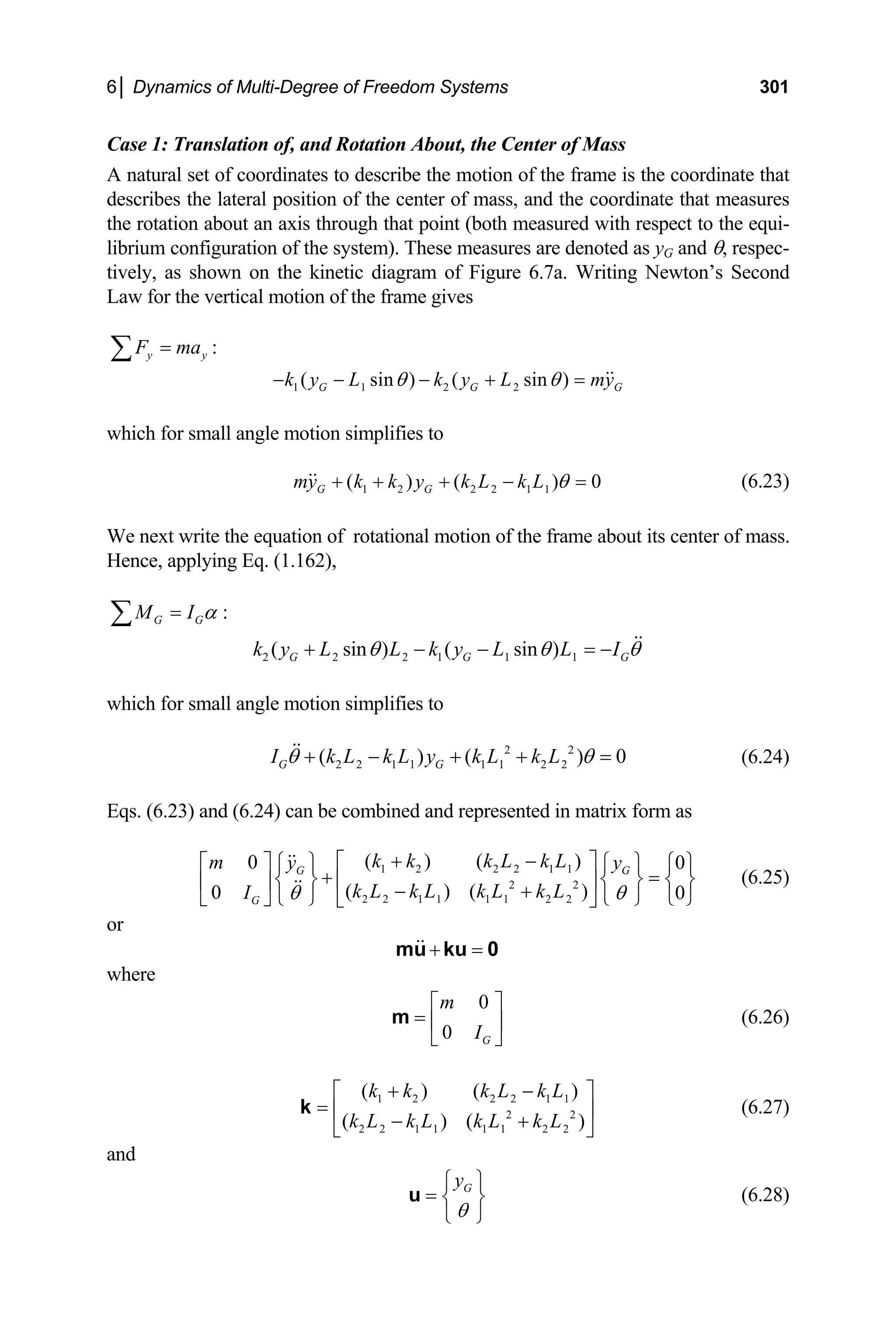
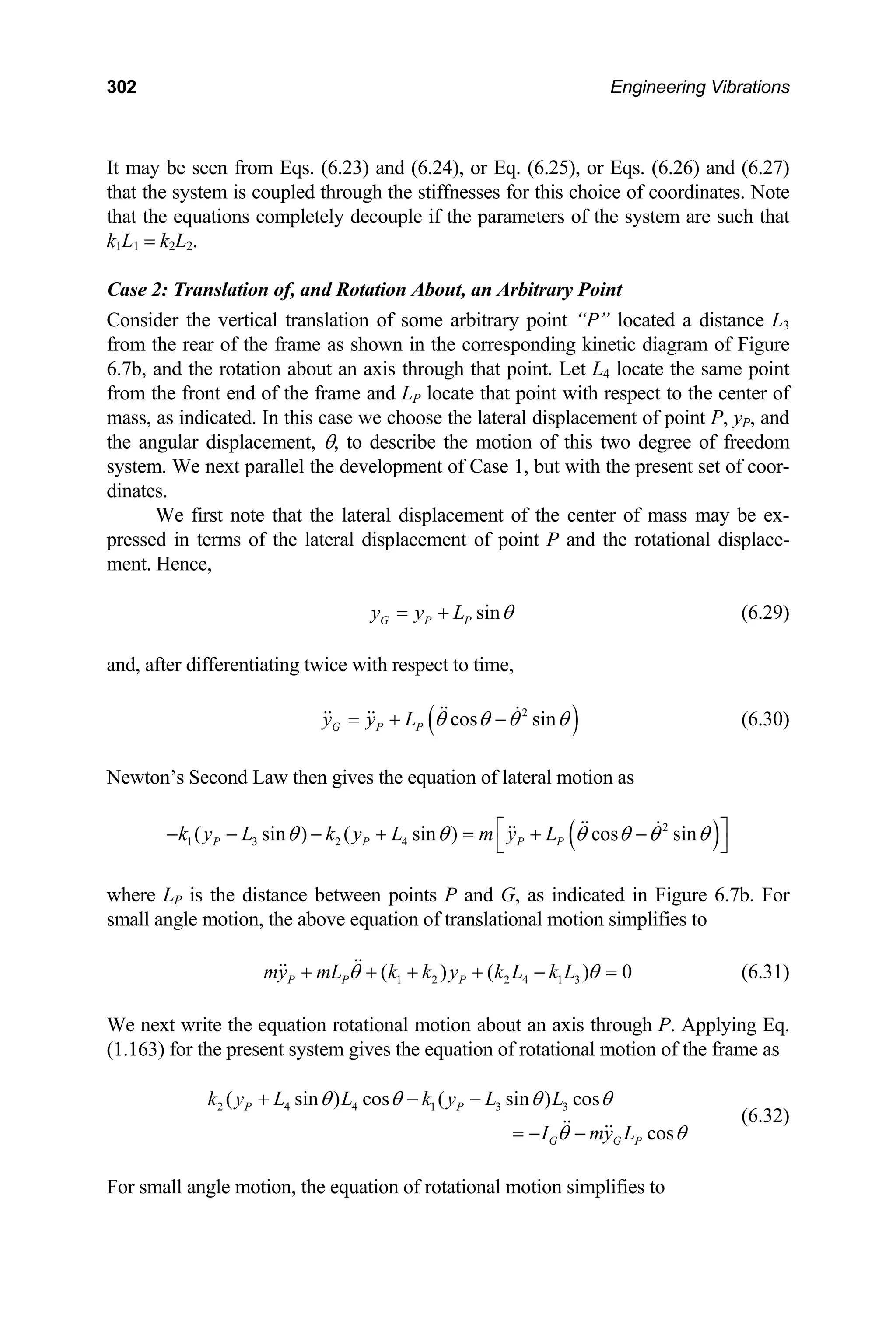
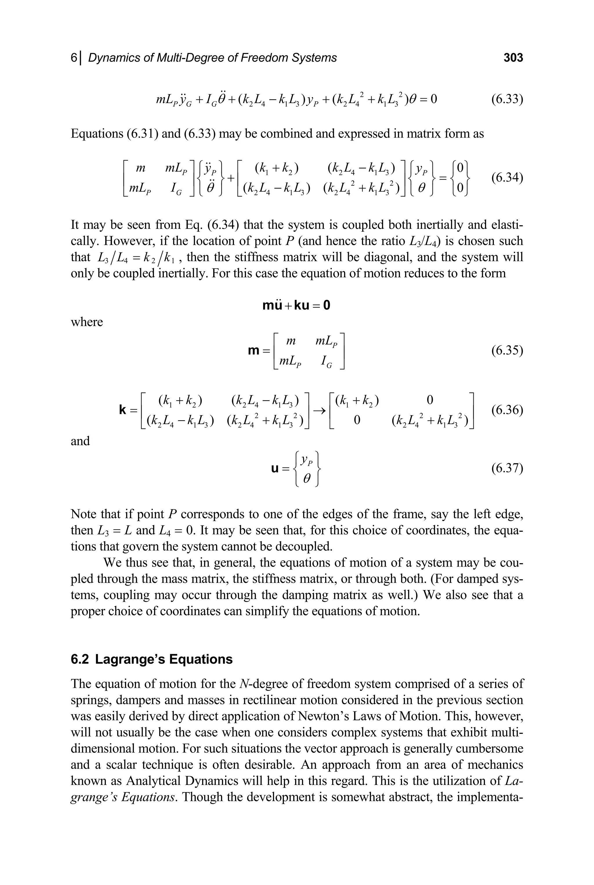
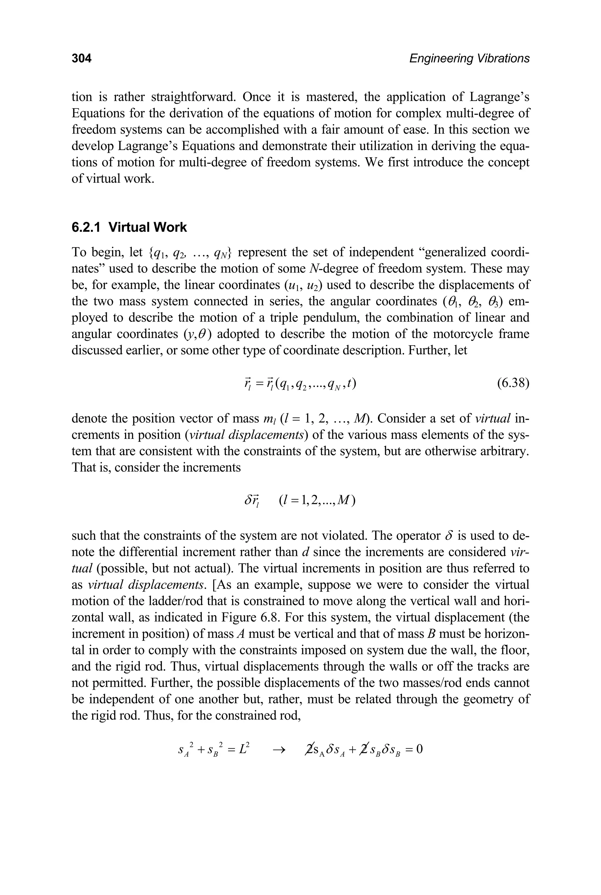
![6│ Dynamics of Multi-Degree of Freedom Systems 305
sA
A
L
B
sB
Figu tem.
here sA and sB respectively locate the positions of mass A and mass B, as indicated.]
em, the virtual work
one by the external force and by the resultant internal force acting on mass ml , as the
ass moves through the corresponding virtual displacement
re 6.8 Example of a constrained sys
w
Returning to the discussion of a general N-degree of freedom syst
d
m l
r
δ , is then
( )
( ) ( )
ext int
l l l l
F F r
δ δ
= + i
W
int
l lj
j
F
=
=
(6.39)
where,
M
( )
1
∑P (6.40)
e internal force exerted on mass ml by mass mj, and it is understood that
= =
P P P (i.e., no mass exerts a force on itself). It follows from New-
n’s Third Law that
lj
P is th
= =
11 22 ... 0
MM
jl l
= −
P P (
to j l, j = 1, 2, …, M),
1
int
l
j
F
=
=
∑ ∑∑
he work done by the forces acting on each particle of the system as
xpressed by Eq. (6.39), and noting that the internal forces of the system sum to
as expressed by Eq. (6.41), gives the total virtual work done on the system as
and hence that
( )
11 12 1 1 2
1 1
( ... ) ... ( ... ) 0
M M M
lj M M M MM
l l
= =
= + + + + + + + + =
P P P P P P P (6.41)
Thus, adding t
e zero
1 1
M M
l l l
l l
F r
δ δ δ
= =
= =
∑ ∑ i
W W (6.42)
where l
F includes external forces, and those internal forces for which the associated
isplacement can differ from that of the force’s mirror im
d age.](https://image.slidesharecdn.com/engineeringvibrations-240713005818-b85f16c0/75/Engineering-Vibrations-Engineering-Vibrations-327-2048.jpg)
![6│ Dynamics of Multi-Degree of Freedom Systems 311
j = 1:
( ) [ ]
1 1 1 1 1 2 2 1 1
1 1
( )
Q m u k u k u u F
dt q q dt
d d
⎛ ⎞
∂ ∂
− = → − − + − =
⎜ ⎟
∂ ∂
egrouping terms results in the equation of motion for the first mass,
⎝ ⎠
L L
R
1 1 1 2 1 2 2 1
( )
m u k k u k u F
+ + − = (e)
j = 2:
( )
2 2 2 2 2 1 3 3 2 2
( ) ( )( 1)
d d
Q m u k u u k u u F
⎛ ⎞
∂ ∂
− = → + − + − − =
⎜ ⎟
2 2
dt q q dt
∂ ∂
L L
This results in the equation of motion for the secon
⎝ ⎠
d mass,
2 2 2 1 2 3 2 3 3 2
( )
m u k u k k u k u F
− + + − = (f)
3:
j =
( ) [ ]
3 3 3 3 3 2 3
( )
d d
Q m u k u u F
⎛ ⎞
∂ ∂
− = → − − − =
⎜ ⎟
3 3
dt q q dt
∂ ∂
L L
which gives the equation of motion for the third mass,
⎝ ⎠
3 3 3 2 3 3 3
m u k u k u F
− + = (g)
qs. (e)–(f) may be combined in matrix form as
2 2 2 2 3 3 2 2
3 3 3
0 0 0
u F
u F
m u k
E
1 1 1 2 2
0 0 ( ) 0
0 0 ( )
m u k k k
m u k k k k
+ − 1 1
3 3 3
k u F
⎪ ⎪ ⎪ ⎪
⎥
⎦ ⎩ ⎭ ⎩ ⎭
⎡ ⎤ ⎧ ⎫ ⎧ ⎫
⎪ ⎪ ⎪ ⎪
=
⎨ ⎬ ⎨ ⎬
⎢ ⎥ ⎢ ⎥
⎪ ⎪
⎢ ⎥ ⎢ −
⎣ ⎦ ⎩ ⎭ ⎣
(h)
(6.2)–(6.6) for the case where
= 3, k4 = 0 and c = 0.
⎧ ⎫ ⎡ ⎤
⎪ ⎪
⎢ ⎥ ⎢ ⎥
+ − + −
⎨ ⎬
Equation (h) may be compared directly with Eqs.
N 0 0
u ≡ ,
Example 6.4
Use Lagrange’s Equations to derive the equations of motion for the 3-mass 3-
spring 3-damper system of Figure E6.4-1.](https://image.slidesharecdn.com/engineeringvibrations-240713005818-b85f16c0/75/Engineering-Vibrations-Engineering-Vibrations-333-2048.jpg)
![312 Engineering Vibrations
Solution
To derive the equations of m st add the virtual work
of the viscous dam rtual work of the applied forces when
evaluating the total vir the nonconservative forces that act on
. We may then proceed as we did for the undamped 3 mass system of
, with the c diagram depicted in Figure E6.4-
ual work done by the nonconservative forces is given by
Figure E6.4-1
otion for this system we mu
ping forces to the vi
tual work done by
the system
Example 6.3. Thus aid of the kineti
2, the virt
[ ] [ ]
[ ]
( )
1 1 2 2 3 3
1 1 1 2 2 1 1 2 2 2 1 3 3 2 2
3 3 3 2 3
( ) ( ) ( )
( )
NC
Q u Q u Q u
F c u c u u u F c u u c u u u
F c u u u
δ δ δ δ
δ δ
δ
= + +
= − + − + − − + −
+ − −
W
(a)
he generalized forces are then given by the coefficients of the
T
p
virtual dis-
lacements in Eq. (a). Hence,
2
1 1 1 2 1 2
( )
Q F c c u c u
= − + + (b)
3
2 2 2 1 2 3 2 3
( )
Q F c u c c u c u
= + − + + (c)
3
3 3 3 2 3
Q F c u c u
= + − (d)
gies for the damped system are the same as for
e undamped system of the previous example. Therefore, incorporating the
damping forces into the generalized forces in the
ample 6.3 modifies the right hand side of the resultin
example to the form
Figure E6.4-2 Kinetic diagram.
The potential and kinetic ener
th
development put forth in Ex-
g matrix equation of that](https://image.slidesharecdn.com/engineeringvibrations-240713005818-b85f16c0/75/Engineering-Vibrations-Engineering-Vibrations-334-2048.jpg)
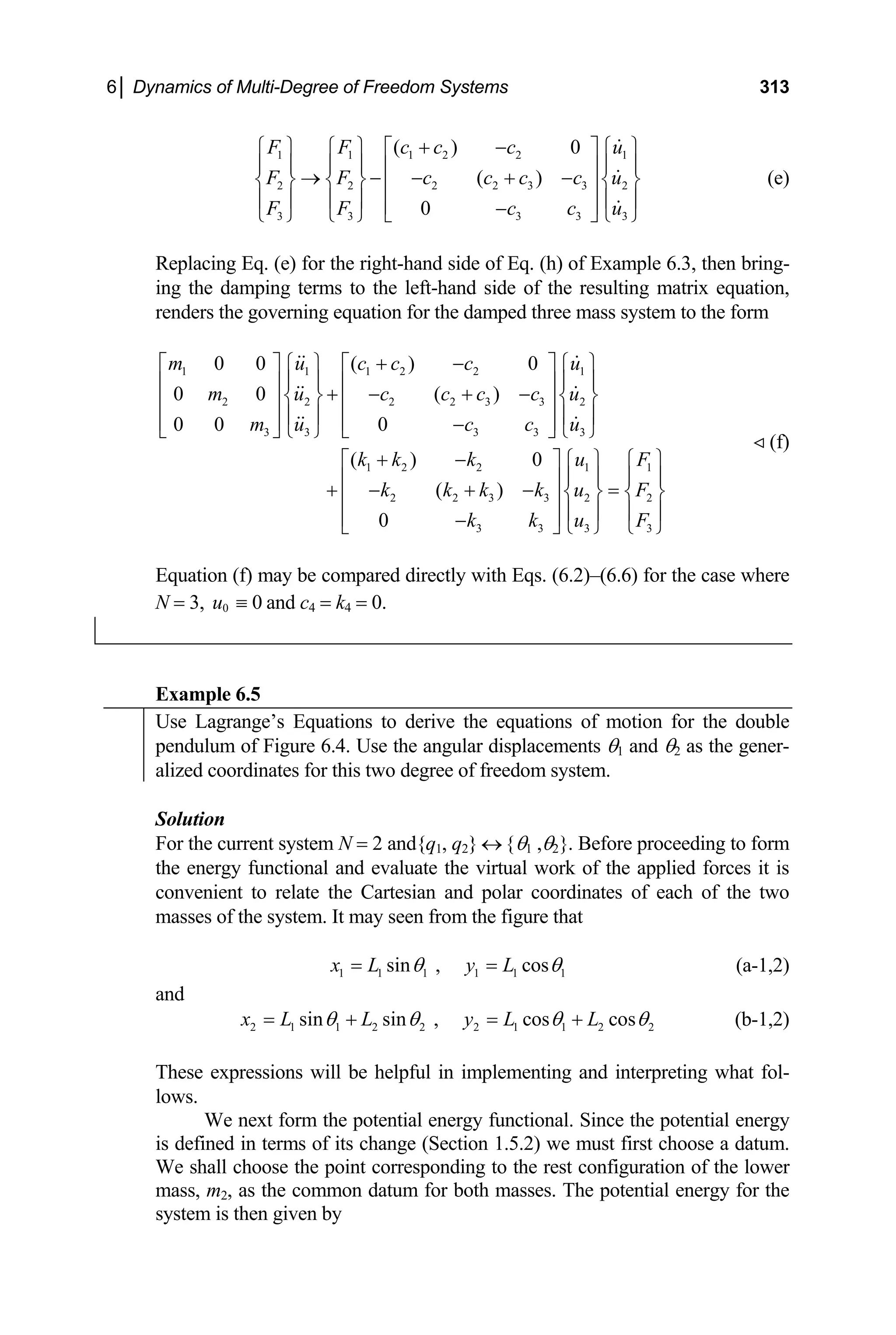
![314 Engineering Vibrations
)
1 1 2 2 1 1 2 1 2 1 2 2
( ) (
m gh m gh m g L L y m g L L y
= + = + − + + −
U (c)
Substituting the coordinate transformation described by Eqs. (a) and (b) into
Eq. (c) gives the potential energy in terms of the angular coordinates θ1 and θ2
as
[ ] [ ]
1 1 1 2 2 1 1 2 2 )
(1 cos ) (1 cos ) (1 cos
m g L L m g L L
θ θ θ
= − + + − + −
U (d)
The kinetic energy of the system is easily written as
( ) ( )
2 2 2 2 2 2
1 1 1 1
m v m v m x y m x y
= + = + + +
T (e)
1 1 2 2 1 1 1 2 2 2
2 2 2 2
Substituting Eqs. (a) and (b) into Eq. (e) gives
( ) ( )
( ) (
2 2
2 1 1 1 2 2 2 1 1 1 2 2
2
1
cos cos sin sin
2
m L L L L
θ θ θ θ θ θ θ
⎣ ⎦
⎡ ⎤
+ + + − −
⎢ ⎥
⎣ ⎦
(f)
2 2
1 1 1 1 1 1 1
1
cos sin
m L L
θ θ θ θ
⎡ ⎤
= + −
⎢ ⎥
T
)
2
θ
hich, when expanded, takes the simple form
w
2 2 2 2
1 1
1 2 1 1 2 2 2 2 1 2 1 2 1 2
2 2
( ) cos(
m m L m L m L L )
θ θ θ θ θ
= + + + −
T θ (g)
It is instructive to note that Eq. (f) could be obtained directly by calculating the
lative velocity of m2 with respect to m1 and adding it to the velocity of the
in Figure 6.5 and discussed in
f each mass in terms of its com-
ponents with respect to the path coordinates of the first mass at a given instant
in time, we have
re
first mass using the reference frame depicted
Section 6.1.2. Hence, expressing the velocity o
1 1 1
v L eξ
θ
= (h)
2 1 2/1 1 1 2 2 2 1 2 1
cos( ) sin( )
v v v L e L e e
ξ ξ η
θ θ θ θ θ θ
⎡ ⎤
= + = + − + −
⎣ ⎦ (i)
It follows directly that
2
v v v L
2 2
1 1 1 1 1
θ
= =
i (j)
and
2 2
2 2 2 2 2
2 2 2 1 1 1 2 1 2 2 1 2 2
2 cos( )
v v v L L L L
θ θ θ θ θ θ
= = + − +
i (k)](https://image.slidesharecdn.com/engineeringvibrations-240713005818-b85f16c0/75/Engineering-Vibrations-Engineering-Vibrations-336-2048.jpg)
![6│ Dynamics of Multi-Degree of Freedom Systems 315
Substitution of Eqs. (j) and (k) into Eq. (e) then gives the kinetic energy in the
form of Eq. (f).
The last things we must determine before we
are the generalized forces Q1 and Q2. To do this we must evalua
tual work of the applied forces F1 and F2. Since the indicated
the horizontal, the virtual work of these forces is simply
NC
F x F x
tions
can apply Lagrange’s Equa-
te the vir-
forces act along
( )
1 1 2 2
δ δ δ
= + (l)
1
W
However, we must express everything in terms of the chosen generalized coor-
dinates, θ1 and θ2. Now, it follows from Eqs. (a) and (b) that
1 1 1
cos
x L
δ θ δθ
=
nd
(m-1)
a
2 1 1 1 2 2 2
cos cos
x L L
δ θ δθ θ δθ
= + (m-2)
ubstitu -1) and (m-2) into Eq. (l) gives the virtual work of the
S
applied forces
tion of Eqs. (m
in the desired form. Hence,
( )
( )
1 1 2 2 1 2 1 1 1
cos
NC
Q Q F F L 2 2 2 2
cos
F L θ δθ (n)
δ δθ δθ θ δθ
= + = + +
W
1 2
From Eq. (6.58), the generalized forces associated with the chosen coordinates
are the coefficients of the virtual displacements δθ and δθ . These may be read
irectly from Eq. (n) to give
d
( )
1 1 2 1 cos
Q F F L 1
θ
= + (o-1)
2 2 2 2
cos
Q F L θ
= (o-2)
[N
cation of Eq. (
ote that the generalized forces may have also been computed by direct appli-
6.59).] It may be seen that, for t
actually moments. This is, of course, as it should be since the vir
lacements are angular. Equations (d), (g) and (o) m
rectly into Eqs. (6.62) and (6.63). Carrying
ith {q , q θ ,θ }, gives the equations of motion for the double pendu-
his case, the generalized forces
tual dis-
are
p ay now be substituted di-
through the required calculations,
w 1 2} ↔ { 1 2
lum. Hence,
j = 1:
1
1 1
d
Q
dt q q
⎛ ⎞
∂ ∂
− = ⇒
⎜ ⎟
∂ ∂
⎝ ⎠
L L](https://image.slidesharecdn.com/engineeringvibrations-240713005818-b85f16c0/75/Engineering-Vibrations-Engineering-Vibrations-337-2048.jpg)
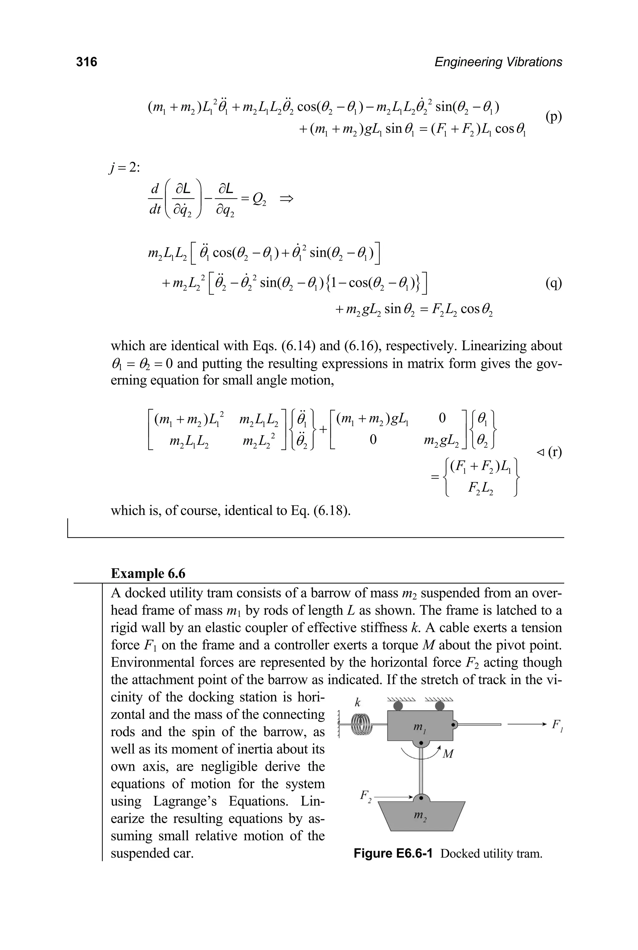
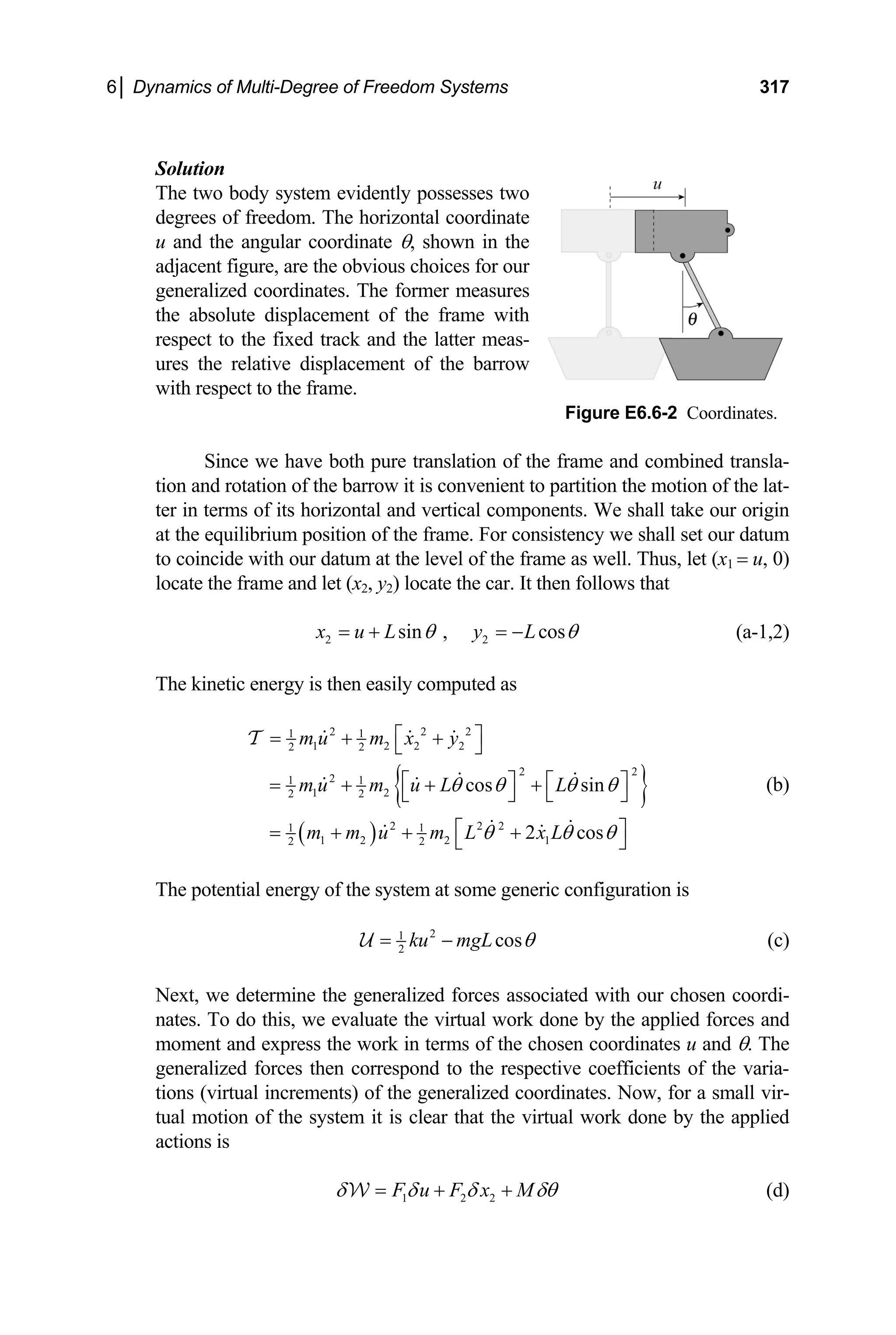
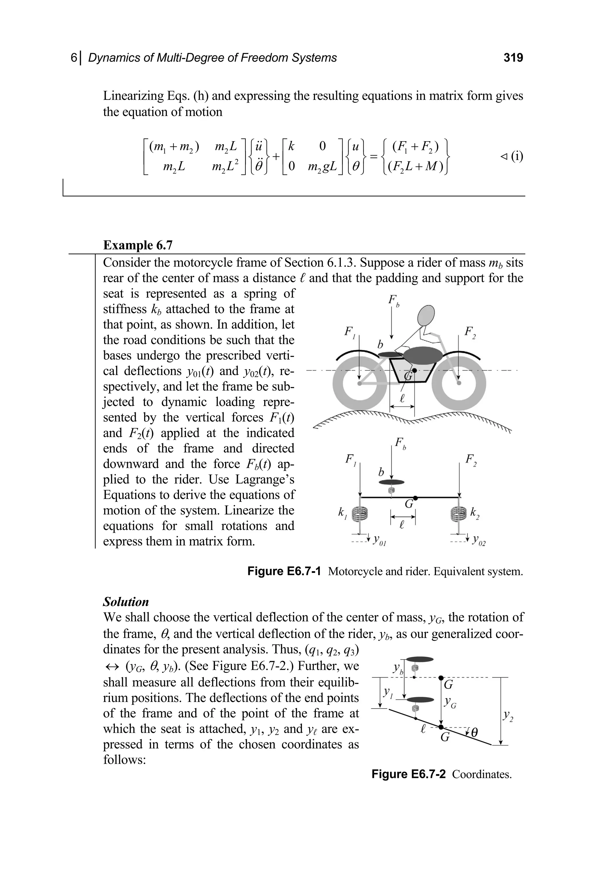
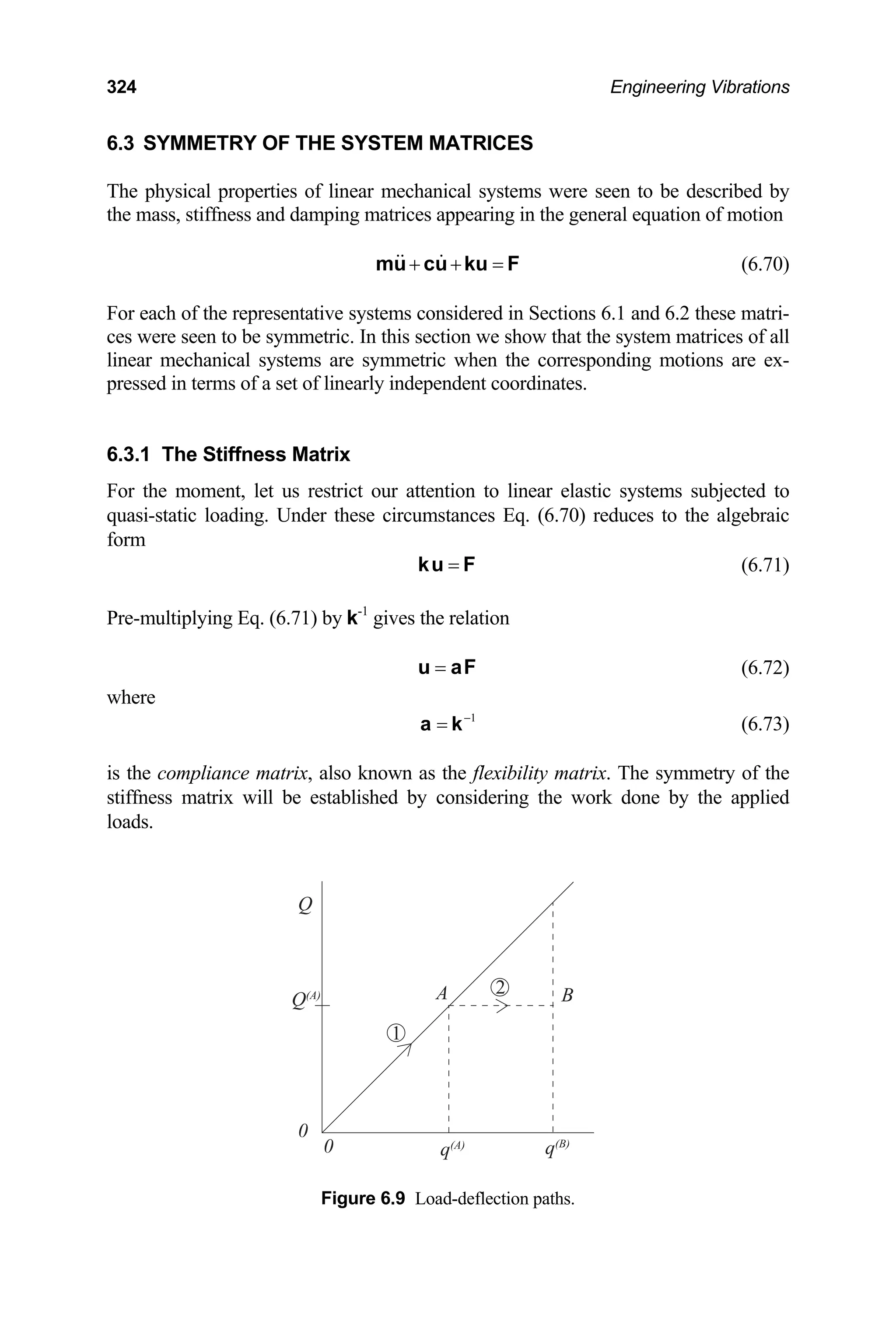
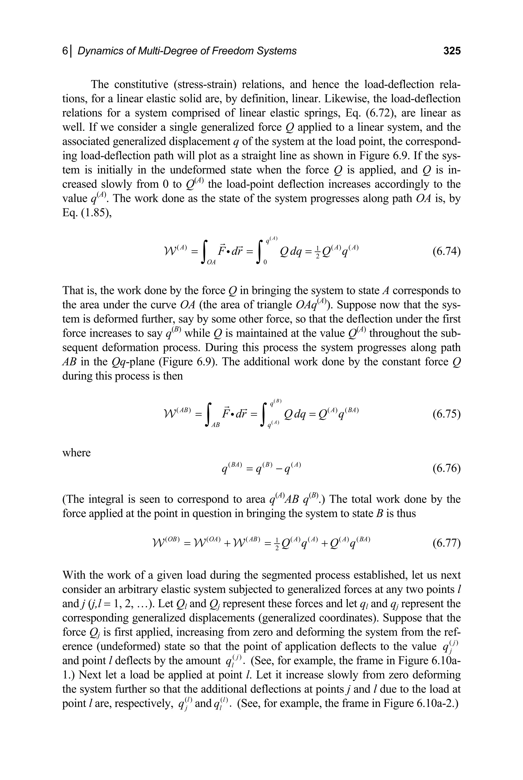
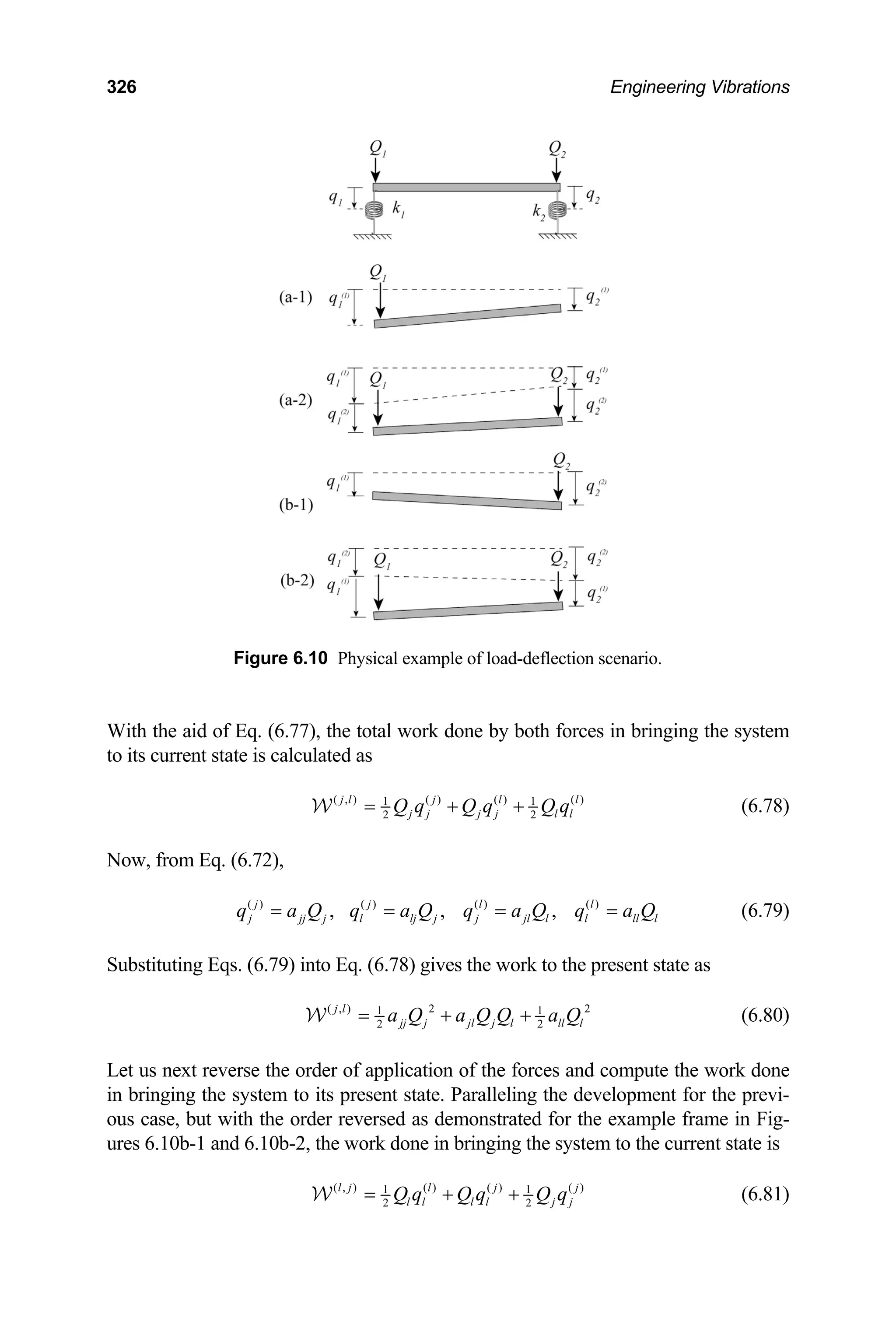
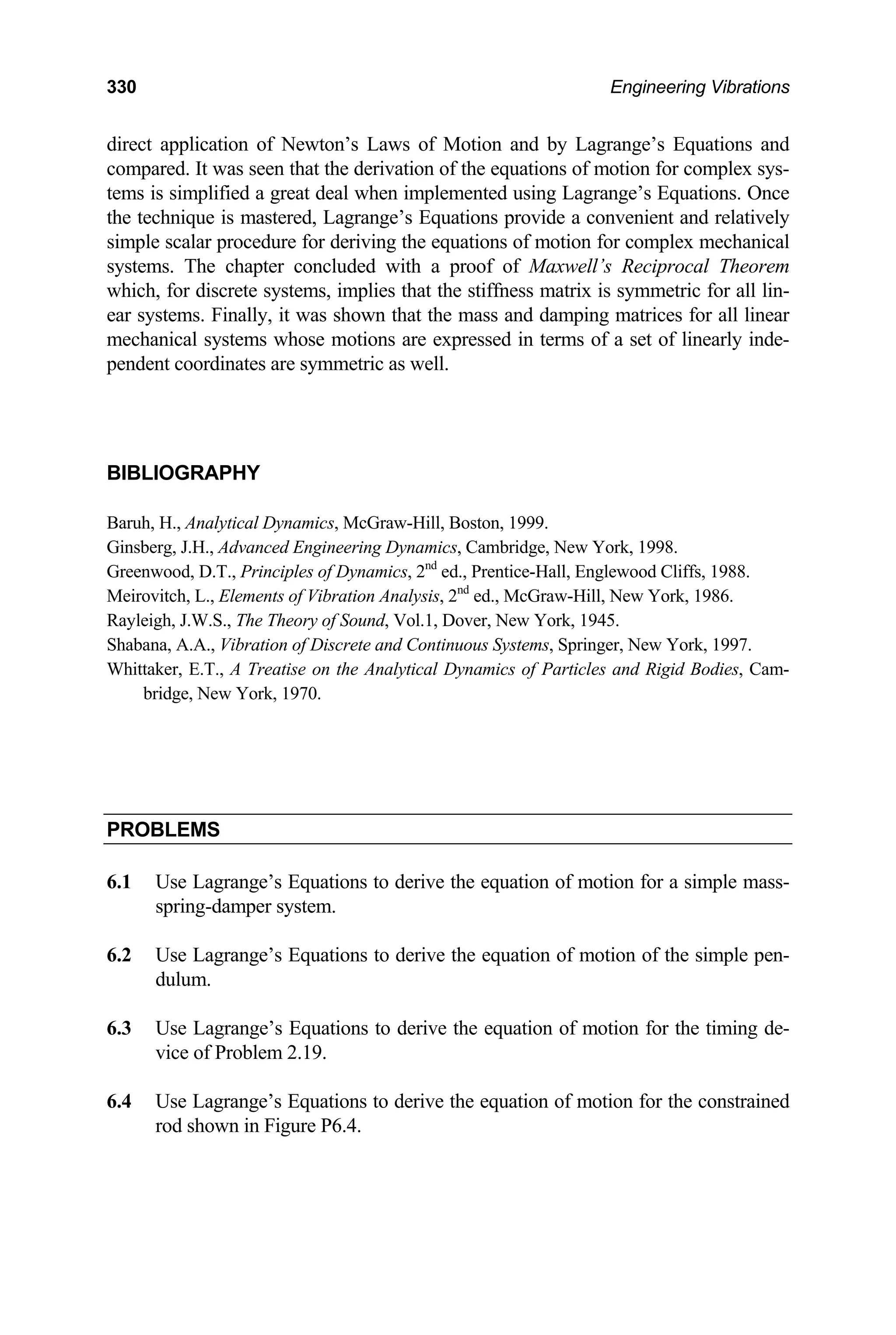
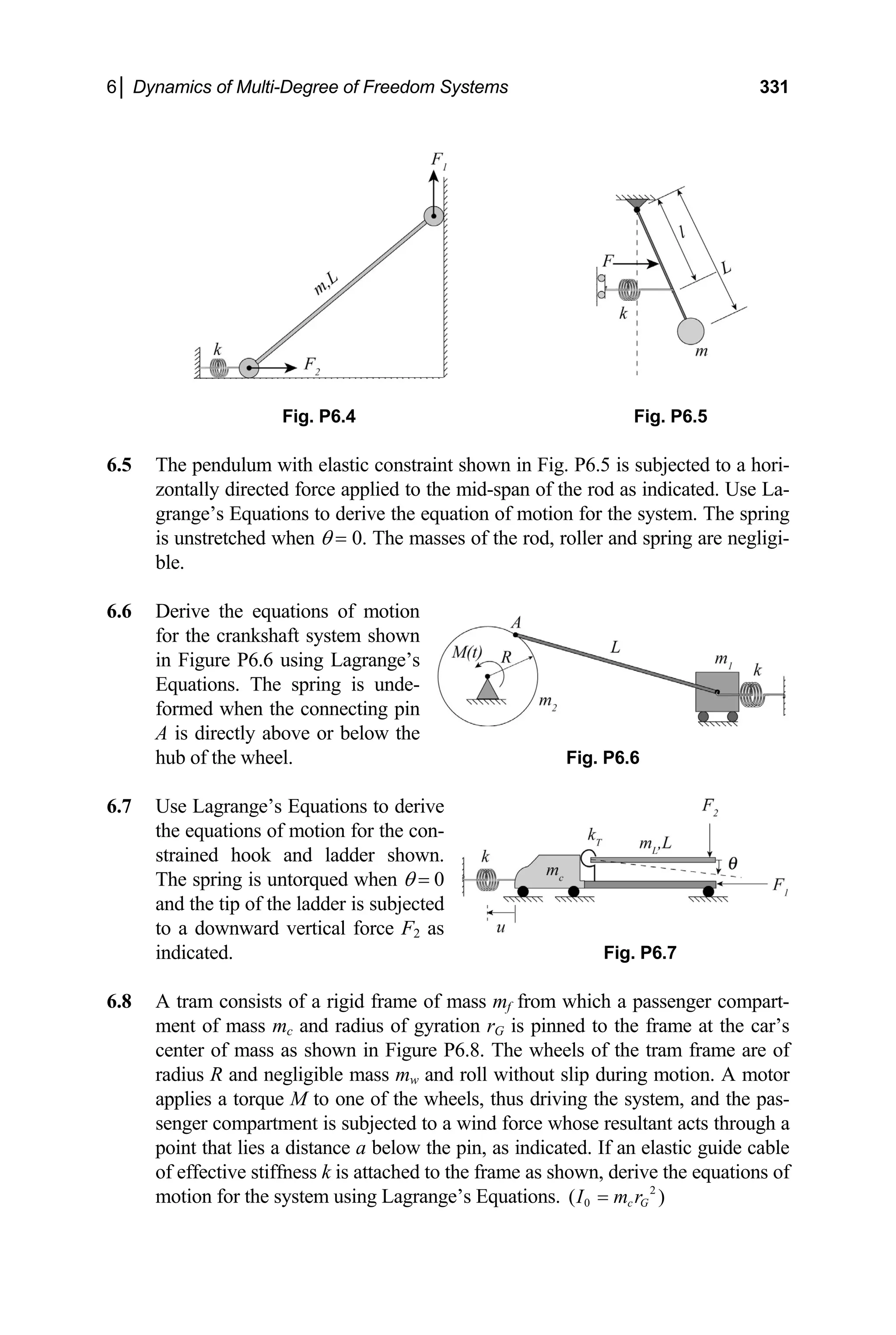

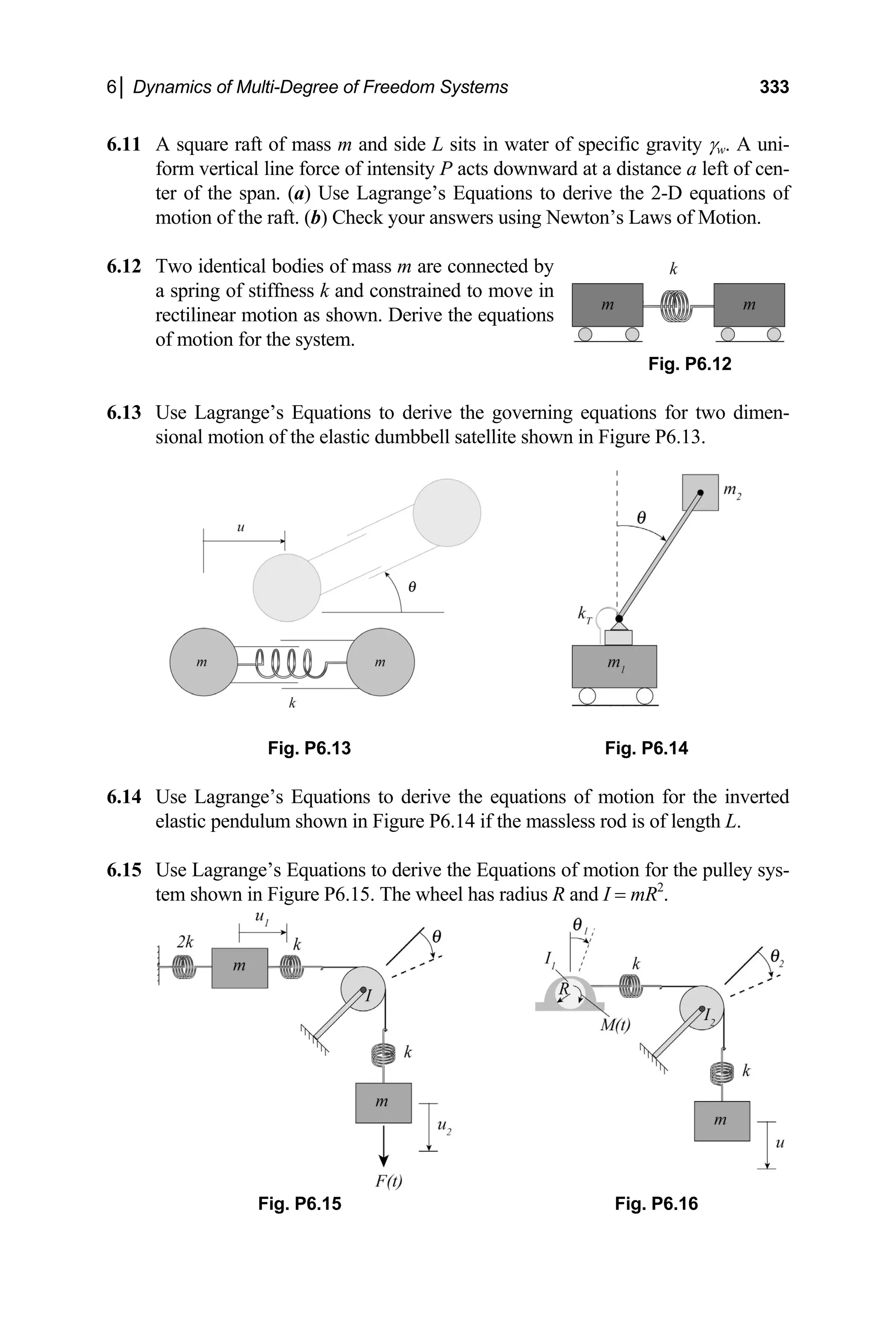
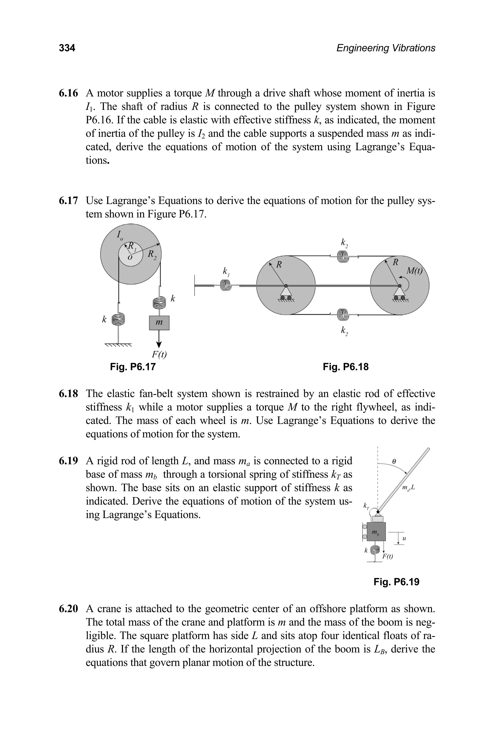
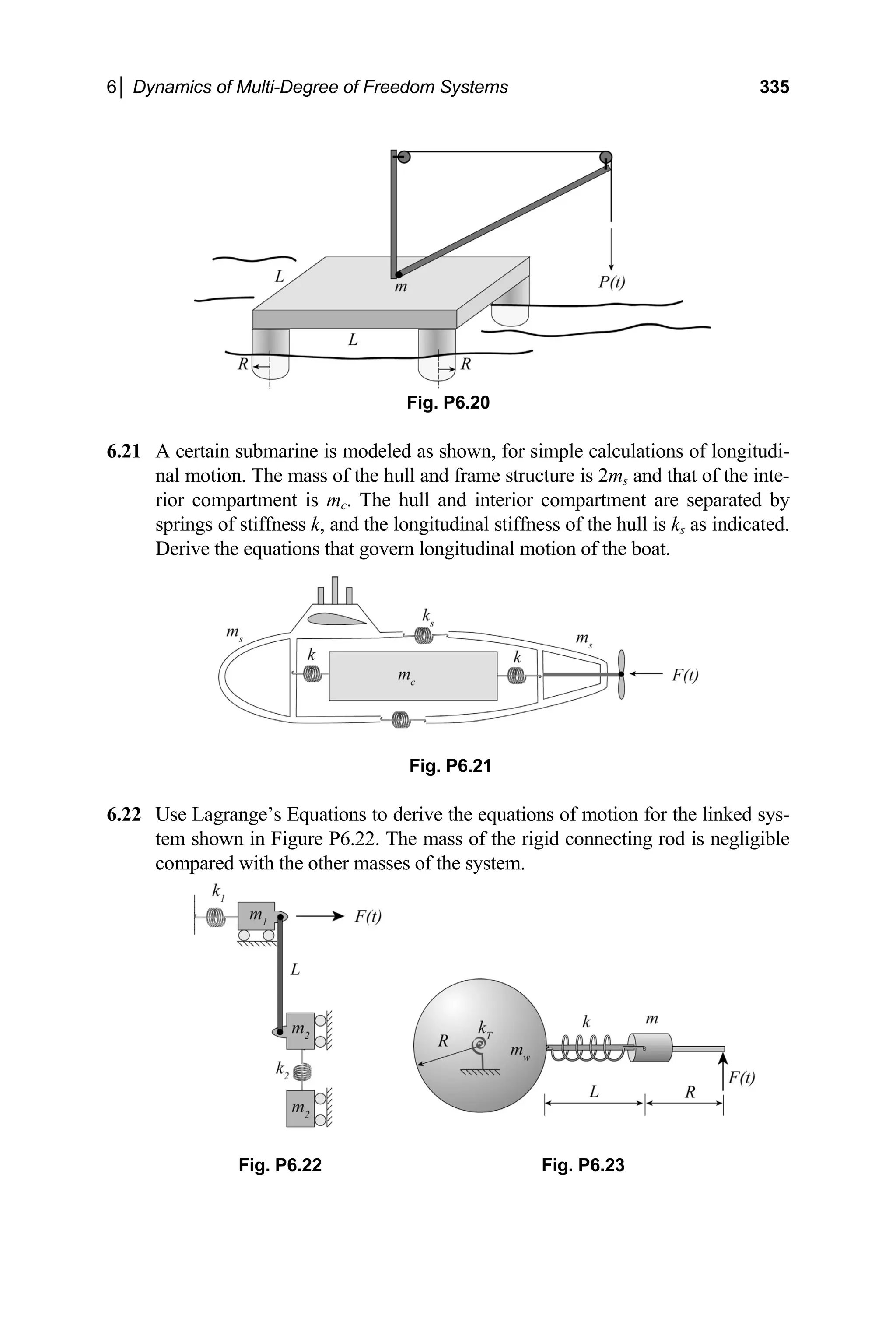
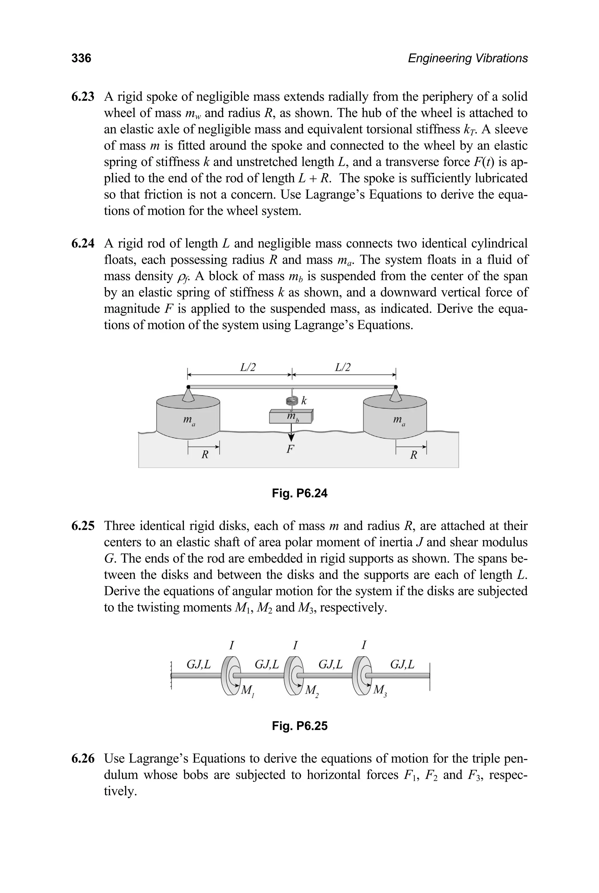
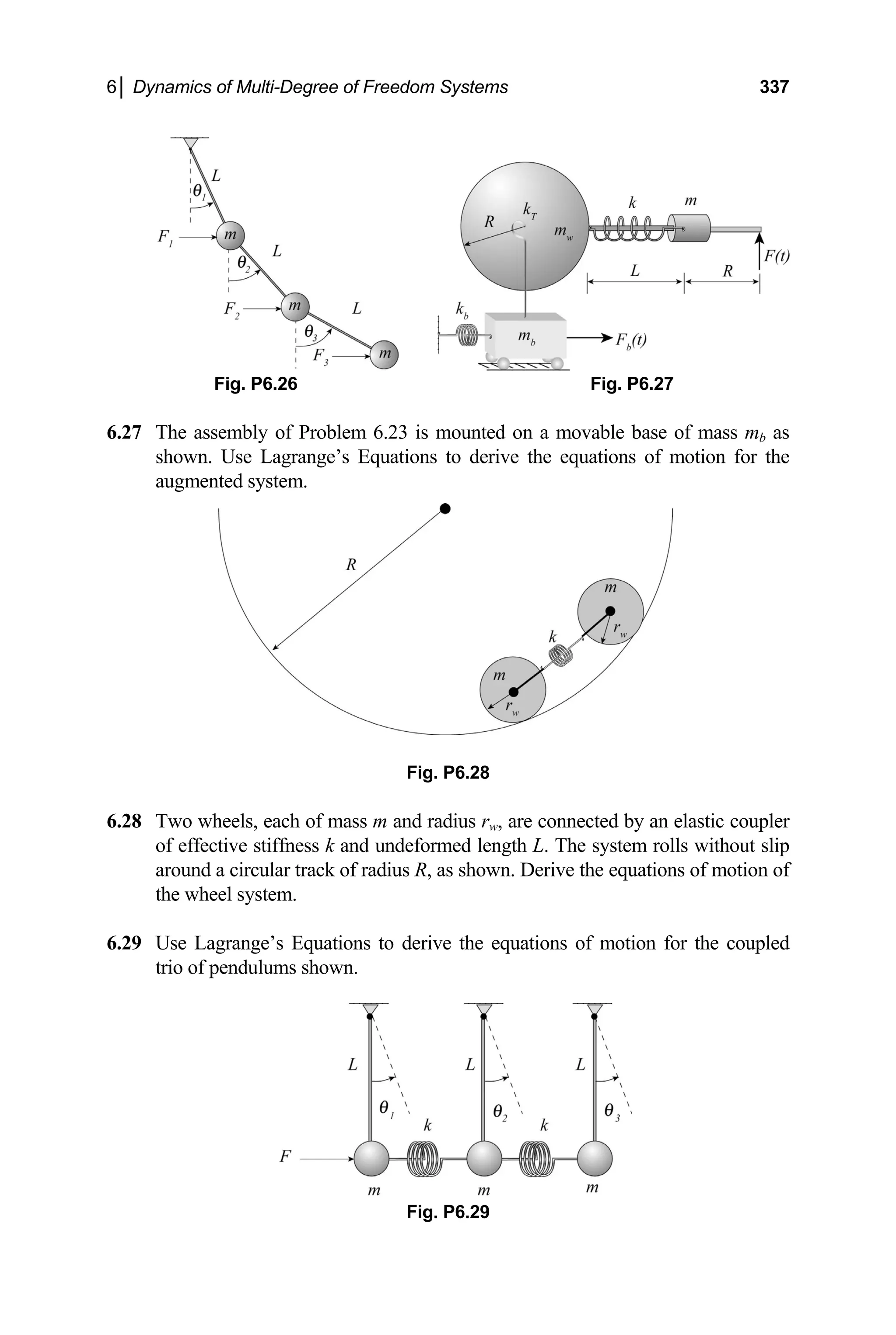
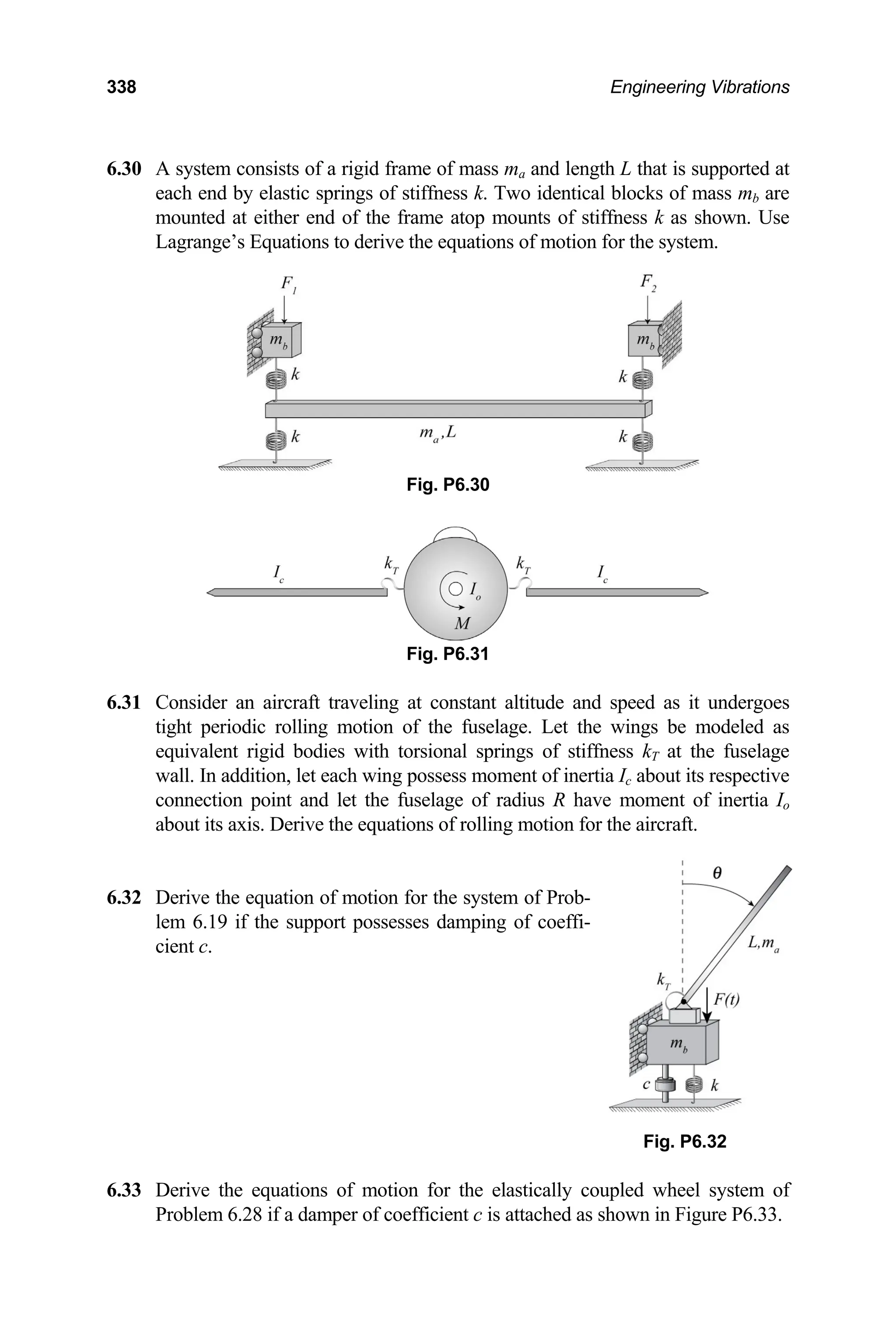
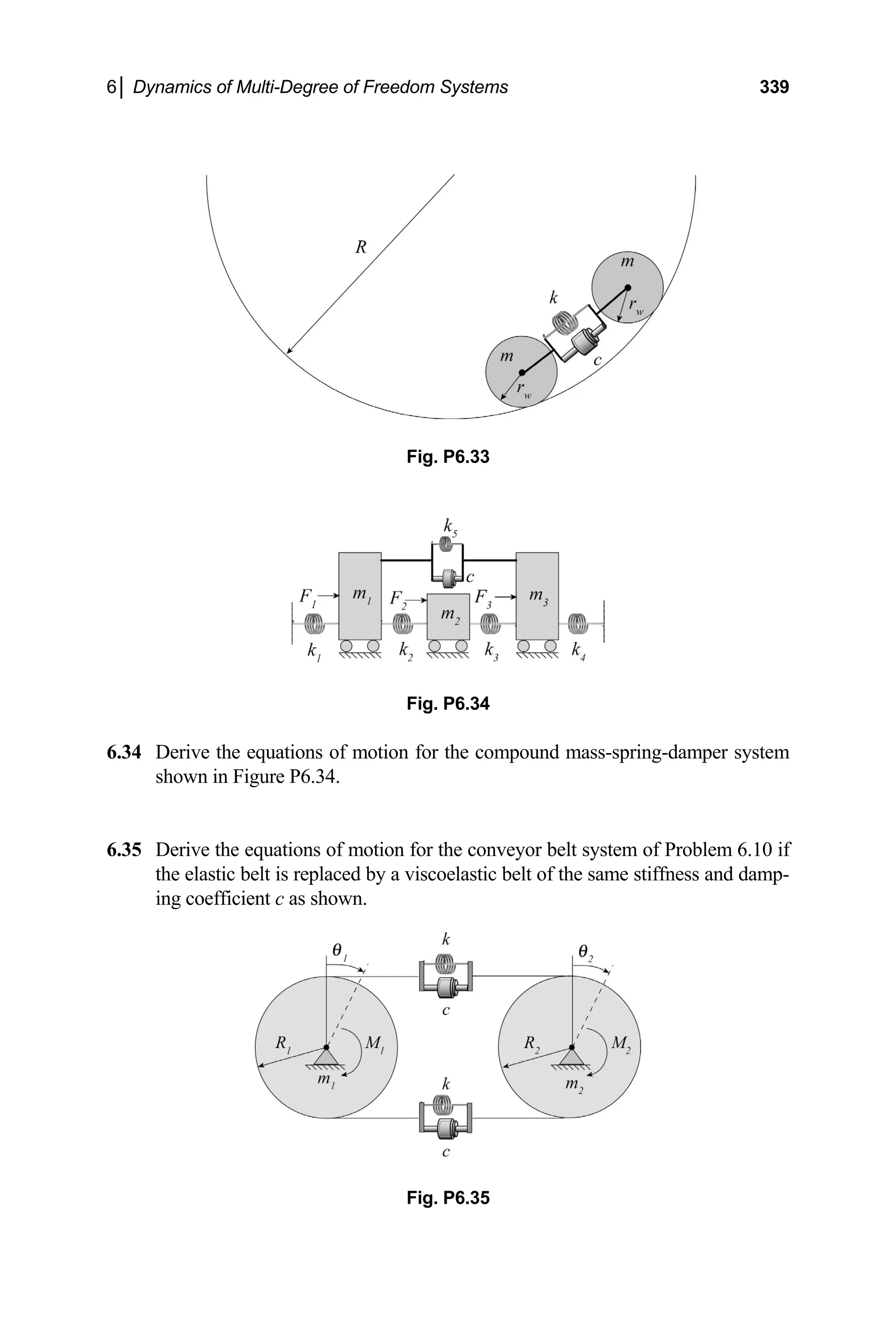
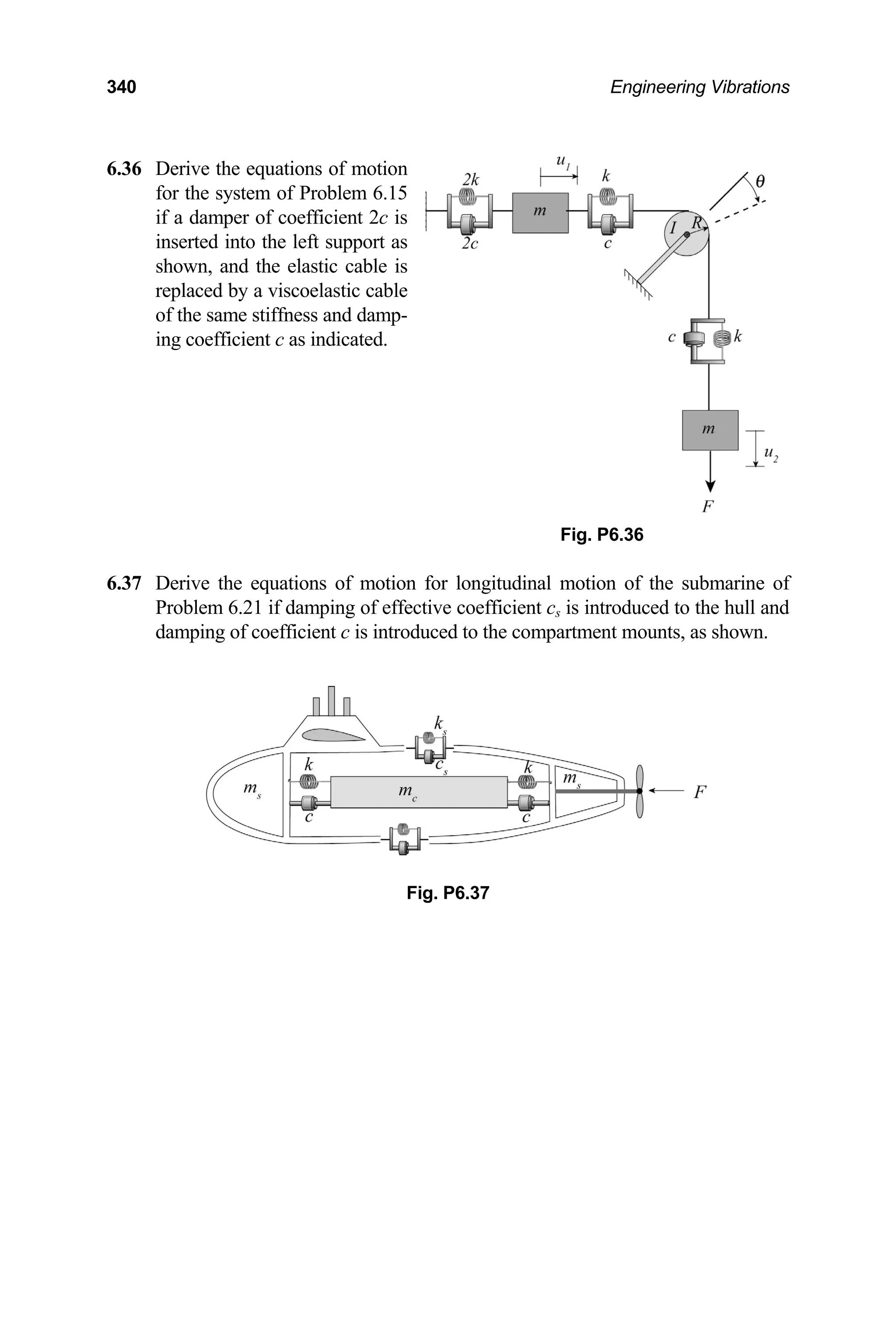
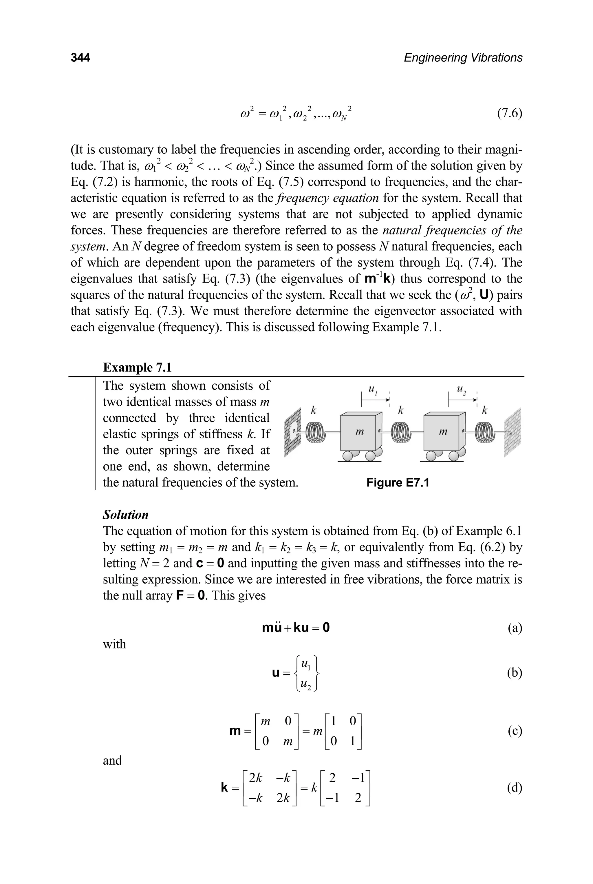
![7│ Free Vibration of Multi-Degree of Freedom Systems 349
Figure E7.2-1 Natural modes of the system depicted in Figure E7.1.
(2) 1
1
1
2
⎧ ⎫
= ⎨ ⎬
−
⎩ ⎭
U (n')
The depictions of the system for each of the modes are shown in Figure E7.2-1.
It may be seen that when the system vibrates in the first mode, it does so at the
frequency 1 k m
ω = , and with both masses moving in the same direction
(left or right) and with the same magnitude. During this motion, the center
spring is unstretched, and so the two masses behave as if they are a single mass
of magnitude 2m as indicated in Figure E7.2-2. The combined stiffness of the
outer spring during this mode is 2k. Thus, for the first mode, the system be-
haves as a single degree of freedom system of mass 2m and stiffness 2k and
hence ω1 is given by Eq. (c-1).
Figure E7.2-2 Effective behavior of system in first mode.
When the system vibrates in the second mode it does so at the frequency
2 3k m
ω = and the motion of the second mass is the reflection of the motion
of the first. When vibrating in this “accordion mode,” the two masses move to-
gether and apart symmetrically about the center of the middle spring. The mid-
point of the center spring remains stationary (and is referred to as a node).
Thus, the motion is equivalent to that of two independent masses of mass m at-
tached to a fixed spring of half the actual length, and hence twice the stiffness
2k [see Eq. (1.8) of Section 1.2.1], as well as to an outer spring of stiffness k as
shown in Figure 7.2-3. This, in turn, is equivalent to two independent masses of](https://image.slidesharecdn.com/engineeringvibrations-240713005818-b85f16c0/75/Engineering-Vibrations-Engineering-Vibrations-371-2048.jpg)
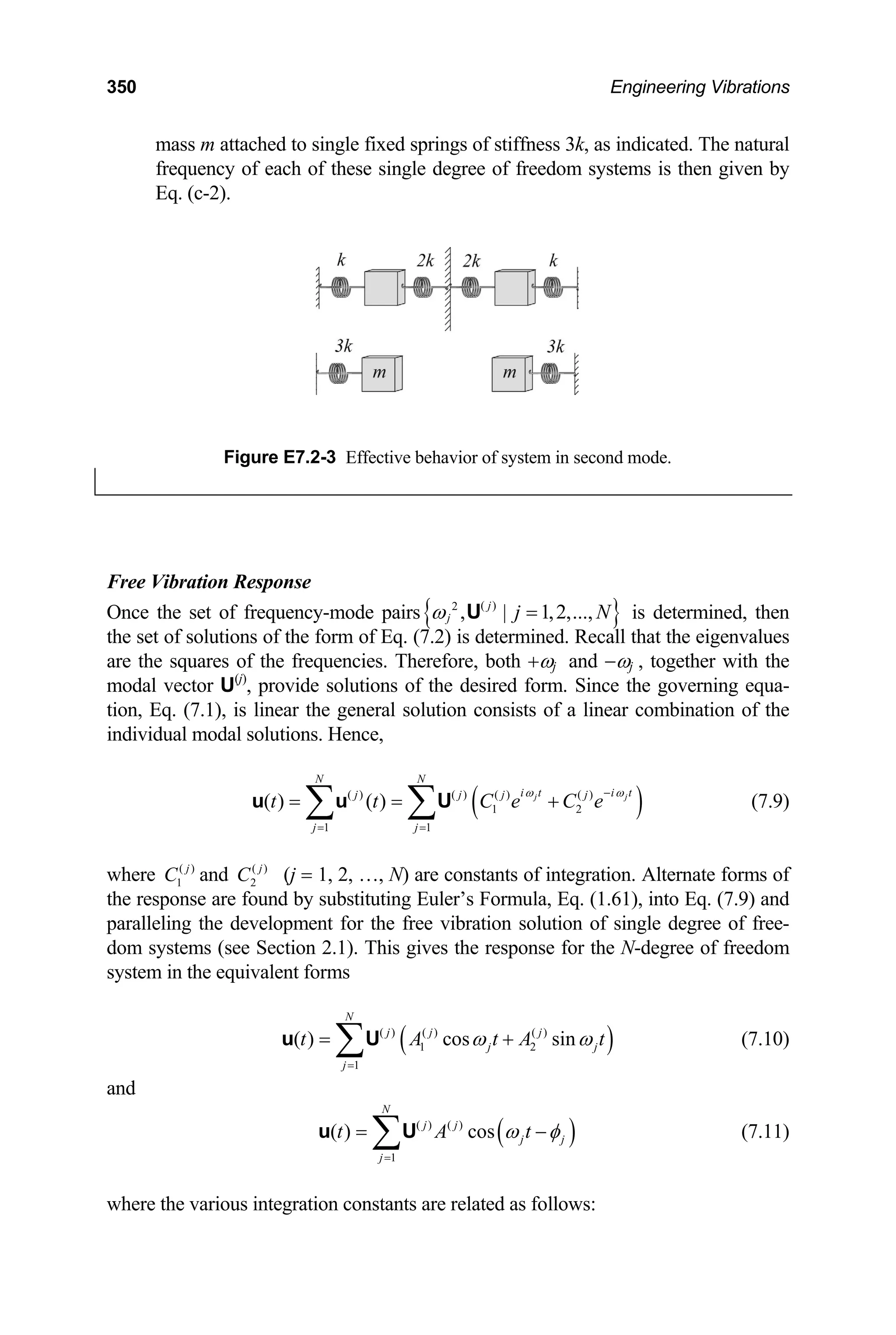
![7│ Free Vibration of Multi-Degree of Freedom Systems 353
The first of Eqs. (i) is satisfied if either A(1)
= 0 or sinφ1 = 0. Since the first of
Eqs. (f) cannot be satisfied if A(1)
= 0, we conclude that
1
sin 0
φ =
and hence that
1 ( 0,1,2,...)
n n
φ π
= = (j)
Similarly, the second of Eqs. (i) is satisfied if either A(2)
= 0 or sinφ2 = 0. How-
ever, the second of Eqs. (f) cannot be satisfied if A(2)
= 0. We thus conclude that
2
sin 0
φ =
and hence that
2 ( 0,1,2,...)
n n
φ π
= = (k)
Substituting Eqs. (j) and (k) into Eqs. (f) we find that,
(1) (2)
(1) (2)
1 2 ( 0,2,4,...)
1 2 ( 1,3,5,...)
A A n
A A n
= = + =
= = − =
(l)
Substitution of Eqs. (l) and (c) into Eq. (b) gives the free vibration response of
the system resulting from the given initial conditions as
1 3
2
( ) 1 1
1 1
( ) cos cos
( ) 1 1
2 2
k
m
u t
t t k
m
u t
⎧ ⎫ ⎧ ⎫ ⎧ ⎫
= = +
⎨ ⎬ ⎨ ⎬ ⎨ ⎬
−
⎩ ⎭ ⎩ ⎭
⎩ ⎭
u t (m)
Equation (m) can also be expressed in the equivalent form
1 3
2
( ) 1 2 1 2
1 1
( ) cos cos
( ) 2 2
1 2 1 2
k k
m m
u t
t t
u t
⎧ ⎫ ⎧ ⎫
⎧ ⎫ ⎪ ⎪ ⎪ ⎪
= = +
⎨ ⎬ ⎨ ⎬ ⎨ ⎬
−
⎩ ⎭ ⎪ ⎪ ⎪ ⎪
⎩ ⎭ ⎩ ⎭
u t (m')
for which the modal vectors have unit magnitude [that is they have the alternate
forms stated by Eqs. (i') and (n') of Example 7.2)]. It may be seen from either
Eq. (m) or Eq. (m') that, for the given initial conditions, the amplitudes of both
modes are the same. Thus, the degree of participation of each mode is the same.
Example 7.4
Consider the system of the previous example when each mass is initially dis-
placed and held a unit distance from its equilibrium position and then both are
released from rest simultaneously. That is, consider an initial displacement of](https://image.slidesharecdn.com/engineeringvibrations-240713005818-b85f16c0/75/Engineering-Vibrations-Engineering-Vibrations-375-2048.jpg)
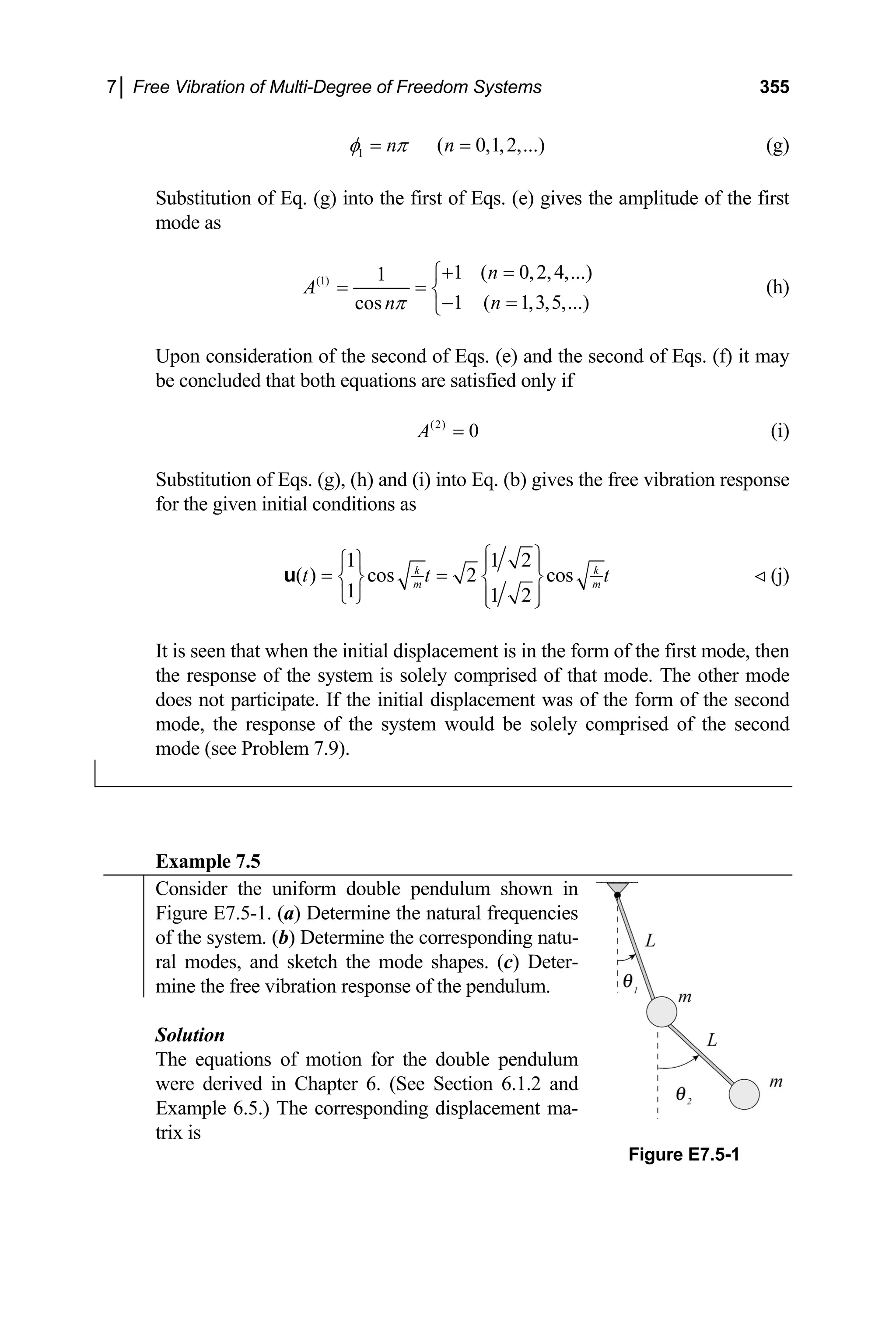
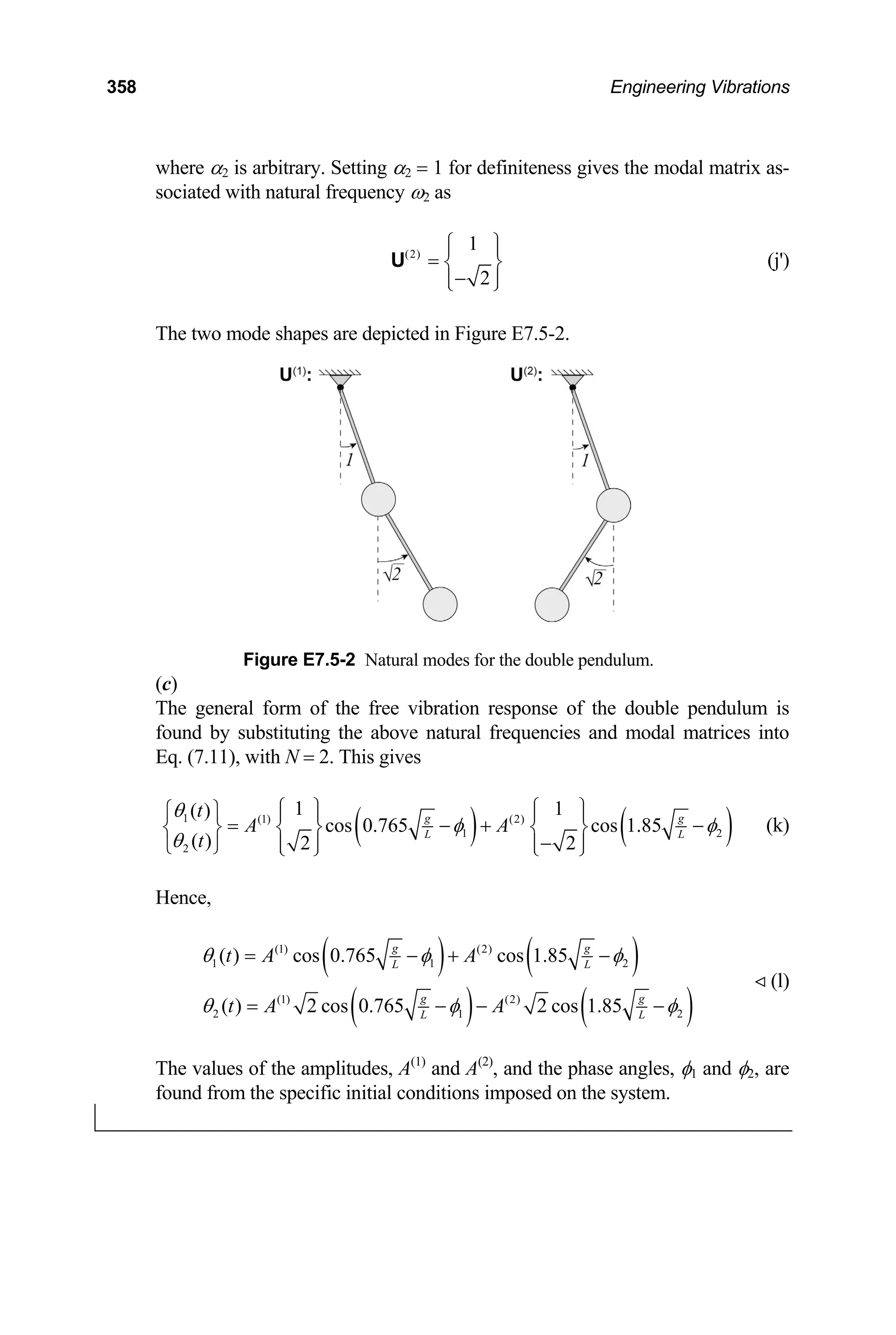
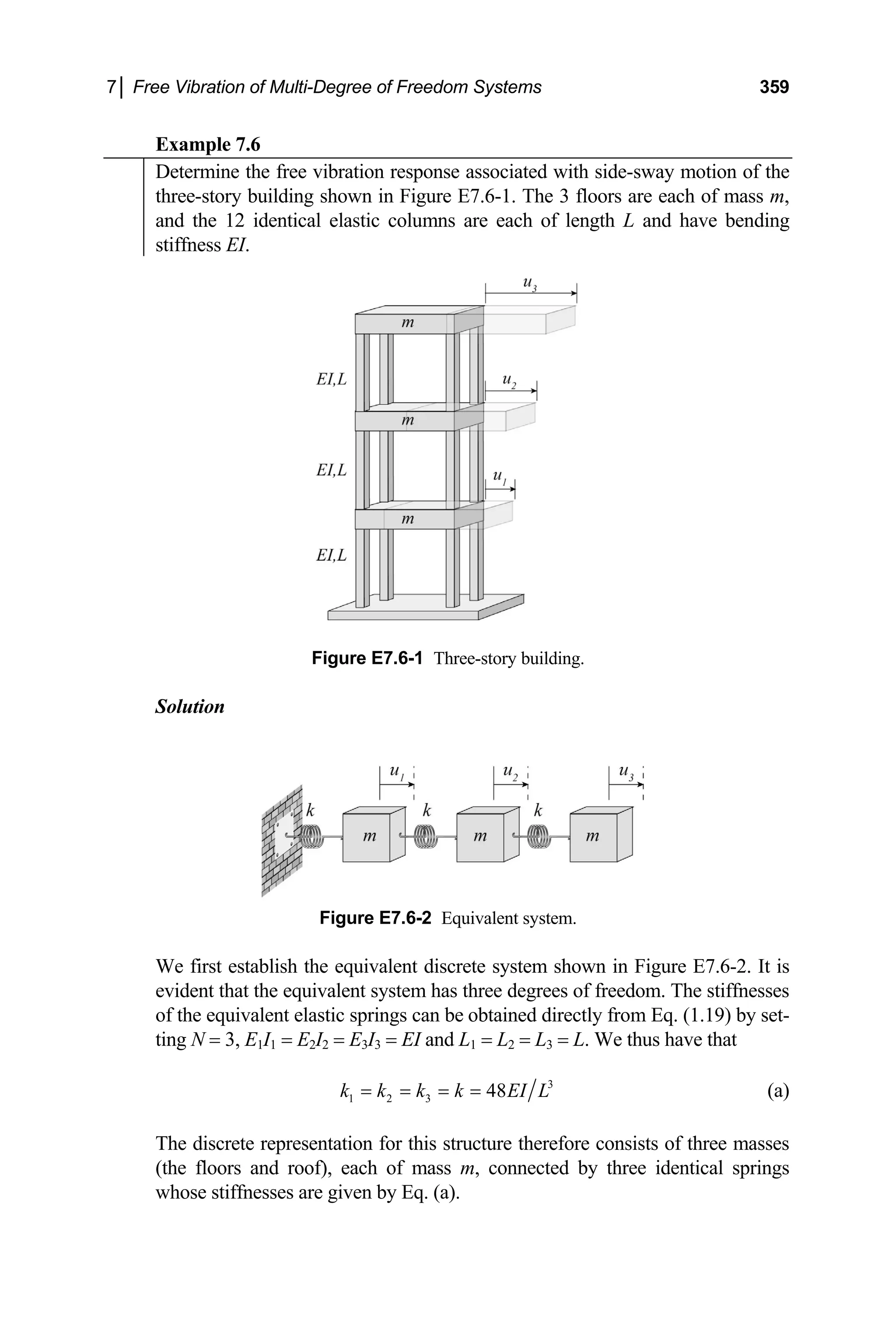
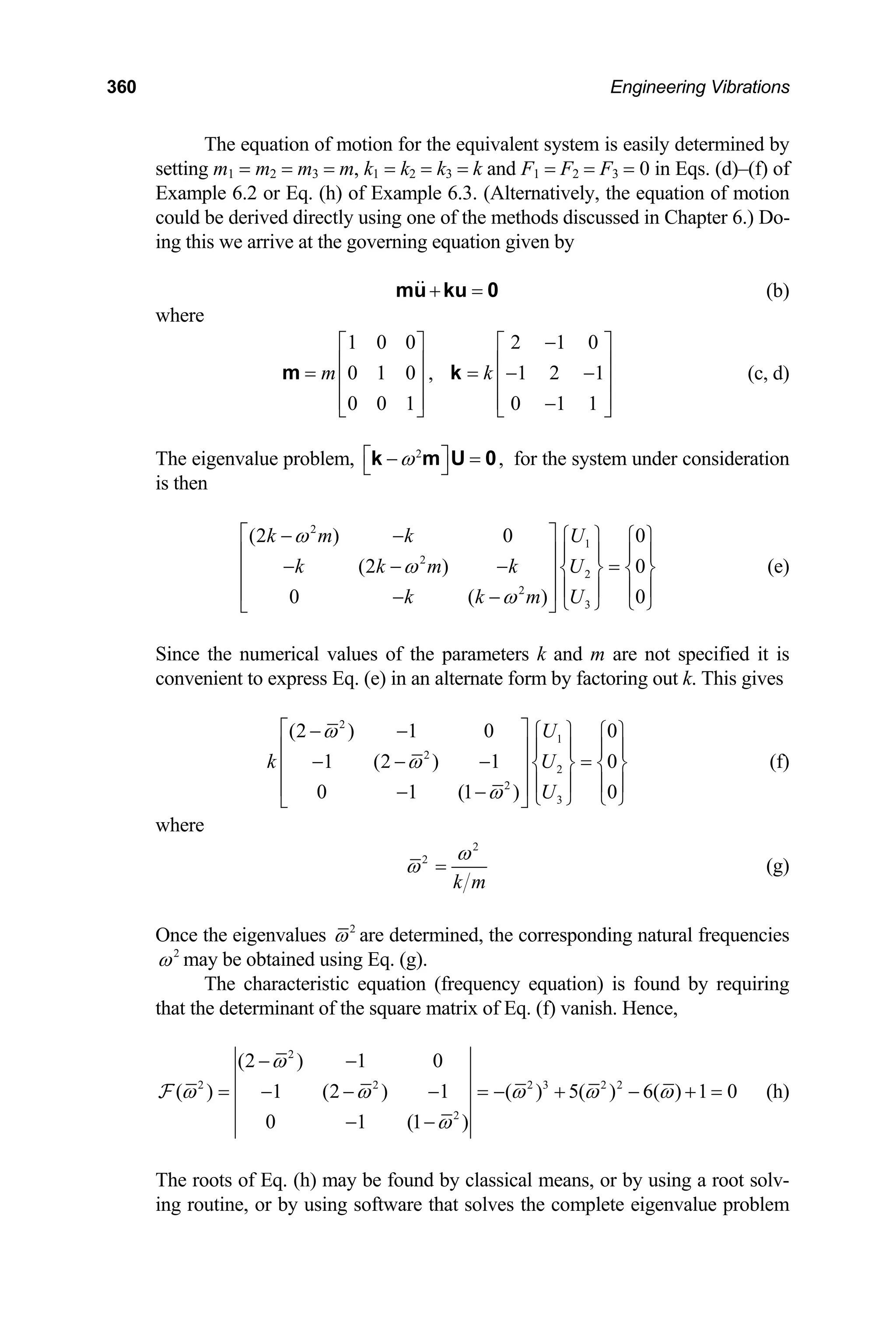
![7│ Free Vibration of Multi-Degree of Freedom Systems 361
defined by Eq. (f) directly, such as the MATLAB function “eig.” We here use the
MATLAB polynomial solver, “roots,” to determine the zeros of the characteris-
tic equation. This is done by constructing the matrix of coefficients of the poly-
nomial appearing in Eq. (h), P = [−1, 5, −6, 1], and invoking the MATLAB com-
mand roots(P). We thus obtain the zeroes of Eq. (h),
2
0.1981, 1.555, 3.247
ω = (i)
Substitution of each eigenvalue of Eq. (i) into Eq. (g) gives the corresponding
natural frequencies for the three-story structure,
1 3
0.4451 3.08
EI
k m
mL
ω = = (j-1)
2 3
1.247 8.64
EI
k m
mL
ω = = (j-2)
3 3
1.802 12.5
EI
k m
mL
ω = = (j-3)
To determine the associated modal vectors, we substitute a frequency from Eq.
(j), or equivalently Eq. (i), into Eq. (f) and solve for the components of the cor-
responding modal vector. Since the matrix 2
ω
⎡ ⎤
− =
⎣ ⎦
k m U 0 was rendered sin-
gular by requiring that its determinant vanish, (at most) only two of the three
scalar equations of Eq. (f) will be independent. We shall choose to solve the
first and third equations since they each have a vanishing term. Hence,
2 ( ) ( )
1 2
( ) 2 ( )
2 3
(2 ) 0
(1 ) 0
j j
i
j j
i
U U
U U
ω
ω
− −
− + − =
=
( 1,2,3)
j = (k)
(1)
U :
Substitution of the first value of Eq. (i) into Eqs. (k), with j = 1, gives
(1) (1) (1) (1)
1 2 2 1
(2 0.1981) 0 1.802
U U U U
− − = ⇒ =
(1) (1) (1) (1) (1)
2 3 3 2
(1 0.1981) 0 1.247 2.247
U U U U
− + − = ⇒ = = 1
U
Hence,
(1)
1
1
1.802
2.247
α
⎧ ⎫
⎪ ⎪
= ⎨ ⎬
⎪ ⎪
⎩ ⎭
U (l)
where α1 is an arbitrary scalar. The scalar multiplier can be chosen as anything
we like, such as unity as was done in prior examples. For this case, however,](https://image.slidesharecdn.com/engineeringvibrations-240713005818-b85f16c0/75/Engineering-Vibrations-Engineering-Vibrations-383-2048.jpg)
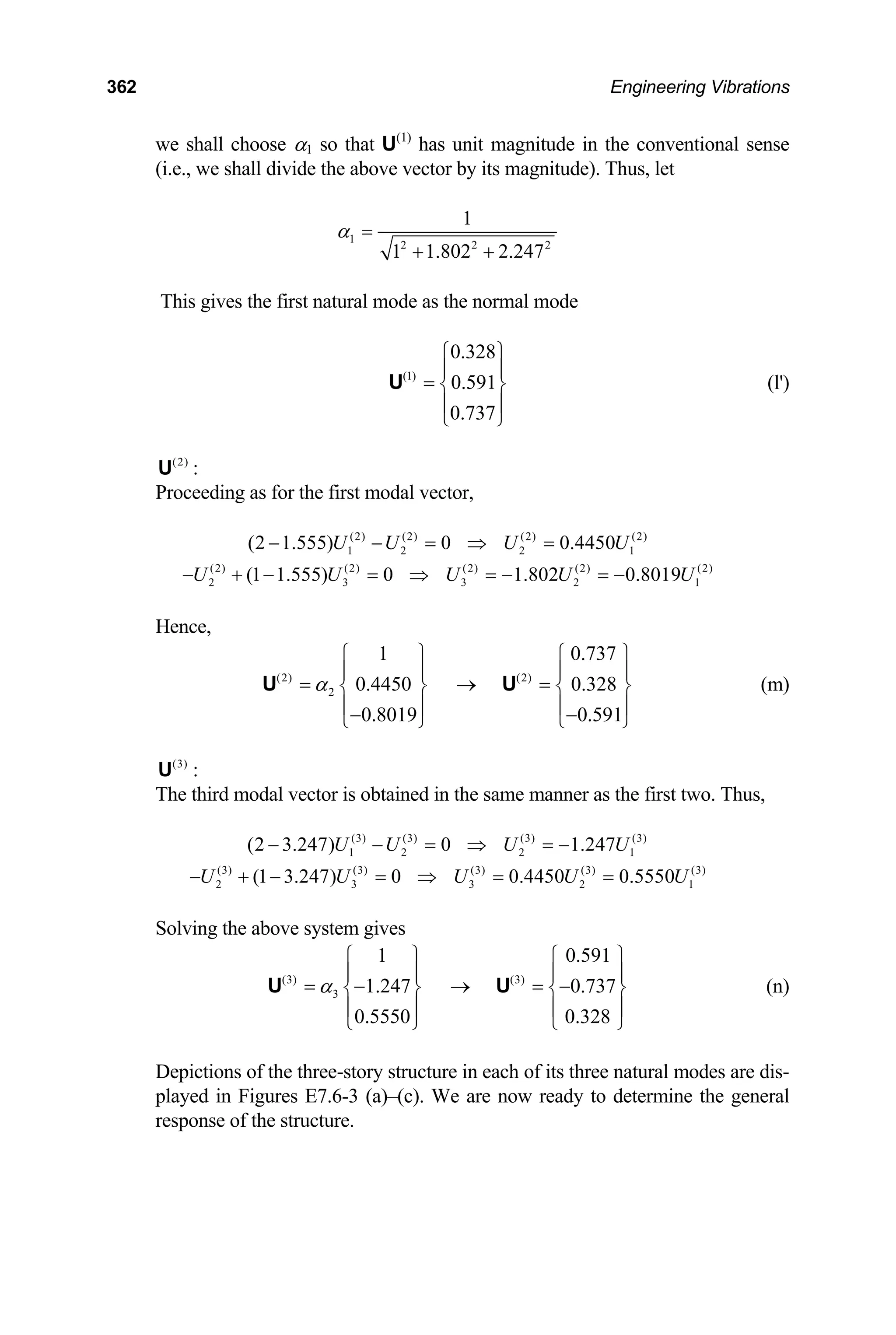
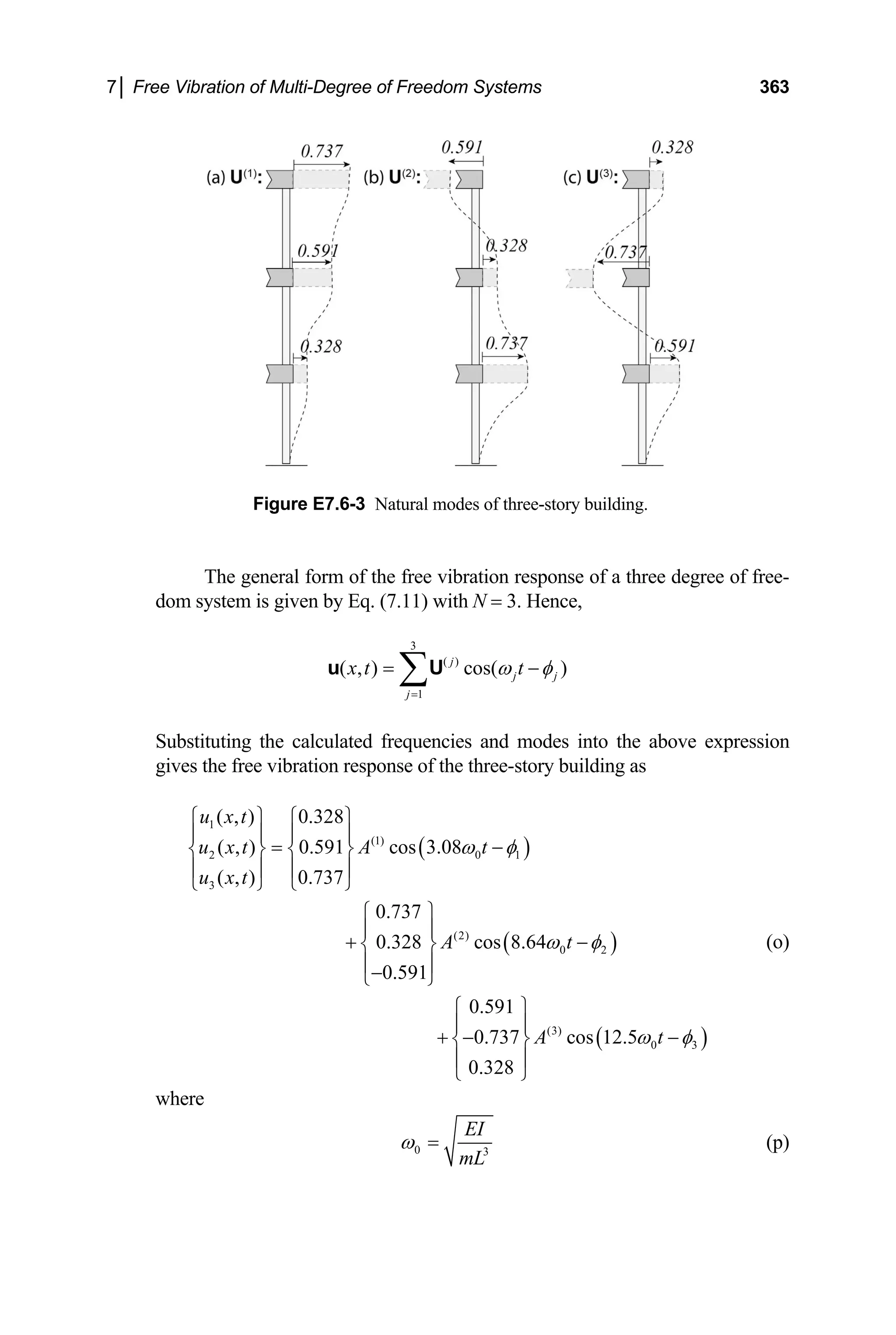
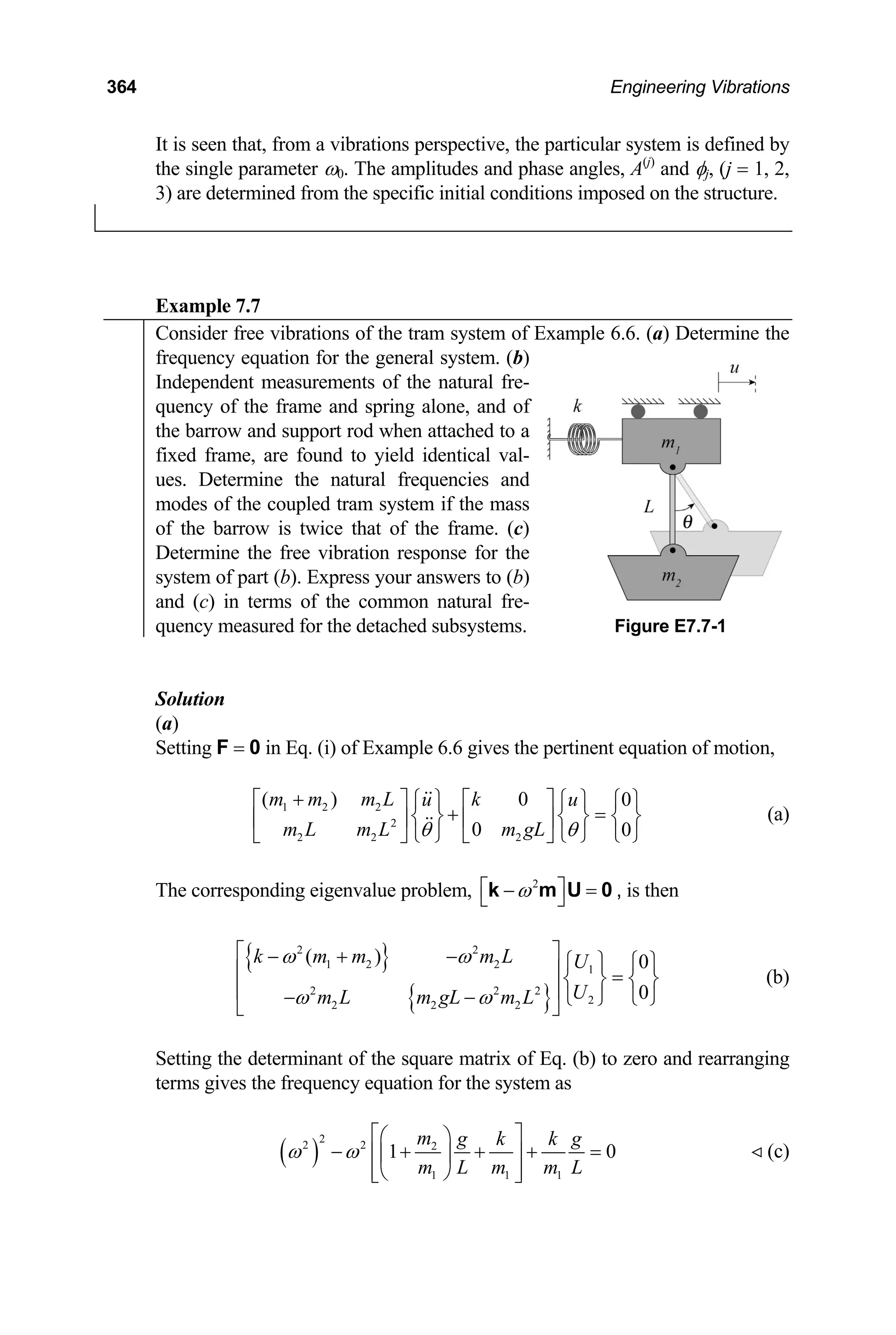
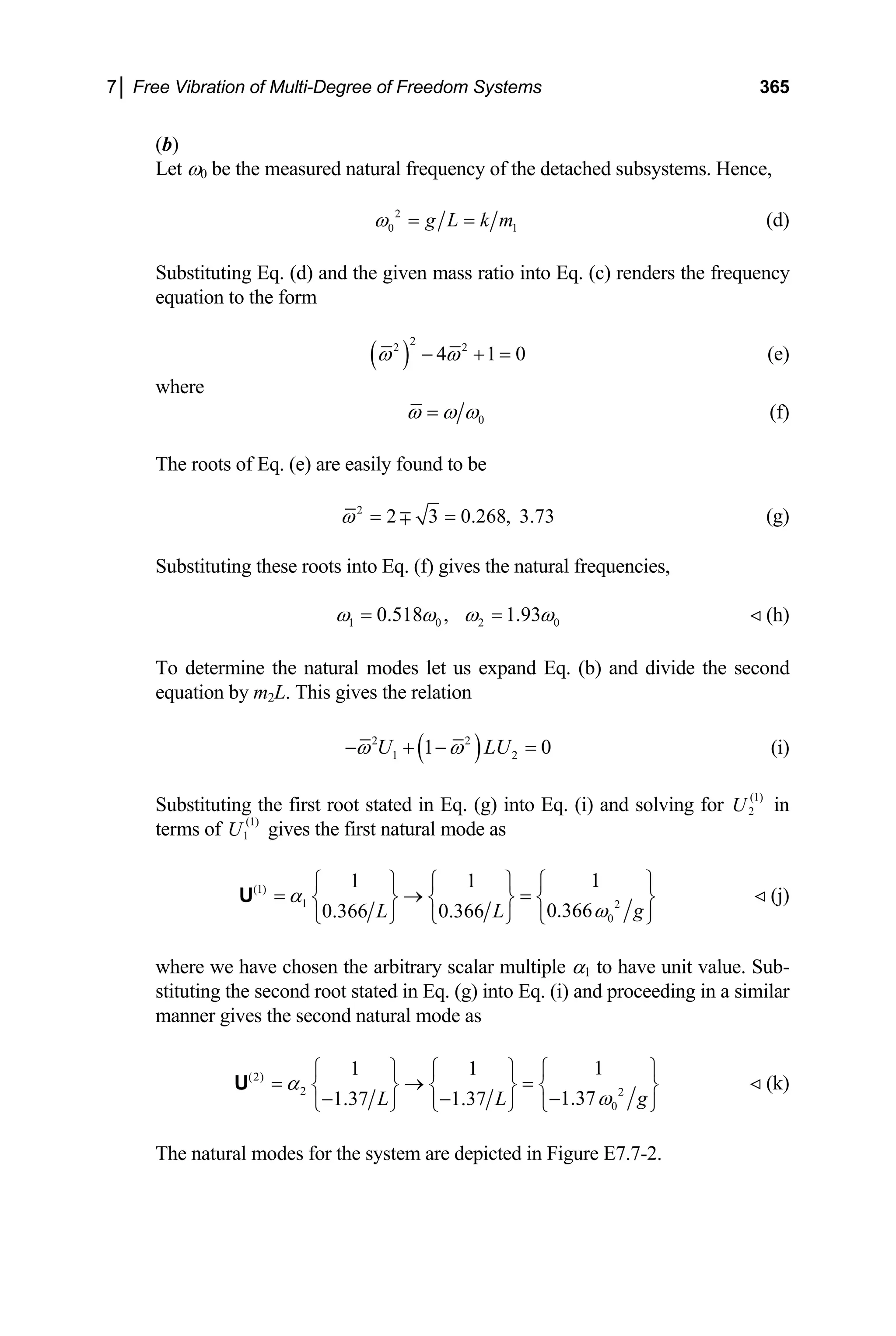
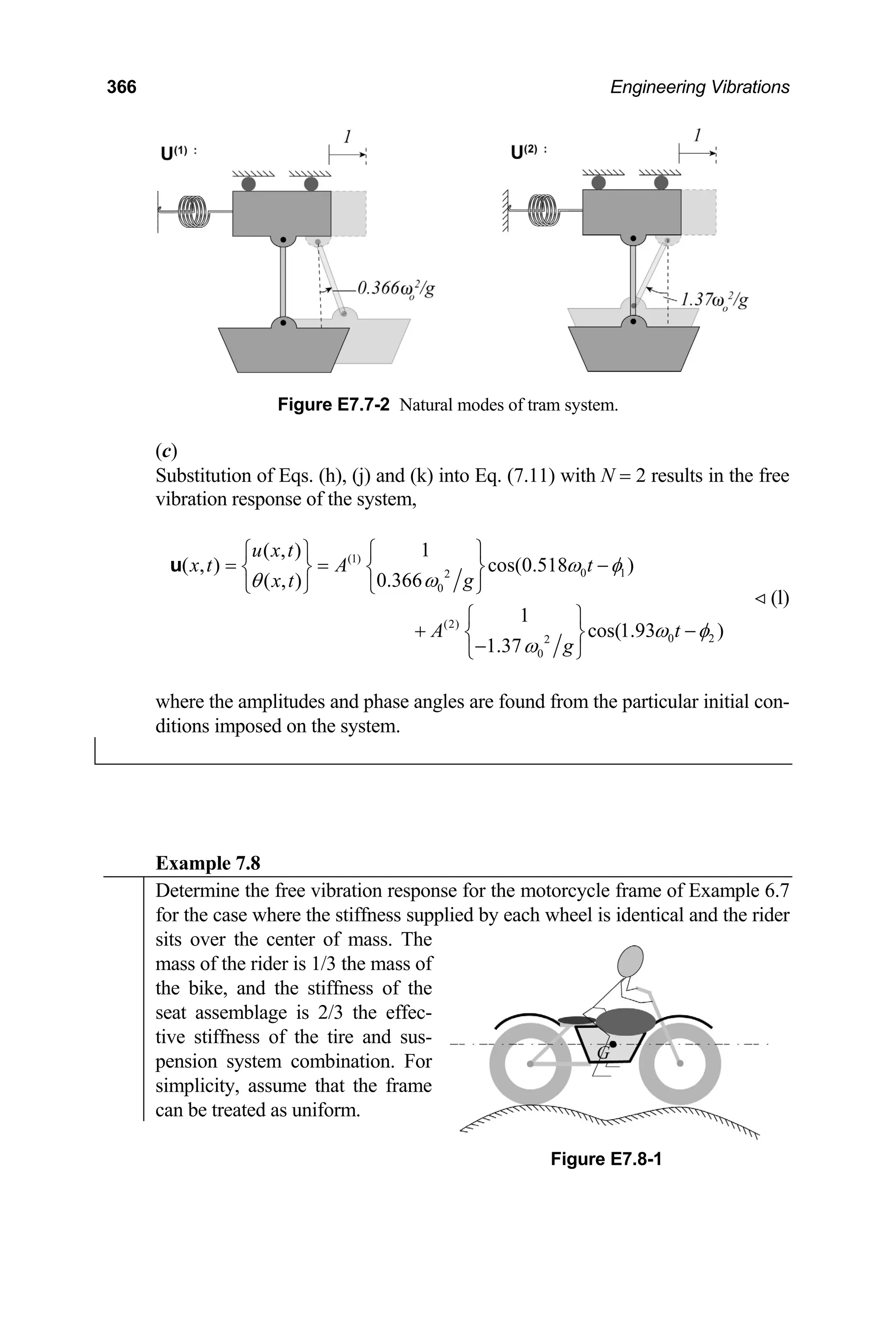
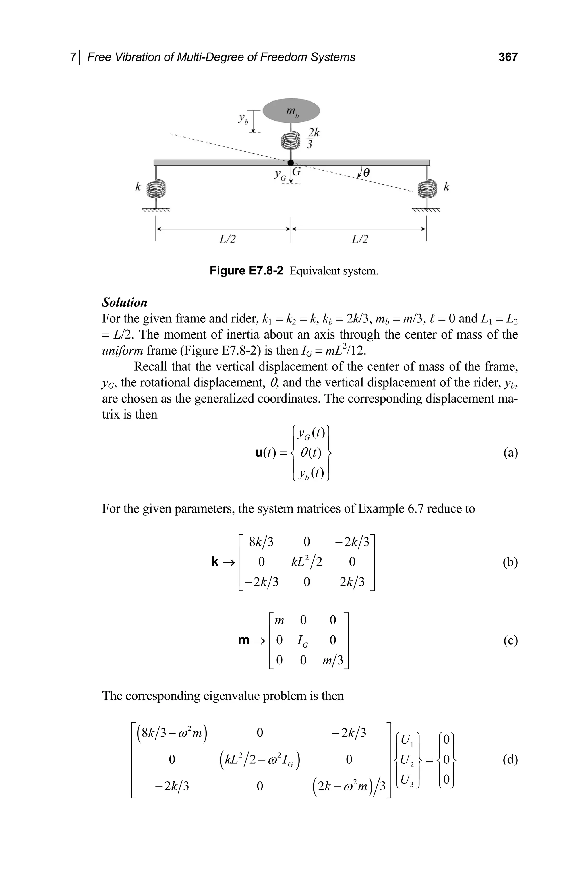
![368 Engineering Vibrations
We next determine the frequency equation for the system. Hence,
( )
( )
( )
2
2 2
2
8 3 0 2 3
0 2 0
2 3 0 2 3
G
k m k
kL I
k k
ω
ω
ω
− −
0
m
− =
− −
(e)
Expanding the above determinant gives the desired frequency equation,
( )
2 2 2 2 2 2 2
2 12 4 ( ) 3 ( )
G
kL I k k m m
ω ω ω
⎡
− −1 +
⎣ 0
⎤ =
⎦ (f)
Equation (f) is easily factored to yield the natural frequencies,
2 2 2 2
1 2 3
1.132 , 3.535 , 2 6
G
k m k m kL I k m
ω ω ω
= = = = (g)
We next determine the associated modal vectors. Substituting the first fre-
quency into the first row of Eq. (d) gives
8
1.132
3
k
k
m
− m (1) (1) (1) (1)
1 3 3
2
0 2.303
3
U kU U U
⎛ ⎞
− = ⇒ =
⎜ ⎟
⎝ ⎠
1 (h)
[The third row of Eq. (d) gives the identical relation.] Substituting the first
natural frequency into the second row of Eq. (d) gives
2 k 2
1.132
k
L −
m
m (1) (1)
2 0 0
U U
⎛ ⎞
2
= ⇒ =
⎜ ⎟
⎝ ⎠
(i)
Combining Eqs. (h) and (i) in matrix form gives the modal vector associated
with the first natural frequency,
(1)
1
0
2.303
⎧ ⎫
⎪ ⎪
= ⎨ ⎬
⎪ ⎪
⎩ ⎭
U (j)
A physical depiction of the modal vector is shown in Figure E7.8-3a. Similar
calculations give the modal vector associated with the second natural fre-
quency. Hence,](https://image.slidesharecdn.com/engineeringvibrations-240713005818-b85f16c0/75/Engineering-Vibrations-Engineering-Vibrations-390-2048.jpg)
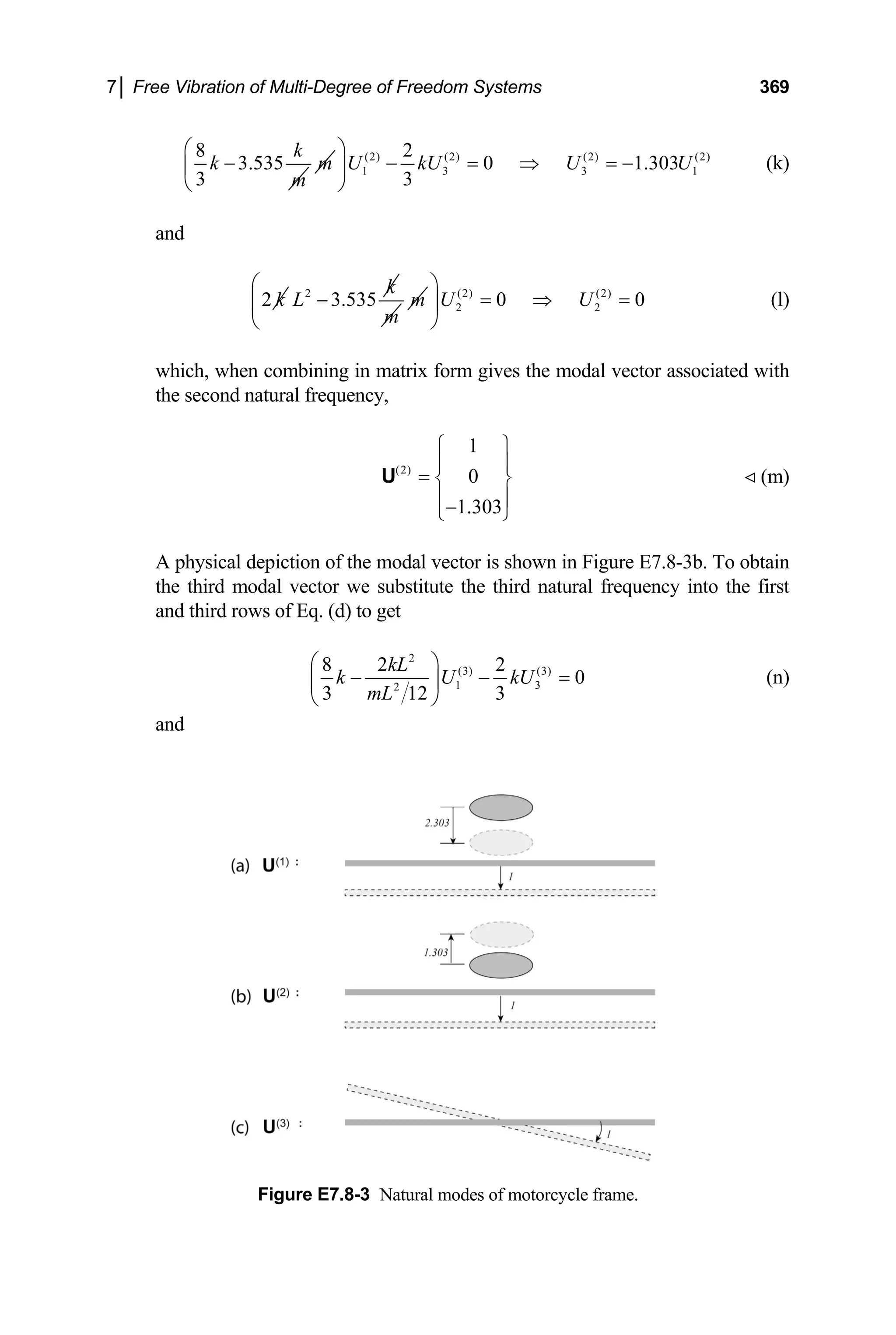
![370 Engineering Vibrations
2
(3) (3)
1 2
2 2
2
3 12
mL
kU U
mL
⎛ ⎞
− + −
⎜ ⎟
⎝ ⎠
3 0
= (o)
These two equations may be solved to give
(3) (3)
1 3 0
U U
= = (p)
Since Eqs. (n) and (o) yielded definite values, the second row of Eq. (d) will re-
flect the lack of determinacy. Substituting the third natural frequency into the
second row of Eq. (d) gives the relation
2
2 2
2
G
kL
kL
I
− G
I (3) (3) (3)
2 2 2
0 0 0
U U U anything
⎛ ⎞
⎜ ⎟ = → ⋅ = ⇒ =
⎜ ⎟
⎝ ⎠
(q)
as we would expect since the square matrix of Eq. (d) must be singular. [For
this frequency, all elements of the second row of the square matrix of Eq. (d)
vanish.] The third modal vector is thus of the form
(3)
0
1
0
⎧ ⎫
⎪ ⎪
= ⎨ ⎬
⎪ ⎪
⎩ ⎭
U (r)
As seen in the depiction of the mode shown in Figure E7.8-3c, the third mode
corresponds to pure rotation. Finally, the free vibration response of the motor-
cycle frame is
( )
( )
(1)
0 1
(2)
0 2
(3)
0
( ) 1
( ) 0 cos 1.06
( ) 2.30
1
0 cos 1.88
1.30
0
1 cos 2.45
0
G
b
y t
t A t
y t
A t
A t
θ ω φ
ω φ
ω
⎧ ⎫ ⎧ ⎫
⎪ ⎪ ⎪ ⎪
= −
⎨ ⎬ ⎨ ⎬
⎪ ⎪ ⎪ ⎪
⎩ ⎭ ⎩ ⎭
⎧ ⎫
⎪ ⎪
+ −
⎨ ⎬
⎪ ⎪
−
⎩ ⎭
⎧ ⎫
⎪ ⎪
+ −
⎨ ⎬
⎪ ⎪
⎩ ⎭
( )
3
φ
(s)
where
0 k m
ω = (t)](https://image.slidesharecdn.com/engineeringvibrations-240713005818-b85f16c0/75/Engineering-Vibrations-Engineering-Vibrations-392-2048.jpg)
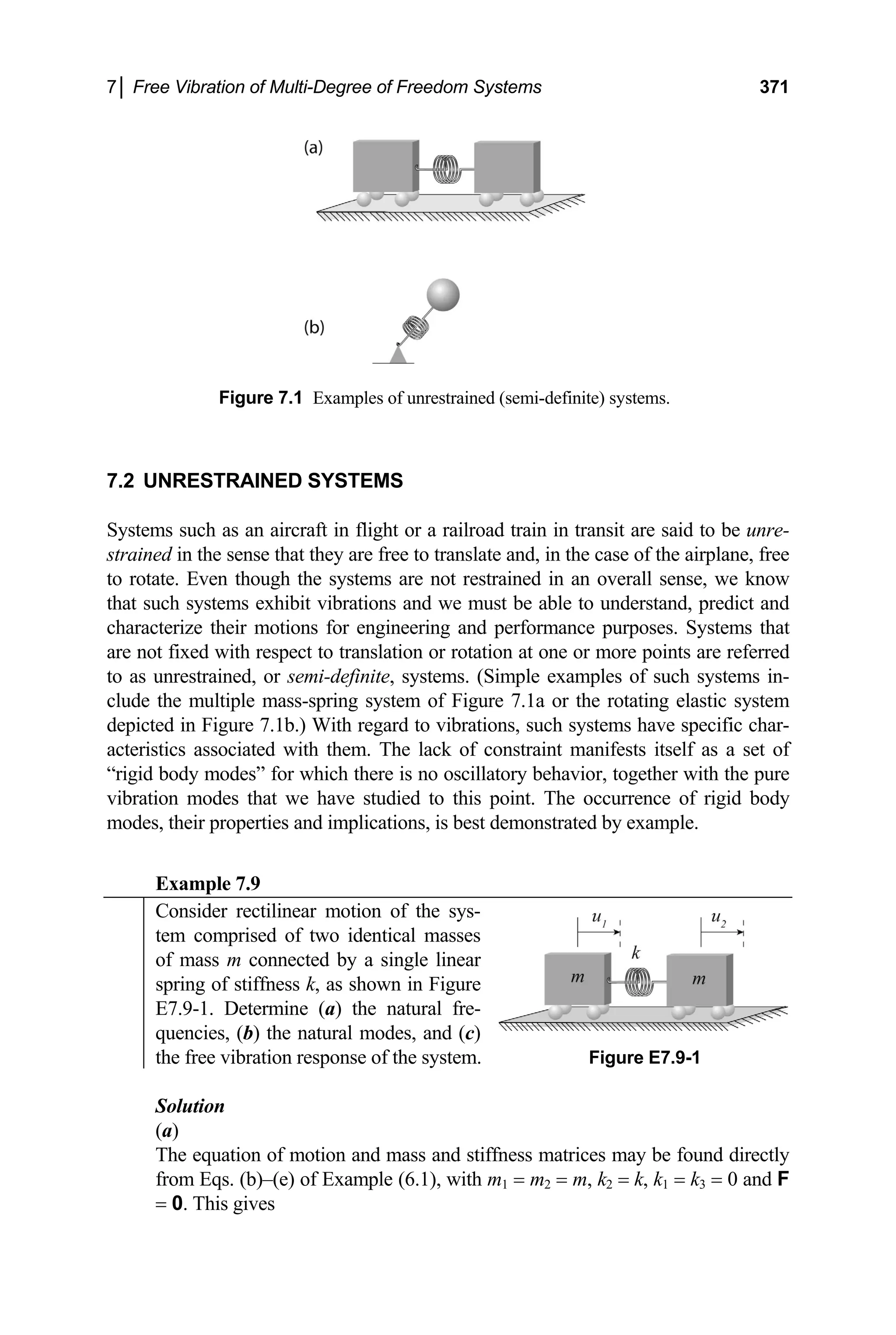
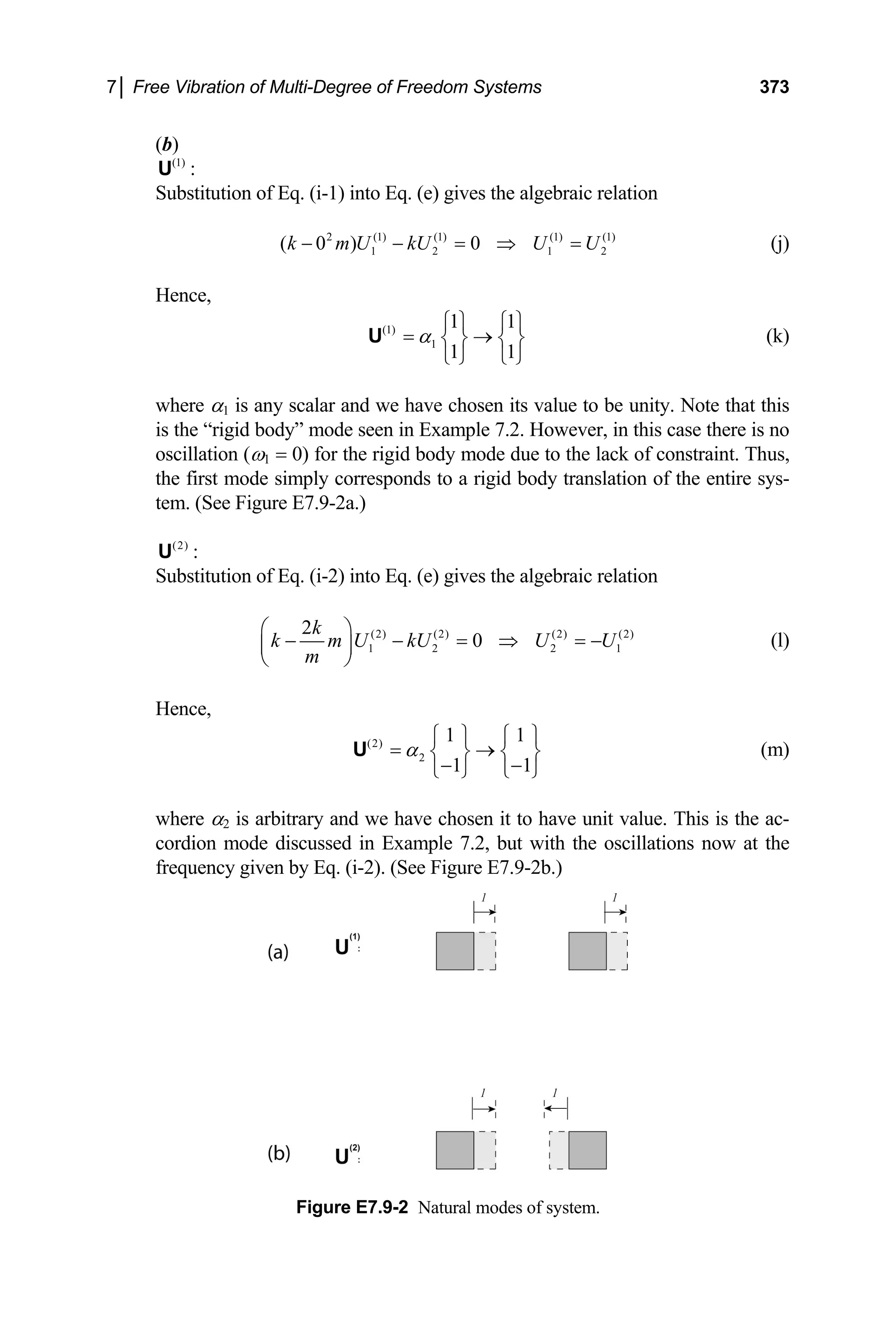
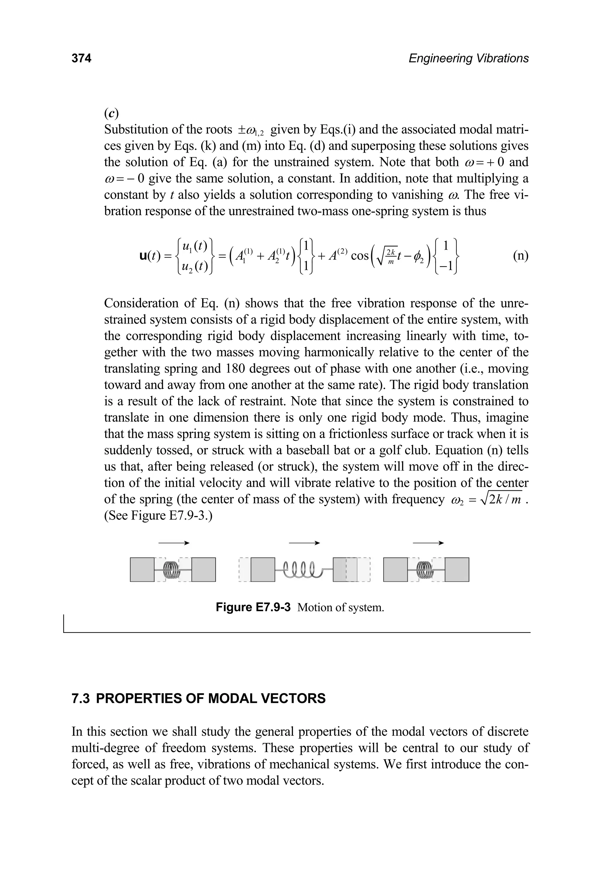
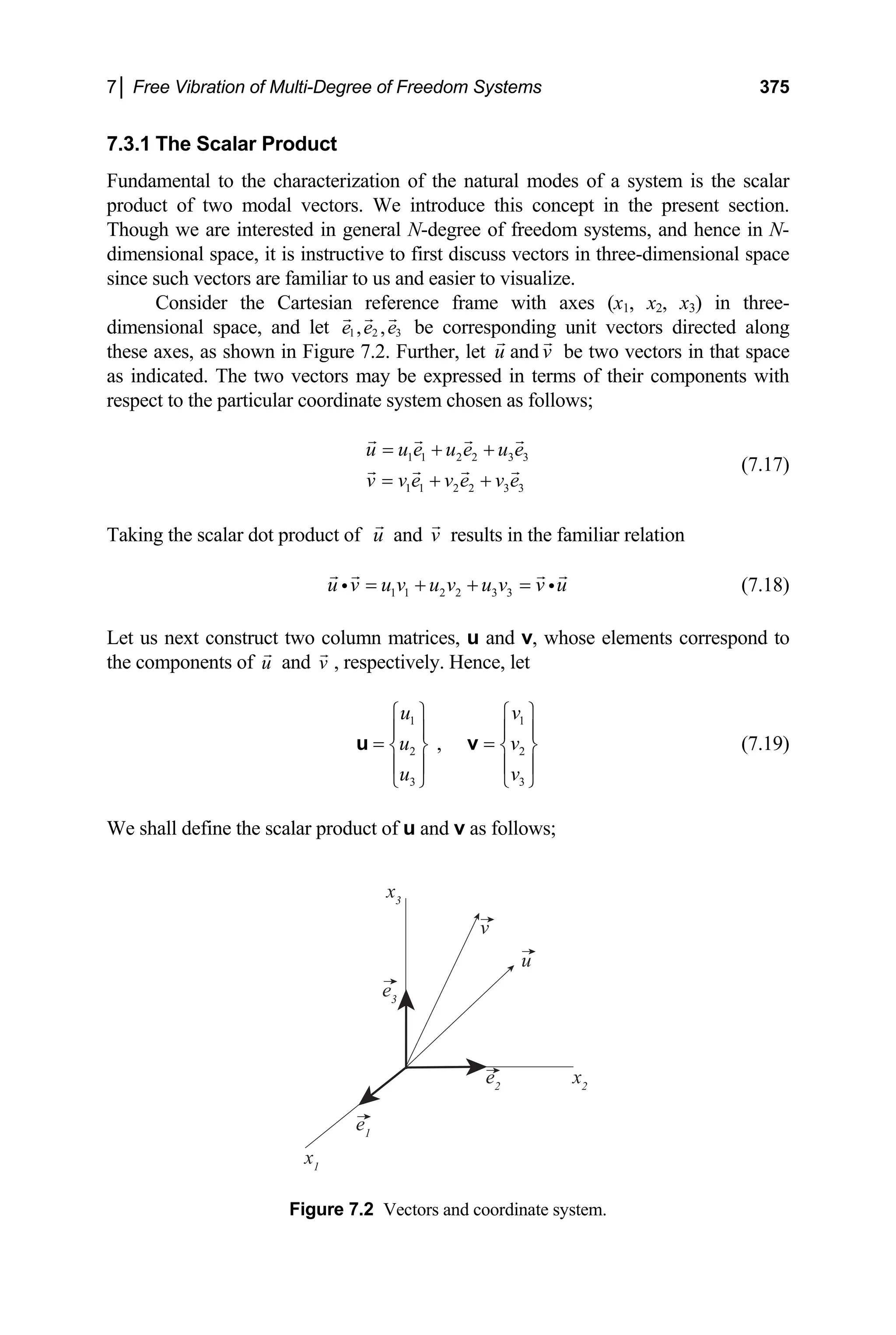
![376 Engineering Vibrations
[ ]
1
1 2 3 2 1 1 2 2 3 3
3
, ,
v
u u u v u v u v u v
v
⎧ ⎫
⎪ ⎪
≡ = = + + = =
⎨ ⎬
⎪ ⎪
⎩ ⎭
u v u v v u v u
T T
(7.20)
Comparison of Eqs. (7.20) and (7.18) shows the two to be equivalent statements.
Orthogonality
The basic definition and geometric interpretation of the scalar dot product between
two vectors is given by the relation
cos
u v u v θ
=
i (7.21)
where θ is the angle between the vectors. It follows that
if 0 then
u v u v
= ⊥
i (7.22)
Likewise, we say that,
if , 0
=
u v then ⊥
u v .
The Weighted Scalar Product
It is useful for our study of vibrations, as well as for fundamental purposes, to extend
the concept of the scalar product beyond the elementary definition and operation dis-
cussed above. Therefore, let us consider some square symmetric matrix A = AT
and
two column matrices u and v. The weighted scalar product of u and v with respect to
the weight matrix A is defined as
, ≡
A
u v u Av
T
(7.23)
The operation described by Eq. (7.23) may be interpreted algebraically as taking a
scalar product of the two vectors u and v, but weighting the contributions of the vari-
ous products of the elements (components) differently according to the weight matrix
A. The operation may be interpreted geometrically as first stretching and rotating the
vector v to obtain a new vector ,
=
v Av then taking the conventional dot product
between the vectors u and .
v Orthogonality of two vectors with respect to the weight
matrix is defined accordingly.](https://image.slidesharecdn.com/engineeringvibrations-240713005818-b85f16c0/75/Engineering-Vibrations-Engineering-Vibrations-398-2048.jpg)
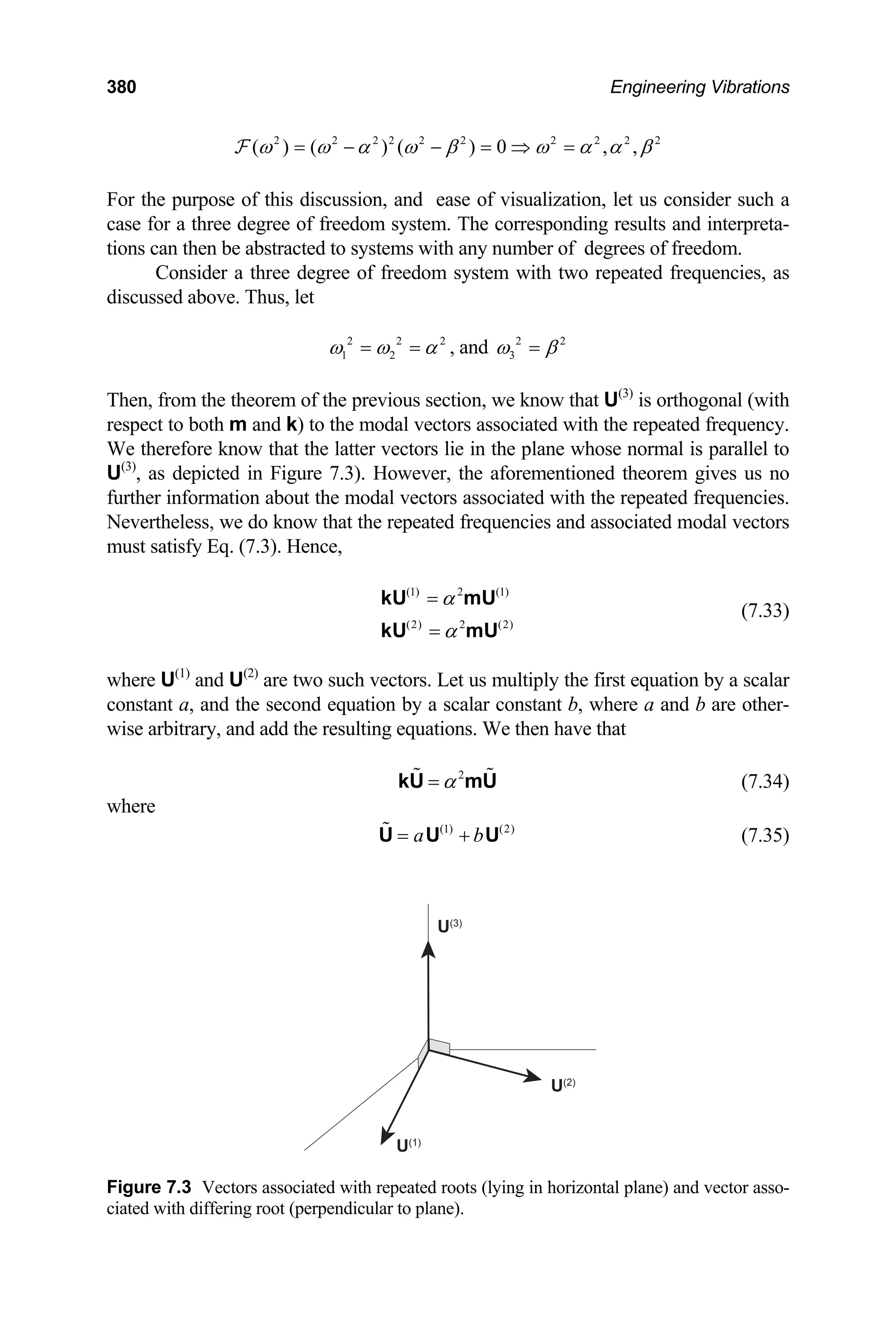
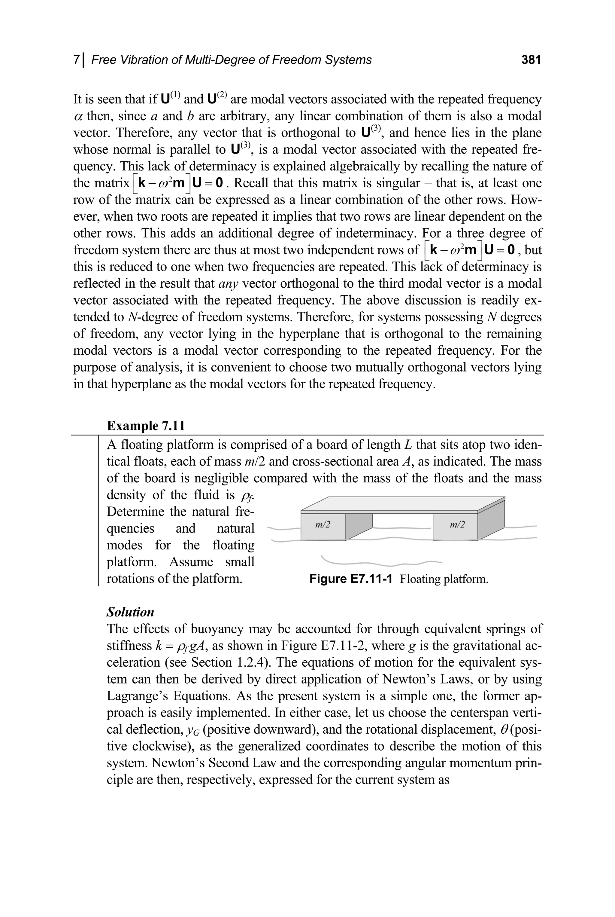
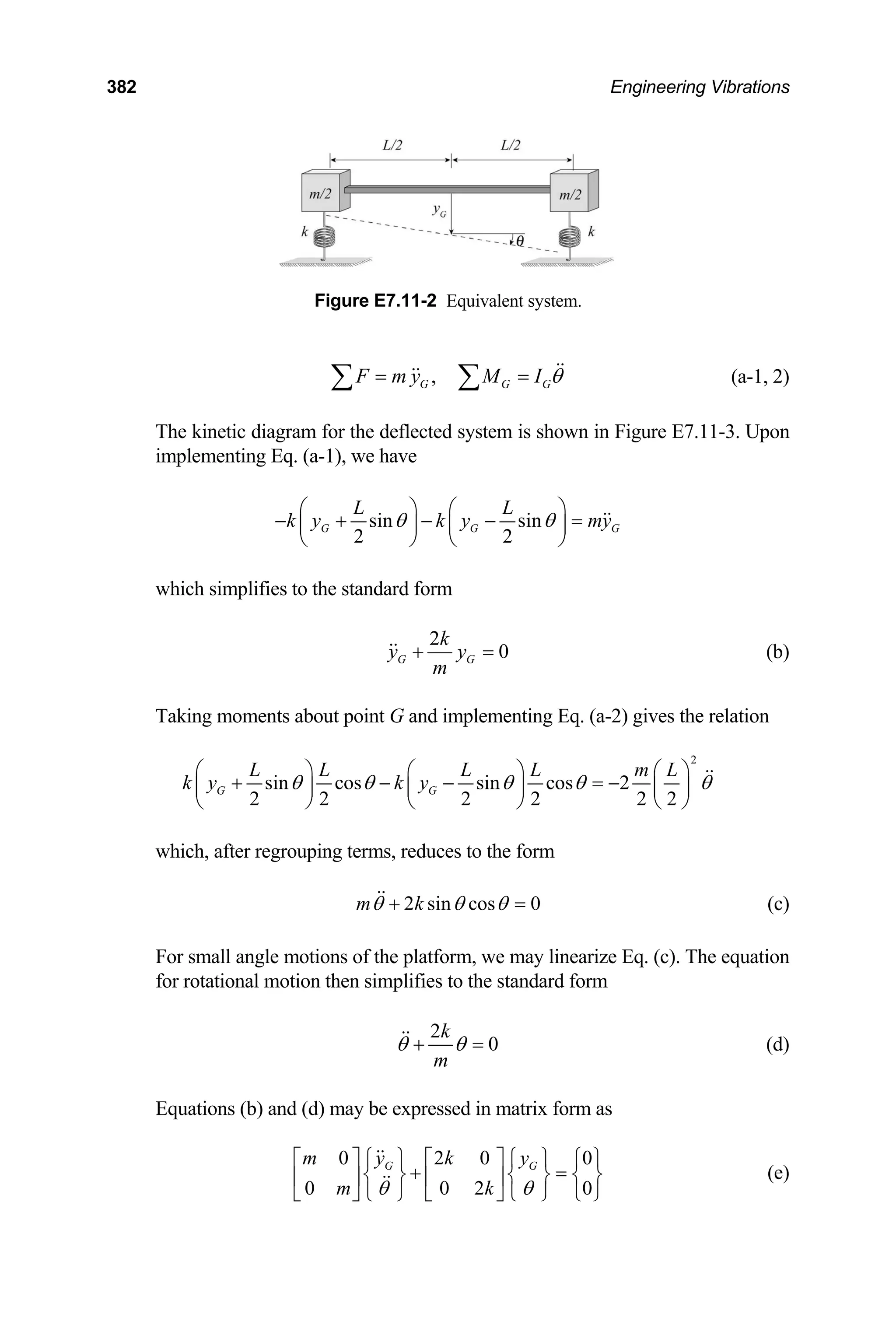
![7│ Free Vibration of Multi-Degree of Freedom Systems 383
Figure E7.11-3 Kinetic diagram.
A comparison of the equations for translational and rotational motion, Eqs. (b)
and (d), reveals two interesting properties of the system. First, we may note that
the two equations are uncoupled for the chosen generalized coordinates. (Coor-
dinates which have this property are referred to as principal, or modal, coordi-
nates and will be discussed formally in the next chapter.) Second, it is readily
seen that
1 2
2k
m
ω ω
= = (f)
That is, the natural frequencies for the two motions are the same. Formally, the
eigenvalue problem for this system takes the form
2
2
0
(2 ) 0
0
0 (2 )
Y
k m
k m
ω
ω
⎡ ⎤ ⎧ ⎫ ⎧ ⎫
−
=
⎨ ⎬ ⎨ ⎬
⎢ ⎥
Θ
− ⎩ ⎭ ⎩ ⎭
⎣ ⎦
(g)
The corresponding frequency equation is then
2 2 2
( ) det (2 ) 0
k m
ω ω ω
⎡ ⎤ 2
= − = − =
⎣ ⎦
k m
F (h)
which yields the roots
2 2 2
,
k k
m m
ω = (i)
The roots of the frequency equation are clearly repeated (not distinct) and, of
course, yield the identical frequencies stated in Eq. (f).
To determine the modal matrices we substitute the frequencies into Eq.
(g) and solve for U(j)
= [Y(j)
Θ(j)
]T
(j = 1, 2). Since the roots are repeated (the
two natural frequencies are the same) this gives, for both modes,](https://image.slidesharecdn.com/engineeringvibrations-240713005818-b85f16c0/75/Engineering-Vibrations-Engineering-Vibrations-405-2048.jpg)
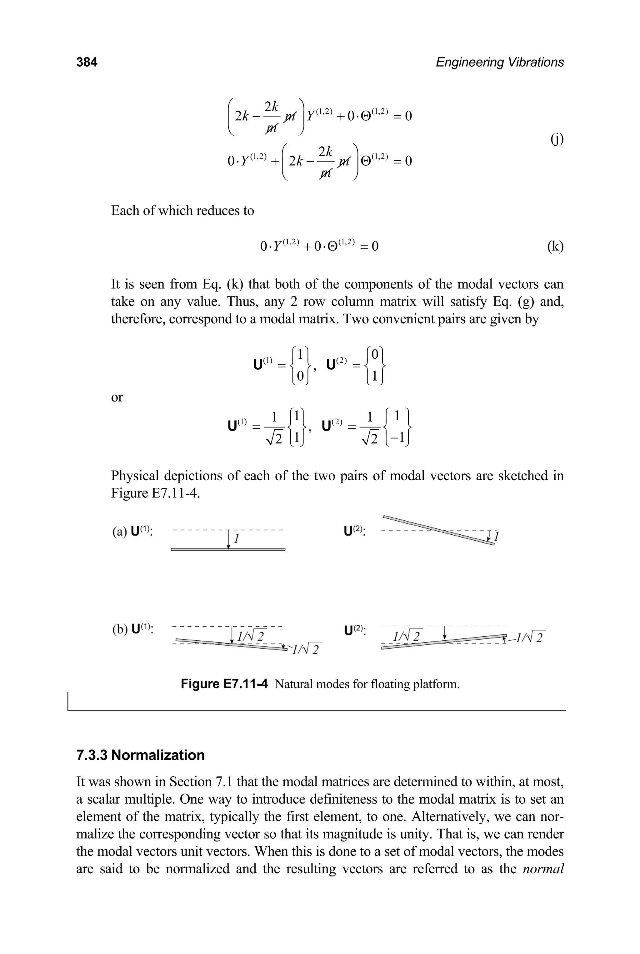
![7│ Free Vibration of Multi-Degree of Freedom Systems 385
modes of the system. In the present section, we shall discuss several options for con-
structing a set of normal modes.
A unit vector is a vector whose scalar product with itself is one. In this regard,
the scale or metric may be defined in several ways. We can set the conventional sca-
lar product of a modal vector with itself to unity, or we can set a weighted scalar
product of the modal vector with itself to unity. For the latter case we have two obvi-
ous candidates for the weight matrix; the mass matrix or the stiffness matrix. The
problem may be stated mathematically as follows; since a modal matrix is determined
to within a scalar multiplier, a typical modal vector for an N-degree of freedom sys-
tem will be of the form
1
2
N
U
U
U
α
⎧ ⎫
⎪ ⎪
⎪ ⎪
= ⎨ ⎬
⎪ ⎪
⎪ ⎪
⎩ ⎭
U (7.36)
here α is arbitrary. To construct the corresponding normal mode, we take the scalar
Conventional Scalar Product
in terms of the conventional scalar product, we take
w
product of this vector with itself, set the resulting expression to one and solve for α.
Then, substitute the calculated value of α back into Eq. (7.36) to obtain the corre-
sponding normal mode.
To normalize the modal vector
the product as
, 1
= =
U U U U
T
(7.37)
r
o
[ ]
1
2
1 2 1
N
N
U
U
U U U
U
α α
⎧ ⎫
⎪ ⎪
⎪ ⎪
=
⎨ ⎬
⎪ ⎪
⎪ ⎪
⎩ ⎭
olving for α and substituting this value back into Eq. (7.37) gives the corresponding
S
normal mode as
1
2
2 2 2
1 2
1
... N
N
U
U
U U U
U
⎧ ⎫
⎪ ⎪
⎪ ⎪
= ⎨ ⎬
+ + + ⎪ ⎪
⎪ ⎪
⎩ ⎭
U (7.38)](https://image.slidesharecdn.com/engineeringvibrations-240713005818-b85f16c0/75/Engineering-Vibrations-Engineering-Vibrations-407-2048.jpg)
![386 Engineering Vibrations
It may be seen that this result would be obtained by simply dividing the original vec-
tor by its magnitude. (See Example 7.6.) Equivalently, the arbitrary multiplier, α, is
eliminated if we simply divide U by its magnitude (the square root of the scalar prod-
uct of the modal vector with itself). Thus,
1
,
= =
U
U
U U U
U (7.39)
Weighted Scalar Product
The modal vectors may also be normalized in terms of a weighted scalar product. The
arbitrary scalar multiplier is eliminated for a given modal vector if we normalize with
respect to some weight matrix, say the mass matrix or the stiffness matrix. Hence,
1 1
,
= = =
m m
U
U U
U U U U mU
T
U (7.40)
or
1 1
,
= = =
k k
U
U U
U U U U kU
T
U (7.41)
Normalizing the modal vectors in a consistent manner allows for the evaluation of the
relative contribution of each mode in a given response. For the analysis of forced
vibrations, it is often convenient to normalize with respect to the mass matrix as de-
scribed by Eq. (7.40).
Example 7.12
Determine the normal modes for the two-mass three-spring system of Exam-
ples 7.1 and 7.2. Use the mass matrix as the weighting measure.
Solution
The modes for the system of interest were determined in Example 2.2 to be
(1) (2)
1
,
1 1
1
⎧ ⎫ ⎧
= =
⎫
⎨ ⎬ ⎨ ⎬
−
⎩ ⎭ ⎩ ⎭
U U (a-1, 2)
The corresponding scalar products with respect to the mass are then
[ ]
(1) (1) 0 1
, 1 1
0 1
m
m
m
⎡ ⎤ ⎧ ⎫
= ⎨ ⎬
⎢ ⎥
⎣ ⎦ ⎩ ⎭
m
U U 2
= (b)](https://image.slidesharecdn.com/engineeringvibrations-240713005818-b85f16c0/75/Engineering-Vibrations-Engineering-Vibrations-408-2048.jpg)
![7│ Free Vibration of Multi-Degree of Freedom Systems 387
[ ]
(2) (2) 0 1
, 1 1
0 1
m
m
m
⎡ ⎤ ⎧ ⎫
= − =
⎨ ⎬
⎢ ⎥ −
⎣ ⎦ ⎩ ⎭
m
U U 2 (c)
Substituting Eqs. (a-1) and (b), and Eqs. (a-2) and (c), into Eq. (7.40) gives the
desired normal modes,
(1) (2)
1 1
1 1
,
1 1
2 2
m m
⎧ ⎫ ⎧
= =
⎫
⎨ ⎬ ⎨ ⎬
−
⎩ ⎭ ⎩ ⎭
U U (d-1,2)
7.4 SYSTEMS WITH VISCOUS DAMPING
To this point, we have considered the fundamental problem of free vibrations of
multi-degree of freedom systems without damping. The problem is an important one,
both as a basis for analysis and because we know from our discussions of single de-
gree of freedom systems that damped oscillations eventually die out. Nevertheless,
there are situations in which the effects of damping are important and/or the under-
standing of these effects is germane. We now consider free vibrations of multi-degree
of freedom systems with viscous damping.
Recall from Chapter 6 that the equation of motion for an N-degree of freedom
system with viscous damping is of the general form
+ + =
mu cu ku 0 (7.42)
We shall first obtain the free vibration response of an arbitrary N-degree of freedom
system by solving Eq. (7.42) directly. We will then gain further insight by consider-
ing the system response in state space.
7.4.1 System Response
We shall here approach the problem for damped systems in a manner similar to that
for undamped systems. We thus assume a solution of the form
( ) t
t eα
=
u U (7.43)
where α and the elements of U are constants to be determined. Substituting Eq. (7.43)
into Eq. (7.42) results in the characteristic value problem
2
α α
⎡ ⎤
+ + =
⎣ ⎦
m c k U 0 (7.44)](https://image.slidesharecdn.com/engineeringvibrations-240713005818-b85f16c0/75/Engineering-Vibrations-Engineering-Vibrations-409-2048.jpg)
![388 Engineering Vibrations
The free vibration problem is thus reduced to finding (α, U) pairs that satisfy Eq.
(7.44). For nontrivial solutions we require that
2
det ( ) 0
α α α
⎡ ⎤
+ + = =
⎣ ⎦
m c k F (7.45)
which, when expanded, results in a characteristic equation for the unknown exponent
α in the form of a polynomial of order 2N. For dissipative systems, the roots of the
characteristic equation will be complex with negative real parts or, for large damping,
they will be real and negative. That is
( 1,2,..., )
j j j
i j N
α µ ω
= − ± = (7.46)
or, for large damping,
( 1,2,...,2 )
j j j N
α µ
= − = (7.47)
where µj 0. The characteristic equation could also yield roots of both of the afore-
mentioned types. We shall first consider the case of complex roots of the characteris-
tic equation.
For each complex αj there corresponds a U(j)
which will, in general, be com-
plex. That is,
(7.48)
( ) ( ) ( )
( 1,2,..., )
j j j
R I
i j
= ± =
U U U N
[For the conjugate root, the matrix operator in Eq. (7.44) is the complex conjugate of
the original operator. The corresponding vector is then the complex conjugate of the
original vector.] Substitution of Eqs. (7.46) and (7.48) into Eq. (7.43) gives the corre-
sponding solution
{ } { }
( ) (
( ) ( ) ( ) ( ) ( ) ( ) ( )
ˆ ˆ
( ) j j j j
i t i t
j j j j j j j
R I R I
t i A e i B e
µ ω µ ω
− + − −
= + + −
u U U U U
)
jt
(7.49)
which, after using Euler’s Formula, takes the alternate form
( ) ( ) ( ) ( )
( ) ( ) ( )
( ) cos sin
cos sin
j
j
t
j j j j
R j j
t j j j
I j
t e A t B t
e B t A
µ
µ
ω ω
ω ω
−
−
⎡ ⎤
= +
⎣ ⎦
⎡ ⎤
+ −
⎣ ⎦
u U
U
(7.50)
where
( )
( ) ( ) ( ) ( ) ( ) ( )
ˆ ˆ
ˆ , ˆ
j j j j j j
A A B B i A B
= + = −
Proceeding as in Section 2.1 renders the solution to the form](https://image.slidesharecdn.com/engineeringvibrations-240713005818-b85f16c0/75/Engineering-Vibrations-Engineering-Vibrations-410-2048.jpg)
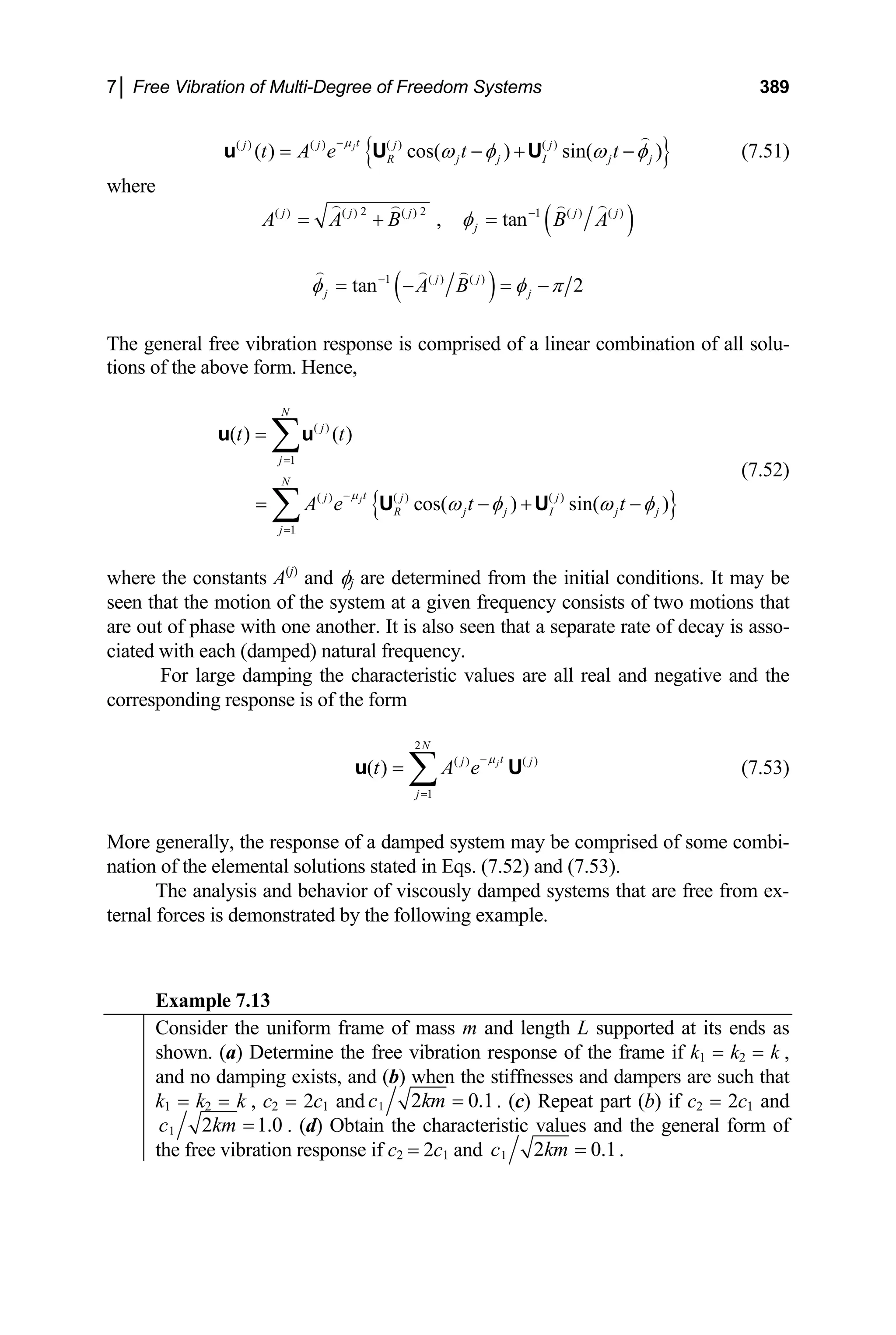
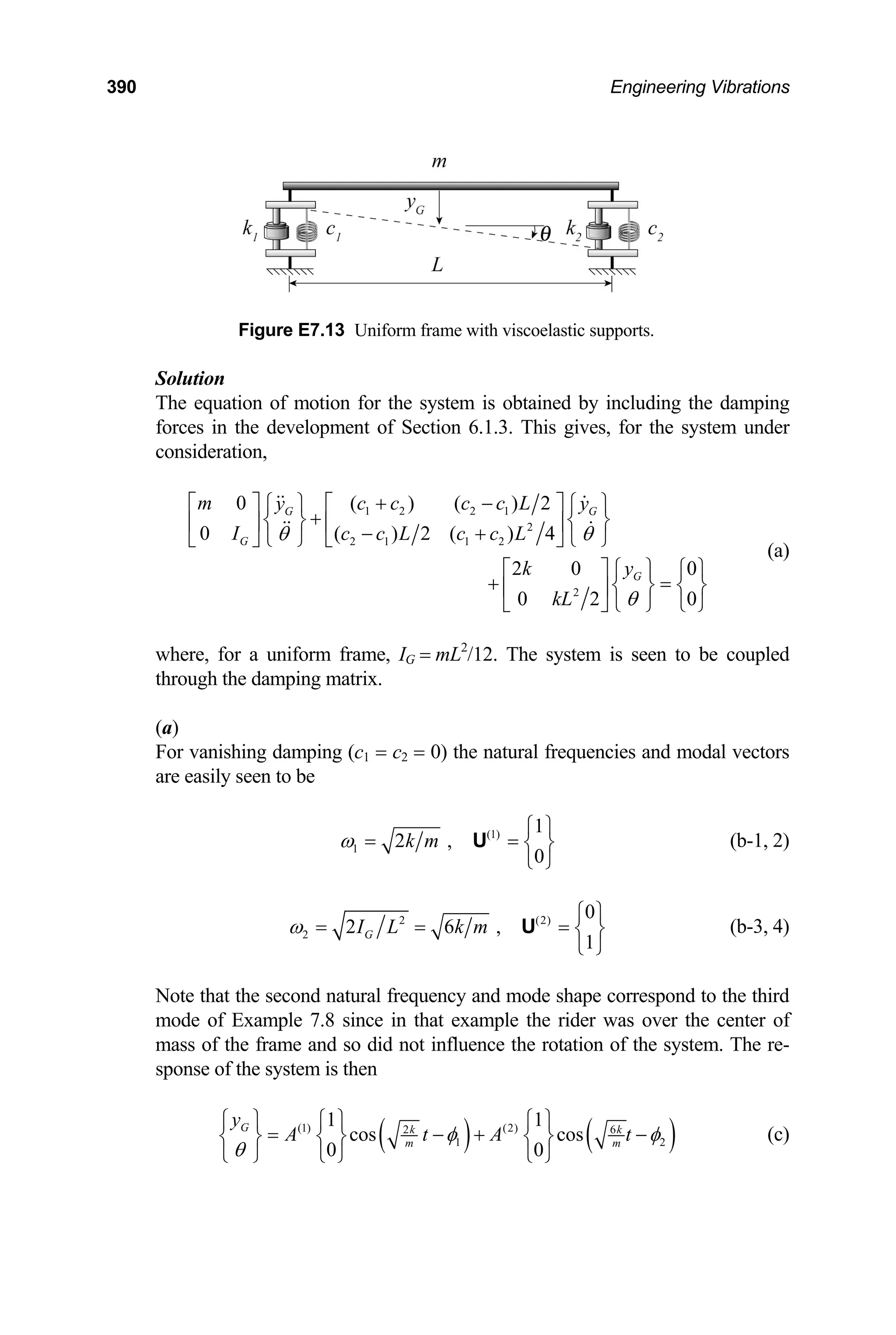
![7│ Free Vibration of Multi-Degree of Freedom Systems 391
(b)
The characteristic value problem for the damped system takes the form
{ }
{ }
2
1 2 2 1 1
2 2 2
2
2 1 1 2
( ) 2 ( ) 2 0
0
( ) 2 ( ) 4 2
G
m c c k c c L U
U
c c L I c c L kL
α α α
α α α
⎡ ⎤
+ + + − ⎧ ⎫ ⎧ ⎫
⎢ ⎥ =
⎨ ⎬ ⎨ ⎬
⎢ ⎥
− + + + ⎩ ⎭
⎩ ⎭
⎣ ⎦
(d)
Setting the determinant of the square matrix of Eq. (d) to zero (and dividing the
resulting equation by mIGω0
4
) gives the characteristic equation
[ ] [ ] [ ]
4 3 2
1 2 1 2 1 2
ˆ ˆ ˆ ˆ ˆ
( ) 4( ) 4(1 3 ) 6( ) 3 0
α α α η η α ηη α η η
= + + + + + + + =
F (e)
where
0
α̂ α ω
= (f)
0 2k m
ω = (g)
1 1 2 2
2 , 2
c mk c m
η η
= = k (h-1, 2)
For η2 = 2η1 and η1 = 0.1 we find, using the MATLAB solver “roots,” that
(i)
(1)
,
(2)
,
ˆ 0.1499 0.9964
ˆ 0.4501 1.6590
a b
a b
i
i
α
α
= − ±
= − ±
The first row of Eq. (d) gives, for 2 1
c c
≠ ,
( )
2 ( ) ( )
( )
( ) ( )
1 2 1
2 1
( )
2 1
( ) 2
2
( )
j j
j
j j
j
m c c k U
U P
L
c c
α α
α
+ + +
= − = − +
−
iQ U L (j)
where
2
( )
1 2
( )
2
( )
2 1
ˆ ˆ ˆ
( )
2
ˆ ( )
j
j
j
j
P
j
α µ η η µ
α η η
⎡ ⎤
− + + −
⎣
=
−
⎦ (k)
2
( )
( )
2
( )
2 1
ˆ ˆ
2 1
ˆ ( )
j
j
j
j
Q
ω α
α η η
⎡ ⎤
−
⎢ ⎥
⎣ ⎦
=
−
(l)
2
( ) 2 2
ˆ ˆ
j
ˆ
j j
α µ ω
= + (m)](https://image.slidesharecdn.com/engineeringvibrations-240713005818-b85f16c0/75/Engineering-Vibrations-Engineering-Vibrations-413-2048.jpg)
![396 Engineering Vibrations
ˆ ⎡ ⎤
= ⎢ ⎥
⎣ ⎦
I 0
I
0 I
is the identity matrix. The characteristic equation for the above eigenvalue
problem is then
2 2
N N
×
ˆ
det ( ) 0
α α
⎡ ⎤
− = =
⎣ ⎦
S I F (7.65)
which yields 2N roots, α = α1, α2, ... α2N. For each eigenvalue αj (j = 1, 2, …, 2N)
there is an associated eigenvector ( )
ˆ .
j
U More precisely, ( )
ˆ j
U is said to be the right
eigenvector of the nonsymmetric matrix S. The solution of Eq. (7.59) is then com-
prised of a linear combination of all such solutions. Hence,
2
( ) ( )
1
ˆ
( ) j
N
t
j j
j
t A e
α
=
= ∑
z U
j
U
(7.66)
It follows from Eqs. (7.60), (7.63) and (7.66) that
(7.67)
2
( ) ( )
1
( ) j
N
t
j
j
t A e
α
=
= ∑
u
The response corresponding to complex roots with negative real parts or to negative
real roots follows directly from the development of the preceding section beginning
with Eqs. (7.46) and (7.47), and leading to Eqs. (7.52) and (7.53). It is pertinent to
note that the eigenvalues, αj (j = 1, 2, …, 2N), and the associated subeigenvectors,
U(j)
, of S correspond directly with the roots and vectors of the solution described in
Section 7.4.1. This may be seen by utilizing the identity
11 12 1
11 22 21 11 12
21 22
−
= −
A A
A A A A A
A A
(7.68)
for the determinant of a partitioned matrix in Eq. (7.65) and noting that
[ ] 1 1
.
α α
− −
=
I I Doing this results in a characteristic equation that is identical to Eq.
(7.45). The roots of Eq. (7.45) therefore correspond to the eigenvalues of S. It follows
that the vector comprised of the first N rows of the eigenvector of the system matrix
S, the subvector U appearing in Eq. (7.63), corresponds to the characteristic vector U
of Eq. (7.44) for the same value of α. The various forms of Eq. (7.67) for complex
and real eigenvalues therefore correspond directly to the forms derived in the previ-
ous section by way of direct solution of the equation of motion, Eq. (7.42).](https://image.slidesharecdn.com/engineeringvibrations-240713005818-b85f16c0/75/Engineering-Vibrations-Engineering-Vibrations-418-2048.jpg)
![398 Engineering Vibrations
1
2
1
1 2 2 1
2
2 1 1 2
ˆ 0 1 0
ˆ
0 0 1
ˆ
1 0 ( ) ( ) 2 0
ˆ
0 3 6( ) 3( ) 0
U
U
V
V
α
α
η η α η η
η η η η α
−
⎡ ⎤ ⎧ ⎫ 0
0
⎧ ⎫
⎢ ⎥ ⎪ ⎪ ⎪ ⎪
− ⎪ ⎪ ⎪ ⎪
⎢ ⎥ =
⎨ ⎬ ⎨ ⎬
⎢ ⎥
− − + + − − ⎪ ⎪ ⎪ ⎪
⎢ ⎥ ⎪ ⎪ ⎪ ⎪
− − − − + − ⎩ ⎭
⎩ ⎭
⎣ ⎦
(f)
We next require that the determinant of the square matrix of Eq. (f) vanishes.
This results in the characteristic equation
[ ] [ ] [ ]
4 3 2
1 2 1 2 1 2
ˆ ˆ ˆ ˆ ˆ
( ) 4( ) 4(1 3 ) 6( ) 3 0
α α α η η α ηη α η η
= + + + + + + + =
F (g)
which is seen to be identical to the characteristic equation of Example 7.13, as
it should be. The roots of the characteristic equation, for η2 = 1.0 and η1 = 0.5,
are then
ˆ 0.6129, 4.0251, 0.6810 0.8673
α = − − − ± (h)
Substituting the first row of Eq. (f) into the third row and solving the resulting
expression for U2 in terms of U1 gives, for each respective characteristic value,
(i)
(1) (2) (3,4)
1 1 1
, ,
2.98 11.1 1.04 0.616i
⎧ ⎫ ⎧ ⎫ ⎧
= = =
⎨ ⎬ ⎨ ⎬ ⎨
−
⎩ ⎭ ⎩ ⎭ ⎩ ∓
U U U
⎫
⎬
⎭
The response of the system is then
0 0
0
0.613 4.03
(1) (2)
0.681
(3)
0 3 0 3
1 1
2.98 11.1
1 0
cos(0.867 ) sin(0.867 )
1.04 0.616
G t t
t
y L
A e A e
A e t t
ω ω
ω
θ
ω φ ω
− −
−
⎧ ⎫ ⎧ ⎫ ⎧ ⎫
= +
⎨ ⎬ ⎨ ⎬ ⎨ ⎬
⎩ ⎭ ⎩ ⎭ ⎩ ⎭
⎡ ⎤
⎧ ⎫ ⎧ ⎫
+ − +
⎢⎨ ⎬ ⎨ ⎬ ⎥
− −
⎩ ⎭ ⎩ ⎭
⎣ ⎦
φ
−
(j)
Orthogonality
The (right) eigenvectors (j = 1, 2, …, 2N) of the system matrix S are not, in gen-
eral, mutually orthogonal in the conventional sense. However, a broader view of the
problem reveals an orthogonality relation between the right eigenvectors and the cor-
responding members of a related set of vectors, the left eigenvectors of S. We estab-
lish this relation in the following development. Toward this end, let us consider the
eigenvalue problem
( )
ˆ j
U](https://image.slidesharecdn.com/engineeringvibrations-240713005818-b85f16c0/75/Engineering-Vibrations-Engineering-Vibrations-420-2048.jpg)
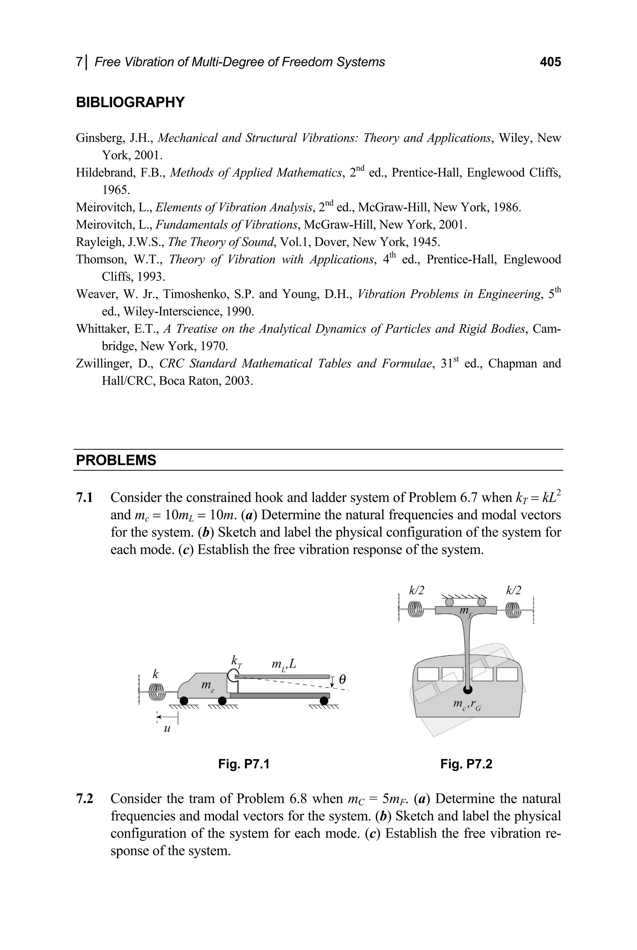
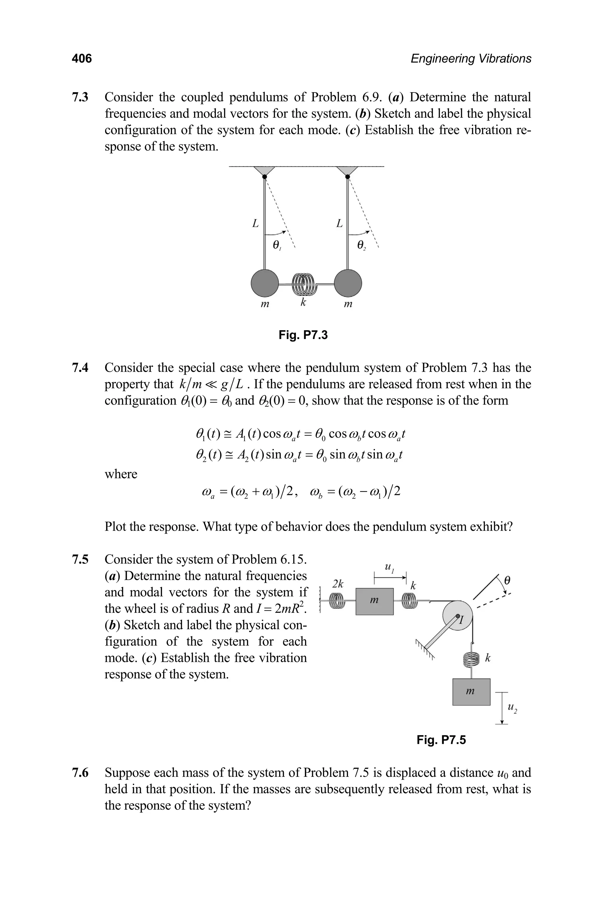
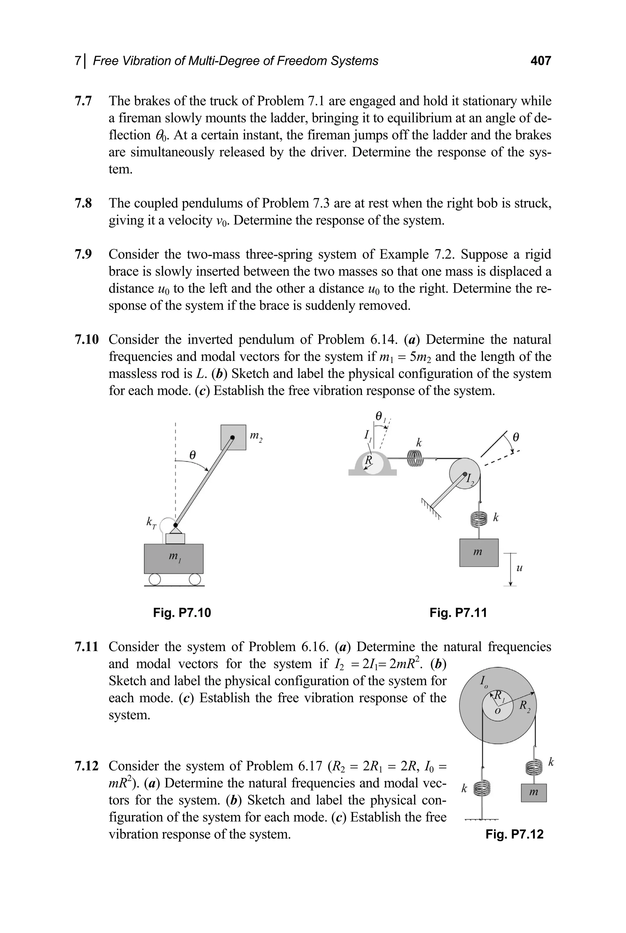
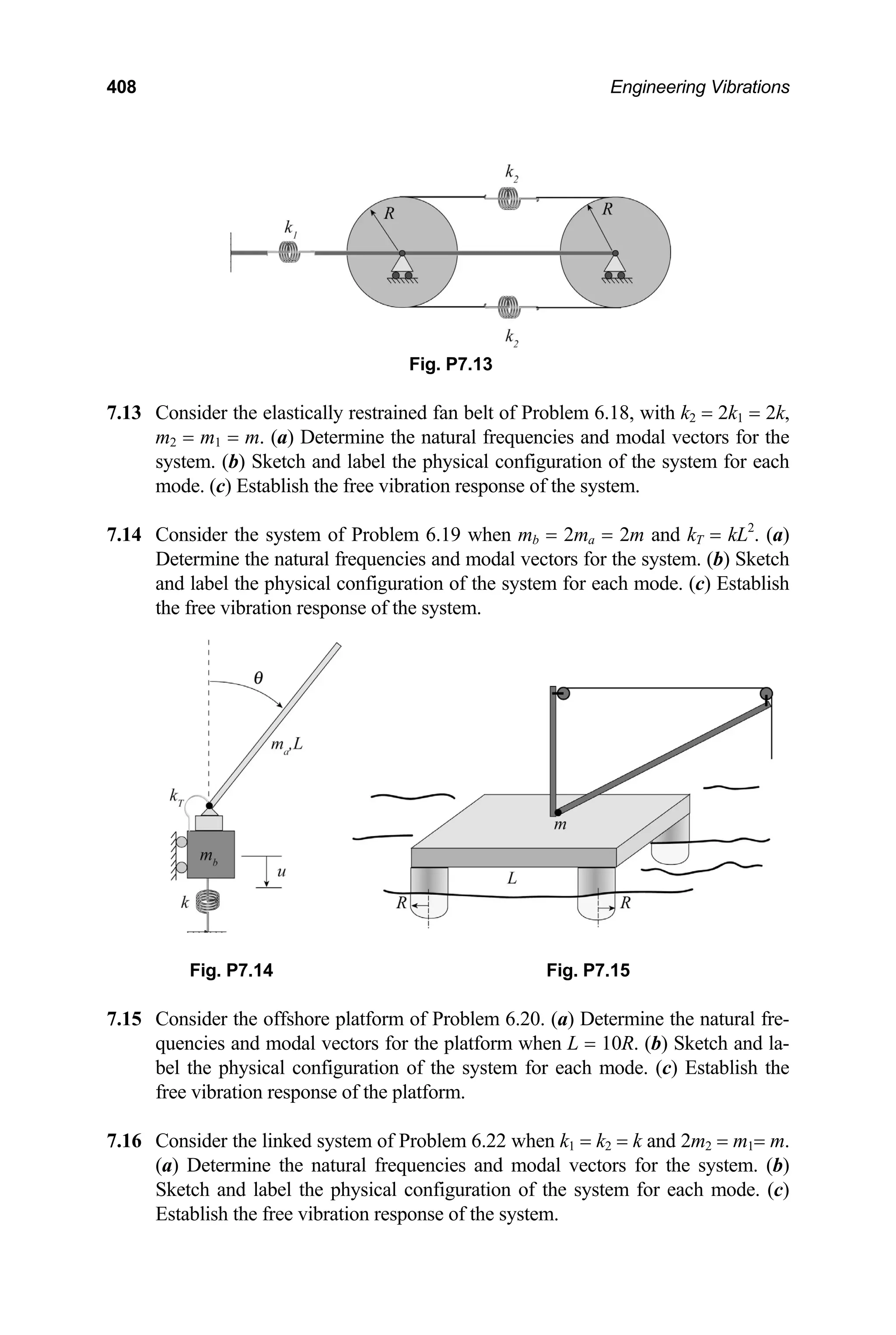
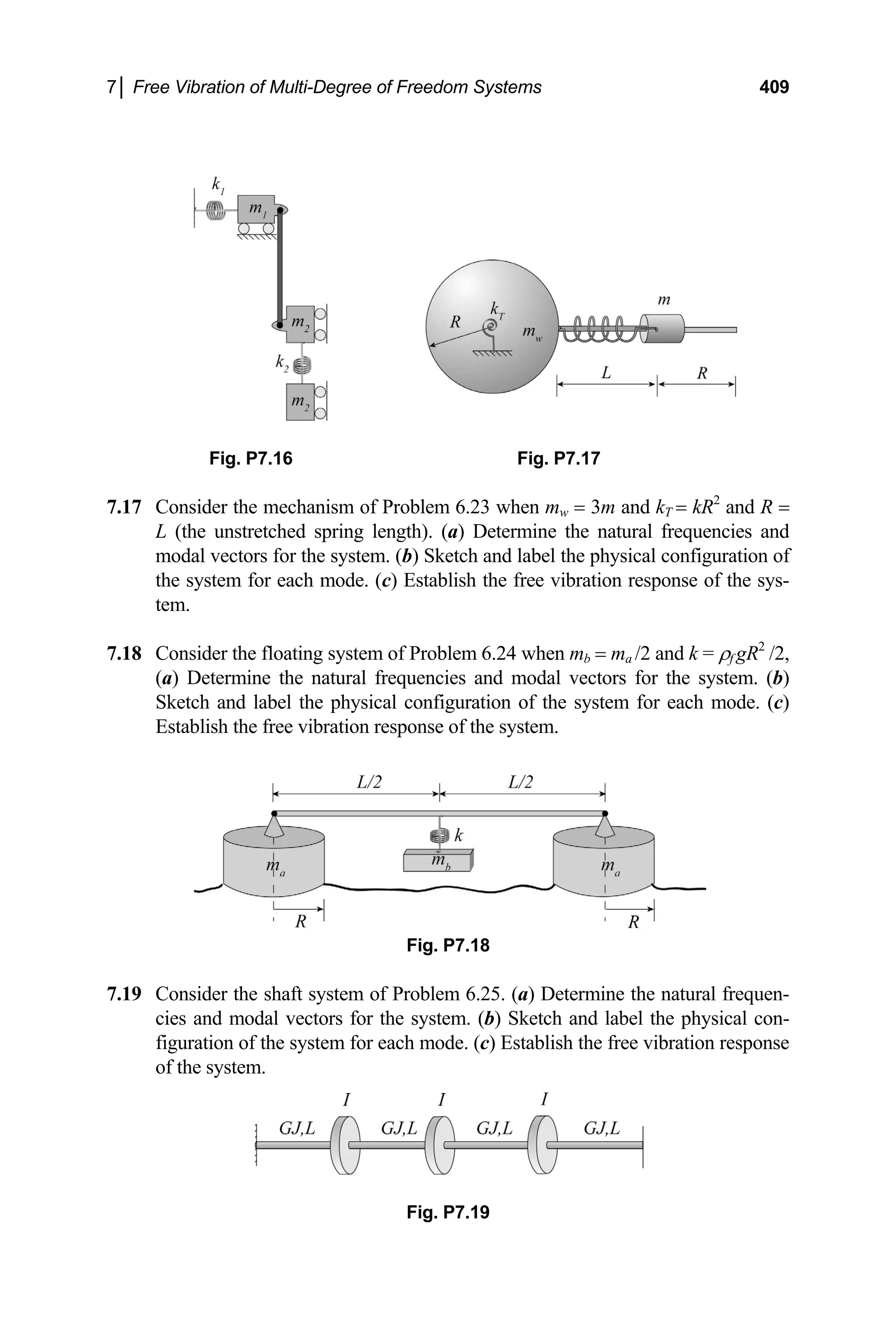
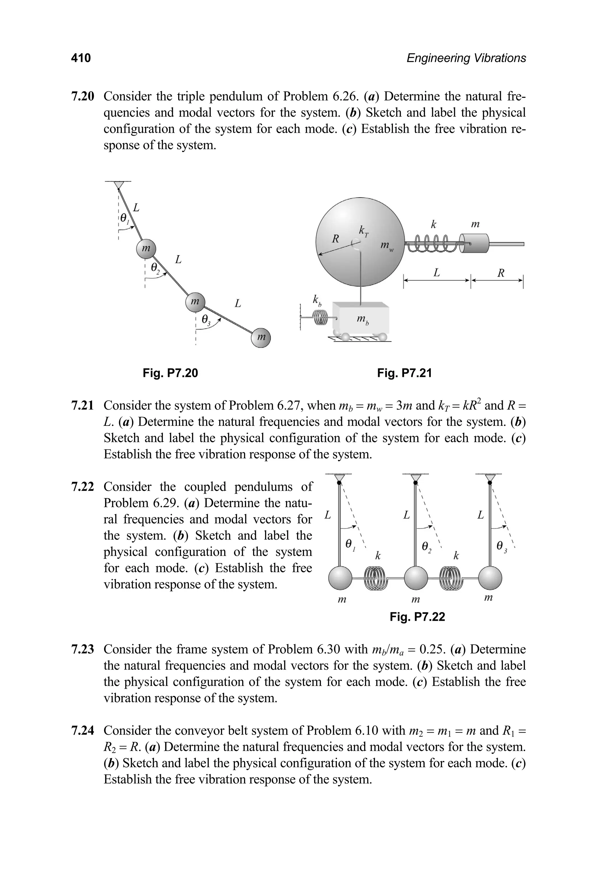
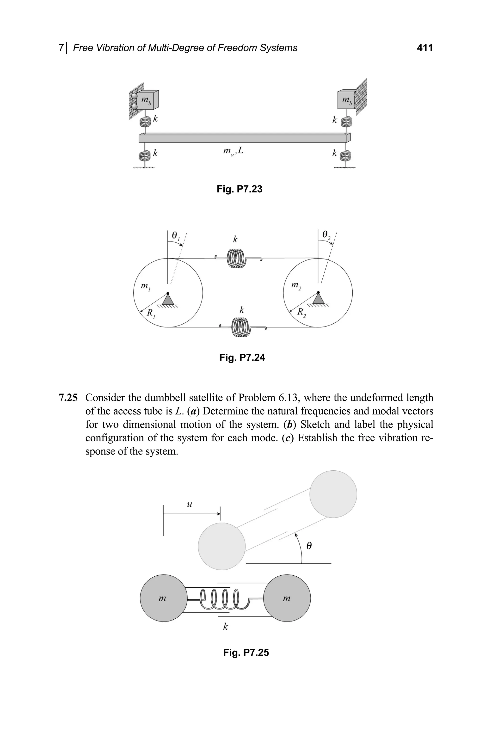
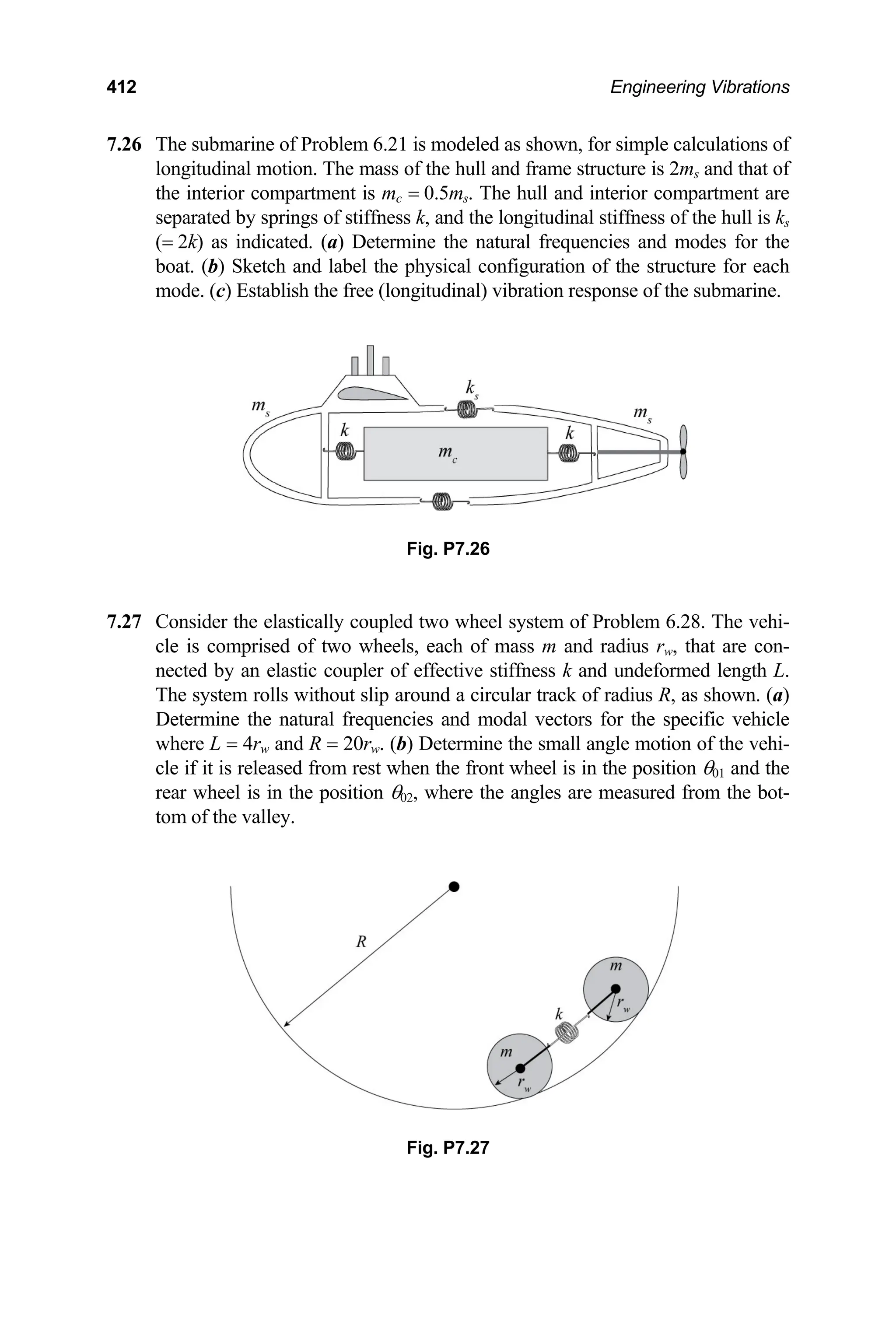
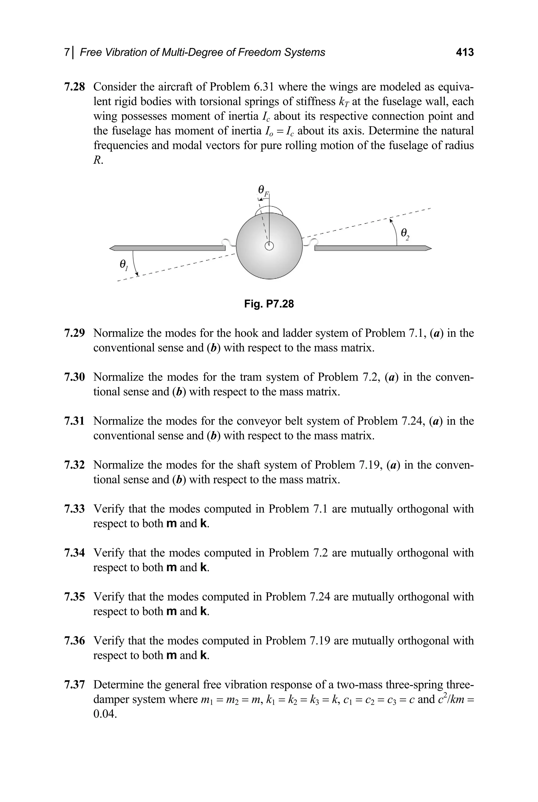
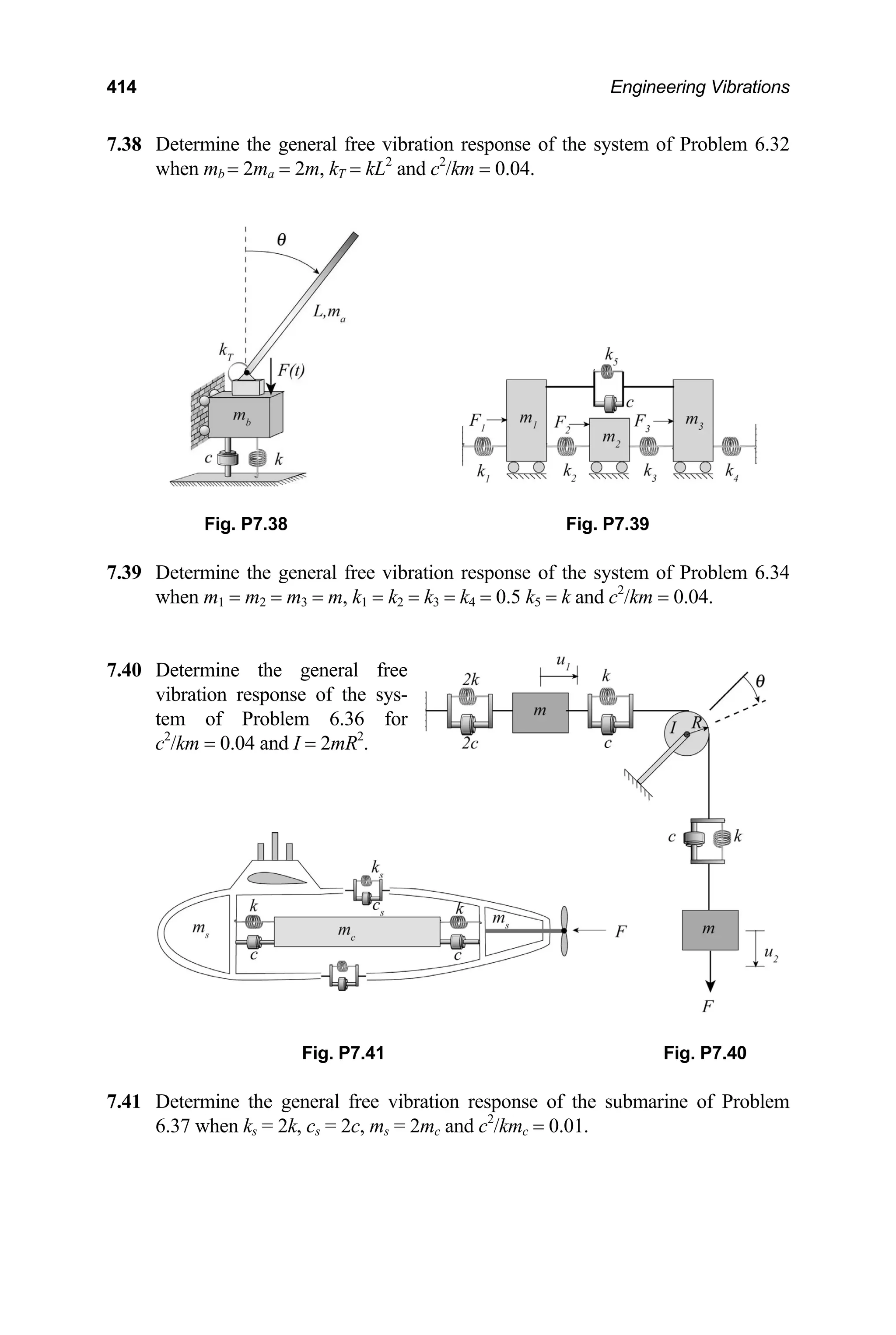
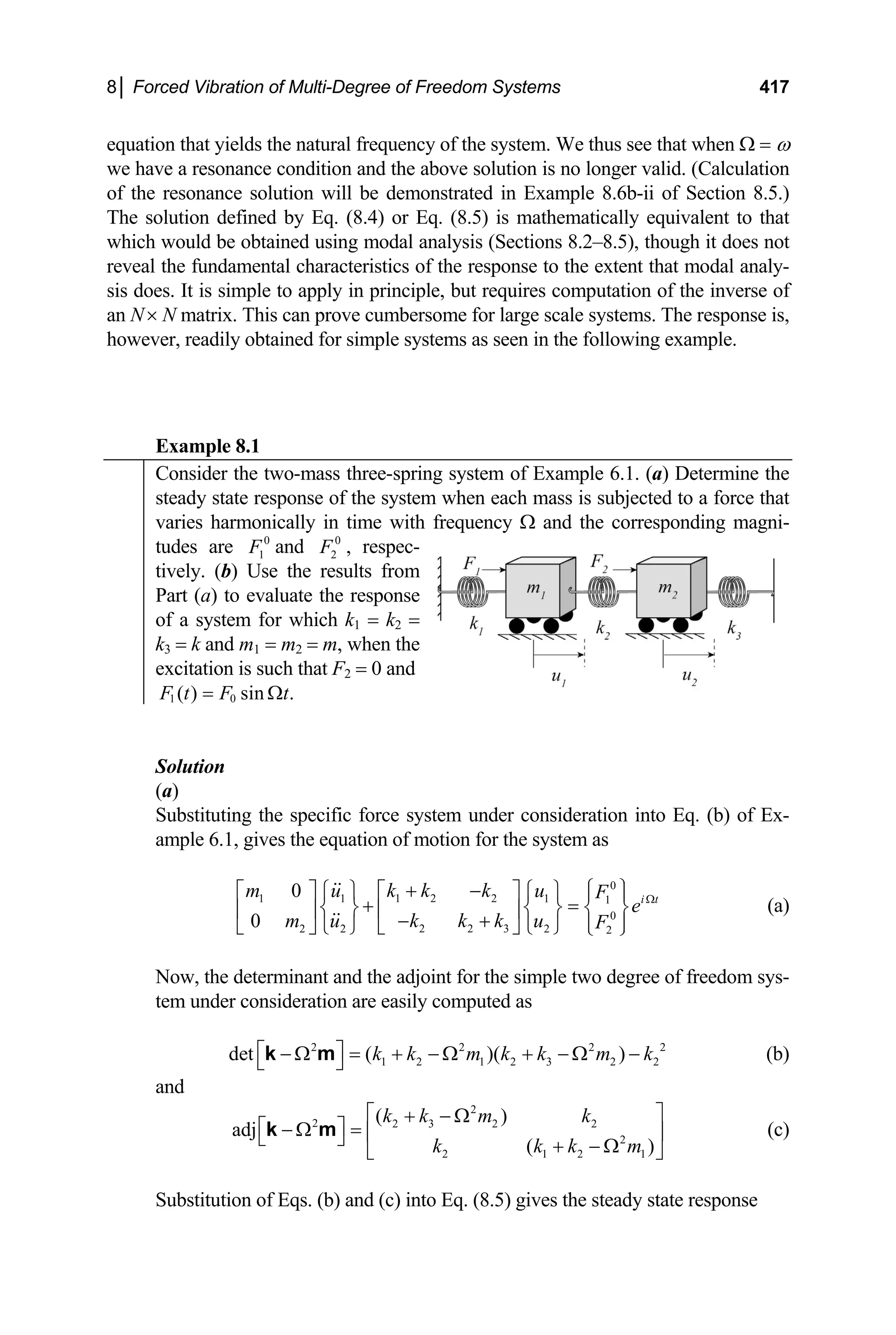
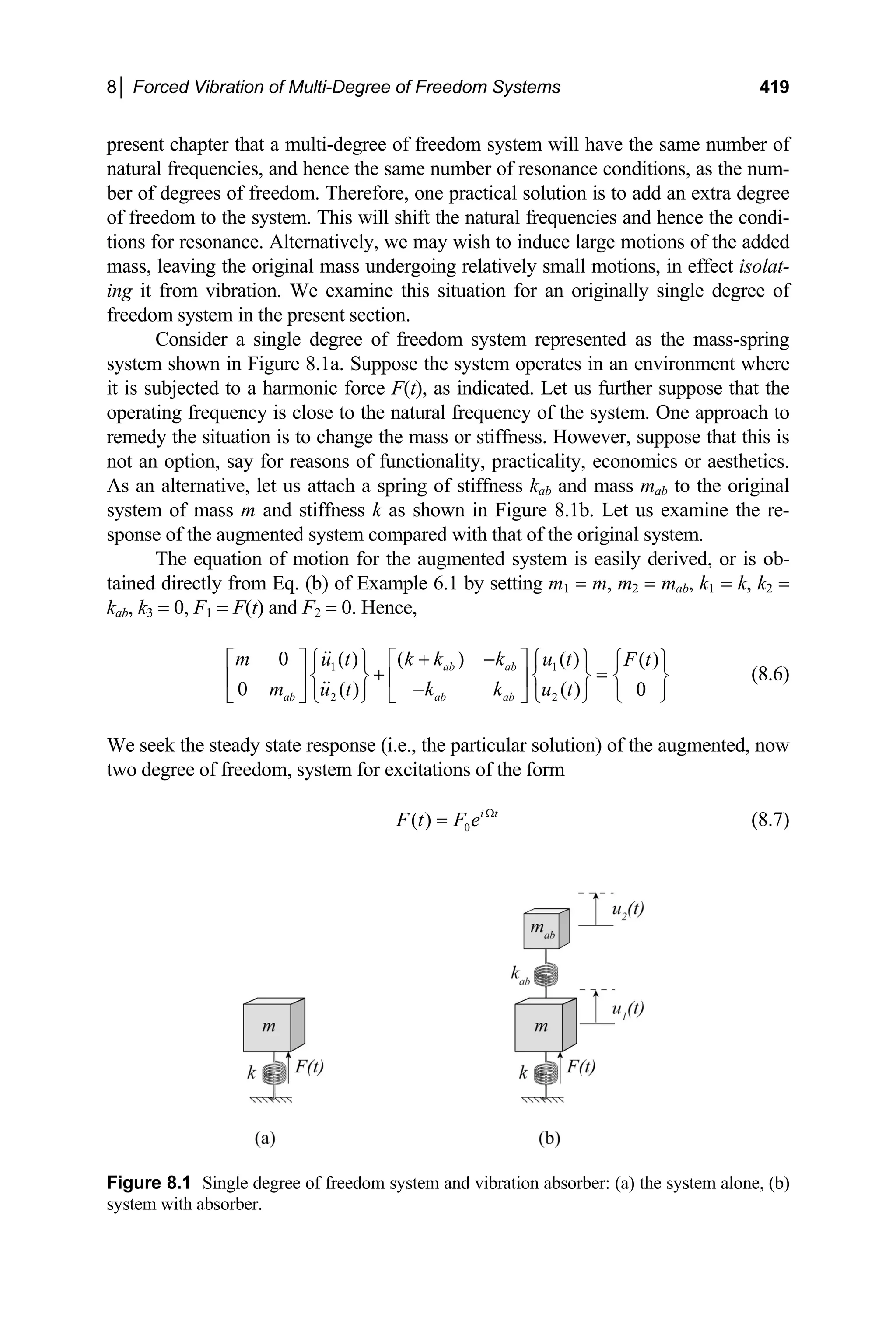

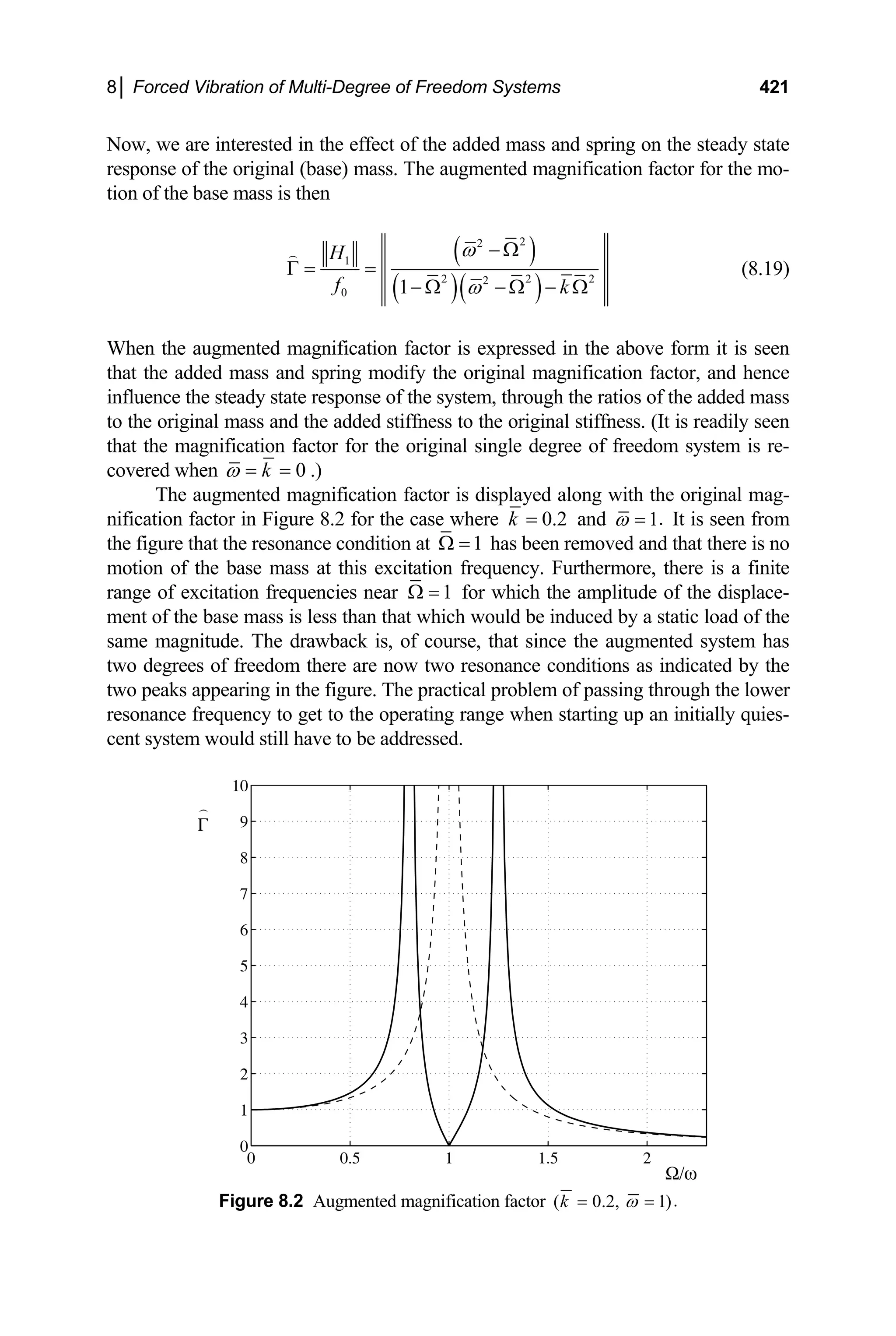
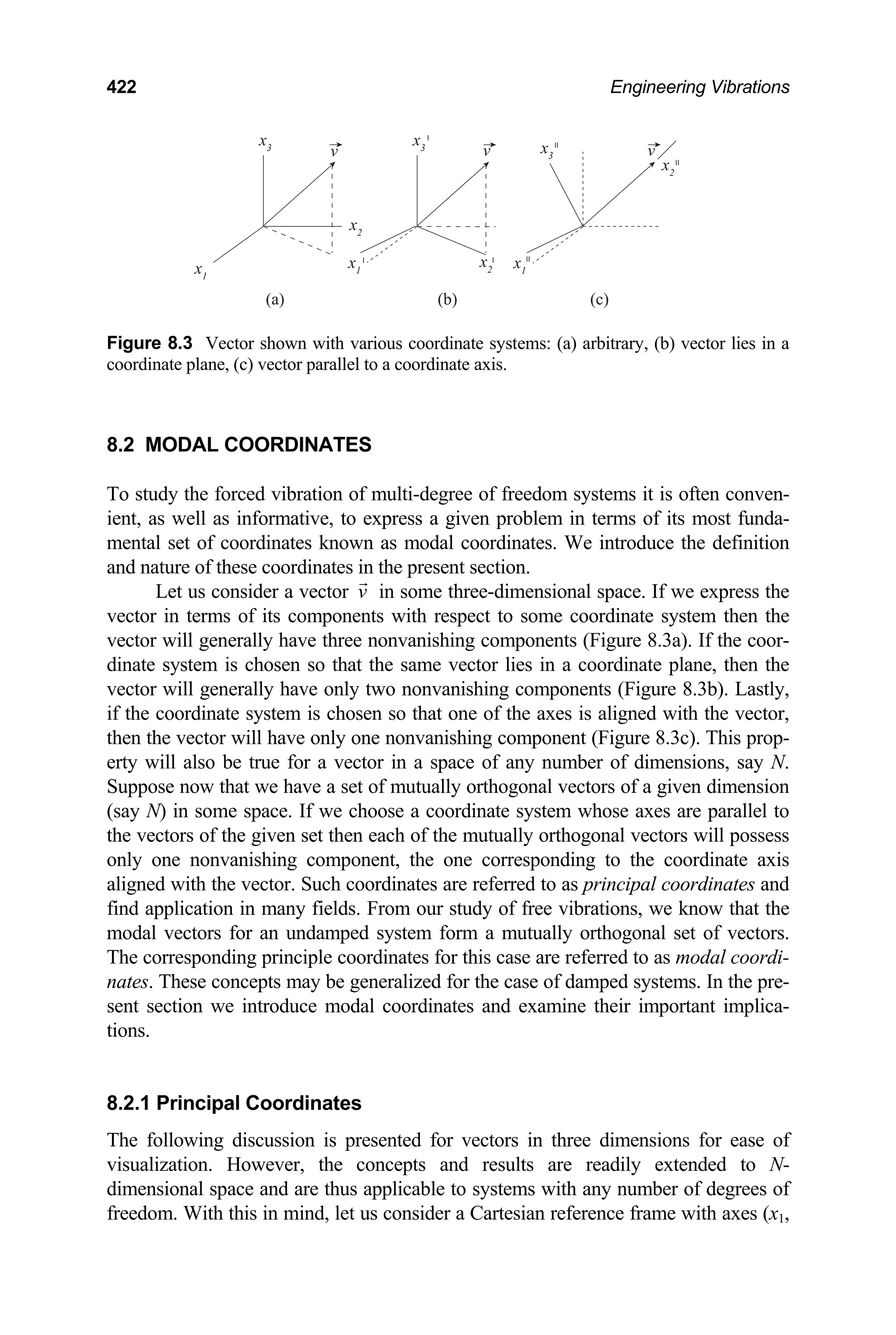
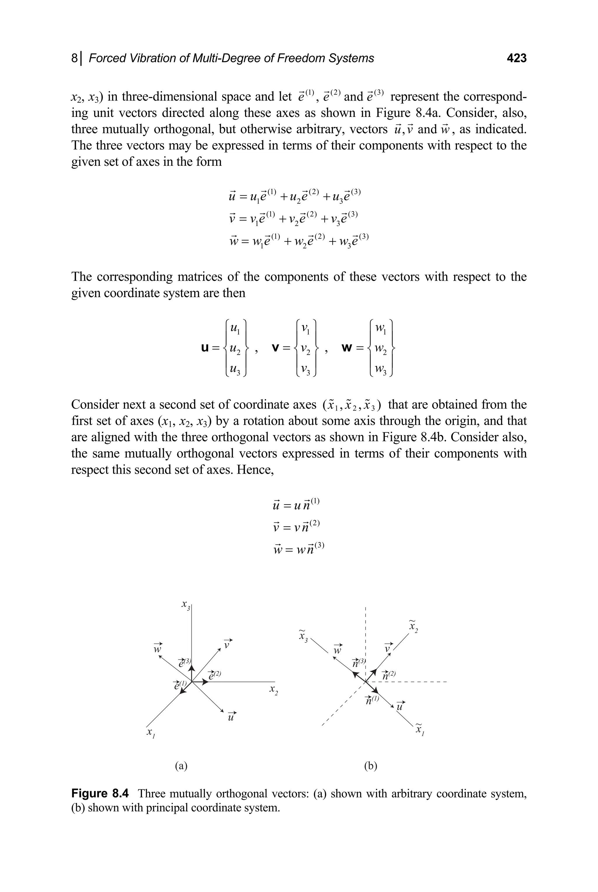
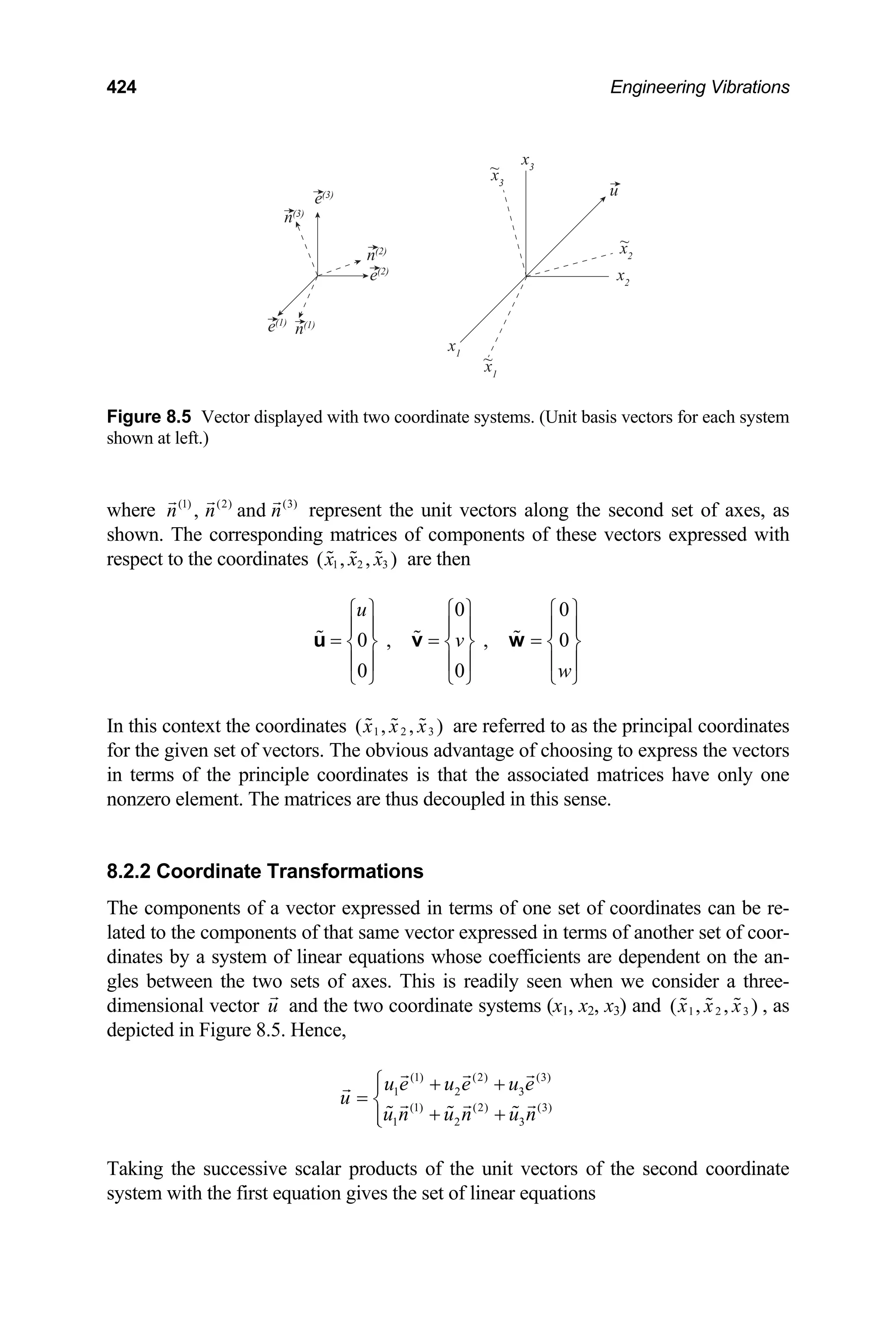
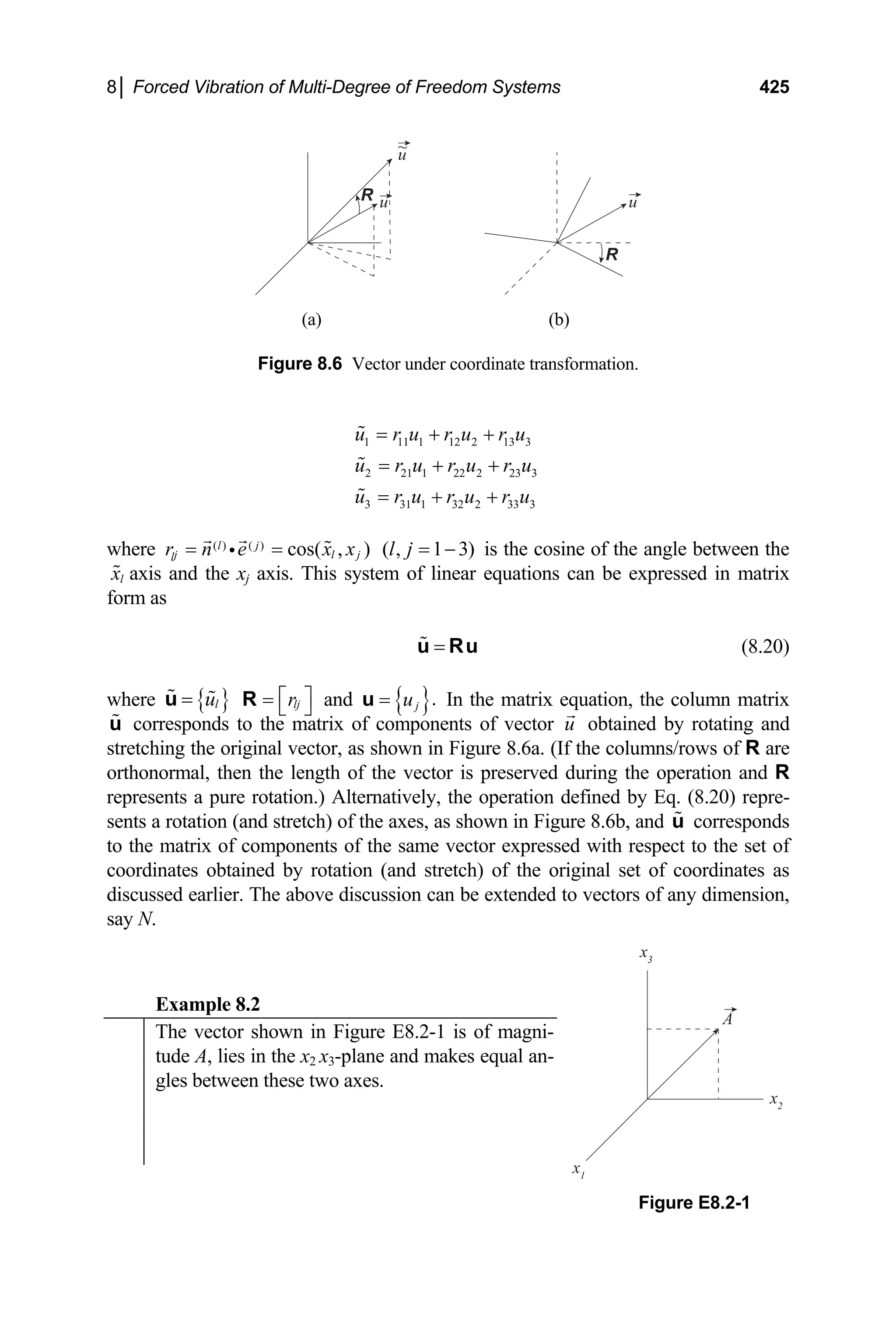
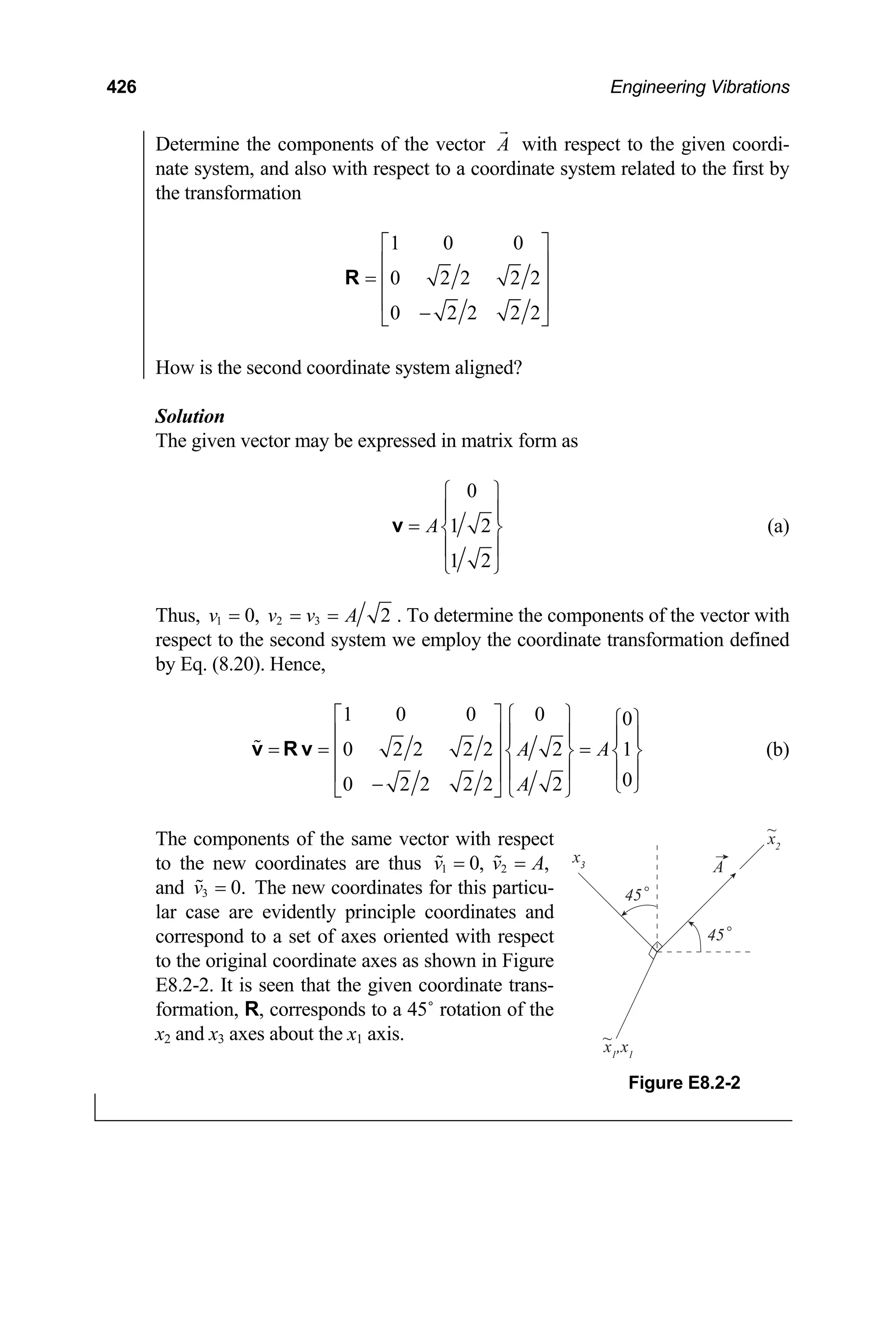
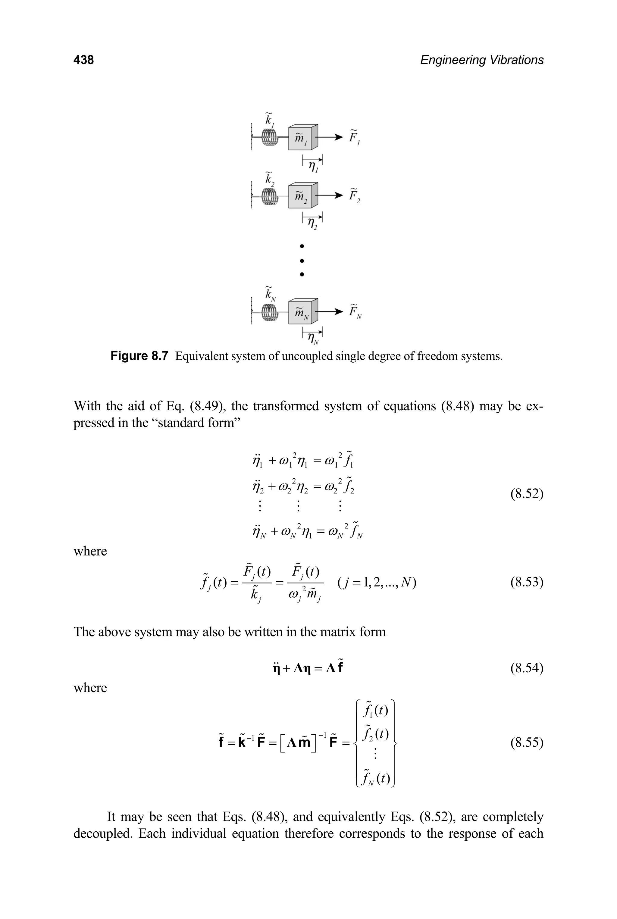
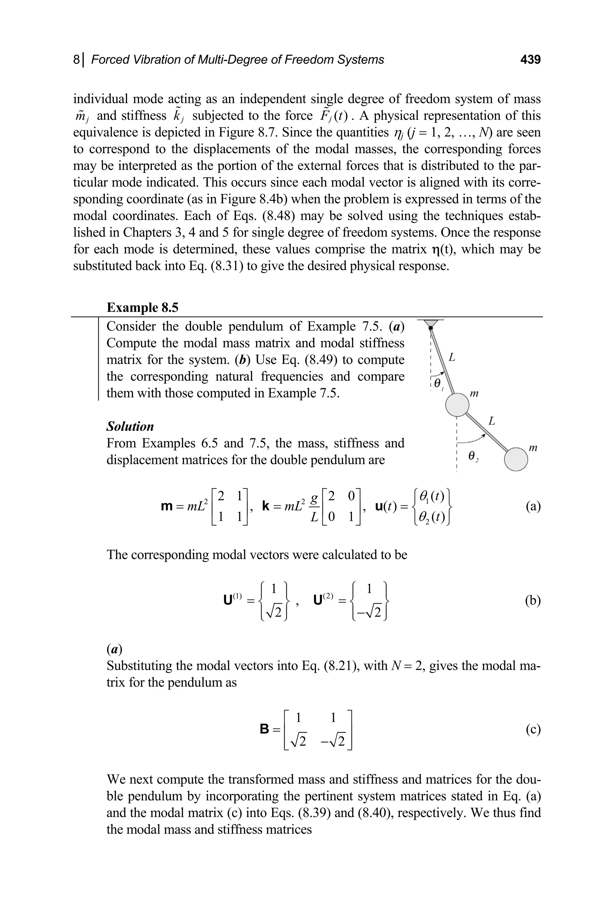
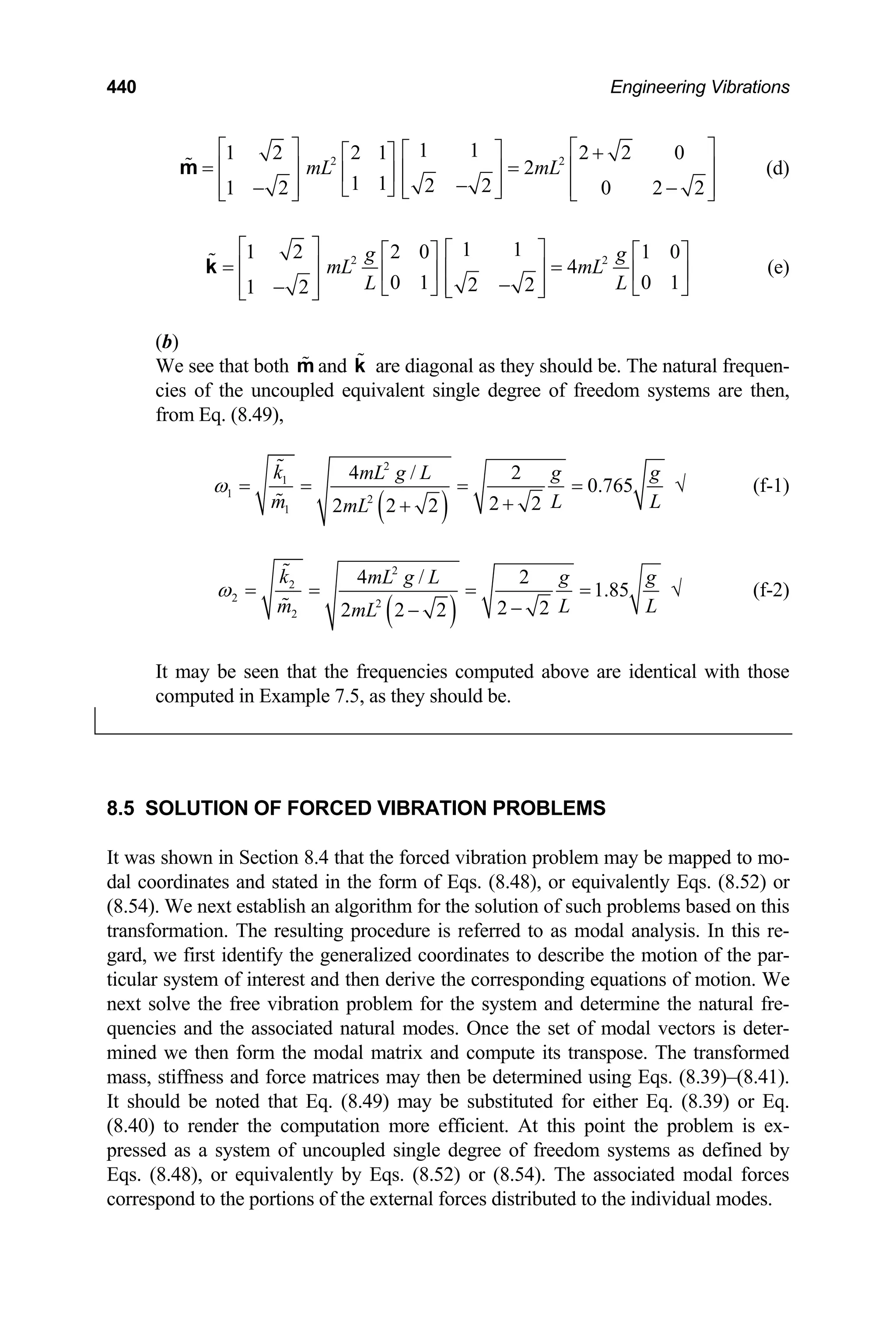
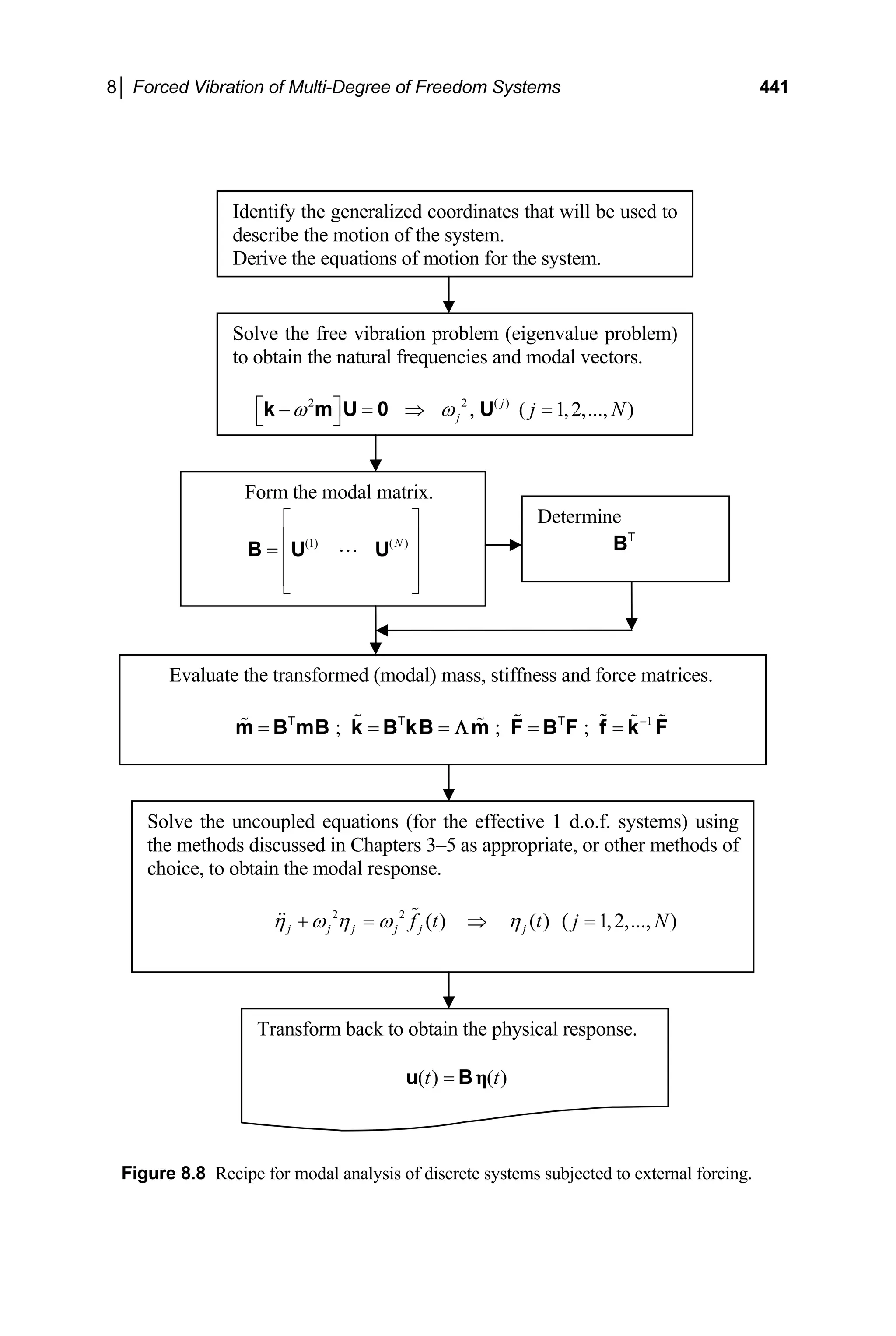
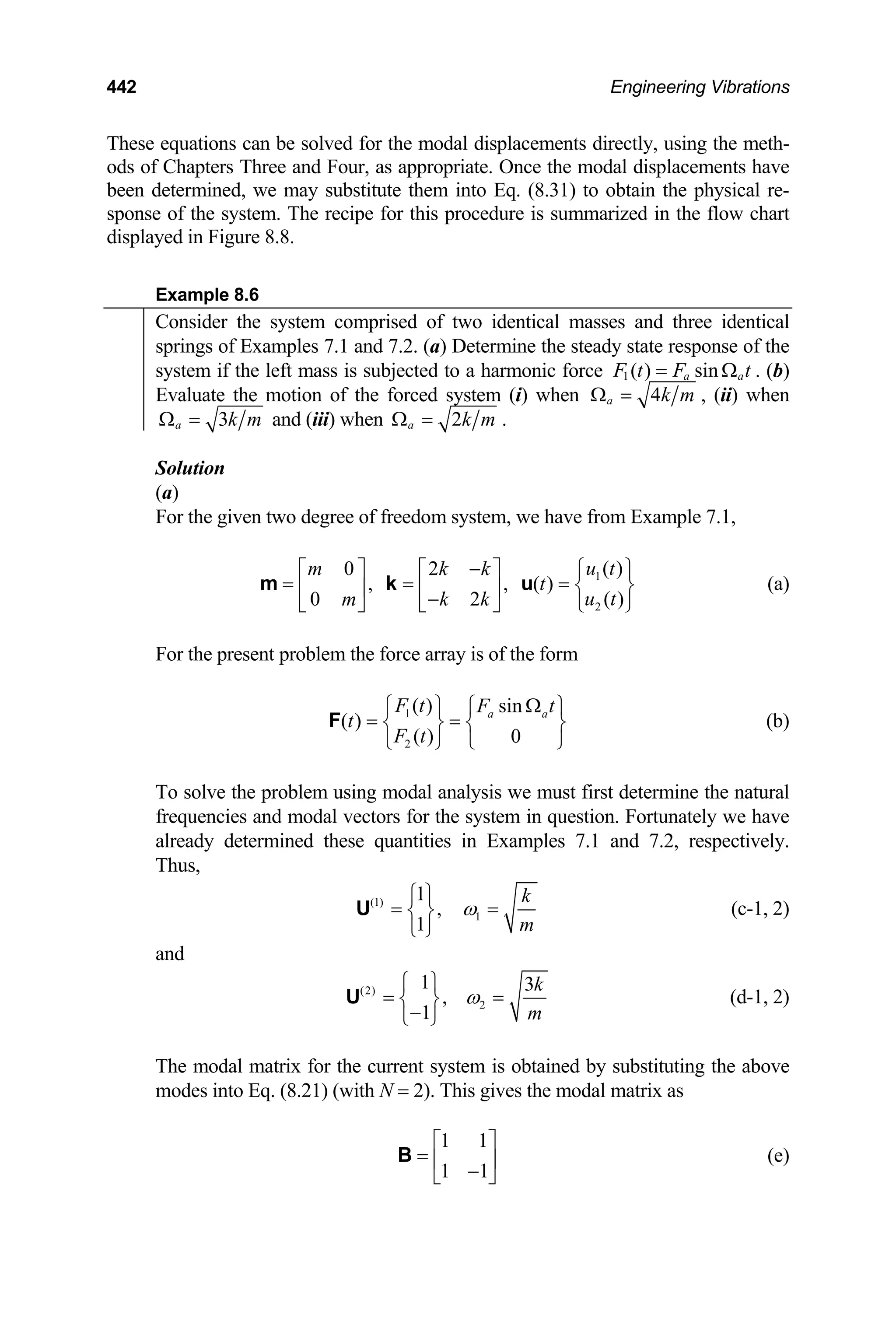
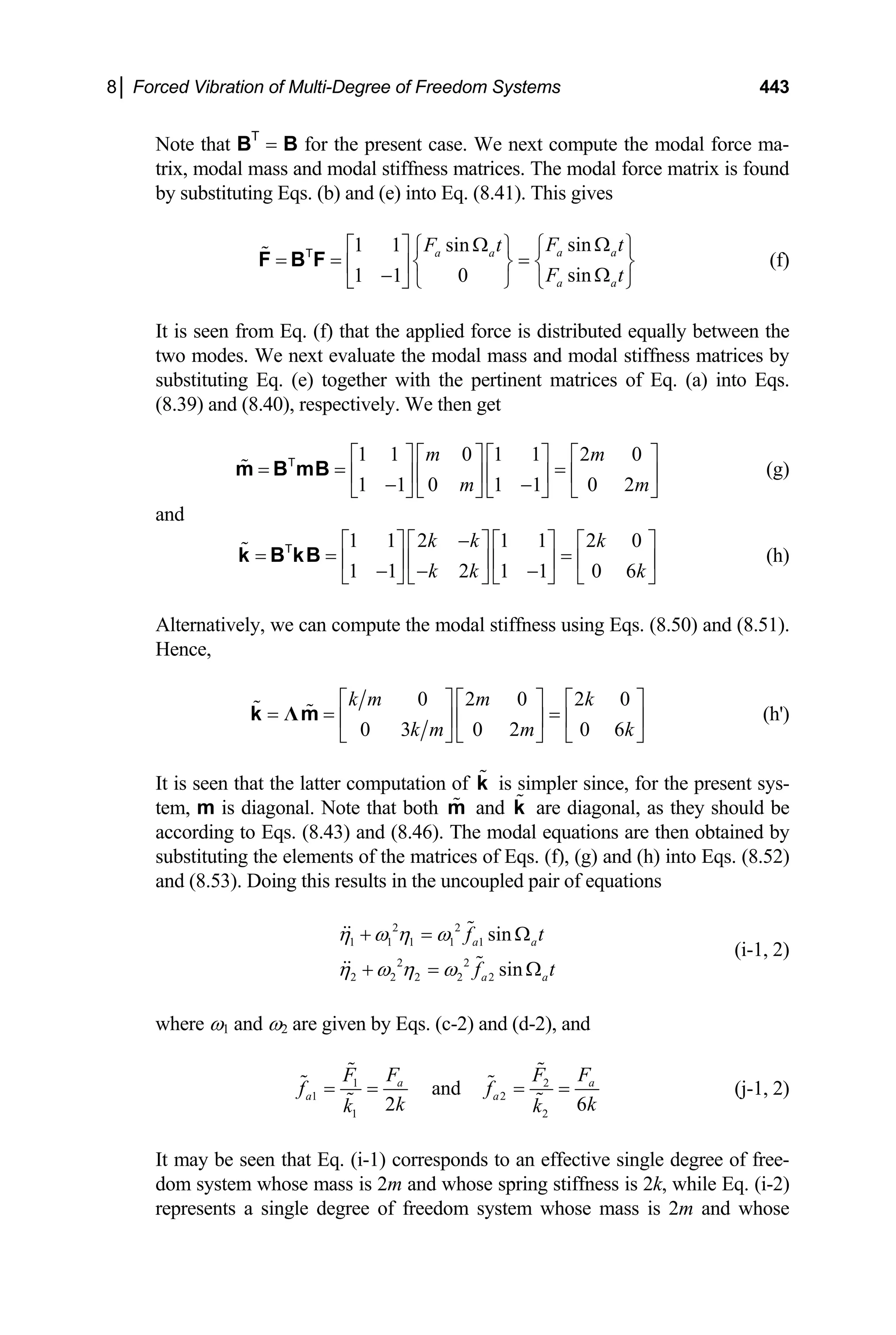
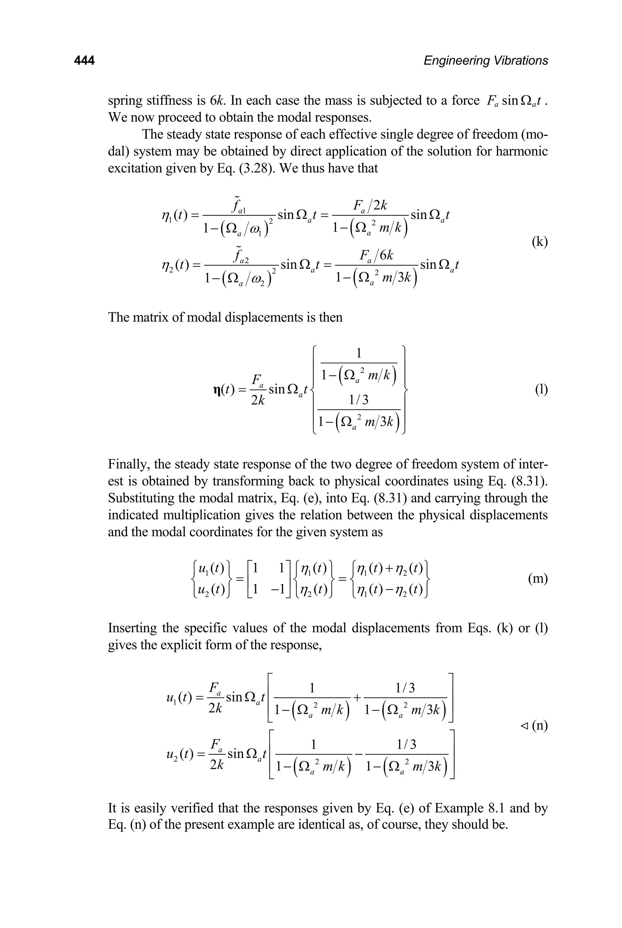
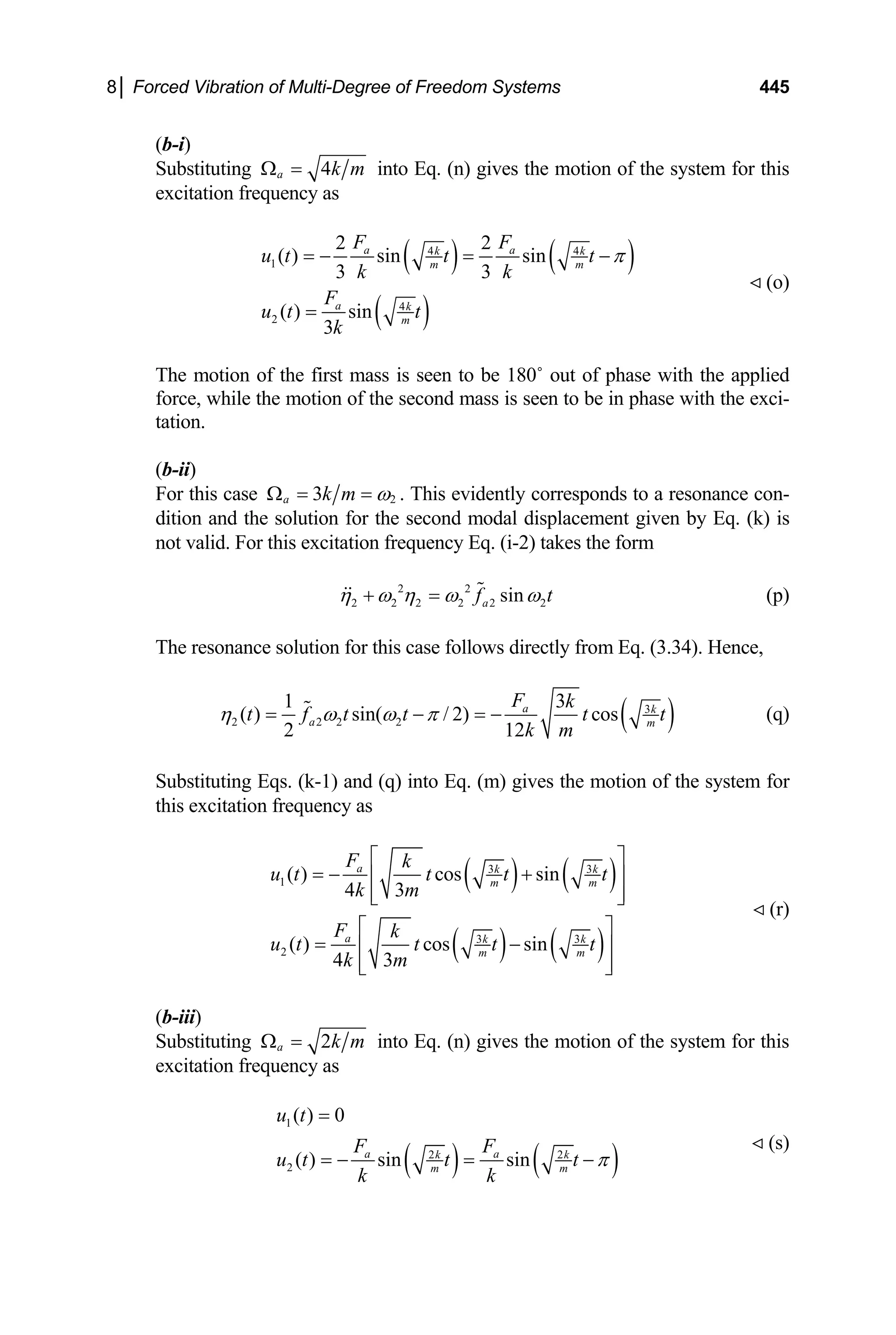
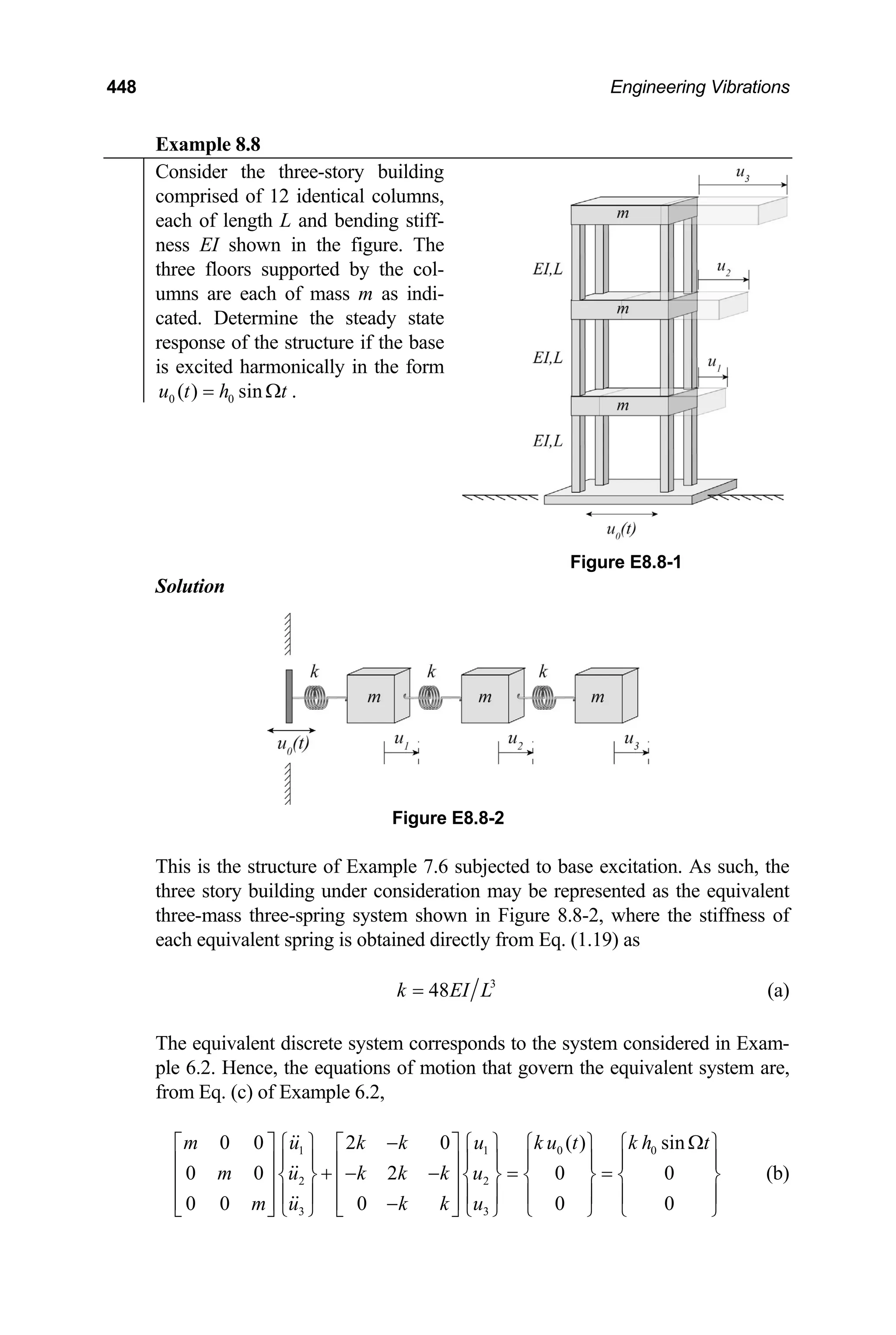
![450 Engineering Vibrations
The modal force matrix is easily computed as
0
0.328
sin 0.737
0.591
kh t
⎧ ⎫
⎪ ⎪
= = Ω ⎨ ⎬
⎪ ⎪
⎩ ⎭
F B F
T
(j)
Having computed the modal mass, modal stiffness and modal force matrices,
the modal equations for the three-story building are then
1 0.198 0.328 sin
m k k h0 t
η η
+ = Ω
t
(k-1)
2 2 0
1.56 0.737 sin
m k k h
η η
+ = Ω
t
(k-2)
3 3 0
3.25 0.591 sin
m k k h
η η
+ = Ω (k-3)
or, in standard form,
2 2 (1) (1) 0
1 1 1 1 0 0
0.328
sin ; 1.66
0.198
k h
f t f
k
η ω η ω
+ = Ω = = 0
h (l-1)
2 2 (2) (2) 0
2 2 2 2 0 0
0.737
sin ; 0.472
1.56
k h
f t f
k
η ω η ω
+ = Ω = = 0
h (l-2)
2 2 (1) (3) 0
3 3 3 3 0 0
0.591
sin ; 0.182
3.25
k h
f t f
k
η ω η ω
+ = Ω = = 0
h (l-3)
The steady state response for each mode [i.e., the solutions to Eqs. (l-1)–(l-
3)] can be written directly from Eq. (3.28). Hence, letting j j
ω
Ω ≡ Ω (j = 1,
2, 3), we obtain
( )
(1)
0 0
1 2 2 2
1 0
1.66
( ) sin sin
1 1 0.105
f h
t t
η
ω
= Ω =
− Ω − Ω
t
Ω (m-1)
( )
(2)
0 0
2 2 2 2
2 0
0.472
( ) sin sin
1 1 0.0134
f h
t t
η
ω
= Ω =
− Ω − Ω
t
Ω (m-2)
( )
(3)
0 0
3 2 2 2
3 0
0.182
( ) sin sin
1 1 0.00640
f h
t t
η
ω
= Ω =
− Ω − Ω
t
Ω (m-3)
Finally, the response of the structure is obtained by transforming back to physi-
cal coordinates using Eq. (8.30). Hence,](https://image.slidesharecdn.com/engineeringvibrations-240713005818-b85f16c0/75/Engineering-Vibrations-Engineering-Vibrations-472-2048.jpg)
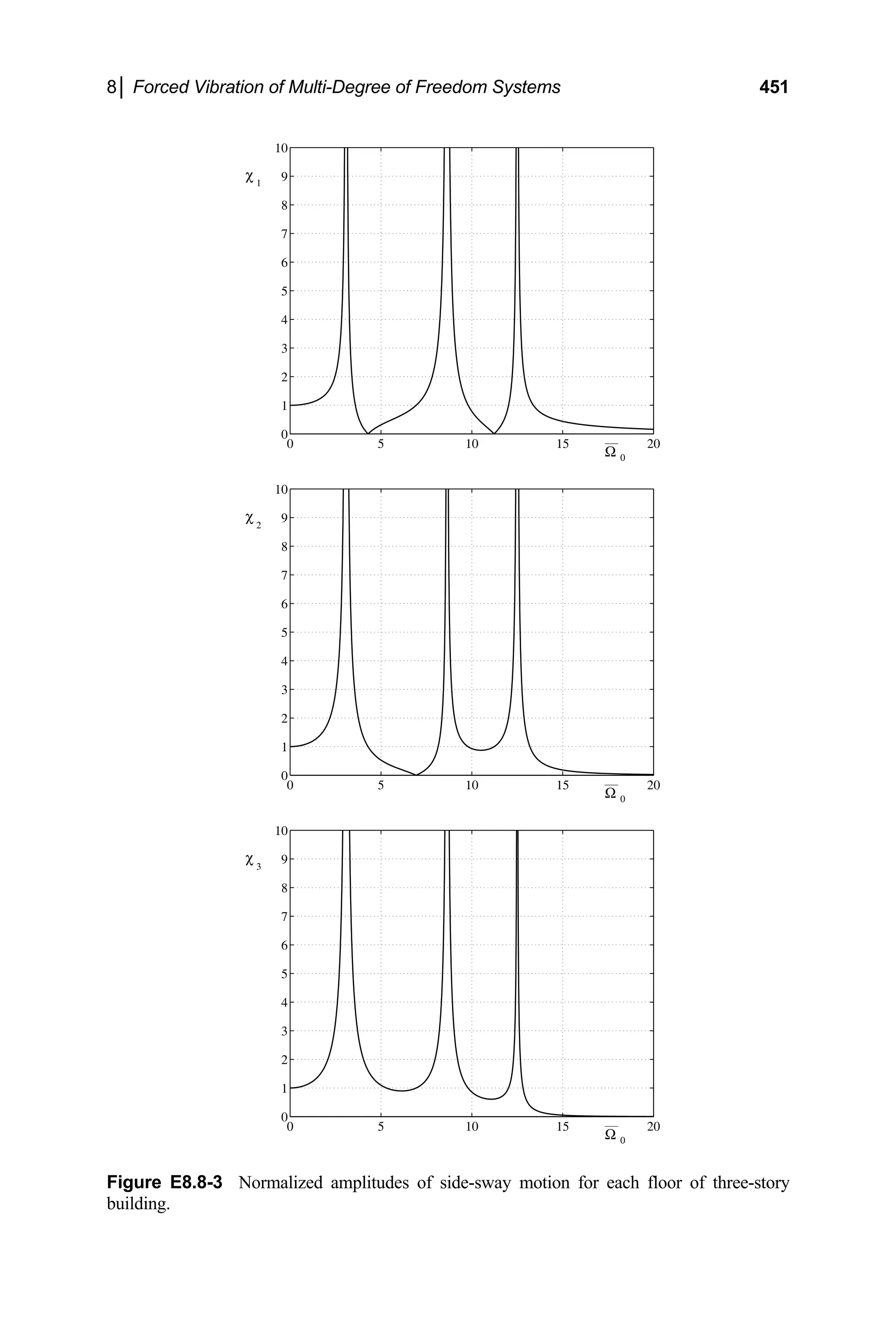
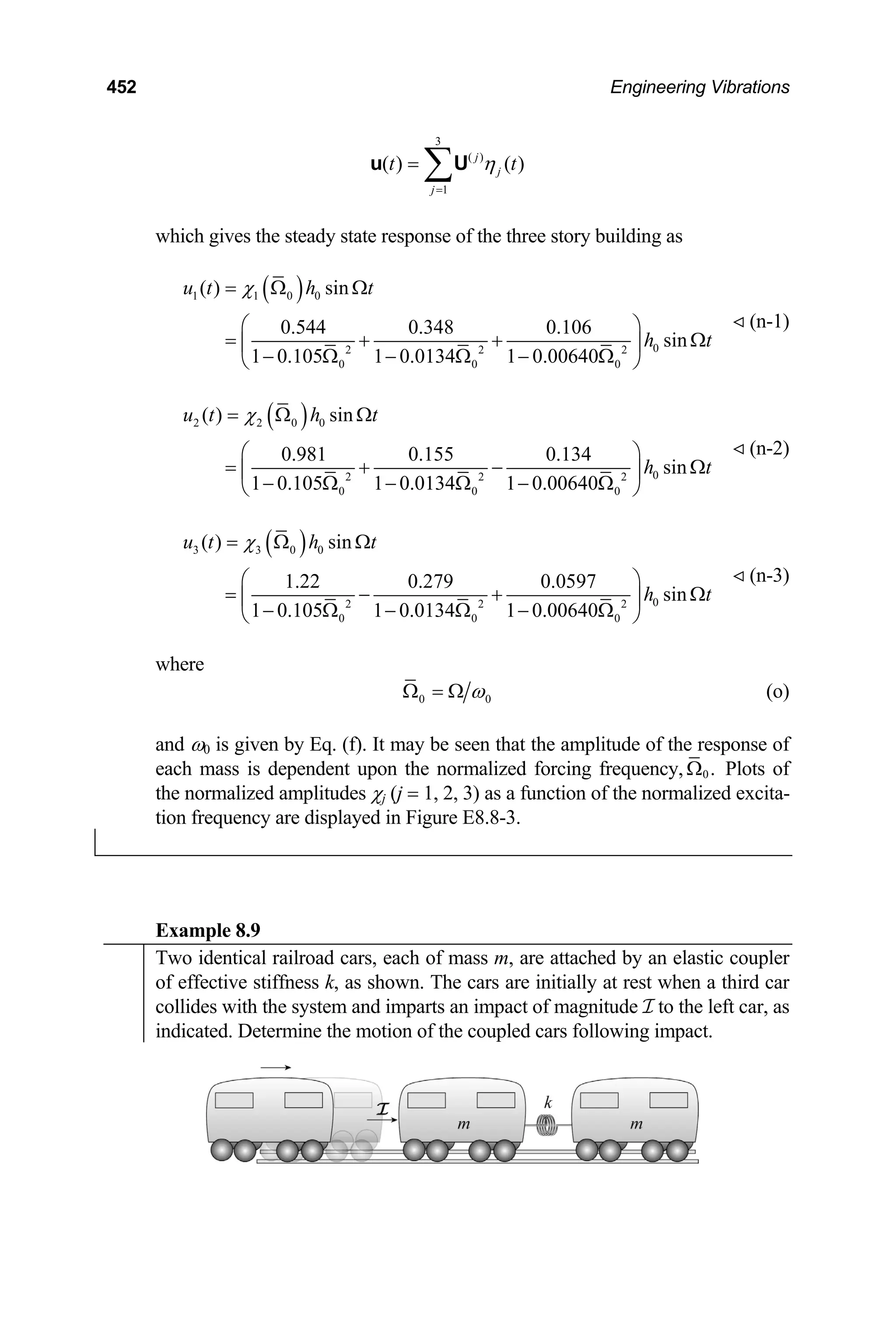
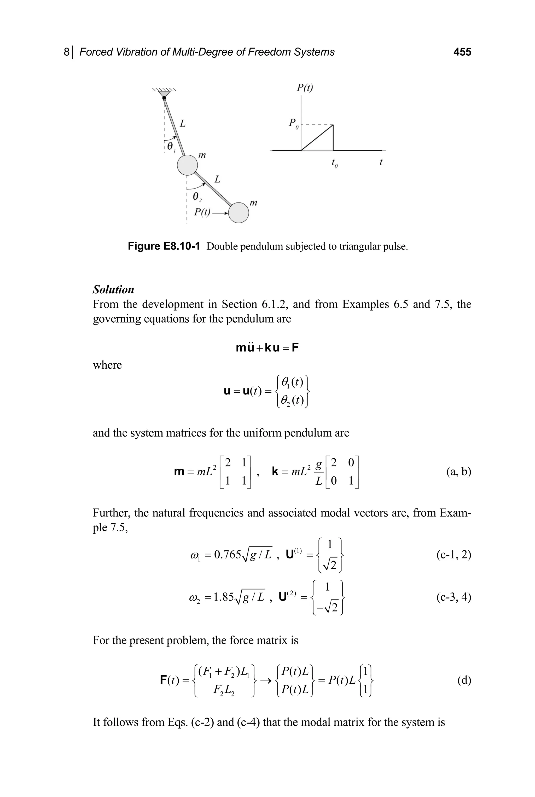
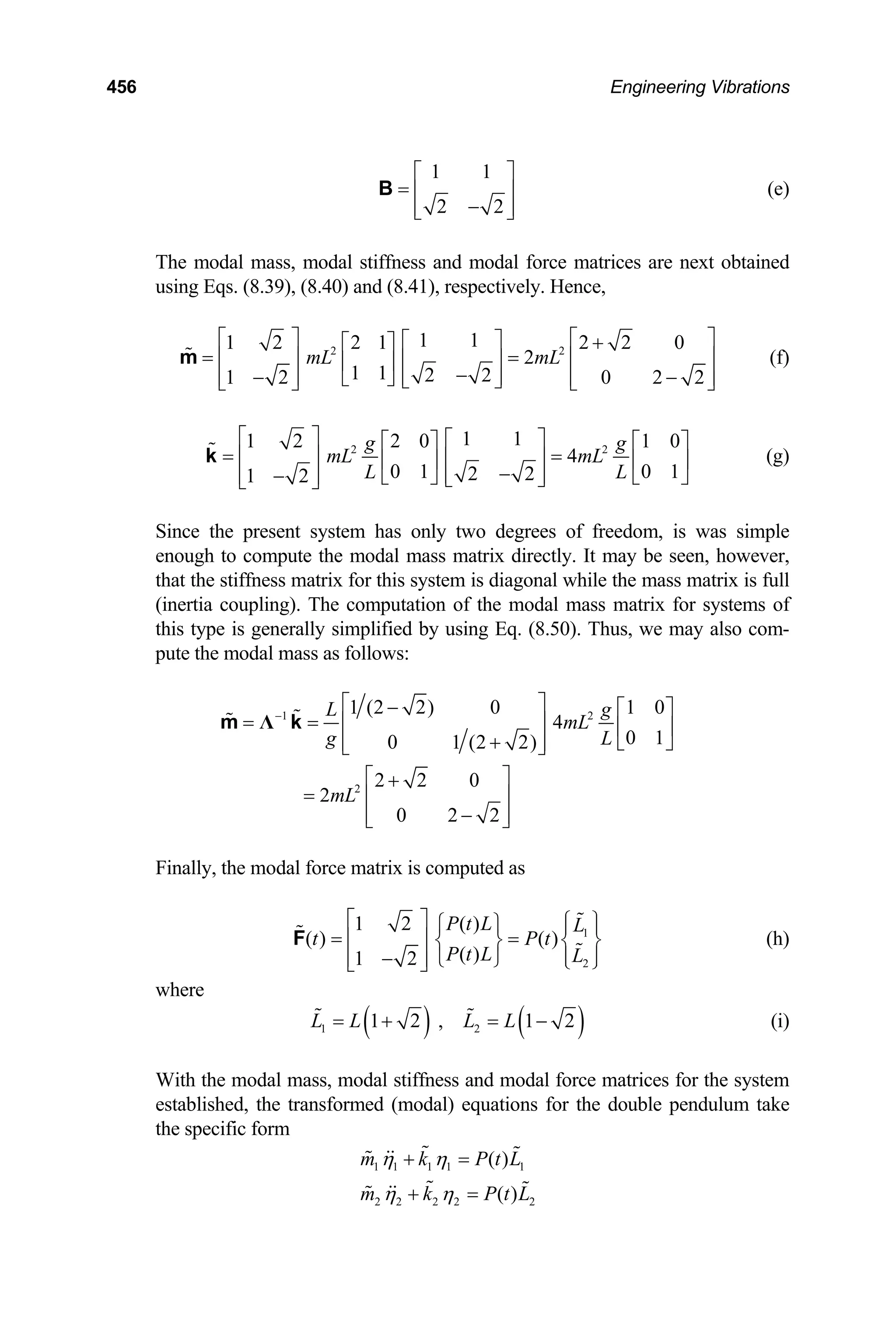
![8│ Forced Vibration of Multi-Degree of Freedom Systems 457
Figure E8.10-2 Decomposition of triangular pulse into the sum of three pulses.
or
2 2
1 1 1 1 1
2 2
2 2 2 2 2
( )
( )
f t
f t
η ω η ω
η ω η ω
+ =
+ =
(j)
where
2
1 1 1
2
2 2 2
( ) ( )
( ) ( )
1
2
f t P t L k
f t P t L
ω
ω
=
= k
(k)
Equations (j) may be solved for the modal displacements once we establish an
analytical form for the pulse P(t). Toward this end, the given triangular pulse
may be constructed as the sum of two ramp loads and a step load as shown in
Figure E8.10-2. Mathematically,
(l)
( ) ( ) ( )
( ) ( ) ( ) ( )
a b c
P t P t P t P t
= + +
where
( ) 0
0
( ) ( )
a P
P t t t
t
= H (m-1)
( )
( )
0 0
( ) 1 ( )
b
P t P t t t t
⎡ ⎤ 0
= −
⎣ ⎦ H −
0
(m-2)
( )
0
( ) ( )
c
P t P t t
= − −
H (m-3)
The response of each 1 d.o.f. system [the solutions to Eqs. (j)] is then the sum
of the responses to the individual pulses (m-1), (m-2) and (m-3). From the dis-
cussions of Sections 4.4, 4.5 and 4.6 we thus have that](https://image.slidesharecdn.com/engineeringvibrations-240713005818-b85f16c0/75/Engineering-Vibrations-Engineering-Vibrations-479-2048.jpg)
![458 Engineering Vibrations
[ ]
( ) ( ) ( )
1 1 1 1
0 1 1 0 1
1 1 0 1
0 1
( ) ( ) ( ) ( )
( ) ( ) ( )
a b c
t t t t
P L k P L
t t t t t
t k
η η η η
= + +
= − − −
R R S 0
−
(n-1)
and
[ ]
( ) ( ) ( )
2 2 2 2
0 2 2 0 2
2 2 0 2
0 2
( ) ( ) ( ) ( )
( ) ( ) ( )
a b c
t t t t
P L k P L
t t t t
t k
η η η η
= + +
= − − −
R R S 0
t
−
(n-2)
where, from Eqs. (4.32) and (4.39),
sin
( ) ( ) ( 1,2)
j
j
j
t
t t t j
ω
ω
⎡ ⎤
= − =
⎢ ⎥
⎢ ⎥
⎣ ⎦
R H (o)
(p)
0 0 0
( ) 1 cos ( ) ( ) ( 1,2
j j
t t t t t t j
ω
⎡ ⎤
− = − − − =
⎣ ⎦
S H )
The response of the double pendulum to the triangular pulse imparted on the
bottom mass is then found by substituting Eqs. (e) and (n) into Eq. (8.31). Do-
ing this, we find that
( )
( )
1 2
1 1
2 2 1 2
1 1
( ) ( )
( ) ( ) 2
2 2
t t
t t
η η
θ η
θ η η η
⎧ ⎫
+
⎡ ⎤
⎧ ⎫ ⎧ ⎫ ⎪ ⎪
= =
⎢ ⎥
⎨ ⎬ ⎨ ⎬ ⎨
−
−
⎢ ⎥
⎩ ⎭ ⎩ ⎭
⎬
⎪ ⎪
⎣ ⎦ ⎩ ⎭
(q)
and hence that
0 1 2 1 1 2 2
1
0 1 2
1 2 1 2
0 1 0 2
1 2 1 2
0 0
0 1 2
1 2 1 2
1 2
0
1 2
sin sin
( ) ( )
sin ( ) sin ( )
( ) ( )
P L L L t L t
t t t
t k k k k
P t t t
L L L L
t t t t
t k k k k
L L
P
k k
ω ω
θ
ω ω
ω ω
ω ω
⎡ ⎤
⎛ ⎞
= + − −
⎢ ⎥
⎜ ⎟
⎜ ⎟
⎢ ⎥
⎝ ⎠
⎣ ⎦
⎡ ⎤
⎛ ⎞ − −
− − + − − −
⎢ ⎥
⎜ ⎟
⎜ ⎟
⎢ ⎥
⎝ ⎠
⎣ ⎦
− + −
H
H
0
t
1 2
1 0 2 0 0
1 2
cos ( ) cos ( ) ( )
L L
t t t t t t
k k
ω ω
⎡ ⎤
− − − −
⎢ ⎥
⎢ ⎥
⎣ ⎦
H
(r-1)](https://image.slidesharecdn.com/engineeringvibrations-240713005818-b85f16c0/75/Engineering-Vibrations-Engineering-Vibrations-480-2048.jpg)
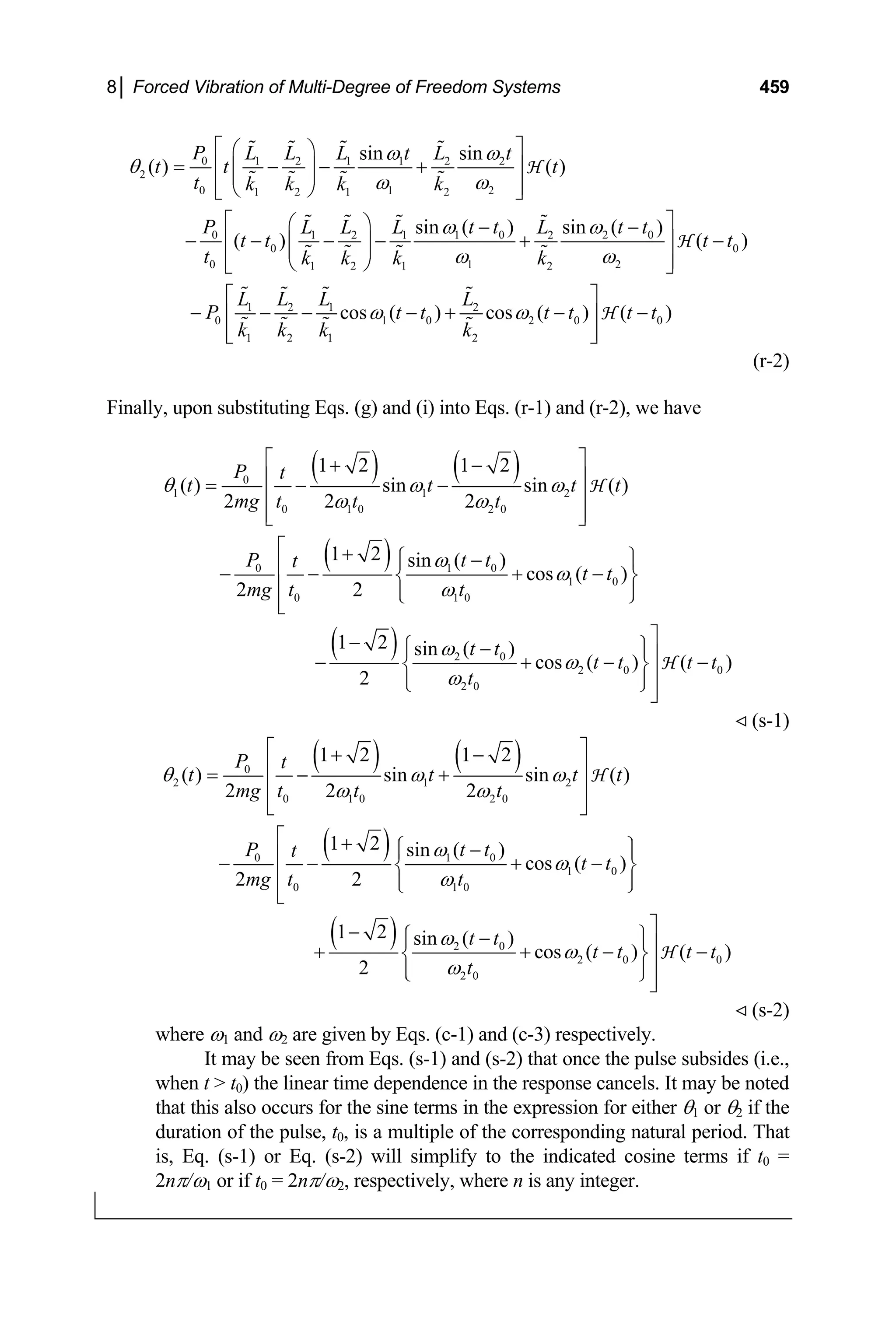
![460 Engineering Vibrations
Example 8.11
The tram of Examples 6.6 and 7.7 is shut down and at rest and, as a conse-
quence, the cable is slack and the controller is off when a wind gust strikes the
structure. Determine the motion of the tram if the effect of the wind gust may
be modeled as a rectangular pulse of magnitude F0 and duration τ.
Figure E8.11 Tram subjected to wind load.
Solution
For the specific system in question, the mass of the barrow is twice the mass of
the frame. That is, m2 = 2m1 = 2m. Further, for the present conditions, F1 = 0, M
= 0 and
[ ]
2 0
( ) ( ) ( )
F F t F t t τ
= = − −
H H (a)
The equation of motion of the system is then, from Example 6.6,
2
3 2 0 ( )
2 2 0 2 ( )
m mL u k u F t
mL mL mgL L F t
θ θ
⎡ ⎤ ⎧ ⎫ ⎡ ⎤ ⎧ ⎫ ⎧
+ =
⎫
⎨ ⎬ ⎨ ⎬ ⎨
⎢ ⎥ ⎢ ⎥
⎣ ⎦ ⎩ ⎭ ⎣ ⎦ ⎩ ⎭ ⎩
⎬
⎭
(b)
The natural frequencies and modes for this system were computed in Example
7.7 as
(1)
1 0 2
0
1
0.518 ,
0.366 g
ω ω
ω
⎧ ⎫
= = ⎨ ⎬
⎩ ⎭
U (c-1, 2)
(2)
2 0 2
0
1
1.93 ,
1.37 g
ω ω
ω
⎧ ⎫
= = ⎨ ⎬
−
⎩ ⎭
U (d-1, 2)
where the properties of the particular system under consideration are such that
2
0 k m g L
ω = = (e)](https://image.slidesharecdn.com/engineeringvibrations-240713005818-b85f16c0/75/Engineering-Vibrations-Engineering-Vibrations-482-2048.jpg)
![8│ Forced Vibration of Multi-Degree of Freedom Systems 461
The corresponding modal matrix is then
2
0 0
1 1
0.366 1.37 2
g g
ω ω
⎡ ⎤
= ⎢ ⎥
−
⎣ ⎦
B (f)
With the modal matrix established, we next compute the modal stiffness and
modal force matrices. Hence,
2
0
2
2
0 0
0
1 1
0
1 0.366
0.366 1.37
0 2
1 1.37
k
g
2
g g
mgL
g
ω
ω ω
ω
⎡ ⎤ ⎡ ⎤
⎡ ⎤
= ⎢ ⎥ ⎢ ⎥
⎢ ⎥ −
− ⎣ ⎦ ⎣ ⎦
⎣ ⎦
k
1.27 0
0 4.76
k
k
⎡ ⎤
⇒ = ⎢ ⎥
⎣ ⎦
k (g)
and
2
0
2
0
( ) 1.37 ( )
1 0.366
( ) 0.366 ( )
1 1.37
F t F t
g
L F t F t
g
ω
ω
⎡ ⎤ ⎧ ⎫ ⎧ ⎫
= =
⎨ ⎬ ⎨ ⎬
⎢ ⎥
−
− ⎩ ⎭ ⎩
⎣ ⎦
F
⎭
(h)
The modal equations are then
[ ]
[ ]
2 2 (1)
1 1 1 1 0
2 2 (2)
2 2 1 2 0
( ) ( ) ( ) ( )
( ) ( ) ( ) ( )
t t f t t
t t f t t
η ω η ω τ
η ω η ω τ
+ = − −
+ = − −
H H
H H
(i)
where
(1) (1)
0 0 1 0
(2) (2)
0 0 2 0
1.08
0.0769
f F k F k
f F k F k
= =
= = −
(j)
The solutions to equations (i) follow directly from Eq. (4.43). The modal dis-
placements are therefore
[ ] [ ]
{ }
[ ] [ ]
{ }
(1)
1 0 1 1 1 1
(2)
2 0 2 2 2 2
( ) 1 cos( ) ( ) 1 cos{ ( ) } ( )
( ) 1 cos( ) ( ) 1 cos{ ( ) } ( )
t f t t t t
t f t t t t
η ω φ ω τ φ τ
η ω φ ω τ φ τ
= − − − − − − −
= − − − − − − −
H H
H H
(k)
Transforming back to physical space gives the desired response. Hence,
1
2 2
0 0
1 2
2
1 2 0
1 1
( )
0.366 1.37 ( )
( )
( ) ( )
(0.366 1.37 )
t
u t
g g
t
t t
g
η
ω ω η
θ
η η
η η ω
⎡ ⎤
2
( )
t
⎧ ⎫
⎧ ⎫
=
⎨ ⎬ ⎨
⎢ ⎥
−
⎩ ⎭ ⎩
⎣
+
⎧ ⎫
= ⎨ ⎬
−
⎩ ⎭
⎬
⎭
⎦
(l)](https://image.slidesharecdn.com/engineeringvibrations-240713005818-b85f16c0/75/Engineering-Vibrations-Engineering-Vibrations-483-2048.jpg)
![462 Engineering Vibrations
Finally,
[ ]
[ ]
[ ]
0
0
0 1 0 1
0
0 1 0 1
( ) ( ) ( )
1.08cos(0.518 ) 0.0769cos(1.93 ) ( )
1.08cos{0.518 ( ) } 0.0769cos{1.93 ( ) } ( )
F
u t L t t
mg
F
t t t
mg
F
t t
mg
τ
ω φ ω φ
t
ω τ φ ω τ φ τ
= − −
− − − −
+ − − − − −
H H
H
H −
(m-1)
[ ]
[ ]
[ ]
0
0
0 1 0 1
0
0 1 0 1
( ) ( ) ( )
2
0.395cos(0.518 ) 0.105cos(1.93 ) ( )
0.395cos{0.518 ( ) } 0.105cos{1.93 ( ) } ( )
F
t t t
mg
F
t t t
mg
F
t t
mg
θ τ
ω φ ω φ
t
ω τ φ ω τ φ τ
= − −
− − + −
+ − − + − −
H H
H
H −
(m-2)
Example 8.12
The motorcycle of Examples 6.7 and 7.8 is traveling at constant speed v0 on a
horizontal road when it encounters a small depression in the road. If the depres-
sion is described by the function [ ]
0
( ) 1 cos(2 )
y h
ξ πξ λ
= − , determine the re-
sponse of the motorcycle that results from riding through the dip.
Figure E8.12-1 Motorcycle approaching depression in road.
Solution
The problem is similar to Example 4.7, but now for a three-degree of freedom
system with two wheels (Figure E8.12-2). The spatial equation that describes
the geometry of the depression is given as
[ ]
0
( ) 1 cos(2 )
y h
ξ πξ λ
= − (a)](https://image.slidesharecdn.com/engineeringvibrations-240713005818-b85f16c0/75/Engineering-Vibrations-Engineering-Vibrations-484-2048.jpg)
![8│ Forced Vibration of Multi-Degree of Freedom Systems 463
here h0 is the depth of the depression and λ is the corresponding length as
Figure E8.12-2 Equivalent system.
w
shown. Since the motorcycle moves at constant speed v0 the problem may be
viewed as if the vehicle is fixed and each base undergoes a prescribed vertical
motion, where the motion of the second base lags the first by the time incre-
ment
0
lag
t v L
= (b)
the first wheel encounters the depression at t 0 then, while passing through
(c)
ssing through the de
lag
ubstituting Eq. (c) into Eq. (a) gives the vertical motion of the front wheel as,
If =
the dip, the horizontal motion of the first wheel is
v t
ξ = 0
imilarly, while pa pression, the horizontal motion of the
S
second wheel is
( )
v t v t t
ξ ′
= = − (d)
0 0
S
[ ][ ]
01 0
( ) 1 cos ( ) ( )
y t h t t t t
= − Ω − −
H H (e)
λ
where
2 tλ
π
Ω = (f)
and
0
t v
λ λ
= (g)
the time it takes for the wheel to traverse th
) ( )
lag lag lag
t t t tλ
⎤
− − −
⎣ ⎦ ⎣ ⎦ (h)
is e depression. Likewise, the verti-
cal motion of the second wheel is given by
( ) 1 cos ( ) (
y t h t t t
⎡ ⎤ ⎡
= − Ω − −
H H
02 0](https://image.slidesharecdn.com/engineeringvibrations-240713005818-b85f16c0/75/Engineering-Vibrations-Engineering-Vibrations-485-2048.jpg)
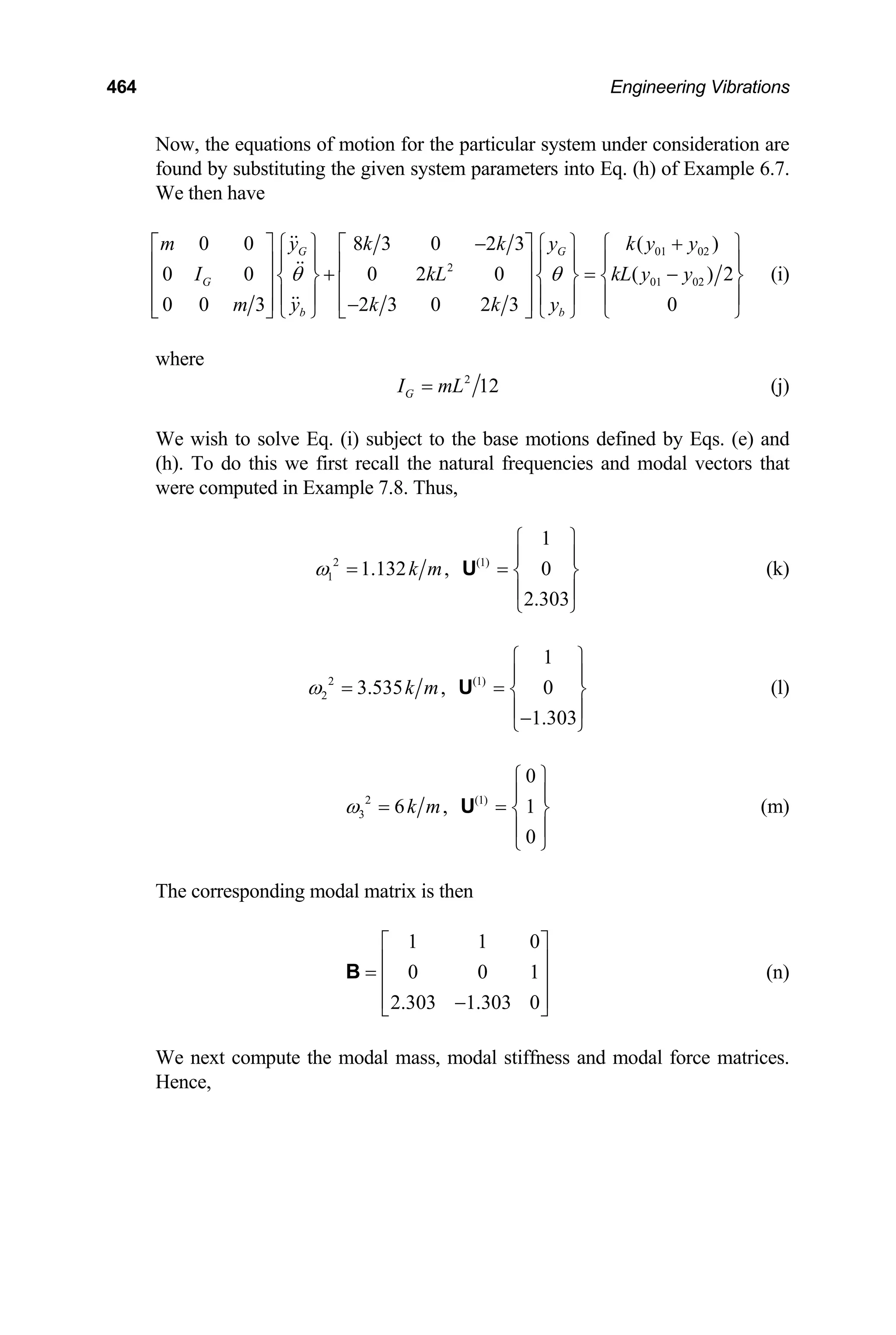
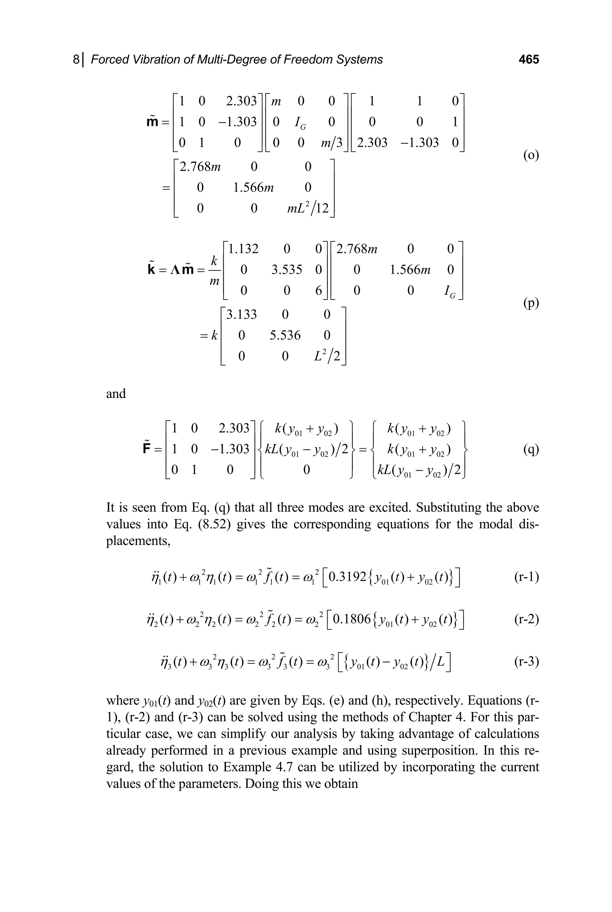
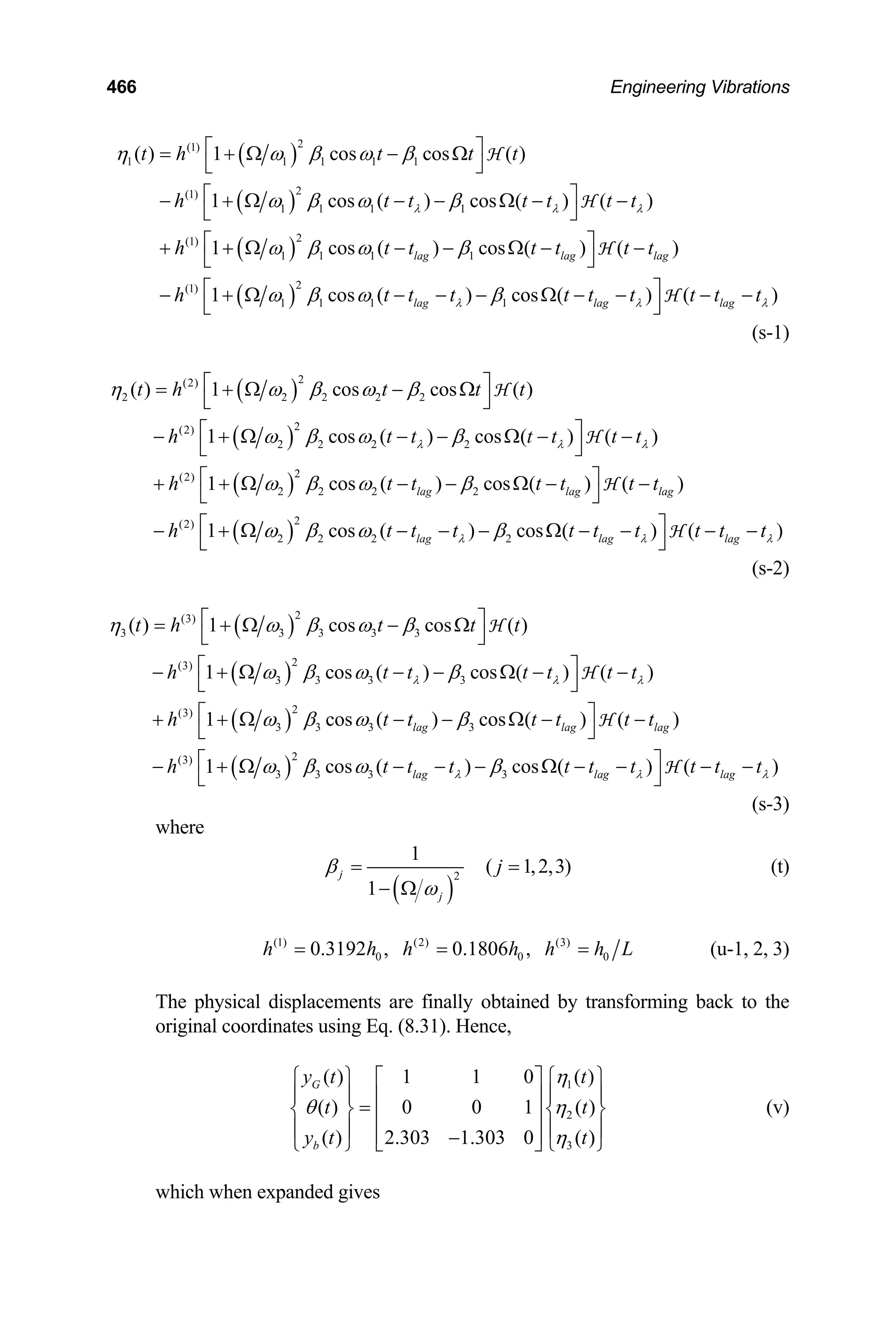
![8│ Forced Vibration of Multi-Degree of Freedom Systems 467
1 2
( ) ( ) ( )
G
y t t t
η η
= + (w-1)
3
( ) ( )
t t
θ η
= (w-2)
1 2
( ) 2.303 ( ) 1.303 ( )
b
y t t t
η η
= − (w-3)
where η1(t), η2(t) and η3(t) are given by Eqs. (s-1), (s-2) and (s-3), respectively.
It is seen that the rotational coordinate is a modal coordinate. Let’s examine the
motion of the rider in detail.
The detailed response of the rider is found by substituting Eqs. (s-1) and
(s-2) into Eq. (w-3) and evaluating the resulting expression when the front
wheel is rolling through the depression (0 t tλ), after it passes the dip but be-
fore the second wheel encounters the depression (tλ t tlag), when the second
wheel rolls through the depression (tlag t tlag + tλ) and after the second wheel
passes the dip (t tlag). The explicit forms are detailed below.
0 t tλ :
During the interval when the first wheel is going through the depression, the
motion of the rider is
( ) ( )
( )
( ) ( )
0 0
2 2
0 0 0
2 2
0 0
0 0
2 2
0 0
( ) 1 0.7351 0.2353
cos 2
2 1 34.87 1 11.17
25.63 2.628
cos(1.064 ) cos(1.880 )
1 34.87 1 11.17
b
y t
v t
h v v
v v
t t
v v
π ω
ω ω
⎡ ⎤
⎢ ⎥
= + −
⎢ ⎥
− −
⎣ ⎦
+ −
− −
(x-1)
where
0
0
0
v
v
ω λ
= (y)
and
0 k m
ω = (z)
tλ t tlag :
After the first wheel has gone through the depression, but before the second
wheel begins its transversal, the motion of the rider is
( )
[ ]
( )
[ ]
2
0
0 0
2
0 0
2
0
0 0
2
0
( ) 25.63
cos(1.064 ) cos{1.064 ( )}
1 34.87
2.628
cos(1.880 ) cos{1.880 ( )}
1 11.17
b
y t v
t t
h v
v
t t
t
v
λ
λ
ω ω
ω ω
= − −
−
− − −
−
t
(x-2)](https://image.slidesharecdn.com/engineeringvibrations-240713005818-b85f16c0/75/Engineering-Vibrations-Engineering-Vibrations-489-2048.jpg)
![468 Engineering Vibrations
tlag t tlag + tλ :
As the second wheel rolls through the depression the motion of the rider is
given by
( ) ( )
( )
( )
0 0
2 2
0 0 0
2
0
0 0 0
2
0
2
0
0 0
2
0
( ) 1 0.7351 0.2353
cos{2 ( )}
2 1 34.87 1 11.17
25.63
cos(1.064 ) cos{1.064 ( )} cos{1.064 ( )}
1 34.87
2.628
cos(1.880 ) cos{1.880 ( )} c
1 11.17
b
lag
lag
y t
v t t
h v v
v
t t t t
v
v
t t t
v
λ
λ
π ω
ω ω ω
ω ω
⎡ ⎤
⎢ ⎥
= + − −
⎢ ⎥
− −
⎣ ⎦
⎡ ⎤
+ − − +
⎣ ⎦
−
− − − +
−
0
os{1.880 ( )}
lag
t t
ω
⎡ ⎤
−
⎣ ⎦
t
−
(x-3)
t tlag :
After the second wheel has passed the depression the motion of the rider is
( )
[ ]
{
}
( )
[ ]
{
2
0
0 0
2
0 0
0 0
2
0
0 0
2
0
0 0
( ) 25.63
cos(1.064 ) cos{1.064 ( )}
1 34.87
cos{1.064 ( )} cos{1.064 ( )}
2.628
cos(1.880 ) cos{1.880 ( )}
1 11.17
cos{1.880 ( )} cos{1.880 (
b
lag lag
lag lag
y t v
t t t
h v
t t t t t
v
t t t
v
t t t t t
λ
λ
λ
ω ω
ω ω
ω ω
ω ω
= − −
−
⎡ ⎤
+ − − − −
⎣ ⎦
− − −
−
+ − − − − }
)}
λ
⎡ ⎤
⎣ ⎦
(x-4)
8.6 MODE ISOLATION
In certain situations it may be desirable to excite one particular mode of a system, but
none of the other modes. In the present section we examine how this may be accom-
plished.
Recall from Section 8.2.2 that when a vector v is operated on by a linear trans-
formation R, it results in a vector such that
,
v
=
v R v](https://image.slidesharecdn.com/engineeringvibrations-240713005818-b85f16c0/75/Engineering-Vibrations-Engineering-Vibrations-490-2048.jpg)
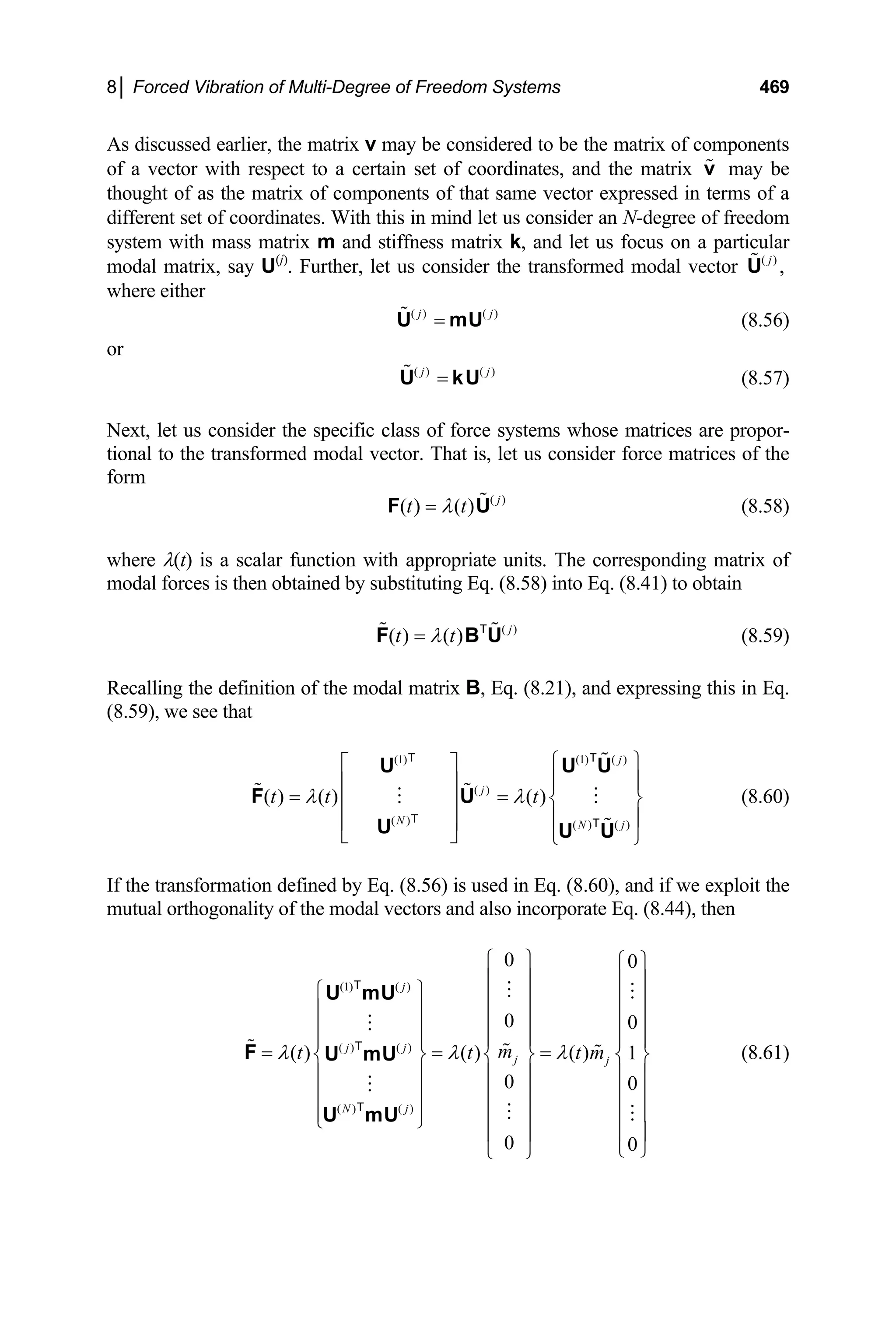
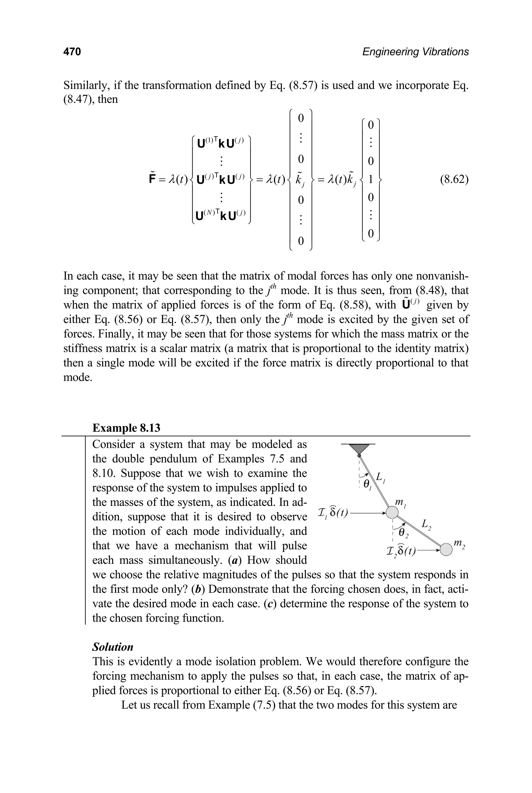
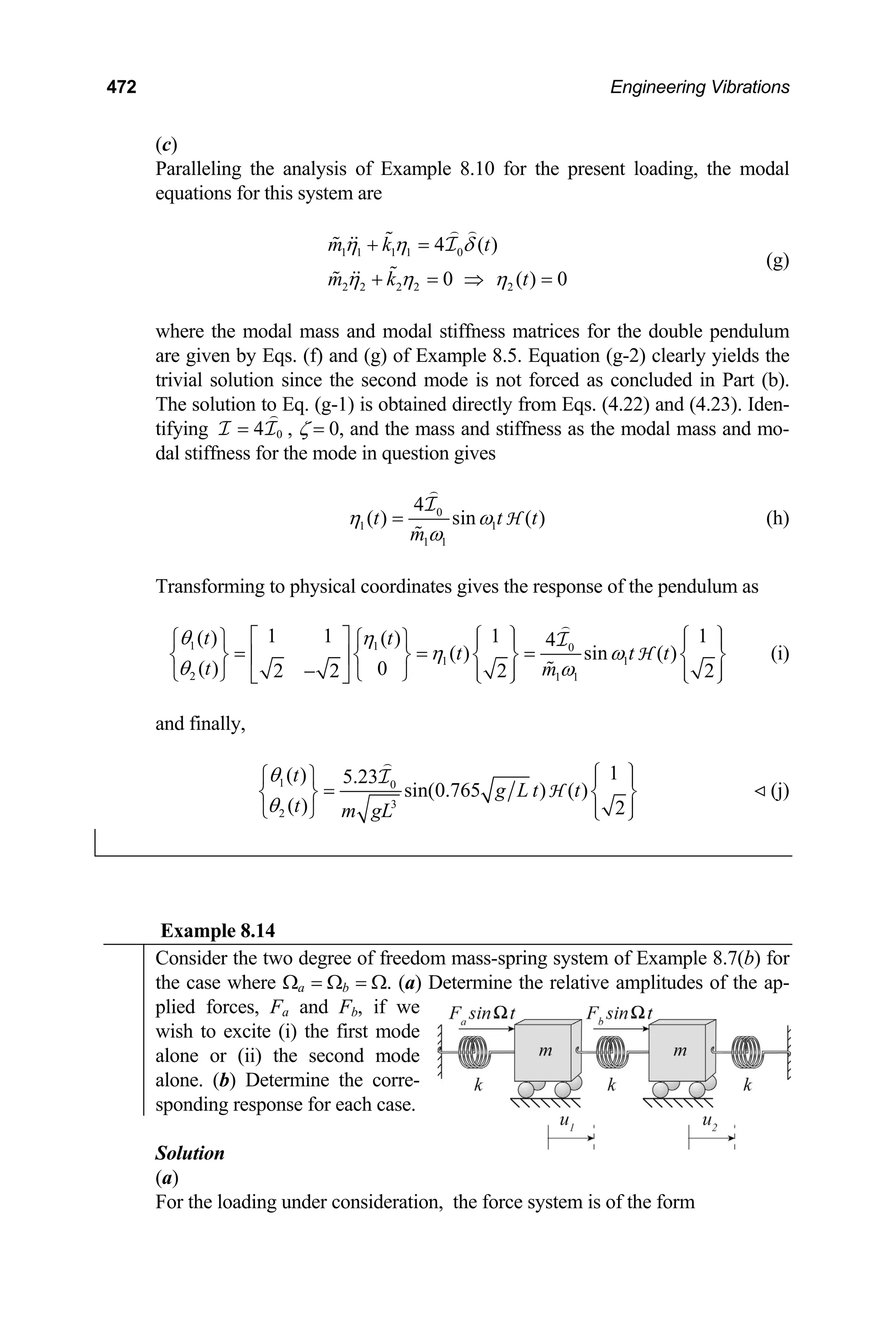
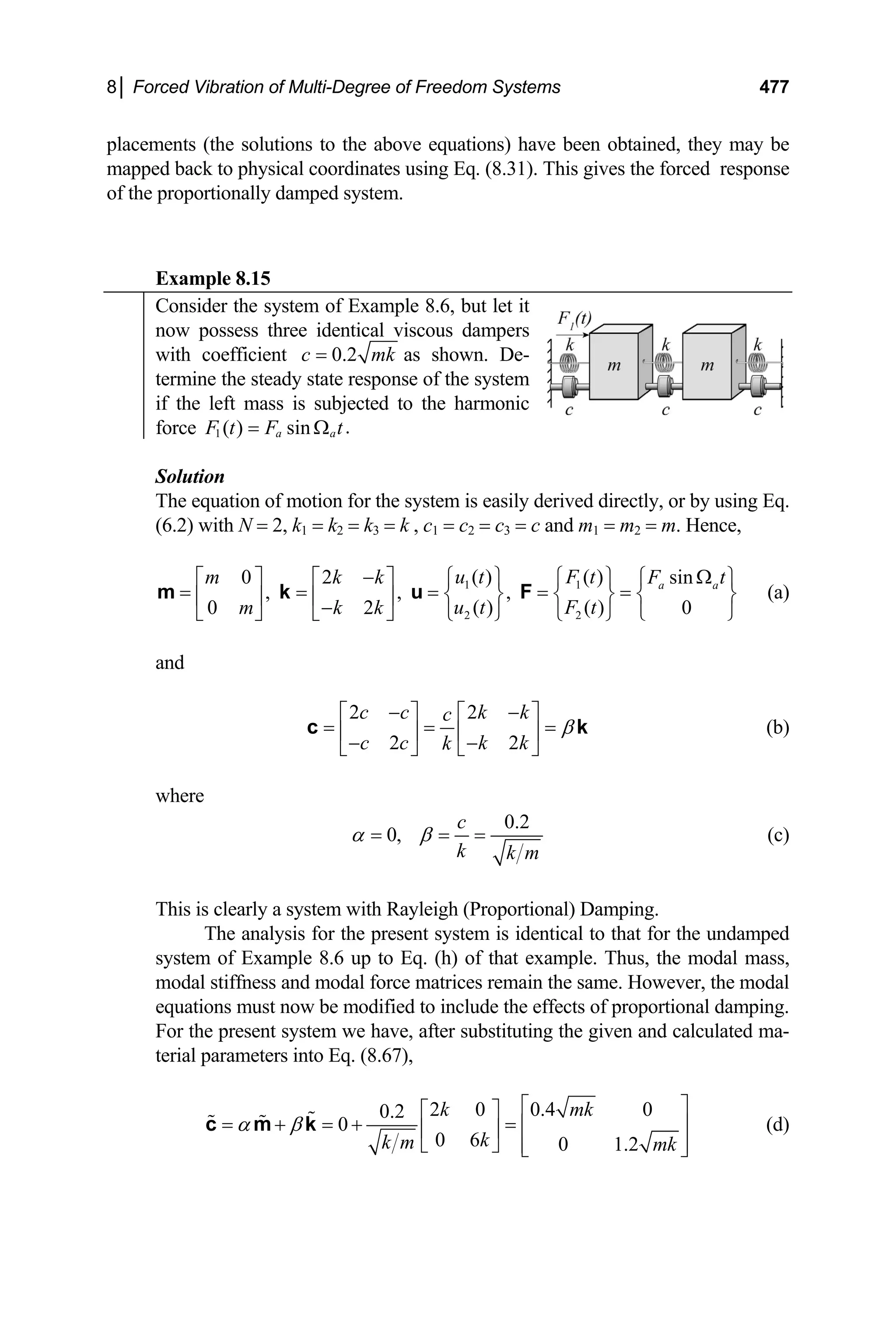
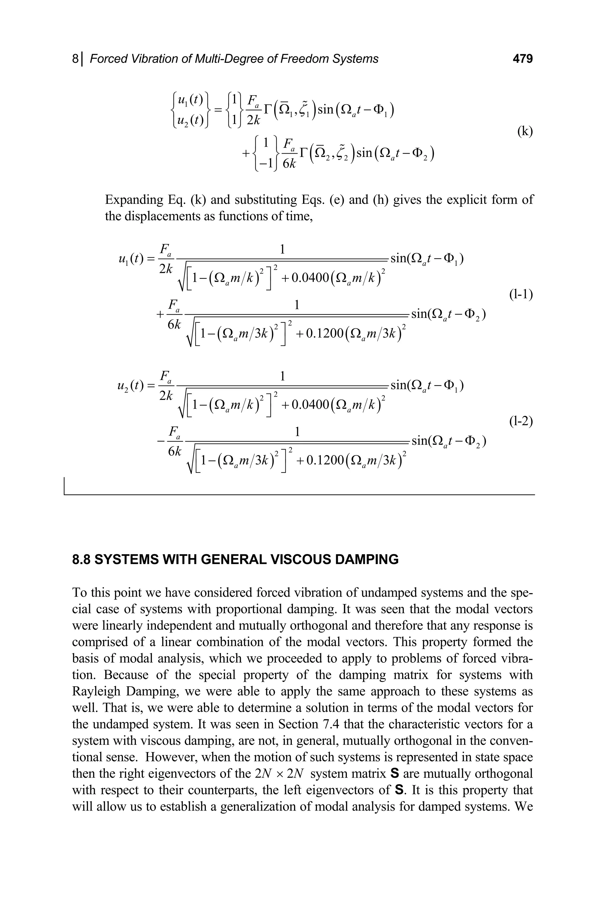
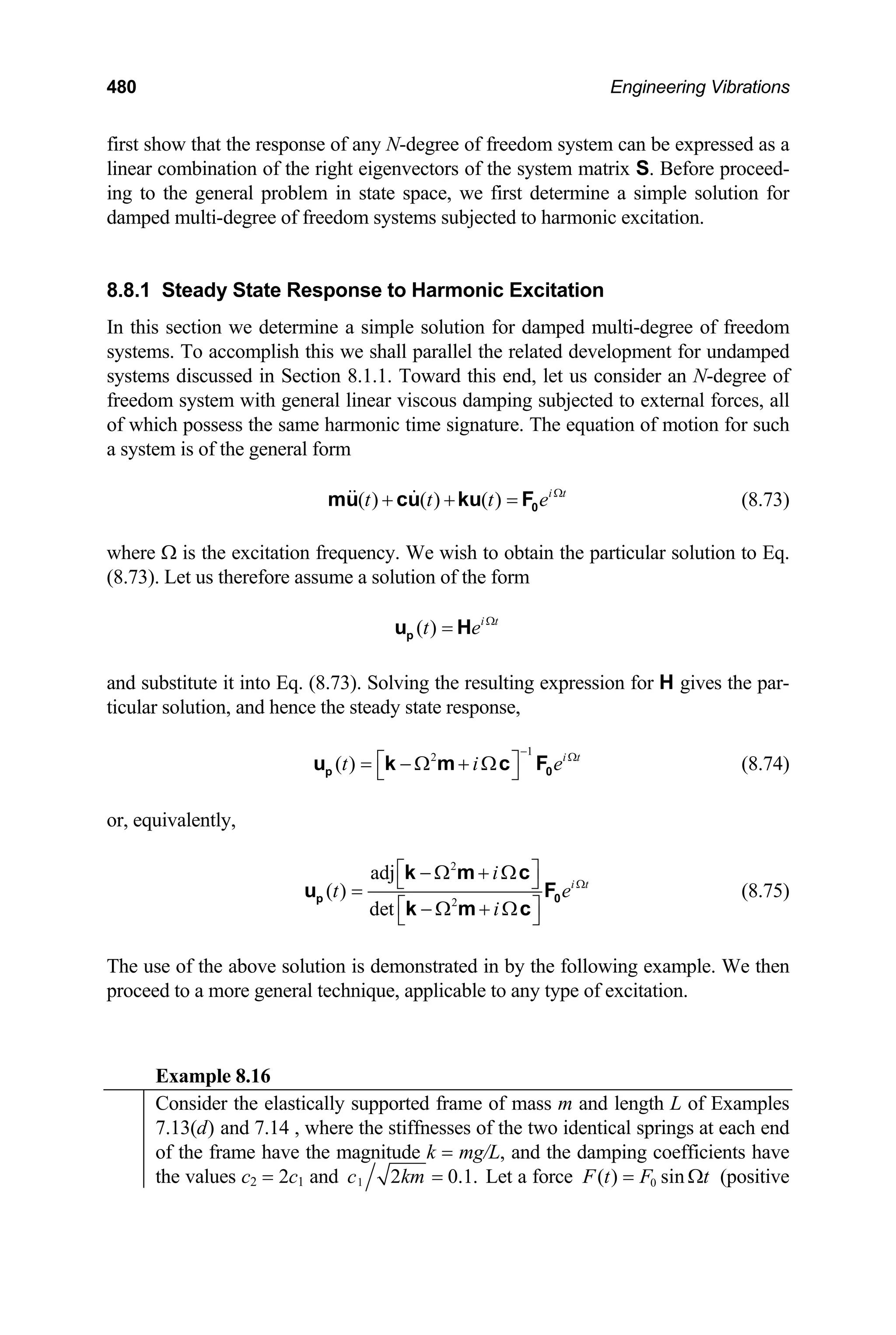
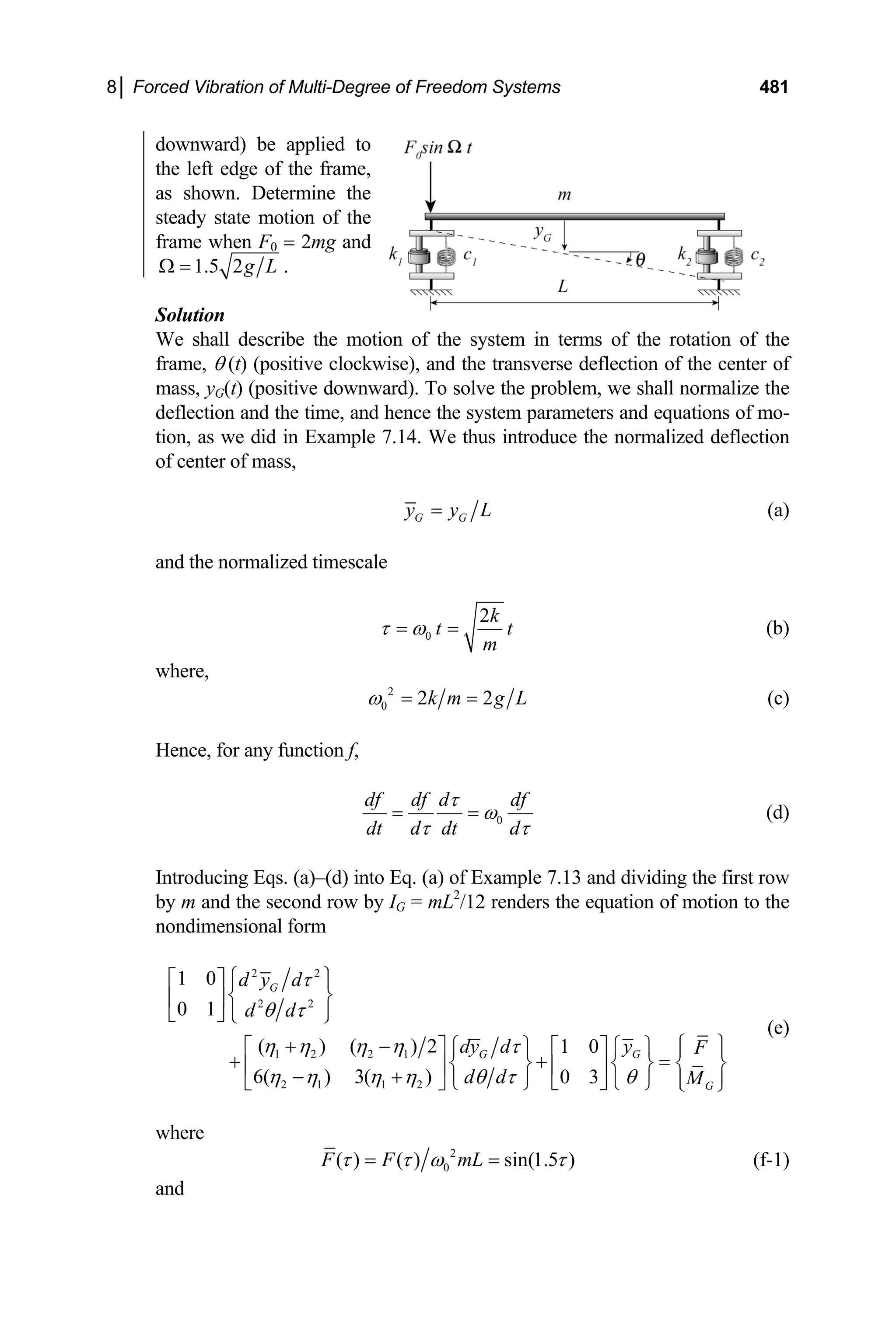
![482 Engineering Vibrations
2 2 2
0 0
( ) ( ) 12 ( ) 6sin(1.5 )
G G G G
M M I M mL
τ τ ω τ ω τ
= = = (f-2)
are the normalized resultant applied force and moment about an axis through G.
For the particular system in question, η1 = 0.5 and η2 = 1.0. It then follows that,
for the system in question, the complex form of the normalized force vector is
1.5
1
( )
6
i
t e τ
⎧ ⎫
= ⎨ ⎬
⎩ ⎭
F (g)
Further, for the given parameters,
2 ( 1.25 2.25 ) 0.375
4.5 (0.75 6.75 )
i i
i
i i
− +
⎡ ⎤
⎡ ⎤
− Ω + Ω = ⎢ ⎥
⎣ ⎦ +
⎣ ⎦
k m c (h)
We next compute the inverse of the above matrix using the MATLAB “inv” fa-
cility. Hence,
1
2 (0.2220 0.3637 ) (0.0100 0.0213 )
(0.1196 0.2558 ) (0.0113 0.1611 )
i i
i
i i
− − + +
⎡ ⎤
⎡ ⎤
− Ω + Ω = ⎢ ⎥
⎣ ⎦ + −
⎣ ⎦
k m c (i)
The complex form of the response is then found by substituting Eqs. (g) and (i)
into Eq. (8.74). Doing this we obtain
1.5
1.5
( ) (0.2220 0.3637 ) (0.0100 0.0213 ) 1
( ) (0.1196 0.2558 ) (0.0113 0.1611 ) 6
(0.1622 0.2358 )
(0.1871 0.7109 )
G i
i
y t i i
e
t i i
i
e
i
τ
τ
θ
− + +
⎧ ⎫ ⎡ ⎤ ⎧ ⎫
=
⎨ ⎬ ⎨ ⎬
⎢ ⎥
+ −
⎩ ⎭ ⎣ ⎦ ⎩ ⎭
− +
⎧ ⎫
= ⎨ ⎬
−
⎩ ⎭
(j)
Restating the exponential using Euler’s Formula and carrying through the indi-
cated multiplications gives
( ) [ 0.1622cos(1.5 ) 0.2358sin(1.5 )]
[0.2358cos(1.5 ) 0.1622sin(1.5 )]
G
y t
i
τ τ
τ τ
= − +
− +
(k-1)
( ) [0.1871cos(1.5 ) 0.7109sin(1.5 )]
[ 0.7109cos(1.5 ) 0.1871sin(1.5 )]
t
i
θ τ τ
τ τ
= +
+ − +
(k-2)
Since the excitation is a sine function, the imaginary part of the above solution
corresponds to the response of the system. The steady state response of the sys-
tem is then](https://image.slidesharecdn.com/engineeringvibrations-240713005818-b85f16c0/75/Engineering-Vibrations-Engineering-Vibrations-504-2048.jpg)
![8│ Forced Vibration of Multi-Degree of Freedom Systems 483
0
( ) / [0.2358cos(1.5 ) 0.1622sin(1.5 )]
G
y t L t t
0
ω ω
= − + (l-1)
0
( ) 0.7109cos(1.5 ) 0.1871sin(1.5 )
t t 0t
θ ω
=− + ω (l-2)
8.8.2 Eigenvector Expansion
The solution presented in Section 8.8.1 is restricted to harmonic excitation. In this
section we develop a procedure for damped systems that is a generalization of modal
analysis, and is applicable to any type of loading. To accomplish this we must repre-
sent the forced vibration problem in its corresponding state space, as we did for free
vibrations of damped systems in Section 7.4.2. We then seek to express the response
of the forced system in terms of the (right) eigenvectors of the state space system
matrix computed for the associated free vibration problem.
In order to express the state vector in terms of the right eigenvectors of the sys-
tem matrix S defined by Eq. (7.61) we must first show that the vectors are linearly
independent. This is done by generalizing the development of Section 8.3.1 in the
context of the state space representation. Toward this end, let us consider the sets of
2N 1 (complex) right and left eigenvectors of the (nonsymmetric) system matrix S,
×
{ } { }
( ) ( )
ˆ ˆ
1,2,...,2 and 1,2,...,2
j j
j N j
= =
U W N
respectively, where S is defined by Eq. (7.61) and and are defined by Eqs.
(7.63), (7.64) and (7.69). If the right eigenvectors are linearly independent then the
equation
Û Ŵ
2
( )
1
ˆ 0
N
j
j
j
a
=
=
∑ U (8.76)
is satisfied only if all aj = 0 (j = 1, 2, …, N) . We proceed to show that this is the case.
Let us next multiply Eq. (8.76) by This gives
( )
ˆ .
l
W
T
2
( ) ( )
1
ˆ ˆ 0
N
l j
j
j
a
=
=
∑ W U
T
(8.77)
We next incorporate the orthogonality relation stated by Eq. (7.75) into Eq. (8.77).
This results in the statement
( ) ( )
ˆ ˆ 0
l l
l
a =
W U
T
(8.78)](https://image.slidesharecdn.com/engineeringvibrations-240713005818-b85f16c0/75/Engineering-Vibrations-Engineering-Vibrations-505-2048.jpg)
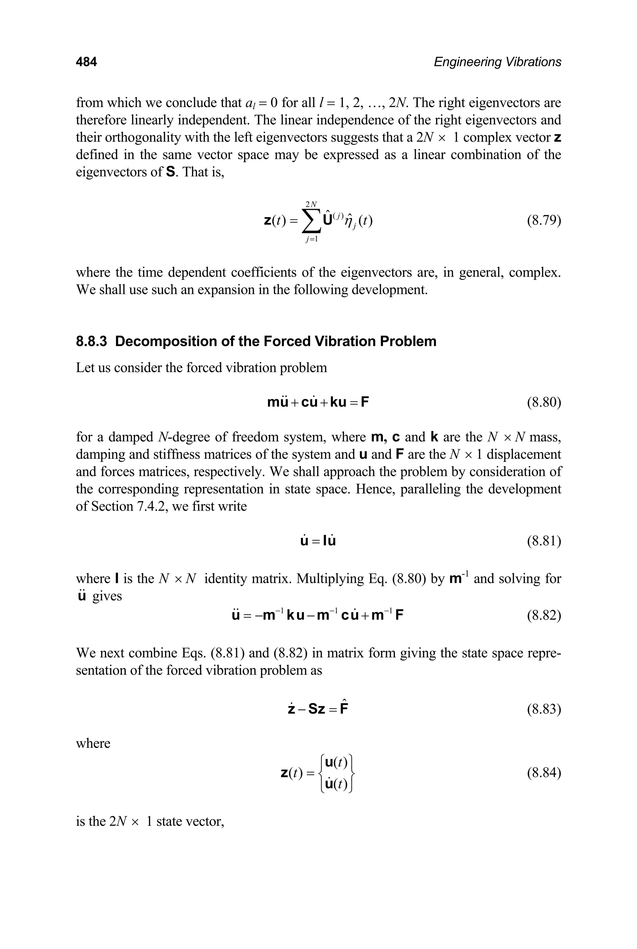
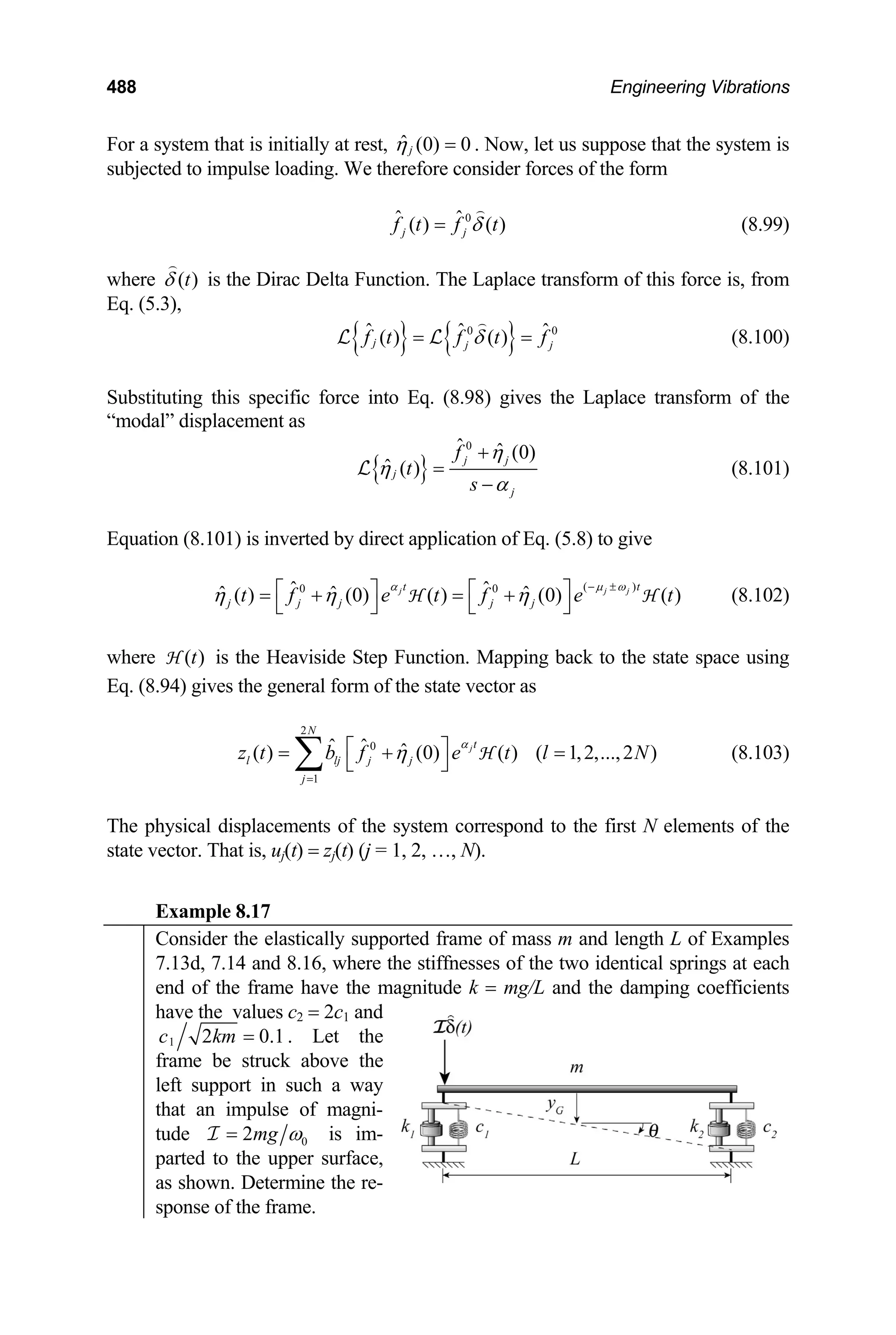
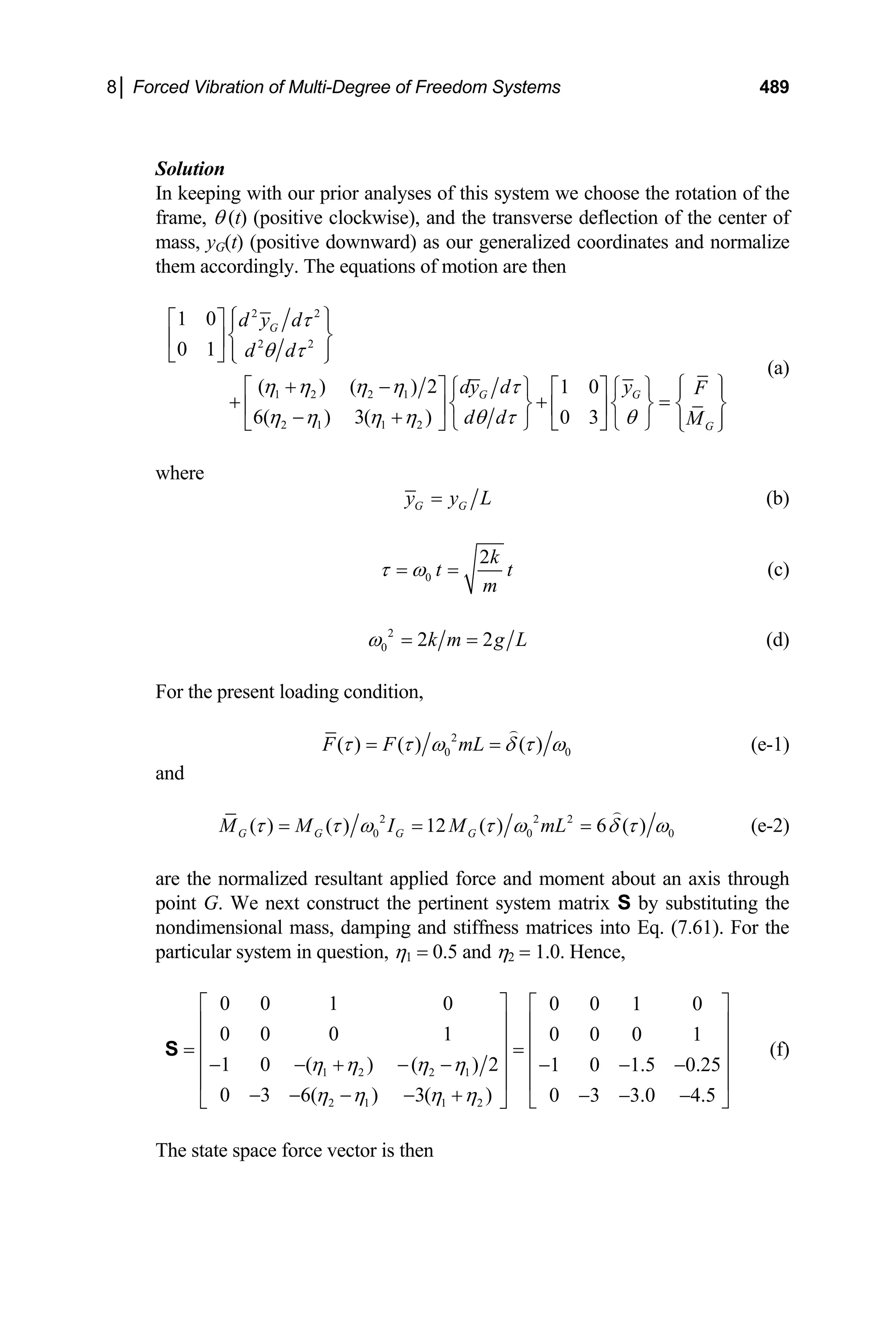
![490 Engineering Vibrations
0
0
0 0 0
0
0 0 0
( ) ( )
ˆ( )
( )
1 0 1
( )
( )
0 1 6
G
G
F
F
M
M
τ δ τ
τ
τ ω
τ
τ
⎧ ⎫
⎡ ⎤ ⎧ ⎫
⎪ ⎪
⎢ ⎥ ⎪ ⎪
⎧ ⎫
⎪ ⎪ ⎪ ⎪ ⎪ ⎪
⎢ ⎥
= = =
⎨ ⎬ ⎨ ⎬ ⎨ ⎬
⎢ ⎥ ⎪ ⎪
⎩ ⎭ ⎪ ⎪ ⎪ ⎪
⎢ ⎥ ⎪ ⎪ ⎪ ⎪
⎣ ⎦ ⎩ ⎭
⎩ ⎭
F (g)
With the problem formulated, we next proceed to calculate the response. Using
the MATLAB “eig” routine to solve the eigenvalue problem gives the eigenval-
ues of S,
ˆ 4.035, (0.6810 0.8673 ), (0.6810 0.8673 ), 0.6129
i i
α = − − − − + − (h)
and the corresponding matrix of (right) eigenvectors
(i)
0.0216 (0.4001 0.1545 ) (0.4001 0.1545 ) 0.2714
0.2401 (0.3193 0.4066 ) (0.3193 0.4066 ) 0.8082
ˆ
0.0871 (0.4065 0.2418 ) (0.4065 0.2418 ) 0.1664
0.9666 0.5701 0.5701 0.4954
i i
i i
i i
+ −
⎡ ⎤
⎢ ⎥
− + − −
⎢ ⎥
=
⎢ ⎥
− − − − + −
⎢ ⎥
− −
⎣ ⎦
B
[Note that MATLAB normalizes the eigenvectors in the conventional sense, as
per Eq. (7.39).] We next compute the inverse of the “modal matrix” using the
MATLAB “inv” routine. Hence,
1
0.3068 0.8508 1.235 1.142
(0.3644 1.052 ) ( 0.2564 0.2162 ) (0.6640 1.032 ) (0.0043 0.1232 )
(0.3644 1.052 ) (0.2564 0.2162 ) ( 0.6640 1.032 ) (0.0043 0.1232 )
1.437 1.070 0.8809 0.2186
ˆ
i i i
i i i i
−
− − − −
− − + − + +
+ − + − + −
=
⎡ ⎤
⎢ ⎥
⎢ ⎥
⎢ ⎥
⎢ ⎥
⎣ ⎦
B
i
(j)
With the above established, we now compute the “modal” forces, using Eq.
(8.96). Hence,
0.3068 0.8508 1.235 1.142
(0.3644 1.052 ) ( 0.2564 0.2162 ) (0.6640 1.032 ) (0.0043 0.1232 )
(0.3644 1.052 ) (0.2564 0.2162 ) ( 0.6640 1.032 ) (0.0043 0.1232 )
1.437 1.070 0.8809 0.2186
ˆ( )
0
0
1
6
i i i i
i i i i
t
− − − −
− − + − + +
+ − + − + −
=
⎧
⎡ ⎤
⎢ ⎥
⎢ ⎥ ⎨
⎢ ⎥
⎢ ⎥
⎣ ⎦
f
0
( )
δ τ
ω
⎫
⎪ ⎪
⎪ ⎪
⎬
⎪ ⎪
⎪ ⎪
⎩ ⎭
which, after carrying through the indicated multiplications gives](https://image.slidesharecdn.com/engineeringvibrations-240713005818-b85f16c0/75/Engineering-Vibrations-Engineering-Vibrations-512-2048.jpg)
![8│ Forced Vibration of Multi-Degree of Freedom Systems 491
0
8.0839
0.6381 0.2929 ( )
ˆ( )
0.6381 0.2929
2.1925
i
t
i
δ τ
ω
−
⎧ ⎫
⎪ ⎪
− −
⎪
= ⎨
− +
⎪ ⎪
⎪ ⎪
⎩ ⎭
⎪
⎬
f (k)
The “modal” displacements are next found by substituting Eq. (k) into Eq.
(8.102). Hence,
4.035
0 1
(0.6381 0.2929 )
0 2
(0.6381 0.2929 )
0 3
0.6129
0 4
ˆ ( ) 8.084 ( )
ˆ ( ) (0.6381 0.2929 ) ( )
ˆ ( ) (0.6381 0.2929 ) ( )
ˆ ( ) 2.193 ( )
i
i
e
i e
i e
e
τ
τ
τ
τ
ω η τ τ
ω η τ τ
ω η τ τ
ω η τ τ
−
− +
− −
−
= −
= − +
= − −
=
H
H
H
H
(l)
To obtain the physical displacements, we map back to the state space as fol-
lows:
4
0 0 1
1
4.035
(0.6381 0.2929 )
(0.6381 0.2929 )
0.6129
ˆ ˆ
( ) ( )
0.02160( 8.084) ( )
(0.4001 0.1545 )(0.6381 0.2929 ) ( )
(0.4001 0.1545 )(0.6381 0.2929 ) ( )
0.2714(2.193) ( )
G j j
j
i
i
y b
e
i i e
i i e
e
τ
τ
τ
τ
ω τ ω η τ
τ
τ
τ
τ
=
−
− +
− −
−
=
= −
− + +
+ − −
+
∑ H
H
H
H
H
4
0 0 2
1
4.035
(0.6381 0.2929 )
(0.6381 0.2929 )
0.6129
ˆ ˆ
( ) ( ) ( )
0.2401( 8.084) ( )
(0.3193 0.4066 )( 0.6381 0.2929 ) ( )
(0.3193 0.4066 )( 0.6381 0.2929 ) ( )
0.8082(2.193) ( )
j j
j
i
i
b
e
i i e
i i e
e
τ
τ
τ
τ
ω θ τ ω η τ τ
τ
τ
τ
τ
=
−
− +
− −
−
=
= −
− + − −
− − − +
+
∑ H
H
H
H
H
Carrying through the indicated multiplication gives the response of the frame as
[ ]
0 0
0
4.035 0.6129
0
0.6810
0 0
( ) 0.1746 ( ) 0.5952 ( )
0.4200cos(0.8673 ) 0.4316sin(0.8673 ) ( )
t t
G
t
y t L e t e t
e t
ω ω
ω
ω
ω ω
− −
−
= − +
− −
H H
H
t t
(m-1)](https://image.slidesharecdn.com/engineeringvibrations-240713005818-b85f16c0/75/Engineering-Vibrations-Engineering-Vibrations-513-2048.jpg)
![492 Engineering Vibrations
(m-2)
[ ]
0 0
0
4.035 0.6129
0
0.6810
0 0
( ) 1.941 ( ) 1.772 ( )
0.1612cos(0.8673 ) 0.7060sin(0.8673 ) ( )
t t
t
t e t e t
e t
ω ω
ω
ω θ
ω ω
− −
−
= − +
+ −
H H
H
t t
Arbitrary Loading
The response of a system to arbitrary loading is found by paralleling the arguments of
Section 4.3 and incorporating the impulse response defined above to obtain the corre-
sponding “modal displacements.” Doing this we find that, for a system initially at
rest,
(8.104)
( )
0
ˆ
ˆ ( ) ( ) ( )
j
t
t
j j
t f e d
α τ
η τ τ
−
=
∫ H t
The above expression may be evaluated for any given ˆ ( ).
j
f τ Once the “modal dis-
placements” are determined for a given set of forces, they may be mapped back to the
state space using Eq. (8.94) to obtain the state vector z(t). The physical displacements
of the system then correspond to the first N elements of this vector. Equation (8.94) is
evaluated for step loading and ramp loading below.
Step Loading
Consider forces of the form
(8.105)
0
ˆ ˆ
( ) ( )
j j
f t f t
= H
where (complex) constant. Substituting the above step load function into
Eq. (8.104) and evaluating the resulting integral gives the corresponding dis-
placements
0
ˆ
j
f =
0
ˆ
ˆ ( ) 1 ( )
jt
j
j
j
f
t e
α
η
α
⎡ ⎤
= −
⎣ ⎦
H t (8.106)
Ramp Loading
Consider forces of the form
(8.107)
0
ˆ ˆ
( ) ( )
j j
f t f t t
= H
where (complex) constant. Substituting the above ramp load function into
Eq. (8.104) and evaluating the resulting integral gives the corresponding dis-
placements
0
ˆ
j
f =](https://image.slidesharecdn.com/engineeringvibrations-240713005818-b85f16c0/75/Engineering-Vibrations-Engineering-Vibrations-514-2048.jpg)
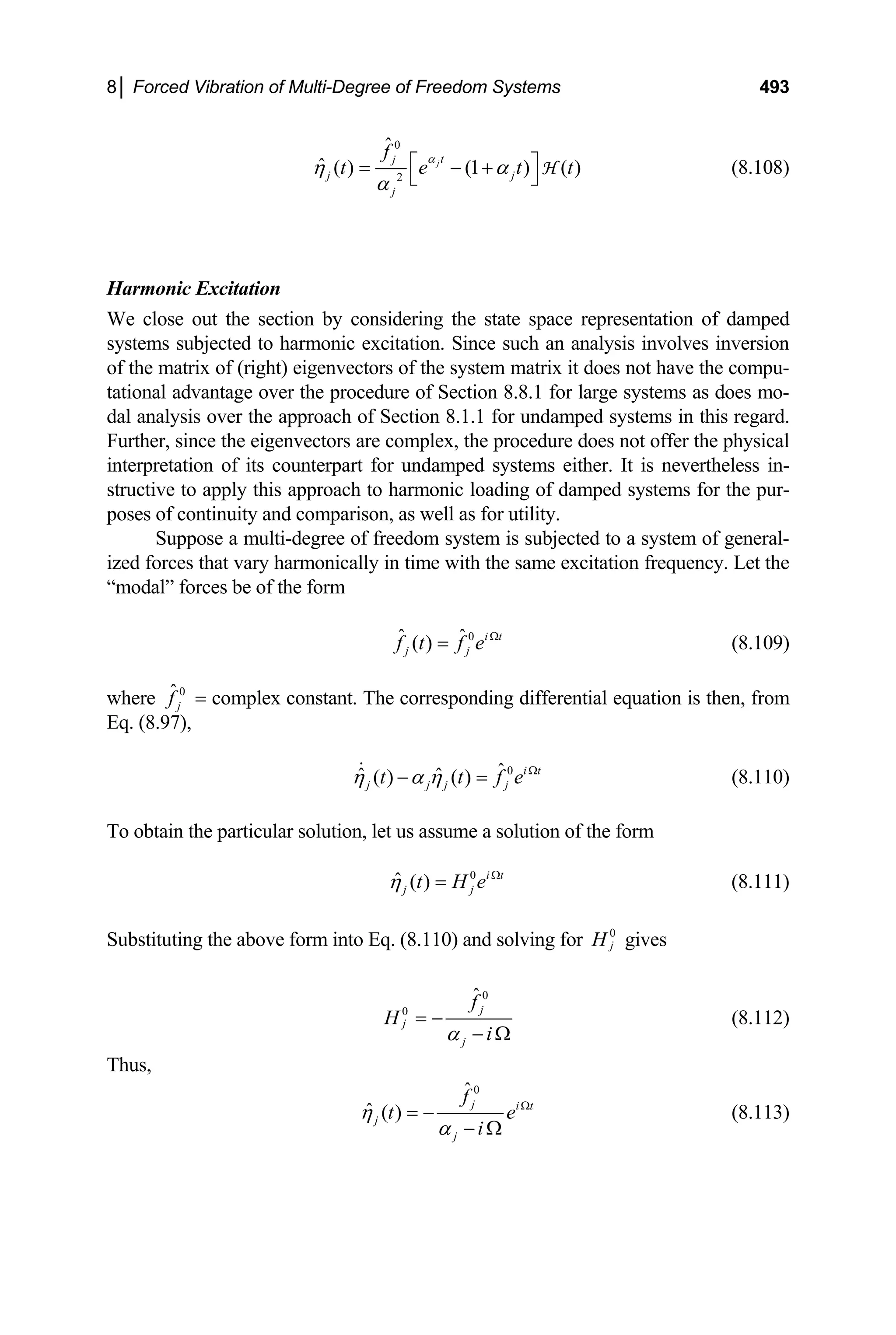
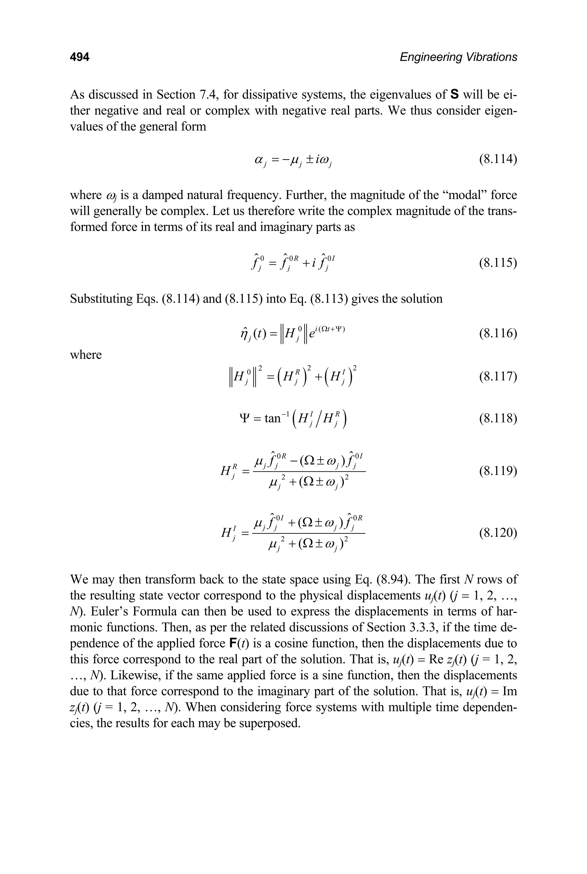
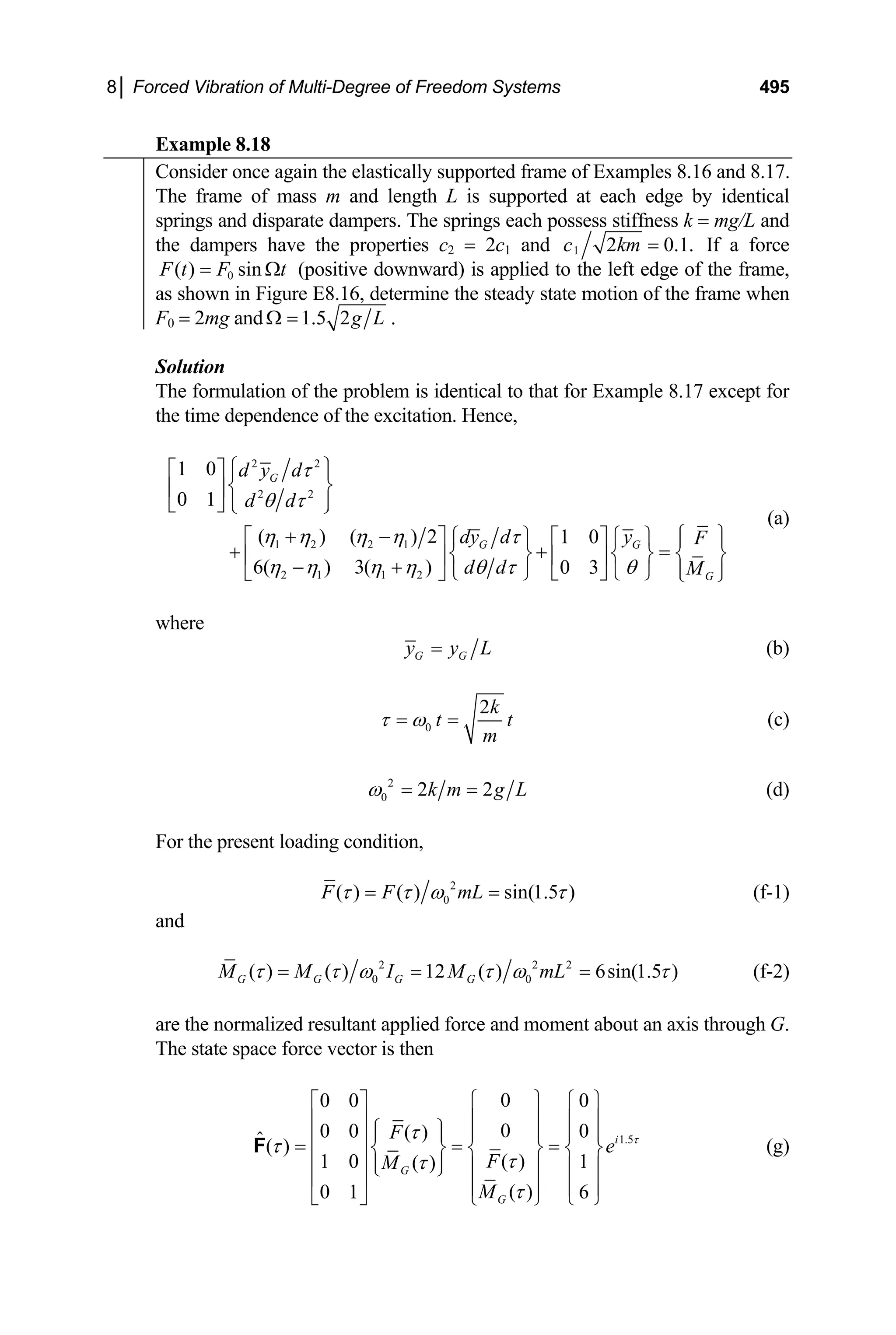
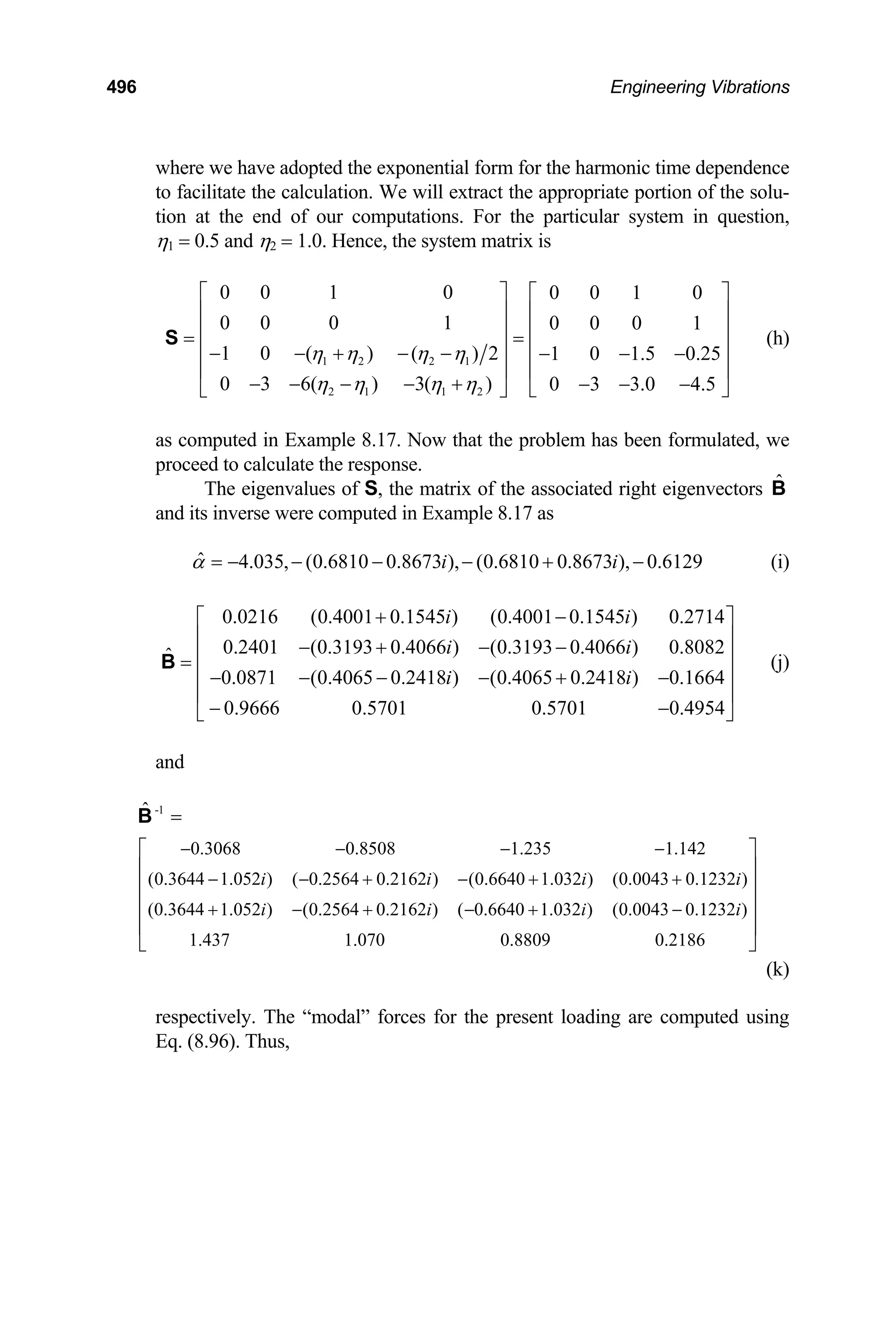
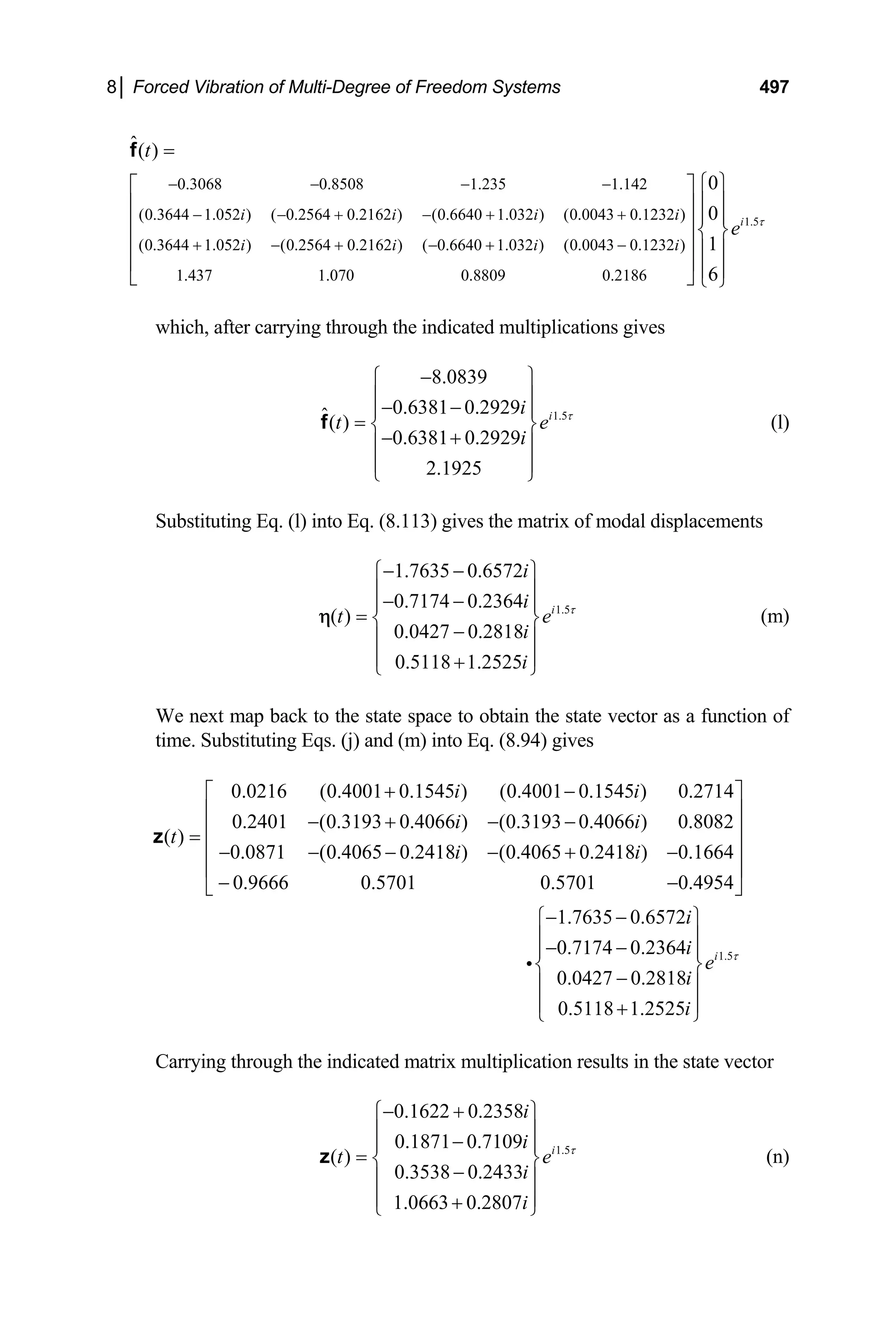
![498 Engineering Vibrations
We now extract the first two rows of the state vector to obtain the displace-
ments
1.5
( ) 0.1622 0.2358
( ) 0.1871 0.7109
G i
y t i
e
t i
τ
θ
− +
⎧ ⎫ ⎧ ⎫
=
⎨ ⎬ ⎨ ⎬
−
⎩ ⎭ ⎩ ⎭
(o)
Expanding Eq. (o) and using Euler’s Formula gives the complex response of
the system,
[ ]
[ ]
( ) 0.1622cos(1.5 ) 0.2358sin(1.5 )
0.2358cos(1.5 ) 0.1622sin(1.5 )
G
y
i
τ τ τ
τ τ
= − +
− +
(p-1)
and
[ ]
[ ]
( ) 0.1871cos(1.5 ) 0.7109sin(1.5 )
0.7109cos(1.5 ) 0.1871sin(1.5 )
i
θ τ τ τ
τ τ
= +
+ − +
(p-2)
Finally, since the excitation is a sine function, the physical response corre-
sponds to the imaginary part of the computed displacements. The steady state
motion of the frame is thus
[ ]
0
( ) 0.2358cos(1.5 ) 0.1622sin(1.5 )
G 0
y t L t t
ω
= − + ω
0t
(q-1)
0
( ) 0.7109cos(1.5 ) 0.1871sin(1.5 )
t t
θ ω
= − + ω (q-2)
The response calculated above compares exactly with the response calculated
in Example 8.16 as, of course, it should.
8.9 CONCLUDING REMARKS
In this chapter we have considered the vibration of systems possessing multiple de-
grees of freedom when they are subjected to a variety of dynamic load conditions.
We studied the behavior of systems with no damping, systems with a special type of
viscous damping known as Rayleigh Damping and systems with general viscous
damping. For the undamped case we began by developing a simple solution for sys-
tems subjected to harmonic loading. The advantage of such an approach was in its
conceptual simplicity. Its implementation, however, requires the inversion of an
N× N matrix, which may be computationally intensive for large systems. In addition,
while this approach provides a convenient mathematical solution, little is gained in
the way of detailing the fundamental mechanisms involved when a system is forced.](https://image.slidesharecdn.com/engineeringvibrations-240713005818-b85f16c0/75/Engineering-Vibrations-Engineering-Vibrations-520-2048.jpg)
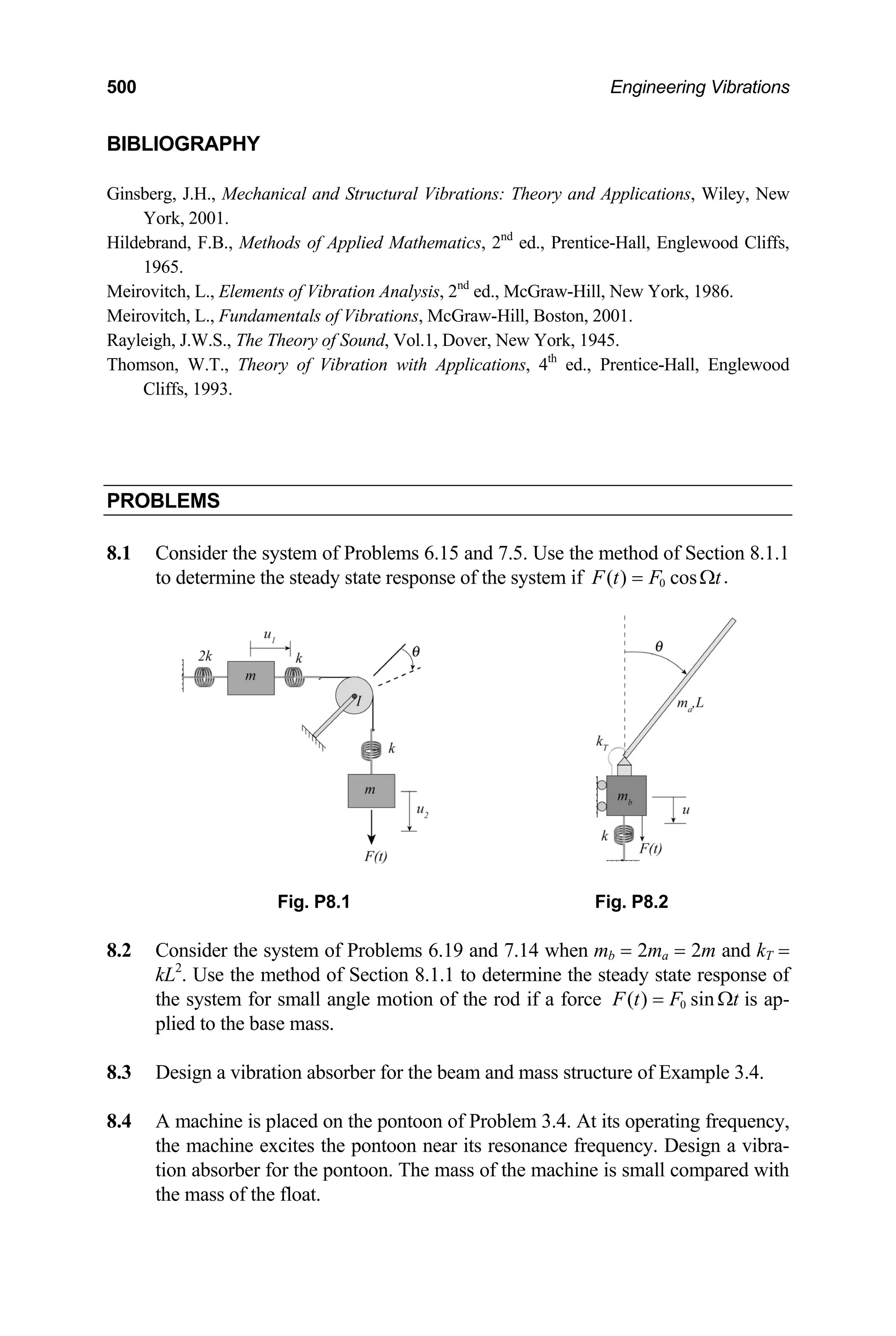
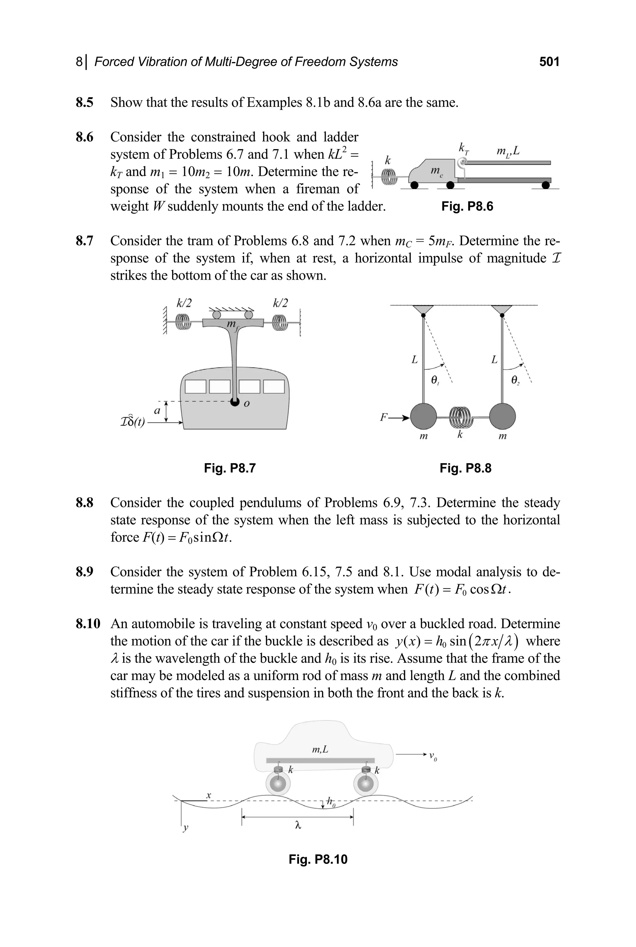
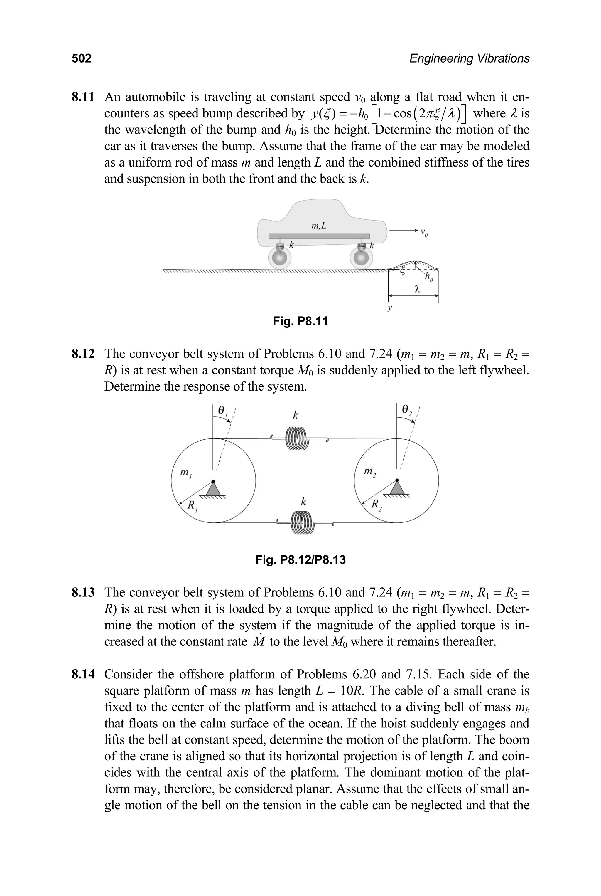
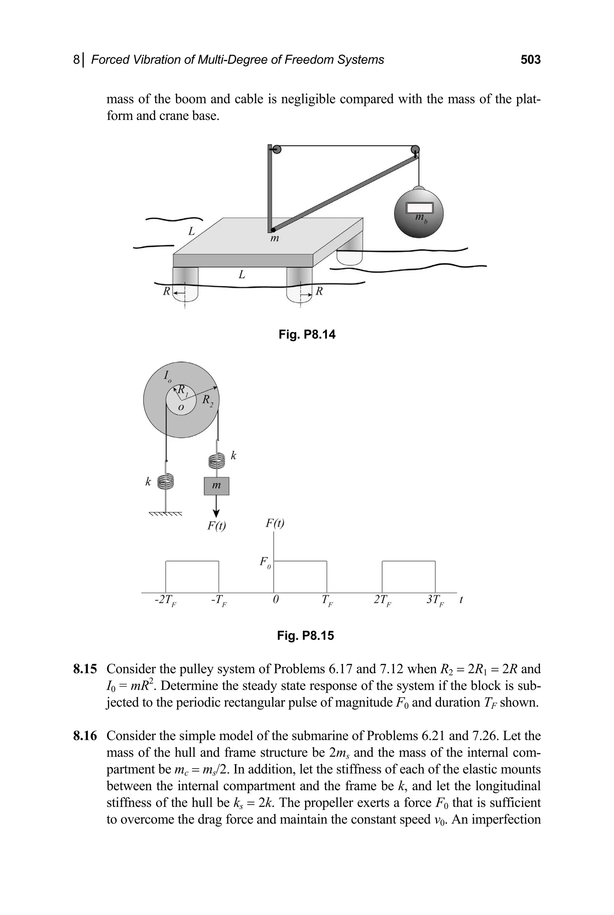
![504 Engineering Vibrations
in the propeller shaft induces a small harmonic perturbation in the thrust of fre-
quency Ω. The actual thrust applied is then of the form 0 0
( ) [1 sin ]
F t F t
ε
= + Ω
where 0 1
ε . If we neglect the corresponding perturbation of the drag force,
determine the response of the submarine.
7.28 where the wings are modeled
as equivalent rigid bodies with torsional springs of stiffness kT at the fuselage
8.18 d 7.25 spins about its axis at the
constant rate ϖ0 as it travels in a fixed orbit at constant speed v0, as shown. The
Fig. P8.16
Fig. P8.17
8.17 Consider the aircraft of Problems 6.31 and
wall, each wing possesses moment of inertia Ic about its respective connection
point and the fuselage of radius R has moment of inertia Io = Ic about its axis.
Let the plane be traveling at constant altitude and speed as it undergoes a ma-
neuver inducing a tight periodic rolling motion of the fuselage with the
sawtooth time history shown. Determine the (perturbed) steady state motion of
the aircraft under these conditions.
The dumbbell satellite of Problems 6.13 an
orbit is maintained such that spin axis is always perpendicular to the surface of
the earth during the orbit. The two compartments are each of mass m and an
elastic access tube of undeformed length L, effective stiffness k and negligible](https://image.slidesharecdn.com/engineeringvibrations-240713005818-b85f16c0/75/Engineering-Vibrations-Engineering-Vibrations-526-2048.jpg)
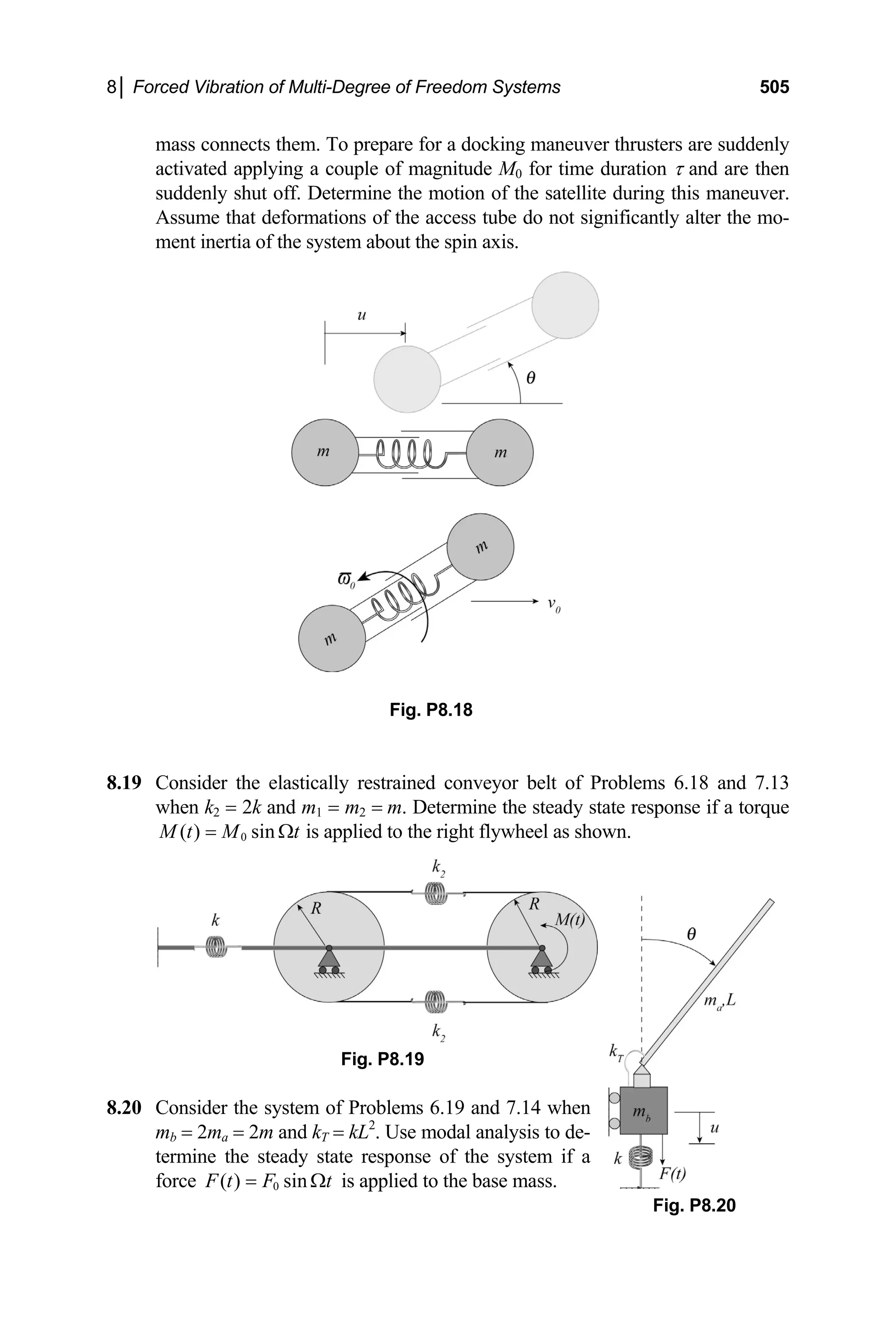
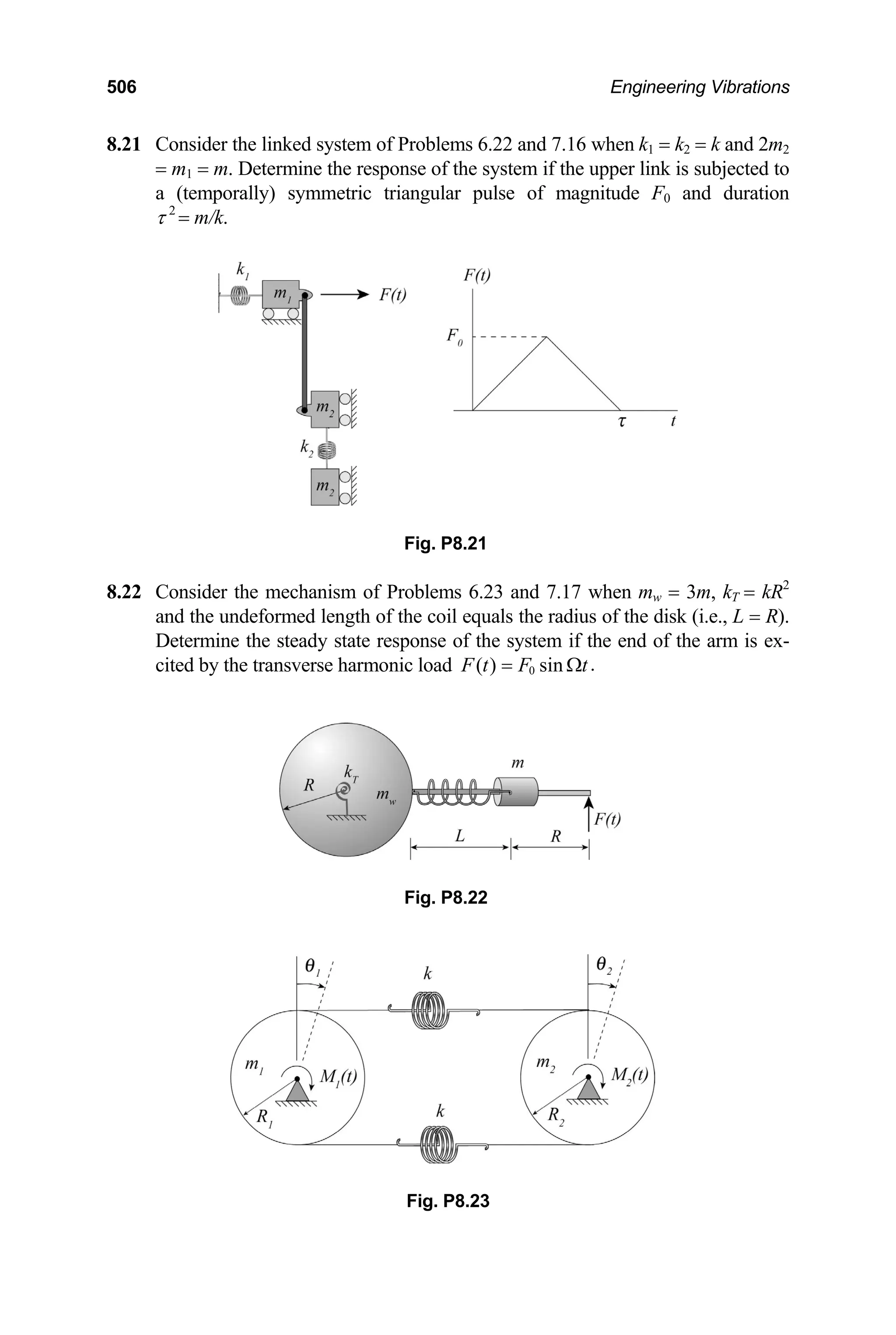
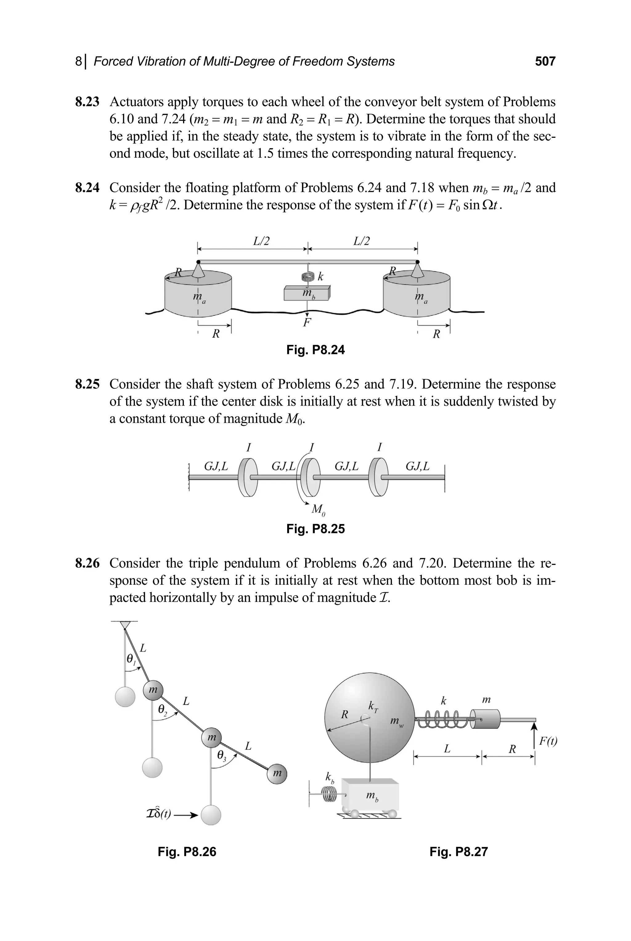
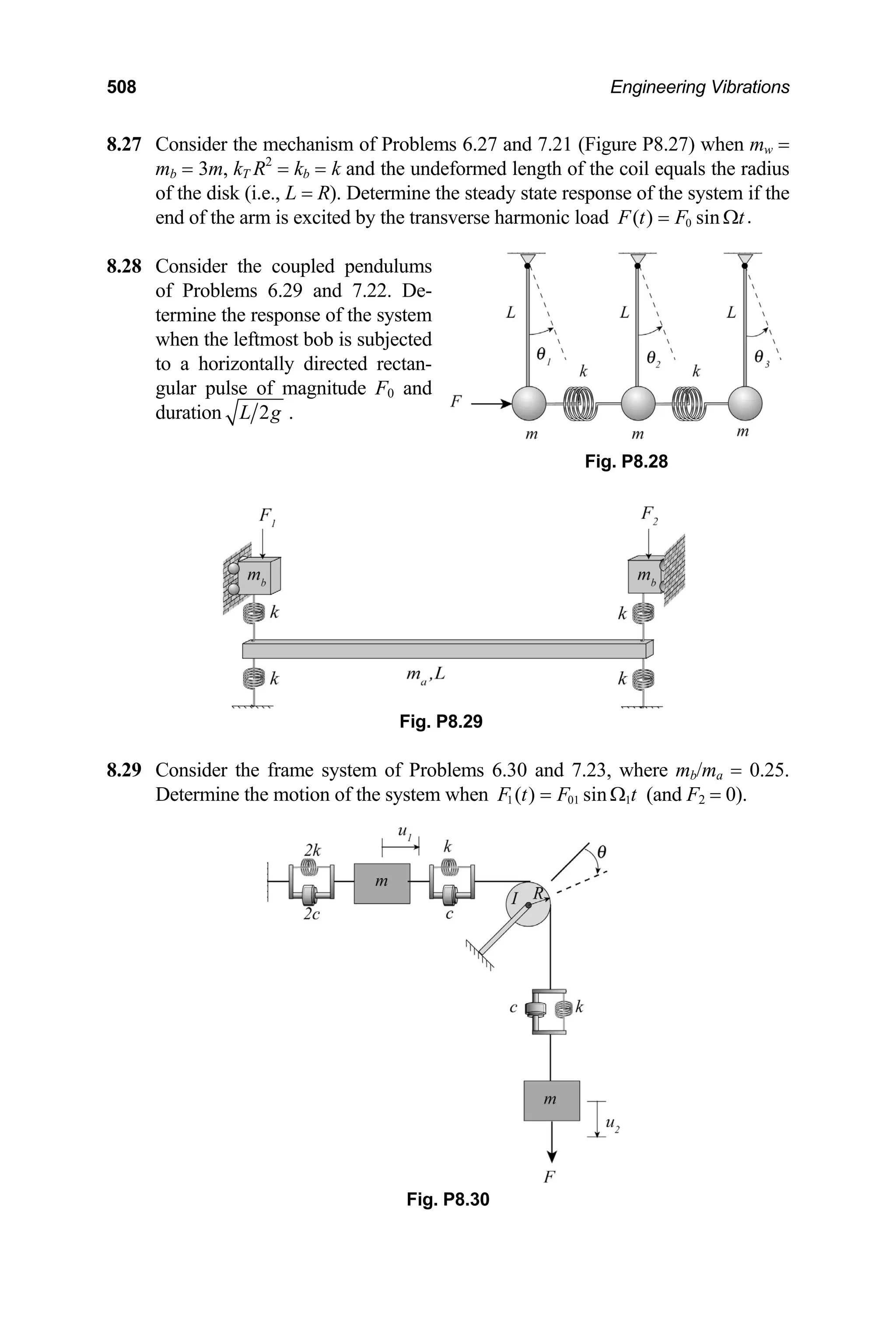
![8│ Forced Vibration of Multi-Degree of Freedom Systems 509
8.30 Consider the system of Problems 6.36 and 7.40 (c2
/km = 0.04, I = 2mR2
). De-
termine the steady state response of the system if 0 .
( ) cos
F t F t
= Ω
mine the response of the two-mass three-spring three-damper system of
8.31 Deter
Problem 7.37 when the left mass is subjected to the pulse ( ) ( ).
F t t
δ
= I
.32 Consider the system of Problem 6.32 and 7.38
8
when mb = 2ma = 2m, kT = kL2
and c2
/km =
0.04. Determine the steady state response of
the system if a force 0
( ) sin
F t F t
= Ω is ap-
plied to the base mass.
Fig. P8.32
.33 Repeat Problem 8.16, this time taking into account the effect of the perturbation
.34 Consider the simple model of the submarine of Problem 6.37, where the mass
8
on the drag force where the corresponding coefficient is cd = c.
8
of the internal compartment is mc, the mass of the hull and frame structure is
ms = 2mc, the stiffness of each of the elastic mounts between the internal com-
partment and the hull frame is k, the damping factor for each of the mounts is
0.1 ,
c
c km
= the longitudinal stiffness of the hull is ks = 2k and the effective
r of the hull is c
damping facto s = 2c. The propeller exerts a force F0 that is suf-
ficient to overcome the drag force and maintain the constant speed v0. An im-
perfection in the propeller shaft induces a small harmonic perturbation in the
thrust of frequency Ω. The actual thrust applied is then of the form
0 0
( ) [1 sin ]
F t F t
ε
= + Ω where 0 1
ε . If we neglect the corresponding pertur-
, determin response of the submarine.
bation of the drag force e the
Fig. P8.34](https://image.slidesharecdn.com/engineeringvibrations-240713005818-b85f16c0/75/Engineering-Vibrations-Engineering-Vibrations-531-2048.jpg)
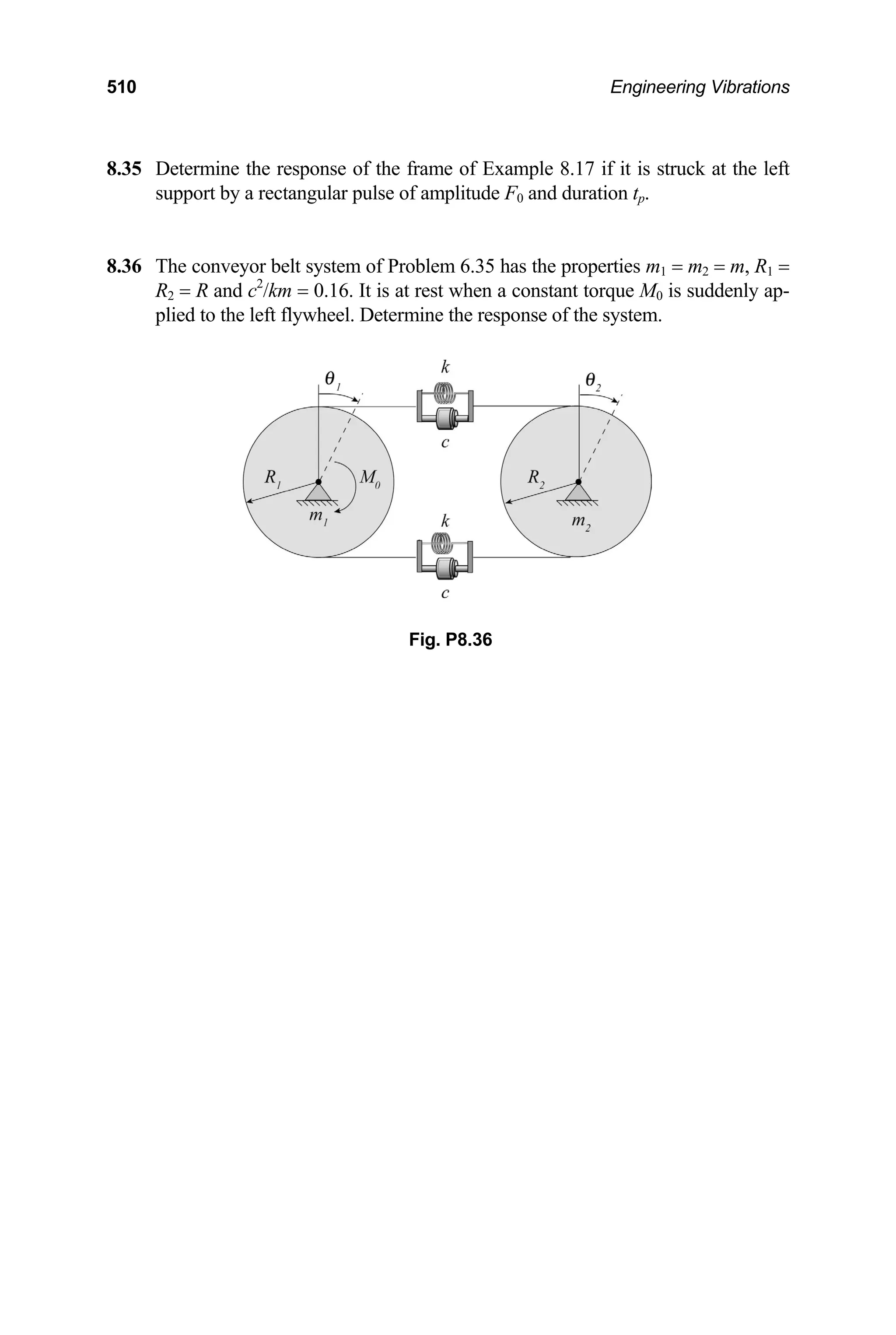
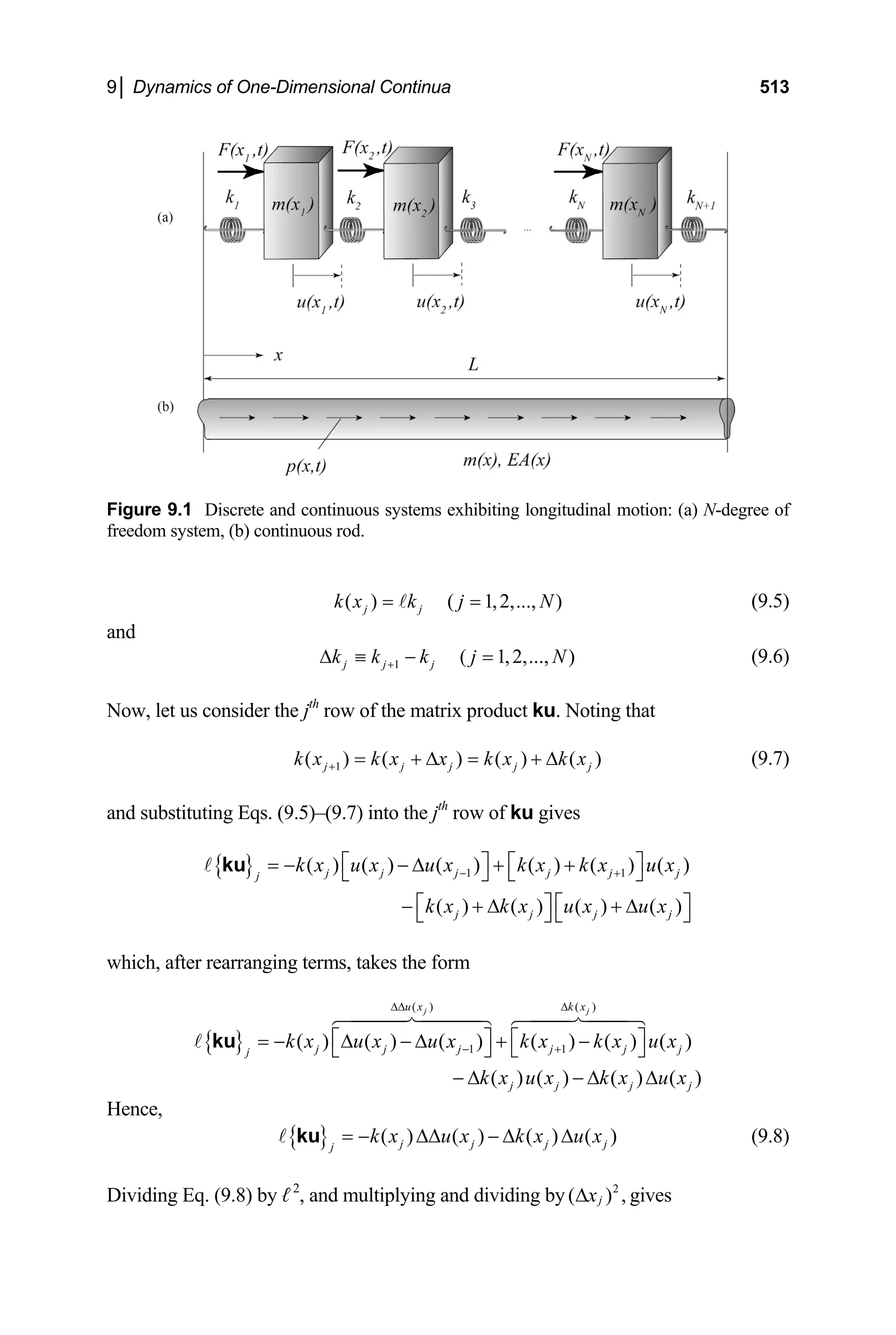
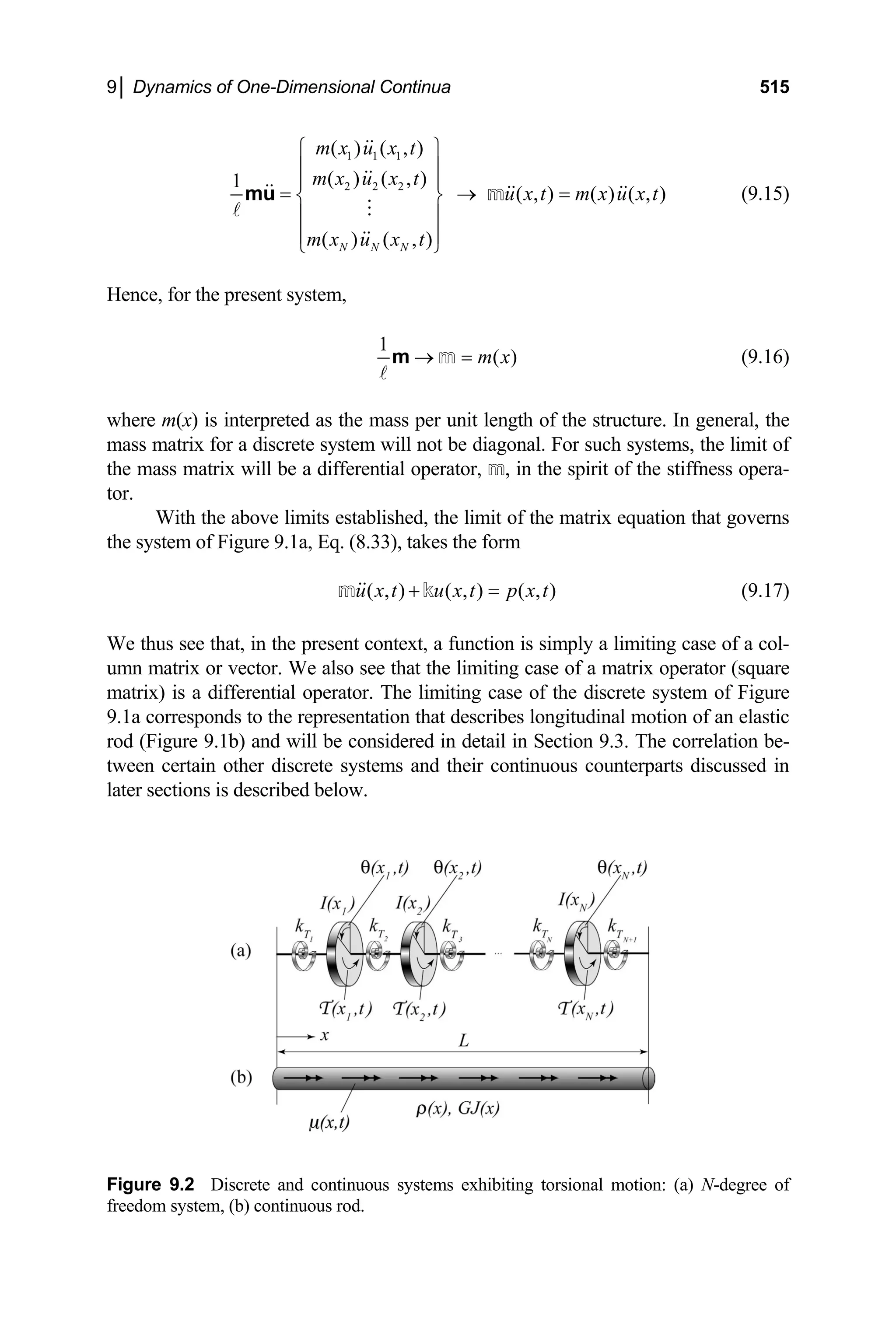
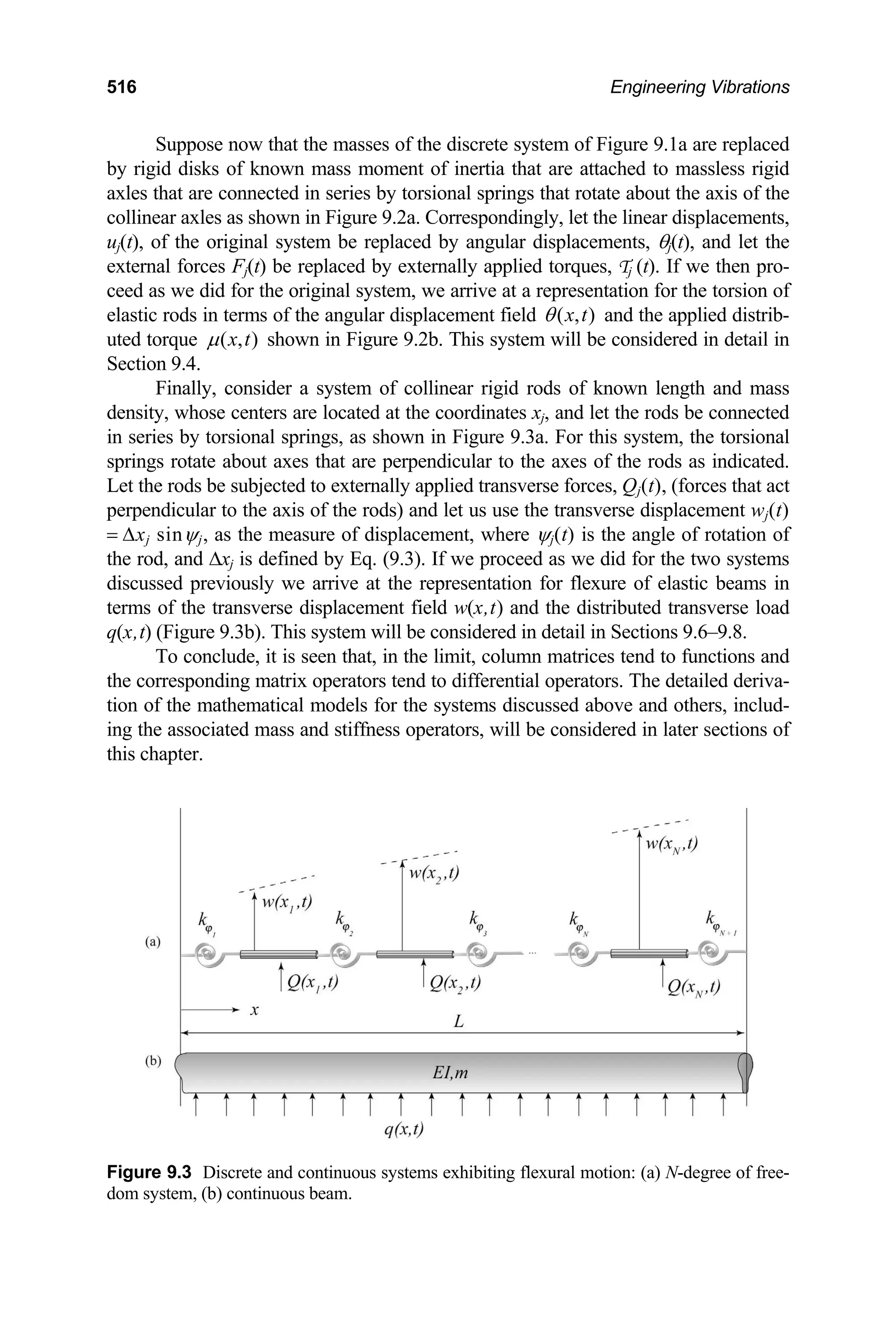
![518 Engineering Vibrations
( ) ( )
{ } { }
0 0
, ( ) ( ) sin 2 sin 2
sin 2 ( ) sin 2 ( )
0 0 0
2 ( ) 2 ( )
L L
f g f x g x dx n x L p x L
n p n p
n p L n p L
π π
π π
π π
= =
− +
= − = − =
− +
∫ ∫ dx
Thus, on [0, L].
f g
⊥
Note that the given functions would be orthogonal on the domain [−L, L]
as well. Compare the above functions with the functions used as the basis for
conventional Fourier Series (Section 3.6). It may be seen that a Fourier Series is
an expansion in terms of a set of mutually orthogonal functions.
The Weighted Scalar Product
It follows from Eq. (7.25), that the weighted scalar product of two vectors u and v
with respect to a matrix m is given by
1 1 1 1
, ( ) ( ) ( ,
N N N N
l lj j l lj j
l j l j
u t v t u x t v x t
= = = =
= = =
∑∑ ∑∑
m
u v u mv
T
m m
) ( , ) (9.21)
It is seen, upon incorporating Eq. (9.13) into Eq. (9.21), that the weighted scalar
product with respect to a diagonal mass matrix simplifies to the form
1
, ( , ) ( ) (
N
j j j
j
u x t m x v x t
=
= ∑
m
u v , ) (9.22)
Taking the limit as and
N → ∞ , j
x dx
∆ → gives the scalar product of the two
functions u(x,t) and v(x,t) with respect to the weight function m(x). Hence,
0
, ( , ) ( ) ( ,
L
m
u v u x t m x v x t dx
=
∫ ) (9.23)
If the weighted scalar product vanishes, the functions u(x,t) and v(x,t) are said to be
orthogonal with respect to the weight function m(x). Stated mathematically,
if , 0 then ( , ) ( , )
m m
u v u x t v x t
= ⊥ (9.24)
The weighted scalar product of two vectors, u and v, with respect to the stiff-
ness matrix k is defined as discussed in Section 7.3.1. Hence,](https://image.slidesharecdn.com/engineeringvibrations-240713005818-b85f16c0/75/Engineering-Vibrations-Engineering-Vibrations-540-2048.jpg)
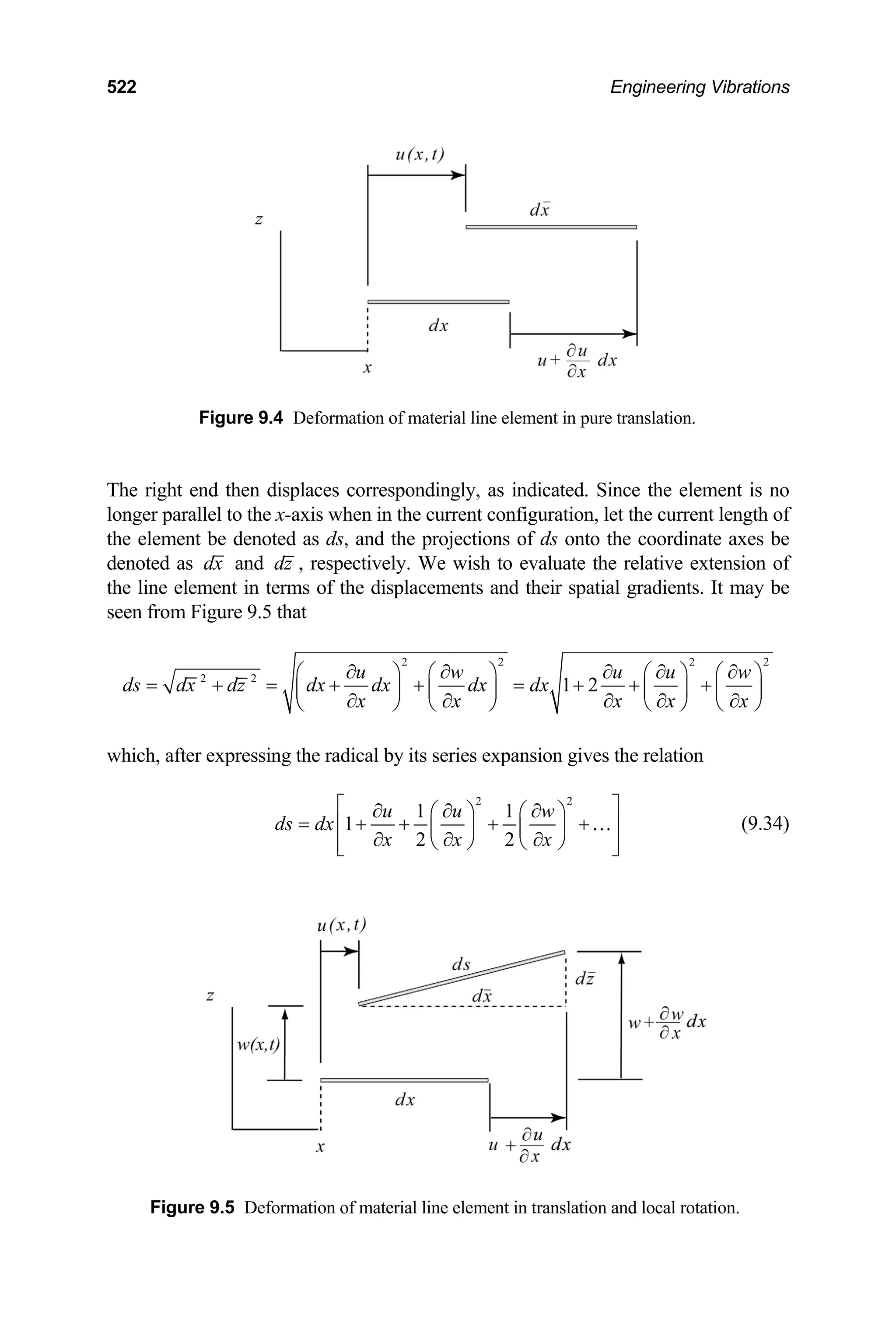
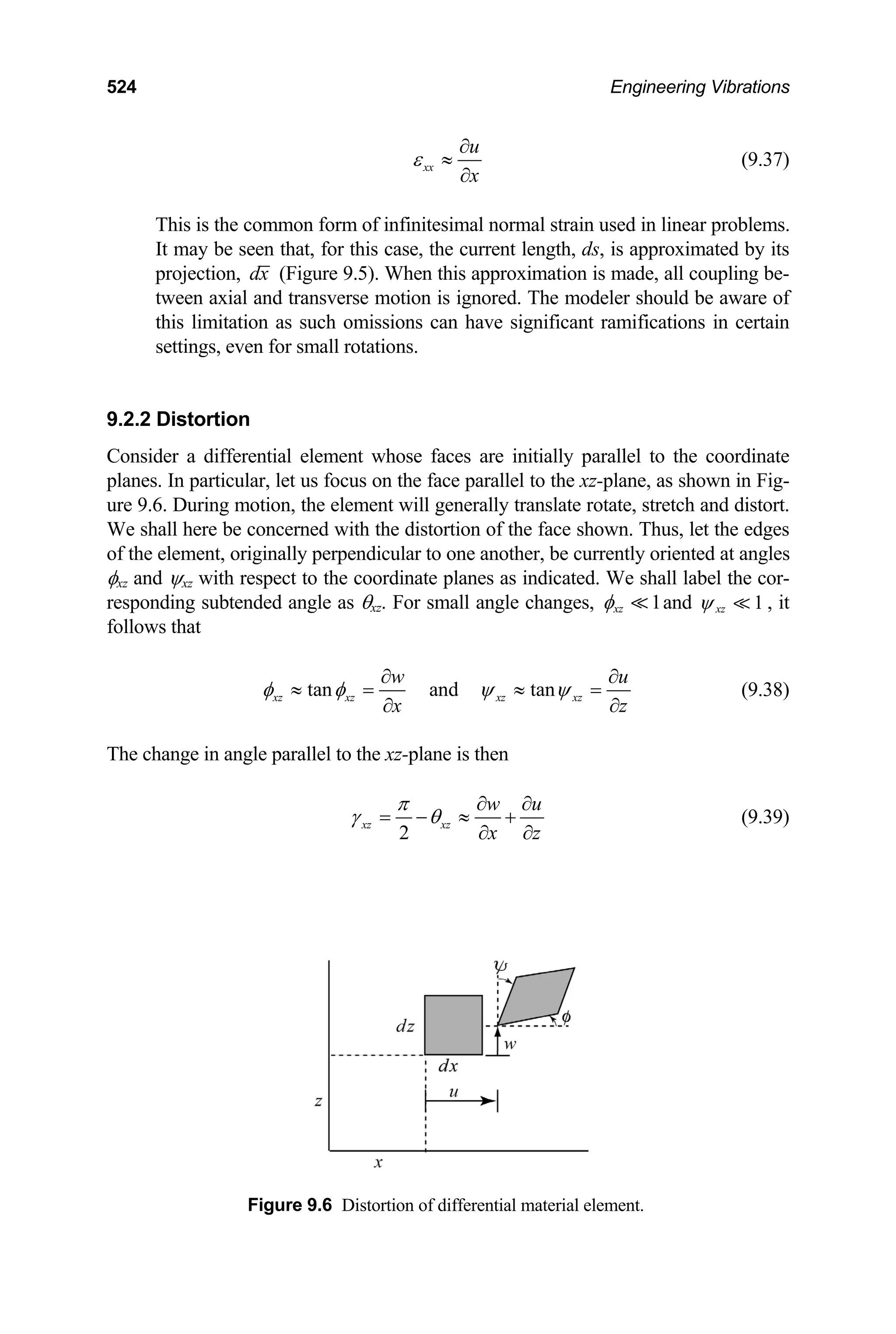
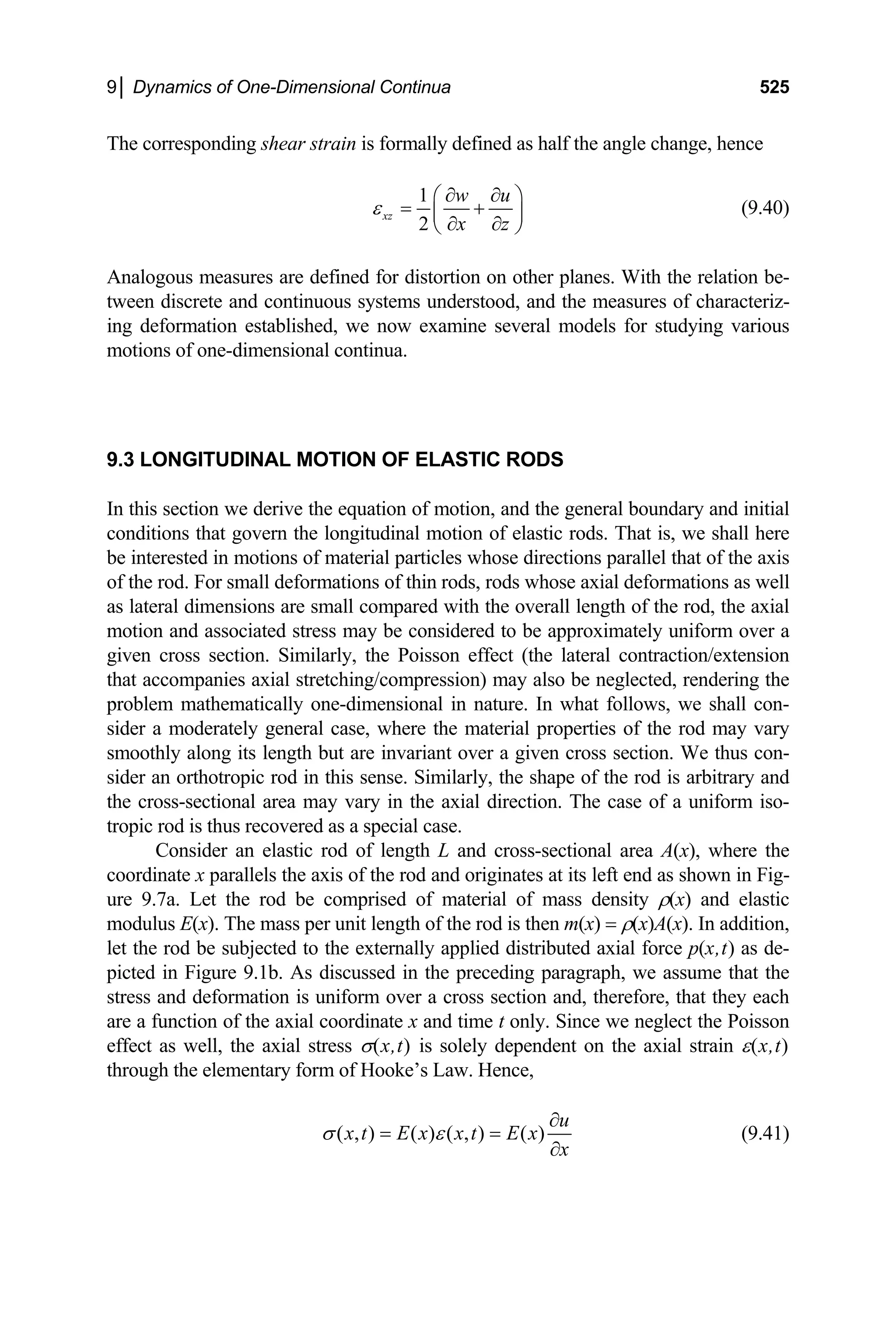
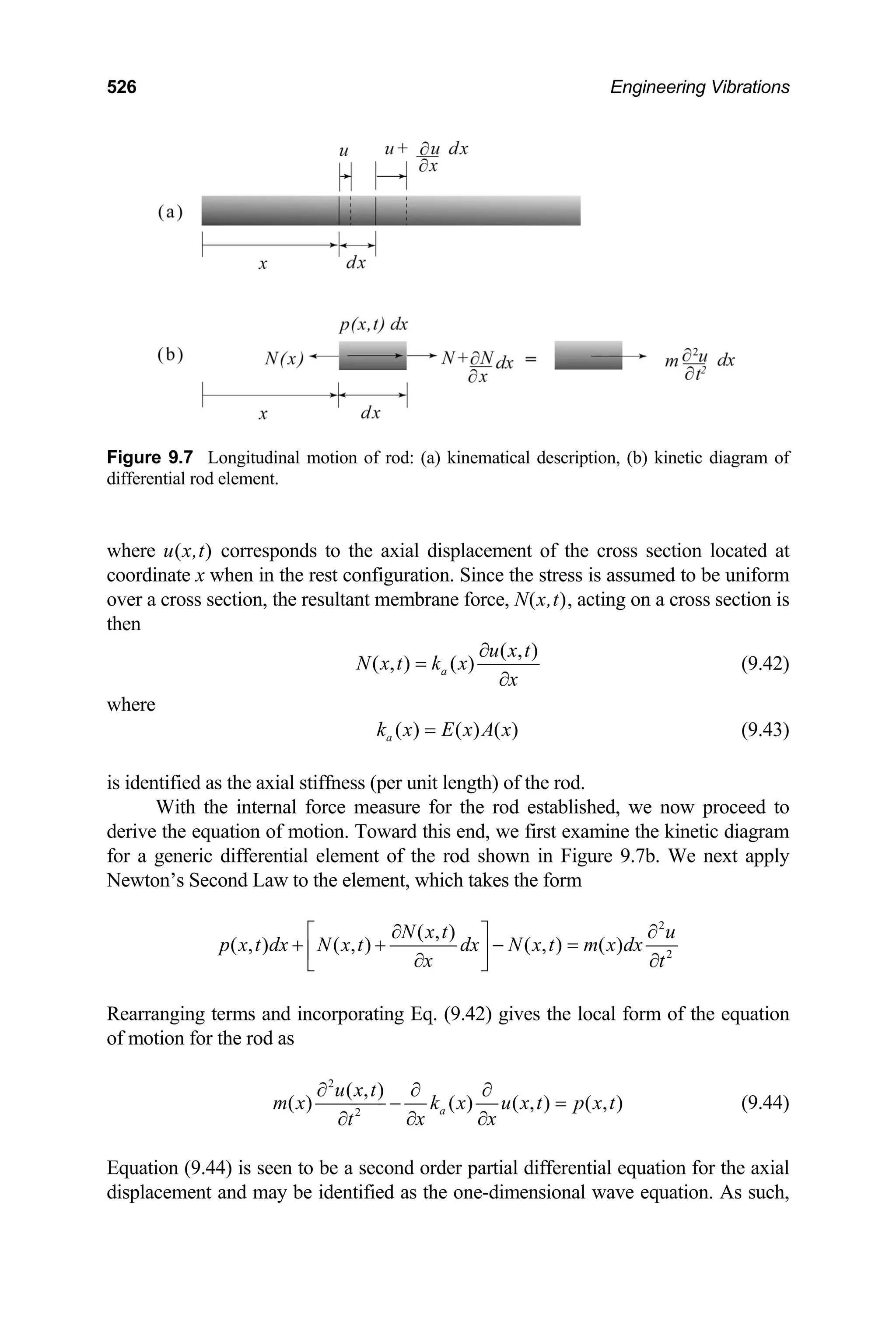
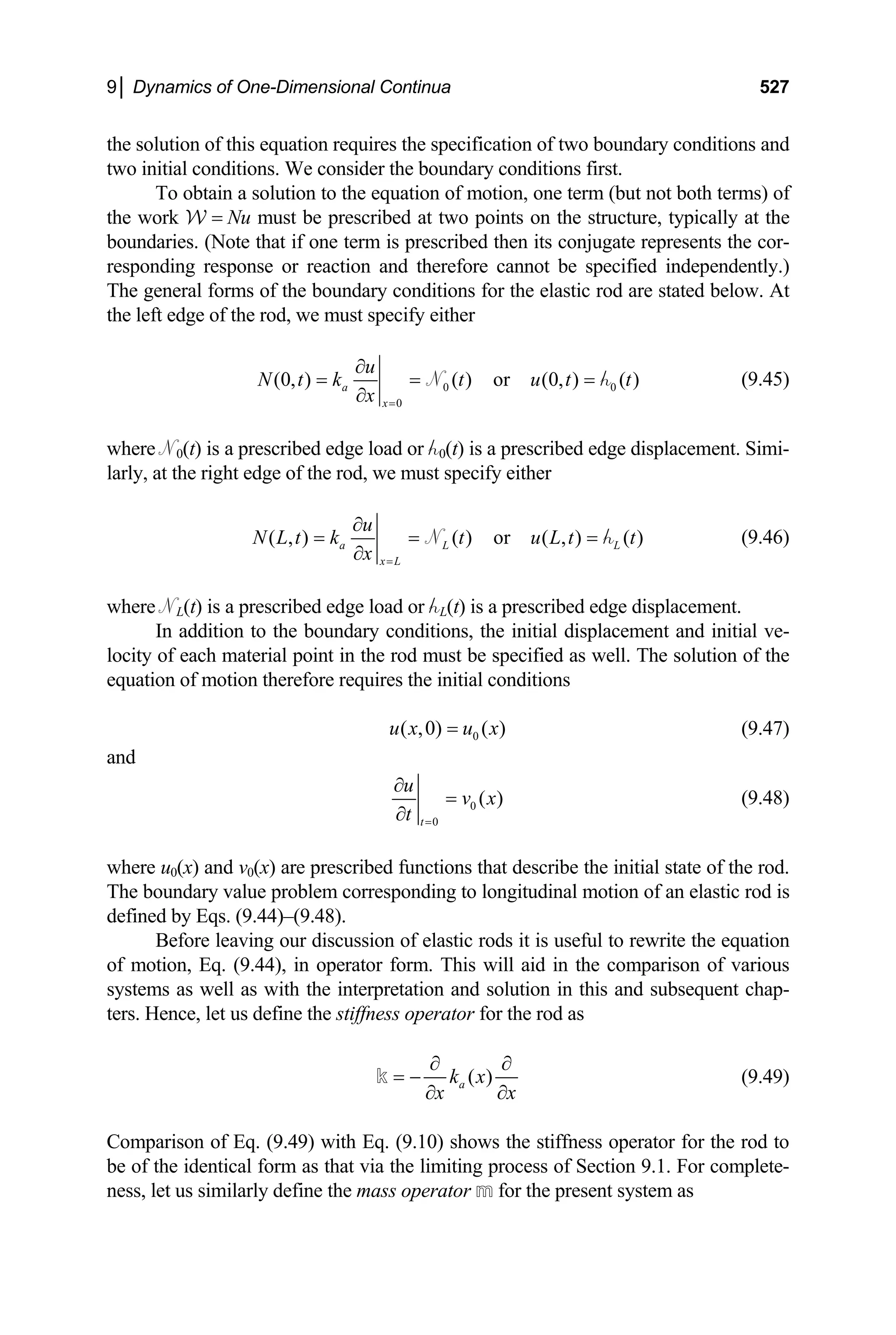
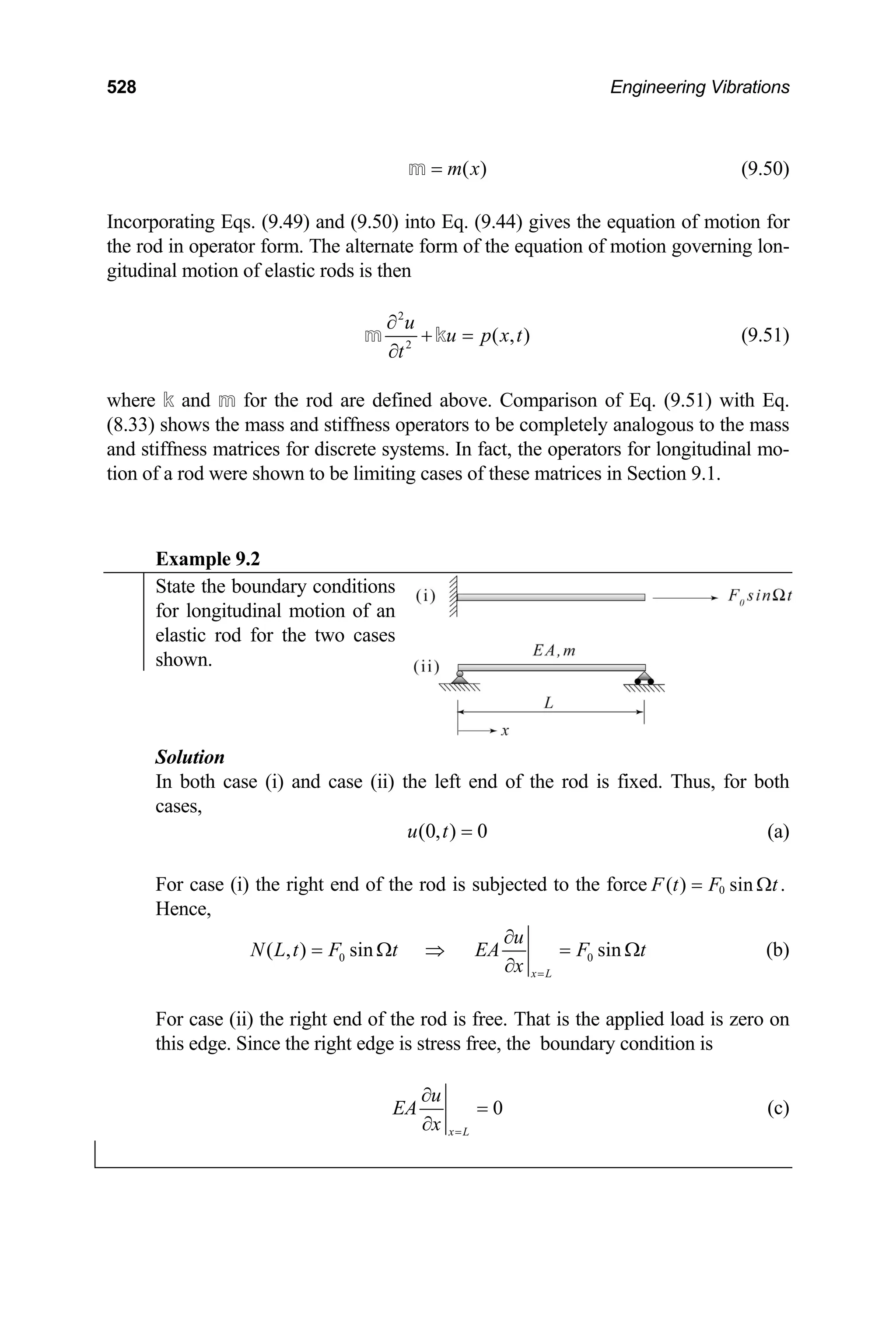
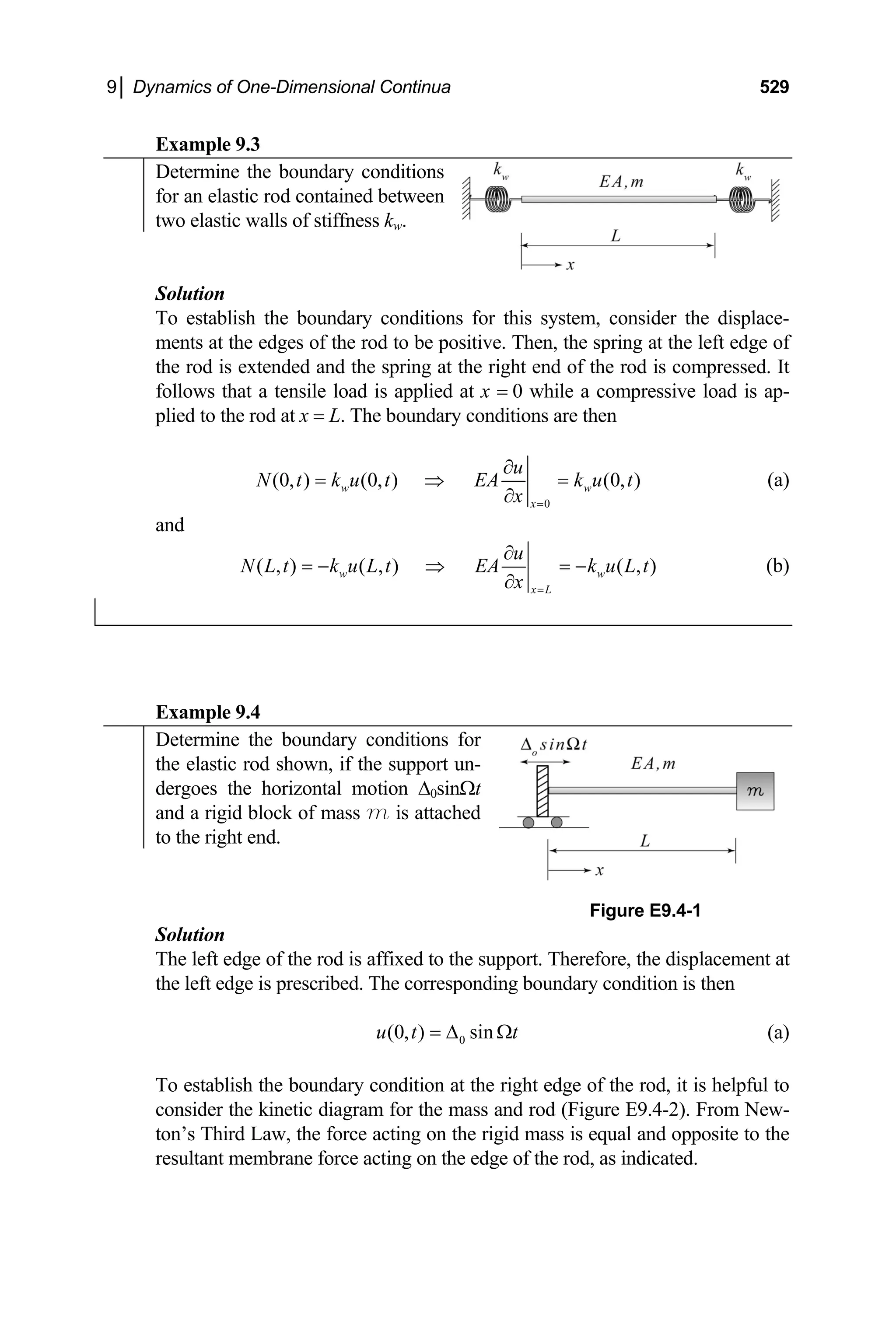
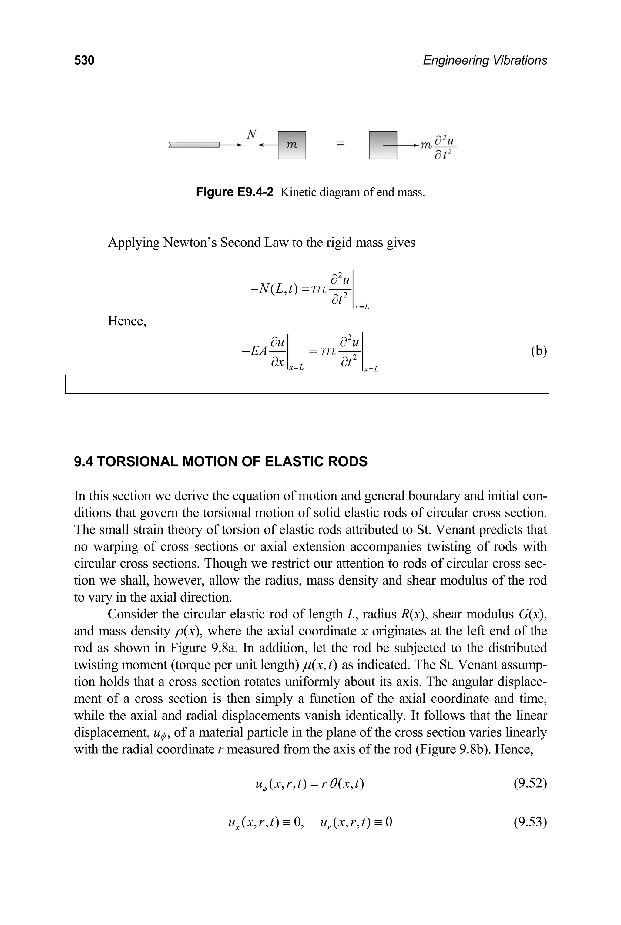
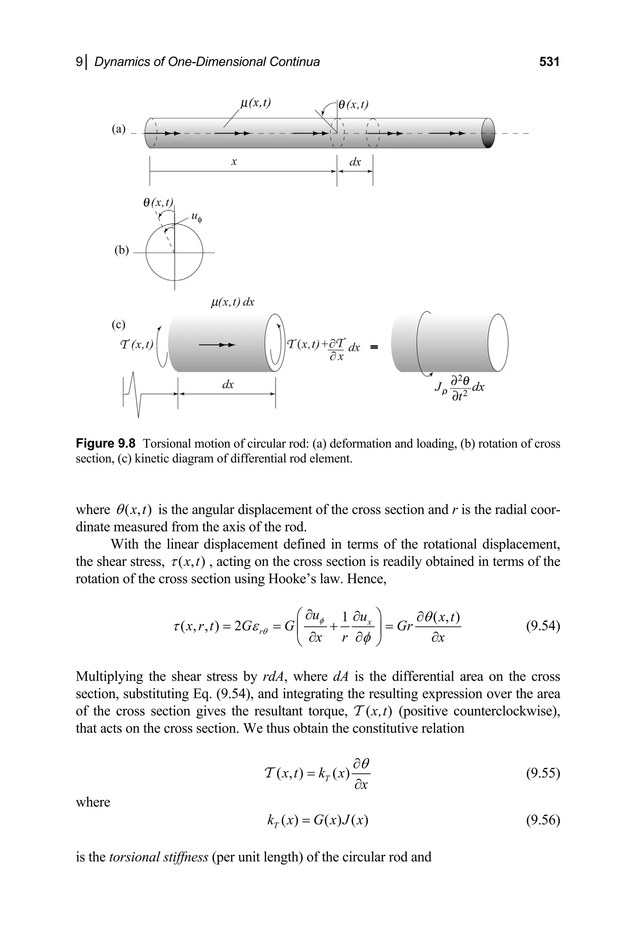
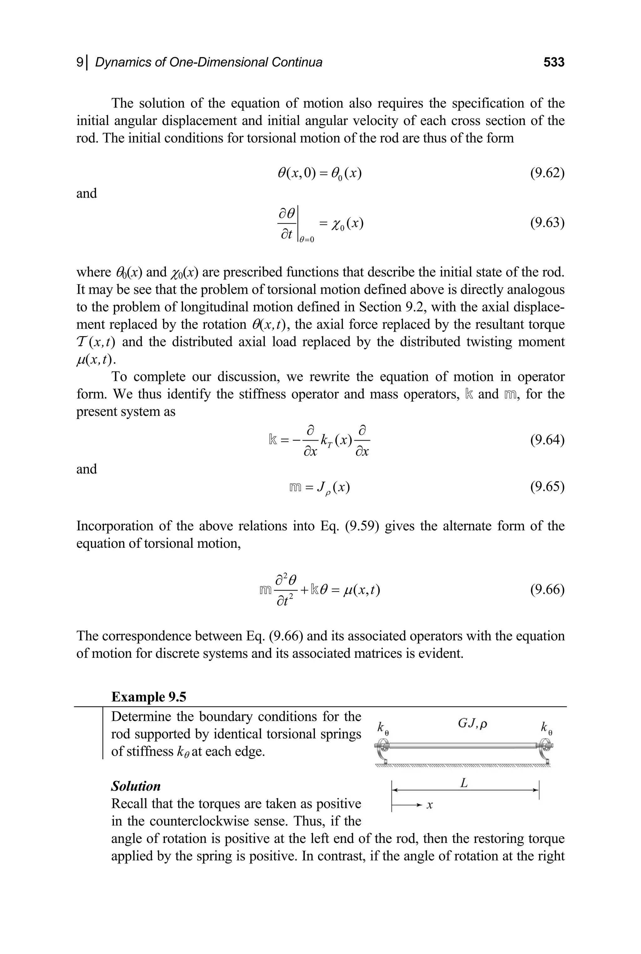
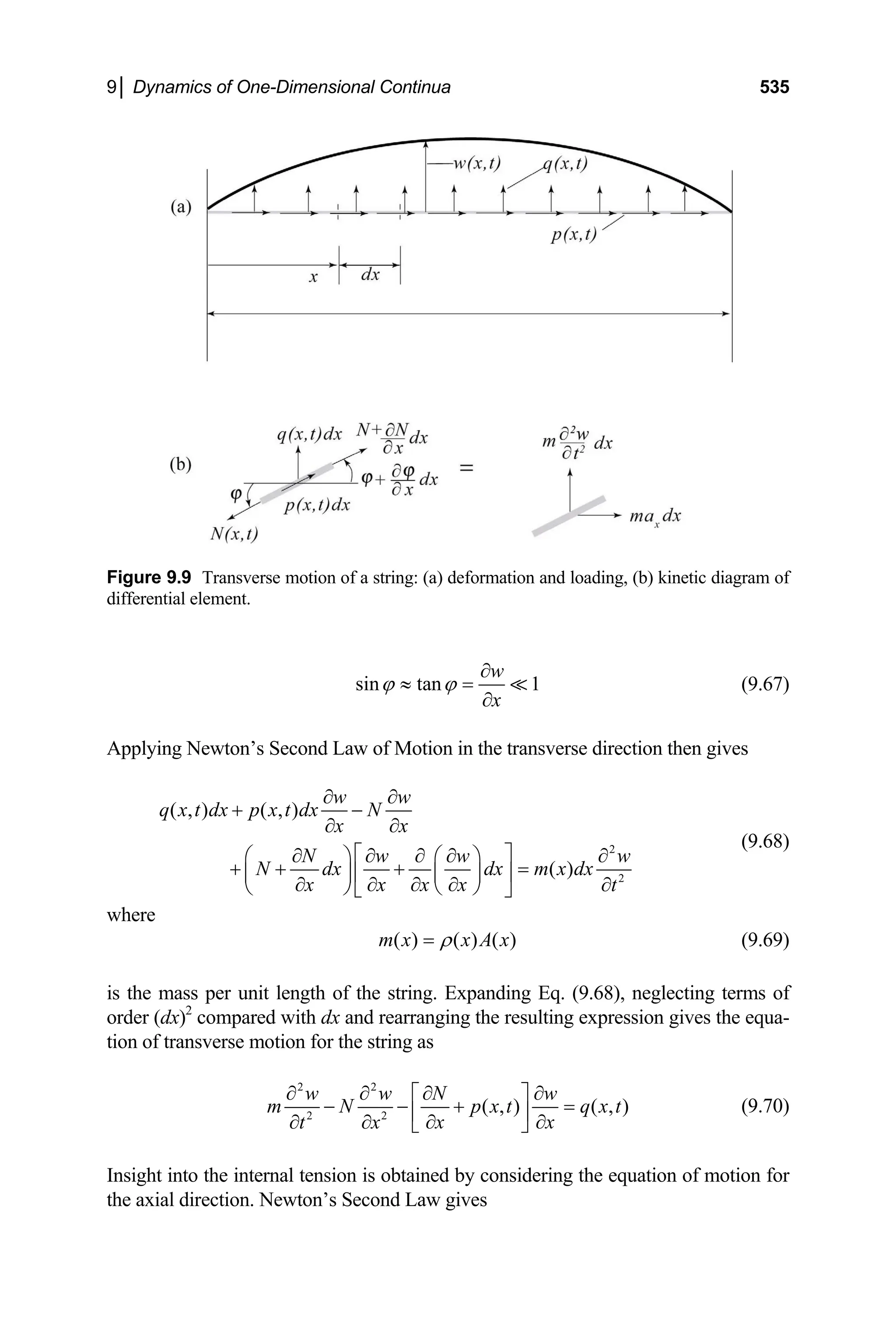
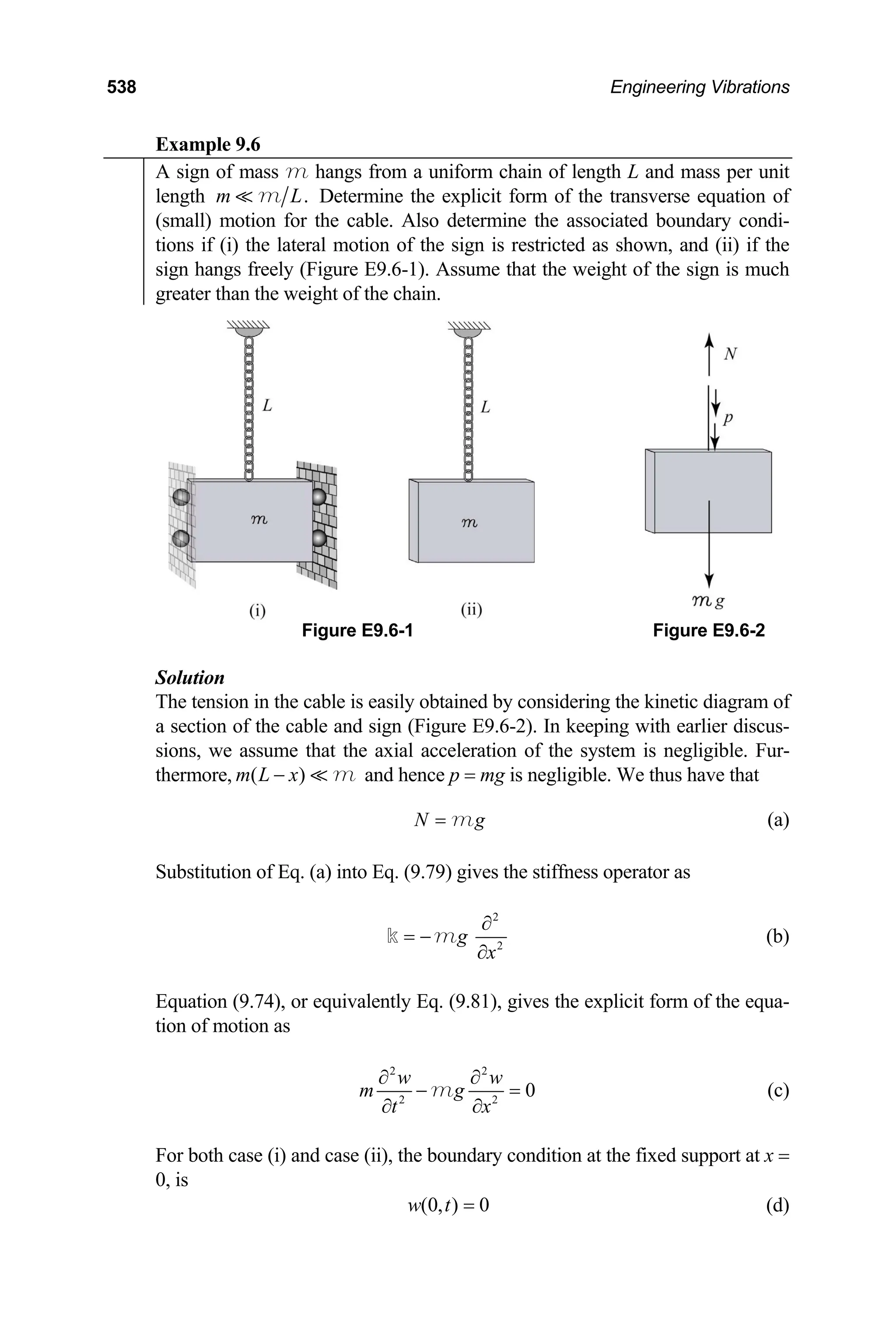
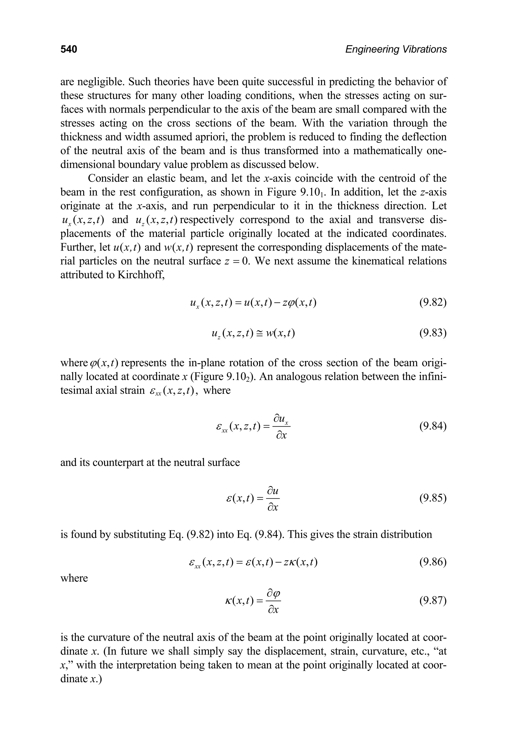
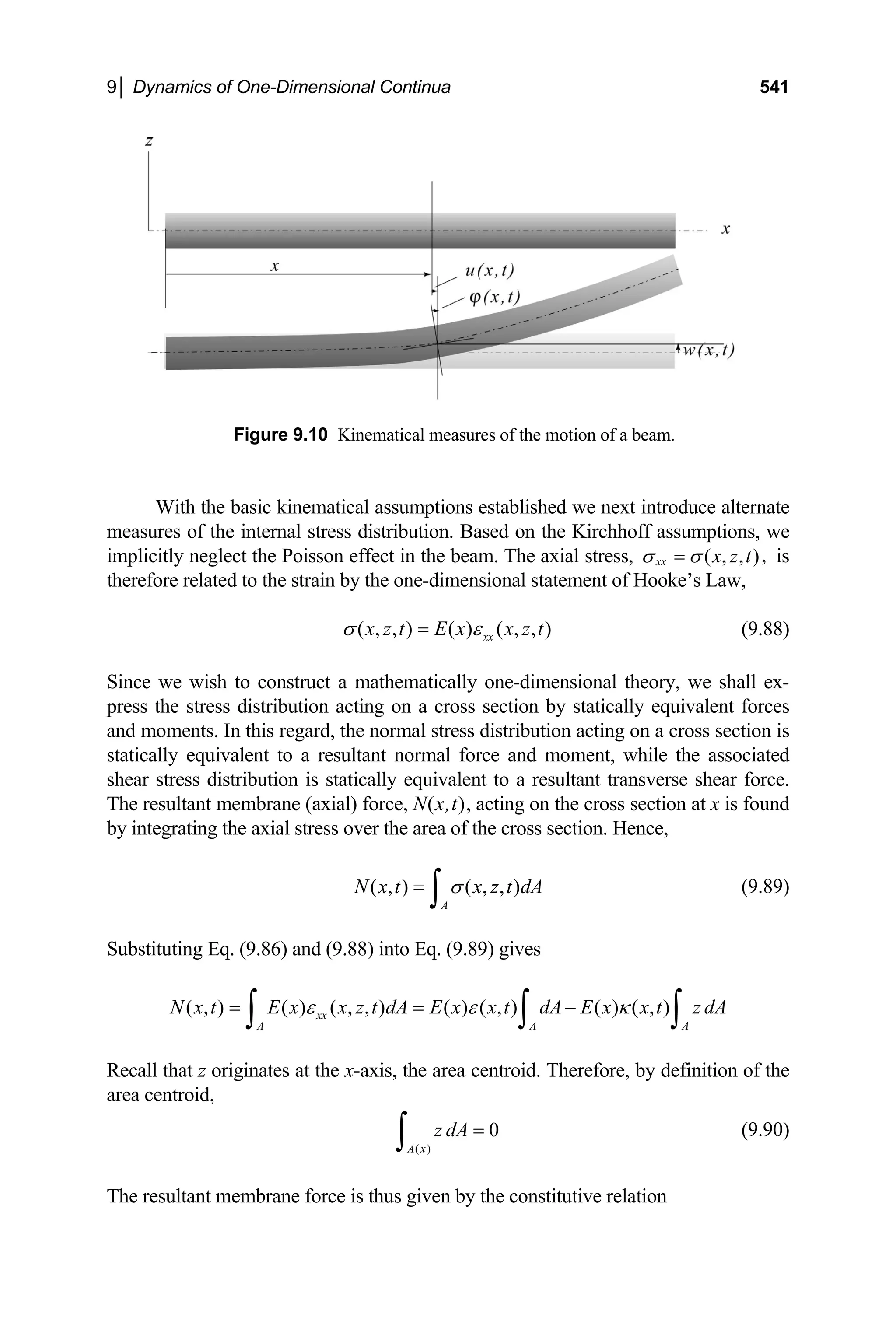
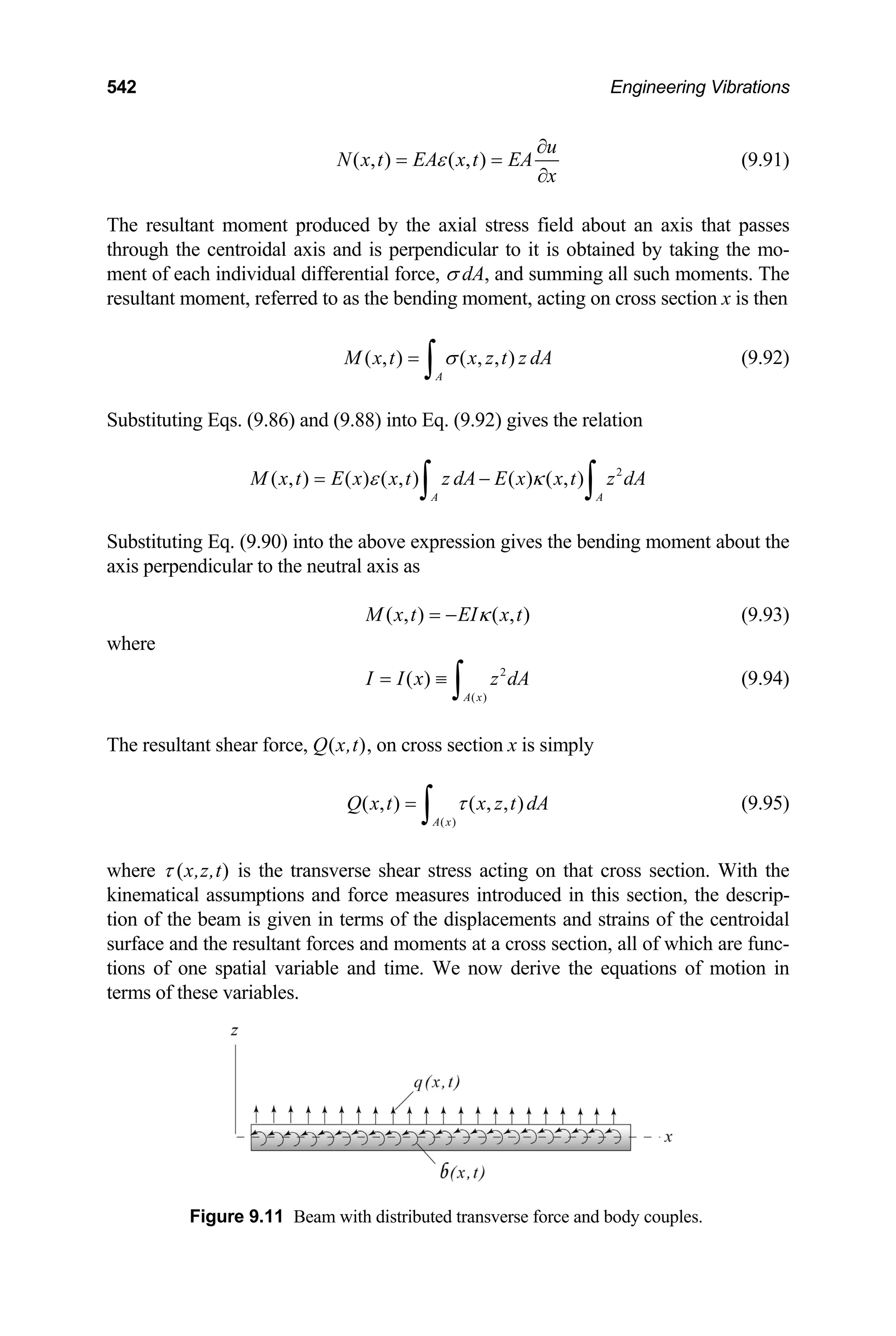
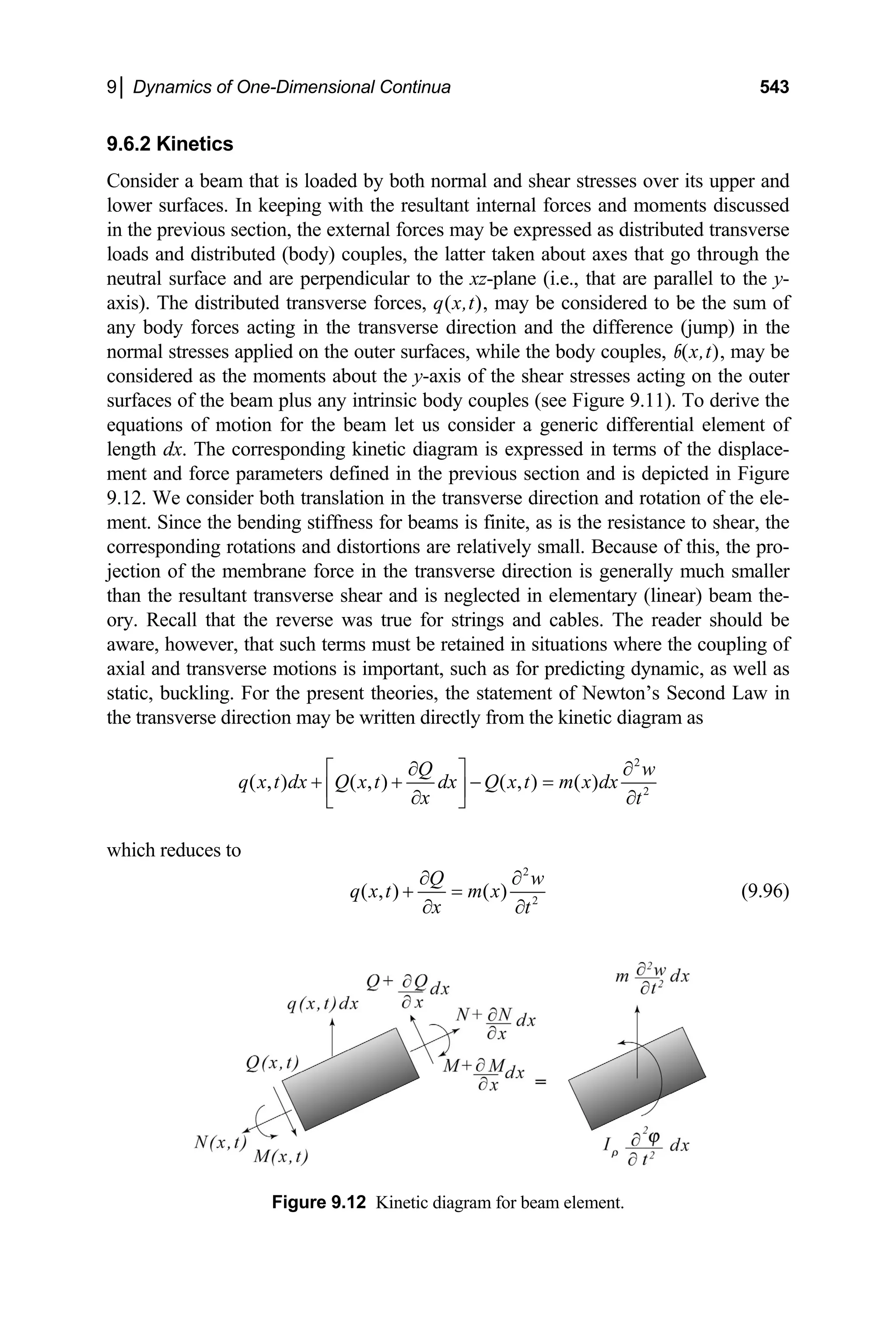
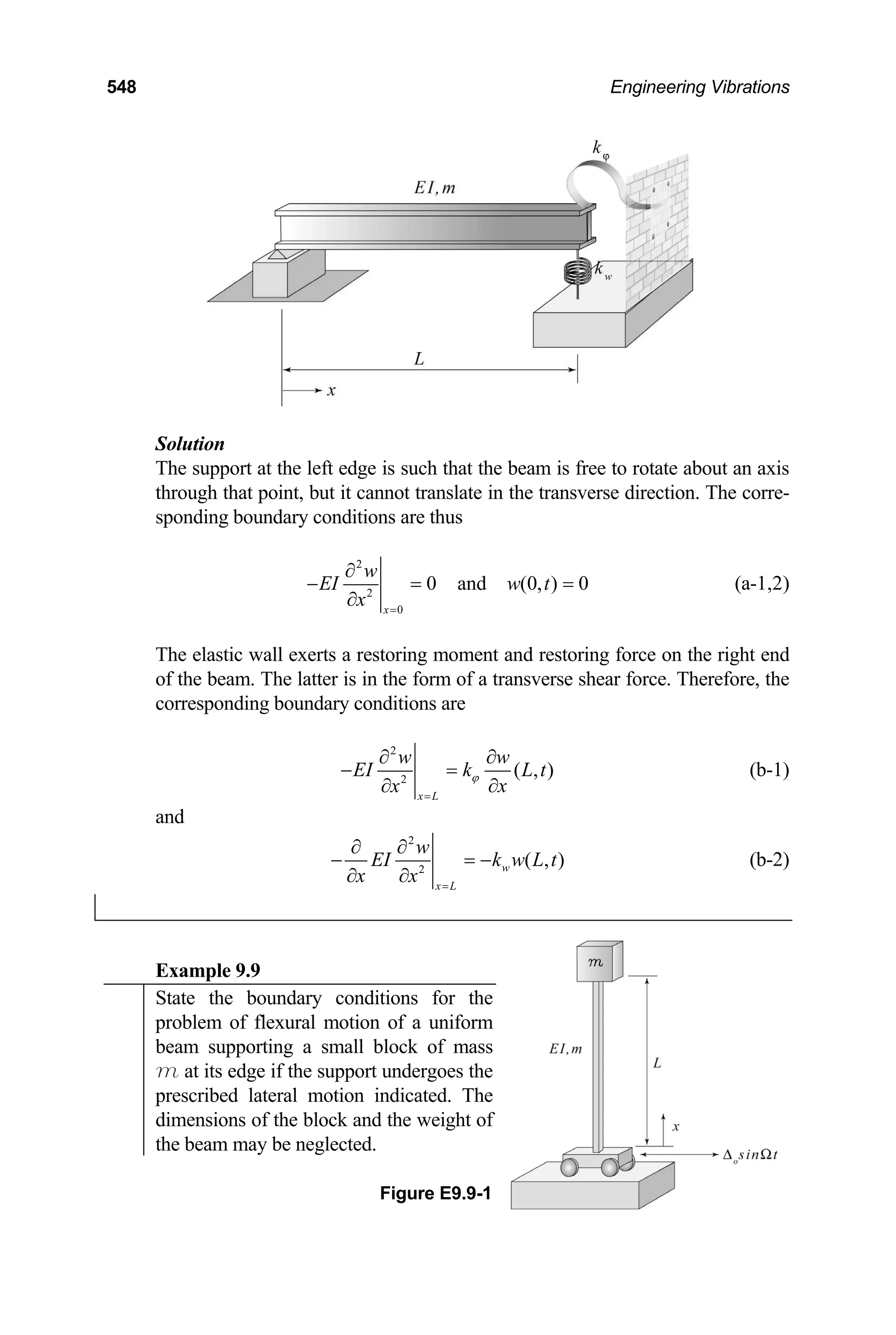
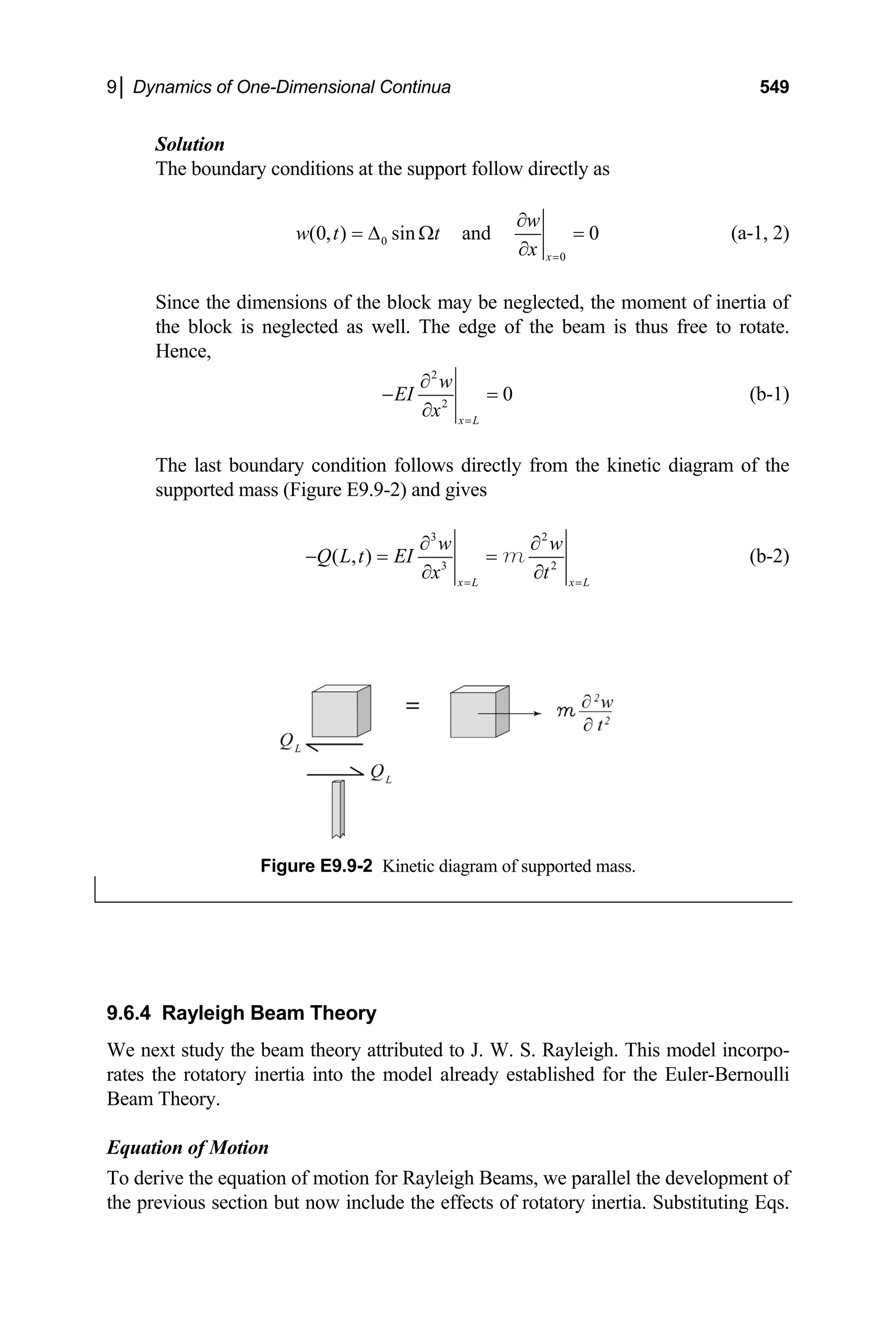
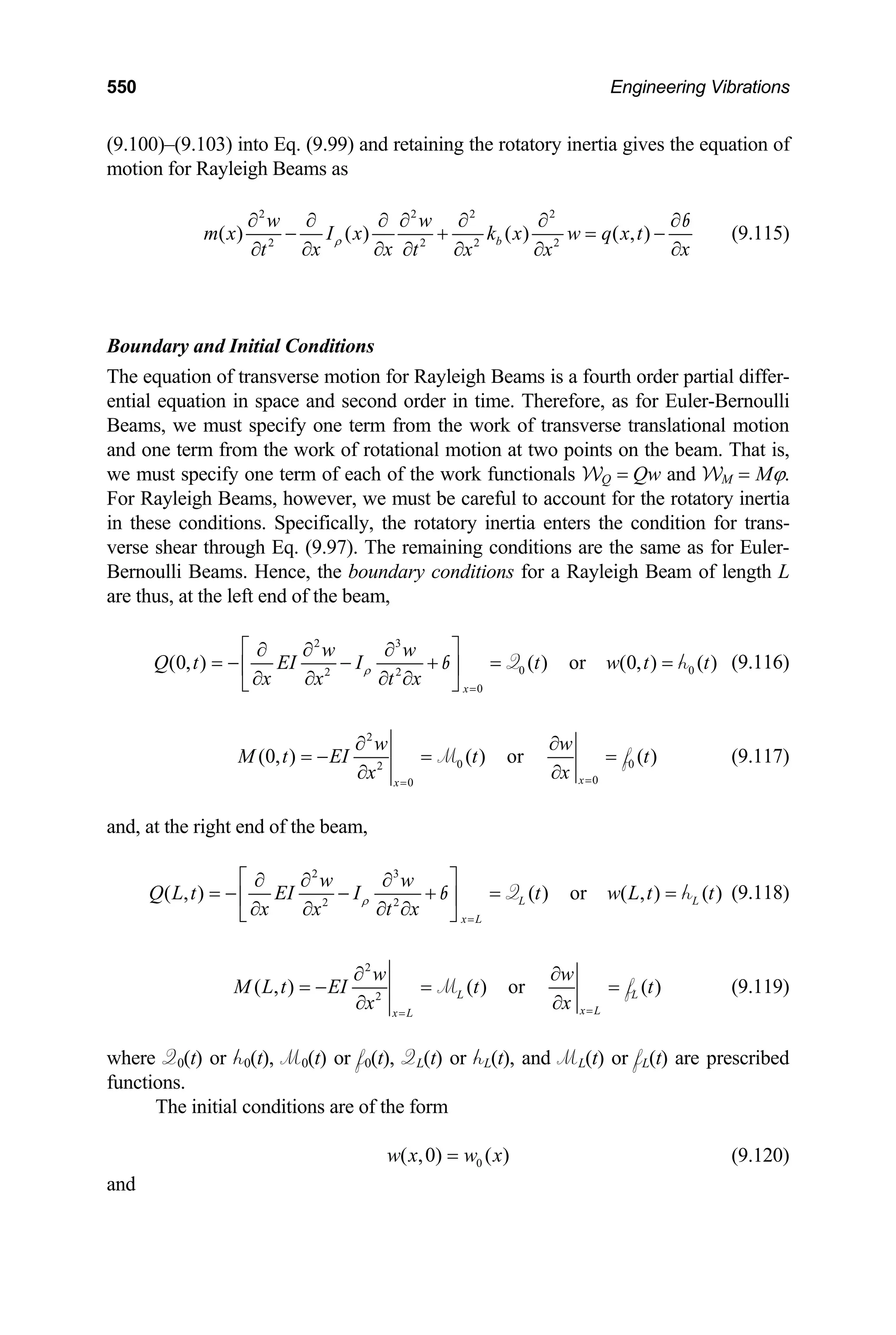
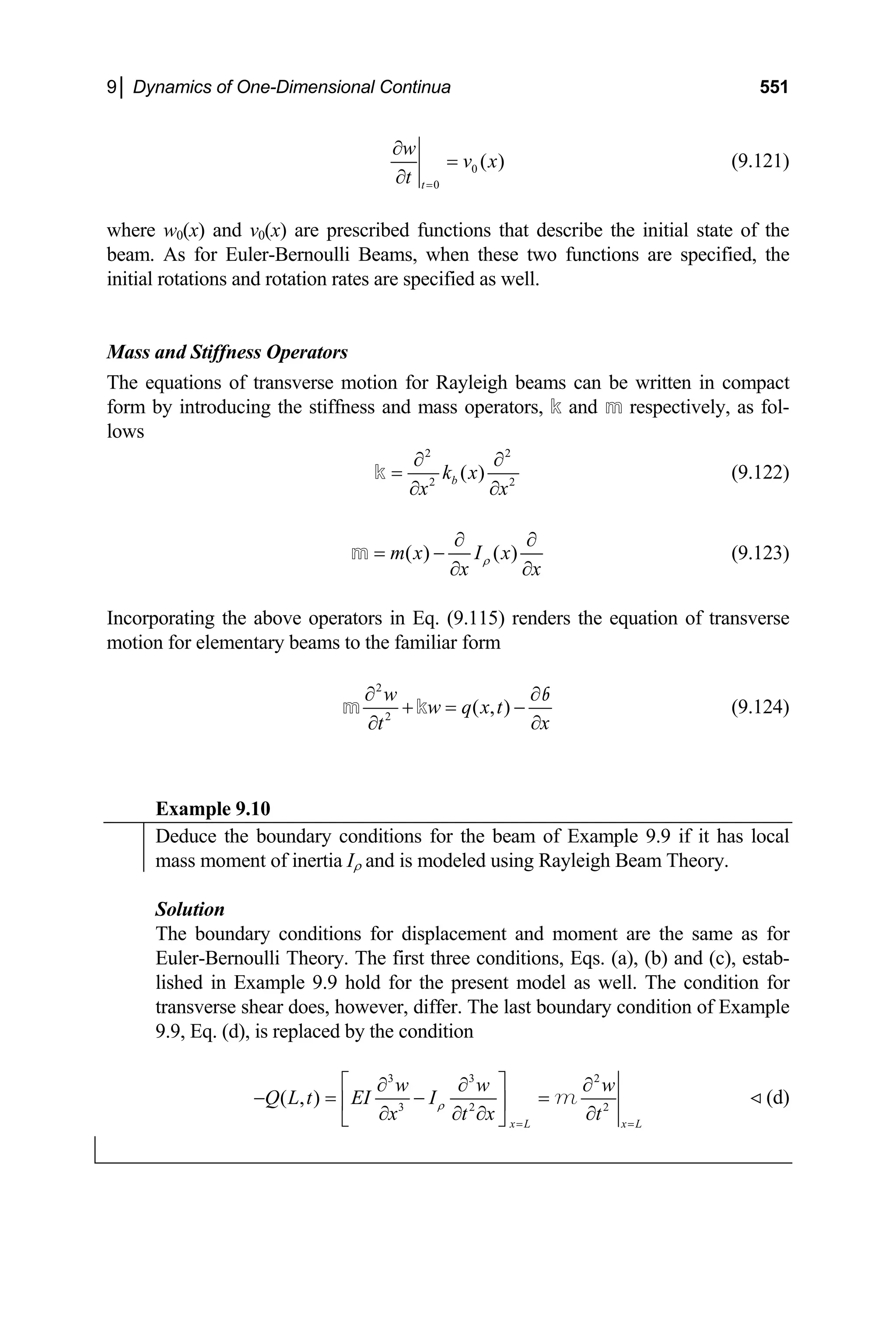
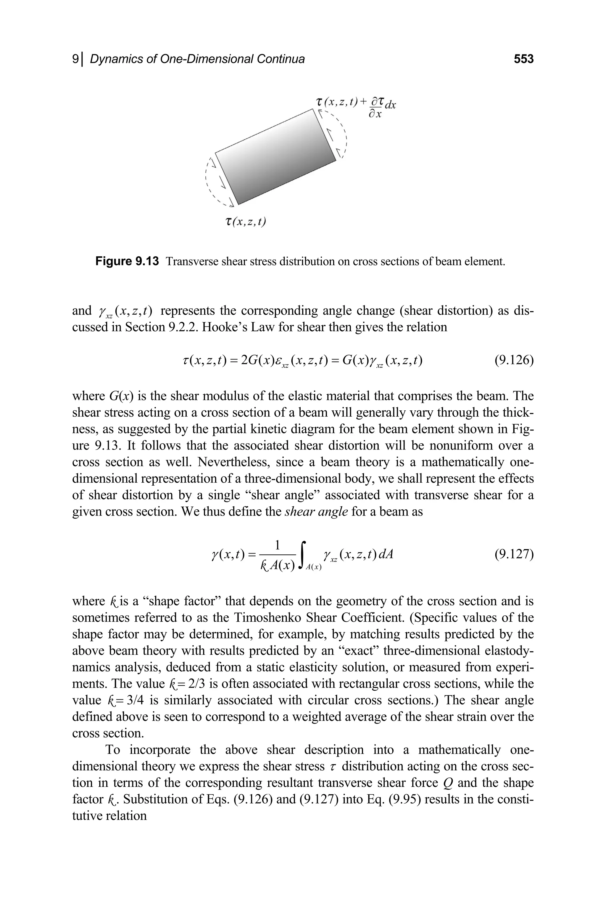
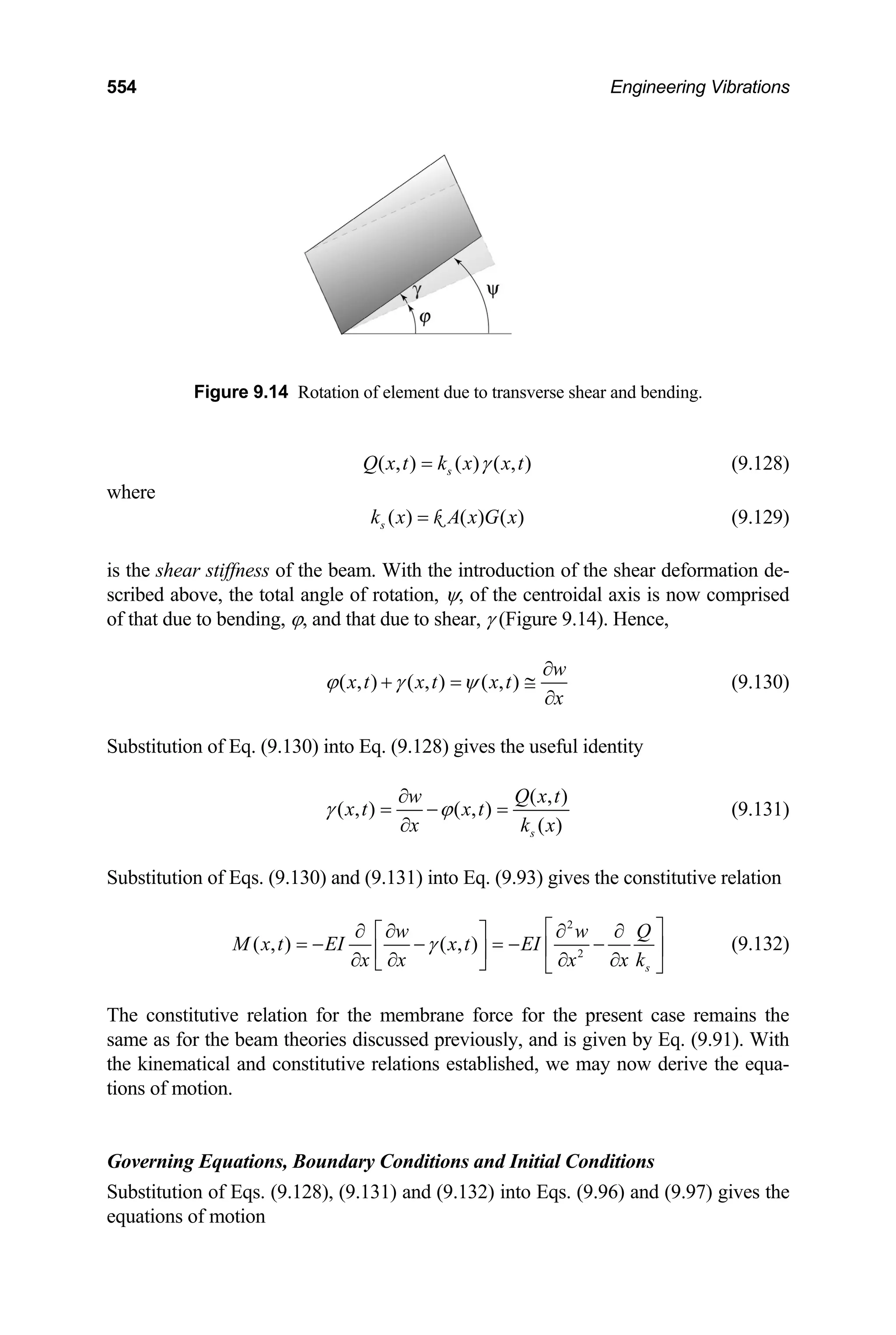
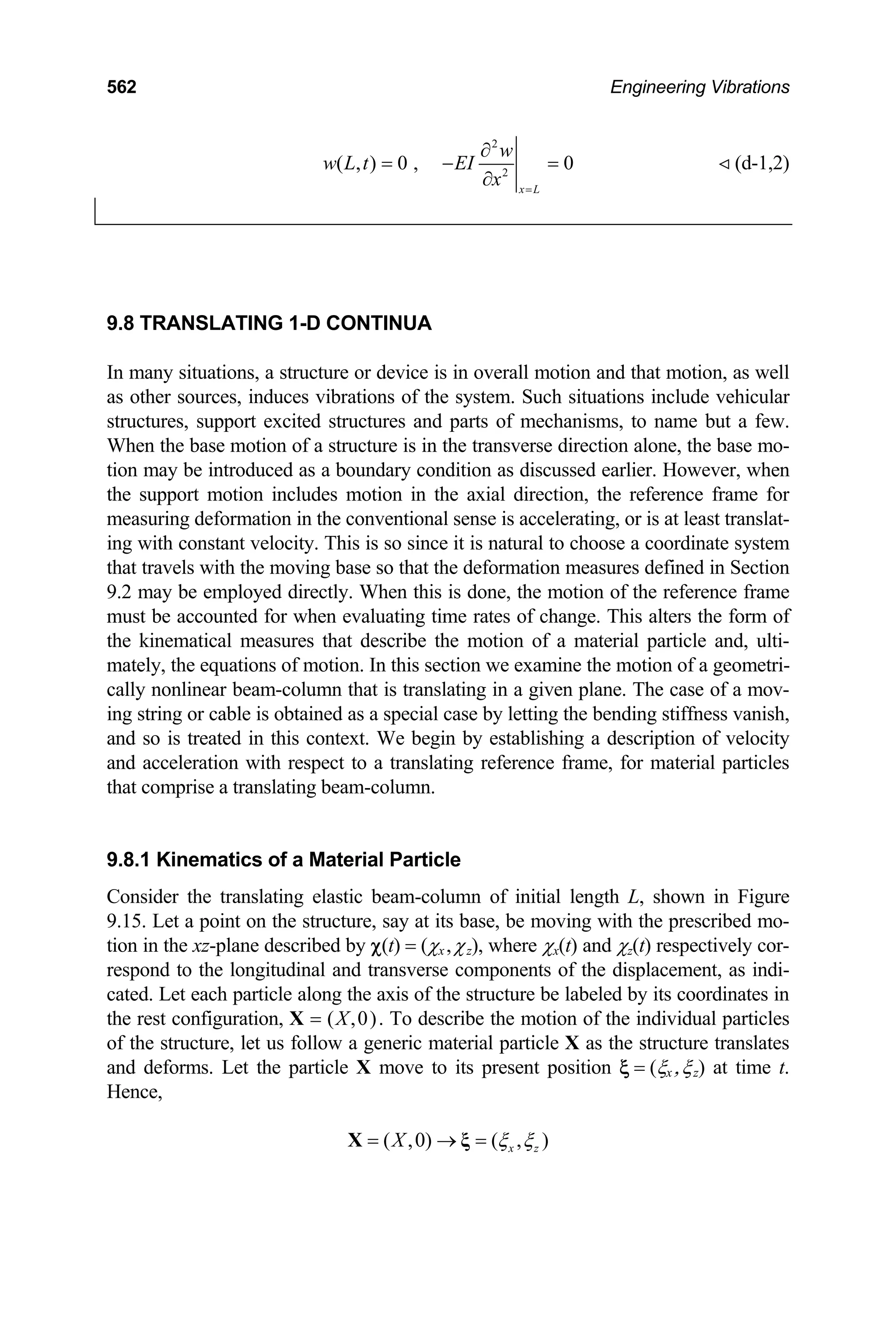
![9│ Dynamics of One-Dimensional Continua 563
Figure 9.15 Deformation of translating beam-column.
To measure the deformation, let us introduce the (fictitious) intermediate configura-
tion corresponding to the rigid body translation of the entire undeformed structure.
[Since the structure is elastic, its deformation is independent of the deformation his-
tory and thus independent of the path traversed by a material particle as it moves from
the point (X,0) to the point (ξx ,ξz ). Deformations can then be measured relative to
this convenient configuration.] Let the point x = (x,z) correspond to the location of
the image of particle X in the intermediate configuration at time t. The coordinates x
thus correspond to the projection of ξ onto the rigidly displaced image of the rod at
time t. Hence,
= +
x X χ (9.169)
or, in component form,
( )
( )
x
z
x X t
z t
χ
χ
= +
=
(9.170)
The relative deflection, the displacement of particle X at time t measured relative to
the intermediate configuration, is then
( , )
u w
= = −
u ξ x (9.171)
The velocity of particle X is then
t t t
∂ ∂ ∂
≡ = +
∂ ∂ ∂
X X
ξ x u
v
X
(9.172)
Now, from Eq. (9.169),](https://image.slidesharecdn.com/engineeringvibrations-240713005818-b85f16c0/75/Engineering-Vibrations-Engineering-Vibrations-585-2048.jpg)
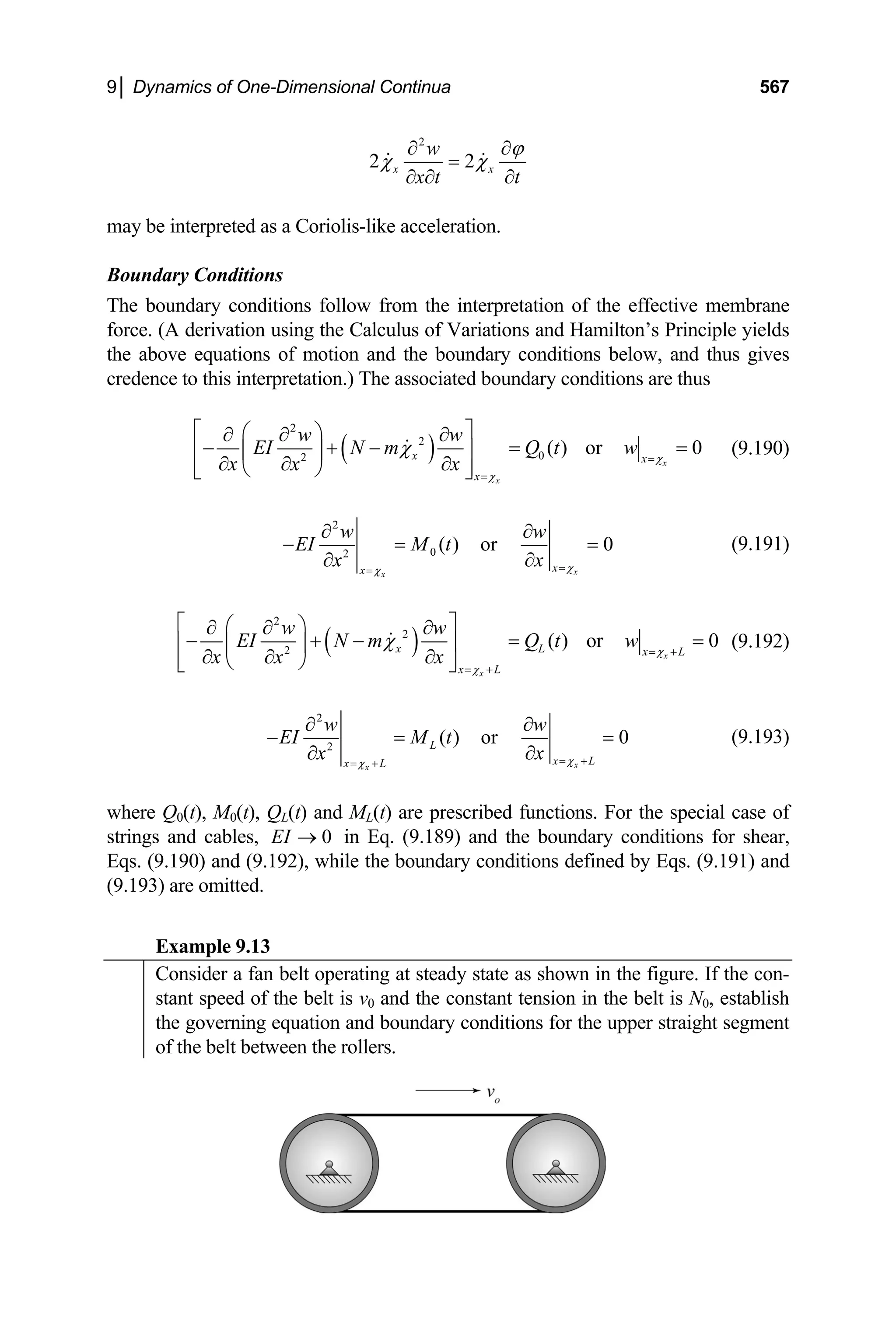
![568 Engineering Vibrations
Solution
For the present problem, EI = 0, 0
z
χ ≡ and 0 .
x v
χ = Substituting these values
into Eq. (9.189) gives the equation of motion of the belt as
( )
2 2 2
2
0 0 0
2 2
2 0
w w w
m v N mv
x t
t x
⎛ ⎞
∂ ∂ ∂
+ − − =
⎜ ⎟
∂ ∂
∂ ∂
⎝ ⎠
(a)
The boundary conditions are simply
(0, ) 0 and ( , ) 0
w t w L t
= = (b-1,2)
Example 9.14
Determine the equation of motion and associated boundary conditions for a
uniform cantilevered beam-column supporting a large point mass if
mL
m
the support undergoes the elliptical motion described parametrically by the
equations 0 0
( ) (1 cos )
u t t
α
= ∆ − Ω and 0 0 sin ,
w t
= ∆ Ω where 0 1
L
∆ and
α 1.
Solution
For the problem at hand, p = q = 0. The kinetic diagram and associated equa-
tion of motion for the point mass show that
[ ]
x
x
L
N g
χ
χ
+
≅ +
m (a)
Integrating the equation of longitudinal motion, Eq. (9.188), and incorporating
Eq. (a) gives the membrane force as
[ ]
[ ] [ ]( ) [
2
0
( , )
cos
x
x
x
L
x
L
]
x x x x
N x t N m g a dx
g m g L x g
g t
χ
χ
χ
χ χ χ χ
α
+
+
= + +
≅ + + + + − ≈ +
⎡ ⎤
= + Ω ∆ Ω
⎣ ⎦
∫
m m
m
(b)
or
0 0
( , ) cos
N x t N n t
= + Ω
g
(c)
where
0
N = m (d)
and
2
0 0
n α
= ∆ Ω (e)
Next,](https://image.slidesharecdn.com/engineeringvibrations-240713005818-b85f16c0/75/Engineering-Vibrations-Engineering-Vibrations-590-2048.jpg)
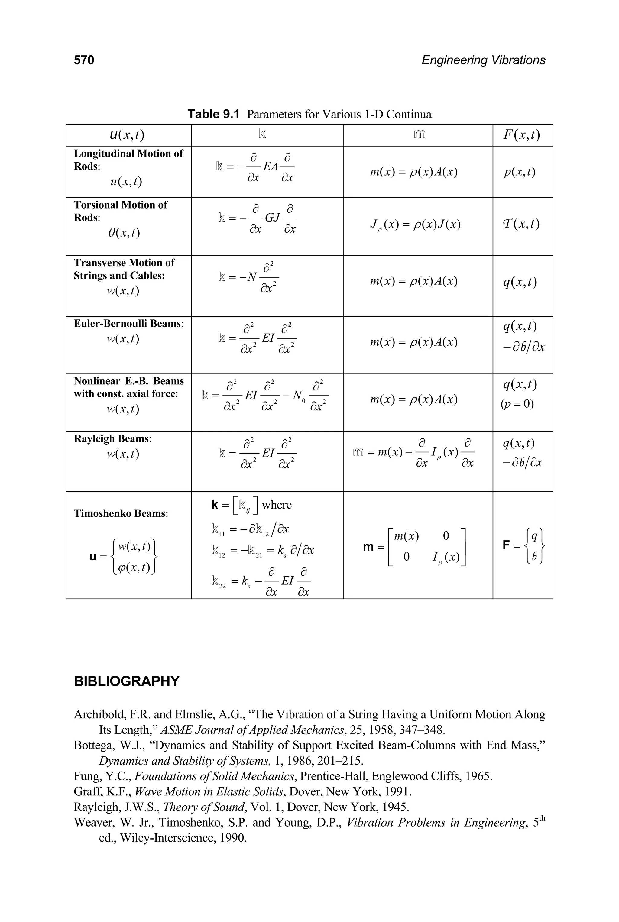
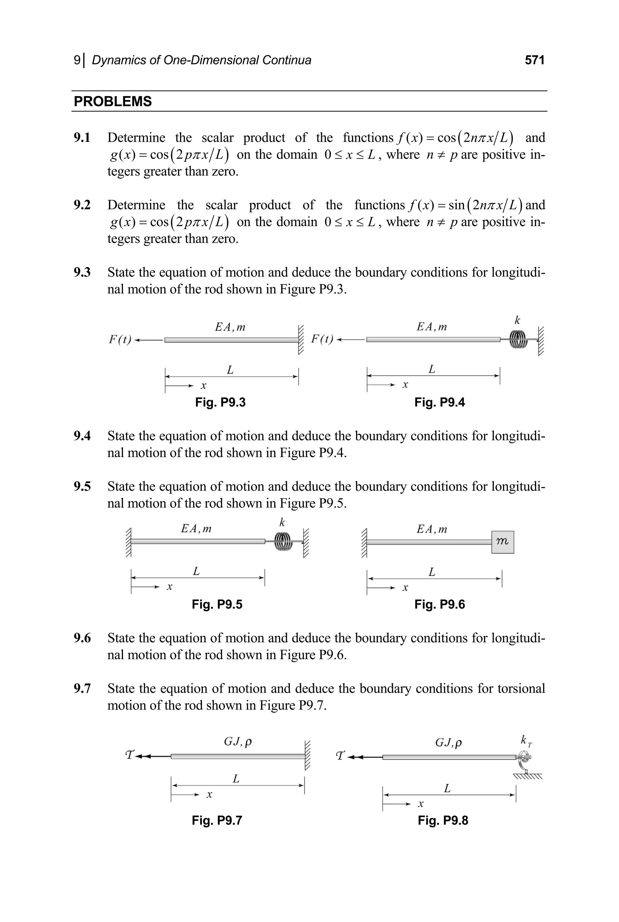
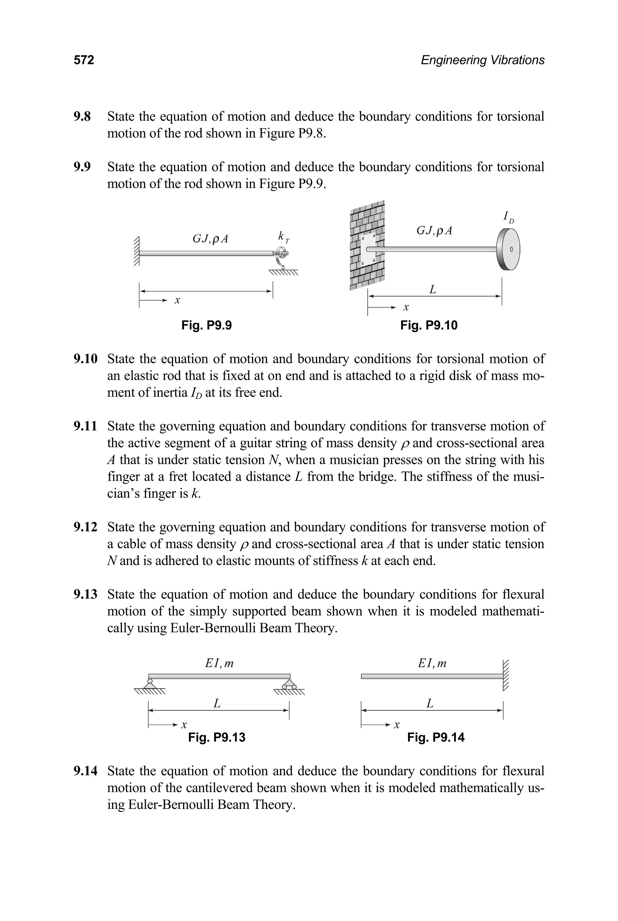
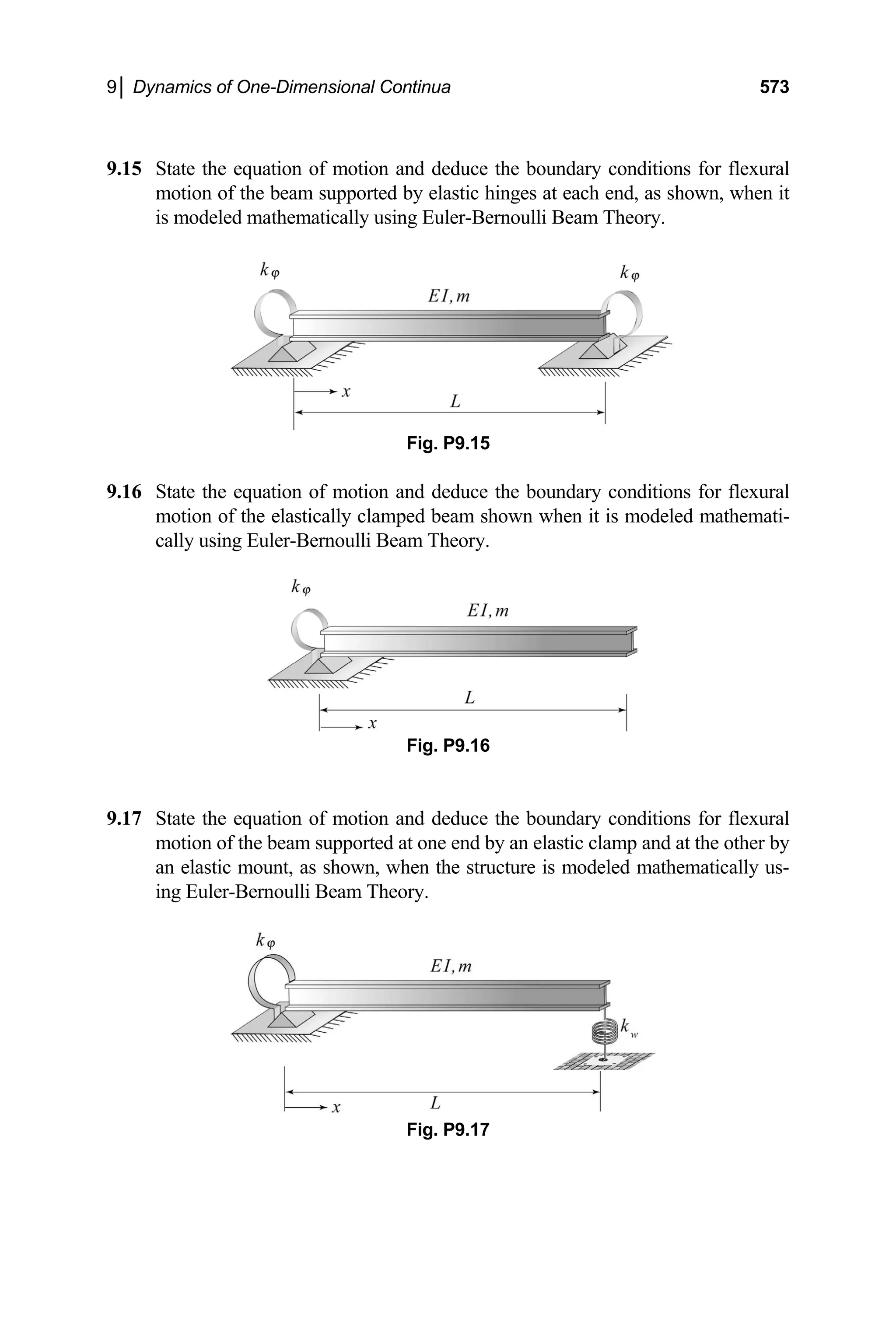
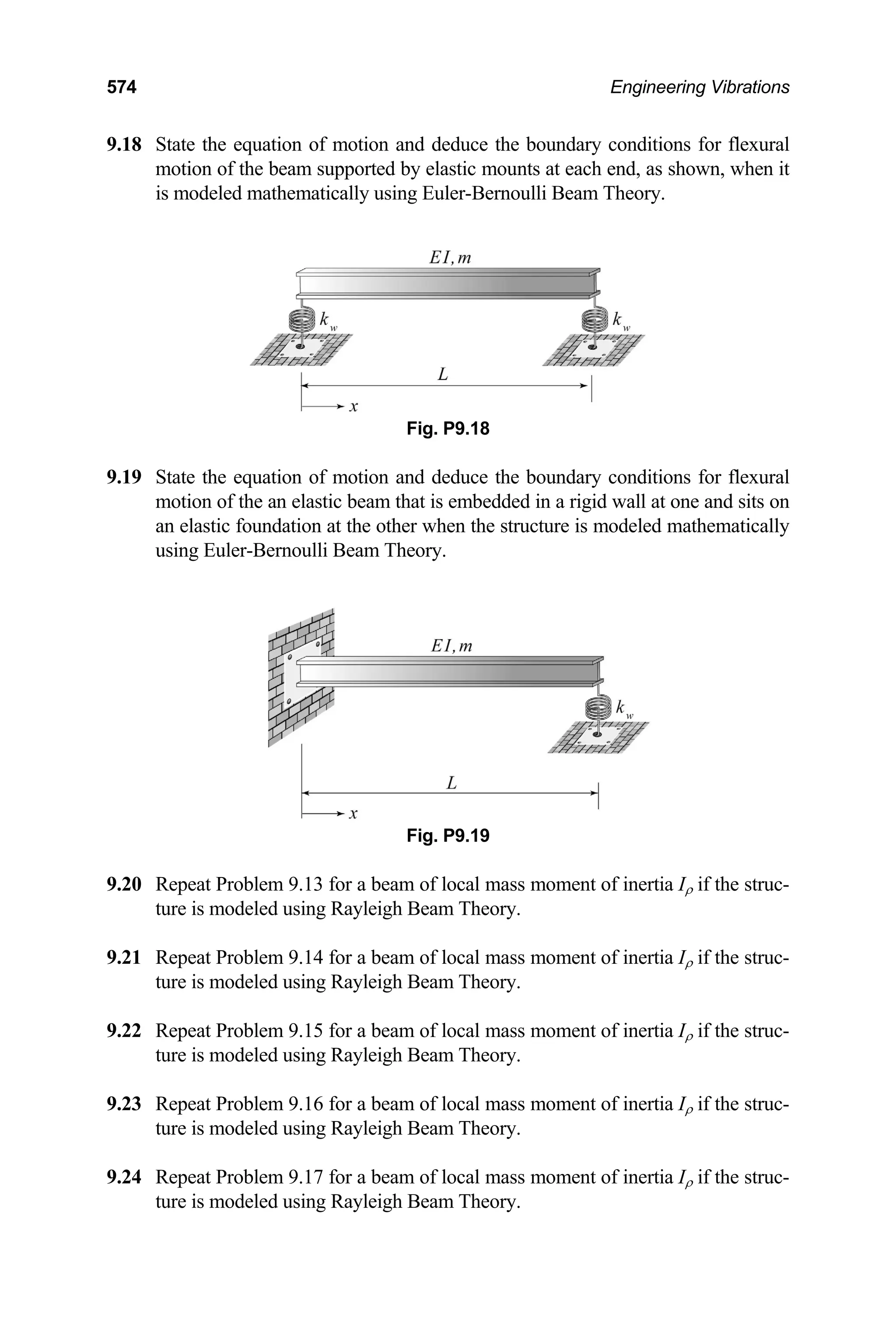
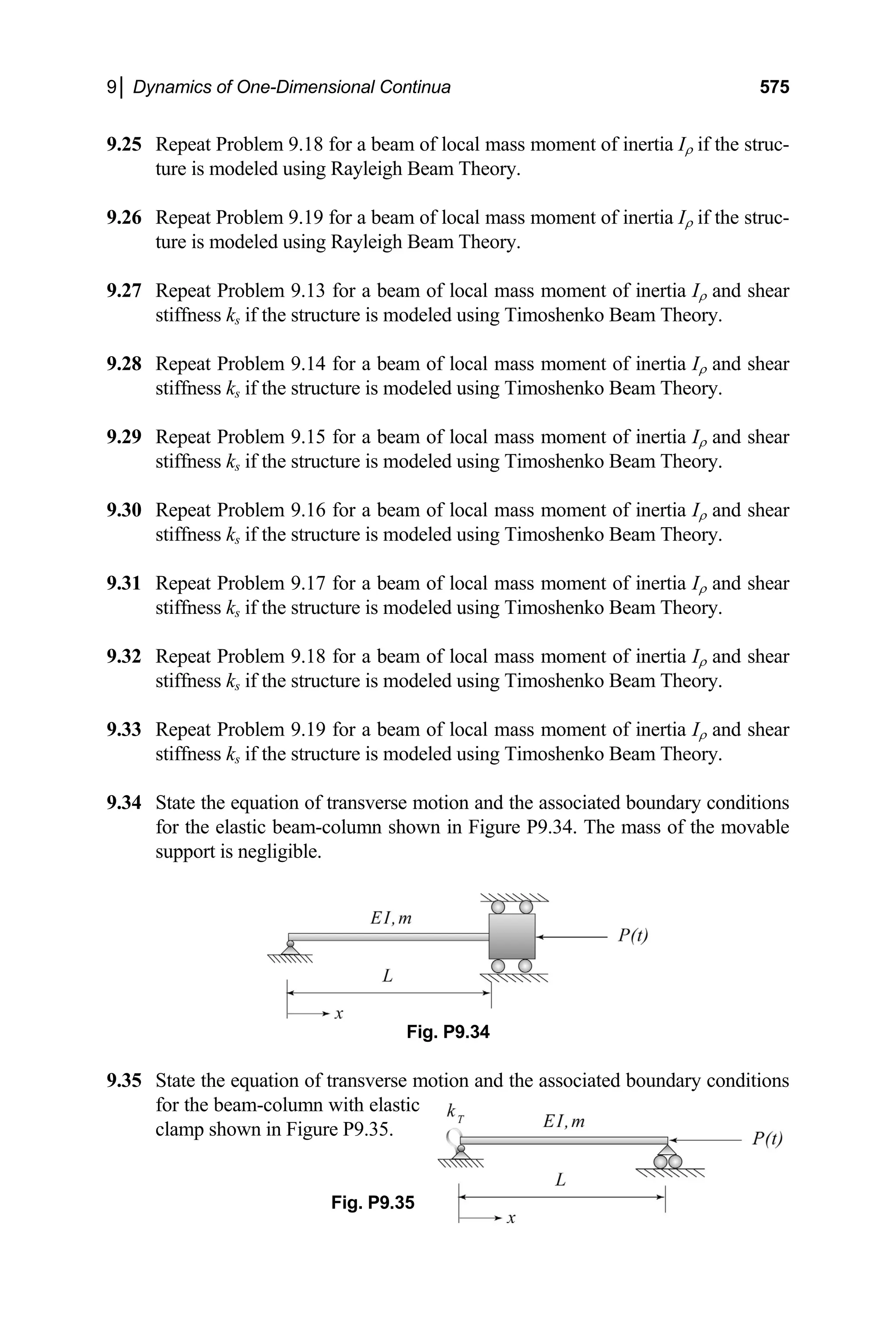
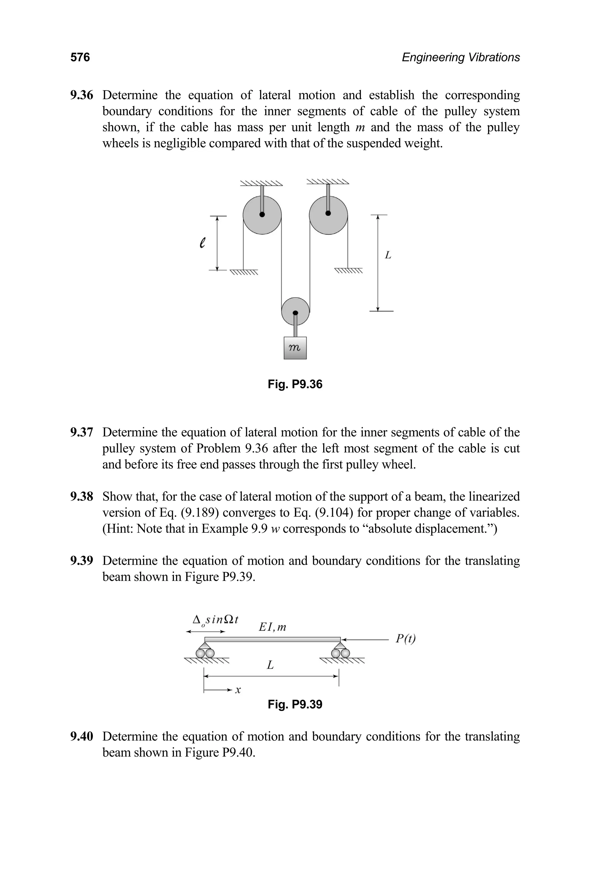
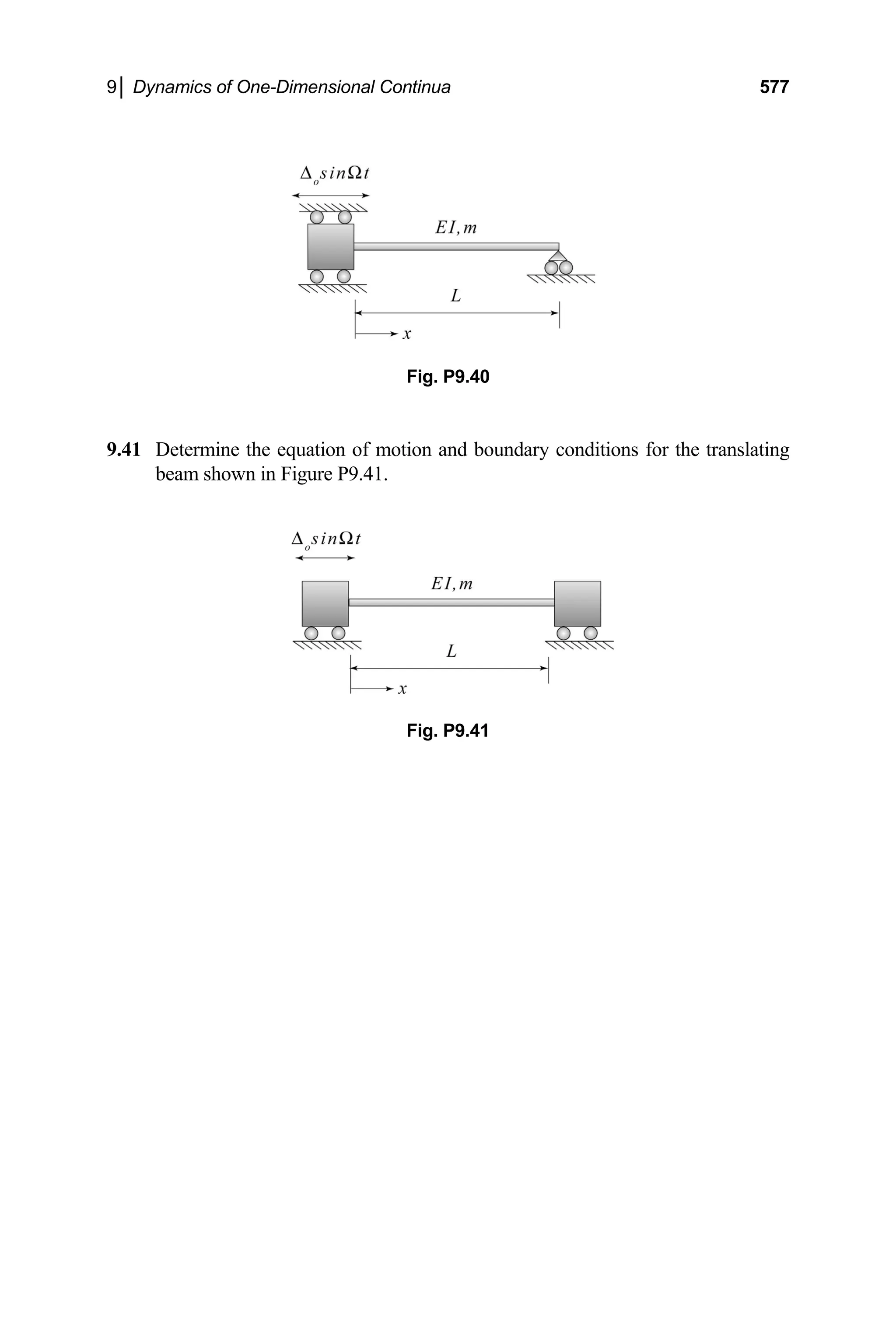

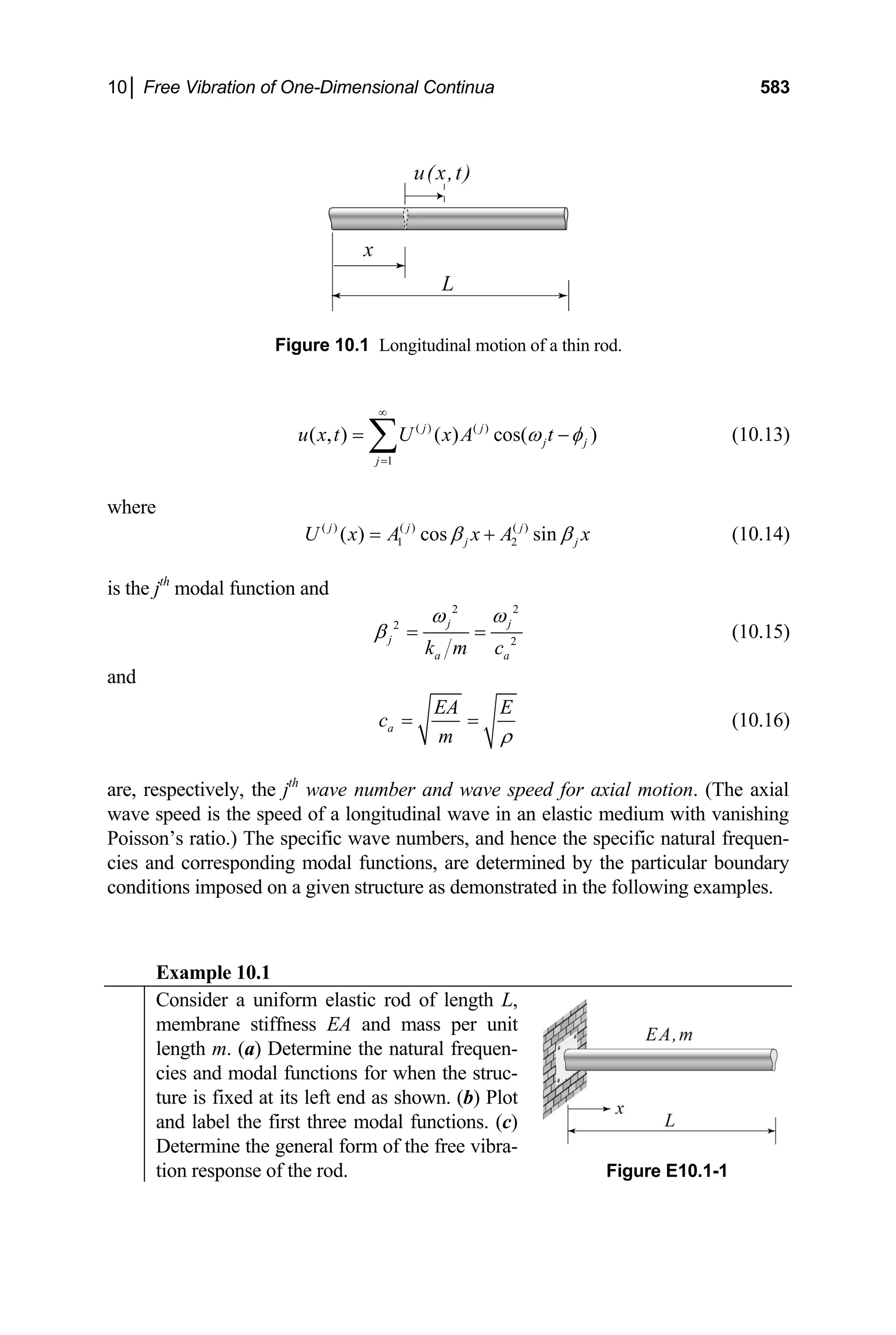
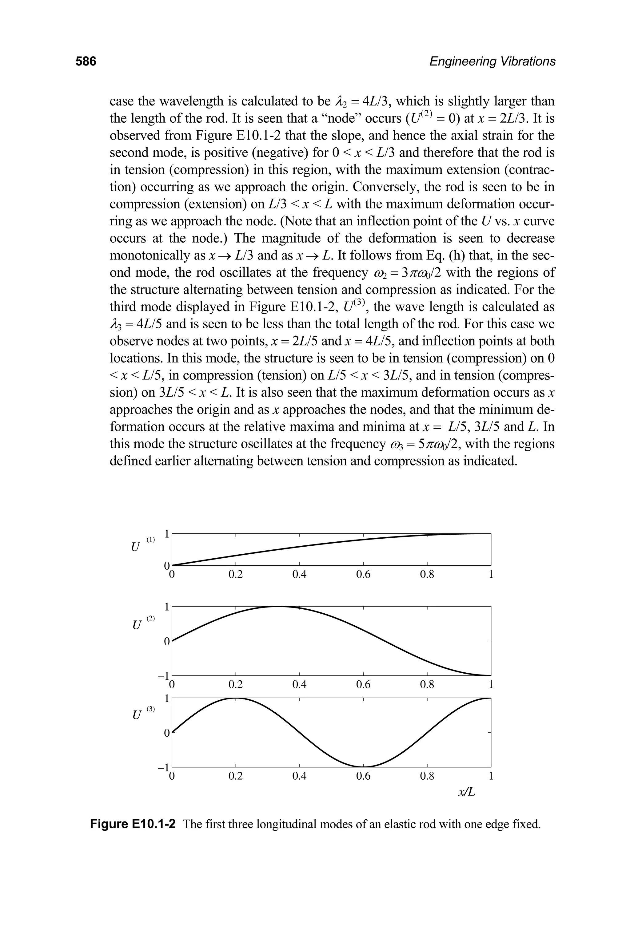
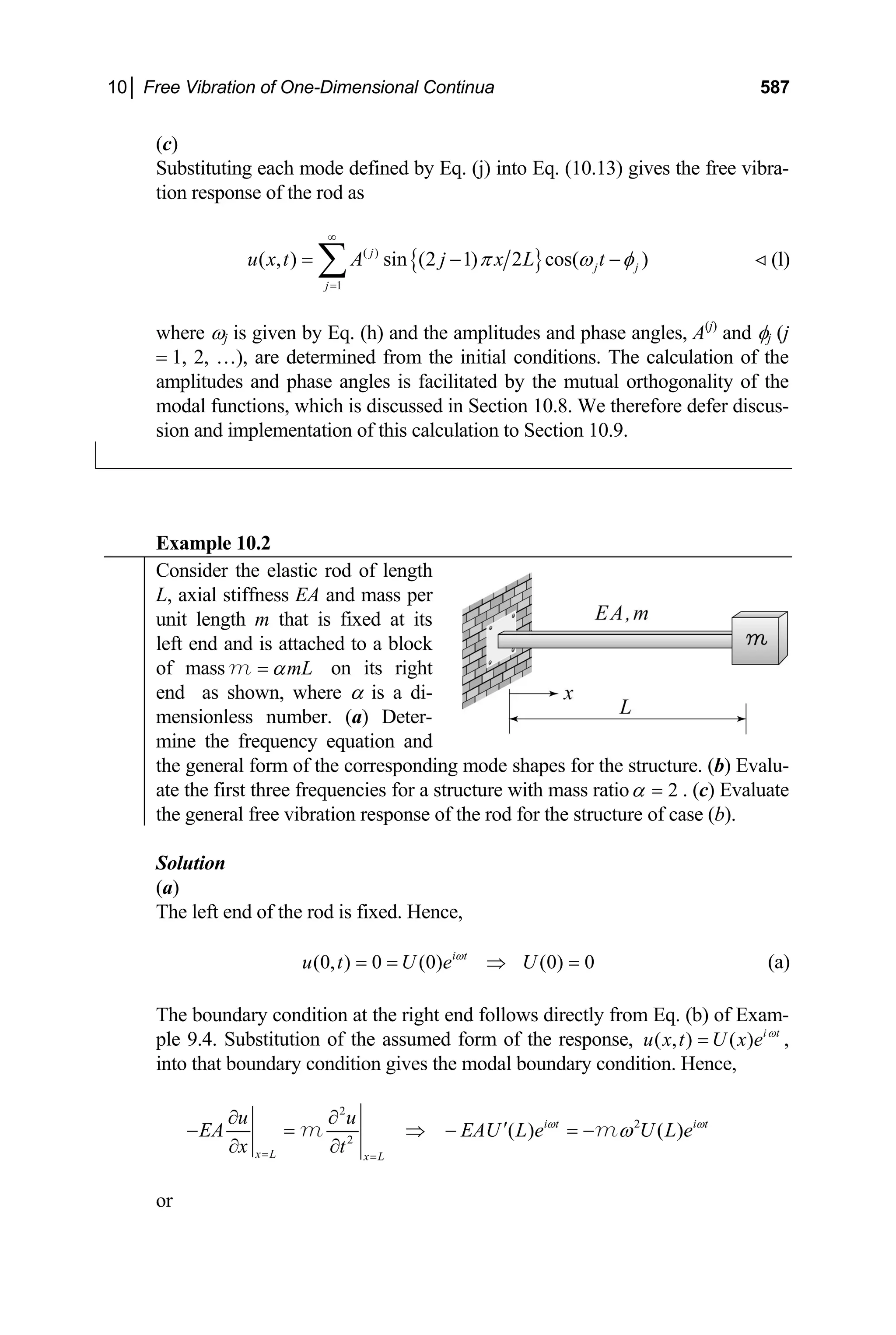
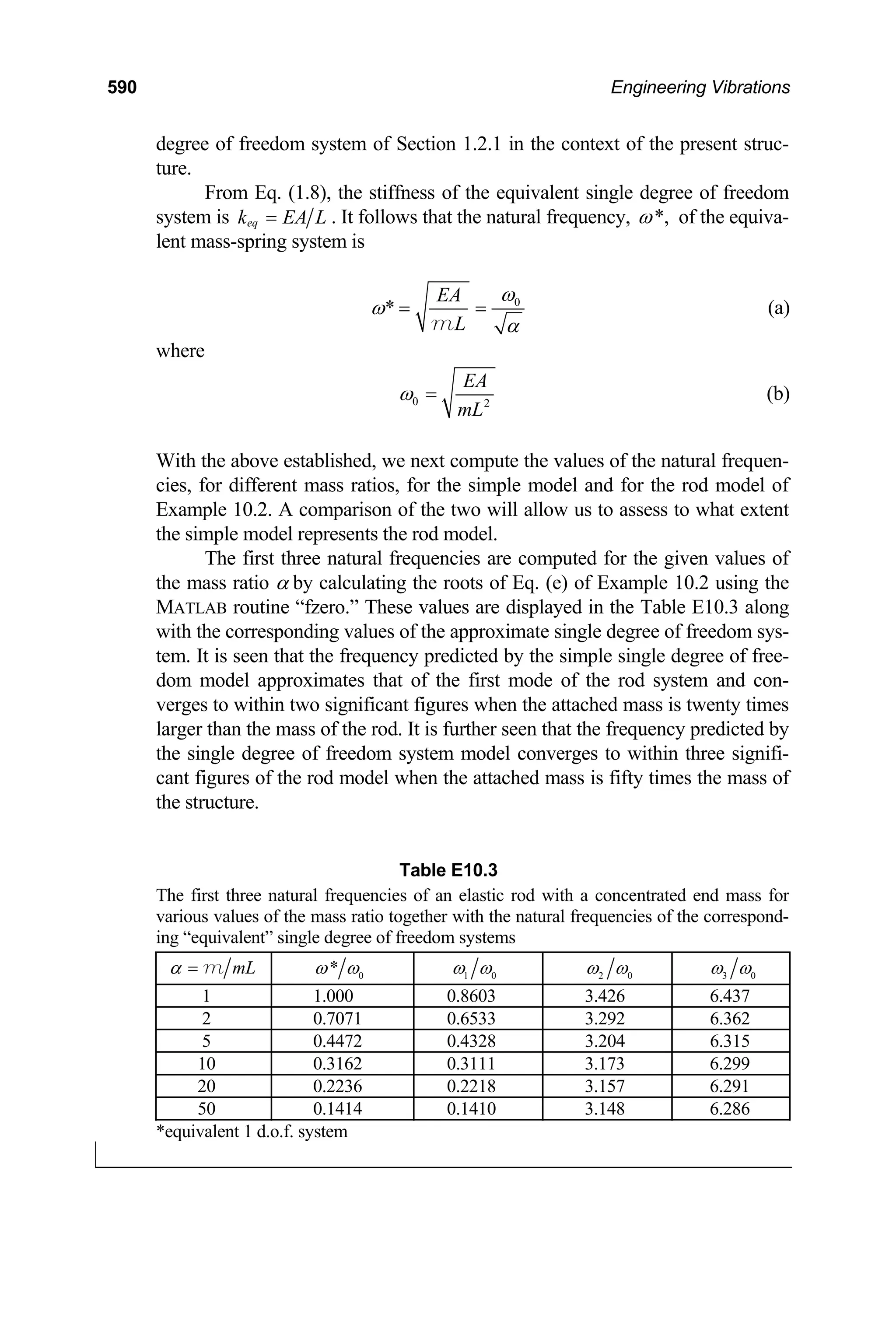
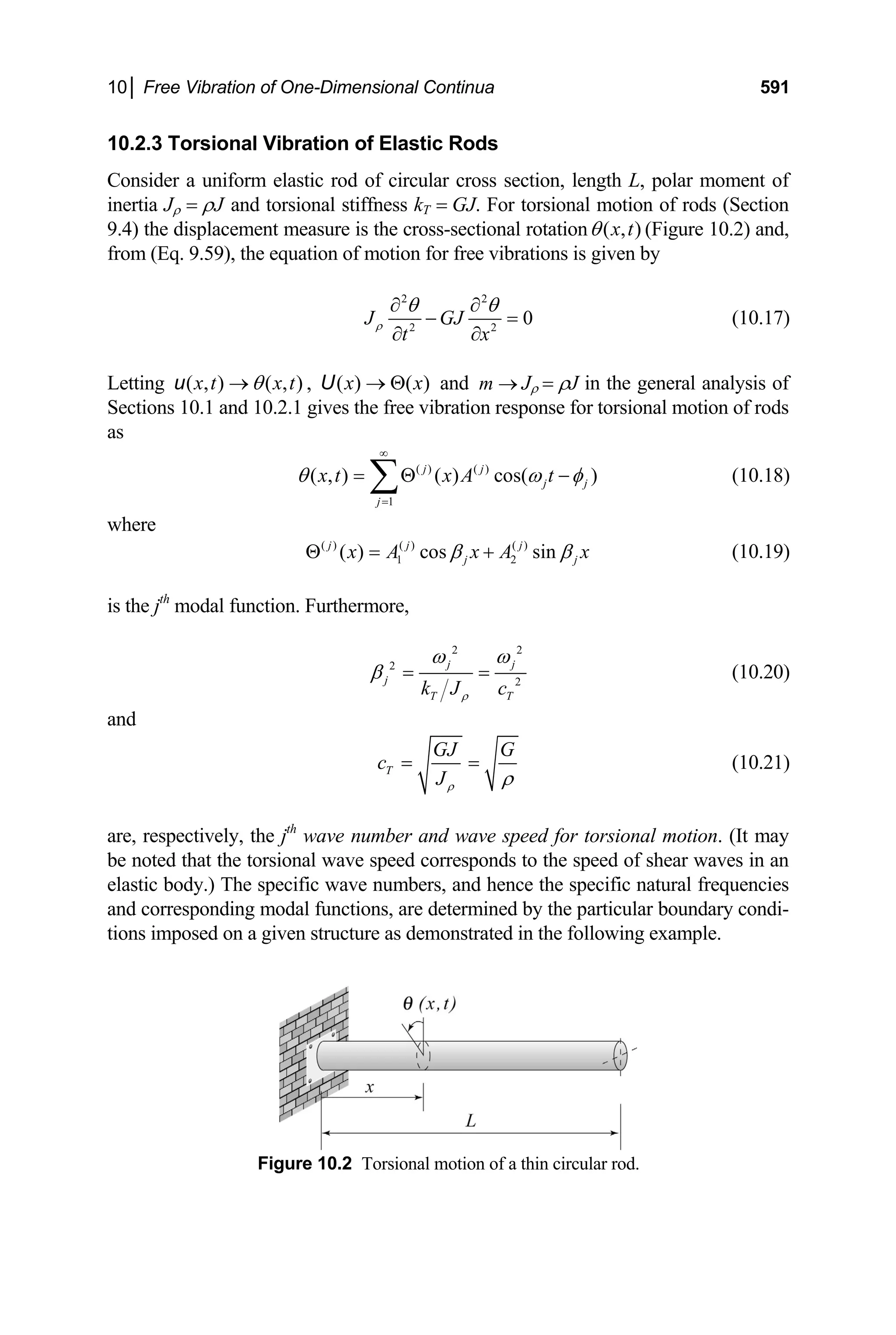
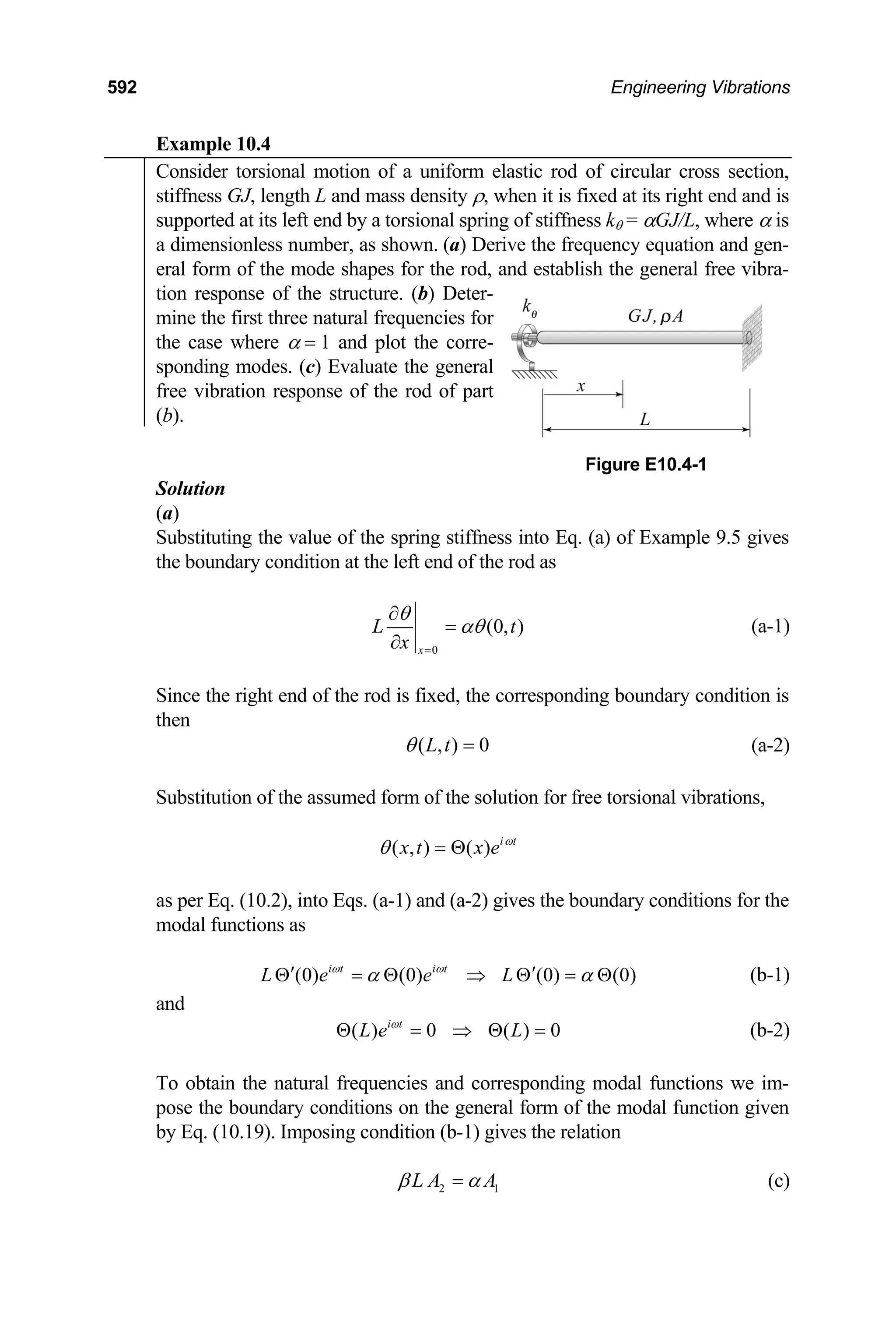
![10│ Free Vibration of One-Dimensional Continua 593
Imposing condition (b-2) on the general form of the modal function and substi-
tuting Eq. (c) into the resulting expression gives
[ ]
2
cos sin 0
A
L L L
β β α β
α
+ =
It may be seen from Eq. (10.19) and Eq. (c) that A2 = A1 = 0 yields the trivial
solution, as does β = 0. Hence, for nontrivial solutions, the expression within
the brackets must vanish. We thus obtain the frequency equation for the rod in
question,
cos sin 0
L L L
β β α β
+ = (d)
Equation (d) may be solved numerically to obtain the natural frequencies of the
rod. Substituting Eq. (c) into Eq. (10.19) gives the modal function associated
with the jth
natural frequency as
( )
2
( )
( ) cos sin
j
j
j j j
A
x L x
β β α β
α
x
⎡ ⎤
Θ = +
⎣ ⎦
Since the value of ( )
2
j
A is arbitrary we shall set ( )
2
.
j
A α
= The jth
modal function
is then
( )
( ) cos sin
j
j j j
x L x x
β β α β
Θ = + (e)
With the frequencies determined from Eq. (d), substituting Eq. (e) into Eq.
(10.18) gives the free vibration response of the rod as
( )
1
( , ) cos sin cos( )
j
j j j j
j
x t A L x x t j
θ β β α β ω φ
∞
=
⎡ ⎤
= +
⎣ ⎦
∑ − (f)
(b)
The first three roots of Eq. (d) are determined numerically using the MATLAB
routine “fzero,” which gives, for systems with 1
α = ,
1 2 3
2.029 , 4.913 , 7.979, ...
L L L
β β β
= = = (g)
The associated natural frequencies are obtained by substituting the above roots
into Eq. (10.20). Hence,
1 0 2 0 3 0
2.029 , 4.913 , 7.979 , ...
ω ω ω ω ω ω
= = = (h)](https://image.slidesharecdn.com/engineeringvibrations-240713005818-b85f16c0/75/Engineering-Vibrations-Engineering-Vibrations-615-2048.jpg)
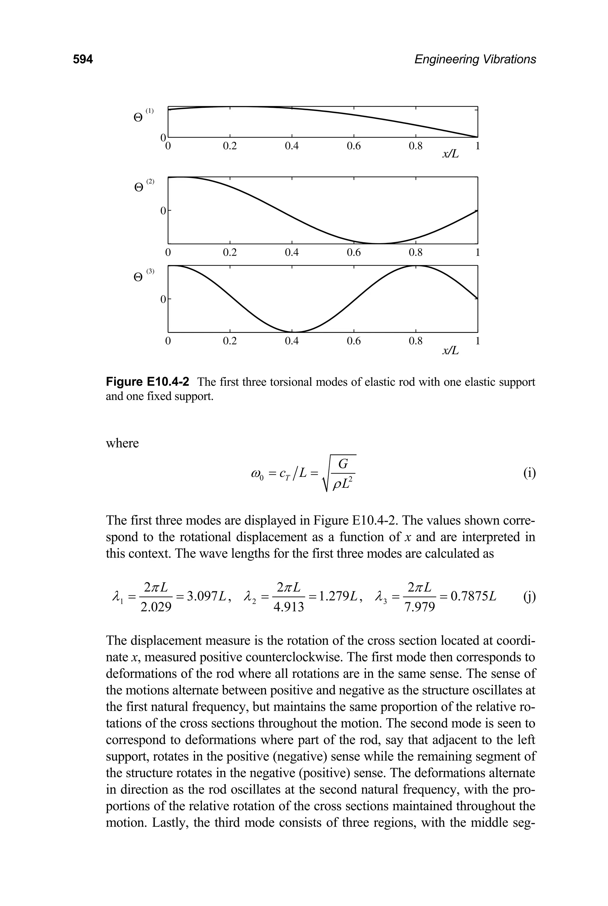
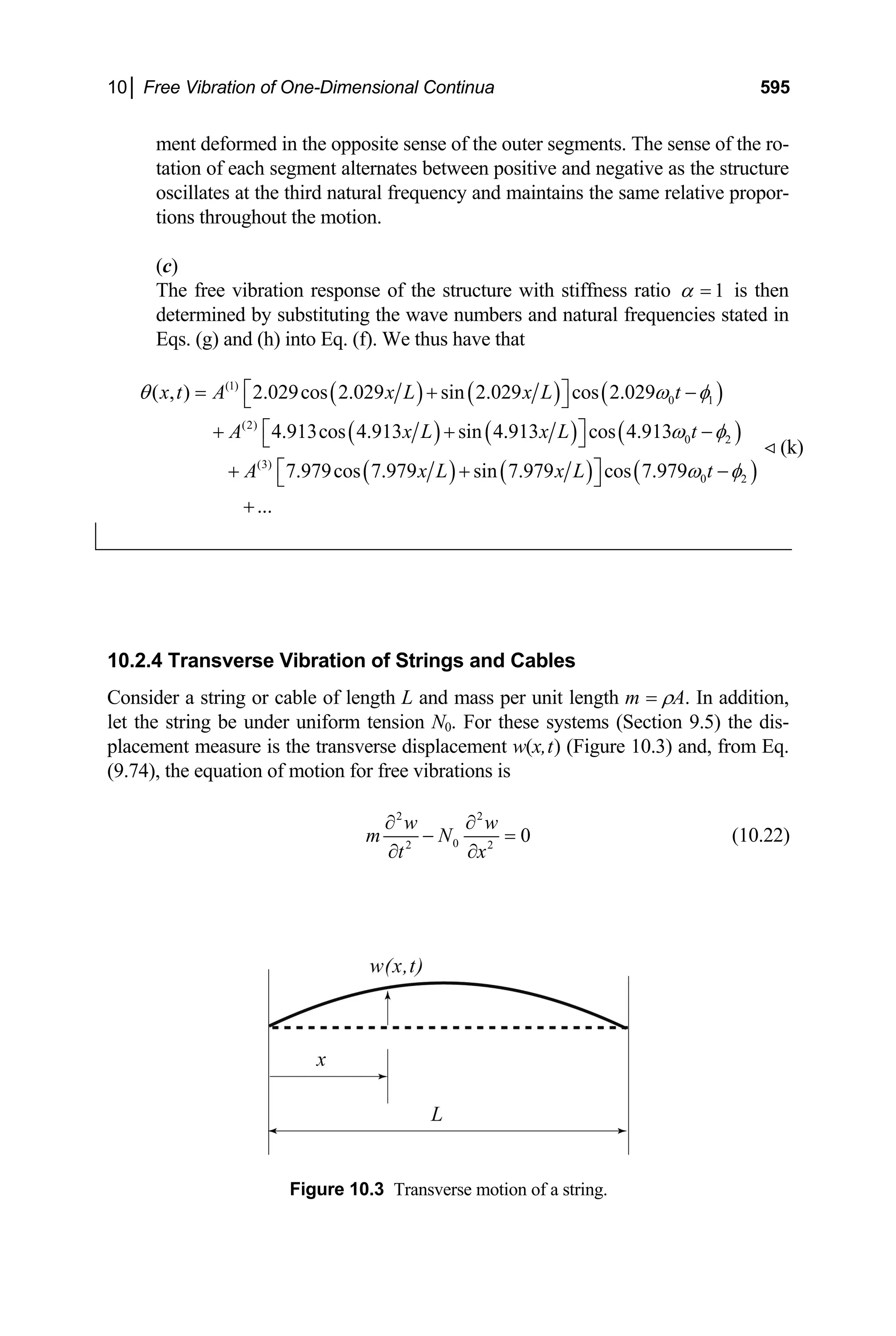
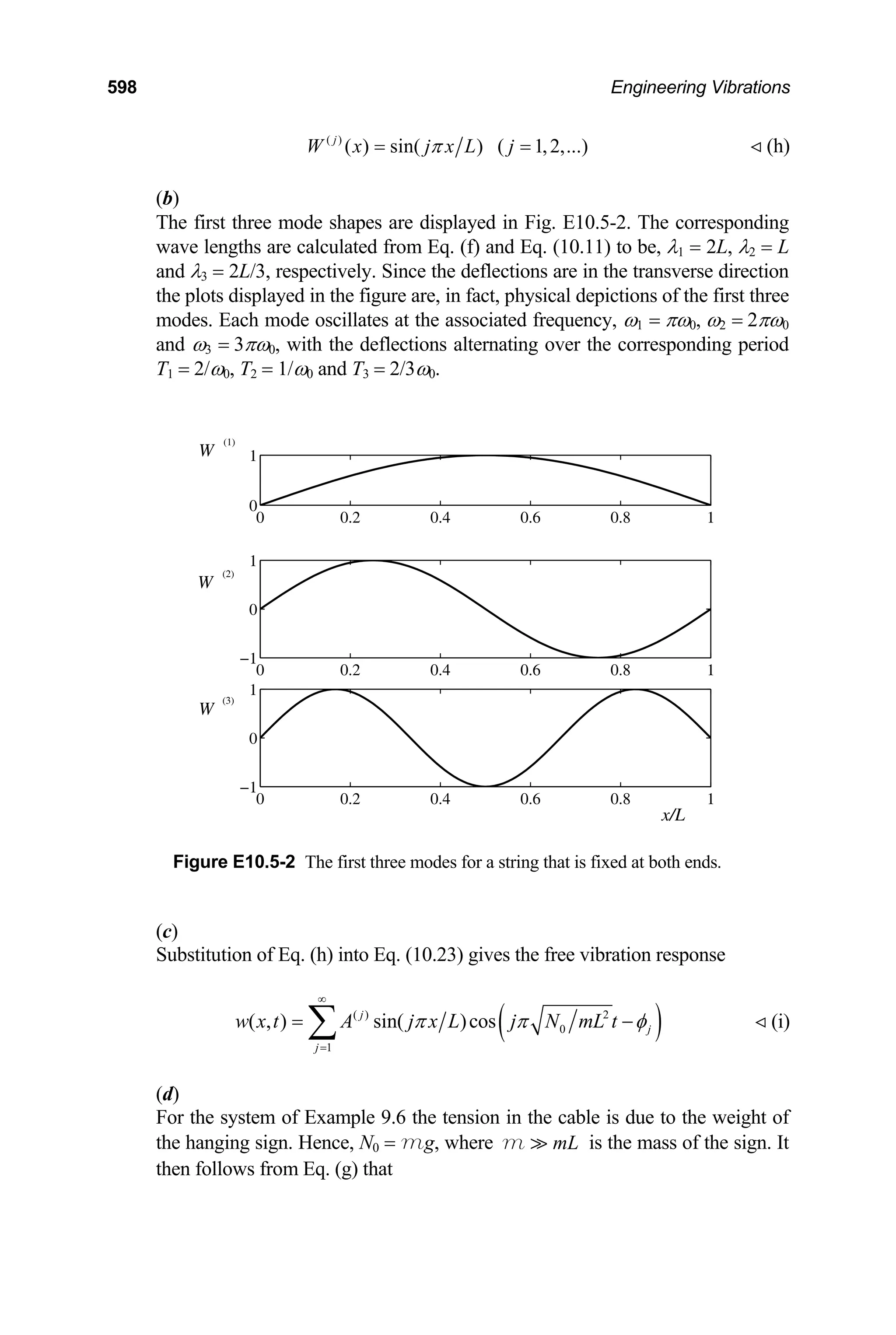
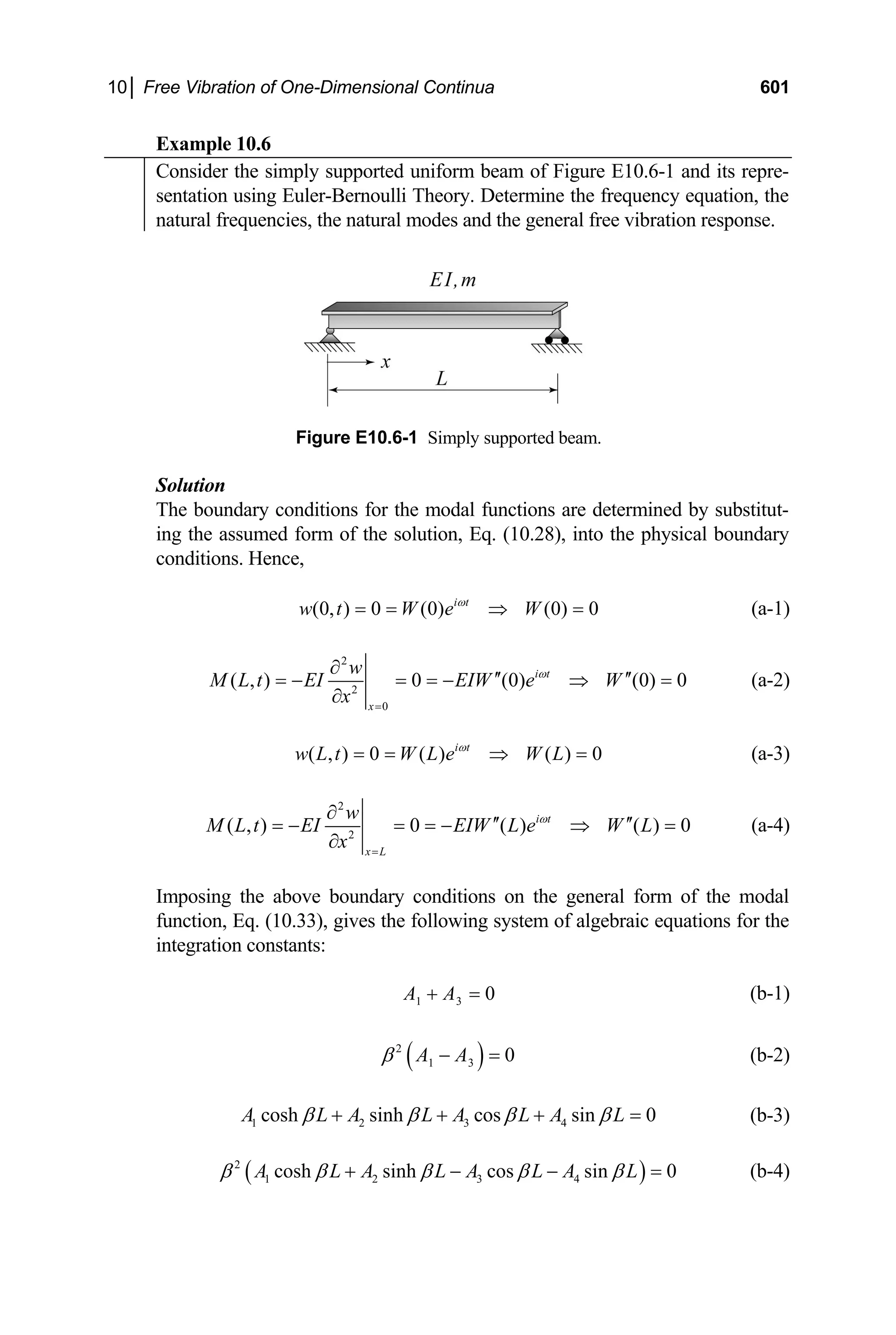
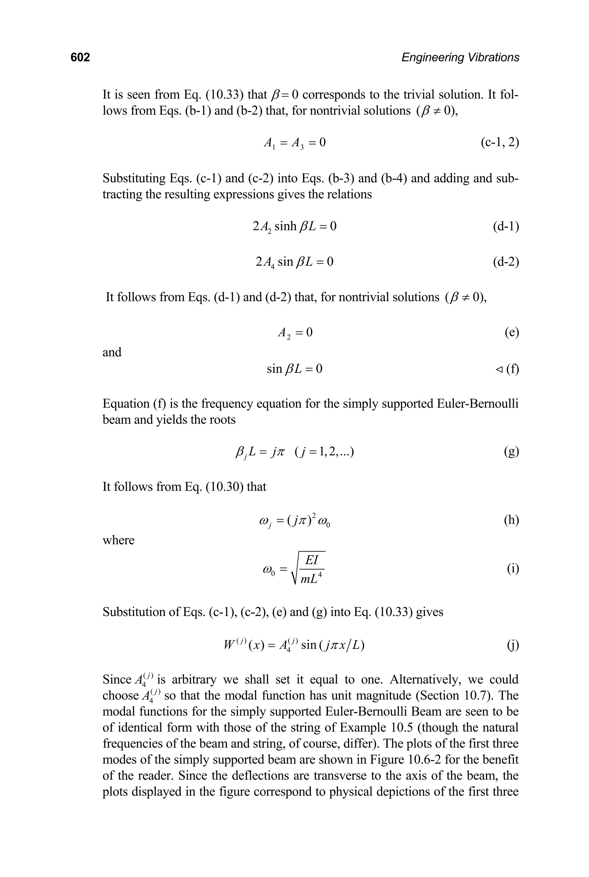
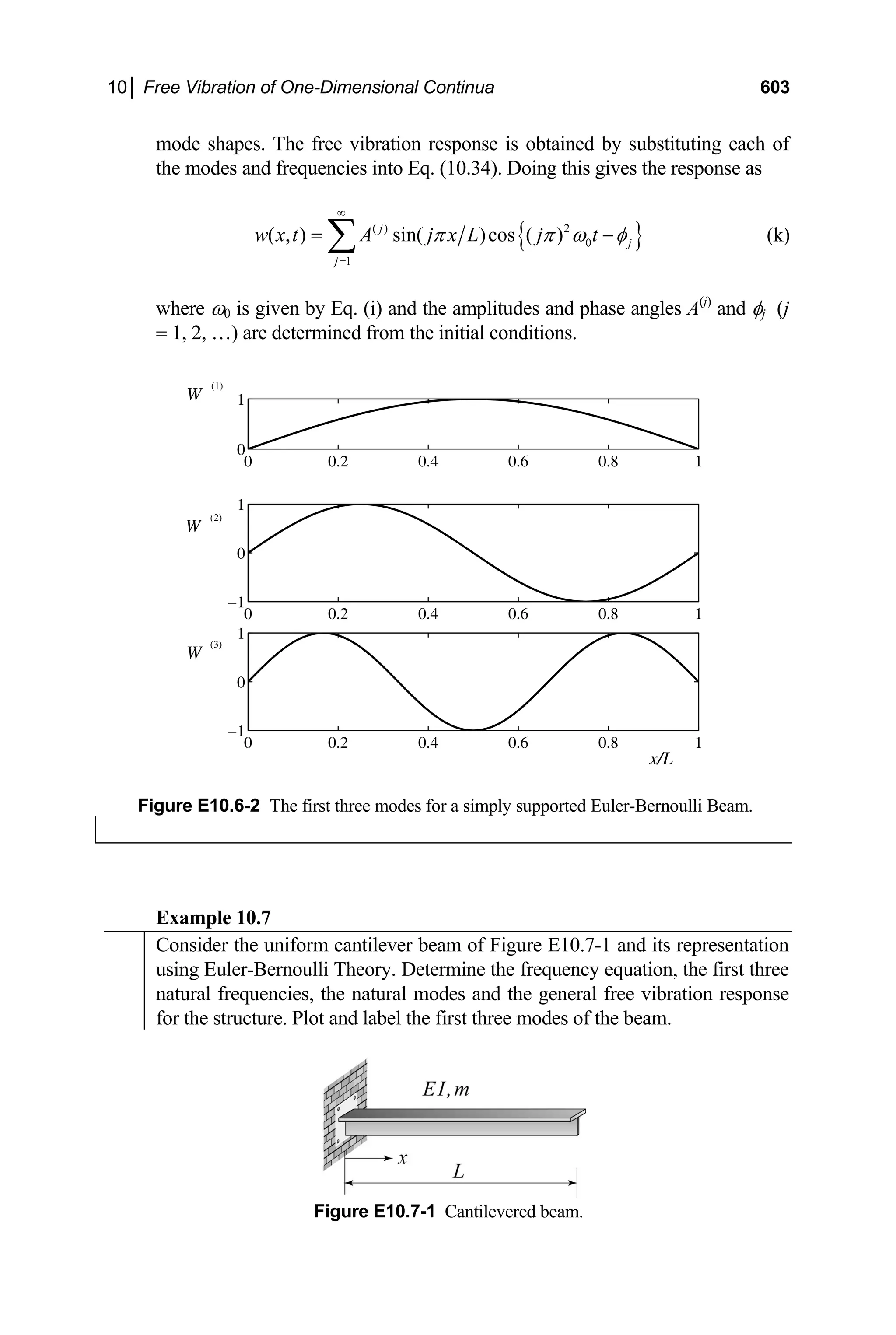
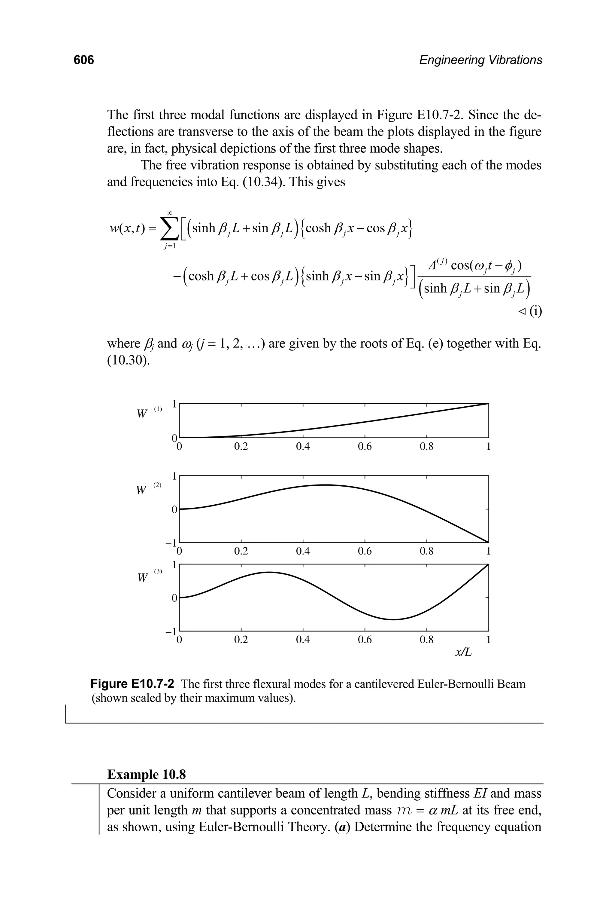
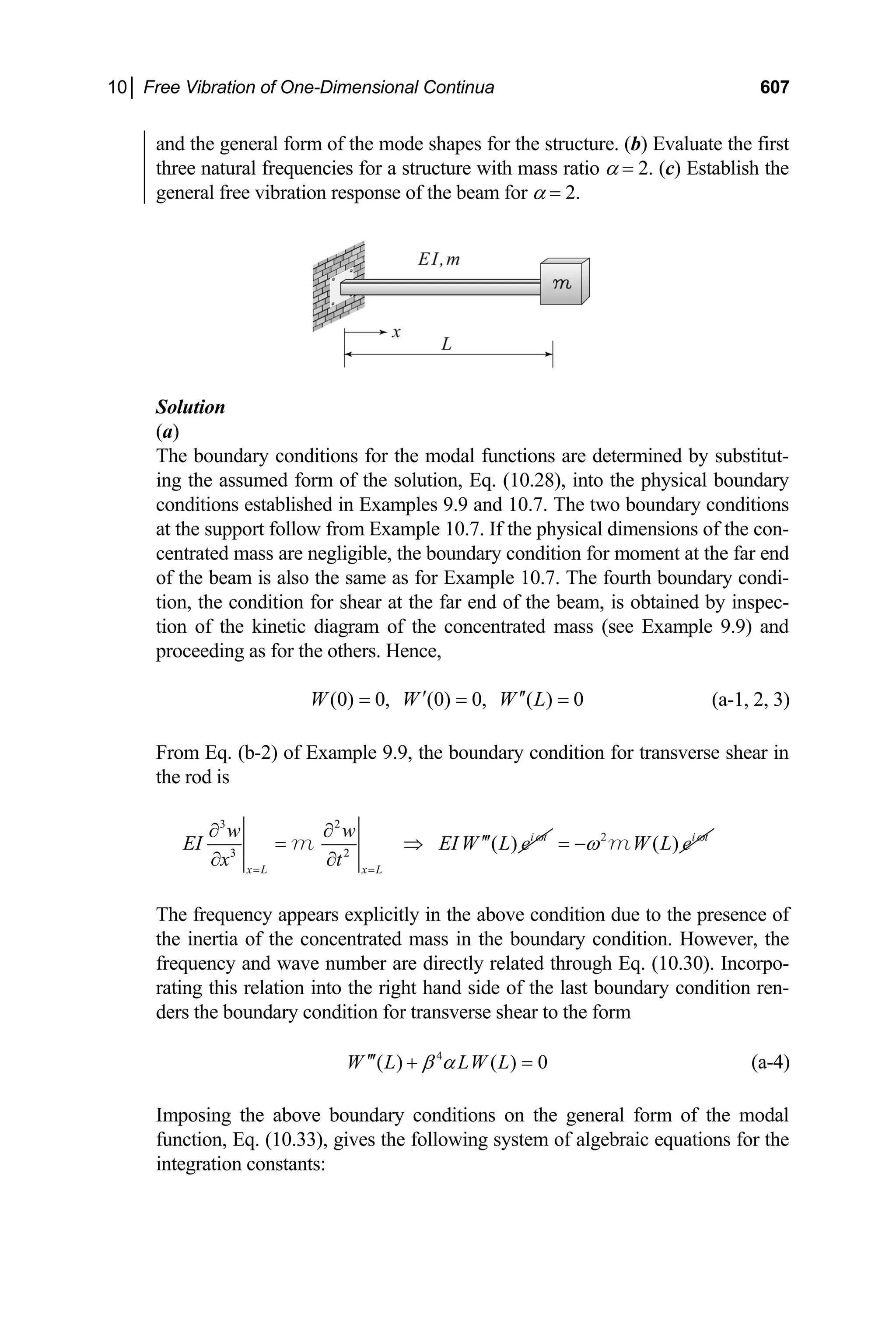
![608 Engineering Vibrations
1 3 0
A A
+ = (b-1)
( )
2 4 0
A A
β + = (b-2)
( )
2
1 2 3 4
cosh sinh cos sin 0
A L A L A L A L
β β β β β
+ − − = (b-3)
( )
( )
3
1 2 3 4
3
1 2 3 4
sinh cosh sin cos
cosh sinh cos sin 0
A L A L A L A L
L A L A L A L A L
β β β β β
β αβ β β β β
+ + −
− + + + =
(b-4)
As for the previous example, it is seen from Eqs. (b-1) and (10.33) that β = 0
corresponds to the trivial solution. We can therefore divide Eqs. (b-2), (b-3)
and (b-4) by β, β 2
and β 3
, respectively. Eliminating A3 and A4 in the above
system by substituting Eqs. (b-1) and (b-2) into Eqs. (b-3) and (b-4) results in
the pair of algebraic equations
1 2
(cosh cos ) (sinh sin ) 0
A L L A L L
β β β β
+ + + = (c-1)
[ ]
[ ]
1
2
(sinh sin ) (cosh cos )
(cosh cos ) (sinh sin ) 0
A L L L L L
A L L L L L
β β αβ β β
β β β β β
− + −
+ + + − =
(c-2)
Arranging Eqs. (c-1) and (c-2) in matrix form and, since we are interested in
nontrivial solutions, setting the determinant of the coefficients of the integra-
tion constants to zero results in the frequency equation
( ) ( )
1 cosh cos sinh cos cosh sin 0
L L L L L L L
β β αβ β β β β
+ + − = (d)
The roots of the above equation yield the wave numbers, and hence the natural
frequencies, for the given structure.
Equation (c-1) gives A2 in terms of A1. Substituting this expression into
Eqs. (b-1) and (b-2) gives the remaining constants, A3 and A4, in terms of A1.
Substituting the resulting expressions into Eq. (10.33) then gives modal func-
tions for the structure. We thus obtain,
{ }
{ }
( ) ( )
1
( ) (sinh sin ) cosh cos
(cosh cos ) sinh sin
j j
j j j j
j j j j
W x A L L x x
L L x
β β β β
β β β β
⎡
= + −
⎣
⎤
− + −
⎦
x
( 1,2,...
j = )
where
( ) ( )
1 1 (sinh sin )
j j
j j
A A L
β β
= + L](https://image.slidesharecdn.com/engineeringvibrations-240713005818-b85f16c0/75/Engineering-Vibrations-Engineering-Vibrations-630-2048.jpg)
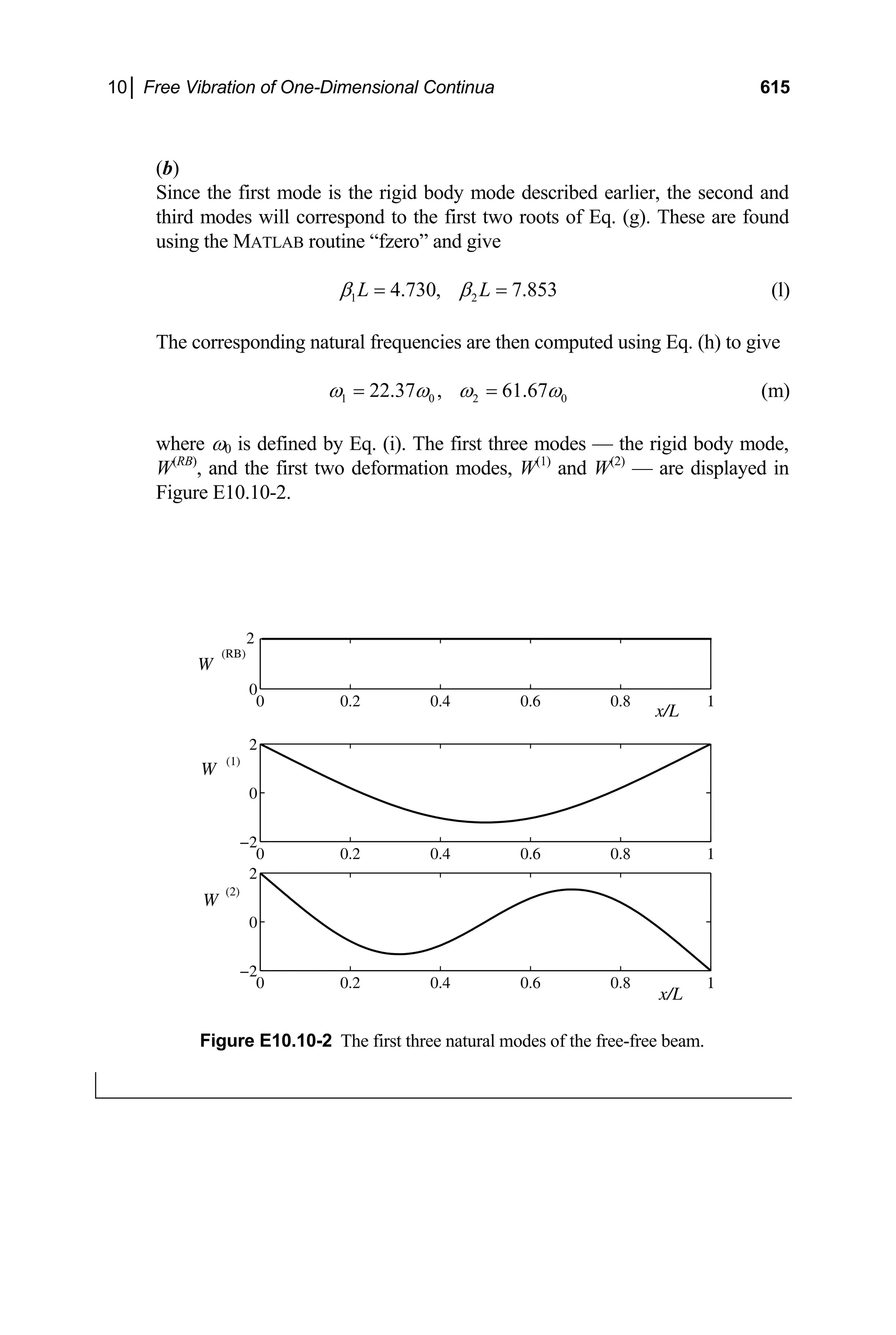
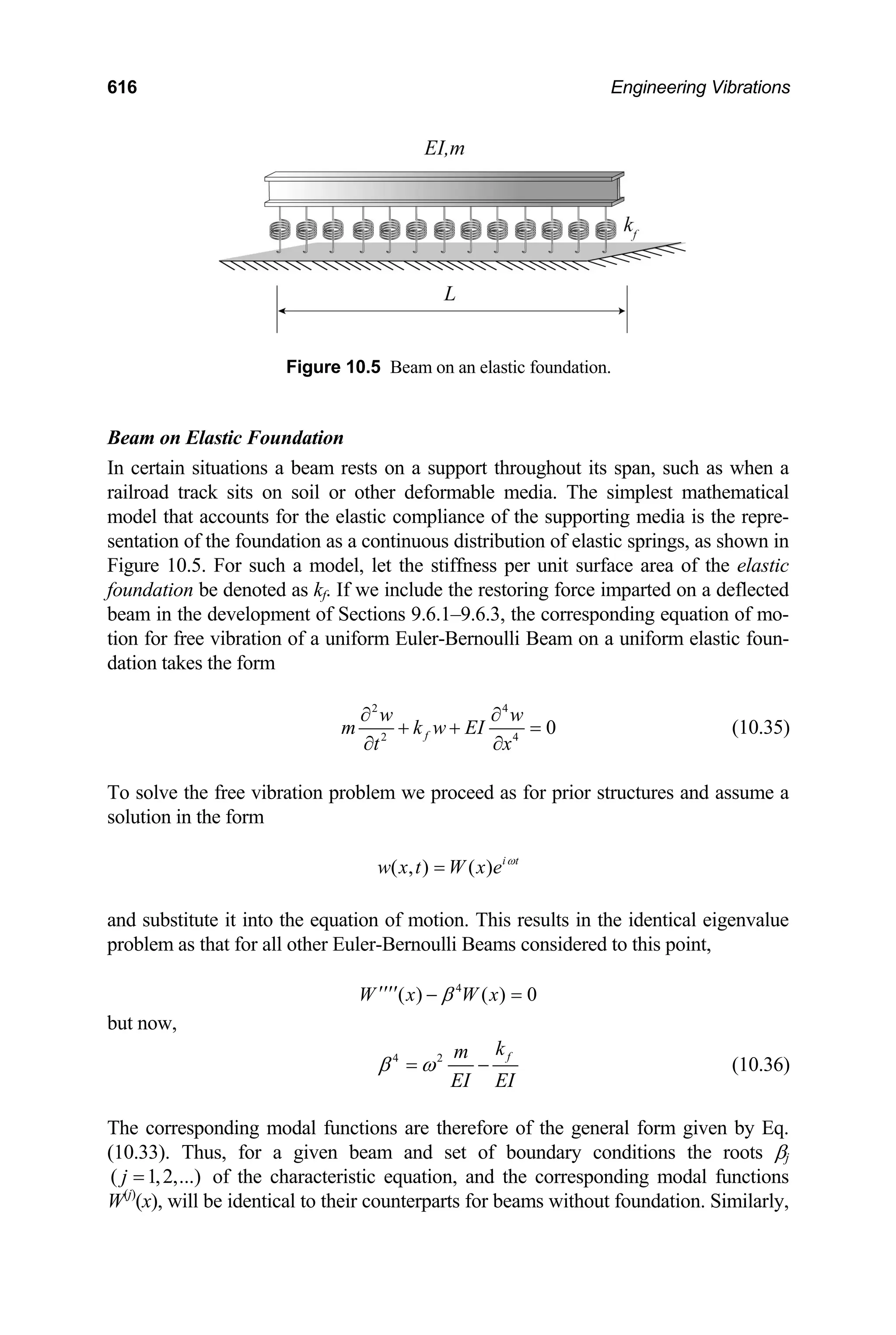
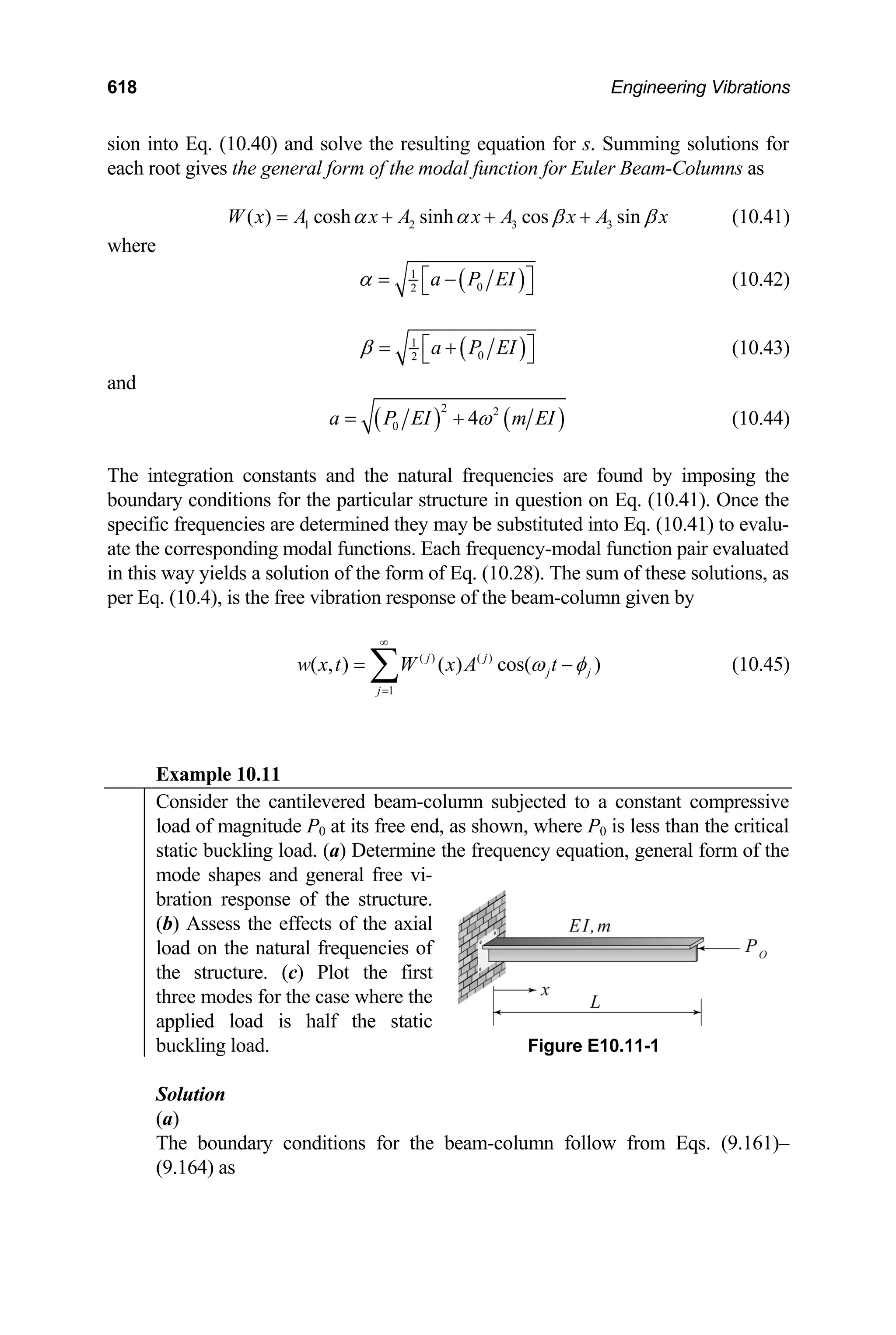
![10│ Free Vibration of One-Dimensional Continua 619
0
(0, ) 0, 0
x
w
w t
x =
∂
= =
∂
(a-1, 2)
2 3
0
2 3
0, 0
x L x L
w w w
EI EI P
x
x x
= =
⎡ ⎤
∂ ∂ ∂
− = − +
⎢ ⎥
∂
∂ ∂
⎣ ⎦
= (a-3, 4)
Substituting Eq. (10.28) into the above conditions gives the corresponding
boundary conditions for the modal functions as
(0) 0, (0) 0
W W′
= = (c-1, 2)
0
( ) 0, ( ) ( ) 0
W L EIW L PW L
′′ ′′′ ′
= + = (c-3, 4)
We next impose the modal boundary conditions, Eqs. (c-1)–(c-4), on Eq.
(10.41). This gives the following system of algebraic equations for the integra-
tion constants:
1 3 0
A A
+ = (d-1)
2 4 0
A A
α β
+ = (d-2)
(d-3)
2 2 2 2
1 2 3 4
cosh sinh cos sin 0
A L A L A L A L
α α α α β β β β
+ − − =
[ ] [ ]
2 2
1 2 3 4
sinh cosh sin cos 0
A L A L A L A L
αβ α β α β β β
+ + − = (d-4)
The computations can be simplified somewhat by substituting Eqs. (d-1) and
(d-2) into Eqs. (d-3) and (d-4) and writing the resulting equations in matrix
form as
2 2 2
1
2 2 2 3
2
0
( cosh cos ) ( sinh sin )
0
( sinh sin ) ( cosh cos )
A
L L L L
A
L L L L
α α β β α α αβ β
αβ α α β β αβ α α β
⎡ ⎤ ⎧ ⎫ ⎧ ⎫
+ +
=
⎨ ⎬ ⎨ ⎬
⎢ ⎥
− + ⎩ ⎭
⎩ ⎭
⎣ ⎦
(e)
For nontrivial solutions we require that the determinant of the matrix of coeffi-
cients in Eq. (e) vanish. This results in the frequency equation for the beam-
column,
( ) ( )
( )
2 4 4
2
0
2 cosh cos
sinh sin 0
m EI L L
P EI L L
αω α α β α β
α β α β
+ +
− =
(f)
which may be solved numerically to obtain the associated set of natural fre-
quencies.](https://image.slidesharecdn.com/engineeringvibrations-240713005818-b85f16c0/75/Engineering-Vibrations-Engineering-Vibrations-641-2048.jpg)
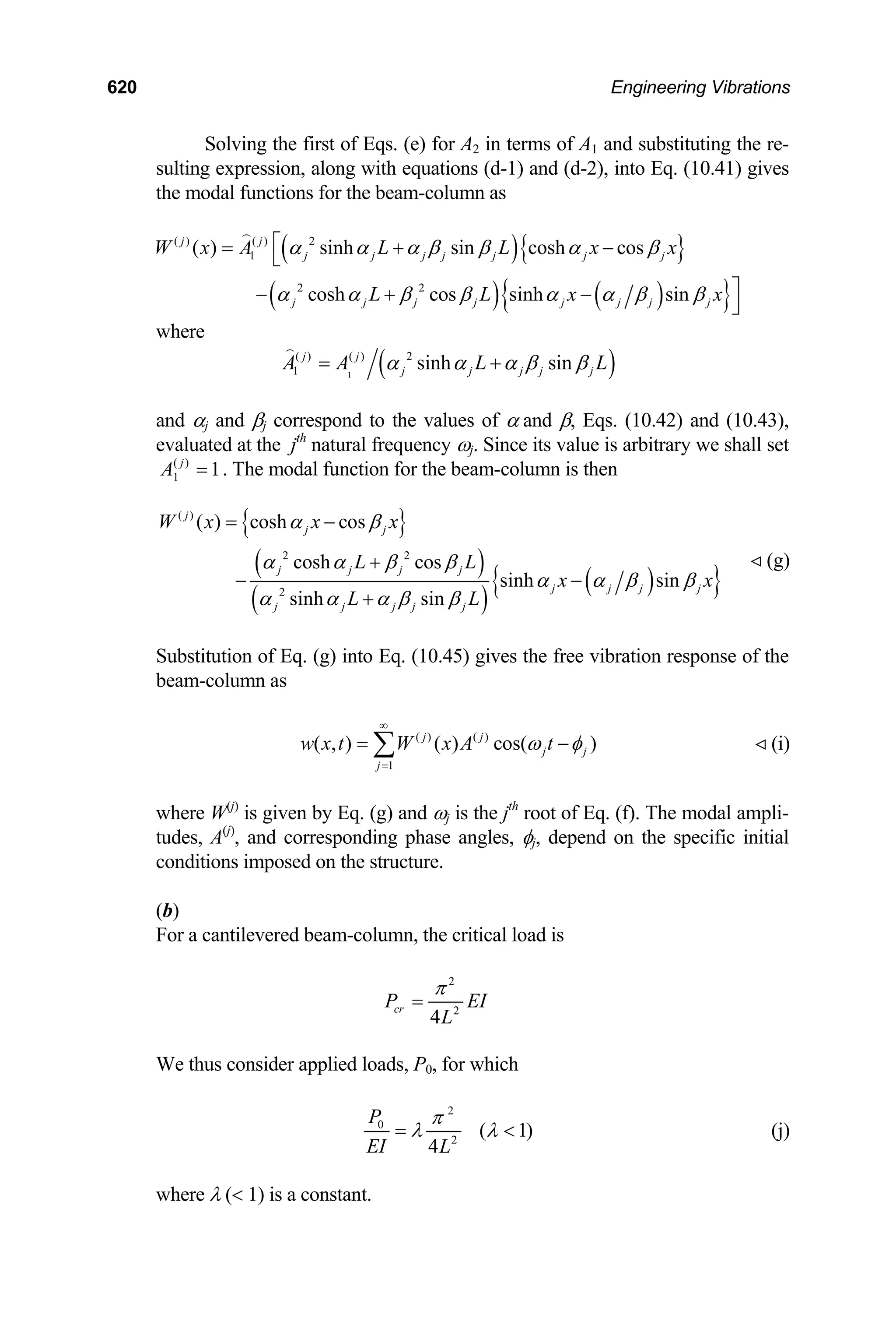
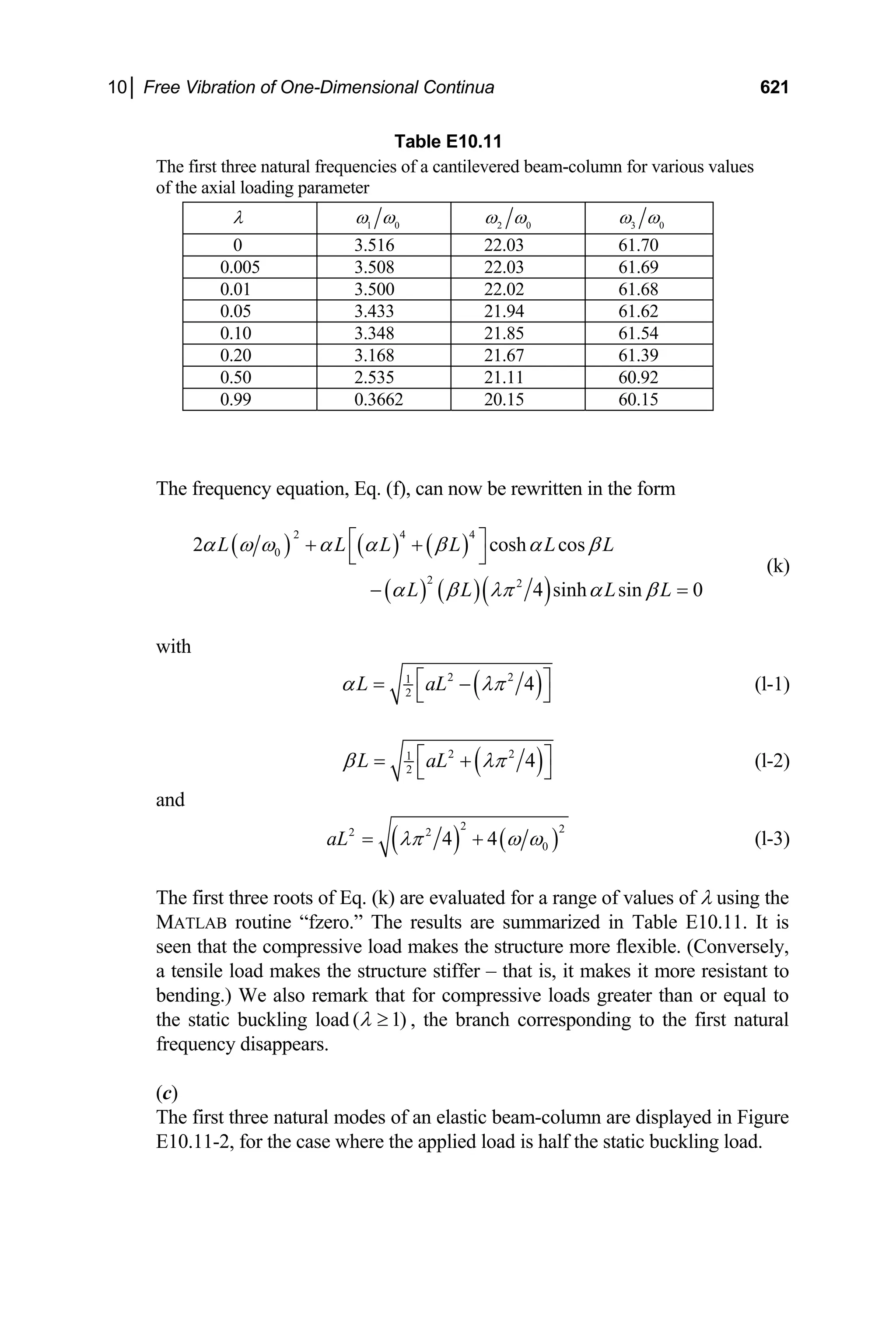
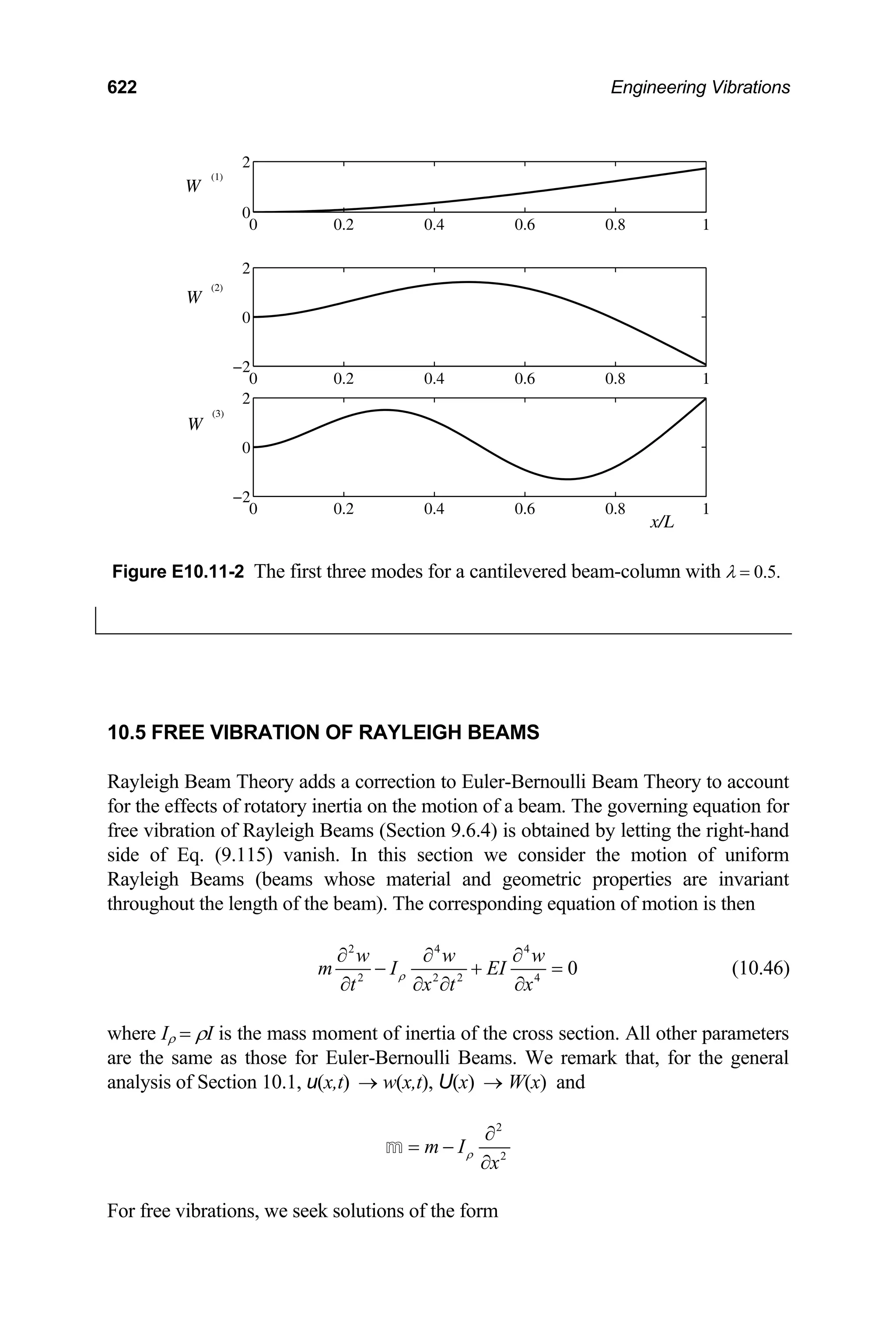
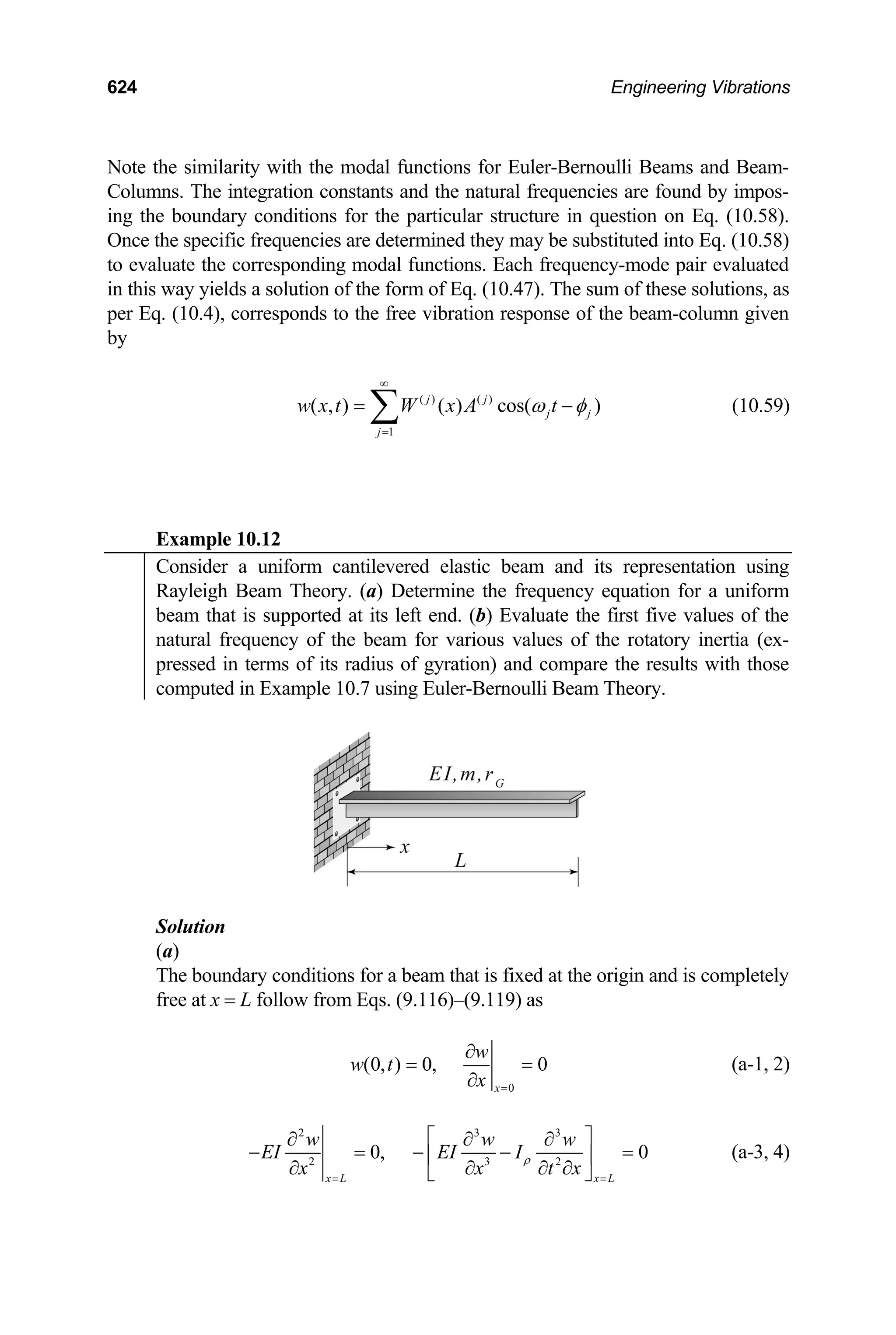
![10│ Free Vibration of One-Dimensional Continua 625
Substituting Eq. (10.47) into the above conditions gives the corresponding
boundary conditions for the modal functions,
(0) 0, (0) 0
W W′
= = (b-1, 2)
2
( ) 0, ( ) ( ) 0
W L W L W L
ϖ
′′ ′′′ ′
= + = (b-3, 4)
Note that since the rotatory inertia is included in the present model, the fre-
quency appears in the boundary condition for shear, Eq. (b-4), through the pa-
rameter ϖ. Imposing conditions (b-1)–(b-4) on Eq. (10.58) results in the system
of algebraic equations for the integration constants given by
1 3 0
A A
+ = (c-1)
2 4 0
A A
α β
+ = (c-2)
(c-3)
2 2 2 2
1 2 3 4
cosh sinh cos sin 0
A L A L A L A L
α α α α β β β β
+ − − =
[ ] [ ]
2 2
1 2 3 4
sinh cosh sin cos 0
A L A L A L A L
αβ α β α β β β
+ + − = (c-4)
The ensuing computations are simplified somewhat by substituting Eqs. (c-1)
and (c-2) into Eqs. (c-3) and (c-4) and writing the resulting equations in matrix
form as
2 2 2
1
2 2 2 3
2
0
( cosh cos ) ( sinh sin )
0
( sinh sin ) ( cosh cos )
A
L L L L
A
L L L L
α α β β α α αβ β
αβ α α β β αβ α α β
⎡ ⎤ ⎧ ⎫ ⎧ ⎫
+ +
=
⎨ ⎬ ⎨ ⎬
⎢ ⎥
− + ⎩ ⎭
⎩ ⎭
⎣ ⎦
(d)
For nontrivial solutions we require that the determinant of the matrix of coeffi-
cients in Eq. (d) vanish. This results in the frequency equation for the Rayleigh
Beam,
( )
2
4 4 2 2
2
2 cosh cos sinh sin 0
G
L L L L
r
ϖ
α α α β α β α βϖ α β
+ + − = (e)
Equation (e) may be solved numerically to obtain the set of natural frequencies
for the Rayleigh Beam. The modal function for the beam is then](https://image.slidesharecdn.com/engineeringvibrations-240713005818-b85f16c0/75/Engineering-Vibrations-Engineering-Vibrations-647-2048.jpg)
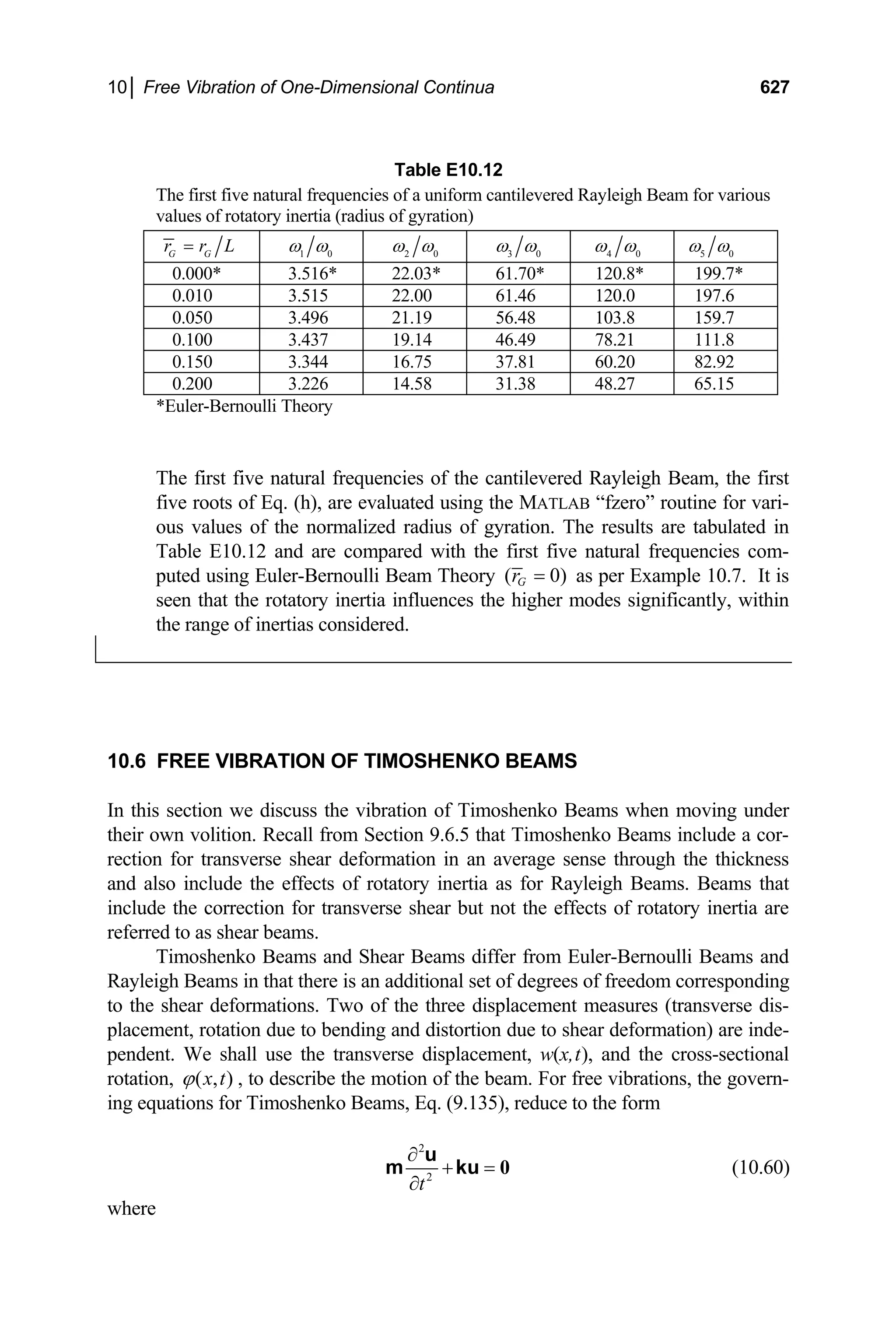
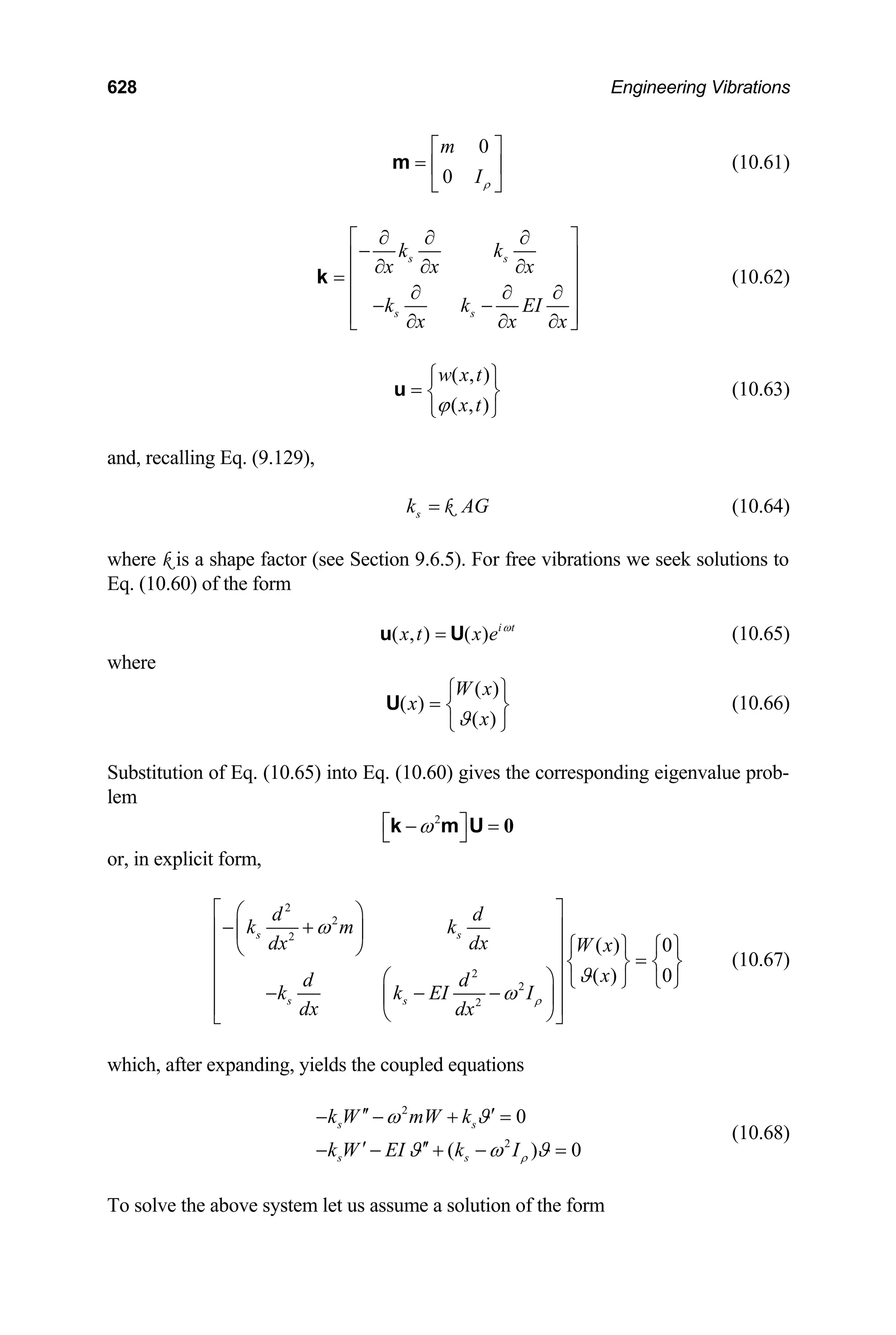
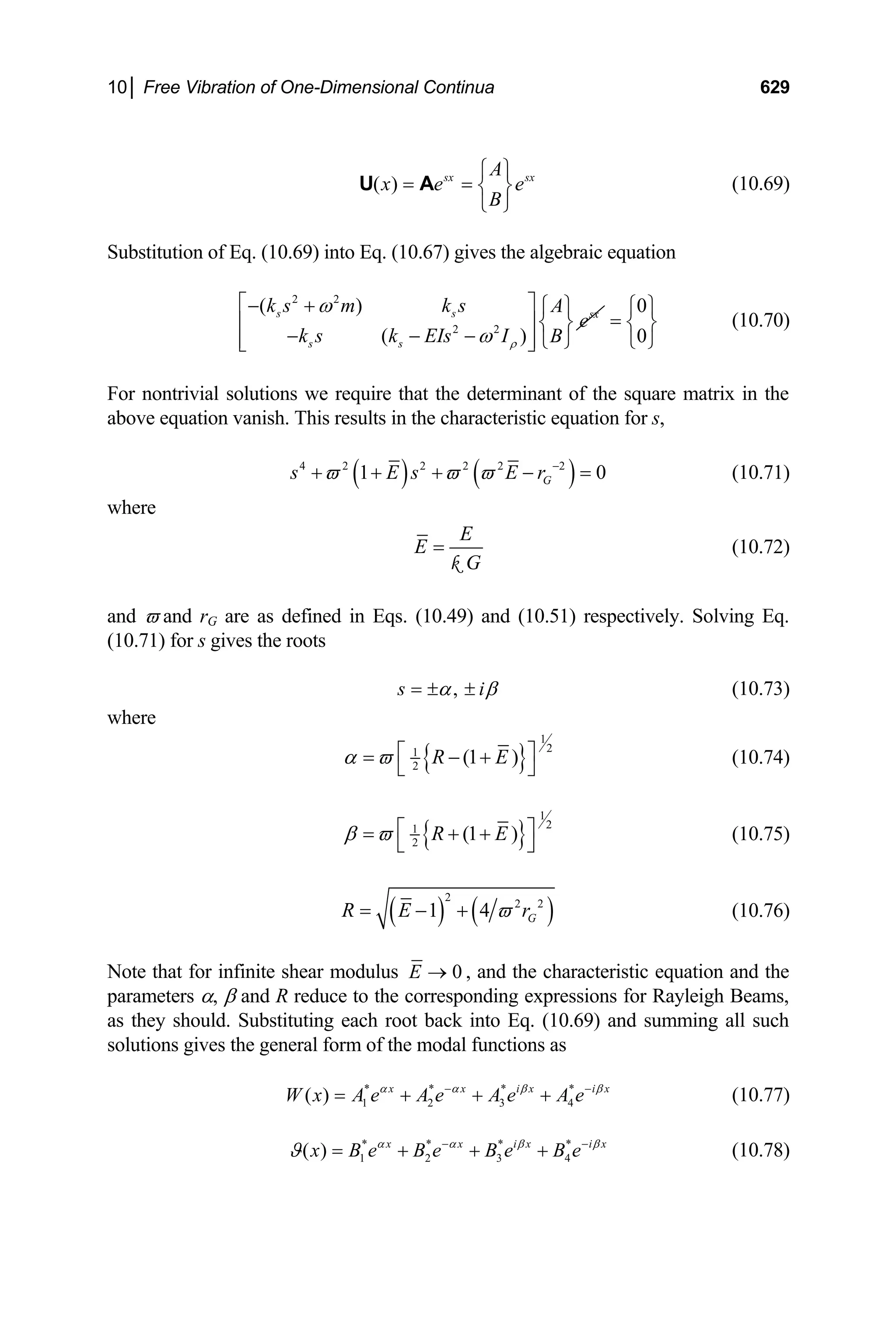
![630 Engineering Vibrations
The constants of integration of the modal rotation, ϑ(x), are related to the constants of
integration of the associated modal deflection, W(x), through Eq. (10.70). Since the
matrix of coefficients was rendered singular, both rows of that matrix equation yield
the same information. From the first row we find that
2
* E
B s A
s
ϖ
⎛
= +
⎜
⎝ ⎠
*
⎞
⎟ (10.79)
Evaluating Eq. (10.79) for each root of the characteristic equation for s gives the cor-
responding relations
2
*
1,2 1,2
E
B
ϖ
α
α
⎛ ⎞
= ± +
⎜ ⎟
⎝ ⎠
*
A (10.80)
and
2 2
* *
3,4 3,4 3,4
i
E E
B i A e A
π
ϖ ϖ
β β
β β
±
⎛ ⎞ ⎛ ⎞
= ± − = −
⎜ ⎟ ⎜ ⎟
⎝ ⎠ ⎝ ⎠
2 *
(10.81)
Substituting Eqs. (10.80) and (10.81) into Eq. (10.78) gives the modal rotation as
( )
( ) ( ) ( )
2 2 * *
1 2
2 2
2 2 * *
3 4
1
( )
1
x x
i x i x
x E A e A e
E A e A e
α α
β π β π
ϑ α ϖ
α
β ϖ
β
−
+ − +
⎡ ⎤
= + −
⎣ ⎦
⎡ ⎤
+ − +
⎣ ⎦
(10.82)
Using Eqs. (1.61) and (1.63) in Eqs. (10.77) and (10.82) renders the modal functions
to the forms
1 2 3 4
( ) cosh sinh cos sin
W x A x A x A x A x
α α β β
= + + + (10.83)
and
[ ] [ ]
1 2 3 4
( ) sinh cosh sin cos
x g A x A x g A x A x
α β
ϑ α α β
= + − − β (10.84)
where
( ) (
2 2 2 2
1 1
, )
g E g E
α β
α ϖ β ϖ
α β
= + = − (10.85)
and
( )
* * * * * * * *
1 1 2 2 1 2 3 3 4 4 3 4
, , ,
A A A A A A A A A A i A A
= + = − = + = − (10.86)
The remainder of the analysis proceeds as for the free vibration analysis of Euler-
Bernoulli Beams, etc. and depends upon the particular support conditions imposed on
the structure. Once the natural frequencies are obtained they are substituted into Eqs.
(10.83) and (10.84) for each mode. The general response is then found by substituting](https://image.slidesharecdn.com/engineeringvibrations-240713005818-b85f16c0/75/Engineering-Vibrations-Engineering-Vibrations-652-2048.jpg)
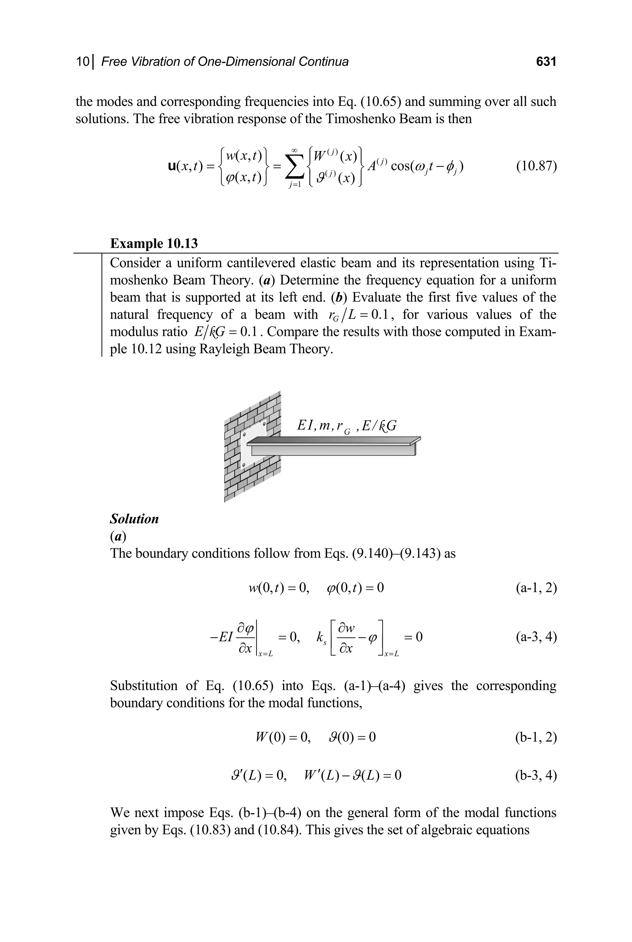
![632 Engineering Vibrations
1 3 0
A A
+ = (c-1)
2 4 0
g A g A
α β
+ = (c-2)
[ ] [ ]
1 2 3 4
cosh sinh cos sin 0
g A L A L g A L A L
α β
α α α β β β
+ − + = (c-3)
[ ] [ ]
1 2 3 4
( ) sinh cosh ( ) sin cos 0
g A L A L g A L A L
α β
α α α β β β
− + − − − = (c-4)
where gα and gβ are given by Eqs. (10.85). Substituting Eqs. (c-1) and (c-2) into
Eqs. (c-3) and (c-4) simplifies the calculation and gives two algebraic equations
in the two constants A1 and A2. The equations are expressed in matrix form as
11 12 1
21 22 2
0
0
H H A
H H A
⎡ ⎤ ⎧ ⎫ ⎧ ⎫
=
⎨ ⎬ ⎨ ⎬
⎢ ⎥
⎩ ⎭
⎣ ⎦ ⎩ ⎭
(d)
where
11 cosh cos
H g L g
α β L
α α β β
= + (e-1)
( )
12 sinh sin
H g L
α L
α α β β
= + (e-2)
21 ( )sinh ( )sin
H g L g
α β L
α α β β
= − + − (e-3)
22 ( )cosh ( )( )cos
H g L g g g
α β α β L
α α β β
= − − − (e-4)
Now, for nontrivial solutions the determinant of the matrix of coefficients of
Eq. (d) must vanish. This results in the frequency equation,
11 22 12 21
( ; ) 0
E H H H H
ϖ = −
F = (f)
which, after expanding, takes the form
( ) ( ) ( )
( )
2 2 2
1
cosh cos
2 sinh sin 0
g g E g g g g L L
g
g g g L
α β β α α β
β
α α β
ϖ β α α β α β
αβ β α α β
⎡ ⎤
− + + − − −
⎣ ⎦
⎡ ⎤ L
− − + =
⎣ ⎦
(f΄)
Equation (f) may be solved numerically for ϖ, for given material and geometric
parameters. Then, for each root ϖj (j = 1, 2, …) of the frequency equation, the
natural frequencies are found from Eq. (10.49) as
( 1,2,...)
j j a
c j
ω ϖ
= = (g)](https://image.slidesharecdn.com/engineeringvibrations-240713005818-b85f16c0/75/Engineering-Vibrations-Engineering-Vibrations-654-2048.jpg)
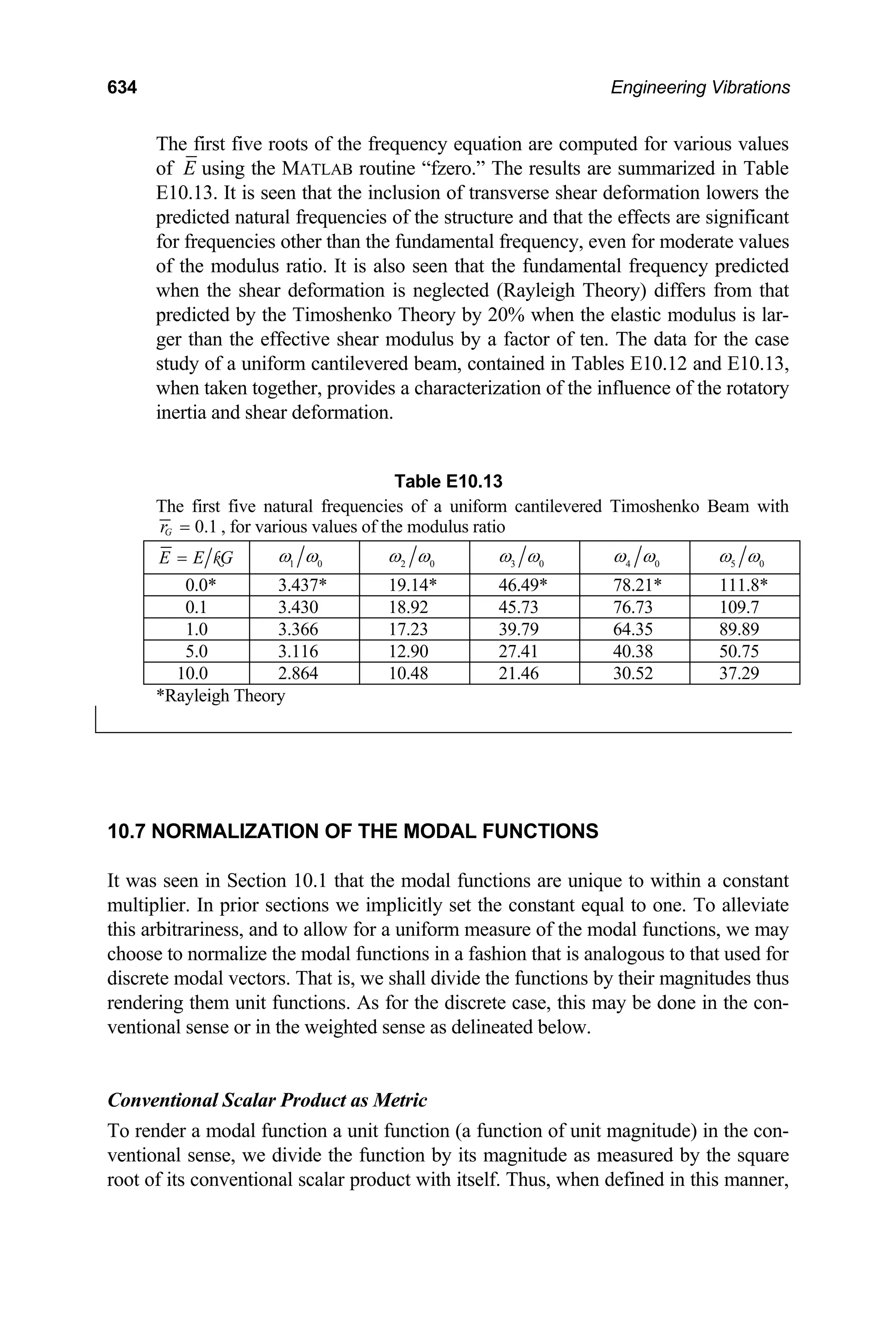
![10│ Free Vibration of One-Dimensional Continua 637
10.8.1 Systems Whose Mass Operators Are Scalar Functions
In this section we establish the general condition of orthogonality of the modal func-
tions for continuous systems whose mass operator corresponds to a single scalar
function of the spatial coordinate. These systems include the mathematical models for
longitudinal motion of elastic rods, torsional motion of elastic rods, transverse motion
of strings and cables, and transverse motion of Euler-Bernoulli Beams.
Systems Described by a Smooth Mass Distribution
To establish the conditions for the mutual orthogonality of the modal functions for
the class of systems under consideration we proceed in a fashion analogous to that
which was done in Section 7.3.2 for discrete systems.
It was seen in Section 10.1 that the general free-vibration problem is reduced to
finding the frequency-mode pairs that satisfy the eigenvalue problem defined by Eq.
(10.3). Let us consider the lth
and jth
natural frequencies and corresponding modal
functions
2 ( ) 2 ( )
, ( ) and , (
l j
l j )
x x
ω ω
U U
Each pair represents a solution to Eq. (10.3). Therefore
( ) 2 ( )
( ) ( )
l
l
l
x x
ω
=
U U
k m (10.92)
and
( ) 2 ( )
( ) ( )
j
j
j
x x
ω
=
U U
k m (10.93)
Let us multiply Eq. (10.92) by U(j)
(x)dx and Eq. (10.93) by U(l)
(x)dx. Integrating the
resulting expressions over [0, L] results in the identities
(10.94)
( ) ( ) 2 ( ) ( )
0 0
L L
j l j l
l
dx dx
ω
=
∫ ∫
U U U U
k m
m
and
(10.95)
( ) ( ) 2 ( ) ( )
0 0
L L
l j l j
j
dx dx
ω
=
∫ ∫
U U U U
k
Subtracting Eq. (10.95) from Eq. (10.94) gives
(10.96)
( ) ( ) ( ) ( )
0 0
2 ( ) ( ) 2 ( ) ( )
0 0
L L
j l l j
L L
j l l j
l j
dx dx
dx dx
ω ω
−
= −
∫ ∫
∫ ∫
U U U U
U U U U
k k
m m
where](https://image.slidesharecdn.com/engineeringvibrations-240713005818-b85f16c0/75/Engineering-Vibrations-Engineering-Vibrations-659-2048.jpg)
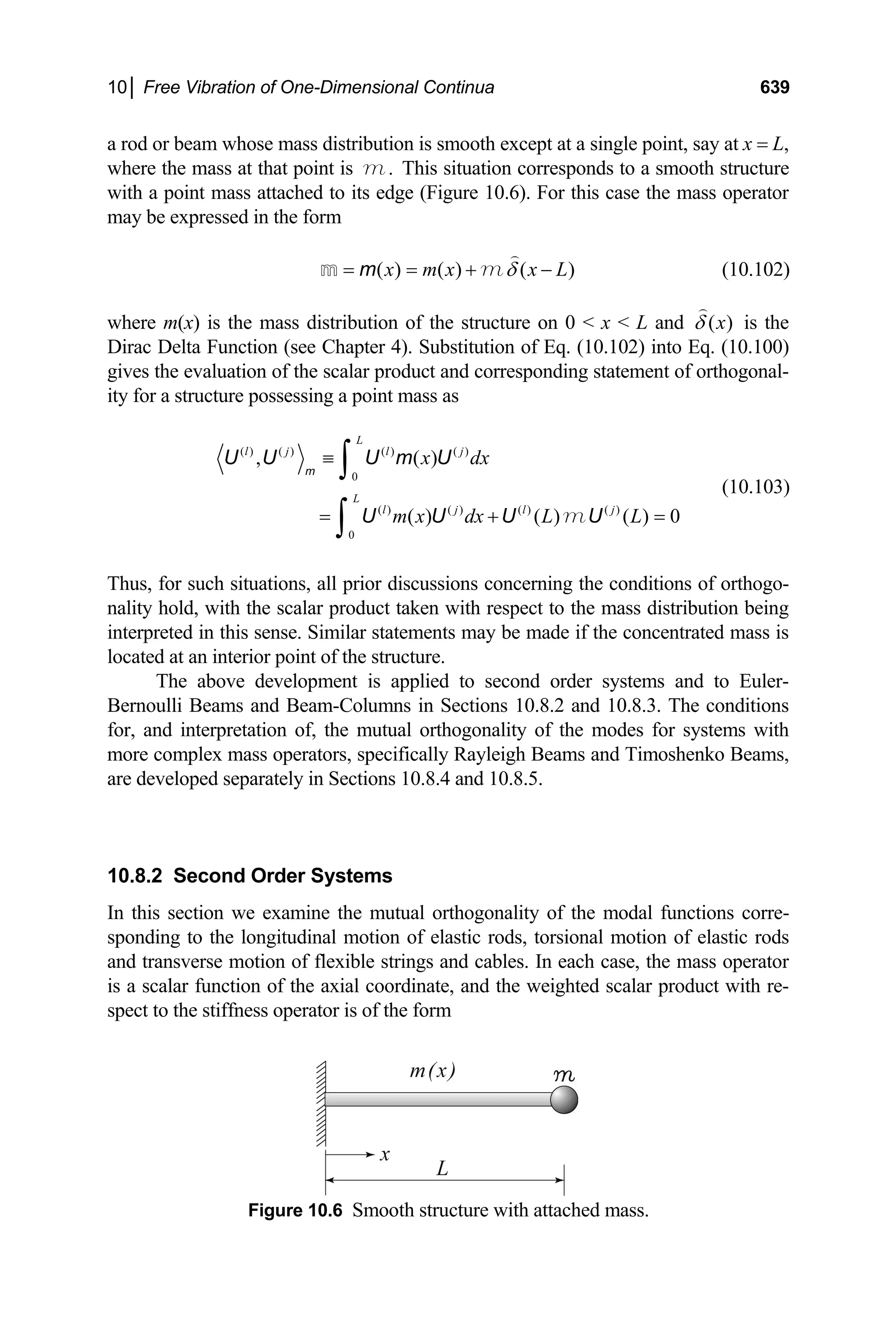
![642 Engineering Vibrations
the end of Section 10.8.1, then the mass operator and distribution is given by
Eq. (10.102). Viewing the structure in this sense, the boundary condition at the
right of the point mass (at x L+
= ) is then
( ) 0
N L+
=
(b)
The first bracketed expression of Eq. (10.111) is thus seen to vanish as well.
The modal functions are therefore mutually orthogonal with respect to the mass
in the sense of Eq. (10.103), and are therefore orthogonal with respect to the
stiffness operator in this sense as well.
Suppose, instead, that we had considered the rod and point mass as sepa-
rate structures. From Eq. (10.107) and Eq. (b) of Example 10.2, the boundary
condition at x = L−
is now
2 2
( ) ( ) ( ) ( )
a a
N L k U L k U L U L
m
β ω
′
= = =
m
m (c)
Substitution of Eqs. (a) and (c) into Eq. (10.111) results in the statement
2 2 ( ) ( )
( ) ( ) ( ) 0
j l
j l U L U L
ω ω
− =
m (d)
which is not generally satisfied if the tip mass is free to move. On this basis, we
might conclude that the modal functions are not mutually orthogonal. How-
ever, this simply means that the modal functions do not satisfy Eq. (10.100) on
the interval 0 x L−
. We would find, by direct calculation, that the modal
functions do satisfy Eq. (10.103) and are thus mutually orthogonal on the do-
main [0, L+
] in that sense.
Torsional Motion of Elastic Rods
For the case of torsional motion of rods, the vibration problem is described by the
angular displacement and the internal torque. We recall from Section 9.4 that, for
such motion, k = kT = GJ and m = Jρ. Thus, in the conditions for general and second
order systems described in Section 10.1 and at the beginning of this section, u(x,t)
θ(x,t), U(x) Θ(x), and m J
→ → → ρ = ρJ. Recall from Section 9.4 that the internal
torque, ( , )
x t
T , is related to the gradient of the angular displacement, ( , )
x t
θ , by the
relation
( , ) T
x t k GJ
x x
θ θ
∂ ∂
= =
∂ ∂
T (10.116)
Further, from earlier discussions, the free vibration response is of the general form](https://image.slidesharecdn.com/engineeringvibrations-240713005818-b85f16c0/75/Engineering-Vibrations-Engineering-Vibrations-664-2048.jpg)
![644 Engineering Vibrations
Example 10.16
Show that the modal functions corresponding to the system of Example 10.4
are mutually orthogonal.
Solution
From Eq. (a-1) of Example 10.4, the boundary condition at the elastic wall
gives
0
0 (0) (0)
i t i t
x
L L e
x
e
ω ω
θ
αθ α
=
∂
⎡ ⎤
′
− = = Θ − Θ
⎢ ⎥
∂
⎣ ⎦
The corresponding modal boundary condition at the left end of the rod is thus
(0) (0)
L α
′
Θ = Θ (a)
From condition (a-2) of Example 10.4, the boundary condition arising from the
presence of the rigid wall at the right end of the rod follows as
( , ) 0 ( ) ( ) 0
i t
L t L e L
ω
θ = = Θ ⇒ Θ = (b)
Substituting Eq. (a) into Eq. (10.119) gives the relation
( ) ( )
(0) (0)
j j
T
k L
α
= Θ
T (c)
Finally, substituting of Eqs. (b) and (c) into the left hand side of Eq. (10.120)
gives
[ ] ( ) ( ) ( ) ( ) ( )
0 0 (0) (0) (0) (0) 0
j i i j
T
k L
α ⎡
− − Θ Θ − Θ Θ =
⎣ ⎤
⎦ (d)
It is seen that Eq. (10.120) is satisfied, and thus that the modal functions are
mutually orthogonal with respect to both m and k.
Transverse Motion of Strings and Cables
When considering the transverse motion of flexible strings and cables, the motion is
characterized by the transverse displacement and the mass by the mass per unit
length. Hence, for these systems, u(x,t) w(x,t), U(x) W(x) and m = m(x) in the
general statements of Section 10.1. We also recall from Section 9.5 that the trans-
verse shear force, Q, is related to the displacement gradient by the relation
→ →](https://image.slidesharecdn.com/engineeringvibrations-240713005818-b85f16c0/75/Engineering-Vibrations-Engineering-Vibrations-666-2048.jpg)