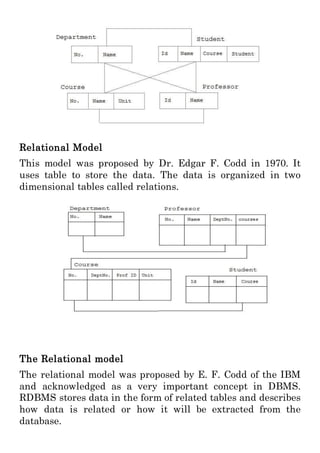
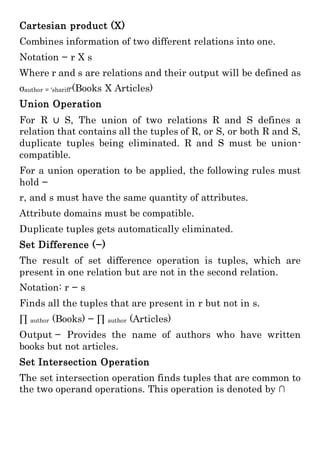
1. Overview of Database
A Database is a collection of logically related data stored in a
particular manner, from which information/data can be easily
accessed, managed and updated at a very fast speed.
An electronic data processing system that uses a database for
the storage of data is known as a database system.
Example: Payroll Management System, Banking, Booking
Tickets.
Database Management System (DBMS)
A DBMS is a software that allows creation, definition and
manipulation of database. DBMS is actually a tool used to
perform any kind of operation on data in database. DBMS also
provides protection and security to database. It maintains
data consistency in case of multiple users. Here are some
EDP is referred to the use of automated
methods to process commercial data.
2. examples of popular DBMS, MySQL, Oracle, Microsoft Access
and IBM DB2 etc.
Advantages of DBMS
Reduced data redundancy (duplicacy of data)
Data independence and consistency
Easy retrieval of data
Information protection (data integrity & security)
Components of database system
Users - Users may be of various type such as DB
administrator, System developer and End users.
Database application - Database application may be Personal,
Enterprise and Internal.
DBMS - Software that allow users to define, create and
manages database access, Ex: MySQL, Oracle etc.
Database - Collection of logical data.
3. Purposes of Databases
- Databases reduce the data redundancy to a large extent.
- Databases can control data inconsistency to a large extent.
- Databases facilitate sharing of data.
- Databases can ensure data security
- Data integrity can be maintained through databases
Database Abstraction
Data Abstraction is a process of hiding irrelevant details from
user. The major purpose is to provide only that much
information that is required by them.
Various levels of database implementation
Physical Level: In this level it describes how data are actually
stored on the storage medium. You can get the complex data
structure details at this level.
Conceptual Level: In this level it describes what data are
actually stored and also describes the relationships among
data.
View Level: In this level it describes only the information from
the database which is required by the individual user.
Concept of data independence
The ability to modify a scheme definition in one level without
effecting a scheme definition in the next level is called Data
Independence.
Physical data independence refers to the ability to modify the
scheme followed at the physical level without affecting the
scheme followed at conceptual level.
4. Logical data independence refers to the ability to modify the
conceptual scheme without causing any changes in the scheme
followed at view levels.
Different Data models
A Data model is a collection of concepts that can be used to
describe the structure of a database, including the
relationships and constraints that determine how data can be
stored and accessed.
Three models are commonly used. They are,
Hierarchical Model
The hierarchical model organizes data into a tree-like
structure, where each record has a single parent or root.
Sibling records are sorted in a particular order. That order is
used as the physical order for storing the database. This model
is good for describing many real-world relationships.
Network Model
This data model represents many to many relationship. It is
represented by collection of records and relationships among
data are represented as links.
5. Relational Model
This model was proposed by Dr. Edgar F. Codd in 1970. It
uses table to store the data. The data is organized in two
dimensional tables called relations.
The Relational model
The relational model was proposed by E. F. Codd of the IBM
and acknowledged as a very important concept in DBMS.
RDBMS stores data in the form of related tables and describes
how data is related or how it will be extracted from the
database.
6. Entity - An Entity is an object which can be distinctly
identified.
Relation - A relation is similar to table which consists of rows
and columns. It is the basic storage structure of RDBMS.
Domain - The domain is a set of possible values that an
attribute can have.
Tuple - A row in a relation is also called as a tuple.
Attribute - a column in a relation is also called as an attribute.
Degree - The number of attributes in a relation is called the
degree of the relation.
Cardinality - The number of tuples in a relation is called the
cardinality of that relation.
Views - A view is a kind of table whose contents are taken
from other tables depending upon a condition. The contents of
a view are determined by carrying out the execution of the
given query.
Structure of Relational Databases
Keys - Keys are used to establish and identify relations
between tables. They also ensure that each record within a
table can be uniquely identified by combination of one or more
attributes within a table.
Primary key
A primary key is a set of one or more attributes that can
uniquely identify tuples within the relation.
7. Candidate key
Candidate keys are defined as the set of fields from which
primary key can be selected. It is an attribute or set of
attribute that can act as a primary key for a table to uniquely
identify each record in that table.
8. Alternate key
The candidate key which are not selected for primary key are
known as alternative keys
Let's take an example of student it can contain NAME, ROLL
NO., ID and CLASS.
Here ROLL NO. is primary key and rest of all columns like
NAME, ID and CLASS are alternate keys.
If a table has more than one candidate key, one of them will
become the primary key and rest of all are called alternate
keys.
Foreign key
A FOREIGN KEY is a key used to link two tables together.
A FOREIGN KEY is a field (or collection of fields) in one table
that refers to the PRIMARY KEY in another table.
The table containing the foreign key is called the child table,
and the table containing the candidate key is called the
referenced or parent table.
9. The Relation Algebra
Select Operation (σ)
It selects tuples that satisfy the given predicate from a
relation.
Notation − σp(r)
Where σ stands for selection predicate and r stands for
relation. p is prepositional logic formula which may use
connectors like and, or, and not. These terms may use
relational operators like − =, ≠, ≥, <, >, ≤.
For example −
σsubject = "Computer Science"(Books)
Output − Selects tuples from books where subject is 'Computer
Science'.
σsubject = "maths" and price = "450"(Books)
Output − Selects tuples from books where subject is 'maths'
and 'price' is 450.
Project Operation (∏)
It projects column(s) that satisfy a given predicate.
Notation − ∏A1, A2, An (r)
Where A1, A2, are attribute names of relation r.
Duplicate rows are automatically eliminated, as relation is a
set.
For example −
∏subject, author (Books)
Selects and projects columns named as subject and author
from the relation Books.
10. Cartesian product (Χ)
Combines information of two different relations into one.
Notation − r Χ s
Where r and s are relations and their output will be defined as
σauthor = 'shariff'(Books Χ Articles)
Union Operation
For R ∪ S, The union of two relations R and S defines a
relation that contains all the tuples of R, or S, or both R and S,
duplicate tuples being eliminated. R and S must be union-
compatible.
For a union operation to be applied, the following rules must
hold −
r, and s must have the same quantity of attributes.
Attribute domains must be compatible.
Duplicate tuples gets automatically eliminated.
Set Difference (−)
The result of set difference operation is tuples, which are
present in one relation but are not in the second relation.
Notation: r − s
Finds all the tuples that are present in r but not in s.
∏ author (Books) − ∏ author (Articles)
Output − Provides the name of authors who have written
books but not articles.
Set Intersection Operation
The set intersection operation finds tuples that are common to
the two operand operations. This operation is denoted by ∩