![MATLAB commands in numerical Python 2
Vidar Bronken Gundersen /mathesaurus.sf.net
List available packages
matlab help
R library()
Python help(); modules [Numeric]
Locate functions
matlab which plot
Scilab whereis plot
R find(plot)
Python help(plot)
List available methods for a function
R methods(plot)
1.2 Using interactively
Start session
Octave octave -q
R Rgui
Python ipython -pylab
idl idlde
bc bc -lq
gnuplot pgnuplot
Auto completion
Octave TAB or M-?
Scilab ! // commands in history
Python TAB
Run code from file
matlab foo(.m)
Scilab exec(’foo.sce’)
R source(’foo.R’)
Python execfile(’foo.py’) or run foo.py
gnuplot load ’foo.gp’
idl @"foo.idlbatch" or .run ’foo.pro’
Maxima batch("foo.mc")
Command history
Octave history
Scilab gethistory
R history()
Python hist -n
idl help,/rec
Axiom )history )show
Save command history
matlab diary on [..] diary off
Scilab diary(’session.txt’) [..] diary(0)
R savehistory(file=".Rhistory")
idl journal,’IDLhistory’
Axiom )hist )write foo.input
End session
matlab exit or quit
R q(save=’no’)
Python CTRL-D
CTRL-Z # windows
sys.exit()
gnuplot exit or quit
idl exit or CTRL-D
Axiom )quit
Maxima quit();
Maple quit
Mathematica Quit[]
MuPAD quit
Derive [Quit]
reduce quit;
bc quit
2 Operators
Help on operator syntax
matlab help -
Scilab help symbols
R help(Syntax)
2.1 Arithmetic operators
Assignment; defining a number
matlab a=1; b=2;
R a<-1; b<-2
Python a=1; b=1
idl a=1 & b=1
bc a=1; b=1](https://image.slidesharecdn.com/math-synonyms-120226112112-phpapp01/85/Math-synonyms-2-320.jpg)
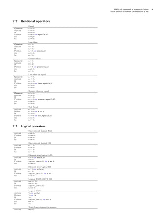
![MATLAB commands in numerical Python 3
Vidar Bronken Gundersen /mathesaurus.sf.net
Addition
Generic a + b
matlab a + b
R a + b
Python a + b or add(a,b)
gnuplot a + b
idl a + b
bc a + b
Subtraction
Generic a - b
matlab a - b
R a - b
Python a - b or subtract(a,b)
gnuplot a - b
idl a - b
bc a - b
Multiplication
Generic a * b
matlab a * b
R a * b
Python a * b or multiply(a,b)
gnuplot a * b
idl a * b
bc a * b
Division
Generic a / b
matlab a / b
R a / b
Python a / b or divide(a,b)
gnuplot a / b
idl a / b
Power, ab
matlab a .^ b
R a ^ b
Python a ** b
power(a,b)
pow(a,b)
gnuplot a ** b
idl a ^ b
Axiom a**b
Maxima a^b or a**b
bc a ^ b
Remainder
matlab rem(a,b)
Scilab modulo(a,b)
R a %% b
Python a % b
remainder(a,b)
fmod(a,b)
gnuplot a % b
idl a MOD b
Axiom rem(a,b)
Maxima mod(a,b)
Maple a mod b
Mathematica Mod[a,b]
MuPAD a mod b
Derive MOD(a,b)
bc a % b
Integer division
R a %/% b
bc a / b
Increment, return new value
Octave ++a
idl ++a or a+=1
bc ++a
Increment, return old value
Octave a++
idl a++
bc a++
In place operation to save array creation overhead
Python a+=b or add(a,b,a)
Octave a+=1
idl a+=1
bc a+=b
Factorial, n!
matlab factorial(a)
R factorial(a)
Axiom factorial(a)
Maxima a!
Maple a!](https://image.slidesharecdn.com/math-synonyms-120226112112-phpapp01/85/Math-synonyms-3-320.jpg)
![MATLAB commands in numerical Python 5
Vidar Bronken Gundersen /mathesaurus.sf.net
True if all elements are nonzero
matlab all(a)
Scilab and(a)
2.4 root and logarithm
Square root
Generic sqrt(a)
matlab sqrt(a)
R sqrt(a)
Python math.sqrt(a)
gnuplot sqrt(a) √
a
idl sqrt(a)
Axiom sqrt(a)
Maxima sqrt(a)
Maple sqrt(a)
Mathematica Sqrt[a]
bc sqrt(a)
Logarithm, base e (natural)
Generic log(a)
matlab log(a)
R log(a)
Python math.log(a)
gnuplot log(a)
idl alog(a) ln a = loge a
Axiom log(a)
Maxima log(a)
Maple log(a)
Mathematica Log[a]
MuPAD ln(a)
bc l(a)
Logarithm, base
Generic log10(a)
matlab log10(a)
R log10(a) log10 a
Python math.log10(a)
gnuplot log10(a)
idl alog10(a)
Logarithm, base (binary)
matlab log2(a)
log2 a
R log2(a)
Python math.log(a, 2)
Exponential function
Generic exp(a)
matlab exp(a)
R exp(a)
ea
Python math.exp(a)
gnuplot exp(a)
idl exp(a)
bc e(a)
2.5 Round off
Round
matlab round(a)
R round(a)
Python around(a) or math.round(a)
idl round(a)
Round up
matlab ceil(a)
R ceil(a)
Python ceil(a)
gnuplot ceil(a)
idl ceil(a)
Round down
matlab floor(a)
R floor(a)
Python floor(a)
gnuplot floor(a)
idl floor(a)
Round towards zero
matlab fix(a)
Python fix(a)](https://image.slidesharecdn.com/math-synonyms-120226112112-phpapp01/85/Math-synonyms-5-320.jpg)

![MATLAB commands in numerical Python 7
Vidar Bronken Gundersen /mathesaurus.sf.net
Imaginary part
Generic imag(z)
matlab imag(z)
R Im(3+4i)
Python z.imag
idl imaginary(z)
gnuplot imag({3,4})
Maxima imagpart(z)
Argument
matlab arg(z)
R Arg(3+4i)
gnuplot arg({3,4})
Complex conjugate
Generic conj(z)
matlab conj(z)
R Conj(3+4i)
Python z.conj(); z.conjugate()
idl conj(z)
2.8 Trigonometry
Sine
Generic sin(a)
Cosine
Generic cos(a)
Tangent
Generic tan(a)
Arcsine
Generic asin(a) or arcsin(a)
Arccosine
Generic acos(a) or arccos(a)
Arctangent
Generic atan(a) or arctan(a)
Arctangent, arctan(b/a)
matlab atan(a,b)
R atan2(b,a)
Python atan2(b,a)
Hyperbolic sine
Generic sinh(a)
Hyperbolic cosine
Generic cosh(a)
Hyperbolic tangent
Generic tanh(a)
Hypotenus; Euclidean distance
x2 + y 2
Python hypot(x,y)
2.9 Generate random numbers
Uniform distribution
matlab rand(1,10)
Scilab rand(1,10,’uniform’)
R runif(10)
Python random.random((10,))
random.uniform((10,))
idl randomu(seed, 10)
Uniform: Numbers between and
matlab 2+5*rand(1,10)
Scilab 2+5*rand(1,10,’uniform’)
R runif(10, min=2, max=7)
Python random.uniform(2,7,(10,))
idl 2+5*randomu(seed, 10)
Uniform: , array
matlab rand(6)
Scilab rand(6,6,’uniform’)
R matrix(runif(36),6)
Python random.uniform(0,1,(6,6))
idl randomu(seed,[6,6])
Normal distribution
matlab randn(1,10)
Scilab rand(1,10,’normal’)
R rnorm(10)
Python random.standard_normal((10,))
idl randomn(seed, 10)](https://image.slidesharecdn.com/math-synonyms-120226112112-phpapp01/85/Math-synonyms-7-320.jpg)
![MATLAB commands in numerical Python 8
Vidar Bronken Gundersen /mathesaurus.sf.net
3 Vectors
Row vector, 1 × n-matrix
matlab a=[2 3 4 5];
R a <- c(2,3,4,5)
Python a=array([2,3,4,5])
idl a = [2, 3, 4, 5]
Column vector, m × 1-matrix
matlab adash=[2 3 4 5]’;
R adash <- t(c(2,3,4,5))
Python array([2,3,4,5])[:,NewAxis]
array([2,3,4,5]).reshape(-1,1)
r_[1:10,’c’]
idl transpose([2,3,4,5])
3.1 Sequences
,,, ... ,
matlab 1:10
R seq(10) or 1:10
Python arange(1,11, dtype=Float)
range(1,11)
idl indgen(10)+1
dindgen(10)+1
.,.,., ... ,.
matlab 0:9
R seq(0,length=10)
Python arange(10.)
idl dindgen(10)
,,,
matlab 1:3:10
R seq(1,10,by=3)
Python arange(1,11,3)
idl indgen(4)*3+1
,,, ... ,
matlab 10:-1:1
R seq(10,1) or 10:1
Python arange(10,0,-1)
,,,
matlab 10:-3:1
R seq(from=10,to=1,by=-3)
Python arange(10,0,-3)
Linearly spaced vector of n= points
matlab linspace(1,10,7)
R seq(1,10,length=7)
Python linspace(1,10,7)
Reverse
matlab reverse(a)
Scilab a($:-1:1)
R rev(a)
Python a[::-1] or
idl reverse(a)
Set all values to same scalar value
matlab a(:) = 3
Python a.fill(3), a[:] = 3
3.2 Concatenation (vectors)
Concatenate two vectors
matlab [a a]
R c(a,a)
Python concatenate((a,a))
idl [a,a] or rebin(a,2,size(a))
matlab [1:4 a]
R c(1:4,a)
Python concatenate((range(1,5),a), axis=1)
idl [indgen(3)+1,a]
3.3 Repeating
,
matlab [a a]
R rep(a,times=2)
Python concatenate((a,a))
, ,
R rep(a,each=3)
Python a.repeat(3) or](https://image.slidesharecdn.com/math-synonyms-120226112112-phpapp01/85/Math-synonyms-8-320.jpg)
![MATLAB commands in numerical Python 9
Vidar Bronken Gundersen /mathesaurus.sf.net
, ,
R rep(a,a)
Python a.repeat(a) or
3.4 Miss those elements out
miss the first element
matlab a(2:end)
Scilab a(2:$)
R a[-1]
Python a[1:]
miss the tenth element
matlab a([1:9])
R a[-10]
miss ,,, ...
R a[-seq(1,50,3)]
last element
matlab a(end)
Scilab a($)
Python a[-1]
last two elements
matlab a(end-1:end)
Python a[-2:]
3.5 Maximum and minimum
pairwise max
matlab max(a,b)
Python maximum(a,b)
R pmax(a,b)
max of all values in two vectors
matlab max([a b])
Python concatenate((a,b)).max()
R max(a,b)
matlab [v,i] = max(a)
Python v,i = a.max(0),a.argmax(0)
R v <- max(a) ; i <- which.max(a)
3.6 Vector multiplication
Multiply two vectors
matlab a.*a
R a*a
Python a*a
Vector cross product, u × v
idl crossp(u,v)
Mathematica cross(u,v)
Vector dot product, u · v
matlab dot(u,v)
Python dot(u,v)
4 Matrices
Define a matrix
matlab a = [2 3;4 5]
R rbind(c(2,3),c(4,5))
array(c(2,3,4,5), dim=c(2,2))
Python a = array([[2,3],[4,5]])
2 3
idl a = [[2,3],[4,5]]
4 5
Axiom a := matrix [[2,3],[4,5]]
Maxima matrix([2,3],[4,5])
Maple matrix([[2,3],[4,5]])
Mathematica {{2,3},{4,5}}
Derive [[2,3],[4,5]]
4.1 Concatenation (matrices); rbind and cbind
Bind rows
matlab [a ; b]
R rbind(a,b)
Python concatenate((a,b), axis=0)
vstack((a,b))
Bind columns
matlab [a , b]
R cbind(a,b)
Python concatenate((a,b), axis=1)
hstack((a,b))](https://image.slidesharecdn.com/math-synonyms-120226112112-phpapp01/85/Math-synonyms-9-320.jpg)
![MATLAB commands in numerical Python 10
Vidar Bronken Gundersen /mathesaurus.sf.net
Bind slices (three-way arrays)
Python concatenate((a,b), axis=2)
dstack((a,b))
Concatenate matrices into one vector
matlab [a(:), b(:)]
Python concatenate((a,b), axis=None)
Bind rows (from vectors)
matlab [1:4 ; 1:4]
R rbind(1:4,1:4)
Python concatenate((r_[1:5],r_[1:5])).reshape(2,-1)
vstack((r_[1:5],r_[1:5]))
[,1] [,2] [,3] [,4]
[1,] 1 2 3 4
[2,] 1 2 3 4
Bind columns (from vectors)
matlab [1:4 ; 1:4]’
R cbind(1:4,1:4)
[,1] [,2]
[1,] 1 1
[2,] 2 2
[3,] 3 3
[4,] 4 4
4.2 Array creation
filled array
matlab zeros(3,5) 0 0 0 0 0
R matrix(0,3,5) or array(0,c(3,5)) 0 0 0 0 0
Python zeros((3,5),Float) 0 0 0 0 0
idl dblarr(3,5)
filled array of integers
Python zeros((3,5))
idl intarr(3,5)
filled array
matlab ones(3,5) 1 1 1 1 1
R matrix(1,3,5) or array(1,c(3,5)) 1 1 1 1 1
Python ones((3,5),Float) 1 1 1 1 1
idl dblarr(3,5)+1
Any number filled array
matlab ones(3,5)*9 9 9 9 9 9
R matrix(9,3,5) or array(9,c(3,5)) 9 9 9 9 9
Python 9 9 9 9 9
idl intarr(3,5)+9
Identity matrix
matlab eye(3)
1 0 0
Scilab eye(3,3)
0 1 0
R diag(1,3)
0 0 1
Python identity(3)
idl identity(3)
Diagonal
matlab diag([4 5 6])
4 0 0
R diag(c(4,5,6))
0 5 0
Python diag((4,5,6))
0 0 6
idl diag_matrix([4,5,6])
Axiom diagonalMatrix([4,5,6])
Magic squares; Lo Shu 8 1 6
matlab magic(3) 3 5 7
Scilab testmatrix(’magi’,3) 4 9 2
Empty array
Python a = empty((3,3))
4.3 Reshape and flatten matrices
Reshaping (rows first)
matlab reshape(1:6,3,2)’;
Scilab matrix(1:6,3,2)’;
1 2 3
R matrix(1:6,nrow=3,byrow=T)
4 5 6
Python arange(1,7).reshape(2,-1)
a.setshape(2,3)
idl reform(a,2,3)
Reshaping (columns first)
matlab reshape(1:6,2,3);
Scilab matrix(1:6,2,3); 1 3 5
R matrix(1:6,nrow=2) 2 4 6
array(1:6,c(2,3))
Python arange(1,7).reshape(-1,2).transpose()
Flatten to vector (by rows, like comics)
matlab a’(:)
1 2 3 4 5 6
R as.vector(t(a))
Python a.flatten() or](https://image.slidesharecdn.com/math-synonyms-120226112112-phpapp01/85/Math-synonyms-10-320.jpg)
![MATLAB commands in numerical Python 11
Vidar Bronken Gundersen /mathesaurus.sf.net
Flatten to vector (by columns)
matlab a(:)
R as.vector(a) 1 4 2 5 3 6
Python a.flatten(1)
Flatten upper triangle (by columns)
matlab vech(a)
R a[row(a) <= col(a)]
4.4 Shared data (slicing)
Copy of a
matlab b = a
R b = a
Python b = a.copy()
4.5 Indexing and accessing elements (Python: slicing)
Input is a , array
matlab a = [ 11 12 13 14 ...
21 22 23 24 ...
31 32 33 34 ]
R a <- rbind(c(11, 12, 13, 14),
c(21, 22, 23, 24), a11 a12 a13 a14
c(31, 32, 33, 34)) a21 a22 a23 a24
Python a = array([[ 11, 12, 13, 14 ], a31 a32 a33 a34
[ 21, 22, 23, 24 ],
[ 31, 32, 33, 34 ]])
idl a = [[ 11, 12, 13, 14 ], $
[ 21, 22, 23, 24 ], $
[ 31, 32, 33, 34 ]]
Element , (row,col)
matlab a(2,3)
R a[2,3] a23
Python a[1,2]
idl a(2,1)
First row
matlab a(1,:)
R a[1,] a11 a12 a13 a14
Python a[0,]
idl a(*,0)
First column
matlab a(:,1) a11
R a[,1] a21
Python a[:,0] a31
idl a(0,*)
Array as indices
matlab a([1 3],[1 4]); a11 a14
Python a.take([0,2]).take([0,3], axis=1) a31 a34
All, except first row
matlab a(2:end,:)
Scilab a(2:$,:) a21 a22 a23 a24
R a[-1,] a31 a32 a33 a34
Python a[1:,]
idl a(*,1:*)
Last two rows
a21 a22 a23 a24
matlab a(end-1:end,:)
a31 a32 a33 a34
Python a[-2:,]
Strides: Every other row
a11 a12 a13 a14
matlab a(1:2:end,:)
a31 a32 a33 a34
Python a[::2,:]
Third in last dimension (axis)
Python a[...,2]
All, except row,column (,) a11 a13 a14
R a[-2,-3] a31 a33 a34
Remove one column
matlab a(:,[1 3 4]) a11 a13 a14
R a[,-2] a21 a23 a24
Python a.take([0,2,3],axis=1) a31 a33 a34
Diagonal
a11 a22 a33 a44
Python a.diagonal(offset=0)
4.6 Assignment
matlab a(:,1) = 99
R a[,1] <- 99
Python a[:,0] = 99](https://image.slidesharecdn.com/math-synonyms-120226112112-phpapp01/85/Math-synonyms-11-320.jpg)
![MATLAB commands in numerical Python 12
Vidar Bronken Gundersen /mathesaurus.sf.net
matlab a(:,1) = [99 98 97]’
R a[,1] <- c(99,98,97)
Python a[:,0] = array([99,98,97])
Clipping: Replace all elements over
matlab a(a>90) = 90;
R a[a>90] <- 90
Python (a>90).choose(a,90)
a.clip(min=None, max=90)
idl a>90
Clip upper and lower values
Python a.clip(min=2, max=5)
idl a < 2 > 5
4.7 Transpose and inverse
Transpose
matlab a’
R t(a)
Python a.conj().transpose()
idl transpose(a)
Maxima transpose(a);
Non-conjugate transpose
matlab a.’ or transpose(a)
Python a.transpose()
Determinant
matlab det(a)
R det(a)
Python linalg.det(a) or determinant(a)
idl determ(a)
Axiom determinant a
Maxima determinant(a);
Inverse
matlab inv(a)
R solve(a)
Python linalg.inv(a) or inverse(a)
idl invert(a)
Axiom inverse a
Maxima invert(a),detout;
Pseudo-inverse
matlab pinv(a)
R ginv(a)
Python linalg.pinv(a)
Norms
matlab norm(a)
Python norm(a)
Eigenvalues
matlab eig(a)
Scilab spec(a)
R eigen(a)$values
Python linalg.eig(a)[0]
eigenvalues(a)
idl hqr(elmhes(a))
Mathematica Eigenvalues[matrix]
Axiom eigenvalues a
Singular values
matlab svd(a)
R svd(a)$d
Python linalg.svd(a)
singular_value_decomposition(a)
idl svdc,A,w,U,V
Mathematica SingularValueDecomposition[m]
Cholesky factorization
matlab chol(a)
Python linalg.cholesky(a)
Eigenvectors
matlab [v,l] = eig(a)
Scilab [v,l] = spec(a)
R eigen(a)$vectors
Python linalg.eig(a)[1]
eigenvectors(a)
Axiom eigenvectors a
Rank
matlab rank(a)
R rank(a)
Python rank(a)](https://image.slidesharecdn.com/math-synonyms-120226112112-phpapp01/85/Math-synonyms-12-320.jpg)
![MATLAB commands in numerical Python 13
Vidar Bronken Gundersen /mathesaurus.sf.net
4.8 Sum
Sum of each column
matlab sum(a)
Scilab sum(a,’c’)
R apply(a,2,sum)
Python a.sum(axis=0)
idl total(a,2)
Sum of each row
matlab sum(a’)
Scilab sum(a,’r’)
R apply(a,1,sum)
Python a.sum(axis=1)
idl total(a,1)
Sum of all elements
matlab sum(sum(a))
Scilab sum(a)
R sum(a)
Python a.sum()
idl total(a)
Sum along diagonal
Python a.trace(offset=0)
Cumulative sum (columns)
matlab cumsum(a)
R apply(a,2,cumsum)
Python a.cumsum(axis=0)
4.9 Sorting
Example data 4 3 2
matlab a = [ 4 3 2 ; 2 8 6 ; 1 4 7 ] 2 8 6
Python a = array([[4,3,2],[2,8,6],[1,4,7]]) 1 4 7
Flat and sorted
matlab sort(a(:)) 1 2 2
Scilab s=sort(a(:)); s($:-1:1) 3 4 4
R t(sort(a)) 6 7 8
Python a.ravel().sort() or
Sort each column
matlab sort(a)
1 3 2
Scilab s=sort(a,’r’); s($:-1:1,:)
2 4 6
R apply(a,2,sort)
4 8 7
Python a.sort(axis=0) or msort(a)
idl sort(a)
Sort each row
matlab sort(a’)’ 2 3 4
Scilab s=sort(a,’c’); s(:,$:-1:1) 2 6 8
R t(apply(a,1,sort)) 1 4 7
Python a.sort(axis=1)
Sort rows (by first row) 1 4 7
matlab sortrows(a,1) 2 8 6
Python a[a[:,0].argsort(),] 4 3 2
Sort, return indices
R order(a)
Python a.ravel().argsort()
Sort each column, return indices
Python a.argsort(axis=0)
Sort each row, return indices
Python a.argsort(axis=1)
4.10 Maximum and minimum
max in each column
matlab max(a)
Scilab max(a,’c’)
R apply(a,2,max)
Python a.max(0) or amax(a [,axis=0])
idl max(a,DIMENSION=2)
max in each row
matlab max(a’)
Scilab max(a,’r’)
R apply(a,1,max)
Python a.max(1) or amax(a, axis=1)
idl max(a,DIMENSION=1)
max in array
matlab max(max(a))
Scilab max(a)
R max(a)
Python a.max() or
idl max(a)](https://image.slidesharecdn.com/math-synonyms-120226112112-phpapp01/85/Math-synonyms-13-320.jpg)
![MATLAB commands in numerical Python 14
Vidar Bronken Gundersen /mathesaurus.sf.net
return indices, i
matlab [v i] = max(a)
Scilab [v,i] = max(a,’c’)
R i <- apply(a,1,which.max)
pairwise max
matlab max(b,c)
Python maximum(b,c)
R pmax(b,c)
matlab cummax(a)
R apply(a,2,cummax)
max-to-min range
Python a.ptp(); a.ptp(0)
4.11 Matrix manipulation
Flip left-right
matlab fliplr(a)
Scilab a(:,$:-1:1) or mtlb_fliplr(a)
R a[,4:1]
Python fliplr(a) or a[:,::-1]
idl reverse(a)
Flip up-down
matlab flipud(a)
Scilab a($:-1:1,:)
R a[3:1,]
Python flipud(a) or a[::-1,]
idl reverse(a,2)
Rotate degrees
matlab rot90(a)
Scilab ---
Python rot90(a)
idl rotate(a,1)
Repeat matrix: [ a a a ; a a a ]
matlab repmat(a,2,3)
Scilab mtlb_repmat(a,2,3)
Octave kron(ones(2,3),a)
Python kron(ones((2,3)),a)
R kronecker(matrix(1,2,3),a)
Triangular, upper
matlab triu(a)
R a[lower.tri(a)] <- 0
Python triu(a)
Mathematica UpperDiagonalMatrix[f, n]
Triangular, lower
matlab tril(a)
R a[upper.tri(a)] <- 0
Python tril(a)
4.12 Equivalents to ”size”
Matrix dimensions
matlab size(a)
R dim(a)
Python a.shape or a.getshape()
idl size(a)
Number of columns
matlab size(a,2) or length(a)
R ncol(a)
Python a.shape[1] or size(a, axis=1)
idl s=size(a) & s[1]
Axiom ncols(m)
Maxima mat_ncols(m)
Maple linalg[coldim](m)
Mathematica Dimensions[m][[2]]
Derive DIMENSION(m SUB 1)
Number of elements
matlab length(a(:))
Scilab length(a)
R prod(dim(a))
Python a.size or size(a[, axis=None])
idl n_elements(a)
Number of dimensions
matlab ndims(a)
Python a.ndim
Number of bytes used in memory
R object.size(a)
Python a.nbytes](https://image.slidesharecdn.com/math-synonyms-120226112112-phpapp01/85/Math-synonyms-14-320.jpg)
![MATLAB commands in numerical Python 15
Vidar Bronken Gundersen /mathesaurus.sf.net
4.13 Matrix- and elementwise- multiplication
Elementwise operations
matlab a .* b 1 5
R a * b 9 16
Python a * b or multiply(a,b)
Matrix product (dot product)
matlab a * b
R a %*% b
Python matrixmultiply(a,b)
7 10
idl a # b or b ## a
15 22
Axiom a*b
Maxima a.b
Maple evalm(a &* b)
Mathematica a.b
Inner matrix vector multiplication a · b
5 11
Python inner(a,b) or
11 25
idl transpose(a) # b
Outer product 1 2 3 4
R outer(a,b) or a %o% b 2 4 6 8
Python outer(a,b) or 3 6 9 12
idl a # b 4 8 12 16
Cross product 10 14
R crossprod(a,b) or t(a) %*% b 14 20
Kronecker product
1 2 2 4
matlab kron(a,b)
3 4 6 8
Scilab kron(a,b) or a .*. b
3 6 4 8
R kronecker(a,b)
9 12 12 16
Python kron(a,b)
Matrix division, b·a−1
matlab a / b
Left matrix division, b−1 ·a
(solve linear equations)
matlab a b
Scilab linsolve(a,b)
Ax = b
R solve(a,b)
Python linalg.solve(a,b)
solve_linear_equations(a,b)
idl cramer(a,b)
Vector dot product
Python vdot(a,b)
Cross product
Python cross(a,b)
4.14 Find; conditional indexing
Non-zero elements, indices
matlab find(a)
R which(a != 0)
Python a.ravel().nonzero()
nonzero(a.flat)
Non-zero elements, array indices
matlab [i j] = find(a)
R which(a != 0, arr.ind=T)
Python (i,j) = a.nonzero()
(i,j) = where(a!=0)
(i,j) = nonzero(a)
idl where(a NE 0)
Vector of non-zero values
matlab [i j v] = find(a)
R ij <- which(a != 0, arr.ind=T); v <- a[ij]
Python v = a.compress((a!=0).flat)
v = extract(a!=0,a)
idl a(where(a NE 0))
Condition, indices
matlab find(a>5.5)
R which(a>5.5)
Python (a>5.5).nonzero()
idl where(a GE 5.5)
Return values
R ij <- which(a>5.5, arr.ind=T); v <- a[ij]
Python a.compress((a>5.5).flat)
idl a(where(a GE 5.5))
Zero out elements above .
matlab a .* (a>5.5)
Python where(a>5.5,0,a) or a * (a>5.5)](https://image.slidesharecdn.com/math-synonyms-120226112112-phpapp01/85/Math-synonyms-15-320.jpg)
![MATLAB commands in numerical Python 16
Vidar Bronken Gundersen /mathesaurus.sf.net
Replace values
Python a.put(2,indices)
5 Multi-way arrays
Define a -way array
matlab a = cat(3, [1 2; 1 2],[3 4; 3 4]);
Python a = array([[[1,2],[1,2]], [[3,4],[3,4]]])
matlab a(1,:,:)
Python a[0,...]
6 File input and output
Reading from a file (d)
matlab f = load(’data.txt’)
R f <- read.table("data.txt")
Python f = fromfile("data.txt")
f = load("data.txt")
idl read()
Reading from a file (d)
matlab f = load(’data.txt’)
R f <- read.table("data.txt")
Python f = load("data.txt")
idl read()
Reading fram a CSV file (d)
matlab x = dlmread(’data.csv’, ’;’)
R f <- read.table(file="data.csv", sep=";")
Python f = load(’data.csv’, delimiter=’;’)
gnuplot set datafile separator ";"
idl x = read_ascii(data_start=1,delimiter=’;’)
Writing to a file (d)
matlab save -ascii data.txt f
R write(f,file="data.txt")
Python save(’data.csv’, f, fmt=’%.6f’, delimiter=’;’)
Writing to a file (d)
Python f.tofile(file=’data.csv’, format=’%.6f’, sep=’;’)
Reading from a file (d)
Python f = fromfile(file=’data.csv’, sep=’;’)
7 Plotting
7.1 Basic x-y plots
4
3
d line plot 2
matlab plot(a) 1
R plot(a, type="l") 0
Python plot(a) -1
-2
idl plot, a
-3
-4
0 20 40 60 80 100
4.5
d scatter plot 4.0
matlab plot(x(:,1),x(:,2),’o’) 3.5
R plot(x[,1],x[,2])
3.0
Python plot(x[:,0],x[:,1],’o’)
idl plot, x(1,*), x(2,*) 2.5
2.0
4.0 4.5 5.0 5.5 6.0 6.5 7.0 7.5 8.0
7
6
Two graphs in one plot 5
matlab plot(x1,y1, x2,y2) 4
Python plot(x1,y1,’bo’, x2,y2,’go’) 3
2
1
4.0 4.5 5.0 5.5 6.0 6.5 7.0 7.5 8.0](https://image.slidesharecdn.com/math-synonyms-120226112112-phpapp01/85/Math-synonyms-16-320.jpg)
![MATLAB commands in numerical Python 17
Vidar Bronken Gundersen /mathesaurus.sf.net
Overplotting: Add new plots to current
matlab plot(x1,y1)
hold on
plot(x2,y2)
R plot(x1,y1)
matplot(x2,y2,add=T)
Python plot(x1,y1,’o’)
plot(x2,y2,’o’)
show() # as normal
idl plot, x1, y1
oplot, x2, y2
subplots
matlab subplot(211)
Python subplot(211)
idl !p.multi(0,2,1)
Plotting symbols and color
matlab plot(x,y,’ro-’)
R plot(x,y,type="b",col="red")
Python plot(x,y,’ro-’)
idl plot, x,y, line=1, psym=-1
7.1.1 Axes and titles
Turn on grid lines
matlab grid on
R grid()
Python grid()
: aspect ratio
matlab axis equal
Octave axis(’equal’)
replot
R plot(c(1:10,10:1), asp=1)
Python figure(figsize=(6,6))
gnuplot set size ratio -1
Set axes manually
matlab axis([ 0 10 0 5 ])
Scilab plot(’axis’,[ 0 10 0 5 ])
R plot(x,y, xlim=c(0,10), ylim=c(0,5))
gnuplot set xrange [0:10]
set yrange [0:5]
Python axis([ 0, 10, 0, 5 ])
idl plot, x(1,*), x(2,*),
xran=[0,10], yran=[0,5]
Axis labels and titles
matlab title(’title’)
xlabel(’x-axis’)
ylabel(’y-axis’)
R plot(1:10, main="title",
xlab="x-axis", ylab="y-axis")
idl plot, x,y, title=’title’,
xtitle=’x-axis’, ytitle=’y-axis’
Insert text
Python text(2,25,’hello’)
idl xyouts, 2,25, ’hello’
7.1.2 Log plots
logarithmic y-axis
matlab semilogy(a)
R plot(x,y, log="y")
Python semilogy(a)
idl plot, x,y, /YLOG or plot_io, x,y
logarithmic x-axis
matlab semilogx(a)
R plot(x,y, log="x")
Python semilogx(a)
idl plot, x,y, /XLOG or plot_oi, x,y
logarithmic x and y axes
matlab loglog(a)
R plot(x,y, log="xy")
Python loglog(a)
idl plot_oo, x,y](https://image.slidesharecdn.com/math-synonyms-120226112112-phpapp01/85/Math-synonyms-17-320.jpg)
![MATLAB commands in numerical Python 18
Vidar Bronken Gundersen /mathesaurus.sf.net
7.1.3 Filled plots and bar plots
Filled plot
matlab fill(t,s,’b’, t,c,’g’)
Octave % fill has a bug?
R plot(t,s, type="n", xlab="", ylab="")
polygon(t,s, col="lightblue")
polygon(t,c, col="lightgreen")
Python fill(t,s,’b’, t,c,’g’, alpha=0.2)
gnuplot set xrange [0:3]
set samples 3/.01
plot sin(2*pi*x) with filledcurves,
sin(4*pi*x) with filledcurves
5 5
6 71
Stem-and-Leaf plot 7 033
R stem(x[,3]) 8 00113345567889
9 0133566677788
10 32674
7.1.4 Functions
Defining functions
matlab f = inline(’sin(x/3) - cos(x/5)’) x x
f (x) = sin 3 − cos 5
Scilab deff(’y = f(x)’,’y = sin(x/3) - cos(x/5)’)
R f <- function(x) sin(x/3) - cos(x/5)
Plot a function for given range
matlab ezplot(f,[0,40])
fplot(’sin(x/3) - cos(x/5)’,[0,40]) q
qq
qqq
q
q
1.0
q
q q
Octave
q
% no ezplot qqq
q
q
q
q
q
q q
q
0.5
qq q q q
q q q
q
Scilab
q q
fplot2d([0:.5:40],f) q
q
q
q
q
q
q
q
q
q
q q
q
q
q
q
q
q
q q
q
0.0
q q
q qq q
R
qqqq
plot(f, xlim=c(0,40), type=’p’) q
q
q
q
q
f (x)
q
−0.5
q
q
Python q q
x = arrayrange(0,40,.5) q
q
q
q
q
−1.0
q
q
q
y = sin(x/3) - cos(x/5) q
q
q
q
−1.5
q
q
plot(x,y, ’o’) q
q
q
q q
q
q
q
−2.0
qqqq
gnuplot set xrange [0,40] 0 10 20 30 40
x
plot sin(x/3) - cos(x/5) with points
Axiom draw( sin(x/3) - cos(x/5), x=0..40 )
7.2 Polar plots
matlab theta = 0:.001:2*pi;
r = sin(2*theta); ρ(θ) = sin(2θ)
Python theta = arange(0,2*pi,0.001)
r = sin(2*theta)
90
135 45
matlab polar(theta, rho)
Scilab polarplot(theta, rho) 180 0
Python polar(theta, rho)
gnuplot set polar
plot sin(2*t)
225 315
270
7.3 Histogram plots
matlab hist(randn(1000,1))
R hist(rnorm(1000))
idl plot, histogram(randomn(5,1000))
matlab hist(randn(1000,1), -4:4)
R hist(rnorm(1000), breaks= -4:4)
R hist(rnorm(1000), breaks=c(seq(-5,0,0.25), seq(0.5,5,0.5)), freq=F)
matlab plot(sort(a))
R plot(apply(a,1,sort),type="l")](https://image.slidesharecdn.com/math-synonyms-120226112112-phpapp01/85/Math-synonyms-18-320.jpg)
![MATLAB commands in numerical Python 19
Vidar Bronken Gundersen /mathesaurus.sf.net
7.4 3d data
7.4.1 Contour and image plots
Contour plot
matlab contour(z) 2
0.0
R contour(z) 1
0.2
Python
0.8
levels, colls = contour(Z, V, 6
0.4
0.
0.6
-0.4
-0.2
-0.6
0
0.8
1.0
origin=’lower’, extent=(-3,3,-3,3))
-1
clabel(colls, levels, inline=1, -0.2
fmt=’%1.1f’, fontsize=10) -2
idl contour, z -2 -1 0 1 2
Filled contour plot
matlab contourf(z); colormap(gray)
R filled.contour(x,y,z, 2
nlevels=7, color=gray.colors) 1
Python contourf(Z, V, 0
cmap=cm.gray,
-1
origin=’lower’,
extent=(-3,3,-3,3)) -2
idl contour, z, nlevels=7, /fill -2 -1 0 1 2
contour, z, nlevels=7, /overplot, /downhill
Plot image data
matlab image(z)
colormap(gray)
R image(z, col=gray.colors(256))
Python im = imshow(Z,
interpolation=’bilinear’,
origin=’lower’,
extent=(-3,3,-3,3))
idl tv, z
loadct,0
2
0.0
1
0.2
Image with contours
0.8
6
0.4
0.
0.6
-0.4
-0.2
-0.6
0
0.8
1.0
Python # imshow() and contour() as above
-1
-0.2
-2
-2 -1 0 1 2
Direction field vectors
matlab quiver()
Scilab champ()
Python quiver()
7.4.2 Perspective plots of surfaces over the x-y plane
matlab n=-2:.1:2;
[x,y] = meshgrid(n,n);
z=x.*exp(-x.^2-y.^2);
Python n=arrayrange(-2,2,.1) 2 −y 2
f (x, y) = xe−x
[x,y] = meshgrid(n,n)
z = x*power(math.e,-x**2-y**2)
R f <- function(x,y) x*exp(-x^2-y^2)
n <- seq(-2,2, length=40)
z <- outer(n,n,f)
Mesh plot
0.4
matlab mesh(z)
0.2
R persp(x,y,z,
0.0
z
theta=30, phi=30, expand=0.6, −0.2
2
ticktype=’detailed’) −0.4
1
−2
Python 0
y
−1
idl surface, z x
0 −1
1
−2
2
Surface plot
matlab surf(x,y,z) or surfl(x,y,z)
Octave % no surfl() 0.4
R persp(x,y,z, 0.2
0.0
z
theta=30, phi=30, expand=0.6, −0.2
2
1
col=’lightblue’, shade=0.75, ltheta=120, −0.4
−2
0
ticktype=’detailed’)
y
−1
0
idl shade_surf, z x
−1
1
loadct,3 2
−2](https://image.slidesharecdn.com/math-synonyms-120226112112-phpapp01/85/Math-synonyms-19-320.jpg)
![MATLAB commands in numerical Python 20
Vidar Bronken Gundersen /mathesaurus.sf.net
7.4.3 Scatter (cloud) plots
’icc-gamut.csv’
d scatter plot
matlab plot3(x,y,z,’k+’) 80
60
40
20
R cloud(z~x*y) 0
-20
-40
-60 90
100
-80 80
gnuplot splot ’icc-gamut.csv’ 80 60
70
60 50
40 40
20 30
0
20
-20
-40 10
-60 0
7.5 Save plot to a graphics file
PostScript
matlab plot(1:10)
print -depsc2 foo.eps
Octave gset output "foo.eps"
gset terminal postscript eps
plot(1:10)
R postscript(file="foo.eps")
plot(1:10)
dev.off()
Python savefig(’foo.eps’)
gnuplot set terminal postscript enhanced eps color
set output ’foo.eps’
plot 1:10
idl set_plot,’PS’
device, file=’foo.eps’, /land
plot x,y
device,/close & set_plot,’win’
PDF
Python savefig(’foo.pdf’)
R pdf(file=’foo.pdf’)
matlab
SVG (vector graphics for www)
Python savefig(’foo.svg’)
R devSVG(file=’foo.svg’)
gnuplot set terminal svg
set output ’foo.svg’
matlab
PNG (raster graphics)
matlab print -dpng foo.png
Python savefig(’foo.png’)
R png(filename = "Rplot%03d.png"
gnuplot set terminal png medium
set output ’foo.png’
Output TeX/LaTeX math
Axiom outputAsTex(e)
Maxima tex(e);
Maple latex(e);
Mathematica TexForm[e]
MuPAD generate::TeX(e);
8 Data analysis
8.1 Set membership operators
Create sets
matlab a = [ 1 2 2 5 2 ];
b = [ 2 3 4 ];
R a <- c(1,2,2,5,2)
b <- c(2,3,4)
Python a = array([1,2,2,5,2])
b = array([2,3,4])
a = set([1,2,2,5,2])
b = set([2,3,4])
Set unique
matlab unique(a)
R unique(a)
Python unique1d(a) 1 2 5
unique(a)
set(a)
Maxima setify(a)
Set union
matlab union(a,b)
R union(a,b)
Python union1d(a,b)
a.union(b)
Maxima union(a,b)](https://image.slidesharecdn.com/math-synonyms-120226112112-phpapp01/85/Math-synonyms-20-320.jpg)
![MATLAB commands in numerical Python 21
Vidar Bronken Gundersen /mathesaurus.sf.net
Set intersection
matlab intersect(a,b)
R intersect(a,b)
Python intersect1d(a)
a.intersection(b)
Maxima intersect(a,b)
Set difference
matlab setdiff(a,b)
R setdiff(a,b)
Python setdiff1d(a,b)
a.difference(b)
Maxima setdifference(a,b)
complement(b,a)
Set exclusion
matlab setxor(a,b)
R setdiff(union(a,b),intersect(a,b))
Python setxor1d(a,b)
a.symmetric_difference(b)
True for set member
matlab ismember(2,a)
R is.element(2,a) or 2 %in% a
Python 2 in a
setmember1d(2,a)
contains(a,2)
8.2 Statistics
Average
matlab mean(a)
R apply(a,2,mean)
Python a.mean(axis=0)
mean(a [,axis=0])
idl mean(a)
Axiom mean a
Median
matlab median(a)
R apply(a,2,median)
Python median(a) or median(a [,axis=0])
idl median(a)
Axiom median(a)
Standard deviation
matlab std(a)
R apply(a,2,sd)
Python a.std(axis=0) or std(a [,axis=0])
idl stddev(a)
Variance
matlab var(a)
R apply(a,2,var)
Python a.var(axis=0) or var(a)
idl variance(a)
Correlation coefficient
matlab corr(x,y)
R cor(x,y)
Python correlate(x,y) or corrcoef(x,y)
idl correlate(x,y)
Covariance
matlab cov(x,y)
R cov(x,y)
Python cov(x,y)
8.3 Interpolation and regression
Straight line fit
matlab z = polyval(polyfit(x,y,1),x)
plot(x,y,’o’, x,z ,’-’)
R z <- lm(y~x)
plot(x,y)
abline(z)
Python (a,b) = polyfit(x,y,1)
plot(x,y,’o’, x,a*x+b,’-’)
idl poly_fit(x,y,1)
Linear least squares y = ax + b
matlab a = xy
R solve(a,b)
Python linalg.lstsq(x,y)
(a,b) = linear_least_squares(x,y)[0]
Polynomial fit
matlab polyfit(x,y,3)
Python polyfit(x,y,3)](https://image.slidesharecdn.com/math-synonyms-120226112112-phpapp01/85/Math-synonyms-21-320.jpg)
![MATLAB commands in numerical Python 22
Vidar Bronken Gundersen /mathesaurus.sf.net
8.4 Non-linear methods
8.4.1 Polynomials, root finding
Polynomial
Scilab poly(1.,’x’)
Python poly()
Find zeros of polynomial
matlab roots([1 -1 -1])
x2 − x − 1 = 0
R polyroot(c(1,-1,-1))
Python roots()
Find a zero near x = 1
1
matlab f = inline(’1/x - (x-1)’) f (x) = x − (x − 1)
fzero(f,1)
Solve symbolic equations 1
x =x−1
matlab solve(’1/x = x-1’)
Evaluate polynomial
matlab polyval([1 2 1 2],1:10)
Python polyval(array([1,2,1,2]),arange(1,11))
8.4.2 Differential equations
Discrete difference function and approximate derivative
matlab diff(a)
Python diff(x, n=1, axis=0)
Solve differential equations
matlab
8.5 Fourier analysis
Fast fourier transform
Generic fft(a)
matlab fft(a)
R fft(a)
Python fft(a) or fft(a)
idl fft(a)
Inverse fourier transform
matlab ifft(a)
R fft(a, inverse=TRUE)
Python ifft(a) or inverse_fft(a)
idl fft(a),/inverse
Linear convolution
Python convolve(x,y)
idl convol()
9 Symbolic algebra; calculus
Decimal output
Axiom numeric %
Maxima %,numer;
Simplification
Axiom simplify(e) or normalize(e)
Maxima ratsimp(e) or radcan(e)
Maple simplify(e)
Mathematica Simplify[e] or FullSimplify[e]
MuPAD simplify(e) or normal(e)
reduce e
Derive e
Expand
Rectangular form
Axiom rectform e
Factorization
matlab factor()
Axiom factor()
Integration of functions
Axiom integrate(f(x), x=0..1)
Maxima integrate(f(x), x, 0, 1) 1
f (x)dx
Maple int(f(x), x=0..1) 0
MuPAD int(f(x), x=0..1)
Mathematica Integrate[f[x], {x,0,1}]
Differentiation
Axiom differentiate(%,x)
Maxima diff(%,x)
Taylor/Laurent/etc. series approxmation
Axiom series(%,x=0)
Solve equations
Axiom solve(sys,vars)](https://image.slidesharecdn.com/math-synonyms-120226112112-phpapp01/85/Math-synonyms-22-320.jpg)
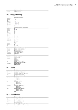
![MATLAB commands in numerical Python 24
Vidar Bronken Gundersen /mathesaurus.sf.net
Ternary operator (if?true:false)
R ifelse(a>0,a,0)
a > 0?a : 0
gnuplot a>0?a:0
idl a>0?a:0
10.3 Debugging
Most recent evaluated expression
matlab ans
R .Last.value
Axiom %
Maxima %
List variables loaded into memory
matlab whos or who
R objects()
idl help
Clear variable x from memory
matlab clear x or clear [all]
R rm(x)
Axiom )clear properties x
Print
matlab disp(a)
R print(a)
Python print a
idl print, a
10.4 Working directory and OS
List files in directory
matlab dir or ls
R list.files() or dir()
Python os.listdir(".")
idl dir
List script files in directory
matlab what
R list.files(pattern=".r$")
Python grep.grep("*.py")
Displays the current working directory
matlab pwd
R getwd()
Python os.getcwd()
gnuplot pwd
idl sd
Change working directory
matlab cd foo
Scilab chdir(’foo’)
R setwd(’foo’)
Python os.chdir(’foo’)
gnuplot cd ’foo’
idl cd,’foo or sd,’foo
Axiom )cd "foo"
Invoke a System Command
matlab !notepad
Scilab host(’notepad’)
Octave system("notepad")
R system("notepad")
Python os.system(’notepad’)
os.popen(’notepad’)
gnuplot !notepad
idl spawn,’notepad’
This document is still draft quality. Most d plot examples are made using Matplotlib, and d plots using R or Gnuplot.
Version number and download url for software used: Python .., http://www.python.org/; NumPy .., http://numeric.scipy.org/;
Matplotlib ., http://matplotlib.sf.net/; IPython .., http://ipython.scipy.org/; R .., http://www.r-project.org/; Octave ..,
http://www.octave.org/; Scilab ., http://www.scilab.org/; Gnuplot ., http://www.gnuplot.info/; Maxima .., http://maxima.sf.net/.
For referencing: Gundersen, Vidar Bronken. MATLAB commands in numerical Python (Oslo/Norway, ), available from:
http://mathesaurus.sf.net/
Contributions are appreciated: The best way to do this is to edit the xml and submit patches to our tracker or forums.](https://image.slidesharecdn.com/math-synonyms-120226112112-phpapp01/85/Math-synonyms-24-320.jpg)

This document provides a summary of commands for common mathematical operations and functions in MATLAB and their equivalents in other numerical computing environments like Python, R, Octave, and GNUPLOT. It covers topics like getting help, searching documentation, arithmetic and relational operators, and starting/ending an interactive session. The goal is to provide a quick reference for those switching between different open-source alternatives to MATLAB.