This document provides a summary of the differences between the syntax and functions of SCILAB and MATLAB. It notes that while SCILAB and MATLAB functions are often similar, there are some key differences in how functions are defined, variables are used, strings are handled, and empty matrices are operated on. It also provides a table comparing common functions between the two platforms and lists some SCILAB functions that are designed to emulate MATLAB functions. The document is intended to help users familiar with MATLAB transition to using SCILAB.

1. Comparison of SCILAB Syntax and
Functions to MATLAB®
By
Gilberto E. Urroz, Ph.D., P.E.
Distributed by
i nfoClearinghouse.com
©2001 Gilberto E. Urroz
All Rights Reserved

2. A "zip" file containing all of the programs in this document (and other
SCILAB documents at InfoClearinghouse.com) can be downloaded at the
following site:
http://www.engineering.usu.edu/cee/faculty/gurro/Software_Calculators/Scil
ab_Docs/ScilabBookFunctions.zip
The author's SCILAB web page can be accessed at:
http://www.engineering.usu.edu/cee/faculty/gurro/Scilab.html
Please report any errors in this document to: gurro@cc.usu.edu

3. COMPARING SCILAB AND MATLAB® 2
Functions 2
Comment lines 2
Variables 2
Strings 2
Boolean variables 2
Polynomials 3
Empty matrices 3
Plotting 3
Scicos 3
A table of Matlab® and SCILAB equivalent functions 3
SCILAB functions that emulate Matlab® functions 4
Graphics functions with mtlb_ prefix 5
Function mtlb_mesh 7
Download at InfoClearinghouse.com 1 © 2001 Gilberto E. Urroz

4. Comparing SCILAB and Matlab®
If the reader has previously used Matlab®, he or she would notice that the operation and, in
many instances, the syntax, of SCILAB commands are very similar to those of Matlab®. Some of
the information presented in this chapter is taken from the SCILAB web page:
http://www-rocq.inria.fr/scilab/
It is intended as a guideline highlighting the differences between SCILAB and Matlab®. The
differences are presented according to the subjects of functions, comment lines, strings,
Boolean variables, polynomials, operations on empty matrices, plotting, and SCICOS (SCILAB’s
system simulation software).
Functions
Functions in SCILAB are not considered as separate files, such as Matlab® m-files, but as
variables in the SCILAB environment. One or several user-defined functions can be defined in
a single file, and the name of the file is not necessarily related to the name of the function(s).
Also, the function(s) are not automatically loaded into SCILAB, as they are in Matlab® after
their name is invoked. Usually you have to execute the command getf(“function_name”)
before being able to use a function.
Functions can also be defined on-line (referred to as inside functions) by using the command
deff. Many examples of the use of getf and deff are provided throughout the book.
To execute a script file you must use exec("filename") in SCILAB, as in Matlab®, you just
need to type the name of the file.
Comment lines
SCILAB comments begins with: //
Matlab® comments begins with: %
Variables
Predefined variables usually have the % prefix in SCILAB (%i, %inf, ...). They are write
protected, i.e., they can not be redefined. Matlab® predefines variables i and j as the unit
imaginary number. This predefinitions can wreck havoc in programming if you try to use i or j
as index variables. Such a problem does not exist in SCILAB.
Strings
Strings are considered as 1 by 1 matrices of strings in SCILAB. Each entry of a string matrix has
its own length.
Boolean variables
Boolean variables are %T, %F in SCILAB and 0, 1 in Matlab®. They correspond to the Boolean
statements ‘true’ and ‘false’, respectively. Indexing with Boolean variables may not produce
the same result in SCILAB as it does in Matlab® . For example x=[1,2];x([1,1]) [which is NOT
x([%T,%T])] returns [1,1] in SCILAB and [1,2] in Matlab®. Also if x is a matrix x(1:n,1)=[]
or x(:)=[] are not valid in Matlab®.
Download at InfoClearinghouse.com 2 © 2001 Gilberto E. Urroz

5. Polynomials
Polynomials and polynomial matrices are defined by the function poly in SCILAB. They are
considered as vectors of coefficients in Matlab®. For more details on SCILAB polynomials see
Chapter 8 in this book.
Empty matrices
[]+1 returns 1 in SCILAB and [] in Matlab®.
Plotting
Except for the simple plot and mesh (Matlab®) and plot3d(SCILAB) functions, SCILAB and
Matlab® graph functions are not compatible. In a subsequent section we introduce some
SCILAB functions written specifically to emulate Matlab® function.
Scicos
SCICOS (SCILAB) and Simulink (Matlab®) are not compatible. SCICOS and Simulink are
graphically-based, system modeling software programs. To obtain more information about
SCICOS, visit SCILAB’s main web page (http://www-rocq.inria.fr/scilab/).
A table of Matlab® and SCILAB equivalent functions
Most built in functions are identical in Matlab® and SCILAB. Some of them have a slightly
different syntax. Here is a brief, partial list of commands with significantly different syntax.
__________________________________________
Matlab® SCILAB .
all and
any or
balance balanc
clock unix('date')
computer unix_g('machine')
cputime timer
delete unix('rm file')
dir unix_g('ls')
echo mode
eig spec or bdiag
eval evstr
exist exists + type
fclose file('close')
feof
ferror
feval evstr and strcat
filter rtitr
finite (x < %inf)
fopen file('open')
fread read
fseek file
Download at InfoClearinghouse.com 3 © 2001 Gilberto E. Urroz

6. ftell
fwrite writeb
global
home
isglobal
isinf(a) a == %inf
isnan(a) a ~= a
isstr(a) type(a) == 10
keyboard pause + resume
lasterr
lookfor apropos
more lines
pack stacksize
pause halt
qz gspec+gschur
randn rand
rem modulo
setstr code2str
strcmp(a,b) a == b
uicontrol
uimenu getvalue
unix unix_g
version
which whereis
nargin [nargout,nargin]=argn(0)
nargout
__________________________________________________
SCILAB functions that emulate Matlab® functions
For those who have used Matlab®, and for those who want to learn how to use them, SCILAB
provides a number of functions that emulate Matlab® functions. These functions start with the
prefix mtlb_. A list of the Matlab® emulating functions follows:
mtlb mtlb_all mtlb_any mtlb_axes
mtlb_cell mtlb_choices mtlb_clf mtlb_cumsum
mtlb_diff mtlb_e mtlb_eval mtlb_exist
mtlb_eye mtlb_fft mtlb_filter mtlb_find
mtlb_findstr mtlb_fliplr mtlb_flipud mtlb_fprintf
mtlb_fread mtlb_fscanf mtlb_fwrite mtlb_get
mtlb_hold mtlb_i mtlb_ifft mtlb_is
mtlb_ishold mtlb_isreal mtlb_length mtlb_load
mtlb_loglog mtlb_max mtlb_mean mtlb_median
mtlb_mesh mtlb_meshdom mtlb_min mtlb_ones
mtlb_plot mtlb_prod mtlb_qz mtlb_rand
mtlb_save mtlb_semilogx mtlb_semilogy mtlb_sprintf
mtlb_sscanf mtlb_subplot mtlb_sum mtlb_zeros
Out of these functions we have used mtlb_diff to produce table of differences in the
polynomial approximations of Chapter 8 and for the first differences in time series of Chapter
18, and mtlb_subplot in function multiplot presented in Chapter 17 in relation to multiple
linear regression.
Download at InfoClearinghouse.com 4 © 2001 Gilberto E. Urroz

7. Graphics functions with mtlb_ prefix
Help for these functions is not available in SCILAB. My take on this is that SCILAB developers
try to encourage the use of the equivalent SCILAB functions. However, some mtlb_ functions,
particular those related to handling of graphs, may be easier to use than their SCILAB
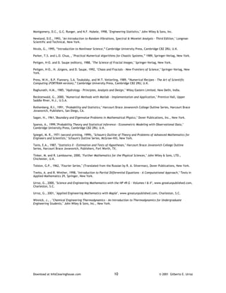
counterparts. As an example, take functions mtlb_loglog, mtlb_semilogx, mtlb_semilogy, and
mtlb_subplot. Functions mtlb_semilogx and mtlb_semilogy are intended to produce plots
with logarithmic scales in x and y, respectively, while function loglog produces plots with two
logarithmic scales. Examples of using mtlb_loglog, mtlb_semilogx, and mtlb_semilogy, are
shown below. Function mtlb_subplot will be illustrated later.
-->x=[0.001 0.01 0.1 1.0 10. 100]; y=[20 30 40 50 60 70];
-->mtlb_semilogx(x,y)
-->xtitle('Logarithmic scale in the x axis','x','y')
-->x=[1:0.1:10];y=2*x^2;
-->mtlb_semilogy(x,y)
-->xtitle('Logarithmic scale in y','x','y')
Download at InfoClearinghouse.com 5 © 2001 Gilberto E. Urroz

8. -->x=[0.001,0.01,0.1,1.0,10.0,100.0];y=x^3;
-->mtlb_loglog(x,y)
-->xtitle('Log-log plot','x','y')
The function mtlb_subplot can be used to produce multiple plot frames in the same window.
The call to mtlb_subplot is
mtlb_subplot(m,n,j)
The effect of this function is to split the plot area in a window into a graphics matrix of m rows
and n columns, making the sub-area j available for plotting. The values of j range from 1 to p
= m⋅n, with subplot j=1 corresponding to the upper left corner of the window, subplot j=2 being
the next subplot to the right, j=3 the next subplot to the right until reaching j=m. Subplot
j=m+1 is the first subplot in the second line, and so on. The position and numbering of the
subplots is shown in the next sketch.
Download at InfoClearinghouse.com 6 © 2001 Gilberto E. Urroz

9. Thus, the plot at location (i,k) is subplot number j = (i-1)m+k. To fill the window with plots
you need to call function mtlb_subplot a total of p times using fixed values of m and n and
varying j according to the position of the plot.
An example of application of function mtlb_subplot is provided next in the form of a SCILAB
script:
//Script to produce four plots in the same window
x=[0.0:0.1:1.0];y=x^2;z=sin(x)+sin(2*x);t=(1./(1+x))';r=abs(x-0.5);
mtlb_subplot(2,2,1);plot2d(x,y,-2);xtitle('Plot 1','x','y');
mtlb_subplot(2,2,2);plot2d(x,z,-1);xtitle('Plot 2','x','z');
mtlb_subplot(2,2,3);plot2d(x,t,-9);xtitle('Plot 3','x','t');
mtlb_subplot(2,2,4);plot2d(x,r,-5);xtitle('Plot 4','x','r');
The result of the script is shown next:
Function mtlb_mesh
Function mtlb_mesh can be used to produce a three-dimensional surface plot that emphasizes
the coordinate mesh in the final plot. The function produces a plot similar to that produced
with function plot3d.
-->deff(‘[w]=f(x,y)’,’w=sin(x)*cos(y)’)
--> x=[0:0.2:6];y=[0:0.2:6]; z = feval(x,y,f);
-->mtlb_mesh(x,y,z);
Download at InfoClearinghouse.com 7 © 2001 Gilberto E. Urroz

10. Note: Function mtlb_e does not have a Matlab® equivalent (at least not with the name e).
The function is intended to extract characters out of a string, for example:
--> a = ‘tres tristes tigres’
--> mtlb_e(a,[1:3])
ans = t
Download at InfoClearinghouse.com 8 © 2001 Gilberto E. Urroz

11. REFERENCES (for all SCILAB documents at InfoClearinghouse.com)
Abramowitz, M. and I.A. Stegun (editors), 1965,"Handbook of Mathematical Functions with Formulas, Graphs, and
Mathematical Tables," Dover Publications, Inc., New York.
Arora, J.S., 1985, "Introduction to Optimum Design," Class notes, The University of Iowa, Iowa City, Iowa.
Asian Institute of Technology, 1969, "Hydraulic Laboratory Manual," AIT - Bangkok, Thailand.
Berge, P., Y. Pomeau, and C. Vidal, 1984,"Order within chaos - Towards a deterministic approach to turbulence," John
Wiley & Sons, New York.
Bras, R.L. and I. Rodriguez-Iturbe, 1985,"Random Functions and Hydrology," Addison-Wesley Publishing Company,
Reading, Massachussetts.
Brogan, W.L., 1974,"Modern Control Theory," QPI series, Quantum Publisher Incorporated, New York.
Browne, M., 1999, "Schaum's Outline of Theory and Problems of Physics for Engineering and Science," Schaum's
outlines, McGraw-Hill, New York.
Farlow, Stanley J., 1982, "Partial Differential Equations for Scientists and Engineers," Dover Publications Inc., New
York.
Friedman, B., 1956 (reissued 1990), "Principles and Techniques of Applied Mathematics," Dover Publications Inc., New
York.
Gomez, C. (editor), 1999, “Engineering and Scientific Computing with Scilab,” Birkhäuser, Boston.
Gullberg, J., 1997, "Mathematics - From the Birth of Numbers," W. W. Norton & Company, New York.
Harman, T.L., J. Dabney, and N. Richert, 2000, "Advanced Engineering Mathematics with MATLAB® - Second edition,"
Brooks/Cole - Thompson Learning, Australia.
Harris, J.W., and H. Stocker, 1998, "Handbook of Mathematics and Computational Science," Springer, New York.
Hsu, H.P., 1984, "Applied Fourier Analysis," Harcourt Brace Jovanovich College Outline Series, Harcourt Brace
Jovanovich, Publishers, San Diego.
Journel, A.G., 1989, "Fundamentals of Geostatistics in Five Lessons," Short Course Presented at the 28th International
Geological Congress, Washington, D.C., American Geophysical Union, Washington, D.C.
Julien, P.Y., 1998,”Erosion and Sedimentation,” Cambridge University Press, Cambridge CB2 2RU, U.K.
Keener, J.P., 1988, "Principles of Applied Mathematics - Transformation and Approximation," Addison-Wesley
Publishing Company, Redwood City, California.
Kitanidis, P.K., 1997,”Introduction to Geostatistics - Applications in Hydogeology,” Cambridge University Press,
Cambridge CB2 2RU, U.K.
Koch, G.S., Jr., and R. F. Link, 1971, "Statistical Analysis of Geological Data - Volumes I and II," Dover Publications,
Inc., New York.
Korn, G.A. and T.M. Korn, 1968, "Mathematical Handbook for Scientists and Engineers," Dover Publications, Inc., New
York.
Kottegoda, N. T., and R. Rosso, 1997, "Probability, Statistics, and Reliability for Civil and Environmental Engineers,"
The Mc-Graw Hill Companies, Inc., New York.
Kreysig, E., 1983, "Advanced Engineering Mathematics - Fifth Edition," John Wiley & Sons, New York.
Lindfield, G. and J. Penny, 2000, "Numerical Methods Using Matlab®," Prentice Hall, Upper Saddle River, New Jersey.
Magrab, E.B., S. Azarm, B. Balachandran, J. Duncan, K. Herold, and G. Walsh, 2000, "An Engineer's Guide to
MATLAB®", Prentice Hall, Upper Saddle River, N.J., U.S.A.
McCuen, R.H., 1989,”Hydrologic Analysis and Design - second edition,” Prentice Hall, Upper Saddle River, New Jersey.
Middleton, G.V., 2000, "Data Analysis in the Earth Sciences Using Matlab®," Prentice Hall, Upper Saddle River, New
Jersey.
Download at InfoClearinghouse.com 9 © 2001 Gilberto E. Urroz

12. Montgomery, D.C., G.C. Runger, and N.F. Hubele, 1998, "Engineering Statistics," John Wiley & Sons, Inc.
Newland, D.E., 1993, "An Introduction to Random Vibrations, Spectral & Wavelet Analysis - Third Edition," Longman
Scientific and Technical, New York.
Nicols, G., 1995, “Introduction to Nonlinear Science,” Cambridge University Press, Cambridge CB2 2RU, U.K.
Parker, T.S. and L.O. Chua, , "Practical Numerical Algorithms for Chaotic Systems,” 1989, Springer-Verlag, New York.
Peitgen, H-O. and D. Saupe (editors), 1988, "The Science of Fractal Images," Springer-Verlag, New York.
Peitgen, H-O., H. Jürgens, and D. Saupe, 1992, "Chaos and Fractals - New Frontiers of Science," Springer-Verlag, New
York.
Press, W.H., B.P. Flannery, S.A. Teukolsky, and W.T. Vetterling, 1989, “Numerical Recipes - The Art of Scientific
Computing (FORTRAN version),” Cambridge University Press, Cambridge CB2 2RU, U.K.
Raghunath, H.M., 1985, "Hydrology - Principles, Analysis and Design," Wiley Eastern Limited, New Delhi, India.
Recktenwald, G., 2000, "Numerical Methods with Matlab - Implementation and Application," Prentice Hall, Upper
Saddle River, N.J., U.S.A.
Rothenberg, R.I., 1991, "Probability and Statistics," Harcourt Brace Jovanovich College Outline Series, Harcourt Brace
Jovanovich, Publishers, San Diego, CA.
Sagan, H., 1961,"Boundary and Eigenvalue Problems in Mathematical Physics," Dover Publications, Inc., New York.
Spanos, A., 1999,"Probability Theory and Statistical Inference - Econometric Modeling with Observational Data,"
Cambridge University Press, Cambridge CB2 2RU, U.K.
Spiegel, M. R., 1971 (second printing, 1999), "Schaum's Outline of Theory and Problems of Advanced Mathematics for
Engineers and Scientists," Schaum's Outline Series, McGraw-Hill, New York.
Tanis, E.A., 1987, "Statistics II - Estimation and Tests of Hypotheses," Harcourt Brace Jovanovich College Outline
Series, Harcourt Brace Jovanovich, Publishers, Fort Worth, TX.
Tinker, M. and R. Lambourne, 2000, "Further Mathematics for the Physical Sciences," John Wiley & Sons, LTD.,
Chichester, U.K.
Tolstov, G.P., 1962, "Fourier Series," (Translated from the Russian by R. A. Silverman), Dover Publications, New York.
Tveito, A. and R. Winther, 1998, "Introduction to Partial Differential Equations - A Computational Approach," Texts in
Applied Mathematics 29, Springer, New York.
Urroz, G., 2000, "Science and Engineering Mathematics with the HP 49 G - Volumes I & II", www.greatunpublished.com,
Charleston, S.C.
Urroz, G., 2001, "Applied Engineering Mathematics with Maple", www.greatunpublished.com, Charleston, S.C.
Winnick, J., , "Chemical Engineering Thermodynamics - An Introduction to Thermodynamics for Undergraduate
Engineering Students," John Wiley & Sons, Inc., New York.
Download at InfoClearinghouse.com 10 © 2001 Gilberto E. Urroz