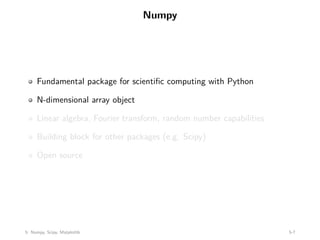
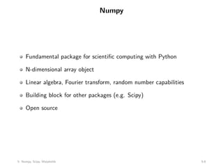
This document summarizes a lecture on Numpy, Scipy, and Matplotlib. It introduces Numpy as the fundamental package for scientific computing with Python, providing N-dimensional arrays and capabilities for linear algebra, Fourier transforms, and random numbers. Scipy is introduced as a library of algorithms and tools built to work with Numpy arrays, covering areas like linear algebra, statistics, optimization, and signal processing. Matplotlib is covered as a plotting library for Python that works well with Numpy and has a syntax similar to Matlab. Examples are provided on key capabilities and functions within each package.

![import numpy as np
Basics:
import numpy as np
A = np.array([[1, 2, 3], [4, 5, 6]])
print A
# [[1 2 3]
# [4 5 6]]
Af = np.array([1, 2, 3], float)
Slicing as usual.
5: Numpy, Scipy, Matplotlib 5-9](https://image.slidesharecdn.com/lec5-240215144438-0b60731d/85/Lecture-5-of-Stanford-university-about-python-librarys-9-320.jpg)
![More basics
np.arange(0, 1, 0.2)
# array([ 0. , 0.2, 0.4, 0.6, 0.8])
np.linspace(0, 2*np.pi, 4)
# array([ 0.0, 2.09, 4.18, 6.28])
A = np.zeros((2,3))
# array([[ 0., 0., 0.],
# [ 0., 0., 0.]])
# np.ones, np.diag
A.shape
# (2, 3)
5: Numpy, Scipy, Matplotlib 5-10](https://image.slidesharecdn.com/lec5-240215144438-0b60731d/85/Lecture-5-of-Stanford-university-about-python-librarys-10-320.jpg)
![More basics
np.random.random((2,3))
# array([[ 0.78084261, 0.64328818, 0.55380341],
# [ 0.24611092, 0.37011213, 0.83313416]])
a = np.random.normal(loc=1.0, scale=2.0, size=(2,2))
# array([[ 2.87799514, 0.6284259 ],
# [ 3.10683164, 2.05324587]])
np.savetxt("a_out.txt", a)
# save to file
b = np.loadtxt("a_out.txt")
# read from file
5: Numpy, Scipy, Matplotlib 5-11](https://image.slidesharecdn.com/lec5-240215144438-0b60731d/85/Lecture-5-of-Stanford-university-about-python-librarys-11-320.jpg)
![Arrays are mutable
A = np.zeros((2, 2))
# array([[ 0., 0.],
# [ 0., 0.]])
C = A
C[0, 0] = 1
print A
# [[ 1. 0.]
# [ 0. 0.]]
5: Numpy, Scipy, Matplotlib 5-12](https://image.slidesharecdn.com/lec5-240215144438-0b60731d/85/Lecture-5-of-Stanford-university-about-python-librarys-12-320.jpg)
![Basic operations
Arithmetic operators: elementwise application
a = np.arange(4)
# array([0, 1, 2, 3])
b = np.array([2, 3, 2, 4])
a * b # array([ 0, 3, 4, 12])
b - a # array([2, 2, 0, 1])
c = [2, 3, 4, 5]
a * c # array([ 0, 3, 8, 15])
Also, we can use += and *=.
5: Numpy, Scipy, Matplotlib 5-14](https://image.slidesharecdn.com/lec5-240215144438-0b60731d/85/Lecture-5-of-Stanford-university-about-python-librarys-14-320.jpg)
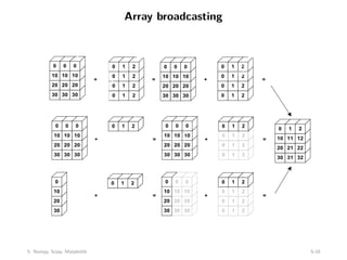
![Array broadcasting with scalars
This also allows us to add a constant to a matrix or multiply a matrix by
a constant
A = np.ones((3,3))
print 3 * A - 1
# [[ 2. 2. 2.]
# [ 2. 2. 2.]
# [ 2. 2. 2.]]
5: Numpy, Scipy, Matplotlib 5-17](https://image.slidesharecdn.com/lec5-240215144438-0b60731d/85/Lecture-5-of-Stanford-university-about-python-librarys-17-320.jpg)
![Vector operations
inner product
outer product
dot product (matrix multiplication)
# note: numpy automatically converts lists
u = [1, 2, 3]
v = [1, 1, 1]
np.inner(u, v)
# 6
np.outer(u, v)
# array([[1, 1, 1],
# [2, 2, 2],
# [3, 3, 3]])
np.dot(u, v)
# 6
5: Numpy, Scipy, Matplotlib 5-18](https://image.slidesharecdn.com/lec5-240215144438-0b60731d/85/Lecture-5-of-Stanford-university-about-python-librarys-18-320.jpg)
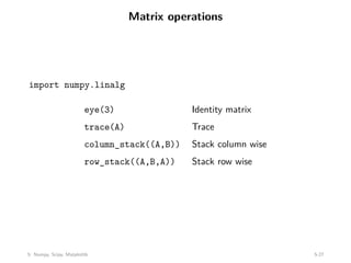
![Matrix operations
First, define some matrices:
A = np.ones((3, 2))
# array([[ 1., 1.],
# [ 1., 1.],
# [ 1., 1.]])
A.T
# array([[ 1., 1., 1.],
# [ 1., 1., 1.]])
B = np.ones((2, 3))
# array([[ 1., 1., 1.],
# [ 1., 1., 1.]])
5: Numpy, Scipy, Matplotlib 5-19](https://image.slidesharecdn.com/lec5-240215144438-0b60731d/85/Lecture-5-of-Stanford-university-about-python-librarys-19-320.jpg)
![Matrix operations
np.dot(A, B)
# array([[ 2., 2., 2.],
# [ 2., 2., 2.],
# [ 2., 2., 2.]])
np.dot(B, A)
# array([[ 3., 3.],
# [ 3., 3.]])
np.dot(B.T, A.T)
# array([[ 2., 2., 2.],
# [ 2., 2., 2.],
# [ 2., 2., 2.]])
np.dot(A, B.T)
# Traceback (most recent call last):
# File "<stdin>", line 1, in <module>
# ValueError: shapes (3,2) and (3,2) not aligned: ...
# ... 2 (dim 1) != 3 (dim 0)
5: Numpy, Scipy, Matplotlib 5-20](https://image.slidesharecdn.com/lec5-240215144438-0b60731d/85/Lecture-5-of-Stanford-university-about-python-librarys-20-320.jpg)
![Operations along axes
a = np.random.random((2,3))
# array([[ 0.9190687 , 0.36497813, 0.75644216],
# [ 0.91938241, 0.08599547, 0.49544003]])
a.sum()
# 3.5413068994445549
a.sum(axis=0) # column sum
# array([ 1.83845111, 0.4509736 , 1.25188219])
a.cumsum()
# array([ 0.9190687 , 1.28404683, 2.04048899, 2.9598714 ,
# 3.04586687, 3.5413069 ])
a.cumsum(axis=1) # cumulative row sum
# array([[ 0.9190687 , 1.28404683, 2.04048899],
# [ 0.91938241, 1.00537788, 1.50081791]])
a.min()
# 0.0859954690403677
a.max(axis=0)
# array([ 0.91938241, 0.36497813, 0.75644216])
5: Numpy, Scipy, Matplotlib 5-21](https://image.slidesharecdn.com/lec5-240215144438-0b60731d/85/Lecture-5-of-Stanford-university-about-python-librarys-21-320.jpg)
![Slicing arrays
More advanced slicing
a = np.random.random((4,5))
a[2, :]
# third row, all columns
a[1:3]
# 2nd, 3rd row, all columns
a[:, 2:4]
# all rows, columns 3 and 4
5: Numpy, Scipy, Matplotlib 5-22](https://image.slidesharecdn.com/lec5-240215144438-0b60731d/85/Lecture-5-of-Stanford-university-about-python-librarys-22-320.jpg)
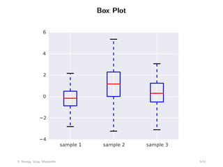
![Box Plot
samp1 = np.random.normal(loc=0., scale=1., size=100)
samp2 = np.random.normal(loc=1., scale=2., size=100)
samp3 = np.random.normal(loc=0.3, scale=1.2, size=100)
f, ax = plt.subplots(1, 1, figsize=(5,4))
ax.boxplot((samp1, samp2, samp3))
ax.set_xticklabels([’sample 1’, ’sample 2’, ’sample 3’])
plt.savefig(’boxplot.pdf’)
5: Numpy, Scipy, Matplotlib 5-50](https://image.slidesharecdn.com/lec5-240215144438-0b60731d/85/Lecture-5-of-Stanford-university-about-python-librarys-50-320.jpg)