This document provides notes for a multivariable calculus class covering vector-valued functions. It begins with an introduction to vector-valued functions, defining them as functions whose domain is real numbers and range is vectors. It discusses limits of vector functions and continuity. It then covers derivatives and integrals of vector functions, defining the derivative similarly to real-valued functions. It provides theorems on computing derivatives of vector functions by taking derivatives of the component functions. The document concludes with discussing tangent vectors and lines for vector functions.
In this presentation, a more accurate expression of the zeta zero-counting function is developed exhibiting the expected step function behavior and its relation to the primes is demonstrated.
In this presentation, a more accurate expression of the zeta zero-counting function is developed exhibiting the expected step function behavior and its relation to the primes is demonstrated.
A set of notes prepared for an introductory machine learning course, assuming very limited linear algebra background, because all linear algebra operations are fully written out. These notes go into thorough derivations of the generalized linear regression formulation, demonstrating how to write it out in matrix form.
On The Function D(s) Associated With Riemann Zeta Functioninventionjournals
We consider the function D(s) of the complex argument s=+it, formed with the use of a certain procedure of a transition to the limit. For >1 the function D reduces to the Riemann zeta function, multiplied by the factor (s-1). For <1>1 is presented. "Zeta effect" was discovered-the formation of fictitious short-period oscillations D(s), caused by the confinement of a finite number of terms in the summation of Riemann series containing a large number of harmonics with a slowly varying frequency. A procedure for the numerical suppression of these zeta oscillations is proposed. On the line =1, where D(s) is undefined, an infinite family of "Riemann functions", genetically related to the Riemann zeta function, is introduced. A numerical investigation of these "Riemannian curves" is presented.
I am Bing Jr. I am a Signal Processing Assignment Expert at matlabassignmentexperts.com. I hold a Master's in Matlab Deakin University, Australia. I have been helping students with their assignments for the past 9 years. I solve assignments related to Signal Processing.
Visit matlabassignmentexperts.com or email info@matlabassignmentexperts.com. You can also call on +1 678 648 4277 for any assistance with Signal Processing Assignments.
The paper reports on an iteration algorithm to compute asymptotic solutions at any order for a wide class of nonlinear
singularly perturbed difference equations.
Explicit Formula for Riemann Prime Counting FunctionKannan Nambiar
Corresponding to every zeta function there is a delta series. We make use of this fact to derive an explicit formula for Riemann Prime Counting Function.
MGMT 511Location ProblemGeorge Heller was so successful in.docxandreecapon
MGMT 511
Location Problem
George Heller was so successful in his previous assignment that he was promoted to the coveted position of Infrastructure Manager on the Mergers and Acquisitions Team.
Again Agame has recently acquired a competitive company with a plant and a warehouse in a nearby city. Management has decided to keep the additional warehouse. However, they are unsure if they need to keep the additional manufacturing plant. All products can be manufactured in either plant and shipped from either warehouse. Each plant and each warehouse has sufficient capacity to meet the total forecasted demand individually.
Prepare a report for management with your recommendation. Three possible choices exist. 1) Close the Competitor plant and satisfy all demand from the Again Agame plant; 2) Close the Again Agame plant and satisfy all demand from the Competitor plant; 3)Keep both plants open.
Your recommendation should include a solution for each of the five years in question. Include your calculations and spreadsheets in support of your recommendations.
Sales Forecast (cases)
2011
2012
2013
2014
2015
Competitor Warehouse (WH1)
15,000,000
20,000,000
26,000,000
34,000,000
44,000,000
Again Agame Warehouse (WH2)
6,000,000
7,000,000
10,000,000
15,000,000
21,000,000
Fixed Costs
2011
2012
2013
2014
2015
Competitor Plant (P1)
900,000
900,000
900,000
900,000
900,000
Again Agame Plant (P2)
800,000
800,000
800,000
800,000
800,000
Transportation Costs
$1.00 / 1,000 cases / mile
4
Costs -- Both Plant Scenario
20112012201320142015
Transport P1 - WH1
Transport P2 - WH2
Fixed Cost - P1
Fixed Cost - P2
Total
General Info.Infrastructure ExerciseDate: 28/10/97Situation:a) Package -RGBb) Nr. Plants -2c) Nr. WH -2d) Period -5 yearse) Sales Frcst. -DecreasingCapacity MM U/C per Year:Plant 1 -5avg. HK 70 (KS)Plant 2 -3avg. HK 42 (KS)Distance Matrix: (Km)WH1WH2P150600P2600100Diagram:
&A
Page &P
WH2
Franchise 2
Franchise 1
P2
P1
WH1
Sales Frcst.Infrastructure ExerciseDate: 28/10/97Sales Forecast (M U.C)RGB'98'99'00'01'02WH15000.04000.03400.02800.02400.0WH23000.02400.02000.01600.01400.0Obs. Volume is Decreasing 15% per year.
&A
Page &P
CostsInfrastructure ExerciseDate: 28/10/97Transport Costs:0.51,000 cases per KmFixed Costs:900,000P1 = $600,000/year800,000P2 = $500,000/year
&A
Page &P
AnalysisInfrastructure ExerciseDate: 28/10/97Fixed Costs'98'99'00'01'02P1800,000800,000800,000800,000800,000P2700,000700,000700,000700,000700,000Total1,500,0001,500,0001,500,0001,500,0001,500,000Transportation Costs'98'99'00'01'02P1 - WH1125,000100,00085,00070,00060,000P2 - WH2150,000120,000100,00080,00070,000P1 - WH2900,000720,000600,000480,000420,000P2 - WH11,500,0001,200,0001,020,000840,000720,000Total 1275,000220,000185,000150,000130,000(both plants)Total 21,025,000820,000685 ...
MGMT 464From Snowboarders to Lawnmowers Case Study Case An.docxandreecapon
MGMT 464
From Snowboarders to Lawnmowers Case Study
Case Analysis Worksheet #1
Case Analysis Session 1 : Focus on Inspiring a Shared Vision (Principle #2)
Inspiring a shared vision has two main components [1] creating a vision through common purpose, and [2] enlisting or getting people ‘on board’ with the vision.
In your small groups, discuss and document your group’s response to the following questions. Upload your typed document into one of your group member’s D2L dropbox by the assigned due date on your course schedule. Be sure to include on your worksheet all group member names. If present in class, all group members will receive the same grade for this case analysis assignment (maximum 30 pts). Group peer evaluations will be used to determine overall individual group member participation points for both of these case study discussions (maximum 15 pts).
1. In what specific ways did Michael fail and/or succeed in ‘listening deeply’ to his employees?
2. In what specific ways did Michael show that he was not “open to influence?” How would Michael being open to influence have made him more effective, ( i.e., who were the “local experts” and how could he have benefited from them)?
3. When you consider the employees of Bedford Mower as they were before Michael arrived, how would you characterize them in terms of what was personally meaningful to them?
4. When creating his vision for the company, in what specific ways did Michael fail and/or succeed in ‘determining what was meaningful’ to his employees, and what was the impact?
5. What specific mechanisms, or opportunities did Michael have available to him for enlisting others?
6. To what extent did Michael take advantage of these? To what extent were they effective in terms of getting everyone on board with the new vision?
7. In thinking about his attempts to enlist others, in what ways did or didn’t Michael incorporate common ideals into his communication with his employees as it related to the new vision?
8. How successful was Michael in “animating the vision”? How would you characterize him in terms of his use of symbolic language, providing imagery of the future, practicing positive communication, expressing emotion, and speaking from the heart, in his communications to his employees?
9. What would you have done differently with this group of employees in terms of inspiring a shared vision?
Team Leadership Case
From Snowboards to Lawnmowers
Michael Francis, a man in his late 30s, born and raised in Oregon, was an avid snowboarder. He was known among his many friends and associates as a risk-taker, highly intelligent, innovative, a bit of a rebel, but an extremely smart businessman. When he was in his early 20s, he started his own snowboarding company designing and manufacturing what became known as some of the most cutting edge boards available. Having recently married a woman who was raised on the East coast, he decided to sell his company and move to Vermont where h ...
More Related Content
Similar to MATH 200-004 Multivariate Calculus Winter 2014Chapter 12.docx
A set of notes prepared for an introductory machine learning course, assuming very limited linear algebra background, because all linear algebra operations are fully written out. These notes go into thorough derivations of the generalized linear regression formulation, demonstrating how to write it out in matrix form.
On The Function D(s) Associated With Riemann Zeta Functioninventionjournals
We consider the function D(s) of the complex argument s=+it, formed with the use of a certain procedure of a transition to the limit. For >1 the function D reduces to the Riemann zeta function, multiplied by the factor (s-1). For <1>1 is presented. "Zeta effect" was discovered-the formation of fictitious short-period oscillations D(s), caused by the confinement of a finite number of terms in the summation of Riemann series containing a large number of harmonics with a slowly varying frequency. A procedure for the numerical suppression of these zeta oscillations is proposed. On the line =1, where D(s) is undefined, an infinite family of "Riemann functions", genetically related to the Riemann zeta function, is introduced. A numerical investigation of these "Riemannian curves" is presented.
I am Bing Jr. I am a Signal Processing Assignment Expert at matlabassignmentexperts.com. I hold a Master's in Matlab Deakin University, Australia. I have been helping students with their assignments for the past 9 years. I solve assignments related to Signal Processing.
Visit matlabassignmentexperts.com or email info@matlabassignmentexperts.com. You can also call on +1 678 648 4277 for any assistance with Signal Processing Assignments.
The paper reports on an iteration algorithm to compute asymptotic solutions at any order for a wide class of nonlinear
singularly perturbed difference equations.
Explicit Formula for Riemann Prime Counting FunctionKannan Nambiar
Corresponding to every zeta function there is a delta series. We make use of this fact to derive an explicit formula for Riemann Prime Counting Function.
MGMT 511Location ProblemGeorge Heller was so successful in.docxandreecapon
MGMT 511
Location Problem
George Heller was so successful in his previous assignment that he was promoted to the coveted position of Infrastructure Manager on the Mergers and Acquisitions Team.
Again Agame has recently acquired a competitive company with a plant and a warehouse in a nearby city. Management has decided to keep the additional warehouse. However, they are unsure if they need to keep the additional manufacturing plant. All products can be manufactured in either plant and shipped from either warehouse. Each plant and each warehouse has sufficient capacity to meet the total forecasted demand individually.
Prepare a report for management with your recommendation. Three possible choices exist. 1) Close the Competitor plant and satisfy all demand from the Again Agame plant; 2) Close the Again Agame plant and satisfy all demand from the Competitor plant; 3)Keep both plants open.
Your recommendation should include a solution for each of the five years in question. Include your calculations and spreadsheets in support of your recommendations.
Sales Forecast (cases)
2011
2012
2013
2014
2015
Competitor Warehouse (WH1)
15,000,000
20,000,000
26,000,000
34,000,000
44,000,000
Again Agame Warehouse (WH2)
6,000,000
7,000,000
10,000,000
15,000,000
21,000,000
Fixed Costs
2011
2012
2013
2014
2015
Competitor Plant (P1)
900,000
900,000
900,000
900,000
900,000
Again Agame Plant (P2)
800,000
800,000
800,000
800,000
800,000
Transportation Costs
$1.00 / 1,000 cases / mile
4
Costs -- Both Plant Scenario
20112012201320142015
Transport P1 - WH1
Transport P2 - WH2
Fixed Cost - P1
Fixed Cost - P2
Total
General Info.Infrastructure ExerciseDate: 28/10/97Situation:a) Package -RGBb) Nr. Plants -2c) Nr. WH -2d) Period -5 yearse) Sales Frcst. -DecreasingCapacity MM U/C per Year:Plant 1 -5avg. HK 70 (KS)Plant 2 -3avg. HK 42 (KS)Distance Matrix: (Km)WH1WH2P150600P2600100Diagram:
&A
Page &P
WH2
Franchise 2
Franchise 1
P2
P1
WH1
Sales Frcst.Infrastructure ExerciseDate: 28/10/97Sales Forecast (M U.C)RGB'98'99'00'01'02WH15000.04000.03400.02800.02400.0WH23000.02400.02000.01600.01400.0Obs. Volume is Decreasing 15% per year.
&A
Page &P
CostsInfrastructure ExerciseDate: 28/10/97Transport Costs:0.51,000 cases per KmFixed Costs:900,000P1 = $600,000/year800,000P2 = $500,000/year
&A
Page &P
AnalysisInfrastructure ExerciseDate: 28/10/97Fixed Costs'98'99'00'01'02P1800,000800,000800,000800,000800,000P2700,000700,000700,000700,000700,000Total1,500,0001,500,0001,500,0001,500,0001,500,000Transportation Costs'98'99'00'01'02P1 - WH1125,000100,00085,00070,00060,000P2 - WH2150,000120,000100,00080,00070,000P1 - WH2900,000720,000600,000480,000420,000P2 - WH11,500,0001,200,0001,020,000840,000720,000Total 1275,000220,000185,000150,000130,000(both plants)Total 21,025,000820,000685 ...
MGMT 464From Snowboarders to Lawnmowers Case Study Case An.docxandreecapon
MGMT 464
From Snowboarders to Lawnmowers Case Study
Case Analysis Worksheet #1
Case Analysis Session 1 : Focus on Inspiring a Shared Vision (Principle #2)
Inspiring a shared vision has two main components [1] creating a vision through common purpose, and [2] enlisting or getting people ‘on board’ with the vision.
In your small groups, discuss and document your group’s response to the following questions. Upload your typed document into one of your group member’s D2L dropbox by the assigned due date on your course schedule. Be sure to include on your worksheet all group member names. If present in class, all group members will receive the same grade for this case analysis assignment (maximum 30 pts). Group peer evaluations will be used to determine overall individual group member participation points for both of these case study discussions (maximum 15 pts).
1. In what specific ways did Michael fail and/or succeed in ‘listening deeply’ to his employees?
2. In what specific ways did Michael show that he was not “open to influence?” How would Michael being open to influence have made him more effective, ( i.e., who were the “local experts” and how could he have benefited from them)?
3. When you consider the employees of Bedford Mower as they were before Michael arrived, how would you characterize them in terms of what was personally meaningful to them?
4. When creating his vision for the company, in what specific ways did Michael fail and/or succeed in ‘determining what was meaningful’ to his employees, and what was the impact?
5. What specific mechanisms, or opportunities did Michael have available to him for enlisting others?
6. To what extent did Michael take advantage of these? To what extent were they effective in terms of getting everyone on board with the new vision?
7. In thinking about his attempts to enlist others, in what ways did or didn’t Michael incorporate common ideals into his communication with his employees as it related to the new vision?
8. How successful was Michael in “animating the vision”? How would you characterize him in terms of his use of symbolic language, providing imagery of the future, practicing positive communication, expressing emotion, and speaking from the heart, in his communications to his employees?
9. What would you have done differently with this group of employees in terms of inspiring a shared vision?
Team Leadership Case
From Snowboards to Lawnmowers
Michael Francis, a man in his late 30s, born and raised in Oregon, was an avid snowboarder. He was known among his many friends and associates as a risk-taker, highly intelligent, innovative, a bit of a rebel, but an extremely smart businessman. When he was in his early 20s, he started his own snowboarding company designing and manufacturing what became known as some of the most cutting edge boards available. Having recently married a woman who was raised on the East coast, he decided to sell his company and move to Vermont where h ...
MG345_Lead from Middle.pptLeading from the Middle Exe.docxandreecapon
MG345_Lead from Middle.ppt
Leading from the Middle: Exerting Influence Sideways & Upward
MG345 Organizations & Environment
Tony Buono
Fall 2104
Unfreezing
Changing
Refreezing
Planned
Change
Guided
Changing
Freezing
Rebalancing/
Translating
Unfreezing/
Improvising
Directed
Change
Present
State
Desired
State
Conceptualizing Change Processes
Low
Low
High
High
Business Complexity
Socio-Technical
Uncertainty
Authority
Acceptance
Persuasive Communication
A Question of Rhythm?
Leadership Styles
TASK FOCUS
PEOPLE FOCUS
LEARNING FOCUS
ORGANIZATIONAL EMPHASIS
INDIVIDUAL EMPHASIS
Commanding (Coercive)
Pacesetter
Visionary
(Authoritative)
Affiliative
Democratic
Coaching
EQ Adaptive Ability
Across Styles
Managers as Linking Pins
Middle Management …
“… story of gradual disempowerment in which reasonably healthy, confident and competent people become transformed into anxious, tense, ineffective and self-doubting wrecks.”
Barry Oshry, “Converting Middle Powerlessness to Middle Power,” National Productivity Review
Intervening in the MiddleConceptualizing and Understanding One’s Sphere of InfluenceControllables v. UncontrollablesControlled (Contained) EmpowermentLooking for Opportunities in AmbiguityPursuing “Small Wins”
Source: A.F. Buono & A.J. Nurick, “Intervening in the Middle: Coping Strategies in Mergers and
Acquisitions,” Human Resource Planning, 1992, vol. 15, no. 2.
Lewin’s Force-Field Analysis
Status Quo
Change Drivers
Change Resisters
2-
C
H
A
N
G
I
N
G
1-UNFREEZING
3-REFREEZING
KEY:
Own versus
Induced Forces
Dealing with ResistanceApproachUseAdvantagesDisadvantagesEducation +
CommunicationLack of or inaccurate infoHelps to inform and persuadeTime consuming, especially if many people are involvedParticipation + InvolvementInitiators do not have all info; others have considerable power to resistParticipation leads to commitment; recipient info integrated into change planTime consuming; participators can design inappropriate changeFacilitation + SupportResistance due to adjustment problemsBest way to cope with adjustment issuesCan be time consuming; can still failNegotiationSomeone/group loses out and has power to resistRelatively easy was to avoid problemsCan be expensiveManipulationOther tactics don’t’ workQuick, inexpensiveShort-term utility, can lead to future problemsExplicit + Implicit CoercionSpeed; you have powerSimple, straightforwardShort-term benefits, can be risky; retribution
“Managing” Your Boss
Understand your boss
Goals & Needs Working Style
Strengths & Weaknesses
Understand yourself
Goals & Needs Working Style
Strengths & Weaknesses How you react to your boss?
What do you do to help/hurt your relat ...
MGMT 345
Phase 2 IPBusiness MemoTo:
Warehouse ManagerFrom:[Your Name]Date:February 25, 2015Re:
Effective Supply Chain Design
Enhancing Profitability and Stakeholder Value with Effective Supply Chain Design
Supply Chain Networks
Supply Chain Drivers
Supply Chains and Distribution of Assets and Resources
Supply Chain Visual
Figure 1: The Food Production Chain.(n.d.). Retrieved from http://www.cdc.gov/foodsafety/images/food_production_chain_400px.jpg
References
Do not forget to put your references in alphabetical order (vertically, NOT horizontally) by author’s last name, and use only first initials, not first name. If one of your references begins with the word "The," put the rest of the name first and insert a comma, followed by the word The (example – Associated Press, The.).
Author's Last Name, First Initial. (year). Title of article/Internet page. Retrieved from http://complete URL here Do Not end with a period (EXAMPLE OF AN INTERNET SOURCE – IF NO DATE IS GIVEN ON THE INTERNET PAGE USE: (n.d.). IN PLACE OF THE YEAR.)
Author's Last Name, First Initial. (year). Title of book. City, ST: Publisher. (EXAMPLE OF A BOOK)
Author's Last Name, First Initial. (year, Season). Title of article. Magazine Name, 12(8), 27. (EXAMPLE OF A MAGAZINE ARTICLE - Note – only capitalize the proper nouns in the title of the article; capitalize all the words in the magazine name; the 12 is where the volume number goes, the 8 is where the issue number goes, the 27 is where the page number goes.)
Berube, M. S., ed. (1989). The American heritage dictionary. New York: Dell. (EXAMPLE OF A DICTIONARY)
Bird, I. (1973). A lady's life in the Rocky Mountains (Reprint ed.). New York: Ballantine Books. (EXAMPLE OF A BOOK)
Food Production Chain, The. (n.d.). Retrieved from http://www.cdc.gov/foodsafety/images/food_production_chain_400px.jpg
Grant, A. M. & Berry, J. W. (2011). The necessity of others is the mother of invention: Intrinsic and prosocial motivations, perspective taking, and creativity. Academy of Management Journal.54 (1), 73-96. DOI: 10.5465/AMJ.2011.59215085 (EXAMPLE FROM OUR BONUS LIVE CHAT, PLEASE VIEW THE BONUS LIVE CHAT TO SEE HOW TO FORMAT A REFERENCE WHEN RESEARCHING FROM THE CTU LIBRARY, WHICH IS REQUIRED FOR THIS TASK)
Leonard, S. J., & Noel, T. J. (1990). Denver: Mining camp to metropolis. Niwot, CO: University Press of Colorado. (EXAMPLE OF A BOOK)
Morson, B., & Frazier, D. (2000, December 7). For years, brown cloud fouls Denver image [Electronic version]. Denver (Colorado) Rocky Mountain News. Retrieved October 3, 2002, from http://insidedenver.com/millennium/1207stone.shtml (EXAMPLE OF A NEWSPAPER ARTICLE FROM AN ONLINE VERSION OF THE NEWSPAPER)
National Jewish Medical & Research Center. (2001a, January 5). The 'Brown Cloud,' cold-induced asthma, winter allergies and seasonal affective disorder around the corner as winter approaches. Retrieved October 4, 2002, from http://www.njc.org/news/ winter1.html (EXAMPLE OF AN ORGANIZATION ...
MGMT 3720 – Organizational Behavior EXAM 3
(CH. 9, 10, 11, & 12)
Question 1
1.
While discussing their marketing campaign for a new product, the members of the cross-functional team responsible for Carver Inc. realized that a couple of changes relating to their prior plan would be beneficial. The offer of a franchising that had earlier been brushed off by the company head was discussed thoroughly and it was decided that it would be implemented on a trial basis initially, and on full scale if found to work well. From the information provided, it can be concluded that this cross-functional team has a high degree of ________.
Answer
reflexivity
uncertainty
diversity
conformity
demography
Question 2
1.
Max Hiller was recently hired by Sync, a consumer goods company. During his first meeting with the sales team, Max impressed upon his team that work performance is the only criterion he would use to evaluate them. To help them perform well and meet their targets, he pushed his team to work extra hours. He also gave very clear instructions to each member regarding their job responsibilities and continually verified if they were meeting their targets. Which of the following, if true, would weaken Max's approach?
Answer
Sales figures for the region that Max's team is responsible for have improved in the last quarter.
Max is leading many new employees who have joined his team directly after training.
Max's sales team is comprised of independent and experienced employees who are committed to their jobs.
Max's team functions in a sluggish manner and picks up pace only a week or so before the monthly operations cycle meetings.
Max's team does not display high levels of cohesiveness and members fail to coordinate with each other.
Question 3
1.
Which of the following statements is true regarding the effect of group cohesiveness and performance norms on group productivity?
Answer
When both cohesiveness and performance norms are high, productivity will be high.
The productivity of the group is affected by the performance norms but not by the cohesiveness of the group.
If cohesiveness is high and performance norms are low, productivity will be high.
When cohesiveness is low and performance norms are also low, productivity will be high.
If cohesiveness is low and performance norms are high, productivity will be low.
Question 4
1.
Neutralizers make it impossible for leader behavior to make any difference to follower outcomes.
Answer
True
False
Question 5
1.
Communication includes both the transfer and the understanding of meaning.
Answer
True
False
Question 6
1.
According to the path-goal theory, directive leadership is likely to be welcomed and accepted by employees with high ability or considerable experience.
Answer
True
False
Question 7
1.
Before buying her new phone, Gina listed the various requirements her new phone must meet. As a wedding planner, much of her work revolved around usin ...
Mexico, Page 1 Running Head MEXICO’S CULTURAL, ECONOMI.docxandreecapon
Mexico, Page 1
Running Head: MEXICO’S CULTURAL, ECONOMICAL, AND POLITICAL STATE
Mexico’s Cultural, Economical, and Political State
For
Firms Pursuing Business In or With Mexico
By
Kashmala Khan
For
Athena Miklos, Professor
ECN 2025-102947
Tuesdays and Thursdays, 10:00-11:20 AM
College of Southern Maryland
La Plata, Maryland
November 15, 2012
Mexico, Page 2
Summary
Before a firm does business in Mexico it is imperative to understand the achievements
and pitfalls of its cultural, economic, and political forces. Although Mexico has improved
substantially with its technological development, investment policies, foreign exchange policies,
and tariffs, it still has significant pitfalls when it comes to honoring contracts, legal framework,
and enforcing laws.
The cultural forces of Mexico are largely dependent on social structure. Mexicans respect
authority and look to those above them for guidance and decision-making. This makes it
important to know which person is in charge, and leads to an authoritarian approach to decision-
making and problem solving. Since 92.7% of the total population in Mexico speaks Spanish
only, it will be beneficial to learn Spanish or have a translator at hand at all times. Shared culture
makes it easier to market and sell goods and services.
The economic forces in Mexico offer both favorable and unfavorable qualities. Mexico is
currently the second largest export market for U.S. goods. Some of the greatest achievements of
economic forces include physical infrastructures, telecommunication systems, production
capabilities, and technology. The unfavorable qualities of the economic forces include high
employment rate and unskilled labor.
The political forces in Mexico also play a great role in opportunities and pitfalls. The
opportunities include efficient settlements to disputes and reasonable trade regulations and
standards. The pitfalls include wars and terrorism caused by the drug wars and cartels.
There are numerous opportunities for firms in the Textiles and Clothing industry of
Mexico. A firm should be knowledgeable about the cultural differences in Mexican people in
Mexico, Page 3
order to undergo business successfully. A firm should also be aware of the potential profit
Mexico has to offer, as well as the potential problems. To conclude from this research, U.S.
firms should enter the Textiles and Clothing industry in Mexico because there are a lot of
opportunities and the Mexican economy will further expand in the near future.
Mexico, Page 4
Introduction
This paper will review and relay the most recent information regarding Mexico’s cultural,
economic, and political forces. The objective of this paper is to assist firms who are interested in
entering the Textiles and Clothing industry in Mexico by portraying the opportunities, issues,
and pros and cons of doing business in Mexico. Th ...
MGM316-1401B-01Quesadra D. GoodrumClass Discussion Phase2.docxandreecapon
MGM316-1401B-01
Quesadra D. Goodrum
Class Discussion Phase2
Colorado Technical University
Professor: Edmund Winters
4/07/2014
In an ever-changing world, intercultural business communication is one of the most vital aspects of carrying out business in foreign countries. We are set up to fail if we enter into foreign business agreements blindly. In the absence of proper communication skills, cultural awareness comes into play knowing the culture in which we are dealing. All of your concepts you may have grown up with and ideas that you have formed beforehand need to be thrown away and cast to the side. Your concepts and ideas in these business meetings will only be as effective as your communication skills. If your communications skills are weak so will be your presentation of your projected business plan. If I was going to develop a training program on the same, my lesson plan would look as illustrated below:
I. Class Objectives: The goals or objectives for class include understanding how language affects intercultural business communications and learning about different cultures and how they communicate when conducting business activities.
II. Connection to Course Goals: The class’s daily objectives will connect to the overall course goals by dealing with one topic at a time.
III. Anticipatory Set: What is usually involved in intercultural business communication and how should one behave if relocated to foreign countries such as United Arab Emirates, Mexico, China and Israel?
IV. Cultural Awareness
V. High vs. Low Context Cultures
VI. Language: Verbal vs. Non-Verbal
VII. Conversational Taboos
VIII. Interaction: Ethical/Unethical awareness
IX. Conclusion: connecting the objectives
My developed training program will help my students target and grasp the importance of the concepts listed and how they connect to one another. You will need to know a number of things regarding Cultural Awareness, High vs. Low Context Cultures, and Verbal vs. Non-Verbal, Conversational Taboos, and Interaction Ethical/Unethical awareness, and connecting the objectives. “Low context language is where things are fully spelled out or made explicit where there is also considerable dependence on what is actually being said or written (Gibson, 2002).” Western cultures tend to be inclined more toward low context language while Eastern and
Southern cultures are more inclined to use high context language (LeBaron, 2003).“High context language is whereby communicators assume a great deal of commonality of opinions and knowledge so that not much is made explicit (Novinger, 2001).” In other words, communication is in indirect ways. It is of crucial importance for business individuals venturing overseas to learn more about the business culture and etiquette present in countries such as Mexico, China, United Arab Emirates and Israel as they are not the same as the American business culture.
International Business Communication
Understanding other cultures tend to greatly enh ...
METROPOLITAN PLANNING ANDENVIRONMENTAL ISSUESn May 2008, the N.docxandreecapon
METROPOLITAN PLANNING AND
ENVIRONMENTAL ISSUES
n May 2008, the Nobel Prize–winning economist Paul Krugman was in Berlin, and
he wrote an Op-Ed piece for the New York Times that began, “I have seen the future,
and it works.” He went on to extol “this marvelous urban environment” with its pitchperfect
public transportation servicing medium height high-rise buildings embedded
in a larger urban-scape of commercial service establishments and green areas. He then
commented: “It’s the kind of neighborhood in which people don’t have to drive a lot,
but it’s also a kind of neighborhood that barely exists in America, even in big metropolitan
areas. Greater Atlanta has roughly the same population as greater Berlin—but
Berlin is a city of trains, buses and bikes, while Atlanta is a city of cars, cars and cars.”
The Nobel Prize winner is speaking here not as an objective scientist, but as another
tourist from America, and one who subscribes to the subjective bias against suburban
sprawl. As any other observant visitor to Berlin can attest, he leaves out other aspects of
the experience: the mixed groups of drug addicts loitering around select public places
including open-air heroin users and speed freaks; Nazi skinheads roaming the very
community transportation corridors Krugman lauds; sectors of the city that could be
called slums in the American style, except that the housing is better maintained and
the streets are cleaner; and, despite the popularity of Berlin, an increasing and denser
development of the region outside the city for the kind of single-family homes that are
most characteristic of the United States and that he seems to dislike despite the fact
that he probably lives in one back in Princeton, N.J., where he is a professor.
To be sure, Krugman has an excellent point and his comparison between Berlin
and Atlanta is well taken. However, any tourist comparing American and European
urban development patterns for public consumption, such as this Op-Ed columnist,
must be held responsible for pointing out the single most important reason for the
contrast. Simply put, European cities have fought sprawl and have a more “rational”
public mode of living that includes clustered high-rises and efficient public transportation
precisely because in Europe planners have political power and leverage over
land use built by profit seekers. America has nothing comparable because Americans
321
I
dislike public housing and government planning and are generally opposed to government
regulation and intervention. The fundamental ideological divide between these
societies could not be more different. Witness the frustrating and irrational response
average U.S. citizens have made in opposition to government-sponsored health insurance
during the summer of 2009. European countries adopted universal health care,
in contrast, scores of years ago. At about the same time, in the post–World War II era,
they also sanctioned local and national planning schemes for housing and ...
Methods of Moral Decision Making REL 330 Christian Moralit.docxandreecapon
Methods of Moral Decision Making
REL 330 Christian Morality
Acquisition of Christian Based Ethical Truth comes from:
1. Written Revelation – the Bible
2. Natural Law
· Human reason is capable of divine ethical truth.
· Human kind made in the image of God is therefore capable of understanding ethical standards revealed in nature.
· Natural tendency for self-preservation, avoidance of pain, defense of children.
3. The Church - A. Narrative component : Stories and images,
B. Normative component: Rules/guidelines
C. Church functions to assist with character development by teaching,
through community, and imagination (raises to new acute awareness &
understanding)
How we decide is a matter of style:
Rule-Based or Deontological Theories of Ethics (Rule or duty based)
A. Divine Command/Absolutism –
Our behavior, actions and moral decisions are based on God’s will.
How do we determine the will of God?
Based on our experience of God and our understanding of the nature of
God.
God is good. We need an understanding of what the Good is.
Do we follow God’s command out of fear or out of love?
Which is more important the rule or the intention?
The problem with moral decision making arises when in a particular situation one needs to choose between protecting one’s own life and the life of another. Complex situations in our nuclear age make it difficult to determine the greater good or the lesser of two evils in many cases.
B. Immanuel Kant’s “Categorical Imperative” - another of the deontological or rule based theories of ethics that may help in ethical reasoning-
His theory states “Act only according to that maxim by which you can at the same time will that it should become a universal law.” Also persons are not to be a means to an end. (Immanuel Kant, Groundwork of the Metaphysics of Morals, 1785; cited in Rachels, 115)
C. Social Contract Theories- a belief that moral judgments are simply conventions determined by a particular society. How this works is evident in the “Peace Child.”
D. Critical Realism- is a method thatasserts that our knowledge of the world refers to the-way-things-really-are, but in a partial fashion which will necessarily be revised as that knowledge develops. Critical Realism attempts to find the real good through dialogue and reason between the ideal rule or norm and the reality of the present world.
Teleological or goal-based theories of Ethical Reasoning- (Also known as consequentialism)
A. Ethical Egoism- a moral act is what benefits me.
B. Utilitarianism- a moral act is what causes the greatest amount of happiness for the most people concerned, i.e.,
· Right actions are those with best consequences.
· In assessing “best consequences” the amount of happiness or unhappiness caused is the only relevant consideration.
· Each person’s welfare is equally important
C. Emotivism- moral judgments ar ...
METHODS TO STOP DIFFERENT CYBER CRIMES .docxandreecapon
METHODS TO STOP DIFFERENT CYBER CRIMES 1
Methods to Stop Different Cyber Crimes
People must be well-informed regarding internet scams and certain vulnerabilities, which permit them to occur sooner or later. With education, they will be in a situation to help in prevention of such scams successfully (Hynson, 2012). It is imperative for people to be familiar with attempts of cybercrimes and to comprehend correct solutions in internet practices and solutions. People will learn with education how to put into practice proper security protocols. When they develop into social media savvy people and when they learn how to safe guard their computer devices, cybercriminals will encounter multiple layers of security, which will limit their illegal activities substantially.
Firewalls have the capability to protect users and their network devices against cyber criminals in the first instance of a attempted breach (Lehto,2013). A firewall monitors the interchange between a local network or the internet and a user’s computer. The firewall should be enabled through the security software or a router. Cybercriminals will be unable to use the interchange traffic to install malware, which is intended to compromise the user’s network and computer. If more people would use firewalls, hackers would be at a chief disadvantage due to being unable to navigate deeper into a system to obtain sensitive information and eventually, cybercrime would be lessened for a time.
Users need to analyze their operating and online systems continually so they can resolve vulnerabilities (Hynson, 2012). Internal accounting information or protocols, which lead to financial information or bank statements, should be checked on a regular basis in order to recognize the risks and mitigate them accordingly. It is very difficult for people to curb the flow of cybercrimes if they are ignorant of the risks in which they face or the weaknesses, which exist within their systems.
One successful way of slowing the actions of cyber criminals is by acting like them. This requires law enforcement agencies such as the Federal Bureau of Investigation (FBI) to assign special undercover agents to gain access to clubs or groups of cyber criminals so they can investigate their steps (Hynson, 2012). The investigation method will become more effective by identifying the source of the problem and in developing a stronger strategy to cripple the efforts of the criminals.
Cyber criminals can hack into systems without difficulty when they encounter uncomplicated passwords. Users should use passwords with at least 10 or more characters so they can amplify the complexity of logging into the computer system (Lehto, 2013). It also helps top add in capital letters and special characters to increase the complexity of a password. In addition, different accounts should have dissimilar ID’s or password combinations to avoid giving hackers ac ...
Mexico The Third War Security Weekly Wednesday, February 18.docxandreecapon
Mexico: The Third War
Security Weekly Wednesday, February 18, 2009 - 13:23 Print Text Size
By Fred Burton and Scott Stewart
Mexico has pretty much always been a rough-and
-tumble place. In recent years, however, the
security environment has deteriorated rapidly, and
parts of the country have become incredibly
violent. It is now common to see military
weaponry such as fragmentation grenades and
assault rifles used almost daily in attacks.
In fact, just last week we noted two separate
strings of grenade attacks directed against police
in Durango and Michoacan states. In the
Michoacan incident, police in Uruapan and Lazaro Cardenas were targeted by three grenade attacks during a 12-hour period.
Then on Feb. 17, a major firefight occurred just across the border from the United States in Reynosa, when Mexican
authorities attempted to apprehend several armed men seen riding in a vehicle. The men fled to a nearby residence and
engaged the pursuing police with gunfire, hand grenades and rocket-propelled grenades (RPGs). After the incident, in which
five cartel gunmen were killed and several gunmen, cops, soldiers and civilians were wounded, authorities recovered a 60 mm
mortar, five RPG rounds and two fragmentation grenades.
Make no mistake, considering the military weapons now being used in Mexico and the number of deaths involved, the country
is in the middle of a war. In fact, there are actually three concurrent wars being waged in Mexico involving the Mexican drug
cartels. The first is the battle being waged among the various Mexican drug cartels seeking control over lucrative smuggling
corridors, called plazas. One such battleground is Ciudad Juarez, which provides access to the Interstate 10, Interstate 20 and
Interstate 25 corridors inside the United States. The second battle is being fought between the various cartels and the Mexican
government forces who are seeking to interrupt smuggling operations, curb violence and bring the cartel members to justice.
Then there is a third war being waged in Mexico, though because of its nature it is a bit more subdued. It does not get the
same degree of international media attention generated by the running gun battles and grenade and RPG attacks. However, it
is no less real, and in many ways it is more dangerous to innocent civilians (as well as foreign tourists and business travelers)
than the pitched battles between the cartels and the Mexican government. This third war is the war being waged on the
Mexican population by criminals who may or may not be involved with the cartels. Unlike the other battles, where cartel
members or government forces are the primary targets and civilians are only killed as collateral damage, on this battlefront,
civilians are squarely in the crosshairs.
The Criminal Front
There are many different shapes and sizes of criminal gangs in Mexico. While many of them are in some way related to the
drug cartels, others have various types of c ...
Mercy College Principles of Management
Professor Tormey
Shadow-A-Company Term Project
The EXACT POWERPOINT sequence or order for your report should be as follows:
1. The Company’s Name
2. The Company’s Logo
3. The Company’s Mission Statement
4. Is the company living up to its stated objectives
5. What additional businesses should this company possibly explore entering?
6. The Company’s three (3) main competitors
7. A picture of, and the name of, the following: the Chairman, the President, the CEO and the CFO
8. The Stock Symbol and Exchange that it is traded on
9. The company’s recent stock price
10. The number of company employees worldwide
11. The location of the company’s corporate headquarters (city/state only)
12. The company’s yearly sales for 2012 in billions of dollars
13. The company’s yearly profit for 2012 in millions/billions of dollars
14. The company’s…STRENGTHS
15. The company’s…WEAKNESSES
16. The company’s…OPPORTUNITIES
17. The company’s…THREATS
18. Several of the company’s STAR product’s and or division’s
19. Several of the company’s CASH COW product’s and or division’s
20. The company’s QUESTION MARK’S product’s and or division’s
21. The company’s DOG product’s and or division’s
22. IMPORTANTLY… a statement from EACH student of exactly what each of you have learned while completing this research project
Shadow-A-Company Analysis
A process by which a student evaluates the products and businesses making up their assigned company.
Portfolio AnalysisPurpose of portfolio analysis:
Resources are directed toward more profitable businesses while weaker ones are phased out or dropped.Standard portfolio analysis evaluates SBUs on two important dimensions:
Attractiveness of SBU’s market or industry.
Strength of SBU’s position within that market or industry.
Figure 2.2:
The BCG Growth-Share Matrix
BCG Growth-Share MatrixStars: High-share of high-growth market.
Strategy: Build into cash cow via investment.Cash cows: High-share of low-growth market.
Strategies: Maintain or harvest for cash to build STARS.Question marks: Low-share of high-growth market.
Strategies: Build into STAR via investment OR reallocate funding and let slip into DOG status.Dogs: Low-share of low-growth market.
Strategies: Maintain or divest.
Figure 2.7:
SWOT Analysis
Mercy College Principles of Management
Professor Tormey
Shadow-A-Company Term Project
Each student will be assigned a specific company to closely monitor and study throughout the duration of the semester.
On our final class meeting date, you will be required to s ...
MGMT 301 EOY Group” Case Study and Power Point Presentation G.docxandreecapon
MGMT 301 EOY “Group” Case Study and Power Point Presentation Grade Sheet-
Group Name: _____________________________ Time of class__________________
Total Paper should be 8-10 pages in length- this includes preliminary or prefatory section
No indentations for paragraphs- single spacing with double spacing in-between paragraphs
APA citations need to be used as your guide for citing reference material!
Preliminary or prefatory section- (this section has different page numbering, ii,iii,etc)
Title Page
Page ii-Table of Contents/ and List of Illustrations/Figures/Tables (10 points) ________
Page iii- Executive Summary- use bullets/ and bold headings (10 points) ________
Body of Paper and Analysis of Case Study and Questions and Answers – (starts w/page 1)
Page 1- Introduction- Starts on Page 1 and is at least ¼ to ½ page (5 points) ________
Page Numbering- After Introduction start your research paper…
Body of paper should be 5-8 pages in length
Research used in your paper
You will need to use at least “Five” different research cites! (50 points)________
You need to include “Five” different areas of analysis
Example: Motivation, Communication, Leadership, etc. (Chapters from your book)
Two Charts or Graphs in body of paper (5 points each) (10 points)________
They both need to be properly cited! (Heading)( Figure 1 or 2)(Source: citation)
Recommendation/Conclusion – (10 points)________
Reference Page- cite all you references on a separate sheet (5 points)________
100 POINTS TOTAL_________________
Points to be deducted in each category:
Poor: Headings, Sub-Heading or lack of Bold Headings (5 points)_________
Poor: Grammar- Sentence Structure - Formatting of Paragraphs (5 points)_________
Poor: Citation of your research material (10 points)_________
WRITTEN PAPERWORTH 100 POINTS TOTAL _______________
Power point Presentation - NOT MORE THAN 10 MINUTES!- Please do voice-over or camera
(Call eCampus or Tech-help or blackboard for assistance with your power point presentation)
Appropriate Business Attire for Presentation--points will be taken off for poor attire
Was there an opening statement? (10 points) ________
Clear - Easy to read - Eye appealing (10 points) ________
Not more than 7 lines per slide and 7 words in a line on a slide
Did you engage your audience?
Voice, clarity, clarity, volume, speed, poise and confidence (10 points) ________
Two graphs in your presentation- must be cited correctly (10 points)________
Was there a conclusion slide and statement? (10 points__________
Points will be taken off if:
Speed of presentation, (too fast or too slow) (up to 5 points) ________
“UHMS” and “H’S” – (1 point for every 10)________
POWER POINTWORTH 50 POINTS TOTAL________
ENTIRE PAPERWORTH 150 POINTS TOTAL__________
CASE
3 Building a Coali ...
MGMT 464New Manager’s Case Study Case Analysis Worksheet #.docxandreecapon
MGMT 464
New Manager’s Case Study
Case Analysis Worksheet #2
Team Case Analysis Session 2: Enable Others To Act (Principle # 4)
Enabling others to act has two main components [1] fostering collaboration, and [2] strengthening others.
In your small groups, discuss and document your group’s response to the following questions. Upload your typed document into one of your group member’s D2L dropbox by the assigned due date on your course schedule. Be sure to include on your worksheet all group member names. If present in class, all group members will receive the same grade for this case analysis assignment (maximum 30 pts). Group peer evaluations will be used to determine overall individual group member participation points for both these case discussions (maximum 15 pts).
1. In what specific ways did Mark create a climate of distrust?
2. In what ways did Mark fail to “set the example” in his work role? What was the impact of his failure to be a good role model for his employees?
3. What type of relevant information and resources did he not share with his employees? What was the impact?
4. In what ways had the former supervisor built his employees’ sense of competence? How did Mark later undermine the employees’ sense of competence?
5. In what ways did the employees demonstrate accountability before Mark took over?
6. What kind of expectations of his employees did Mark communicate, and how did this become a self-fulfilling prophecy (The Pygmalion Effect)?
7. What employee obstacles were apparent in the case that Mark ignored? What actions could he have taken to remove these obstacles?
8. In what sense did the employees have a sense of job meaning and impact before Mark arrived? How did Mark’s actions lead to a decreased sense of job meaning and impact for the employees?
9. What would you have done differently with this group of employees in terms of empowerment and fostering collaboration?
Problems: Answer each question
1. A quality control expert is called in to determine whether a newly installed machine is meeting quality standards in producing a particular cotton cloth according to the specifications set by the manufacturer. The mean warp-breaking strength of this particular cotton cloth has been established to be 66 pounds. A random sample of 36 pieces of cotton cloth is obtained from a production run on this machine. The results of the sample reveal a mean warp-breaking strength of 64.5 pounds and a standard deviation of 5 pounds. Can the quality control expert make the decision that the cotton produced on the new machine meets the warp-breaking specification of the manufacturer at the .05 level of significance?
2. The personnel director of a large insurance company is interested in reducing the turnover rate of data processing clerks in the first year of employment. Past records indicate that 25% of all new hires in this area are no longer employed at the end of one year. Extensive new training approaches are im ...
META-INF/MANIFEST.MF
Manifest-Version: 1.0
.classpath
PriorityQueue.classpublicsynchronizedclass PriorityQueue {
Heap q;
public void PriorityQueue(int, java.util.Comparator);
public Object peek();
public Object remove();
void add(Object);
boolean isEmpty();
public int size();
}
PriorityQueue.javaPriorityQueue.javaimport java.util.Comparator;
publicclassPriorityQueue<E>{
Heap q;
/**
*PriorityQueue initializes the queue.
*
* @param initialCapacity an int that is the heaps initial size.
* @param comparator the priority of various imputs.
*/
publicPriorityQueue(int initialCapacity,Comparator<?super E> comparator){
q=newHeap(initialCapacity,comparator);
}
/**
* Peek, returns the next item in the queue without removing it.
*
* If it is empty then null is returned.
* @return the next item in the queue.
*/
public E peek(){
if(q.size()==0){
returnnull;
}
return(E) q.findMax();
}
/**
* This removes the first item from the queue.
*
* It returns null if the queue is empty.
* @return the first item in the queue.
*/
public E remove(){
if(q.size()==0){
returnnull;
}
return(E) q.removeMax();
}
/**
* This adds item to the queue
* @param item that is added to the queue.
*/
void add(E item){
q.insert(item);
}
/**
* isEmpty returns if the queue is empty or not.
*
* @return boolean if the queue is empty or not.
*/
boolean isEmpty(){
if(q.size()!=0){
returnfalse;
}
returntrue;
}
/**
* size returns the size of the queue.
*
* @return int the size of the queue.
*/
publicint size(){
return q.size();
}
}
ArithmeticExpression.classpublicsynchronizedclass ArithmeticExpression {
BinaryTree t;
java.util.ArrayList list;
String equation;
void ArithmeticExpression(String) throws java.text.ParseException;
public String toString(BinaryTree);
public String toPostfixString(BinaryTree);
void setVariable(String, int) throws java.rmi.NotBoundException;
public int evaluate(BinaryTree);
}
ArithmeticExpression.javaArithmeticExpression.javaimport java.rmi.NotBoundException;
import java.text.ParseException;
import java.util.ArrayList;
import java.util.Stack;
/**
* ArithmeticExpression takes equations in the form of strings creates a binary
* tree, and can return either the regular or postfix equation. It also allows
* them to be calculated.
*
*
* Extra Credit:
* ** it can handle spaces or no spaces in the string inputted. ** it can return
* regular or postfix notation
*
* @author tai-lanhirabayashi
*
*/
publicclassArithmeticExpression{
BinaryTree t;
ArrayList list;
String equation;
/**
* ArithmeticExpression is the construction which takes in a space
* delimitated equation containing "*,/,+,-" symbols and converts it into a
* binary tree.
*
* If the expression is not valid it will throw a ParseException. This is ...
Menu Management Options· · APRN504 - 5886 - HEALTH POLICY .docxandreecapon
Menu Management Options
·
·
APRN504 - 5886 - HEALTH POLICY AND LEADERSHIP - Spring2016
· Home Page
· Announcements
· Syllabus
· Discussions
· Weekly news update
· Assignments
· Sign up Wiki
· Writing Information
· Groups
· Week One
· PowerPoint Week #1
· PowerPoints Week #1
· Week Two: Information
· Week Three
· PowerPoint:Week #3 Policy
· PowerPoint-Communication
· PowerPoint: SS
· Week Four
· PowerPoint: Finances
· PowerPoint-Ethics
· Week Five
· Week Six
· Week Seven
· Week Eight
· PowerPoint: Lobbying
· Week Nine
· PowerPoint:Workplace
· Week Ten
· Week Eleven
· PowerPoint:Centers
· PP: Putting it Together
· Week Twelve
· Week Thirteen
· Week Fourteen
· Week Fifteen
· APA Links
· Help
· Tools
PowerPoint Week #1
Top of Form
Bottom of Form
Content
·
Social Determinants of Health
·
One view of the ACA
·
Another view of ACA
Remember South Carolina did NOT take the Medicaid expansion.
·
South Carolina and Medicaid
·
The IOM and Nursing
· Nursing and Politics
·
Mentoring
·
The Difference in Political Philosophy
·
Policy Process
GRADING RUBRICS:
Journals: The Journals should be a synopsis of ALL your required readings and PowerPoints. These papers are three to six pages long and include a reference page. Tell me what you learned. Failure to cover any aspect of the information will result is loss of points. APA format is required so remember your title page. The required APA textbook has examples from pages 41-59. Spelling and grammar issues will result in loss of points. Late Submissions: Minus 10 points/day.
Forum: Discussion Board
Organize Forum Threads on this page and apply settings to several or all threads. Threads are listed in a tabular format. The Threads can be sorted by clicking the column title or the caret at the top of each column. More Help
Content
Top of Form
This is a 'post-first' discussion forum.
There are currently 18 threads in this forum. Join the conversation by creating a thread!
Create Thread
Forum Description
Introduce yourself. Tell us your background and what track you are currently in. Have you had any experience with politics, leadership or political events? What do you hope to gain from this course? What are your concerns about taking a hybid course? What do you wish other people knew about you? Where do you hope to be five years from now? What has been your experience in a Political Group (ANA, SCNA, ANCC, ACNP, SCMA, Republican Party, Democratic Party, etc) and the role they play in politics? Inform us of what district you live in, who is your current represenative and senator for your district. A meaningful response to two classmates and facilitation of a dialog is an expectation for the discussion board. You can not post "I agree" or "I disagree". A discussion is like a ball being tossed back and forth. If you ask questions of your classmates you facilitate dialog. The discussion Boards are open for two weeks and close on Sundays at 11:59 pm. Do not wait until the last minute to post becaus ...
MGMT 673 Problem Set 51. For each of the following economic cond.docxandreecapon
MGMT 673 Problem Set 5
1. For each of the following economic conditions, place an X in the table to indicate the appropriate range in the Aggregate Supply Curve
Condition
Keynesian
Intermediate
Classical
Unemployment is above the historical average
The nation’s factories are running at capacity
Any increase in GDP will be accompanied by high inflation
The nation is suffering through a severe recession
A mid-point in the business cycle expansion phase
GDP can increase without an increase in the Price Index
2. Many exogenous factors can cause a shift in the Aggregate Supply Curve. For each of the following factors, place an X in the table to indicate how the AS curve would shift.
Factor
AS shift right
(increase in AS)
AS shift left
(decrease in AS)
World oil prices increase substantially
Environmental Protection Agency enacts broad pollution restrictions
Business taxes are reduced
Internal combustion engine fuel efficiencies are greatly increased
Adverse winter weather persists for months more the normal
New restrictions slow immigration
Federal minimum wage is increased by 30%
3. Earlier we learned that Demand, which we now call Aggregate Demand, is comprised of 4 components: Consumption (C), Investment (I), Government spending (G), and Net Exports (NE). Any exogenous factor that increases any of the component(s) will also increase Aggregate Demand. For each of the following, place an X to indicate the component affected and an R (increase) or and L (decrease) to show whether the AD curve shifts Right or Left. Consider only the primary effect.
Factor
C
I
G
NE
R or L
Real interest rate decreases
Consumers and executives become more confident in the economic future
The stock market rises
China’s economic growth slows
Congress increases spending for in the current fiscal year
Tariffs are imposed by many countries to protect domestic employment
The US Import/Export bank eliminates guarantees for loans to foreign airlines to purchase Boeing aircraft
Congress enacts tax incentives for firms purchasing new equipment and facilities
4. For each of the following government economic actions, place an X in the table to indicate whether the action is fiscal or monetary policy.
Action
Monetary
Fiscal
Taxes are increased on the wealthiest 1% of households
The Fed purchases Mortgage-backed securities (MBS)
The US Treasury borrows money to finance increased government spending
The federal government provides a rebate to first time home buyers
The President signs and enacts the Affordable Care Act
The Fed promises to keep interest rates near zero for an extended time
5. For each of the following government actions, insert the original and shifted AD curve. Insert an arrow to show the shift in the AD curve. Here’s an example:
GDP
Price
Index
Real GDP
AS
a. While in a steep recession, the federal government enacts a stimulus program of increased spending and r ...
Mental Illness Stigma and the Fundamental Components ofSuppo.docxandreecapon
Mental Illness Stigma and the Fundamental Components of
Supported Employment
Patrick W. Corrigan, Jonathon E. Larson, and Sachiko A. Kuwabara
Illinois Institute of Psychology
Purpose/Objective: The success of supported employment programs will partly depend on the endorse-
ment of stigma in communities in which the programs operate. In this article, the authors examine 2
models of stigma—responsibility attribution and dangerousness—and their relationships to components
of supported employment—help getting a job and help keeping a job. Research Method/Design: A
stratified and randomly recruited sample (N � 815) completed responses to a vignette about “Chris,” a
person alternately described with mental illness, with drug addiction, or in a wheelchair. Research
participants completed items that represented responsibility and dangerousness models. They also
completed items representing 2 fundamental aspects of supported employment: help getting a job or help
keeping a job. Results: When participants viewed Chris as responsible for his condition (e.g., mental
illness), they reacted to him in an angry manner, which in turn led to lesser endorsement of the 2 aspects
of supported employment. In addition, people who viewed Chris as dangerous feared him and wanted to
stay away from him, even in settings where people with mental illness might work. Conclusions/
Implications: Implications for understanding supported employment are discussed.
Keywords: stigma, supported employment, discrimination
The disabilities of serious mental illness can block people from
obtaining important life goals, including a good job. Several kinds
of vocational rehabilitation programs have emerged to address
work-related disabilities. Some of these approaches are known as
train-place strategies (Corrigan & McCracken, 2005). Through an
education-based strategy, in train-place programs, participants
must learn prevocational and work readiness skills before they are
placed in work settings. These work settings are often sheltered;
that is, the job is “owned” by a rehabilitation agency, which can
protect participants from stressors (Corrigan, 2001). Alternatively,
supported employment is place-train in orientation. People are
placed in real-world work and subsequently provided training and
support to address problems as they emerge, thereby helping a
person to maintain a regular job. The latter group has dominated
recent supported employment models for people with psychiatric
disabilities (Bond et al., 2001; Bond, Becker, Drake, & Vogler, 1997).
Some forms of supported employment recommend rapid placement
of people in work settings of interest to them (Becker & Drake, 2003).
Unlike train-place programs, supported employment does not
try to protect people with disabilities from the work world (Cor-
rigan, 2001; Corrigan & McCracken, 2005). Instead, providers
offer direct support in vivo. This kind of approach is more suc-
cessful in communities where the intent of supported ...
Synthetic Fiber Construction in lab .pptxPavel ( NSTU)
Synthetic fiber production is a fascinating and complex field that blends chemistry, engineering, and environmental science. By understanding these aspects, students can gain a comprehensive view of synthetic fiber production, its impact on society and the environment, and the potential for future innovations. Synthetic fibers play a crucial role in modern society, impacting various aspects of daily life, industry, and the environment. ynthetic fibers are integral to modern life, offering a range of benefits from cost-effectiveness and versatility to innovative applications and performance characteristics. While they pose environmental challenges, ongoing research and development aim to create more sustainable and eco-friendly alternatives. Understanding the importance of synthetic fibers helps in appreciating their role in the economy, industry, and daily life, while also emphasizing the need for sustainable practices and innovation.
Read| The latest issue of The Challenger is here! We are thrilled to announce that our school paper has qualified for the NATIONAL SCHOOLS PRESS CONFERENCE (NSPC) 2024. Thank you for your unwavering support and trust. Dive into the stories that made us stand out!
Embracing GenAI - A Strategic ImperativePeter Windle
Artificial Intelligence (AI) technologies such as Generative AI, Image Generators and Large Language Models have had a dramatic impact on teaching, learning and assessment over the past 18 months. The most immediate threat AI posed was to Academic Integrity with Higher Education Institutes (HEIs) focusing their efforts on combating the use of GenAI in assessment. Guidelines were developed for staff and students, policies put in place too. Innovative educators have forged paths in the use of Generative AI for teaching, learning and assessments leading to pockets of transformation springing up across HEIs, often with little or no top-down guidance, support or direction.
This Gasta posits a strategic approach to integrating AI into HEIs to prepare staff, students and the curriculum for an evolving world and workplace. We will highlight the advantages of working with these technologies beyond the realm of teaching, learning and assessment by considering prompt engineering skills, industry impact, curriculum changes, and the need for staff upskilling. In contrast, not engaging strategically with Generative AI poses risks, including falling behind peers, missed opportunities and failing to ensure our graduates remain employable. The rapid evolution of AI technologies necessitates a proactive and strategic approach if we are to remain relevant.
Acetabularia Information For Class 9 .docxvaibhavrinwa19
Acetabularia acetabulum is a single-celled green alga that in its vegetative state is morphologically differentiated into a basal rhizoid and an axially elongated stalk, which bears whorls of branching hairs. The single diploid nucleus resides in the rhizoid.
How to Make a Field invisible in Odoo 17Celine George
It is possible to hide or invisible some fields in odoo. Commonly using “invisible” attribute in the field definition to invisible the fields. This slide will show how to make a field invisible in odoo 17.
Instructions for Submissions thorugh G- Classroom.pptxJheel Barad
This presentation provides a briefing on how to upload submissions and documents in Google Classroom. It was prepared as part of an orientation for new Sainik School in-service teacher trainees. As a training officer, my goal is to ensure that you are comfortable and proficient with this essential tool for managing assignments and fostering student engagement.
Model Attribute Check Company Auto PropertyCeline George
In Odoo, the multi-company feature allows you to manage multiple companies within a single Odoo database instance. Each company can have its own configurations while still sharing common resources such as products, customers, and suppliers.
A Strategic Approach: GenAI in EducationPeter Windle
Artificial Intelligence (AI) technologies such as Generative AI, Image Generators and Large Language Models have had a dramatic impact on teaching, learning and assessment over the past 18 months. The most immediate threat AI posed was to Academic Integrity with Higher Education Institutes (HEIs) focusing their efforts on combating the use of GenAI in assessment. Guidelines were developed for staff and students, policies put in place too. Innovative educators have forged paths in the use of Generative AI for teaching, learning and assessments leading to pockets of transformation springing up across HEIs, often with little or no top-down guidance, support or direction.
This Gasta posits a strategic approach to integrating AI into HEIs to prepare staff, students and the curriculum for an evolving world and workplace. We will highlight the advantages of working with these technologies beyond the realm of teaching, learning and assessment by considering prompt engineering skills, industry impact, curriculum changes, and the need for staff upskilling. In contrast, not engaging strategically with Generative AI poses risks, including falling behind peers, missed opportunities and failing to ensure our graduates remain employable. The rapid evolution of AI technologies necessitates a proactive and strategic approach if we are to remain relevant.
Welcome to TechSoup New Member Orientation and Q&A (May 2024).pdfTechSoup
In this webinar you will learn how your organization can access TechSoup's wide variety of product discount and donation programs. From hardware to software, we'll give you a tour of the tools available to help your nonprofit with productivity, collaboration, financial management, donor tracking, security, and more.
2024.06.01 Introducing a competency framework for languag learning materials ...Sandy Millin
http://sandymillin.wordpress.com/iateflwebinar2024
Published classroom materials form the basis of syllabuses, drive teacher professional development, and have a potentially huge influence on learners, teachers and education systems. All teachers also create their own materials, whether a few sentences on a blackboard, a highly-structured fully-realised online course, or anything in between. Despite this, the knowledge and skills needed to create effective language learning materials are rarely part of teacher training, and are mostly learnt by trial and error.
Knowledge and skills frameworks, generally called competency frameworks, for ELT teachers, trainers and managers have existed for a few years now. However, until I created one for my MA dissertation, there wasn’t one drawing together what we need to know and do to be able to effectively produce language learning materials.
This webinar will introduce you to my framework, highlighting the key competencies I identified from my research. It will also show how anybody involved in language teaching (any language, not just English!), teacher training, managing schools or developing language learning materials can benefit from using the framework.
MATH 200-004 Multivariate Calculus Winter 2014Chapter 12.docx
1. MATH 200-004: Multivariate Calculus Winter 2014
Chapter 12: Vector-Valued Functions
Extra Credit Scribe: Charles Burnette
Disclaimer: These notes have not been subjected to the usual
scrutiny reserved for formal publications.
They may be distributed outside this class only with my
permission.
These notes cover some topics in addition to what you are
expected to know about vector-valued functions.
You will not be tested on material from sections 12.3 – 12.6. An
extra credit quiz on the content of these
notes is available at the end. Problems marked with a ? are ‘‘for
your entertainment’’ and are not essential.
12.1 Introduction to Vector-Valued Functions
In general, a function is a rule that assigns to each element in
the domain an element in the range. A
vector-valued function , or vector function , is simply a function
whose domain is a set of real numbers
and whose range is a set of vectors. We are most interested in
vector functions r whose values are three-
dimensional vectors. This means that for every t in the domain
of r there is a unique vector denoted by r(t).
If f(t), g(t), and h(t) are the components of the vector r(t), then
f, g, and h are real-valued functions called
the component functions of r and we can write
r(t) = 〈f(t), g(t), h(t)〉 = f(t)i + g(t)j + h(t)k.
2. We use the letter t to denote the independent variable, because
it represents time in most applications of
vector functions.
Example 12.1 If
r(t) =
⟨
t3, ln(3− t),
√
t
⟩
,
then the component functions are
f(t) = t3 g(t) = ln(3− t) h(t) =
√
t.
By our usual convention, the domain of r consists of all values
of t for which the expression r(t) is defined.
The expressions t3, ln(3− t), and
√
t are all defined when 3− t > 0 and t ≥ 0. Therefore, the domain
of r is
the interval [0, 3).
We now wish to develop a notion of what it means for a vector
function r in 2-space or 3-space to
approach a limiting vector L as t approaches a number a. That
is, we want to define
3. 12-1
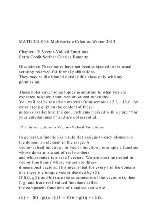
12-2 Chapter 12: Vector-Valued Functions
Figure 12.1: Visualization of Limits for Vector Functions
lim
t→a
r(t) = L. (12.1)
One way to motivate a reasonable definition of (12.1) is to
position r(t) and L with their initial points at the
origin and interpret this limit to mean that the terminal point of
r(t) approaches the terminal point of L as t
approaches a or, equivalently, that the vector r(t) approaches the
vector L in both length and direction as t
approaches a (Figure 12.1). Algebraically, this is equivalent to
stating that
lim
t→a
||r(t)− L|| = 0 (12.2)
(Figure 12.1). Thus, we make the following definition.
Definition 12.2 Let r(t) be a vector function that is defined for
all t in some open interval containing the
number a, except that r(t) need not be defined at a. We will
write
lim
t→a
4. r(t) = L
if and only if
lim
t→a
||r(t)− L|| = 0.
Theorem 12.3 If r has a limit at a, then this limit is unique.
Proof: Suppose that r has limits L1 and L2 at a. Let � > 0 be
given, but fixed. Then there exist δ1, δ2 > 0
such that ||r(t) − L1|| < �/2 whenever 0 < |t − a| < δ1 and ||r(t) −
L1|| < �/2 whenever 0 < |t − a| < δ2.
Hence, for each t such that 0 < |t− a| < min{δ1, δ2},
Chapter 12: Vector-Valued Functions 12-3
||L1 − L2|| =
∣ ∣ ∣ ∣ ((L1 − r(t)) + (r(t)− L2)∣ ∣ ∣ ∣ ≤ ||r(t)− L1||+ ||r(t)− L2||
≤ �
2
+
�
2
= �.
Yet � was arbitrary, and so ||L1 −L2|| is a nonnegative number
that is smaller than every positive number �.
It follows that ||L1 − L2|| = 0, and so L1 = L2, making the limit
unique.
5. It is clear intuitively that r(t) will approach a limiting vector L
as t approaches a if and only if the
component functions of r(t) approach the corresponding
components of L. This suggests the following.
Theorem 12.4 (a) If r(t) = 〈x(t), y(t)〉, then
lim
t→a
r(t) =
⟨
lim
t→a
x(t), lim
t→a
y(t)
⟩
provided the limits of the component functions exist.
Conversely, the limits of the component functions
exist provided r(t) approaches a limiting vector as t approaches
a.
(b) If r(t) = 〈x(t), y(t), z(t)〉, then
lim
t→a
r(t) =
⟨
6. lim
t→a
x(t), lim
t→a
y(t), lim
t→a
z(t)
⟩
provided the limits of the component functions exist.
Conversely, the limits of the component functions
exist provided r(t) approaches a limiting vector as t approaches
a.
Proof: We will only prove part (a), as the proof of part (b) is
virtually identical. Suppose that lim
t→a
x(t) = L1
and lim
t→a
y(t) = L2. Then
lim
t→a
||r(t)−〈L1, L2〉|| = lim
t→a
√
(x(t)− L1)2 + (y(t)− L2)2 =
8. y(t)
⟩
Conversely, suppose that lim
t→a
r(t) = 〈L1, L2〉. Then
0 ≤ |x(t)− L1| =
√
(x(t)− L1)2 ≤
√
(x(t)− L1)2 + (y(t)− L2)2 = ||r(t)− 〈L1, L2〉|| → 0
as t→ a. It follows by the Squeeze Theorem that lim
t→a
x(t) = L1. The same reasoning begets lim
t→a
y(t) = L2.
Limits of vector functions obey the same rules as limits of real-
valued functions. This is a trivial
consequence of Theorem 12.4, so we omit the proof.
12-4 Chapter 12: Vector-Valued Functions
Figure 12.2: C is traced out by the tip of a moving position
vector r(t).
Proposition 12.5 Suppose u and v are vector functions that
possess limits as t approaches a and let c be
9. a scalar. Then the following properties hold.
(a) lim
t→a
[u(t)± v(t)] = lim
t→a
u(t)± lim
t→a
v(t)
(b) lim
t→a
cu(t) = c lim
t→a
u(t)
(c) lim
t→a
[u(t) •v(t)] = lim
t→a
u(t) • lim
t→a
v(t)
(d) lim
t→a
[u(t)× v(t)] = lim
10. t→a
u(t)× lim
t→a
v(t)
Example 12.6 According to Theorem 12.4, if r(t) = (1 + t3)i +
te–tj +
sin t
t
k, then
lim
t→0
r(t) =
[
lim
t→0
(1 + t3)
]
i +
[
lim
t→0
te–t
]
j +
[
lim
t→0
11. sin t
t
]
k = i + k.
Definition 12.7 A vector function r is continuous at a if
lim
t→a
r(t) = r(a). (12.3)
In the case where r is continuous on R, we will say that r is
continuous everywhere, or just continuous.
In view of Definition 12.2, we see that r is continuous at a if
and only if its component functions f, g,
and h are continuous at a. Additionally, for any real-valued
function F (t), lim
t→a
r(F (t)) = r
(
lim
t→a
F (t)
)
.
There is a close connection between continuous vector functions
12. and space curves. Suppose that f, g, and
h are continuous real-valued functions on an interval I. Then the
set C of all points (x, y, z) in space, where
x = f(t), y = g(t), z = h(t), (12.4)
and t varies throughout the interval I, is called a space curve .
The equations in (12.4) are called parametric
equations of C , and t is called a parameter . We can think of C
as being traced out by a moving particle
Chapter 12: Vector-Valued Functions 12-5
whose position at time t is (f(t), g(t), h(t)). If we now consider
the vector function r(t) = 〈f(t), g(t), h(t)〉,
then r(t) is the position vector of the point P (f(t), g(t), h(t)) on
C. Thus, any continuous vector function r
defines a space curve C that is traced out by the tip of the
moving vector r(t), as shown in Figure 12.2.
Example 12.8 Let us find a vector function that represents the
curve of intersection of the cylinder
x2 + y2 = 1 and the plane y + z = 2. The projection of C onto
the xy-plane is the circle x2 + y2 = 1, z = 0.
So we know that we can write
x = cos t, y = sin t, t ∈ R.
From the equation of the plane, we have
z = 2− y = 2− sin t.
So we can write parametric equations for C as
13. x = cos t, y = sin t, z = 2− sin t, t ∈ R.
The corresponding vector equation is
r(t) = cos ti + sin tj + (2− sin t)k.
This equation is called a parametrization of the curve C.
12.2 Calculus of Vector-Valued Functions
In this section, we will define derivatives and integrals of
vector functions and discuss their properties.
12.2.1 Derivatives
The derivative of a vector function is defined in much the same
way as for real-valued functions.
Definition 12.9 If r is a vector function, we define the
derivative of r with respect to t to be the vector
function r′ given by
r′(t) = lim
h→0
r(t+ h)− r(t)
h
. (12.5)
The domain of r′ consists of all values of t in the domain of r(t)
for which the limit exists. The function r(t)
is differentiable at t if the limit in (12.5) exists. All of the
standard notations for derivatives still apply.
14. 12-6 Chapter 12: Vector-Valued Functions
Figure 12.3: Geometric Interpretation of the Derivative
Theorem 12.10 If r is differentiable at a, then r is continuous at
a.
Proof: We have r(t)− r(a) = r(t)− r(a)
t− a
· (t− a)→ r′(a) · 0 = 0 as t→ a. Therefore lim
t→a
r(t) = r(a).
The geometric significance of this definition is shown in parts
(a) and (b) of Figure 12.3. These illustrations
show the graph C of r(t) (with its orientation) and the vectors
r(t), r(t+ h), and r(t+ h)− r(t) for positive
h and negative h. In both cases, the vector r(t+ h)− r(t) runs
along the secant line joining the terminal
points of r(t+ h) and r(t), but with opposite directions in the two
cases. In the case where h > 0, the vector
r(t+ h)− r(t) points in the direction of increasing t, and in the
case where h < 0, it points in the opposite
direction. However, in the case where h < 0, the direction gets
reversed when we multiply by 1/h. So in
both cases, the scalar multiple (1/h)[r(t+ h)− r(t)] points in the
direction of increasing t and runs along the
secant line. As h→ 0, it appears that this vector approaches a
vector that lies on the tangent line.
The following theorem gives us a convenient method for
computing the derivative of a vector function r :
just differentiate each component of r.
15. Theorem 12.11 If r(t) is a vector function, then r is
differentiable at t if and only if each of its component
functions is differentiable at t, in which case the component
functions of r′(t) are the derivatives of the
corresponding component functions of r(t).
Proof: For simplicity, we give the proof in 2-space; the proof in
3-space is identical, except for the additional
component. Assume that r(t) = 〈x(t), y(t)〉. Then
Chapter 12: Vector-Valued Functions 12-7
Figure 12.4: The Tangent Vector and the Tangent Line
r′(t) = lim
h→0
r(t+ h)− r(t)
h
= lim
h→0
1
h
[〈x(t+ h), y(t+ h)〉 − 〈x(t), y(t)〉]
= lim
h→0
⟨
x(t+ h)− x(t)
16. h
,
y(t+ h)− y(t)
h
⟩
=
⟨
lim
h→0
x(t+ h)− x(t)
h
, lim
h→0
y(t+ h)− y(t)
h
⟩
= 〈x′(t), y′(t)〉.
Example 12.12 The derivative of r(t) = (1 + t3)i + te–tj + sin 2tk
is
r′(t) = 3t2i + (1− t)e–tj + 2 cos 2tk.
Motivated by the discussion of the geometric interpretation of
the derivative of a vector function, we
make the following definition.
Definition 12.13 Let P be a point on the graph of a vector
17. function r(t), and let r(t0) be the radial vector
from the origin to P (Figure 12.6). If r′(t0) exists and r
′(t0) 6= 0, then we call r′(t0) the tangent vector to
the graph of r(t) at r(t0), and we call the line P that is parallel to
the tangent vector the tangent line to
the graph of r(t) at r(t0).
Let r0 = r(t0) and v0 = r
′(t0). It follows that the tangent line to the graph of r(t) at r0 is
given by the
vector equation
r = r0 + tv. (12.6)
12-8 Chapter 12: Vector-Valued Functions
Example 12.14 Suppose we want to find the tangent line to the
helix to with parametric equations
x = 2 cos t, y = sin t, z = t
at the point (0, 1, π/2) is the line through the point. Its vector
equation is r(t) = 〈2 cos t, sin t, t〉, so
r′(t) = 〈–2 sin t, cos t, 1〉.
The parameter value corresponding to the point (0, 1, π/2) is t =
π/2, so the tangent vector there is
r′(π/2) = 〈–2, 0, 1〉. The tangent line is the line through (0, 1,
π/2) parallel to the vector 〈–2, 0, 1〉, so its
parametric equations are
18. x = –2t, y = t, z =
π
2
+ t.
Just as for real-valued functions, the second derivative of a
vector function r is the derivative of r′,
that is, r′′ = r′. For instance, the second derivative of the
function in Example 12.13 is
r′′(t) = 〈–2 cos t, – sin t, 0〉.
Definition 12.15 A curve given by a vector function r(t) on an
interval I is called smooth if r′ is continuous
and r′(t) 6= 0, except possible at the endpoints of I.
For instance, the helix in Example 12.13 is smooth because r′(t)
is never 0.
Example 12.16 The semi cubical parabola r(t) = 〈1 + t3, t2〉 is
not smooth, because
r′(t) = 〈3t2, 2t〉,
and so r′(0) = 〈0, 0〉 = 0. To see the behavior of r from a Calc
I perspective, note that the parametric
equations of r satisfy y = (x− 1)2/3 so that dy/dx = (2/3)(x− 1)–
1/3 for x 6= 1, which is also the point at
which t = 0. Observe that lim
x→1−
(2/3)(x − 1)–1/3 = –∞ whereas lim
x→1+
(2/3)(x − 1)–1/3 = +∞. This tells us
19. that there is a sharp corner, called a cusp, at (1, 0). Any curve
with this type of behavior—an abrupt change
in direction—is not smooth.
A curve, such as the semi cubical parabola, that is made up of a
finite number of smooth pieces is called
piecewise smooth .
The next theorem shows that the differentiation formulas for
real valued functions have their counterparts
for vector-valued functions.
Theorem 12.17 Suppose u and v are differentiable vector
functions, k is a scalar, c is a constant vector,
and f is a real-valued function. Then
Chapter 12: Vector-Valued Functions 12-9
(a)
d
dt
[c] = 0
(b)
d
dt
[ku(t)] = ku′(t)
(c)
d
20. dt
[u(t)± v(t)] = u′(t)± v′(t)
(d)
d
dt
[f(t)u(t)] = f ′(t)u(t) + f(t)u′(t)
(e)
d
dt
[u(t) •v(t)] = u′(t) •v′(t) + u(t) •v(t)
(f)
d
dt
[u(t)× v(t)] = u′(t)× v(t) + u(t)× v′(t)
(g)
d
dt
[u(f(t))] = f ′(t)u′(f(t))
Proof: Formulas (a)-(d) and (g) (the chain rule) can be proved
by using Theorem 12.10 and the corresponding
differentiation formulas for real-valued functions. Formulas (e)
and (f) can be seen more readily by applying
Definition 12.9 directly. The proof of (e) is included here due to
its importance. Indeed
d
23. v(t+ h)− v(t)
h
)
= u′(t) •v(t) + u(t) •v′(t).
The proof of Formula (f) is the same. Just replace each • with ×.
Corollary 12.18 If r is a differentiable vector function and ||r(t)||
is constant for all t, then
r(t) • r′(t) = 0, (12.7)
that is, r(t) and r′(t) are orthogonal vectors for all t.
12-10 Chapter 12: Vector-Valued Functions
Figure 12.5: Orthogonality of r(t) and r′(t) for Curves on the
Surface of a Sphere
Proof: Suppose that ||r(t)|| = c, where c is a constant. Since
||r(t)||2 = c2 and c2 is a constant, Formula (e)
of Theorem 12.17 gives
0 =
d
dt
[||r(t)||2] d
dt
[r(t) • r(t)] = r′(t) • r(t) + r(t) • r′(t) = 2r(t) • r′(t).
Thus r(t) • r′(t) = 0.
24. Geometrically, this result says that if a curve lies on a sphere
with center the origin, then the tangent
vector r′(t) is always orthogonal to the position vector r(t)
(Figure 12.5).
12.2.2 Integrals
The definite integral of a continuous vector function r can be
defined in much the same way as for
real-valued functions expect that the integral is a vector. (We
use the notation of Chapter 5.)
Definition 12.19 A continuous vector function r is said to be
integrable on a finite closed interval [a, b]
if the limit
lim
max ∆tk→0
n∑
k=1
r(t∗ k)∆tk
exists and does not depend on the choice of partitions or on the
choice of the points x∗ k in the subintervals.
When this is the case, we denote the limit by
∫ b
a
r(t) dt = lim
max ∆tk→0
n∑
25. k=1
r(t∗ k)∆tk (12.8)
Chapter 12: Vector-Valued Functions 12-11
which is called the definite integral of r from a to b. The
numbers a and b are called the lower limit of
integration and the upper limit of integration, respectively, and
r(t) is called the integrand.
But then we can express the integral of r in terms of the
integrals of its component functions f, g, and h.
For example, if r(t) = 〈x(t), y(t)〉, then
∫ b
a
r(t) dt = lim
max ∆tk→0
n∑
k=1
r(t∗ k)∆tk
= lim
max ∆tk→0
n∑
k=1
〈x(t), y(t)〉∆tk
27. ∫ b
a
y(t) dt
⟩
.
This begets the following theorem.
Theorem 12.20 If r is a continuous vector function on a finite
closed interval [a, b], then r is integrable on
[a, b] if and only if each of its component functions is
integrable on [a, b], in which case the components of∫ b
a
r(t) dt are the definite integrals of the corresponding component
functions of r(t).
As with differentiation, many of the rules for integrating real-
valued functions have analogs for vector
functions. We omit the proof of the following proposition, as
each fact follows trivially from Theorem 12.20
Proposition 12.21 Let u and v be continuous vector functions on
[a, b], and let k be a scalar. Then
(a)
∫ b
a
ku(t) dt = k
∫ b
a
28. u(t) dt
(b)
∫ b
a
[u(t)± v(t)] dt =
∫ b
a
u(t) dt±
∫ b
a
v(t) dt
We can extend the Fundamental Theorem of Calculus to
continuous vector functions as follows:
∫ b
a
r(t) dt = R(t)
∣ ∣ ∣ ∣ ∣
b
a
= R(b)−R(a), (12.9)
where R is an antiderivative of r, that is, R′(t) = r(t). We use the
notation
∫
29. r(t) dt for indefinite
integrals (antiderivatives).
Example 12.22 If r(t) = 2 cos ti + sin tj + 2tk, then
12-12 Chapter 12: Vector-Valued Functions
∫
r(t) dt =
(∫
2 cos t dt
)
i +
(∫
sin t dt
)
j +
(∫
2t dt
)
k = 2 sin ti− cos tj + t2k + C,
where C is a vector constant of integration, and
∫ π/2
0
30. r(t) dt =
[
2 sin ti− cos tj + t2k
]π/2
0
= 2i + j +
π2
4
k
Unfortunately, our standard intuitive understanding of the
definite integral as the ‘‘net signed area
under a curve’’ makes no sense here, since any reasonable
interpretation of ‘‘signed area’’ would be scalar,
whereas the integral of a vector function is always a vector. Our
interpretation of vector functions as position
functions fares no better, since while we have interpretations
for the integrals of velocity and acceleration,
we do not have a physical interpretation of the integral of
position. Nevertheless, we can still relate some
important aspects of a space curve with vector-valued
integration. The first of which is the displacement
vector from r(a) to r(b), that is, the vector starting at the point
on the curve corresponding to t = a and
ending at the point corresponding to t = b, which can be
determined by integrating the velocity function:
[
displacement vector
from t = a to t = b
]
=
31. ∫ b
a
r′(t) dt = r(b)− r(a).
Note that this is just the Fundamental Theorem of Calculus
applied to a vector function. We investigate
another application in the next section.
12.3 Change of Parameter; Arc Length
We observed in the past that a curve in 2-space or 3-space
permit multiple parametrizations. Sometimes it is
desirable to change the parameter for a parametric curve to a
different parameter that is better suited for
the problem at hand. In this section, we will investigate issues
associated with changes of parameter, and we
will show that arc length plays a special role in parametric
representations of curves.
12.3.1 Arc Length from the Vector Viewpoint
In Calc II, we define the length of a plane curve with parametric
equations x = f(t), y = g(t), a ≤ t ≤ b, as
the limit of lengths of inscribed triangulations and, for the case
where f ′ and g′ are continuous on [a, b], we
arrived at the formula
L =
∫ b
a
√(
dx
32. dt
)2
+
(
dy
dt
)2
dt. (12.10)
The length of a smooth space curve is defined in exactly the
same way.
Definition 12.23 Suppose that a smooth space curve C has the
vector equation r(t) = 〈f(t), g(t), g(t)〉,
a ≤ t ≤ b, where f ′, g′, and h′ are continuous on [a, b]. If C is
traversed exactly once as t increases from a
to b, then its arc length is
Chapter 12: Vector-Valued Functions 12-13
L =
∫ b
a
√(
dx
dt
33. )2
+
(
dy
dt
)2
+
(
dz
dt
)2
dt. (12.11)
Notice that both of the arc length formulas (12.10) and (12.11)
can be put into the more compact form
L =
∫ b
a
||r′(t)|| dt (12.12)
because for plane curves r(t) = 〈x(t), g(t)〉,
||r′(t)|| =
∣ ∣ ∣ ∣ ∣ ∣ ∣ ∣ ⟨ dxdt , dydt
⟩ ∣ ∣ ∣ ∣ ∣ ∣ ∣ ∣ =
35. )2
+
(
dz
dt
)2
.
Example 12.24 For the circular helix with vector equation r(t) =
cos ti + sin tj + tk, we have
||r′(t)|| =
√
(– sin t)2 + cos2t+ 1 =
√
2.
The arc from (1, 0, 0) to (1, 0, 2π) is described by the parameter
interval 0 ≤ t ≤ 2π, and so, from Formula
(12.12), we have
L =
∫ 2π
0
||r′(t)|| dt =
∫ 2π
0
36. √
2 dt = 2
√
2π.
12.3.2 Arc Length as a Parameter
A single curve C can be represented by more then one vector
function. For instance, the twisted cubic
r1(t) = 〈t, t2, t3〉 1 ≤ t ≤ 2 (12.13)
can also be represented by the function
r2(u) = 〈eu, e2u, e3u〉 0 ≤ u ≤ ln 2 (12.14)
12-14 Chapter 12: Vector-Valued Functions
where the connection between the parameters t and u is given by
t = eu. We say that Equations (12.13)
and (12.14) are parametrizations of the curve C. If we use
Equation (12.12) to compute the arc length of
C using Equations (12.13) and (12.14), we get the same answer.
(Check this!) In general, when Equation
(12.12) is used to compute the length of any piecewise-smooth
curve, the arc length is independent of the
parametrization that is used.
Theorem 12.25 The arc length of a smooth curve is independent
of its parametrization.
Proof: Let r1 and r2 be two smooth parametrizations of a curve
37. C on the finite closed intervals [a, b] and
[α, β], respectively, where r1([a, b]) = r2([α, β]). Since r1 and
r2 are parametrizations of the same curve, it
follows that r1(b) = r2(β) and for every u ∈ [α, β], there exists a
unique t ∈ [a, b] such that r2(s) = r1(t).
Thus, there is an invertible function f : [α, β]→ [a, b] so that
r2(u) = r1(f(u)). Since r1 and r2 are smooth,
the Inverse Function Theorem and the Chain Rule dictate that f
is continuously differentiable on [α, β], and
r2
′(u) =
d
du
[r1(f(u))] = f
′(u)r′1(f(u)).
Since f is invertible and differentiable, f is strictly increasing,
and so f ′(u) > 0 on [α, β]. To finish the proof,
we have
∫ β
α
||r′2(u)|| du =
∫ β
α
||f ′(u)r′1(f(u))|| du =
∫ β
α
||r′1(f(u))||f ′(u) du
38. since f ′(u) is a positive scalar. Making the substitution t = f(u),
we have dt = f ′(u) du so that
∫ β
α
||r′1(f(u))||f ′(u) du =
∫ f(β)=b
f(α)=a
||r′1(t)|| dt,
both of which give the arc length of C.
Definition 12.26 Suppose that C is a piecewise-smooth curve
given by a vector function r(t), a ≤ t ≤ b,
and C is traversed exactly once as t increases from a to b. We
define its arc length function s by
s(t) =
∫ t
a
||r′(u)|| du (12.15)
Thus s(t) is the length of the part of C between r(a) and r(t).
(See Figure 12.6.) The point on C given by
r(a) is called the reference point . If we differentiate both sides
of Equation (12.15) using the Fundamental
Theorem of Calculus, we obtain
ds
dt
39. = ||r′(t)|| (12.16)
Chapter 12: Vector-Valued Functions 12-15
Figure 12.6: The Arc Length Function
Theorem 12.27 (a) If C is the graph of a smooth vector function
r, where t is a general parameter, and if
s is the arc length parameter for C defined by Formula (12.12),
then for every value of t the tangent
vector has length ∣ ∣ ∣ ∣ ∣ ∣ ∣ ∣ drdt
∣ ∣ ∣ ∣ ∣ ∣ ∣ ∣ = dsdt (12.17)
(b) If C is the graph of a smooth vector function r, where s is an
arc length parameter, then for every value
of s the tangent vector to C has length ∣ ∣ ∣ ∣ ∣ ∣ ∣ ∣ drds
∣ ∣ ∣ ∣ ∣ ∣ ∣ ∣ = 1 (12.18)
(c) If C is the graph of a smooth vector function r, and if
||dr/dt|| = 1 for every value of t, then for any
value of t0 in the domain of r, the parameter s = t− t0 is an arc
length parameter that has its reference
point at the point on C where t = t0.
Proof:
(a) See the paragraph preceding Theorem 12.27.
(b) Let t = s in part (a).
(c) It follows from Formula (12.12) that the formula
s =
40. ∫ t
t0
∣ ∣ ∣ ∣ ∣ ∣ ∣ ∣ drdu
∣ ∣ ∣ ∣ ∣ ∣ ∣ ∣ du
defines an arc length parameter for C with reference point r(0).
However ||dr/du|| = 1 by hypothesis, so
we can rewrite the formula for s as
12-16 Chapter 12: Vector-Valued Functions
s =
∫ t
t0
du = t− t0.
It is often useful to parametrize a curve with respect to arc
length because arc length arises naturally
from the shape of the curve and does not depend on a particular
coordinate system. If a curve r(t) is already
given in terms of a parameter t and s(t) is the arc length
function given by Equation (12.15), then we may
be able to solve for t as a function of s: t = t(s). Then the curve
can be reparametrized in terms of s by
substituting for t : r = r(t(s)). Thus, if s = 3 for instance, r(t(3))
is the position vector of the point 3 units
of length along the curve from its reference point.
Example 12.28 We wish to reparametrize the helix r(t) = cos ti
+ sin tj + tk with respect to arc length
41. measured from (1, 0, 0) in the direction of increasing t. The
reference point (1, 0, 0) corresponds to the
parameter t = 0. From Example 12.24, we have
ds
dt
= ||r′(t)|| =
√
2,
and so
s = s(t) =
∫ t
0
r′(u)|| du =
∫ t
0
√
2 du =
√
2t.
Therefore t = s/
√
2 and the required reparametrization is obtained by substituting
for t :
42. r(s) = cos
(
s√
2
)
i + sin
(
s√
2
)
j +
s√
2
k.
Example 12.29 A bug walks along the trunk of a tree following
a path modeled by the circular helix in
Example 12.28. The bug starts at the reference point (1, 0, 0)
and walks up the helix for a distance of 10
units. To find the bug’s final coordinates, it suffices to set s =
10 into our answer in Example 12.28 so that
its final coordinates are
(
cos
(
10√
2
43. )
, sin
(
10√
2
)
,
10√
2
)
.
Proposition 12.30 Let r(t) = r0 + tv be the vector equation of a
line that passes through the terminal point
r0 and is parallel to the vector v. The arc length parametrization
of the line that has reference points r0 and
the same orientation as r is
r(s) = r0 + s
(
v
||v||
)
. (12.19)
Proof: Note that r(0) = r0, the reference point, and dr/dt = v.
Hence
44. Chapter 12: Vector-Valued Functions 12-17
s =
∫ t
0
||r′(u)|| du =
∫ t
0
||v|| du = t||v||.
This implies that t = s/||v||, and the reparametrization now
follows.
Example 12.31 We wish to find the arc length parametrization
of the line
x = 2t+ 1, y = 3t− 2
that has the same orientation as the given line and uses (1, –2)
as the reference point. Observe that the line
is parallel to v = 2i + 3j. To find the arc length parametrization
of the line, we need only rewrite the given
equation using v/||v|| rather than v to determine the direction
and replace t by s. Since
v
||v||
=
45. 2i + 3j√
13
=
2√
13
i +
3√
13
j,
it follows that the parametric equations for the line in terms of s
are
s =
2√
13
s+ 1, y =
3√
13
s− 2.
? A cable has radius r and length L and is wound around a spool
with radius R without overlapping. What
is the shortest length along the spool that is covered by the
cable?
12.4 Unit Tangent, Normal, and Binormal Vectors
In this section, we will discuss some of the fundamental
geometric properties of vector functions. Our work
here will have important applications to the study of motion
along a curved path in 2-space or 3-space and
46. to the study of the geometric properties of curves and surfaces.
12.4.1 Unit Tangent Vectors
Definition 12.32 Let C be the graph of a smooth vector function
r(t) so that the vector r′(t) is nonzero,
tangent to C, and points in the direction of increasing
parameter. Thus, by normalizing r′(t), we obtain a
unit vector
T(t) =
r′(t)
||r′(t)||
(12.20)
that is tangent to C and points in the direction of increasing
parameter t. We call T(t) the unit tangent
vector to C at t.
12-18 Chapter 12: Vector-Valued Functions
Figure 12.7: Vectors Orthogonal to T(t)
Example 12.33 Let r(t) = 2ti + t2j + t2k. Then r′(t) = 2i + 2tj +
2tk, and so the unit tangent vector to
graph of r(t) at the point where t = 2 is
T(2) =
r′(2)
||r′(2)||
=
47. 2i + 4j + 4k√
36
=
2i + 4j + 4k
6
=
1
3
i +
2
3
j +
2
3
k.
12.4.2 Unit Normal Vectors
At a given point on a smooth curve r(t), there are multiple
vectors that are orthogonal to the unit tangent
vector T(t) (Figure 12.7). We single out one by observing that,
because ||T(t)|| = 1 for all t, we have
T(t) •T′(t) = 0 for all t by Corollary 12.18. So T′(t) is
orthogonal to T(t). Note that T′(t) is not necessarily
a unit vector, but if r′ is also smooth, we can obtain one that
points in the same direction as T′(t).
Definition 12.34
48. If r and r′ are smooth curves, then we define the principal unit
normal vector N(t) (or simply unit
normal) at t as
N(t) =
T′(t)
||T′(t)||
(12.21)
We can think of the normal vector as indicating the direction in
which the curve is turning at each point.
Example 12.35 Consider the circular helix r(t) = a cos ti+a sin
tj+ctk, where a > 0, c is a constant. Then
Chapter 12: Vector-Valued Functions 12-19
Figure 12.8: Unit Normal Pointing Towards the z-Axis
r′(t) = –a sin ti + a cos tj + ck
||r′(t)|| =
√
(–a sin t)2 + (a cos t)2 + c2 =
√
a2 + c2
T(t) =
r′(t)
||r′(t)||
49. = –
a sin t√
a2 + c2
i +
a cos t√
a2 + c2
j +
c√
a2 + c2
k
T′(t) = –
a cos t√
a2 + c2
i− a sin t√
a2 + c2
j
||T′(t)|| =
√(
–
a cos t√
a2 + c2
)2
+
(
50. a sin t√
a2 + c2
)2
=
√
a2
a2 + c2
=
a√
a2 + c2
N(t) =
T′(t)
||T′(t)||
= – cos ti− sin tj = –(cos ti + sin tj)
Note that the k component of the unit normal N(t) is zero for
every value of t, so this vector always lies in a
horizontal plane, as illustrated in Figure 12.8. We leave it as an
exercise to show that this vector actually
always point toward the z-axis.
Our next objective is to show that for a nonlinear parametric
curve C in 2-space the unit normal always
points toward the concave side of C. For this purpose, let φ(t)
be the angle from the positive x-axis to T(t),
and let n(t) be the unit vector that results from rotating T(t)
counterclockwise through an angle of π/2
(Figure 12.9). Since T(t) and n(t) are unit vectors, it follows
that these vectors can be expressed as
51. T(t) = cosφ(t)i + sinφ(t)j (12.22)
and
n(t) = cos
(
φ(t) +
π
2
)
i + sin
(
φ(t) +
π
2
)
j = – sinφ(t)i + cosφ(t)j. (12.23)
12-20 Chapter 12: Vector-Valued Functions
Figure 12.9: Angle of Inclination Function φ(t)
Observe that on intervals where φ(t) is increasing the vector n(t)
points toward the concave side of C, and
on intervals where φ(t) is decreasing it points away from the
concave side (Figure 12.9).
52. Now let us differentiate T(t) by using Formula (12.22) and
applying the chain rule. This yields
dT
dt
=
dT
dφ
dφ
dt
= [(– sinφ)i + (cosφ)j]
dφ
dt
,
and thus from Formula (12.23)
dT
dt
= n(t)
dφ
dt
. (12.24)
Yet dφ/dt > 0 on intervals where φ(t) is increasing and dφ/dt < 0
on intervals where φ(t) is decreasing.
It thus follows from Formula (12.24) that dT/dt has the same
53. direction as n(t) on intervals where φ(t) is
increasing and the opposite direction on intervals where φ(t) is
decreasing. Therefore T′(t) points ‘‘inward’’
toward the concave side of the curve at all times, and hence so
does N(t). For this reason, N(t) is also called
the inward unit normal when applied to curves in 2-space.
In the case where r(s) is parametrized by arc length, the
procedures for computing T(s) and N(s) can
be simplified. For example, Theorem 12.27 says that if s is an
arc length parameter, then ||r′(s)|| = 1, and so
T(s) = r′(s) (12.25)
and
N(s) =
r′′(s)
||r′′(s)||
. (12.26)
Example 12.36 The circle of radius a with counterclockwise
orientation and centered at the origin can be
represented by the vector function
Chapter 12: Vector-Valued Functions 12-21
Figure 12.10: Unit Tangent and Unit Normal of a Circle
r(t) = a cos ti + a sin tj (0 ≤ t ≤ 2π)
We can interpret t as the angle in radian measure from the
positive x-axis to the radius vector. From basic
54. precalculus, this angle subtends an arc of length s = at on the
circle, so we can reparametrize the circle in
terms of s by substituting s/a for t. This yields
r(s) = a cos
( s
a
)
i + a sin
( s
a
)
j (0 ≤ s ≤ 2πa).
Hence
T(s) = r′(s) = – sin
( s
a
)
i + cos
( s
a
)
j
r′′(s) = –
1
a
56. a
)]2
=
1
a
N(s) =
r′′(s)
||r′′(s)||
= – cos
( s
a
)
i− sin
( s
a
)
j
so N(s) points toward the center of the circle for all s (Figure
12.10). This makes sense geometrically and is
also consistent with our earlier observation that in 2-space the
unit normal points inward.
12-22 Chapter 12: Vector-Valued Functions
57. Figure 12.11: Right-Hand Rule Orientation of T, N, and B
12.4.3 Binormal Vectors
Definition 12.37 If C is the graph of a vector-valued function
r(t) in 3-space, then we define the binormal
vector to C at t to be
B(t) = T(t)×N(t) (12.27)
Note that if T and N are parametrized with respect to arc length
s, then
B(s) = T(s)×N(s) = r′(s)× r
′′(s)
||r′′(s)||
=
r′(s)× r′′(s)
||r′′(s)||
.
By the definition of the cross product, B is orthogonal to both T
and N and is oriented relative to T
and N by the right-hand rule. Moreover, B(t) is a unit vector
since
||B(t)|| = ||T(t)×N(t)|| = ||T(t)|| ||N(t)|| sin
(π
2
)
= 1.
58. Thus {T(t),N(t),B(t)} is a set of mutually orthogonal unit
vectors. (More can be said actually. Like i,
j, and k, the vectors T(t), N(t), and B(t) determine a right-
handed coordinate system in 3-space (Figure
12.11). We will see why shortly.)
Example 12.38 Consider the circular helix r(t) = a cos ti + a sin
tj + ctk, where a > 0, c is a constant.
In Example 12.35, we found that T(t) = (–a sin t/
√
a2 + c2)i + (a cos t/
√
a2 + c2)j + (c/
√
a2 + c2)k and
N(t) = –(cos ti + sin tj). The binormal vector is
B(t) = T(t)×N(t) = 1√
a2 + c2
∣ ∣ ∣ ∣ ∣ ∣
i j k
–a sin t a cos t c
– cos t – sin t 0
∣ ∣ ∣ ∣ ∣ ∣ = c sin t√a2 + c2 i− c cos t√a2 + c2 j + a
2
√
a2 + c2
59. k.
Chapter 12: Vector-Valued Functions 12-23
Figure 12.12: The Frenet Frame
Not only are T(t), N(t), and B(t) mutually orthogonal unit
vectors, but each vector is related to the
other two by the right-hand rule. Indeed, using the formula a×
(b× c) = (a • c)b− (a •b)c,
T×N = B
N×B = N× (T×N) = (N •N)T− (N •T)N = ||N||2T− 0N = T
B×T = B× (N×B) = (B •B)N− (B •N)B = ||B||2N− 0B = N
The coordinate system determined by T(t), N(t), and B(t) is
called the TNB-frame or Frenet frame.
Whereas the xyz-coordinate system determined by i, j, and k
remains fixed, the Frenet frame changes as
its origin moves along the curve C (Figure 12.12).
At each point on a smooth curve given parametric equations r(t)
= 〈x(t), y(t), z(t)〉 in 3-space, the
vectors T(t), N(t), and B(t) determine three mutually
perpendicular planes that pass through the point
(x(t), y(t), z(t)). They are the TB-plane (called the rectifying
plane), the TN-plane (called the osculating
plane), and the NB-plane (called the normal plane) (Figure
12.13). The osculating plane is especially
important as it is the plane that comes closest to containing the
part of the curve near (x(t), y(t), z(t)). (For
a plane curve, the osculating plane is simply the plane that
contains the curve.) The name comes from the
60. Latin osculum, meaning ‘‘kiss.’’
Example 12.39 Let us find the equations of the rectifying,
osculating, and normal planes of the helix in
Example 12.38 at the point P (0, a, cπ/2). Note that r(t) = a cos
ti + a sin tj + ctk passes through P when
t = π/2. The rectifying plane at P contains the vectors T(π/2)
and B(π/2), so its normal vector is N(π/2).
So
N(t) = –(cos ti + sin tj)⇒ N
(π
2
)
= –j.
So an equation of the rectifying plane is
–(y − a) = 0 or y = a.
The osculating plane at P contains the vectors T(π/2) and
N(π/2), so its normal vector is B(π/2). So
B(t) =
c sin t√
a2 + c2
i− c cos t√
a2 + c2
j +
a2√
a2 + c2
61. k⇒ B
(π
2
)
=
c√
a2 + c2
i +
a2√
a2 + c2
k.
12-24 Chapter 12: Vector-Valued Functions
Figure 12.13: The Rectifying, Osculating, and Normal Planes
A simpler normal vector is 〈c, 0, a2〉, so an equation of the
osculating plane is
cx+ a2
(
z − π
2
)
= 0 or z = –
c
62. a2
x+
π
2
Lastly, the normal plane at P has normal vector r′(π/2) = 〈–a, 0,
c〉, so an equation of it is
–ax+ c
(
z − π
2
)
= 0 or z =
a
c
x+
π
2
.
12.5 Curvature
If C is a smooth curve, then we can use the derivative dT/ds to
measure the ‘‘bendiness’’ of a curve. We
formalize this idea by considering the curvature of a curve. The
curvature of C at a given point is a measure
63. of how quickly the curve changes direction at that point.
Specifically, we define it to be the magnitude of the
rate of change of the unit tangent vector with respect to arc
length. (We use arc length so that the curvature
is independent of the parametrization.)
12.5.1 Definition and Formulas for Curvature
Definition 12.40 The curvature of a smooth curve in 2-space or
3-space that is parametrized by arc
length is
κ(s) =
∣ ∣ ∣ ∣ ∣ ∣ ∣ ∣ dTds
∣ ∣ ∣ ∣ ∣ ∣ ∣ ∣ = ||r′′(s)|| (12.28)
Chapter 12: Vector-Valued Functions 12-25
where T is the unit tangent vector.
We can even express N(s) and B(s) in terms of curvature:
N(s) =
r′′(s)
||r′′(s)||
=
r′′(s)
κ(s)
=
64. 1
κ(s)
dT
ds
(12.29)
B(s) =
r′(s)× r′′(s)
||r′′(s)||
=
r′(s)× r′′(s)
κ(s)
. (12.30)
Is this a good definition for curvature though? Let us put it to
the test.
Proposition 12.41 All lines have zero curvature.
Proof: Recall from Proposition 12.30 that a line in 2-space or 3-
space can be parametrized in terms of arc
length as
r(s) = r0 + su
where the terminal point of r0 is a point on the line and u is a
unit vector parallel to the line. Since r0
and u are constant, their derivatives with respect to s are zero,
and hence r′(s) = u and r′′(s) = 0. Thus
κ(s) = ||r′′(s)|| = 0.
65. The curvature is easier to compute if it is expressed in terms of
the parameter t instead of s, so we use
the Chain Rule to write
dT
dt
=
dT
ds
ds
dt
and κ(s) =
∣ ∣ ∣ ∣ ∣ ∣ ∣ ∣ dTds
∣ ∣ ∣ ∣ ∣ ∣ ∣ ∣ = ∣ ∣ ∣ ∣ ∣ ∣ ∣ ∣ dT/dsds/dt
∣ ∣ ∣ ∣ ∣ ∣ ∣ ∣ .
But ds/dt = ||r′(t)|| from Equation 12.16, so
κ(t) =
||T′(t)||
||r′(t)||
. (12.31)
Proposition 12.42 The curvature of a circle of radius a is 1/a.
Proof: We can take the circle to have center the origin, and then
a parametrization is
r(t) = a cos ti + a sin tj.
66. Therefore r′(t) = –a sin ti + a cos tj and ||r′(t)|| = a. So T(t) =
r(t)/||r′(t)|| = – sin ti + cos tj and T′(t) =
– cos ti− sin tj. This gives ||T′(t)|| = 1, so using Equation 12.29,
we have
κ(t) =
||T′(t)||
||r′(t)||
=
1
a
.
12-26 Chapter 12: Vector-Valued Functions
The result of Proposition 12.42 shows that small circles have
large curvature and large circles have small
curvature, in accordance with our intuition. This along with the
fact that lines have zero curvature show
that our definition of curvature is a reasonable one.
Although Formula (12.29) can be used in all cases to compute
the curvature, the formula given by the
following theorem is often more convenient to apply.
Theorem 12.43 The curvature of the curve given by the smooth
vector function r is
κ(t) =
||r′(t)× r′′(t)||
||r′(t)||3
67. . (12.32)
Proof: Since T(t) = r′(t)/||r′(t)||, we have
r′(t) = ||r′(t)||T(t), (12.33)
so the Product Rule gives
r′′(t) = ||r′(t)||′T(t) + ||r′(t)||T′(t). (12.34)
Yet, from the fact that N(t) = T′(t)/||T′(t)|| and Equation 12.29,
we have
T′(t) = ||T′(t)||N(t) and ||T′(t)|| = κ(t)||r′(t)||
so that T′(t) = κ(t)||r′(t)||N(t). Substituting this into Equation
(12.31) yields
r′′(t) = ||r′(t)||′T(t) + κ(t)||r′(t)||2N(t) (12.35)
Thus, from (12.31), (12.33), and the fact that the cross product
of a vector with itself is 0,
r′(t)× r′′(t) = ||r′(t)||T(t)× (||r′(t)||′T(t) + κ(t)||r′(t)||2N(t))
= ||r′(t)|| ||r′(t)||′(T(t)×T(t)) + κ(t)||r′(t)||3(T(t)×N(t)) =
κ(t)||r′(t)||3B(t)
Since B(t) is a unit vector,
||r′(t)× r′′(t)|| =
∣ ∣ ∣ ∣ κ(t)||r′(t)||3B(t)∣ ∣ ∣ ∣ = κ(t)||r′(t)||3.
Chapter 12: Vector-Valued Functions 12-27
68. Formula (12.30) now follows.
Note that the proof above provides us with a way to express
B(t) and, consequently, N(t) directly in
terms of r(t).
Corollary 12.44 If r is a smooth curve, then
B(t) =
r′(t)× r′′(t)
||r′(t)× r′′(t)||
(12.36)
and
N(t) =
r′(t)× (r′′(t)× r′(t))
||r′(t)|| ||r′′(t)× r′(t)||
. (12.37)
Proof: From the computations in the proof to Theorem 12.43,
B(t) =
r′(t)× r′′(t)
κ(t)||r′(t)||3
=
r′(t)× r′′(t)
(||r′(t)× r′′(t)||/||r′(t)||3)||r′(t)||3
=
r′(t)× r′′(t)
69. ||r′(t)× r′′(t)||
,
and so
N(t) = B(t)×T(t)
=
r′(t)× r′′(t)
||r′(t)× r′′(t)||
× r
′(t)
||r′(t)||
= –
r′(t)× (r′(t)× r′′(t))
||r′(t)|| ||r′(t)× r′′(t)||
=
r′(t)× [–(r′(t)× r′′(t))]
||r′(t)|| ||r′(t)× r′′(t)||
=
r′(t)× (r′′(t)× r′(t))
||r′(t)|| ||r′(t)× r′′(t)||
Example 12.45 Let us find the curvature of the twisted cubic
r(t) = 〈t, t2, t3〉 at a general point and at
(0, 0, 0).
r′(t) = 〈1, 2t, 3t2〉
r′′(t) = 〈0, 2, 6t〉
70. ||r′(t)|| =
√
1 + 4t2 + 9t4
r′(t)× r′′(t) =
∣ ∣ ∣ ∣ ∣ ∣
i j k
1 2t 3t2
0 2 6t
∣ ∣ ∣ ∣ ∣ ∣ = 6t2i− 6tj + 2k
||r′(t)× r′′(t)|| =
√
36t4 + 36t2 + 4 = 2
√
9t4 + 9t2 + 1.
12-28 Chapter 12: Vector-Valued Functions
Figure 12.14: The Osculating Circle and the Center of Curvature
Theorem 12.43 then gives
κ(t) =
||r′(t)× r′′(t)||
||r′(t)||3
=
2
71. √
9t4 + 9t2 + 1
(9t4 + 4t2 + 1)3/2
.
At the origin, where t = 0, the curvature is κ(0) = 2.
12.5.2 Radius of Curvature
The circle that lies in the osculating plane of a smooth curve C
at a point P, has the same tangent as C
at P, lies on the concave side of C (toward which N points), and
has radius ρ = 1/κ (the reciprocal of the
curvature) is called the osculating circle (or the circle of
curvature) of C at P. (Figure 12.14) It is the
circle that best describes how C behaves near P ; it shares the
same tangent, normal, and curvature at P.
The radius of ρ of the osculating circle at P is called the radius
of curvature at P, and the center of the
circle is called the center of curvature at P. (Figure 12.14)
12.5.3 An Interpretation of Curvature in 2-Space
A useful geometric interpretation of curvature in 2-space can be
obtained by considering the counterclockwise
angle of elevation φ from the positive x-axis to T. Since T is a
unit vector, we can express T in terms of φ as
T(φ) = cosφi + sinφj.
Thus dT/dφ = – sinφi + cosφj. By the Chain Rule, dT/ds =
(dT/dφ)(dφ/ds), and so we obtain
κ(s) =
72. ∣ ∣ ∣ ∣ ∣ ∣ ∣ ∣ dTds
∣ ∣ ∣ ∣ ∣ ∣ ∣ ∣ = ∣ ∣ ∣ ∣ ∣ ∣ ∣ ∣ dTdφ dφds
∣ ∣ ∣ ∣ ∣ ∣ ∣ ∣ = ∣ ∣ ∣ ∣ dφds
∣ ∣ ∣ ∣ ∣ ∣ ∣ ∣ ∣ ∣ ∣ ∣ dTdφ
∣ ∣ ∣ ∣ ∣ ∣ ∣ ∣ = ∣ ∣ ∣ ∣ dφds
∣ ∣ ∣ ∣ √(– cosφ)2 + sin2φ = ∣ ∣ ∣ ∣ dφds
∣ ∣ ∣ ∣ .
Chapter 12: Vector-Valued Functions 12-29
Figure 12.15: The Osculating Circle and the Center of Curvature
In summary, we have shown that
κ(s) =
∣ ∣ ∣ ∣ ∣ ∣ ∣ ∣ dφds
∣ ∣ ∣ ∣ ∣ ∣ ∣ ∣ , (12.38)
which tells us that curvature in 2-space can be interpreted as the
size of the rate of change of φ with respect
to s. (Figure 12.15) The greater the curvature, the more rapidly
φ changes with s, and vice-versa. In the
case of a line, the angle φ is constant and, consequently, κ(s) =
|dφ/ds| = 0, which is consistent with the fact
that all lines have zero curvature.
For the special case of a plane curve with equation y = f(x), we
choose x as the parameter and write
r(x) = xi + f(x)j. Then r′(x) = i + f ′(x)j and r′′(x) = f ′′(x)j.
73. Hence
r′(x)× r′′(x) = (i + f ′(x)j)× f ′′(x)j = f ′′(x)(i× j) + f ′(x)f ′′(x)(j×
j) = f ′′(x)k.
We also have ||r′(x)|| =
√
1 + [f ′(x)]2, and so, by Theorem 12.43,
κ(x) =
|f ′′(x)|
[1 + (f ′(x))2]3/2
(12.39)
Example 12.46 Consider the parabola y = x2. Since y′ = 2x and
y′′ = 2, Formula (12.37) gives
κ(x) =
|y′′|
[1 + (y′)2]3/2
=
2
(1 + 4x2)3/2
.
Observe that κ(x)→ 0 as x→ ±∞. This corresponds to the fact
that the parabola flattens out as x→ ±∞.
12-30 Chapter 12: Vector-Valued Functions
74. Now the curvature of the parabola at the origin is κ(0) = 2. So
the radius of curvature at the origin is
1/κ = 1/2. Given that y′(0) = 0 so that the tangent to the
parabola is horizontal at the origin, the normal to
the parabola at the origin is thus vertical and points upward (the
concave side of the parabola). As a result,
the center of curvature is (0, 1/2). The equation of the
osculating circle is therefore
x2 +
(
y − 1
2
)2
=
1
4
.
? Let’s consider the problem of designing a railroad track to
make a smooth transition between sections of
straight track. Existing track along the negative x-axis is to be
joined smoothly to a track along the line
y = 1 for x ≥ 1. Find a polynomial P = P (x) of degree 5 such
that the function F defined by
F (x) =
1 if x ≥ 1
75. is continuous and has continuous slope and continuous
curvature.
12.6 Motion Along a Curve
In this section, we show how the ideas of tangent and normal
vectors and curvature can be used in physics
to study the motion of an object, including its velocity and
acceleration, along a space curve. After this, the
reader will be prepared to understand Newton’s derivation of
Kepler’s laws of planetary motion.
12.6.1 Velocity, Acceleration, Speed, Displacement, and
Distance Traveled
Definition 12.47 If r(t) is the position function of a particle
moving along a curve in 2-space or 3-space, then
the instantaneous velocity, instantaneous acceleration, and
instantaneous speed of the particle at
time t are
velocity = v(t) = r′(t)
acceleration = a(t) = v′(t) = r′′(t)
speed = ||r′(t)|| = ds
dt
.
The displacement of the particle over the time t1 ≤ t ≤ t2 is
∆r = r(t2)− r(t1).
The displacement vector, which describes the change in position
during the time interval, can be obtained
76. by integrating the velocity function from t1 to t2 :
Chapter 12: Vector-Valued Functions 12-31
Figure 12.16: Equations of Motion
∫ t2
t1
v(t) dt =
∫ t2
t1
r′(t) dt = r(t)|t2t1 = r(t2)− r(t1) = ∆r.
It follows from Equation (12.12) that we can find the distance s
traveled by a particle over a time interval
t1 ≤ t ≤ t2 by integrating the speed over that interval, since
s =
∫ t2
t1
||r′(t)|| dt =
∫ t2
t1
||v(t)|| dt.
Nothing here yet is really new. We have only translated the
content of sections 12.2 and 12.3 into the
language of kinematics.
77. 12.6.2 Normal and Tangential Components of Acceleration
When we study the motion of a particle, it is often useful to
resolve the acceleration into two components,
one in the direction of the tangent and the other in the direction
of the normal.
Theorem 12.48 If a particle moves along a smooth curve C in 2-
space or 3-space, then at each point on
the curve, the velocity and acceleration vectors can be written
as
v =
ds
dt
T (12.40)
and
a =
d2s
dt2
T + κ
(
ds
dt
)2
N (12.41)
78. 12-32 Chapter 12: Vector-Valued Functions
where s is an arc length parameter for the curve, and T, N, and κ
denote the unit tangent, unit normal and
curvature at a point.
Proof: Recall that
T(t) =
r′(t)
||r′(t)||
=
v
ds/dt
and so
v =
ds
dt
T.
If we differentiate both sides of this equation with respect to t
along with the fact that N = T′/||T′||,
κ = ||T′||/||r′||, and ||r′(t)|| = ds/dt, we get
a =
d
dt
80. T +
ds
dt
κ||r′||N = d
2s
dt2
T + κ
(
ds
dt
)2
N.
The coefficients of T and N are commonly denoted by
aT =
d2s
dt2
(12.42)
and
an = κ
(
ds
dt
81. )2
, (12.43)
in which case Formula (12.41) is expressed as
a = aTT + aNN (12.44)
Chapter 12: Vector-Valued Functions 12-33
In this formula, the scalars aT and aN are called the tangential
scalar component of acceleration and
the normal scalar component of acceleration, and the vectors
aTT and anN are called the tangential
vector component of acceleration and the normal vector
component of acceleration.
Let us look at what Formula (12.41) says. The first thing to
notice is that the binormal vector B is
absent. No matter how an object moves through space, its
acceleration always lies in the TN-plane (the
osculating plane). This makes sense, because T gives the
direction of motion and N points in the direction
the curve is turning. Next notice that the tangential component
of acceleration is d2s/dt2 = d(ds/dt)/dt,
the rate of change of speed, and the normal component of
acceleration is κ(ds/dt)2, the curvature times the
square of the speed. For tangibility, think of a passenger in a
car. If a car speeds up rapidly, then your body
is thrown back against the backrest of the seat. A sharp turn in a
road means a large value of the curvature
κ, so the component of the acceleration perpendicular to the
motion is large and the passenger is thrown
against a car door, toward the outside of the curve. High speed
82. around the turn has the same effect. In fact,
if you double your speed, aN is increased by a factor of 4.
Although we have expressions for the tangential and normal
components of acceleration in Formula
(12.41), it is desirable to have expressions that only depend on
r, r′, and r′′.
Theorem 12.49 If a particle moves along a smooth curve C in 2-
space or 3-space, then
aT =
v •a
||v||
, (12.45)
aN =
||v × a||
||v||
, (12.46)
and
κ =
||v × a||
||v||3
(12.47)
Proof: The formula for κ is just the one from Theorem 12.43
restated in terms of v and a. Taking the dot
product of v = (ds/dt)T with a as given by Formula (12.41)
gives
83. v •a =
ds
dt
T •
(
d2s
dt2
T + κ
(
ds
dt
)2
N
)
=
ds
dt
d2s
dt2
(T •T) + κ
(
ds
dt
84. )2
(T •N) = ||v||aT
since ds/dt = ||v||, d2s/dt2 = aT , T •T = ||T||2, as T is a unit
vector, and T •N = 0, as they are orthogonal.
Hence aT = v •a/||v||. Finally,
an = κ
(
ds
dt
)2
=
||v × a||
||v||3
||v||2 = ||v × a||
||v||
.
Example 12.50 A particle moves with position function r(t) =
〈t2, t2, t3〉. Then
12-34 Chapter 12: Vector-Valued Functions
v(t) = 〈2t, 2t, 3t2〉
a(t) = 〈2, 2, 6t〉
||v(t)|| =
√
86. 2t2√
8t2 + 9t4
.
Since
T(t) =
v(t)
||v(t)||
=
⟨
2t√
8t2 + 9t4
,
2t√
8t2 + 9t4
,
3t2√
8t2 + 9t4
⟩
,
the tangential vector component of acceleration at time t is
aTT =
⟨
2t(8t+ 18t2)
87. 8t2 + 9t4
,
2t(8t+ 18t2)
8t2 + 9t4
,
3t2(8t+ 18t2)
8t2 + 9t4
⟩
.
Since a = aTT + aNN, we can simply calculate the normal
vector component of acceleration as
aNN = a− aTT =
⟨
2− 2t(8t+ 18t
2)
8t2 + 9t4
, 2− 2t(8t+ 18t
2)
8t2 + 9t4
, 6t− 3t
2(8t+ 18t2)
8t2 + 9t4
88. ⟩
Finally
κ(t) =
||v(t)× a(t)||
||v(t)||3
=
6
√
2t2
(8t2 + 9t4)3/2
.
In the case where ||a|| and aT are known, there is a useful
alternative to Formula (12.46) for aN that does
not require the calculation of a cross product.
Chapter 12: Vector-Valued Functions 12-35
Theorem 12.51 If a particle moves along a smooth curve C in 2-
space or 3-space, then
aN =
√
||a||2 − a2T .
Proof: Since a = aTT + aNN and aTT and aNN are orthogonal
vectors (since T and N themselves are
orthogonal), it follows by the Pythagorean Theorem for vectors
89. that
||an||2 = ||aTT||2 + ||aNN||2 = |aT |2||T||2 + |aN |2||N||2 = a2T +
a2N .
The result now follows.
You are now prepared to understand one of the great
accomplishments of calculus. Read section 12.7 in
the textbook to see how Isaac Newton used the material of this
chapter to prove Kepler’s laws of planetary
motion. You will not be disappointed!
References
[ABD12] H. Anton, I. Bivens, and S. Davis, Calculus: Early
Transcendentals, 10th Edition, Brooks/Cole,
2005, pp. 841--888.
[S05] I. Stewart, Calculus: Concepts & Contexts, 3rd Edition,
Wiley and Sons, 2012, pp. 694--722.
Extra Credit Quiz Math 200-004, Multivariate Calculus, Winter
2014
Name:
Given that this is a take-home quiz, it is expected that your
work will be extremely well-organized and
immaculate. I reserve the right to deduct points for failing to
meet these expectations.
Problem 1. Reparametrize the curve
90. r(t) =
(
2
t2 + 1
− 1
)
i +
2t
t2 + 1
j
with respect to arc length measured from the point (1, 0) in the
direction of increasing t. Express the
reparametrization in its simplest form. What can you conclude
about the curve? (5 points)
Problem 2. A particle moving through 3-space has velocity
vector
v(t) = 3et sin(t)i + 4et sin(t)j + 5et cos(t)k.
Find its speed, unit tangent vector T, principal unit normal
vector N, binormal vector B, curvature, scalar
and vector tangential components of acceleration, and scalar
and vector normal components of acceleration
as functions of time t. (5 points)
Communication Channel and Context Matrices
91. COMM/400 Version 5
1
University of Phoenix Material
Communication Channel and Context Matrices
Part I – Communication Channel Matrix
Fill in descriptions of the characteristics and examples, pros,
cons, and recommended etiquette of each communication
channel.
Communication Channel Matrix
Communication channel
Characteristics and examples
Pros
Cons
Etiquette for managers and staff
Personal e-mail
Company-wide e-mail
Phone call
Teleconference
92. Virtual meeting or web conference
Face-to-face meeting
Part II – Communication Context Matrix
Recommend and provide justification for the appropriate
communication channel you would use in the following
contexts. In your justification, explain whether the channels
may vary according to company size or culture.
Communication Context Matrix
Situation
Recommended channel
(specify the type of intrapersonal, interpersonal, public, mass,
or computer-mediated context channel)
Justification
Publicizing a change in employee benefits
Handling a conflict situation between virtual teams
Handing a conflict situation between a manager and an
employee
Detailing a new procedure to a small number of employees
Training a team on a new software program
93. Explaining a new process to the company
Announcing promotions
Announcing the termination of a dangerous employee
Announcing a major reorganization
Announcing a major layoff cycle
References