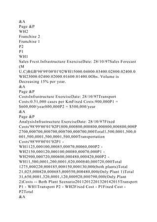
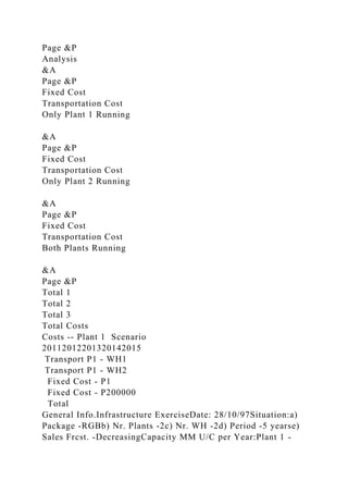
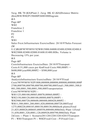
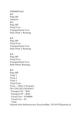
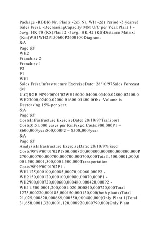
MGMT 511
Location Problem
George Heller was so successful in his previous assignment that
he was promoted to the coveted position of Infrastructure
Manager on the Mergers and Acquisitions Team.
Again Agame has recently acquired a competitive company with
a plant and a warehouse in a nearby city. Management has
decided to keep the additional warehouse. However, they are
unsure if they need to keep the additional manufacturing plant.
All products can be manufactured in either plant and shipped
from either warehouse. Each plant and each warehouse has
sufficient capacity to meet the total forecasted demand
individually.
Prepare a report for management with your recommendation.
Three possible choices exist. 1) Close the Competitor plant and
satisfy all demand from the Again Agame plant; 2) Close the
Again Agame plant and satisfy all demand from the Competitor
plant; 3)Keep both plants open.
Your recommendation should include a solution for each of the
five years in question. Include your calculations and
spreadsheets in support of your recommendations.
Sales Forecast (cases)
2011
2012
2013
2014
2015
Competitor Warehouse (WH1)
15,000,000
20,000,000
26,000,000
34,000,000
44,000,000
Again Agame Warehouse (WH2)
6,000,000
7,000,000
10,000,000
15,000,000
21,000,000
Fixed Costs
2011
2012
2013
2014
2015
Competitor Plant (P1)
900,000
900,000
900,000
900,000
900,000
Again Agame Plant (P2)
800,000
800,000
800,000
800,000
800,000
Transportation Costs
$1.00 / 1,000 cases / mile
4
Costs -- Both Plant Scenario
20112012201320142015
Transport P1 - WH1
Transport P2 - WH2
Fixed Cost - P1
Fixed Cost - P2
Total
General Info.Infrastructure ExerciseDate: 28/10/97Situation:a)
Package -RGBb) Nr. Plants -2c) Nr. WH -2d) Period -5 yearse)
Sales Frcst. -DecreasingCapacity MM U/C per Year:Plant 1 -
5avg. HK 70 (KS)Plant 2 -3avg. HK 42 (KS)Distance Matrix:
(Km)WH1WH2P150600P2600100Diagram:
&A
Page &P
WH2
Franchise 2
Franchise 1
P2
P1
WH1
Sales Frcst.Infrastructure ExerciseDate: 28/10/97Sales Forecast
(M
U.C)RGB'98'99'00'01'02WH15000.04000.03400.02800.02400.0
WH23000.02400.02000.01600.01400.0Obs. Volume is
Decreasing 15% per year.
&A
Page &P
CostsInfrastructure ExerciseDate: 28/10/97Transport
Costs:0.51,000 cases per KmFixed Costs:900,000P1 =
$600,000/year800,000P2 = $500,000/year
&A
Page &P
AnalysisInfrastructure ExerciseDate: 28/10/97Fixed
Costs'98'99'00'01'02P1800,000800,000800,000800,000800,000P
2700,000700,000700,000700,000700,000Total1,500,0001,500,0
001,500,0001,500,0001,500,000Transportation
Costs'98'99'00'01'02P1 -
WH1125,000100,00085,00070,00060,000P2 -
WH2150,000120,000100,00080,00070,000P1 -
WH2900,000720,000600,000480,000420,000P2 -
WH11,500,0001,200,0001,020,000840,000720,000Total
1275,000220,000185,000150,000130,000(both plants)Total
21,025,000820,000685,000550,000480,000(Only Plant 1)Total
31,650,0001,320,0001,120,000920,000790,000(Only Plant
2)Costs -- Both Plant Scenario20112012201320142015Transport
P1 - WH1Transport P2 - WH2Fixed Cost - P1Fixed Cost -
P2Total
&A
Page &P
Analysis
&A
Page &P
Fixed Cost
Transportation Cost
Only Plant 1 Running
&A
Page &P
Fixed Cost
Transportation Cost
Only Plant 2 Running
&A
Page &P
Fixed Cost
Transportation Cost
Both Plants Running
&A
Page &P
Total 1
Total 2
Total 3
Total Costs
Costs -- Plant 1 Scenario
20112012201320142015
Transport P1 - WH1
Transport P1 - WH2
Fixed Cost - P1
Fixed Cost - P200000
Total
General Info.Infrastructure ExerciseDate: 28/10/97Situation:a)
Package -RGBb) Nr. Plants -2c) Nr. WH -2d) Period -5 yearse)
Sales Frcst. -DecreasingCapacity MM U/C per Year:Plant 1 -
5avg. HK 70 (KS)Plant 2 -3avg. HK 42 (KS)Distance Matrix:
(Km)WH1WH2P150600P2600100Diagram:
&A
Page &P
WH2
Franchise 2
Franchise 1
P2
P1
WH1
Sales Frcst.Infrastructure ExerciseDate: 28/10/97Sales Forecast
(M
U.C)RGB'98'99'00'01'02WH15000.04000.03400.02800.02400.0
WH23000.02400.02000.01600.01400.0Obs. Volume is
Decreasing 15% per year.
&A
Page &P
CostsInfrastructure ExerciseDate: 28/10/97Transport
Costs:0.51,000 cases per KmFixed Costs:900,000P1 =
$600,000/year800,000P2 = $500,000/year
&A
Page &P
AnalysisInfrastructure ExerciseDate: 28/10/97Fixed
Costs'98'99'00'01'02P1800,000800,000800,000800,000800,000P
2700,000700,000700,000700,000700,000Total1,500,0001,500,0
001,500,0001,500,0001,500,000Transportation
Costs'98'99'00'01'02P1 -
WH1125,000100,00085,00070,00060,000P2 -
WH2150,000120,000100,00080,00070,000P1 -
WH2900,000720,000600,000480,000420,000P2 -
WH11,500,0001,200,0001,020,000840,000720,000Total
1275,000220,000185,000150,000130,000(both plants)Total
21,025,000820,000685,000550,000480,000(Only Plant 1)Total
31,650,0001,320,0001,120,000920,000790,000(Only Plant
2)Costs -- Plant 1 Scenario20112012201320142015Transport
P1 - WH1Transport P1 - WH2Fixed Cost - P1Fixed Cost -
P200000Total
&A
Page &P
Analysis
&A
Page &P
Fixed Cost
Transportation Cost
Only Plant 1 Running
&A
Page &P
Fixed Cost
Transportation Cost
Only Plant 2 Running
&A
Page &P
Fixed Cost
Transportation Cost
Both Plants Running
&A
Page &P
Total 1
Total 2
Total 3
Total Costs
Costs -- Plant 2 Scenario
20112012201320142015
Transport P2 - WH1
Transport P2 - WH2
Fixed Cost - P100000
Fixed Cost - P2
Total
General Info.Infrastructure ExerciseDate: 28/10/97Situation:a)
Package -RGBb) Nr. Plants -2c) Nr. WH -2d) Period -5 yearse)
Sales Frcst. -DecreasingCapacity MM U/C per Year:Plant 1 -
5avg. HK 70 (KS)Plant 2 -3avg. HK 42 (KS)Distance Matrix:
(Km)WH1WH2P150600P2600100Diagram:
&A
Page &P
WH2
Franchise 2
Franchise 1
P2
P1
WH1
Sales Frcst.Infrastructure ExerciseDate: 28/10/97Sales Forecast
(M
U.C)RGB'98'99'00'01'02WH15000.04000.03400.02800.02400.0
WH23000.02400.02000.01600.01400.0Obs. Volume is
Decreasing 15% per year.
&A
Page &P
CostsInfrastructure ExerciseDate: 28/10/97Transport
Costs:0.51,000 cases per KmFixed Costs:900,000P1 =
$600,000/year800,000P2 = $500,000/year
&A
Page &P
AnalysisInfrastructure ExerciseDate: 28/10/97Fixed
Costs'98'99'00'01'02P1800,000800,000800,000800,000800,000P
2700,000700,000700,000700,000700,000Total1,500,0001,500,0
001,500,0001,500,0001,500,000Transportation
Costs'98'99'00'01'02P1 -
WH1125,000100,00085,00070,00060,000P2 -
WH2150,000120,000100,00080,00070,000P1 -
WH2900,000720,000600,000480,000420,000P2 -
WH11,500,0001,200,0001,020,000840,000720,000Total
1275,000220,000185,000150,000130,000(both plants)Total
21,025,000820,000685,000550,000480,000(Only Plant 1)Total
31,650,0001,320,0001,120,000920,000790,000(Only Plant
2)Costs -- Plant 2 Scenario20112012201320142015Transport P2
- WH1Transport P2 - WH2Fixed Cost - P100000Fixed Cost -
P2Total
&A
Page &P
Analysis
&A
Page &P
Fixed Cost
Transportation Cost
Only Plant 1 Running
&A
Page &P
Fixed Cost
Transportation Cost
Only Plant 2 Running
&A
Page &P
Fixed Cost
Transportation Cost
Both Plants Running
&A
Page &P
Total 1
Total 2
Total 3
Total Costs
12. The U.S. Department of Transportation provides the number
of miles that residents of the 75 largest metropolitan areas
travel per day in a car. Suppose that for a simple random sample
of 50 Buffalo residents the mean is 22.5 miles a day and the
standard deviation is 8.4 miles a day, and for an independent
simple random sample of 40 Boston residents the mean is 18.6
miles a day and the standard deviation is 7.4 miles a day.
a) What is the point estimate of the difference between the mean
number of miles that Buffalo residents travel per day and the
mean number of miles that Boston residents travel per day?
b) What is the 95% confidence interval for the difference
between the two population means?
c) Do these cities have the same population means? State the
hypothesis and conclude using alpha = .05
22. A sample of 10 international telephone calls provided Sprint
and WorldCom calling rates per minute for calls from the
United States.
Country
Sprint
WorldCom
Australia
.46
.26
Belgium
.69
.40
Brazil
.92
.53
Colombia
.55
.53
Denmark
.50
.26
France
.46
.26
Germany
.46
.26
Hong Kong
.92
.40
Japan
.69
.40
United Kingdom
.46
.26
Provide a 95% confidence interval estimate of the difference
between the two population means.
34.New York City, Boston, and Silicon Valley of California are
among the areas with the highest technology salaries in the
United States. The following sample data show individual
annual salaries reported in thousands of dollars.
New York City
Boston
Silicon Valley
82
85
82
79
80
91
72
74
94
89
78
88
79
75
85
85
80
86
74
Use α = .05 and test for a significance difference among the
population mean annual technology salaries for these locations.
What is the p-value? What is your conclusion? If a difference
exists, which location appears to have the highest mean
technology salary?
2

MGMT 511Location ProblemGeorge Heller was so successful in.docx

  • 1.
    MGMT 511 Location Problem GeorgeHeller was so successful in his previous assignment that he was promoted to the coveted position of Infrastructure Manager on the Mergers and Acquisitions Team. Again Agame has recently acquired a competitive company with a plant and a warehouse in a nearby city. Management has decided to keep the additional warehouse. However, they are unsure if they need to keep the additional manufacturing plant. All products can be manufactured in either plant and shipped from either warehouse. Each plant and each warehouse has sufficient capacity to meet the total forecasted demand individually. Prepare a report for management with your recommendation. Three possible choices exist. 1) Close the Competitor plant and satisfy all demand from the Again Agame plant; 2) Close the Again Agame plant and satisfy all demand from the Competitor plant; 3)Keep both plants open. Your recommendation should include a solution for each of the five years in question. Include your calculations and spreadsheets in support of your recommendations. Sales Forecast (cases) 2011 2012 2013 2014 2015
  • 2.
    Competitor Warehouse (WH1) 15,000,000 20,000,000 26,000,000 34,000,000 44,000,000 AgainAgame Warehouse (WH2) 6,000,000 7,000,000 10,000,000 15,000,000 21,000,000 Fixed Costs 2011 2012 2013 2014 2015 Competitor Plant (P1) 900,000 900,000 900,000 900,000 900,000 Again Agame Plant (P2) 800,000 800,000 800,000 800,000
  • 3.
  • 4.
    4 Costs -- BothPlant Scenario 20112012201320142015 Transport P1 - WH1 Transport P2 - WH2 Fixed Cost - P1 Fixed Cost - P2 Total General Info.Infrastructure ExerciseDate: 28/10/97Situation:a) Package -RGBb) Nr. Plants -2c) Nr. WH -2d) Period -5 yearse) Sales Frcst. -DecreasingCapacity MM U/C per Year:Plant 1 - 5avg. HK 70 (KS)Plant 2 -3avg. HK 42 (KS)Distance Matrix: (Km)WH1WH2P150600P2600100Diagram:
  • 5.
    &A Page &P WH2 Franchise 2 Franchise1 P2 P1 WH1 Sales Frcst.Infrastructure ExerciseDate: 28/10/97Sales Forecast (M U.C)RGB'98'99'00'01'02WH15000.04000.03400.02800.02400.0 WH23000.02400.02000.01600.01400.0Obs. Volume is Decreasing 15% per year. &A Page &P CostsInfrastructure ExerciseDate: 28/10/97Transport Costs:0.51,000 cases per KmFixed Costs:900,000P1 = $600,000/year800,000P2 = $500,000/year &A Page &P AnalysisInfrastructure ExerciseDate: 28/10/97Fixed Costs'98'99'00'01'02P1800,000800,000800,000800,000800,000P 2700,000700,000700,000700,000700,000Total1,500,0001,500,0 001,500,0001,500,0001,500,000Transportation Costs'98'99'00'01'02P1 - WH1125,000100,00085,00070,00060,000P2 - WH2150,000120,000100,00080,00070,000P1 - WH2900,000720,000600,000480,000420,000P2 - WH11,500,0001,200,0001,020,000840,000720,000Total 1275,000220,000185,000150,000130,000(both plants)Total 21,025,000820,000685,000550,000480,000(Only Plant 1)Total 31,650,0001,320,0001,120,000920,000790,000(Only Plant 2)Costs -- Both Plant Scenario20112012201320142015Transport P1 - WH1Transport P2 - WH2Fixed Cost - P1Fixed Cost - P2Total &A
  • 6.
    Page &P Analysis &A Page &P FixedCost Transportation Cost Only Plant 1 Running &A Page &P Fixed Cost Transportation Cost Only Plant 2 Running &A Page &P Fixed Cost Transportation Cost Both Plants Running &A Page &P Total 1 Total 2 Total 3 Total Costs Costs -- Plant 1 Scenario 20112012201320142015 Transport P1 - WH1 Transport P1 - WH2 Fixed Cost - P1 Fixed Cost - P200000 Total General Info.Infrastructure ExerciseDate: 28/10/97Situation:a) Package -RGBb) Nr. Plants -2c) Nr. WH -2d) Period -5 yearse) Sales Frcst. -DecreasingCapacity MM U/C per Year:Plant 1 -
  • 7.
    5avg. HK 70(KS)Plant 2 -3avg. HK 42 (KS)Distance Matrix: (Km)WH1WH2P150600P2600100Diagram: &A Page &P WH2 Franchise 2 Franchise 1 P2 P1 WH1 Sales Frcst.Infrastructure ExerciseDate: 28/10/97Sales Forecast (M U.C)RGB'98'99'00'01'02WH15000.04000.03400.02800.02400.0 WH23000.02400.02000.01600.01400.0Obs. Volume is Decreasing 15% per year. &A Page &P CostsInfrastructure ExerciseDate: 28/10/97Transport Costs:0.51,000 cases per KmFixed Costs:900,000P1 = $600,000/year800,000P2 = $500,000/year &A Page &P AnalysisInfrastructure ExerciseDate: 28/10/97Fixed Costs'98'99'00'01'02P1800,000800,000800,000800,000800,000P 2700,000700,000700,000700,000700,000Total1,500,0001,500,0 001,500,0001,500,0001,500,000Transportation Costs'98'99'00'01'02P1 - WH1125,000100,00085,00070,00060,000P2 - WH2150,000120,000100,00080,00070,000P1 - WH2900,000720,000600,000480,000420,000P2 - WH11,500,0001,200,0001,020,000840,000720,000Total 1275,000220,000185,000150,000130,000(both plants)Total 21,025,000820,000685,000550,000480,000(Only Plant 1)Total 31,650,0001,320,0001,120,000920,000790,000(Only Plant 2)Costs -- Plant 1 Scenario20112012201320142015Transport P1 - WH1Transport P1 - WH2Fixed Cost - P1Fixed Cost -
  • 8.
    P200000Total &A Page &P Analysis &A Page &P FixedCost Transportation Cost Only Plant 1 Running &A Page &P Fixed Cost Transportation Cost Only Plant 2 Running &A Page &P Fixed Cost Transportation Cost Both Plants Running &A Page &P Total 1 Total 2 Total 3 Total Costs Costs -- Plant 2 Scenario 20112012201320142015 Transport P2 - WH1 Transport P2 - WH2 Fixed Cost - P100000 Fixed Cost - P2 Total General Info.Infrastructure ExerciseDate: 28/10/97Situation:a)
  • 9.
    Package -RGBb) Nr.Plants -2c) Nr. WH -2d) Period -5 yearse) Sales Frcst. -DecreasingCapacity MM U/C per Year:Plant 1 - 5avg. HK 70 (KS)Plant 2 -3avg. HK 42 (KS)Distance Matrix: (Km)WH1WH2P150600P2600100Diagram: &A Page &P WH2 Franchise 2 Franchise 1 P2 P1 WH1 Sales Frcst.Infrastructure ExerciseDate: 28/10/97Sales Forecast (M U.C)RGB'98'99'00'01'02WH15000.04000.03400.02800.02400.0 WH23000.02400.02000.01600.01400.0Obs. Volume is Decreasing 15% per year. &A Page &P CostsInfrastructure ExerciseDate: 28/10/97Transport Costs:0.51,000 cases per KmFixed Costs:900,000P1 = $600,000/year800,000P2 = $500,000/year &A Page &P AnalysisInfrastructure ExerciseDate: 28/10/97Fixed Costs'98'99'00'01'02P1800,000800,000800,000800,000800,000P 2700,000700,000700,000700,000700,000Total1,500,0001,500,0 001,500,0001,500,0001,500,000Transportation Costs'98'99'00'01'02P1 - WH1125,000100,00085,00070,00060,000P2 - WH2150,000120,000100,00080,00070,000P1 - WH2900,000720,000600,000480,000420,000P2 - WH11,500,0001,200,0001,020,000840,000720,000Total 1275,000220,000185,000150,000130,000(both plants)Total 21,025,000820,000685,000550,000480,000(Only Plant 1)Total 31,650,0001,320,0001,120,000920,000790,000(Only Plant
  • 10.
    2)Costs -- Plant2 Scenario20112012201320142015Transport P2 - WH1Transport P2 - WH2Fixed Cost - P100000Fixed Cost - P2Total &A Page &P Analysis &A Page &P Fixed Cost Transportation Cost Only Plant 1 Running &A Page &P Fixed Cost Transportation Cost Only Plant 2 Running &A Page &P Fixed Cost Transportation Cost Both Plants Running &A Page &P Total 1 Total 2 Total 3 Total Costs 12. The U.S. Department of Transportation provides the number of miles that residents of the 75 largest metropolitan areas travel per day in a car. Suppose that for a simple random sample of 50 Buffalo residents the mean is 22.5 miles a day and the standard deviation is 8.4 miles a day, and for an independent
  • 11.
    simple random sampleof 40 Boston residents the mean is 18.6 miles a day and the standard deviation is 7.4 miles a day. a) What is the point estimate of the difference between the mean number of miles that Buffalo residents travel per day and the mean number of miles that Boston residents travel per day? b) What is the 95% confidence interval for the difference between the two population means? c) Do these cities have the same population means? State the hypothesis and conclude using alpha = .05 22. A sample of 10 international telephone calls provided Sprint and WorldCom calling rates per minute for calls from the United States. Country Sprint WorldCom Australia .46 .26 Belgium .69 .40 Brazil .92 .53 Colombia .55 .53 Denmark .50 .26 France .46 .26 Germany .46
  • 12.
    .26 Hong Kong .92 .40 Japan .69 .40 United Kingdom .46 .26 Providea 95% confidence interval estimate of the difference between the two population means. 34.New York City, Boston, and Silicon Valley of California are among the areas with the highest technology salaries in the United States. The following sample data show individual annual salaries reported in thousands of dollars. New York City Boston Silicon Valley 82 85 82 79 80 91 72 74 94 89 78 88 79 75 85
  • 13.
    85 80 86 74 Use α =.05 and test for a significance difference among the population mean annual technology salaries for these locations. What is the p-value? What is your conclusion? If a difference exists, which location appears to have the highest mean technology salary? 2