Downloaded 128 times


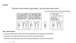


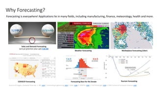


The document presents a comprehensive overview of using machine learning for forecasting, emphasizing the significance of time series analysis, feature engineering, and various machine learning techniques. It discusses best practices for data governance, forecasting accuracy determinants, types of forecasts, and the importance of model evaluation and deployment strategies. Additionally, it includes a tutorial on deep learning with TensorFlow and highlights the applications of forecasting across various industries.