This paper presents a geometric approach to the coordinatization of a measured space called the Map Maker’s algorithm. The measured space is defined by a distance matrix for sites which are reordered and mapped to points in a two-dimensional Euclidean space. The algorithm is tested on distance matrices created from 2D random point sets and the resulting coordinatizations compared with the original point sets for confirmation. Tolerance levels are set to deal with the cumulative numerical errors in the processing of the algorithm. The final point sets are found to be the same apart from translations, reflections and rotations as expected. The algorithm also serves as a method for projecting higher dimensional data to 2D.

1. International Journal of Computer Graphics & Animation (IJCGA) Vol.3, No.2, April 2013
DOI : 10.5121/ijcga.2013.3202 11
MAP MAKING FROM TABLES
John R Rankin
Department of Computer Science and Computer Engineering,
La Trobe University, Australia
j.rankin@latrobe.edu.au
ABSTRACT
This paper presents a geometric approach to the coordinatization of a measured space called the Map
Maker’s algorithm. The measured space is defined by a distance matrix for sites which are reordered and
mapped to points in a two-dimensional Euclidean space. The algorithm is tested on distance matrices
created from 2D random point sets and the resulting coordinatizations compared with the original point
sets for confirmation. Tolerance levels are set to deal with the cumulative numerical errors in the
processing of the algorithm. The final point sets are found to be the same apart from translations,
reflections and rotations as expected. The algorithm also serves as a method for projecting higher
dimensional data to 2D.
KEYWORDS
N-dimensional Space, Projections, Distance Matrices, Coordinatization
1.INTRODUCTION
The most primitive things that we can know of spaces are specific sites in those spaces and the
distances between them along given paths. This type of information is as old as history where
mankind recorded the names of cities or other localities and the approximate travel distances or
travel times between these sites. When maps were first drawn the sites needed to be located on a
flat 2D velum, parchment or sheet of paper. In cartesian geometry introduced much later in the
17th century AD [1] every position on the flat sheet has determinable intrinsic coordinates
labelled as (x,y) defined relative to a selected origin and a selected pair of perpendicular axial
directions in that plane.
A measured space is defined as a set of N sites Si labelled by index i = 1 to N together with their
distance matrix dij where dij is the distance between site i and site j for i and j ranging from 1 to
N with that distance measured along a prescribed path which should be the shortest available
connection between sites i and j. The archetypal case is where the Si are the names of N cities in a
particular country or district and dij are the recorded shortest distances between these cities by
using the road system of that country or district. This information can be presented in tabular
form. The information in tabular form is called a spatial description. Humans respond better to
pictures than to tables so the following question then arises. Given this tabular information only is
it possible to create a pictorial map representing this space showing the sites in relative positions
such that the actual distances between the sites is a scaled up version of the distances between the
points on the flat 2D map? This form of representing the space is called the pictorial map or the
geometric form and such maps have been drawn from time immemorial. It is known that one can
easily convert from the geometric or pictorial form to the tabular form. To do so one simply takes
all required measurements off the map to fill in the distance matrix of the tabular form. But is it

2. International Journal of Computer Graphics & Animation (IJCGA) Vol.3, No.2, April 2013
12
possible to create the geometric form from the tabular form alone? This paper provides an
algorithm for doing this conversion called the Map Maker’s algorithm and also shows how the
algorithm will fail for general spatial descriptions. The process of conversion of higher
dimensional data to 2D data for viewing has been extensively researched [see eg 2-12] but the
simple approach described here has not been presented before.
2.REORDERING THE SITES
The order of the sites for a measured space is unimportant and not significant for the measured
space itself. This is particularly obvious in the pictorial map view where there is clearly no
intrinsic linear ordering of the sites from the pictorial map view. Therefore the ordering of the
sites that appears in the descriptive form is not significant and any arbitrarily chosen ordering can
be used. In the case of a distance matrix for cities the sites may be for example ordered
alphabetically by the name of the city. Alternatively the cities may be ordered by population size
or some other non-spatial criterion such as road usage frequencies or recency of road works.
Sometimes a reordering can assist the algorithm or reduce numerical errors in the computation of
coordinates. Since errors accumulate we may choose to put the most frequently travelled paths
earlier in the algorithm rather than later so that the best accuracy applies to the most useful
connections between sites or alternatively reorder the sites from furthest separation to closest
separation to get better coordinatization accuracy on furthest distances and therefore also on the
coordinatizion for sites of smaller separation distances since they will have less absolute error for
the same relative error. The reordering is represented by a one-dimensional array R[i] so that in
place of the original ordering of the sites 1, 2, 3, ... N we have the new ordering denoted R[1],
R[2], R[3], ... R[N].
This paper proposes two site reordering methods which are based on net connection distances as
follows. For each site Si, compute the sum of the distances from that site to all other sites and
denote this as Di. The site with the smallest/largest value of Di is the most/least “connected” of
all the sites and it is chosen as the first site in the reordering i.e. R[1]. For site R[2] we select the
site with the second smallest/largest value of Di, for the site R[3] we select the site with the third
smallest/largest value of Di and so forth. It is conjectured that the second of these reorderings will
reduce the absolute numerical errors in applying the algorithm. This second reordering will
therefore be assumed in the following algorithm.
3.GEOMETRIC COORDINATIZATION
The origin of the 2D cartesian space can be selected arbitrarily. Therefore set the first (reordered)
site R[1] as located at the origin:
P1 = (0,0)
The direction of the x-axis of the 2D cartesian space can be selected arbitrarily. Therefore set the
line from site R[1] to site R[2], i.e. from P1 to P2 as the x-axis direction. Therefore to maintain
distance scales
P2 = (d12,0)
This effectively sets P2 as due East of P1 which may not be geographically correct if we are
dealing with localities on the surface of the Earth. However the choice is available to us since we
are allowed to turn the map around by any desired angle.

3. International Journal of Computer Graphics & Animation (IJCGA) Vol.3, No.2, April 2013
13
Now consider 2D coordinates for the point P3 corresponding to site R[3]. Figure 1 shows how
this is done. Points P1, P2 and P3 form a triangle whose sides are known. We need to determine
the angle α at P1 in order to get the coordinates (x,y) of P3. In the process of making the
coordinates of P3 we introduce the point Q which is such that P1P2 and QP3 are perpendicular
lines. This means that QP3 is pointing in the y-axis direction as shown in Figure 1. This
effectively sets P3 as to the North of P1 and P2 which may not be geographically correct if we are
dealing with localities on the surface of the Earth. However the choice is available to us since we
are allowed to turn the map upside-down if desired.
From the Law of Cosines and Figure 1 we deduce that
cos α = (d − d − d )/(2d d )
From this we compute the coordinates of P3 as:
x = d cos α
y = d 1 − cos α
To find the coordinates for P4 corresponding to site [4] we use the same approach as for site R[3].
However now we have the choice of a positive or negative y value for P4:
P = (d cosα , d 1 − cos α )
P = (d cosα , −d 1 − cos α )
where α is the angle computed at P1 for the triangle P1P2P4 i.e.
cos α = (d − d − d )/(2d d )
To determine which of P4+ and P4- is the correct point we compute the distances from P3 to P4+
and P4- and select the point P4+ or P4- for which the distance is closer to the given value of d34.
This process for determining the coordinates of P4 is applied to form P5 and so forth up to PN.
When choosing between Pi+ and Pi- for i > 4 we could look for any differences between
Distance(Pi+,Pj) and dR[i]R[j] for all j where 2 < j < i and if any significant difference occurred
we would choose Pi = Pi- instead of Pi = Pi+. However this algorithm assumes that the distance
matrix data comes from a flat two-dimensional space so only Distance(Pi+,P3) will be compared
with dR[i]R[3]. So the algorithm will proceed on the assumption that the measured space is flat
and two-dimensional and then after the algorithm is finished generating the coordinates of all

4. International Journal of Computer Graphics & Animation (IJCGA) Vol.3, No.2, April 2013
14
points Pi for i = 1 to N we can run a test to compute the RMS error of the distances between all
pairs of points, Distance(Pi,Pj), compared with dR[i]R[j]. If there is a significant RMS error then
the given measured space can be declared to not be a flat two-dimensional Euclidean space.
4.MAP MAKER’S ALGORITHM
The implementation of this approach in any computer language is quite straight forward. The
pseudocode of the algorithm including reordering is listed below.
for i = 1 to N
sum[i] = 0
for j = 1 to N
sum[i] = sum[i] + d[i,j]
Sort(sum[],R[])
P[1].x = 0
P[1].y = 0
P[2].x = d[R[1],R[2])
P[2].y = 0
cosalpha = (Sq(d[R[2],R[3]]) - Sq(d[R[1],R[2]])- Sq(d[R[1],R[3]]))/2/d[R[1],R[2]]/d[R[1],R[3]]
P[3].x = d[R[1],R[3]]*cosalpha
P[3].y = d[R[1],R[3]]*SqRoot(1 - Sq(cosalpha))
for i = 4 to N
cosalpha = (Sq(d[R[2],R[i]]) - Sq(d[R[1],R[2]]) -
Sq(d[R[1],R[i]]))/2/d[R[1],R[2]]/d[R[1],R[i]]
P[i].x = d[R[1],R[i]]*cosalpha
P[i].y = d[R[1],R[i]]*SqRoot(1 - Sq(cosalpha))
if (Distance(P[i],P[3]) != d[R[i],R[3]])
P[i].y = -d[R[1],R[i]]*SqRoot(1 - Sq(cosalpha))
The output of this algorithm is then the set of 2D points P[i] for i = 1 to N and these are then
plotted on a 2D graph.
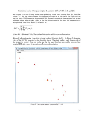
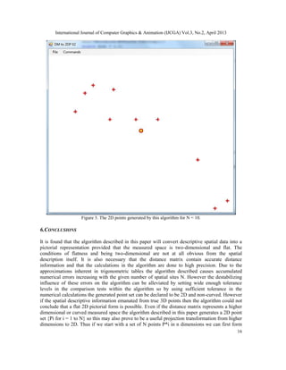
5.RESULTS
To test this algorithm several support programs and test data were created as described below.
Cases of N were chosen as 3, 4 and 10. Then using a program called Random 2D Points a set of
N random 2D points was created and stored in a file in 2DP format. The 2DP format is a simple
text file format where the first line contains only the number of points N that are stored in the file
and the following N lines of the file contain the point data with P[i].x and P[i].y space separated
on the ith line following the first line of the file. A program called View 2DP can input files of
this type and plot the data as points on the graphics screen. Another program called Make DM
reads in 2DP files and outputs the distance matrix as a DM file. The DM format is a simple text
file format where the first line contains only the number of points N and the following N lines of
the file contain the point distance data as d[i,1], d[i,2], d[i,3]... to d[i,N] space separated on the ith
line following the first line of the file. A program called DM to 2DP with the above algorithm
reads in a DM file as input and computes the point coordinates via the above Map Maker’s
algorithm and outputs them to a file of type 2DP. Subsequently we view the output 2DP file using
the View 2DP program again and then compare this second 2DP data visually with the view of

5. International Journal of Computer Graphics & Animation (IJCGA) Vol.3, No.2, April 2013
15
the original 2DP data. If they are the same pictorially except for a rotation about P1, reflection
about P1P2 and any translation then the algorithm is deemed to be successful. The final test is to
use the Make DM program on the generated 2DP data and compare the data values of the second
distance matrix with the data values in the first distance matrix. To make the comparison we
computer the Root Mean Square (RMS) error as:
∑∑= =
−=
N
i
N
j
ijij ddRMS
1 1
2
)'(
where d’ij = Distance(Pi,Pj). The results of this testing will be presented elsewhere.
Figure 2 below shows the view of the original random 2D points for N = 10. Figure 3 shows the
view of the 2DP file generated by the algorithm above. (The circle markers mark the centroids of
the respective points.) One can easily see that the algorithm has successfully recovered the
original 2DP data except for a rotation, reflection and translation.
Figure 2. The original random 2D points for N = 10.

6. International Journal of Computer Graphics & Animation (IJCGA) Vol.3, No.2, April 2013
16
Figure 3. The 2D points generated by this algorithm for N = 10.
6.CONCLUSIONS
It is found that the algorithm described in this paper will convert descriptive spatial data into a
pictorial representation provided that the measured space is two-dimensional and flat. The
conditions of flatness and being two-dimensional are not at all obvious from the spatial
description itself. It is also necessary that the distance matrix contain accurate distance
information and that the calculations in the algorithm are done to high precision. Due to the
approximations inherent in trigonometric tables the algorithm described causes accumulated
numerical errors increasing with the given number of spatial sites N. However the destabilizing
influence of these errors on the algorithm can be alleviated by setting wide enough tolerance
levels in the comparison tests within the algorithm so by using sufficient tolerance in the
numerical calculations the generated point set can be declared to be 2D and non-curved. However
if the spatial descriptive information emanated from true 3D points then the algorithm could not
conclude that a flat 2D pictorial form is possible. Even if the distance matrix represents a higher
dimensional or curved measured space the algorithm described in this paper generates a 2D point
set {Pi for i = 1 to N} so this may also prove to be a useful projection transformation from higher
dimensions to 2D. Thus if we start with a set of N points P*i in n dimensions we can first form

7. International Journal of Computer Graphics & Animation (IJCGA) Vol.3, No.2, April 2013
17
the distance matrix from the n-dimensional points and then apply the Map Maker’s algorithm to
obtain the corresponding points Pi in two dimensions for plotting.
REFERENCES
[1] See “Cartesian coordinate system” in the online Wikipedia at url
http://en.wikipedia.org/wiki/Cartesian_coordinate_system
[2] Lee RTC et al, “A Triangulation Method for the Sequential Mapping of Points from N-Space to
Two-Space”, IEEE Transactions on Computers, March 1977, pp288-292.
[3] Yin H, “Nonlinear Dimensionality Reduction and Data Visualization: A Review”, International
Journal of Automation and Computing 04(3), July 2007, pp294-303.
[4] Sammon J W Jr, “A Nonlinear Mapping for Data Structure Analysis”, IEE Transaction on
Computers, Vol C-18, No. 5, May 1969, pp401-409.
[5] Shisko JF et al, “IGODS: An Important New Tool for Managing and Visualizing Spatial Data”,
OCEANS 2010, pp1-10.
[6] Li Q et al, “A Chunking Method for Euclidean Distance Matrix Calculation on Large Dataset Using
Multi-GPU”, IEEE Machine Learning and Applications (ICMLA) Dec 2010, pp 208-213.
[7] Hyo-Sung A, “Command Coordination In Multi-Agent Formation: A Distance Matrix Approach”,
IEEE Control Automation and Systems (ICCAS) 2010, pp 1592-1597.
[8] Srinkanthan S, “Accelerating the Euclidean Distance Matrix Computation Using GPUs”, IEEE
Electronics Computer Technology (ICECT) 2011, pp422-426.
[9] Del Bue A et al, “2D-3D Registration of Deformable Shapes with Manifold Projection”, 2009, pp
1061-1064.
[10] Drineas P et al, “Distance Matrix Reconstruction from Incomplete Distance Information for Sensor
Network Localization”, Sensor and Ad Hoc Communications and Networks 2006, pp 536-544.
[11] Ayhan S et al “Implementing Geospatially Enabled Aviation Web Services”, Integrated
Communications, Navigation and Surveillance (ICNS) 2008, pp1-8.
[12] Xiao Q et al,“Application of Visualization Technology in Spatial Data Mining”, Computing, Control
and Industrial Engineering (CCIE), 2010, pp153-157.