A First Course in Probability is a comprehensive textbook by Sheldon Ross, now in its eighth edition, covering fundamental concepts in probability theory. The book includes topics like combinatorial analysis, axioms of probability, random variables, and joint distributions, along with numerous exercises for practice. It is designed for students seeking to understand and apply probability concepts in various domains.

2. A FIRST COURSE IN PROBABILITY

3. This page intentionally left blank

4. A FIRST COURSE IN PROBABILITY
Eighth Edition
Sheldon Ross
University of Southern California
Upper Saddle River, New Jersey 07458

5. Library of Congress Cataloging-in-Publication Data
Ross, Sheldon M.
A first course in probability / Sheldon Ross. — 8th ed.
p. cm.
Includes bibliographical references and index.
ISBN-13: 978-0-13-603313-4
ISBN-10: 0-13-603313-X
1. Probabilities—Textbooks. I. Title.
QA273.R83 2010
519.2—dc22
2008033720
Editor in Chief, Mathematics and Statistics: Deirdre Lynch
Senior Project Editor: Rachel S. Reeve
Assistant Editor: Christina Lepre
Editorial Assistant: Dana Jones
Project Manager: Robert S. Merenoff
Associate Managing Editor: Bayani Mendoza de Leon
Senior Managing Editor: Linda Mihatov Behrens
Senior Operations Supervisor: Diane Peirano
Marketing Assistant: Kathleen DeChavez
Creative Director: Jayne Conte
Art Director/Designer: Bruce Kenselaar
AV Project Manager: Thomas Benfatti
Compositor: Integra Software Services Pvt. Ltd, Pondicherry, India
Cover Image Credit: Getty Images, Inc.
© 2010, 2006, 2002, 1998, 1994, 1988,
1984, 1976 by Pearson Education, Inc.,
Pearson Prentice Hall
Pearson Education, Inc.
Upper Saddle River, NJ 07458
All rights reserved. No part of this book may be reproduced, in any
form or by any means, without permission in writing from the publisher.
Pearson Prentice Hall™ is a trademark of Pearson Education, Inc.
Printed in the United States of America
10 9 8 7 6 5 4 3 2 1
ISBN-13: 978-0-13-603313-4
ISBN-10: 0-13-603313-X
Pearson Education, Ltd., London
Pearson Education Australia PTY. Limited, Sydney
Pearson Education Singapore, Pte. Ltd
Pearson Education North Asia Ltd, Hong Kong
Pearson Education Canada, Ltd., Toronto
Pearson Educación de Mexico, S.A. de C.V.
Pearson Education – Japan, Tokyo
Pearson Education Malaysia, Pte. Ltd
Pearson Education Upper Saddle River, New Jersey

6. For Rebecca

7. This page intentionally left blank

8. Contents
Preface xi
1 Combinatorial Analysis 1
1.1 Introduction . . . . . . . . . . . . . . . . . . . . . . . . . . . . . . . . . 1
1.2 The Basic Principle of Counting . . . . . . . . . . . . . . . . . . . . . . 1
1.3 Permutations . . . . . . . . . . . . . . . . . . . . . . . . . . . . . . . . . 3
1.4 Combinations . . . . . . . . . . . . . . . . . . . . . . . . . . . . . . . . 5
1.5 Multinomial Coefficients . . . . . . . . . . . . . . . . . . . . . . . . . . 9
1.6 The Number of Integer Solutions of Equations . . . . . . . . . . . . . 12
Summary . . . . . . . . . . . . . . . . . . . . . . . . . . . . . . . . . . . 15
Problems . . . . . . . . . . . . . . . . . . . . . . . . . . . . . . . . . . . 16
Theoretical Exercises . . . . . . . . . . . . . . . . . . . . . . . . . . . . 18
Self-Test Problems and Exercises . . . . . . . . . . . . . . . . . . . . . 20
2 Axioms of Probability 22
2.1 Introduction . . . . . . . . . . . . . . . . . . . . . . . . . . . . . . . . . 22
2.2 Sample Space and Events . . . . . . . . . . . . . . . . . . . . . . . . . . 22
2.3 Axioms of Probability . . . . . . . . . . . . . . . . . . . . . . . . . . . . 26
2.4 Some Simple Propositions . . . . . . . . . . . . . . . . . . . . . . . . . 29
2.5 Sample Spaces Having Equally Likely Outcomes . . . . . . . . . . . . 33
2.6 Probability as a Continuous Set Function . . . . . . . . . . . . . . . . . 44
2.7 Probability as a Measure of Belief . . . . . . . . . . . . . . . . . . . . . 48
Summary . . . . . . . . . . . . . . . . . . . . . . . . . . . . . . . . . . . 49
Problems . . . . . . . . . . . . . . . . . . . . . . . . . . . . . . . . . . . 50
Theoretical Exercises . . . . . . . . . . . . . . . . . . . . . . . . . . . . 54
Self-Test Problems and Exercises . . . . . . . . . . . . . . . . . . . . . 56
3 Conditional Probability and Independence 58
3.1 Introduction . . . . . . . . . . . . . . . . . . . . . . . . . . . . . . . . . 58
3.2 Conditional Probabilities . . . . . . . . . . . . . . . . . . . . . . . . . . 58
3.3 Bayes’s Formula . . . . . . . . . . . . . . . . . . . . . . . . . . . . . . . 65
3.4 Independent Events . . . . . . . . . . . . . . . . . . . . . . . . . . . . . 79
3.5 P(·|F) Is a Probability . . . . . . . . . . . . . . . . . . . . . . . . . . . . 93
Summary . . . . . . . . . . . . . . . . . . . . . . . . . . . . . . . . . . . 101
Problems . . . . . . . . . . . . . . . . . . . . . . . . . . . . . . . . . . . 102
Theoretical Exercises . . . . . . . . . . . . . . . . . . . . . . . . . . . . 110
Self-Test Problems and Exercises . . . . . . . . . . . . . . . . . . . . . 114
4 Random Variables 117
4.1 Random Variables . . . . . . . . . . . . . . . . . . . . . . . . . . . . . . 117
4.2 Discrete Random Variables . . . . . . . . . . . . . . . . . . . . . . . . 123
4.3 Expected Value . . . . . . . . . . . . . . . . . . . . . . . . . . . . . . . 125
4.4 Expectation of a Function of a Random Variable . . . . . . . . . . . . 128
4.5 Variance . . . . . . . . . . . . . . . . . . . . . . . . . . . . . . . . . . . 132
4.6 The Bernoulli and Binomial Random Variables . . . . . . . . . . . . . 134
4.6.1 Properties of Binomial Random Variables . . . . . . . . . . . . 139
4.6.2 Computing the Binomial Distribution Function . . . . . . . . . 142
vii

9. viii Contents
4.7 The Poisson Random Variable . . . . . . . . . . . . . . . . . . . . . . . 143
4.7.1 Computing the Poisson Distribution Function . . . . . . . . . . 154
4.8 Other Discrete Probability Distributions . . . . . . . . . . . . . . . . . 155
4.8.1 The Geometric Random Variable . . . . . . . . . . . . . . . . . 155
4.8.2 The Negative Binomial Random Variable . . . . . . . . . . . . 157
4.8.3 The Hypergeometric Random Variable . . . . . . . . . . . . . 160
4.8.4 The Zeta (or Zipf) Distribution . . . . . . . . . . . . . . . . . . 163
4.9 Expected Value of Sums of Random Variables . . . . . . . . . . . . . 164
4.10 Properties of the Cumulative Distribution Function . . . . . . . . . . . 168
Summary . . . . . . . . . . . . . . . . . . . . . . . . . . . . . . . . . . . 170
Problems . . . . . . . . . . . . . . . . . . . . . . . . . . . . . . . . . . . 172
Theoretical Exercises . . . . . . . . . . . . . . . . . . . . . . . . . . . . 179
Self-Test Problems and Exercises . . . . . . . . . . . . . . . . . . . . . 183
5 Continuous Random Variables 186
5.1 Introduction . . . . . . . . . . . . . . . . . . . . . . . . . . . . . . . . . 186
5.2 Expectation and Variance of Continuous Random Variables . . . . . 190
5.3 The Uniform Random Variable . . . . . . . . . . . . . . . . . . . . . . 194
5.4 Normal Random Variables . . . . . . . . . . . . . . . . . . . . . . . . . 198
5.4.1 The Normal Approximation to the Binomial Distribution . . . 204
5.5 Exponential Random Variables . . . . . . . . . . . . . . . . . . . . . . 208
5.5.1 Hazard Rate Functions . . . . . . . . . . . . . . . . . . . . . . . 212
5.6 Other Continuous Distributions . . . . . . . . . . . . . . . . . . . . . . 215
5.6.1 The Gamma Distribution . . . . . . . . . . . . . . . . . . . . . 215
5.6.2 The Weibull Distribution . . . . . . . . . . . . . . . . . . . . . 216
5.6.3 The Cauchy Distribution . . . . . . . . . . . . . . . . . . . . . . 217
5.6.4 The Beta Distribution . . . . . . . . . . . . . . . . . . . . . . . 218
5.7 The Distribution of a Function of a Random Variable . . . . . . . . . 219
Summary . . . . . . . . . . . . . . . . . . . . . . . . . . . . . . . . . . . 222
Problems . . . . . . . . . . . . . . . . . . . . . . . . . . . . . . . . . . . 224
Theoretical Exercises . . . . . . . . . . . . . . . . . . . . . . . . . . . . 227
Self-Test Problems and Exercises . . . . . . . . . . . . . . . . . . . . . 229
6 Jointly Distributed Random Variables 232
6.1 Joint Distribution Functions . . . . . . . . . . . . . . . . . . . . . . . . 232
6.2 Independent Random Variables . . . . . . . . . . . . . . . . . . . . . . 240
6.3 Sums of Independent Random Variables . . . . . . . . . . . . . . . . . 252
6.3.1 Identically Distributed Uniform Random Variables . . . . . . 252
6.3.2 Gamma Random Variables . . . . . . . . . . . . . . . . . . . . 254
6.3.3 Normal Random Variables . . . . . . . . . . . . . . . . . . . . 256
6.3.4 Poisson and Binomial Random Variables . . . . . . . . . . . . 259
6.3.5 Geometric Random Variables . . . . . . . . . . . . . . . . . . . 260
6.4 Conditional Distributions: Discrete Case . . . . . . . . . . . . . . . . . 263
6.5 Conditional Distributions: Continuous Case . . . . . . . . . . . . . . . 266
6.6 Order Statistics . . . . . . . . . . . . . . . . . . . . . . . . . . . . . . . 270
6.7 Joint Probability Distribution of Functions of Random Variables . . . 274
6.8 Exchangeable Random Variables . . . . . . . . . . . . . . . . . . . . . 282
Summary . . . . . . . . . . . . . . . . . . . . . . . . . . . . . . . . . . . 285
Problems . . . . . . . . . . . . . . . . . . . . . . . . . . . . . . . . . . . 287
Theoretical Exercises . . . . . . . . . . . . . . . . . . . . . . . . . . . . 291
Self-Test Problems and Exercises . . . . . . . . . . . . . . . . . . . . . 293

10. Contents ix
7 Properties of Expectation 297
7.1 Introduction . . . . . . . . . . . . . . . . . . . . . . . . . . . . . . . . . 297
7.2 Expectation of Sums of Random Variables . . . . . . . . . . . . . . . . 298
7.2.1 Obtaining Bounds from Expectations
via the Probabilistic Method . . . . . . . . . . . . . . . . . . . . 311
7.2.2 The Maximum–Minimums Identity . . . . . . . . . . . . . . . . 313
7.3 Moments of the Number of Events that Occur . . . . . . . . . . . . . . 315
7.4 Covariance, Variance of Sums, and Correlations . . . . . . . . . . . . . 322
7.5 Conditional Expectation . . . . . . . . . . . . . . . . . . . . . . . . . . 331
7.5.1 Definitions . . . . . . . . . . . . . . . . . . . . . . . . . . . . . . 331
7.5.2 Computing Expectations by Conditioning . . . . . . . . . . . . 333
7.5.3 Computing Probabilities by Conditioning . . . . . . . . . . . . 344
7.5.4 Conditional Variance . . . . . . . . . . . . . . . . . . . . . . . . 347
7.6 Conditional Expectation and Prediction . . . . . . . . . . . . . . . . . 349
7.7 Moment Generating Functions . . . . . . . . . . . . . . . . . . . . . . . 354
7.7.1 Joint Moment Generating Functions . . . . . . . . . . . . . . . 363
7.8 Additional Properties of Normal Random Variables . . . . . . . . . . 365
7.8.1 The Multivariate Normal Distribution . . . . . . . . . . . . . . 365
7.8.2 The Joint Distribution of the Sample Mean
and Sample Variance . . . . . . . . . . . . . . . . . . . . . . . . 367
7.9 General Definition of Expectation . . . . . . . . . . . . . . . . . . . . . 369
Summary . . . . . . . . . . . . . . . . . . . . . . . . . . . . . . . . . . . 370
Problems . . . . . . . . . . . . . . . . . . . . . . . . . . . . . . . . . . . 373
Theoretical Exercises . . . . . . . . . . . . . . . . . . . . . . . . . . . . 380
Self-Test Problems and Exercises . . . . . . . . . . . . . . . . . . . . . 384
8 Limit Theorems 388
8.1 Introduction . . . . . . . . . . . . . . . . . . . . . . . . . . . . . . . . . 388
8.2 Chebyshev’s Inequality and the Weak Law of Large
Numbers . . . . . . . . . . . . . . . . . . . . . . . . . . . . . . . . . . . 388
8.3 The Central Limit Theorem . . . . . . . . . . . . . . . . . . . . . . . . 391
8.4 The Strong Law of Large Numbers . . . . . . . . . . . . . . . . . . . . 400
8.5 Other Inequalities . . . . . . . . . . . . . . . . . . . . . . . . . . . . . . 403
8.6 Bounding the Error Probability When Approximating a Sum of
Independent Bernoulli Random Variables by a Poisson
Random Variable . . . . . . . . . . . . . . . . . . . . . . . . . . . . . . 410
Summary . . . . . . . . . . . . . . . . . . . . . . . . . . . . . . . . . . . 412
Problems . . . . . . . . . . . . . . . . . . . . . . . . . . . . . . . . . . . 412
Theoretical Exercises . . . . . . . . . . . . . . . . . . . . . . . . . . . . 414
Self-Test Problems and Exercises . . . . . . . . . . . . . . . . . . . . . 415
9 Additional Topics in Probability 417
9.1 The Poisson Process . . . . . . . . . . . . . . . . . . . . . . . . . . . . . 417
9.2 Markov Chains . . . . . . . . . . . . . . . . . . . . . . . . . . . . . . . . 419
9.3 Surprise, Uncertainty, and Entropy . . . . . . . . . . . . . . . . . . . . 425
9.4 Coding Theory and Entropy . . . . . . . . . . . . . . . . . . . . . . . . 428
Summary . . . . . . . . . . . . . . . . . . . . . . . . . . . . . . . . . . . 434
Problems and Theoretical Exercises . . . . . . . . . . . . . . . . . . . . 435
Self-Test Problems and Exercises . . . . . . . . . . . . . . . . . . . . . 436
References . . . . . . . . . . . . . . . . . . . . . . . . . . . . . . . . . . 436

11. x Contents
10 Simulation 438
10.1 Introduction . . . . . . . . . . . . . . . . . . . . . . . . . . . . . . . . . 438
10.2 General Techniques for Simulating Continuous Random Variables . . 440
10.2.1 The Inverse Transformation Method . . . . . . . . . . . . . . . 441
10.2.2 The Rejection Method . . . . . . . . . . . . . . . . . . . . . . . 442
10.3 Simulating from Discrete Distributions . . . . . . . . . . . . . . . . . . 447
10.4 Variance Reduction Techniques . . . . . . . . . . . . . . . . . . . . . . 449
10.4.1 Use of Antithetic Variables . . . . . . . . . . . . . . . . . . . . 450
10.4.2 Variance Reduction by Conditioning . . . . . . . . . . . . . . . 451
10.4.3 Control Variates . . . . . . . . . . . . . . . . . . . . . . . . . . 452
Summary . . . . . . . . . . . . . . . . . . . . . . . . . . . . . . . . . . . 453
Problems . . . . . . . . . . . . . . . . . . . . . . . . . . . . . . . . . . . 453
Self-Test Problems and Exercises . . . . . . . . . . . . . . . . . . . . . 455
Reference . . . . . . . . . . . . . . . . . . . . . . . . . . . . . . . . . . 455
Answers to Selected Problems 457
Solutions to Self-Test Problems and Exercises 461
Index 521

12. Preface
“We see that the theory of probability is at bottom only common sense reduced
to calculation; it makes us appreciate with exactitude what reasonable minds feel
by a sort of instinct, often without being able to account for it. ... It is remarkable
that this science, which originated in the consideration of games of chance, should
have become the most important object of human knowledge. ... The most important
questions of life are, for the most part, really only problems of probability.” So said
the famous French mathematician and astronomer (the “Newton of France”) Pierre-
Simon, Marquis de Laplace. Although many people feel that the famous marquis,
who was also one of the great contributors to the development of probability, might
have exaggerated somewhat, it is nevertheless true that probability theory has become
a tool of fundamental importance to nearly all scientists, engineers, medical practi-
tioners, jurists, and industrialists. In fact, the enlightened individual had learned to
ask not “Is it so?” but rather “What is the probability that it is so?”
This book is intended as an elementary introduction to the theory of probability
for students in mathematics, statistics, engineering, and the sciences (including com-
puter science, biology, the social sciences, and management science) who possess the
prerequisite knowledge of elementary calculus. It attempts to present not only the
mathematics of probability theory, but also, through numerous examples, the many
diverse possible applications of this subject.
Chapter 1 presents the basic principles of combinatorial analysis, which are most
useful in computing probabilities.
Chapter 2 handles the axioms of probability theory and shows how they can be
applied to compute various probabilities of interest.
Chapter 3 deals with the extremely important subjects of conditional probability
and independence of events. By a series of examples, we illustrate how conditional
probabilities come into play not only when some partial information is available,
but also as a tool to enable us to compute probabilities more easily, even when
no partial information is present. This extremely important technique of obtaining
probabilities by “conditioning” reappears in Chapter 7, where we use it to obtain
expectations.
The concept of random variables is introduced in Chapters 4, 5, and 6. Discrete
random variables are dealt with in Chapter 4, continuous random variables in
Chapter 5, and jointly distributed random variables in Chapter 6. The important con-
cepts of the expected value and the variance of a random variable are introduced in
Chapters 4 and 5, and these quantities are then determined for many of the common
types of random variables.
Additional properties of the expected value are considered in Chapter 7. Many
examples illustrating the usefulness of the result that the expected value of a sum of
random variables is equal to the sum of their expected values are presented. Sections
on conditional expectation, including its use in prediction, and on moment-generating
functions are contained in this chapter. In addition, the final section introduces the
multivariate normal distribution and presents a simple proof concerning the joint
distribution of the sample mean and sample variance of a sample from a normal
distribution.
xi

13. xii Preface
Chapter 8 presents the major theoretical results of probability theory. In partic-
ular, we prove the strong law of large numbers and the central limit theorem. Our
proof of the strong law is a relatively simple one which assumes that the random vari-
ables have a finite fourth moment, and our proof of the central limit theorem assumes
Levy’s continuity theorem. This chapter also presents such probability inequalities as
Markov’s inequality, Chebyshev’s inequality, and Chernoff bounds. The final section
of Chapter 8 gives a bound on the error involved when a probability concerning
a sum of independent Bernoulli random variables is approximated by the corre-
sponding probability of a Poisson random variable having the same expected
value.
Chapter 9 presents some additional topics, such as Markov chains, the Poisson pro-
cess, and an introduction to information and coding theory, and Chapter 10 considers
simulation.
As in the previous edition, three sets of exercises are given at the end of each
chapter. They are designated as Problems, Theoretical Exercises, and Self-Test Prob-
lems and Exercises. This last set of exercises, for which complete solutions appear in
Solutions to Self-Test Problems and Exercises, is designed to help students test their
comprehension and study for exams.
CHANGES IN THE NEW EDITION
The eighth edition continues the evolution and fine tuning of the text. It includes
new problems, exercises, and text material chosen both for its inherent interest and
for its use in building student intuition about probability. Illustrative of these goals
are Example 5d of Chapter 1 on knockout tournaments, and Examples 4k and 5i of
Chapter 7 on multiple player gambler’s ruin problems.
A key change in the current edition is that the important result that the expectation
of a sum of random variables is equal to the sum of the expectations is now first
presented in Chapter 4 (rather than Chapter 7 as in previous editions). A new and
elementary proof of this result when the sample space of the probability experiment
is finite is given in this chapter.
Another change is the expansion of Section 6.3, which deals with the sum of inde-
pendent random variables. Section 6.3.1 is a new section in which we derive the
distribution of the sum of independent and identically distributed uniform random
variables, and then use our results to show that the expected number of random num-
bers that needs to be added for their sum to exceed 1 is equal to e. Section 6.3.5 is a
new section in which we derive the distribution of the sum of independent geometric
random variables with different means.
ACKNOWLEDGMENTS
I am grateful for the careful work of Hossein Hamedani in checking the text for accu-
racy. I also appreciate the thoughtfulness of the following people that have taken the
time to contact me with comments for improving the text: Amir Ardestani, Polytech-
nic University of Teheran; Joe Blitzstein, Harvard University; Peter Nuesch, Univer-
sity of Lausaunne; Joseph Mitchell, SUNY, Stony Brook; Alan Chambless, actuary;
Robert Kriner; Israel David, Ben-Gurion University; T. Lim, George Mason Univer-
sity; Wei Chen, Rutgers; D. Monrad, University of Illinois; W. Rosenberger, George
Mason University; E. Ionides, University of Michigan; J. Corvino, Lafayette College;
T. Seppalainen, University of Wisconsin.
Finally, I would like to thank the following reviewers for their many helpful com-
ments. Reviewers of the eighth edition are marked with an asterisk.

14. Acknowledgments xiii
K. B. Athreya, Iowa State University
Richard Bass, University of Connecticut
Robert Bauer, University of Illinois at
Urbana-Champaign
Phillip Beckwith, Michigan Tech
Arthur Benjamin, Harvey Mudd College
Geoffrey Berresford, Long Island University
Baidurya Bhattacharya, University of Delaware
Howard Bird, St. Cloud State University
Shahar Boneh, Metropolitan State College of
Denver
Jean Cadet, State University of New York at
Stony Brook
Steven Chiappari, Santa Clara University
Nicolas Christou, University of California, Los
Angeles
James Clay, University of Arizona at Tucson
Francis Conlan, University of Santa Clara
*Justin Corvino, Lafayette College
Jay DeVore, California Polytechnic University,
San Luis Obispo
Scott Emerson, University of Washington
Thomas R. Fischer, Texas A & M University
Anant Godbole, Michigan Technical
University
Zakkula Govindarajulu, University of Kentucky
Richard Groeneveld, Iowa State University
Mike Hardy, Massachusetts Institute of
Technology
Bernard Harris, University of Wisconsin
Larry Harris, University of Kentucky
David Heath, Cornell University
Stephen Herschkorn, Rutgers University
Julia L. Higle, University of Arizona
Mark Huber, Duke University
*Edward Ionides, University of Michigan
Anastasia Ivanova, University of North Carolina
Hamid Jafarkhani, University of California,
Irvine
Chuanshu Ji, University of North Carolina,
Chapel Hill
Robert Keener, University of Michigan
Fred Leysieffer, Florida State University
Thomas Liggett, University of California, Los
Angeles
Helmut Mayer, University of Georgia
Bill McCormick, University of Georgia
Ian McKeague, Florida State University
R. Miller, Stanford University
*Ditlev Monrad, University of Illinois
Robb J. Muirhead, University of Michigan
Joe Naus, Rutgers University
Nhu Nguyen, New Mexico State University
Ellen O’Brien, George Mason University
N. U. Prabhu, Cornell University
Kathryn Prewitt, Arizona State University
Jim Propp, University of Wisconsin
*William F. Rosenberger, George Mason
University
Myra Samuels, Purdue University
I. R. Savage, Yale University
Art Schwartz, University of Michigan at Ann
Arbor
Therese Shelton, Southwestern University
Malcolm Sherman, State University of New York
at Albany
Murad Taqqu, Boston University
Eli Upfal, Brown University
Ed Wheeler, University of Tennessee
Allen Webster, Bradley University
S. R.
smross@usc.edu

15. This page intentionally left blank

16. C H A P T E R 1
Combinatorial Analysis
1.1 INTRODUCTION
1.2 THE BASIC PRINCIPLE OF COUNTING
1.3 PERMUTATIONS
1.4 COMBINATIONS
1.5 MULTINOMIAL COEFFICIENTS
1.6 THE NUMBER OF INTEGER SOLUTIONS OF EQUATIONS
1.1 INTRODUCTION
Here is a typical problem of interest involving probability: A communication system
is to consist of n seemingly identical antennas that are to be lined up in a linear order.
The resulting system will then be able to receive all incoming signals—and will be
called functional—as long as no two consecutive antennas are defective. If it turns
out that exactly m of the n antennas are defective, what is the probability that the
resulting system will be functional? For instance, in the special case where n = 4 and
m = 2, there are 6 possible system configurations, namely,
0 1 1 0
0 1 0 1
1 0 1 0
0 0 1 1
1 0 0 1
1 1 0 0
where 1 means that the antenna is working and 0 that it is defective. Because the
resulting system will be functional in the first 3 arrangements and not functional in
the remaining 3, it seems reasonable to take 3
6 = 1
2 as the desired probability. In
the case of general n and m, we could compute the probability that the system is
functional in a similar fashion. That is, we could count the number of configurations
that result in the system’s being functional and then divide by the total number of all
possible configurations.
From the preceding discussion, we see that it would be useful to have an effective
method for counting the number of ways that things can occur. In fact, many prob-
lems in probability theory can be solved simply by counting the number of different
ways that a certain event can occur. The mathematical theory of counting is formally
known as combinatorial analysis.
1.2 THE BASIC PRINCIPLE OF COUNTING
The basic principle of counting will be fundamental to all our work. Loosely put, it
states that if one experiment can result in any of m possible outcomes and if another
experiment can result in any of n possible outcomes, then there are mn possible out-
comes of the two experiments.
1

17. 2 Chapter 1 Combinatorial Analysis
The basic principle of counting
Suppose that two experiments are to be performed. Then if experiment 1 can result
in any one of m possible outcomes and if, for each outcome of experiment 1, there
are n possible outcomes of experiment 2, then together there are mn possible out-
comes of the two experiments.
Proof of the Basic Principle: The basic principle may be proven by enumerating all
the possible outcomes of the two experiments; that is,
(1, 1), (1, 2), ... , (1, n)
(2, 1), (2, 2), ... , (2, n)
#
#
#
(m, 1), (m, 2), ... , (m, n)
where we say that the outcome is (i, j) if experiment 1 results in its ith possible out-
come and experiment 2 then results in its jth possible outcome. Hence, the set of
possible outcomes consists of m rows, each containing n elements. This proves the
result.
EXAMPLE 2a
A small community consists of 10 women, each of whom has 3 children. If one woman
and one of her children are to be chosen as mother and child of the year, how many
different choices are possible?
Solution. By regarding the choice of the woman as the outcome of the first experi-
ment and the subsequent choice of one of her children as the outcome of the second
experiment, we see from the basic principle that there are 10 * 3 = 30 possible
choices. .
When there are more than two experiments to be performed, the basic principle
can be generalized.
The generalized basic principle of counting
If r experiments that are to be performed are such that the first one may result in
any of n1 possible outcomes; and if, for each of these n1 possible outcomes, there
are n2 possible outcomes of the second experiment; and if, for each of the possible
outcomes of the first two experiments, there are n3 possible outcomes of the third
experiment; and if ..., then there is a total of n1 · n2 · · · nr possible outcomes of the
r experiments.
EXAMPLE 2b
A college planning committee consists of 3 freshmen, 4 sophomores, 5 juniors, and 2
seniors. A subcommittee of 4, consisting of 1 person from each class, is to be chosen.
How many different subcommittees are possible?

18. Section 1.3 Permutations 3
Solution. We may regard the choice of a subcommittee as the combined outcome of
the four separate experiments of choosing a single representative from each of the
classes. It then follows from the generalized version of the basic principle that there
are 3 * 4 * 5 * 2 = 120 possible subcommittees. .
EXAMPLE 2c
How many different 7-place license plates are possible if the first 3 places are to be
occupied by letters and the final 4 by numbers?
Solution. By the generalized version of the basic principle, the answer is 26 · 26 ·
26 · 10 · 10 · 10 · 10 = 175,760,000. .
EXAMPLE 2d
How many functions defined on n points are possible if each functional value is either
0 or 1?
Solution. Let the points be 1, 2, ... , n. Since f(i) must be either 0 or 1 for each i =
1, 2, ... , n, it follows that there are 2n possible functions. .
EXAMPLE 2e
In Example 2c, how many license plates would be possible if repetition among letters
or numbers were prohibited?
Solution. In this case, there would be 26 · 25 · 24 · 10 · 9 · 8 · 7 = 78,624,000
possible license plates. .
1.3 PERMUTATIONS
How many different ordered arrangements of the letters a, b, and c are possible? By
direct enumeration we see that there are 6, namely, abc, acb, bac, bca, cab, and cba.
Each arrangement is known as a permutation. Thus, there are 6 possible permutations
of a set of 3 objects. This result could also have been obtained from the basic principle,
since the first object in the permutation can be any of the 3, the second object in the
permutation can then be chosen from any of the remaining 2, and the third object
in the permutation is then the remaining 1. Thus, there are 3 · 2 · 1 = 6 possible
permutations.
Suppose now that we have n objects. Reasoning similar to that we have just used
for the 3 letters then shows that there are
n(n − 1)(n − 2) · · · 3 · 2 · 1 = n!
different permutations of the n objects.
EXAMPLE 3a
How many different batting orders are possible for a baseball team consisting of 9
players?
Solution. There are 9! = 362,880 possible batting orders. .

19. 4 Chapter 1 Combinatorial Analysis
EXAMPLE 3b
A class in probability theory consists of 6 men and 4 women. An examination is given,
and the students are ranked according to their performance. Assume that no two
students obtain the same score.
(a) How many different rankings are possible?
(b) If the men are ranked just among themselves and the women just among them-
selves, how many different rankings are possible?
Solution. (a) Because each ranking corresponds to a particular ordered arrangement
of the 10 people, the answer to this part is 10! = 3,628,800.
(b) Since there are 6! possible rankings of the men among themselves and 4! possi-
ble rankings of the women among themselves, it follows from the basic principle that
there are (6!)(4!) = (720)(24) = 17,280 possible rankings in this case. .
EXAMPLE 3c
Ms. Jones has 10 books that she is going to put on her bookshelf. Of these, 4 are
mathematics books, 3 are chemistry books, 2 are history books, and 1 is a language
book. Ms. Jones wants to arrange her books so that all the books dealing with the
same subject are together on the shelf. How many different arrangements are
possible?
Solution. There are 4! 3! 2! 1! arrangements such that the mathematics books are
first in line, then the chemistry books, then the history books, and then the language
book. Similarly, for each possible ordering of the subjects, there are 4! 3! 2! 1! possible
arrangements. Hence, as there are 4! possible orderings of the subjects, the desired
answer is 4! 4! 3! 2! 1! = 6912. .
We shall now determine the number of permutations of a set of n objects when cer-
tain of the objects are indistinguishable from each other. To set this situation straight
in our minds, consider the following example.
EXAMPLE 3d
How many different letter arrangements can be formed from the letters PEPPER?
Solution. We first note that there are 6! permutations of the letters P1E1P2P3E2R
when the 3P’s and the 2E’s are distinguished from each other. However, consider
any one of these permutations—for instance, P1P2E1P3E2R. If we now permute the
P’s among themselves and the E’s among themselves, then the resultant arrangement
would still be of the form PPEPER. That is, all 3! 2! permutations
P1P2E1P3E2R P1P2E2P3E1R
P1P3E1P2E2R P1P3E2P2E1R
P2P1E1P3E2R P2P1E2P3E1R
P2P3E1P1E2R P2P3E2P1E1R
P3P1E1P2E2R P3P1E2P2E1R
P3P2E1P1E2R P3P2E2P1E1R
are of the form PPEPER. Hence, there are 6!/(3! 2!) = 60 possible letter arrange-
ments of the letters PEPPER. .

20. Section 1.4 Combinations 5
In general, the same reasoning as that used in Example 3d shows that there are
n!
n1! n2! · · · nr!
different permutations of n objects, of which n1 are alike, n2 are alike, ... , nr are
alike.
EXAMPLE 3e
A chess tournament has 10 competitors, of which 4 are Russian, 3 are from the United
States, 2 are from Great Britain, and 1 is from Brazil. If the tournament result lists just
the nationalities of the players in the order in which they placed, how many outcomes
are possible?
Solution. There are
10!
4! 3! 2! 1!
= 12,600
possible outcomes. .
EXAMPLE 3f
How many different signals, each consisting of 9 flags hung in a line, can be made
from a set of 4 white flags, 3 red flags, and 2 blue flags if all flags of the same color are
identical?
Solution. There are
9!
4! 3! 2!
= 1260
different signals. .
1.4 COMBINATIONS
We are often interested in determining the number of different groups of r objects
that could be formed from a total of n objects. For instance, how many different
groups of 3 could be selected from the 5 items A, B, C, D, and E? To answer this
question, reason as follows: Since there are 5 ways to select the initial item, 4 ways to
then select the next item, and 3 ways to select the final item, there are thus 5 · 4 · 3
ways of selecting the group of 3 when the order in which the items are selected is
relevant. However, since every group of 3—say, the group consisting of items A, B,
and C—will be counted 6 times (that is, all of the permutations ABC, ACB, BAC,
BCA, CAB, and CBA will be counted when the order of selection is relevant), it
follows that the total number of groups that can be formed is
5 · 4 · 3
3 · 2 · 1
= 10
In general, as n(n − 1) · · · (n − r + 1) represents the number of different ways that a
group of r items could be selected from n items when the order of selection is relevant,
and as each group of r items will be counted r! times in this count, it follows that the
number of different groups of r items that could be formed from a set of n items is
n(n − 1) · · · (n − r + 1)
r!
=
n!
(n − r)! r!

21. 6 Chapter 1 Combinatorial Analysis
Notation and terminology
We define
n
r
, for r … n, by
n
r
=
n!
(n − r)! r!
and say that
n
r
represents the number of possible combinations of n objects
taken r at a time.†
Thus,
n
r
represents the number of different groups of size r that could be
selected from a set of n objects when the order of selection is not considered relevant.
EXAMPLE 4a
A committee of 3 is to be formed from a group of 20 people. How many different
committees are possible?
Solution. There are
20
3
=
20 · 19 · 18
3 · 2 · 1
= 1140 possible committees. .
EXAMPLE 4b
From a group of 5 women and 7 men, how many different committees consisting of
2 women and 3 men can be formed? What if 2 of the men are feuding and refuse to
serve on the committee together?
Solution. As there are
5
2
possible groups of 2 women, and
7
3
possible
groups of 3 men, it follows from the basic principle that there are
5
2
7
3
=
5 · 4
2 · 1
7 · 6 · 5
3 · 2 · 1
= 350 possible committees consisting of 2 women and 3 men.
Now suppose that 2 of the men refuse to serve together. Because a total of
2
2
5
1
= 5 out of the
7
3
= 35 possible groups of 3 men contain both of
the feuding men, it follows that there are 35 − 5 = 30 groups that do not contain
both of the feuding men. Because there are still
5
2
= 10 ways to choose the 2
women, there are 30 · 10 = 300 possible committees in this case. .
†By convention, 0! is defined to be 1. Thus,
n
0
=
n
n
= 1. We also take
n
i
to be equal
to 0 when either i 0 or i n.

22. Section 1.4 Combinations 7
EXAMPLE 4c
Consider a set of n antennas of which m are defective and n − m are functional
and assume that all of the defectives and all of the functionals are considered indis-
tinguishable. How many linear orderings are there in which no two defectives are
consecutive?
Solution. Imagine that the n − m functional antennas are lined up among them-
selves. Now, if no two defectives are to be consecutive, then the spaces between the
functional antennas must each contain at most one defective antenna. That is, in the
n − m + 1 possible positions—represented in Figure 1.1 by carets—between the
n − m functional antennas, we must select m of these in which to put the defective
antennas. Hence, there are
n − m + 1
m
possible orderings in which there is at
least one functional antenna between any two defective ones. .
^ 1 ^ 1 ^ 1 . . . ^ 1 ^ 1 ^
1 ⫽ functional
^ ⫽ place for at most one defective
FIGURE 1.1: No consecutive defectives
A useful combinatorial identity is
n
r
=
n − 1
r − 1
+
n − 1
r
1 … r … n (4.1)
Equation (4.1) may be proved analytically or by the following combinatorial argu-
ment: Consider a group of n objects, and fix attention on some particular one of these
objects—call it object 1. Now, there are
n − 1
r − 1
groups of size r that contain object
1 (since each such group is formed by selecting r − 1 from the remaining n − 1
objects). Also, there are
n − 1
r
groups of size r that do not contain object 1. As
there is a total of
n
r
groups of size r, Equation (4.1) follows.
The values
n
r
are often referred to as binomial coefficients because of their
prominence in the binomial theorem.
The binomial theorem
(x + y)n
=
n
k=0
n
k
xk
yn−k
(4.2)
We shall present two proofs of the binomial theorem. The first is a proof by math-
ematical induction, and the second is a proof based on combinatorial considerations.

23. 8 Chapter 1 Combinatorial Analysis
Proof of the Binomial Theorem by Induction: When n = 1, Equation (4.2) reduces to
x + y =
1
0
x0
y1
+
1
1
x1
y0
= y + x
Assume Equation (4.2) for n − 1. Now,
(x + y)n
= (x + y)(x + y)n−1
= (x + y)
n−1
k=0
n − 1
k
xk
yn−1−k
=
n−1
k=0
n − 1
k
xk+1
yn−1−k
+
n−1
k=0
n − 1
k
xk
yn−k
Letting i = k + 1 in the first sum and i = k in the second sum, we find that
(x + y)n
=
n
i=1
n − 1
i − 1
xi
yn−i
+
n−1
i=0
n − 1
i
xi
yn−i
= xn
+
n−1
i=1
n − 1
i − 1
+
n − 1
i
xi
yn−i
+ yn
= xn
+
n−i
i=1
n
i
xi
yn−i
+ yn
=
n
i=0
n
i
xi
yn−i
where the next-to-last equality follows by Equation (4.1). By induction, the theorem
is now proved.
Combinatorial Proof of the Binomial Theorem: Consider the product
(x1 + y1)(x2 + y2) · · · (xn + yn)
Its expansion consists of the sum of 2n terms, each term being the product of n factors.
Furthermore, each of the 2n terms in the sum will contain as a factor either xi or yi
for each i = 1, 2, ... , n. For example,
(x1 + y1)(x2 + y2) = x1x2 + x1y2 + y1x2 + y1y2
Now, how many of the 2n terms in the sum will have k of the xi’s and (n − k) of the yi’s
as factors? As each term consisting of k of the xi’s and (n − k) of the yi’s corresponds
to a choice of a group of k from the n values x1, x2, ... , xn, there are
n
k
such terms.
Thus, letting xi = x, yi = y, i = 1, ... , n, we see that
(x + y)n
=
n
k=0
n
k
xk
yn−k

24. Section 1.5 Multinomial Coefficients 9
EXAMPLE 4d
Expand (x + y)3.
Solution.
(x + y)3
=
3
0
x0
y3
+
3
1
x1
y2
+
3
2
x2
y +
3
3
x3
y0
= y3
+ 3xy2
+ 3x2
y + x3
.
EXAMPLE 4e
How many subsets are there of a set consisting of n elements?
Solution. Since there are
n
k
subsets of size k, the desired answer is
n
k=0
n
k
= (1 + 1)n
= 2n
This result could also have been obtained by assigning either the number 0 or the
number 1 to each element in the set. To each assignment of numbers, there corre-
sponds, in a one-to-one fashion, a subset, namely, that subset consisting of all ele-
ments that were assigned the value 1. As there are 2n possible assignments, the result
follows.
Note that we have included the set consisting of 0 elements (that is, the null set)
as a subset of the original set. Hence, the number of subsets that contain at least one
element is 2n − 1. .
1.5 MULTINOMIAL COEFFICIENTS
In this section, we consider the following problem: A set of n distinct items is to be
divided into r distinct groups of respective sizes n1, n2, ... , nr, where r
i=1 ni = n.
How many different divisions are possible? To answer this question, we note that
there are
n
n1
possible choices for the first group; for each choice of the first group,
there are
n − n1
n2
possible choices for the second group; for each choice of the
first two groups, there are
n − n1 − n2
n3
possible choices for the third group; and
so on. It then follows from the generalized version of the basic counting principle that
there are
n
n1
n − n1
n2
· · ·
n − n1 − n2 − · · · − nr−1
nr
=
n!
(n − n1)! n1!
(n − n1)!
(n − n1 − n2)! n2!
· · ·
(n − n1 − n2 − · · · − nr−1)!
0! nr!
=
n!
n1! n2! · · · nr!
possible divisions.

25. 10 Chapter 1 Combinatorial Analysis
Another way to see this result is to consider the n values 1, 1, ... , 1, 2, ... , 2, ... ,
r, ... , r, where i appears ni times, for i = 1, ... , r. Every permutation of these values
corresponds to a division of the n items into the r groups in the following manner:
Let the permutation i1, i2, ... , in correspond to assigning item 1 to group i1, item 2 to
group i2, and so on. For instance, if n = 8 and if n1 = 4, n2 = 3, and n3 = 1, then
the permutation 1, 1, 2, 3, 2, 1, 2, 1 corresponds to assigning items 1, 2, 6, 8 to the first
group, items 3, 5, 7 to the second group, and item 4 to the third group. Because every
permutation yields a division of the items and every possible division results from
some permutation, it follows that the number of divisions of n items into r distinct
groups of sizes n1, n2, ... , nr is the same as the number of permutations of n items of
which n1 are alike, and n2 are alike, ..., and nr are alike, which was shown in Section
1.3 to equal
n!
n1!n2! · · · nr!
.
Notation
If n1 + n2 + · · · + nr = n, we define
n
n1, n2, ... , nr
by
n
n1, n2, ... , nr
=
n!
n1! n2! · · · nr!
Thus,
n
n1, n2, ... , nr
represents the number of possible divisions of n distinct
objects into r distinct groups of respective sizes n1, n2, ... , nr.
EXAMPLE 5a
A police department in a small city consists of 10 officers. If the department policy is
to have 5 of the officers patrolling the streets, 2 of the officers working full time at the
station, and 3 of the officers on reserve at the station, how many different divisions of
the 10 officers into the 3 groups are possible?
Solution. There are
10!
5! 2! 3!
= 2520 possible divisions. .
EXAMPLE 5b
Ten children are to be divided into an A team and a B team of 5 each. The A team
will play in one league and the B team in another. How many different divisions are
possible?
Solution. There are
10!
5! 5!
= 252 possible divisions. .
EXAMPLE 5c
In order to play a game of basketball, 10 children at a playground divide themselves
into two teams of 5 each. How many different divisions are possible?

26. Section 1.5 Multinomial Coefficients 11
Solution. Note that this example is different from Example 5b because now the order
of the two teams is irrelevant. That is, there is no A and B team, but just a division
consisting of 2 groups of 5 each. Hence, the desired answer is
10!/(5! 5!)
2!
= 126 .
The proof of the following theorem, which generalizes the binomial theorem, is
left as an exercise.
The multinomial theorem
(x1 + x2 + · · · + xr)n
=
(n1, ... , nr) :
n1 + · · · + nr = n
n
n1, n2, ... , nr
x
n1
1 x
n2
2 · · · xnr
r
That is, the sum is over all nonnegative integer-valued vectors (n1, n2, ... , nr) such
that n1 + n2 + · · · + nr = n.
The numbers
n
n1, n2, ... , nr
are known as multinomial coefficients.
EXAMPLE 5d
In the first round of a knockout tournament involving n = 2m players, the n players
are divided into n/2 pairs, with each of these pairs then playing a game. The losers
of the games are eliminated while the winners go on to the next round, where the
process is repeated until only a single player remains. Suppose we have a knockout
tournament of 8 players.
(a) How many possible outcomes are there for the initial round? (For instance, one
outcome is that 1 beats 2, 3 beats 4, 5 beats 6, and 7 beats 8. )
(b) How many outcomes of the tournament are possible, where an outcome gives
complete information for all rounds?
Solution. One way to determine the number of possible outcomes for the initial
round is to first determine the number of possible pairings for that round. To do
so, note that the number of ways to divide the 8 players into a first pair, a second pair,
a third pair, and a fourth pair is
8
2, 2, 2, 2
=
8!
24
. Thus, the number of possible pair-
ings when there is no ordering of the 4 pairs is
8!
24 4!
. For each such pairing, there are
2 possible choices from each pair as to the winner of that game, showing that there
are
8!24
24 4!
=
8!
4!
possible results of round 1. (Another way to see this is to note that
there are
8
4
possible choices of the 4 winners and, for each such choice, there are
4! ways to pair the 4 winners with the 4 losers, showing that there are 4!
8
4
=
8!
4!
possible results for the first round.)

27. 12 Chapter 1 Combinatorial Analysis
Similarly, for each result of round 1, there are
4!
2!
possible outcomes of round 2,
and for each of the outcomes of the first two rounds, there are
2!
1!
possible outcomes
of round 3. Consequently, by the generalized basic principle of counting, there are
8!
4!
4!
2!
2!
1!
= 8! possible outcomes of the tournament. Indeed, the same argument
can be used to show that a knockout tournament of n = 2m players has n! possible
outcomes.
Knowing the preceding result, it is not difficult to come up with a more direct
argument by showing that there is a one-to-one correspondence between the set of
possible tournament results and the set of permutations of 1, ... , n. To obtain such
a correspondence, rank the players as follows for any tournament result: Give the
tournament winner rank 1, and give the final-round loser rank 2. For the two play-
ers who lost in the next-to-last round, give rank 3 to the one who lost to the player
ranked 1 and give rank 4 to the one who lost to the player ranked 2. For the four
players who lost in the second-to-last round, give rank 5 to the one who lost to player
ranked 1, rank 6 to the one who lost to the player ranked 2, rank 7 to the one who
lost to the player ranked 3, and rank 8 to the one who lost to the player ranked 4.
Continuing on in this manner gives a rank to each player. (A more succinct descrip-
tion is to give the winner of the tournament rank 1 and let the rank of a player who
lost in a round having 2k matches be 2k plus the rank of the player who beat him, for
k = 0, ... , m − 1.) In this manner, the result of the tournament can be represented
by a permutation i1, i2, ... , in, where ij is the player who was given rank j. Because
different tournament results give rise to different permutations, and because there is
a tournament result for each permutation, it follows that there are the same number
of possible tournament results as there are permutations of 1, ... , n. .
EXAMPLE 5e
(x1 + x2 + x3)2
=
2
2, 0, 0
x2
1x0
2x0
3 +
2
0, 2, 0
x0
1x2
2x0
3
+
2
0, 0, 2
x0
1x0
2x2
3 +
2
1, 1, 0
x1
1x1
2x0
3
+
2
1, 0, 1
x1
1x0
2x1
3 +
2
0, 1, 1
x0
1x1
2x1
3
= x2
1 + x2
2 + x2
3 + 2x1x2 + 2x1x3 + 2x2x3 .
∗1.6 THE NUMBER OF INTEGER SOLUTIONS OF EQUATIONS
There are rn possible outcomes when n distinguishable balls are to be distributed into
r distinguishable urns. This result follows because each ball may be distributed into
any of r possible urns. Let us now, however, suppose that the n balls are indistinguish-
able from each other. In this case, how many different outcomes are possible? As the
balls are indistinguishable, it follows that the outcome of the experiment of distribut-
ing the n balls into r urns can be described by a vector (x1, x2, ... , xr), where xi denotes
the number of balls that are distributed into the ith urn. Hence, the problem reduces
to finding the number of distinct nonnegative integer-valued vectors (x1, x2, ... , xr)
such that
x1 + x2 + · · · + xr = n
∗Asterisks denote material that is optional.

28. Section 1.6 The Number of Integer Solutions of Equations 13
To compute this number, let us start by considering the number of positive integer-
valued solutions. Toward that end, imagine that we have n indistinguishable objects
lined up and that we want to divide them into r nonempty groups. To do so, we can
select r − 1 of the n − 1 spaces between adjacent objects as our dividing points. (See
Figure 1.2.) For instance, if we have n = 8 and r = 3 and we choose the 2 divisors so
as to obtain
ooo|ooo|oo
0 ^ 0 ^ 0 ^ . . . ^ 0 ^ 0
n objects 0
Choose r ⫺ 1 of the spaces ^.
FIGURE 1.2: Number of positive solutions
then the resulting vector is x1 = 3, x2 = 3, x3 = 2. As there are
n − 1
r − 1
possible
selections, we have the following proposition.
Proposition 6.1. There are
n − 1
r − 1
distinct positive integer-valued vectors (x1,
x2, ... , xr) satisfying the equation
x1 + x2 + · · · + xr = n xi 0, i = 1, ... , r
To obtain the number of nonnegative (as opposed to positive) solutions, note
that the number of nonnegative solutions of x1 + x2 + · · · + xr = n is the same
as the number of positive solutions of y1 + · · · + yr = n + r (seen by letting
yi = xi + 1, i = 1, ... , r). Hence, from Proposition 6.1, we obtain the following
proposition.
Proposition 6.2. There are
n + r − 1
r − 1
distinct nonnegative integer-valued vec-
tors (x1, x2, ... , xr) satisfying the equation
x1 + x2 + · · · + xr = n (6.1)
EXAMPLE 6a
How many distinct nonnegative integer-valued solutions of x1 + x2 = 3 are possible?
Solution. There are
3 + 2 − 1
2 − 1
= 4 such solutions: (0, 3), (1, 2), (2, 1), (3, 0). .
EXAMPLE 6b
An investor has 20 thousand dollars to invest among 4 possible investments. Each
investment must be in units of a thousand dollars. If the total 20 thousand is to be

29. 14 Chapter 1 Combinatorial Analysis
invested, how many different investment strategies are possible? What if not all the
money need be invested?
Solution. If we let xi, i = 1, 2, 3, 4, denote the number of thousands invested in
investment i, then, when all is to be invested, x1, x2, x3, x4 are integers satisfying the
equation
x1 + x2 + x3 + x4 = 20 xi Ú 0
Hence, by Proposition 6.2, there are
23
3
= 1771 possible investment strategies. If
not all of the money need be invested, then if we let x5 denote the amount kept in
reserve, a strategy is a nonnegative integer-valued vector (x1, x2, x3, x4, x5) satisfying
the equation
x1 + x2 + x3 + x4 + x5 = 20
Hence, by Proposition 6.2, there are now
24
4
= 10,626 possible strategies. .
EXAMPLE 6c
How many terms are there in the multinomial expansion of (x1 + x2 + · · · + xr)n?
Solution.
(x1 + x2 + · · · + xr)n
=
n
n1, ... , nr
x
n1
1 · · · xnr
r
where the sum is over all nonnegative integer-valued (n1, ... , nr) such that n1 + · · · +
nr = n. Hence, by Proposition 6.2, there are
n + r − 1
r − 1
such terms. .
EXAMPLE 6d
Let us consider again Example 4c, in which we have a set of n items, of which m are
(indistinguishable and) defective and the remaining n − m are (also indistinguishable
and) functional. Our objective is to determine the number of linear orderings in which
no two defectives are next to each other. To determine this number, let us imagine
that the defective items are lined up among themselves and the functional ones are
now to be put in position. Let us denote x1 as the number of functional items to the
left of the first defective, x2 as the number of functional items between the first two
defectives, and so on. That is, schematically, we have
x1 0 x2 0 · · · xm 0 xm+1
Now, there will be at least one functional item between any pair of defectives as long
as xi 0, i = 2, ... , m. Hence, the number of outcomes satisfying the condition is the
number of vectors x1, ... , xm+1 that satisfy the equation
x1 + · · · + xm+1 = n − m x1 Ú 0, xm+1 Ú 0, xi 0, i = 2, ... , m

30. Summary 15
But, on letting y1 = x1 + 1, yi = xi, i = 2, ... , m, ym+1 = xm+1 + 1, we see that
this number is equal to the number of positive vectors (y1, ... , ym+1) that satisfy the
equation
y1 + y2 + · · · + ym+1 = n − m + 2
Hence, by Proposition 6.1, there are
n − m + 1
m
such outcomes, in agreement
with the results of Example 4c.
Suppose now that we are interested in the number of outcomes in which each pair
of defective items is separated by at least 2 functional items. By the same reason-
ing as that applied previously, this would equal the number of vectors satisfying the
equation
x1 + · · · + xm+1 = n − m x1 Ú 0, xm+1 Ú 0, xi Ú 2, i = 2, ... , m
Upon letting y1 = x1 + 1, yi = xi − 1, i = 2, ... , m, ym+1 = xm+1 + 1, we see that
this is the same as the number of positive solutions of the equation
y1 + · · · + ym+1 = n − 2m + 3
Hence, from Proposition 6.1, there are
n − 2m + 2
m
such outcomes. .
SUMMARY
The basic principle of counting states that if an experiment consisting of two phases is
such that there are n possible outcomes of phase 1 and, for each of these n outcomes,
there are m possible outcomes of phase 2, then there are nm possible outcomes of the
experiment.
There are n! = n(n − 1) · · · 3 · 2 · 1 possible linear orderings of n items. The
quantity 0! is defined to equal 1.
Let
n
i
=
n!
(n − i)! i!
when 0 … i … n, and let it equal 0 otherwise. This quantity represents the number
of different subgroups of size i that can be chosen from a set of size n. It is often
called a binomial coefficient because of its prominence in the binomial theorem, which
states that
(x + y)n
=
n
i=0
n
i
xi
yn−i
For nonnegative integers n1, ... , nr summing to n,
n
n1, n2, ... , nr
=
n!
n1!n2! · · · nr!
is the number of divisions of n items into r distinct nonoverlapping subgroups of sizes
n1, n2, ... , nr.

31. 16 Chapter 1 Combinatorial Analysis
PROBLEMS
1. (a) How many different 7-place license plates are
possible if the first 2 places are for letters and
the other 5 for numbers?
(b) Repeat part (a) under the assumption that no
letter or number can be repeated in a single
license plate.
2. How many outcome sequences are possible when a
die is rolled four times, where we say, for instance,
that the outcome is 3, 4, 3, 1 if the first roll landed
on 3, the second on 4, the third on 3, and the fourth
on 1?
3. Twenty workers are to be assigned to 20 different
jobs, one to each job. How many different assign-
ments are possible?
4. John, Jim, Jay, and Jack have formed a band con-
sisting of 4 instruments. If each of the boys can play
all 4 instruments, how many different arrange-
ments are possible? What if John and Jim can play
all 4 instruments, but Jay and Jack can each play
only piano and drums?
5. For years, telephone area codes in the United
States and Canada consisted of a sequence of three
digits. The first digit was an integer between 2 and
9, the second digit was either 0 or 1, and the third
digit was any integer from 1 to 9. How many area
codes were possible? How many area codes start-
ing with a 4 were possible?
6. A well-known nursery rhyme starts as follows:
“As I was going to St. Ives
I met a man with 7 wives.
Each wife had 7 sacks.
Each sack had 7 cats.
Each cat had 7 kittens...”
How many kittens did the traveler meet?
7. (a) In how many ways can 3 boys and 3 girls sit in
a row?
(b) In how many ways can 3 boys and 3 girls sit in
a row if the boys and the girls are each to sit
together?
(c) In how many ways if only the boys must sit
together?
(d) In how many ways if no two people of the
same sex are allowed to sit together?
8. How many different letter arrangements can be
made from the letters
(a) Fluke?
(b) Propose?
(c) Mississippi?
(d) Arrange?
9. A child has 12 blocks, of which 6 are black, 4 are
red, 1 is white, and 1 is blue. If the child puts the
blocks in a line, how many arrangements are pos-
sible?
10. In how many ways can 8 people be seated in a
row if
(a) there are no restrictions on the seating
arrangement?
(b) persons A and B must sit next to each other?
(c) there are 4 men and 4 women and no 2 men
or 2 women can sit next to each other?
(d) there are 5 men and they must sit next to each
other?
(e) there are 4 married couples and each couple
must sit together?
11. In how many ways can 3 novels, 2 mathematics
books, and 1 chemistry book be arranged on a
bookshelf if
(a) the books can be arranged in any order?
(b) the mathematics books must be together and
the novels must be together?
(c) the novels must be together, but the other
books can be arranged in any order?
12. Five separate awards (best scholarship, best lead-
ership qualities, and so on) are to be presented to
selected students from a class of 30. How many dif-
ferent outcomes are possible if
(a) a student can receive any number of awards?
(b) each student can receive at most 1 award?
13. Consider a group of 20 people. If everyone shakes
hands with everyone else, how many handshakes
take place?
14. How many 5-card poker hands are there?
15. A dance class consists of 22 students, of which 10
are women and 12 are men. If 5 men and 5 women
are to be chosen and then paired off, how many
results are possible?
16. A student has to sell 2 books from a collection of
6 math, 7 science, and 4 economics books. How
many choices are possible if
(a) both books are to be on the same subject?
(b) the books are to be on different subjects?
17. Seven different gifts are to be distributed among
10 children. How many distinct results are possible
if no child is to receive more than one gift?
18. A committee of 7, consisting of 2 Republicans,
2 Democrats, and 3 Independents, is to be cho-
sen from a group of 5 Republicans, 6 Democrats,
and 4 Independents. How many committees are
possible?
19. From a group of 8 women and 6 men, a committee
consisting of 3 men and 3 women is to be formed.
How many different committees are possible if
(a) 2 of the men refuse to serve together?
(b) 2 of the women refuse to serve together?
(c) 1 man and 1 woman refuse to serve together?

32. Problems 17
20. A person has 8 friends, of whom 5 will be invited
to a party.
(a) How many choices are there if 2 of the friends
are feuding and will not attend together?
(b) How many choices if 2 of the friends will only
attend together?
21. Consider the grid of points shown here. Suppose
that, starting at the point labeled A, you can go one
step up or one step to the right at each move. This
procedure is continued until the point labeled B is
reached. How many different paths from A to B
are possible?
Hint: Note that to reach B from A, you must take
4 steps to the right and 3 steps upward.
B
A
22. In Problem 21, how many different paths are there
from A to B that go through the point circled in
the following lattice?
B
A
23. A psychology laboratory conducting dream
research contains 3 rooms, with 2 beds in each
room. If 3 sets of identical twins are to be assigned
to these 6 beds so that each set of twins sleeps
in different beds in the same room, how many
assignments are possible?
24. Expand (3x2 + y)5.
25. The game of bridge is played by 4 players, each of
whom is dealt 13 cards. How many bridge deals are
possible?
26. Expand (x1 + 2x2 + 3x3)4.
27. If 12 people are to be divided into 3 committees of
respective sizes 3, 4, and 5, how many divisions are
possible?
28. If 8 new teachers are to be divided among 4
schools, how many divisions are possible? What if
each school must receive 2 teachers?
29. Ten weight lifters are competing in a team weight-
lifting contest. Of the lifters, 3 are from the United
States, 4 are from Russia, 2 are from China, and 1
is from Canada. If the scoring takes account of the
countries that the lifters represent, but not their
individual identities, how many different outcomes
are possible from the point of view of scores? How
many different outcomes correspond to results in
which the United States has 1 competitor in the
top three and 2 in the bottom three?
30. Delegates from 10 countries, including Russia,
France, England, and the United States, are to
be seated in a row. How many different seat-
ing arrangements are possible if the French and
English delegates are to be seated next to each
other and the Russian and U.S. delegates are not
to be next to each other?
∗31. If 8 identical blackboards are to be divided among
4 schools, how many divisions are possible? How
many if each school must receive at least 1 black-
board?
∗32. An elevator starts at the basement with 8 peo-
ple (not including the elevator operator) and dis-
charges them all by the time it reaches the top
floor, number 6. In how many ways could the oper-
ator have perceived the people leaving the eleva-
tor if all people look alike to him? What if the 8
people consisted of 5 men and 3 women and the
operator could tell a man from a woman?
∗33. We have 20 thousand dollars that must be invested
among 4 possible opportunities. Each investment
must be integral in units of 1 thousand dollars,
and there are minimal investments that need to be
made if one is to invest in these opportunities. The
minimal investments are 2, 2, 3, and 4 thousand
dollars. How many different investment strategies
are available if
(a) an investment must be made in each opportu-
nity?
(b) investments must be made in at least 3 of the
4 opportunities?

33. 18 Chapter 1 Combinatorial Analysis
THEORETICAL EXERCISES
1. Prove the generalized version of the basic counting
principle.
2. Two experiments are to be performed. The first
can result in any one of m possible outcomes. If
the first experiment results in outcome i, then the
second experiment can result in any of ni possible
outcomes, i = 1, 2, ... , m. What is the number of
possible outcomes of the two experiments?
3. In how many ways can r objects be selected from a
set of n objects if the order of selection is consid-
ered relevant?
4. There are
n
r
different linear arrangements of n
balls of which r are black and n − r are white. Give
a combinatorial explanation of this fact.
5. Determine the number of vectors (x1, ... , xn), such
that each xi is either 0 or 1 and
n
i=1
xi Ú k
6. How many vectors x1, ... , xk are there for which
each xi is a positive integer such that 1 … xi … n
and x1 x2 · · · xk?
7. Give an analytic proof of Equation (4.1).
8. Prove that
n + m
r
=
n
0
m
r
+
n
1
m
r − 1
+ · · · +
n
r
m
0
Hint: Consider a group of n men and m women.
How many groups of size r are possible?
9. Use Theoretical Exercise 8 to prove that
2n
n
=
n
k=0
n
k
2
10. From a group of n people, suppose that we want to
choose a committee of k, k … n, one of whom is to
be designated as chairperson.
(a) By focusing first on the choice of the commit-
tee and then on the choice of the chair, argue
that there are
n
k
k possible choices.
(b) By focusing first on the choice of the
nonchair committee members and then on
the choice of the chair, argue that there are
n
k − 1
(n − k + 1) possible choices.
(c) By focusing first on the choice of the chair
and then on the choice of the other committee
members, argue that there are n
n − 1
k − 1
possible choices.
(d) Conclude from parts (a), (b), and (c) that
k
n
k
= (n − k + 1)
n
k − 1
= n
n − 1
k − 1
(e) Use the factorial definition of
m
r
to verify
the identity in part (d).
11. The following identity is known as Fermat’s com-
binatorial identity:
n
k
=
n
i=k
i − 1
k − 1
n Ú k
Give a combinatorial argument (no computations
are needed) to establish this identity.
Hint: Consider the set of numbers 1 through n.
How many subsets of size k have i as their highest-
numbered member?
12. Consider the following combinatorial identity:
n
k=1
k
n
k
= n · 2n−1
(a) Present a combinatorial argument for this
identity by considering a set of n people and
determining, in two ways, the number of pos-
sible selections of a committee of any size and
a chairperson for the committee.
Hint:
(i) How many possible selections are there
of a committee of size k and its chairper-
son?
(ii) How many possible selections are there
of a chairperson and the other commit-
tee members?
(b) Verify the following identity for n =
1, 2, 3, 4, 5:
n
k=1
n
k
k2
= 2n−2
n(n + 1)

34. Theoretical Exercises 19
For a combinatorial proof of the preceding,
consider a set of n people and argue that both
sides of the identity represent the number of
different selections of a committee, its chair-
person, and its secretary (possibly the same as
the chairperson).
Hint:
(i) How many different selections result in
the committee containing exactly k peo-
ple?
(ii) How many different selections are there
in which the chairperson and the secre-
tary are the same? (ANSWER: n2n−1.)
(iii) How many different selections result in
the chairperson and the secretary being
different?
(c) Now argue that
n
k=1
n
k
k3
= 2n−3
n2
(n + 3)
13. Show that, for n 0,
n
i=0
(−1)i
n
i
= 0
Hint: Use the binomial theorem.
14. From a set of n people, a committee of size j is to be
chosen, and from this committee, a subcommittee
of size i, i … j, is also to be chosen.
(a) Derive a combinatorial identity by comput-
ing, in two ways, the number of possible
choices of the committee and subcommittee—
first by supposing that the committee is
chosen first and then the subcommittee is
chosen, and second by supposing that the
subcommittee is chosen first and then the
remaining members of the committee are
chosen.
(b) Use part (a) to prove the following combina-
torial identity:
n
j=i
n
j
j
i
=
n
i
2n−i
i … n
(c) Use part (a) and Theoretical Exercise 13 to
show that
n
j=i
n
j
j
i
(−1)n−j
= 0 i n
15. Let Hk(n) be the number of vectors x1, ... , xk for
which each xi is a positive integer satisfying 1 …
xi … n and x1 … x2 … · · · … xk.
(a) Without any computations, argue that
H1(n) = n
Hk(n) =
n
j=1
Hk−1(j) k 1
Hint: How many vectors are there in which
xk = j?
(b) Use the preceding recursion to compute
H3(5).
Hint: First compute H2(n) for n = 1, 2, 3, 4, 5.
16. Consider a tournament of n contestants in which
the outcome is an ordering of these contestants,
with ties allowed. That is, the outcome partitions
the players into groups, with the first group consist-
ing of the players that tied for first place, the next
group being those that tied for the next-best posi-
tion, and so on. Let N(n) denote the number of dif-
ferent possible outcomes. For instance, N(2) = 3,
since, in a tournament with 2 contestants, player 1
could be uniquely first, player 2 could be uniquely
first, or they could tie for first.
(a) List all the possible outcomes when n = 3.
(b) With N(0) defined to equal 1, argue, without
any computations, that
N(n) =
n
i=1
n
i
N(n − i)
Hint: How many outcomes are there in
which i players tie for last place?
(c) Show that the formula of part (b) is equivalent
to the following:
N(n) =
n−1
i=0
n
i
N(i)
(d) Use the recursion to find N(3) and N(4).
17. Present a combinatorial explanation of why
n
r
=
n
r, n − r
.

35. 20 Chapter 1 Combinatorial Analysis
18. Argue that
n
n1, n2, ... , nr
=
n − 1
n1 − 1, n2, ... , nr
+
n − 1
n1, n2 − 1, ... , nr
+ · · ·
+
n − 1
n1, n2, ... , nr − 1
Hint: Use an argument similar to the one used to
establish Equation (4.1).
19. Prove the multinomial theorem.
∗20. In how many ways can n identical balls be dis-
tributed into r urns so that the ith urn contains at
least mi balls, for each i = 1, ... , r? Assume that
n Ú r
i=1 mi.
∗21. Argue that there are exactly
r
k
n − 1
n − r + k
solutions of
x1 + x2 + · · · + xr = n
for which exactly k of the xi are equal to 0.
∗22. Consider a function f(x1, ... , xn) of n variables.
How many different partial derivatives of order r
does f possess?
∗23. Determine the number of vectors (x1, ... , xn) such
that each xi is a nonnegative integer and
n
i=1
xi … k
SELF-TEST PROBLEMS AND EXERCISES
1. How many different linear arrangements are there
of the letters A, B, C, D, E, F for which
(a) A and B are next to each other?
(b) A is before B?
(c) A is before B and B is before C?
(d) A is before B and C is before D?
(e) A and B are next to each other and C and D
are also next to each other?
(f) E is not last in line?
2. If 4 Americans, 3 French people, and 3 British
people are to be seated in a row, how many seat-
ing arrangements are possible when people of the
same nationality must sit next to each other?
3. A president, treasurer, and secretary, all different,
are to be chosen from a club consisting of 10 peo-
ple. How many different choices of officers are
possible if
(a) there are no restrictions?
(b) A and B will not serve together?
(c) C and D will serve together or not at all?
(d) E must be an officer?
(e) F will serve only if he is president?
4. A student is to answer 7 out of 10 questions in
an examination. How many choices has she? How
many if she must answer at least 3 of the first 5
questions?
5. In how many ways can a man divide 7 gifts among
his 3 children if the eldest is to receive 3 gifts and
the others 2 each?
6. How many different 7-place license plates are pos-
sible when 3 of the entries are letters and 4 are
digits? Assume that repetition of letters and num-
bers is allowed and that there is no restriction on
where the letters or numbers can be placed.
7. Give a combinatorial explanation of the identity
n
r
=
n
n − r
8. Consider n-digit numbers where each digit is one
of the 10 integers 0, 1, ... , 9. How many such num-
bers are there for which
(a) no two consecutive digits are equal?
(b) 0 appears as a digit a total of i times, i =
0, ... , n?
9. Consider three classes, each consisting of n stu-
dents. From this group of 3n students, a group of 3
students is to be chosen.
(a) How many choices are possible?
(b) How many choices are there in which all 3 stu-
dents are in the same class?
(c) How many choices are there in which 2 of the
3 students are in the same class and the other
student is in a different class?
(d) How many choices are there in which all 3 stu-
dents are in different classes?
(e) Using the results of parts (a) through (d),
write a combinatorial identity.
10. How many 5-digit numbers can be formed from
the integers 1, 2, ... , 9 if no digit can appear more
than twice? (For instance, 41434 is not allowed.)
11. From 10 married couples, we want to select a
group of 6 people that is not allowed to contain
a married couple.
(a) How many choices are there?
(b) How many choices are there if the group must
also consist of 3 men and 3 women?

36. Self-Test Problems and Exercises 21
12. A committee of 6 people is to be chosen from a
group consisting of 7 men and 8 women. If the
committee must consist of at least 3 women and
at least 2 men, how many different committees are
possible?
∗13. An art collection on auction consisted of 4 Dalis, 5
van Goghs, and 6 Picassos. At the auction were 5
art collectors. If a reporter noted only the number
of Dalis, van Goghs, and Picassos acquired by each
collector, how many different results could have
been recorded if all of the works were sold?
∗14. Determine the number of vectors (x1, ... , xn) such
that each xi is a positive integer and
n
i=1
xi … k
where k Ú n.
15. A total of n students are enrolled in a review
course for the actuarial examination in probability.
The posted results of the examination will list the
names of those who passed, in decreasing order of
their scores. For instance, the posted result will be
“Brown, Cho” if Brown and Cho are the only ones
to pass, with Brown receiving the higher score.
Assuming that all scores are distinct (no ties), how
many posted results are possible?
16. How many subsets of size 4 of the set S =
{1, 2, ... , 20} contain at least one of the elements
1, 2, 3, 4, 5?
17. Give an analytic verification of
n
2
=
k
2
+ k(n − k) +
n − k
2
, 1 … k … n
Now, give a combinatorial argument for this
identity.
18. In a certain community, there are 3 families con-
sisting of a single parent and 1 child, 3 families
consisting of a single parent and 2 children, 5 fam-
ilies consisting of 2 parents and a single child, 7
families consisting of 2 parents and 2 children, and
6 families consisting of 2 parents and 3 children. If
a parent and child from the same family are to be
chosen, how many possible choices are there?
19. If there are no restrictions on where the digits and
letters are placed, how many 8-place license plates
consisting of 5 letters and 3 digits are possible if no
repetitions of letters or digits are allowed. What if
the 3 digits must be consecutive?

37. C H A P T E R 2
Axioms of Probability
2.1 INTRODUCTION
2.2 SAMPLE SPACE AND EVENTS
2.3 AXIOMS OF PROBABILITY
2.4 SOME SIMPLE PROPOSITIONS
2.5 SAMPLE SPACES HAVING EQUALLY LIKELY OUTCOMES
2.6 PROBABILITY AS A CONTINUOUS SET FUNCTION
2.7 PROBABILITY AS A MEASURE OF BELIEF
2.1 INTRODUCTION
In this chapter, we introduce the concept of the probability of an event and then show
how probabilities can be computed in certain situations. As a preliminary, however,
we need the concept of the sample space and the events of an experiment.
2.2 SAMPLE SPACE AND EVENTS
Consider an experiment whose outcome is not predictable with certainty. However,
although the outcome of the experiment will not be known in advance, let us suppose
that the set of all possible outcomes is known. This set of all possible outcomes of
an experiment is known as the sample space of the experiment and is denoted by S.
Following are some examples:
1. If the outcome of an experiment consists in the determination of the sex of a
newborn child, then
S = {g, b}
where the outcome g means that the child is a girl and b that it is a boy.
2. If the outcome of an experiment is the order of finish in a race among the 7
horses having post positions 1, 2, 3, 4, 5, 6, and 7, then
S = {all 7! permutations of (1, 2, 3, 4, 5, 6, 7)}
The outcome (2, 3, 1, 6, 5, 4, 7) means, for instance, that the number 2 horse
comes in first, then the number 3 horse, then the number 1 horse, and so on.
3. If the experiment consists of flipping two coins, then the sample space consists
of the following four points:
S = {(H, H), (H, T), (T, H), (T, T)}
The outcome will be (H, H) if both coins are heads, (H, T) if the first coin is
heads and the second tails, (T, H) if the first is tails and the second heads, and
(T, T) if both coins are tails.
22

38. Section 2.2 Sample Space and Events 23
4. If the experiment consists of tossing two dice, then the sample space consists of
the 36 points
S = {(i, j): i, j = 1, 2, 3, 4, 5, 6}
where the outcome (i, j) is said to occur if i appears on the leftmost die and j on
the other die.
5. If the experiment consists of measuring (in hours) the lifetime of a transistor,
then the sample space consists of all nonnegative real numbers; that is,
S = {x: 0 … x q}
Any subset E of the sample space is known as an event. In other words, an event is
a set consisting of possible outcomes of the experiment. If the outcome of the experi-
ment is contained in E, then we say that E has occurred. Following are some examples
of events.
In the preceding Example 1, if E = {g}, then E is the event that the child is a girl.
Similarly, if F = {b}, then F is the event that the child is a boy.
In Example 2, if
E = {all outcomes in S starting with a 3}
then E is the event that horse 3 wins the race.
In Example 3, if E = {(H, H), (H, T)}, then E is the event that a head appears on
the first coin.
In Example 4, if E = {(1, 6), (2, 5), (3, 4), (4, 3), (5, 2), (6, 1)}, then E is the event that
the sum of the dice equals 7.
In Example 5, if E = {x: 0 … x … 5}, then E is the event that the transistor does
not last longer than 5 hours.
For any two events E and F of a sample space S, we define the new event E ∪ F
to consist of all outcomes that are either in E or in F or in both E and F. That is, the
event E ∪ F will occur if either E or F occurs. For instance, in Example 1, if event
E = {g} and F = {b}, then
E ∪ F = {g, b}
That is, E ∪ F is the whole sample space S. In Example 3, if E = {(H, H), (H, T)} and
F = {(T, H)}, then
E ∪ F = {(H, H), (H, T), (T, H)}
Thus, E ∪ F would occur if a head appeared on either coin.
The event E ∪ F is called the union of the event E and the event F.
Similarly, for any two events E and F, we may also define the new event EF, called
the intersection of E and F, to consist of all outcomes that are both in E and in F.
That is, the event EF (sometimes written E ∩ F) will occur only if both E and F
occur. For instance, in Example 3, if E = {(H, H), (H, T), (T, H)} is the event that at
least 1 head occurs and F = {(H, T), (T, H), (T, T)} is the event that at least 1 tail
occurs, then
EF = {(H, T), (T, H)}
is the event that exactly 1 head and 1 tail occur. In example 4, if E = {(1, 6), (2, 5),
(3, 4), (4, 3), (5, 2), (6, 1)} is the event that the sum of the dice is 7 and F = {(1, 5), (2, 4),
(3, 3), (4, 2), (5, 1)} is the event that the sum is 6, then the event EF does not contain

39. 24 Chapter 2 Axioms of Probability
any outcomes and hence could not occur. To give such an event a name, we shall refer
to it as the null event and denote it by Ø. (That is, Ø refers to the event consisting of
no outcomes.) If EF = Ø, then E and F are said to be mutually exclusive.
We define unions and intersections of more than two events in a similar manner.
If E1, E2, ... are events, then the union of these events, denoted by
q
n=1
En, is defined
to be that event which consists of all outcomes that are in En for at least one value
of n = 1, 2, .... Similarly, the intersection of the events En, denoted by
q
n=1
En, is
defined to be the event consisting of those outcomes which are in all of the events
En, n = 1, 2, ....
Finally, for any event E, we define the new event Ec, referred to as the com-
plement of E, to consist of all outcomes in the sample space S that are not in E.
That is, Ec will occur if and only if E does not occur. In Example 4, if event E =
{(1, 6), (2, 5), (3, 4), (4, 3), (5, 2), (6, 1)}, then Ec will occur when the sum of the dice
does not equal 7. Note that because the experiment must result in some outcome, it
follows that Sc = Ø.
For any two events E and F, if all of the outcomes in E are also in F, then we say
that E is contained in F, or E is a subset of F, and write E ( F (or equivalently, F ) E,
which we sometimes say as F is a superset of E). Thus, if E ( F, then the occurrence
of E implies the occurrence of F. If E ( F and F ( E, we say that E and F are equal
and write E = F.
A graphical representation that is useful for illustrating logical relations among
events is the Venn diagram. The sample space S is represented as consisting of all
the outcomes in a large rectangle, and the events E, F, G, ... are represented as con-
sisting of all the outcomes in given circles within the rectangle. Events of interest
can then be indicated by shading appropriate regions of the diagram. For instance, in
the three Venn diagrams shown in Figure 2.1, the shaded areas represent, respec-
tively, the events E ∪ F, EF, and Ec. The Venn diagram in Figure 2.2 indicates
that E ( F.
E F E F
S S
(a) Shaded region: E 傼 F. (b) Shaded region: EF.
S
(c) Shaded region: Ec
.
E
FIGURE 2.1: Venn Diagrams

40. Section 2.2 Sample Space and Events 25
S
F
E
FIGURE 2.2: E ( F
The operations of forming unions, intersections, and complements of events obey
certain rules similar to the rules of algebra. We list a few of these rules:
Commutative laws E ∪ F = F ∪ E EF = FE
Associative laws (E ∪ F) ∪ G = E ∪ (F ∪ G) (EF)G = E(FG)
Distributive laws (E ∪ F)G = EG ∪ FG EF ∪ G = (E ∪ G)(F ∪ G)
These relations are verified by showing that any outcome that is contained in the
event on the left side of the equality sign is also contained in the event on the right
side, and vice versa. One way of showing this is by means of Venn diagrams. For
instance, the distributive law may be verified by the sequence of diagrams in
Figure 2.3.
E F
(a) Shaded region: EG.
G
E F
(b) Shaded region: FG.
G
E F
(c) Shaded region: (E 傼 F )G.
G
FIGURE 2.3: (E ∪ F)G = EG ∪ FG

41. 26 Chapter 2 Axioms of Probability
The following useful relationships between the three basic operations of forming
unions, intersections, and complements are known as DeMorgan’s laws:
⎛
⎝
n
i=1
Ei
⎞
⎠
c
=
n
i=1
Ec
i
⎛
⎝
n
i=1
Ei
⎞
⎠
c
=
n
i=1
Ec
i
To prove DeMorgan’s laws, suppose first that x is an outcome of
n
i=1
Ei
c
. Then
x is not contained in
n
i=1
Ei, which means that x is not contained in any of the events
Ei, i = 1, 2, ... , n, implying that x is contained in Ec
i for all i = 1, 2, ... , n and thus is
contained in
n
i=1
Ec
i . To go the other way, suppose that x is an outcome of
n
i=1
Ec
i . Then
x is contained in Ec
i for all i = 1, 2, ... , n, which means that x is not contained in Ei for
any i = 1, 2, ... , n, implying that x is not contained in
n
i
Ei, in turn implying that x is
contained in
n
1
Ei
c
. This proves the first of DeMorgan’s laws.
To prove the second of DeMorgan’s laws, we use the first law to obtain
⎛
⎝
n
i=1
Ec
i
⎞
⎠
c
=
n
i=1
(Ec
i )c
which, since (Ec)c = E, is equivalent to
⎛
⎝
n
1
Ec
i
⎞
⎠
c
=
n
1
Ei
Taking complements of both sides of the preceding equation yields the result we seek,
namely,
n
1
Ec
i =
⎛
⎝
n
1
Ei
⎞
⎠
c
2.3 AXIOMS OF PROBABILITY
One way of defining the probability of an event is in terms of its relative frequency.
Such a definition usually goes as follows: We suppose that an experiment, whose sam-
ple space is S, is repeatedly performed under exactly the same conditions. For each
event E of the sample space S, we define n(E) to be the number of times in the first n
repetitions of the experiment that the event E occurs. Then P(E), the probability of
the event E, is defined as
P(E) = lim
n→q
n(E)
n

42. Section 2.3 Axioms of Probability 27
That is, P(E) is defined as the (limiting) proportion of time that E occurs. It is thus
the limiting frequency of E.
Although the preceding definition is certainly intuitively pleasing and should always
be kept in mind by the reader, it possesses a serious drawback: How do we know that
n(E)/n will converge to some constant limiting value that will be the same for each
possible sequence of repetitions of the experiment? For example, suppose that the
experiment to be repeatedly performed consists of flipping a coin. How do we know
that the proportion of heads obtained in the first n flips will converge to some value
as n gets large? Also, even if it does converge to some value, how do we know that,
if the experiment is repeatedly performed a second time, we shall obtain the same
limiting proportion of heads?
Proponents of the relative frequency definition of probability usually answer this
objection by stating that the convergence of n(E)/n to a constant limiting value is an
assumption, or an axiom, of the system. However, to assume that n(E)/n will neces-
sarily converge to some constant value seems to be an extraordinarily complicated
assumption. For, although we might indeed hope that such a constant limiting fre-
quency exists, it does not at all seem to be a priori evident that this need be the
case. In fact, would it not be more reasonable to assume a set of simpler and more
self-evident axioms about probability and then attempt to prove that such a con-
stant limiting frequency does in some sense exist? The latter approach is the modern
axiomatic approach to probability theory that we shall adopt in this text. In particular,
we shall assume that, for each event E in the sample space S, there exists a value P(E),
referred to as the probability of E. We shall then assume that all these probabilities
satisfy a certain set of axioms, which, we hope the reader will agree, is in accordance
with our intuitive notion of probability.
Consider an experiment whose sample space is S. For each event E of the sample
space S, we assume that a number P(E) is defined and satisfies the following three
axioms:
Axiom 1
0 … P(E) … 1
Axiom 2
P(S) = 1
Axiom 3
For any sequence of mutually exclusive events E1, E2, ... (that is, events for which
EiEj = Ø when i Z j),
P
⎛
⎝
q
i=1
Ei
⎞
⎠ =
q
i=1
P(Ei)
We refer to P(E) as the probability of the event E.
Thus, Axiom 1 states that the probability that the outcome of the experiment is an
outcome in E is some number between 0 and 1. Axiom 2 states that, with probability
1, the outcome will be a point in the sample space S. Axiom 3 states that, for any
sequence of mutually exclusive events, the probability of at least one of these events
occurring is just the sum of their respective probabilities.

43. 28 Chapter 2 Axioms of Probability
If we consider a sequence of events E1, E2, ..., where E1 = S and Ei = Ø for i 1,
then, because the events are mutually exclusive and because S =
q
i=1
Ei, we have, from
Axiom 3,
P(S) =
q
i=1
P(Ei) = P(S) +
q
i=2
P(Ø)
implying that
P(Ø) = 0
That is, the null event has probability 0 of occurring.
Note that it follows that, for any finite sequence of mutually exclusive events E1,
E2, ... , En,
P
⎛
⎝
n
1
Ei
⎞
⎠ =
n
i=1
P(Ei) (3.1)
This equation follows from Axiom 3 by defining Ei as the null event for all values
of i greater than n. Axiom 3 is equivalent to Equation (3.1) when the sample space
is finite. (Why?) However, the added generality of Axiom 3 is necessary when the
sample space consists of an infinite number of points.
EXAMPLE 3a
If our experiment consists of tossing a coin and if we assume that a head is as likely
to appear as a tail, then we would have
P({H}) = P({T}) =
1
2
On the other hand, if the coin were biased and we felt that a head were twice as likely
to appear as a tail, then we would have
P({H}) =
2
3
P({T}) =
1
3
.
EXAMPLE 3b
If a die is rolled and we suppose that all six sides are equally likely to appear, then
we would have P({1}) = P({2}) = P({3}) = P({4}) = P({5}) = P({6}) = 1
6. From
Axiom 3, it would thus follow that the probability of rolling an even number would
equal
P({2, 4, 6}) = P({2}) + P({4}) + P({6}) =
1
2
.
The assumption of the existence of a set function P, defined on the events of a
sample space S and satisfying Axioms 1, 2, and 3, constitutes the modern mathemat-
ical approach to probability theory. Hopefully, the reader will agree that the axioms
are natural and in accordance with our intuitive concept of probability as related to
chance and randomness. Furthermore, using these axioms we shall be able to prove
that if an experiment is repeated over and over again, then, with probability 1, the
proportion of time during which any specific event E occurs will equal P(E). This
result, known as the strong law of large numbers, is presented in Chapter 8. In addi-
tion, we present another possible interpretation of probability—as being a measure
of belief—in Section 2.7.

44. Section 2.4 Some Simple Propositions 29
Technical Remark. We have supposed that P(E) is defined for all the events E
of the sample space. Actually, when the sample space is an uncountably infinite set,
P(E) is defined only for a class of events called measurable. However, this restriction
need not concern us, as all events of any practical interest are measurable.
2.4 SOME SIMPLE PROPOSITIONS
In this section, we prove some simple propositions regarding probabilities. We first
note that, since E and Ec are always mutually exclusive and since E ∪ Ec = S, we
have, by Axioms 2 and 3,
1 = P(S) = P(E ∪ Ec
) = P(E) + P(Ec
)
Or, equivalently, we have Proposition 4.1.
Proposition 4.1.
P(Ec
) = 1 − P(E)
In words, Proposition 4.1 states that the probability that an event does not occur is
1 minus the probability that it does occur. For instance, if the probability of obtaining
a head on the toss of a coin is 3
8, then the probability of obtaining a tail must be 5
8.
Our second proposition states that if the event E is contained in the event F, then
the probability of E is no greater than the probability of F.
Proposition 4.2. If E ( F, then P(E) … P(F).
Proof. Since E ( F, it follows that we can express F as
F = E ∪ Ec
F
Hence, because E and EcF are mutually exclusive, we obtain, from Axiom 3,
P(F) = P(E) + P(Ec
F)
which proves the result, since P(EcF) Ú 0.
Proposition 4.2 tells us, for instance, that the probability of rolling a 1 with a die is
less than or equal to the probability of rolling an odd value with the die.
The next proposition gives the relationship between the probability of the union
of two events, expressed in terms of the individual probabilities, and the probability
of the intersection of the events.
Proposition 4.3.
P(E ∪ F) = P(E) + P(F) − P(EF)
Proof. To derive a formula for P(E ∪ F), we first note that E ∪ F can be written
as the union of the two disjoint events E and EcF. Thus, from Axiom 3, we obtain
P(E ∪ F) = P(E ∪ Ec
F)
= P(E) + P(Ec
F)
Furthermore, since F = EF ∪ EcF, we again obtain from Axiom 3
P(F) = P(EF) + P(Ec
F)

45. 30 Chapter 2 Axioms of Probability
E F
FIGURE 2.4: Venn Diagram
E F
I III
II
FIGURE 2.5: Venn Diagram in Sections
or, equivalently,
P(Ec
F) = P(F) − P(EF)
thereby completing the proof.
Proposition 4.3 could also have been proved by making use of the Venn diagram
in Figure 2.4.
Let us divide E ∪ F into three mutually exclusive sections, as shown in Figure 2.5.
In words, section I represents all the points in E that are not in F (that is, EFc),
section II represents all points both in E and in F (that is, EF), and section III repre-
sents all points in F that are not in E (that is, EcF).
From Figure 2.5, we see that
E ∪ F = I ∪ II ∪ III
E = I ∪ II
F = II ∪ III
As I, II, and III are mutually exclusive, it follows from Axiom 3 that
P(E ∪ F) = P(I) + P(II) + P(III)
P(E) = P(I) + P(II)
P(F) = P(II) + P(III)
which shows that
P(E ∪ F) = P(E) + P(F) − P(II)
and Proposition 4.3 is proved, since II = EF.
EXAMPLE 4a
J is taking two books along on her holiday vacation. With probability .5, she will like
the first book; with probability .4, she will like the second book; and with probabil-
ity .3, she will like both books. What is the probability that she likes neither book?

46. Section 2.4 Some Simple Propositions 31
Solution. Let Bi denote the event that J likes book i, i = 1, 2. Then the probability
that she likes at least one of the books is
P(B1 ∪ B2) = P(B1) + P(B2) − P(B1B2) = .5 + .4 − .3 = .6
Because the event that J likes neither book is the complement of the event that she
likes at least one of them, we obtain the result
P(Bc
1Bc
2) = P
(B1 ∪ B2)c
= 1 − P(B1 ∪ B2) = .4 .
We may also calculate the probability that any one of the three events E, F, and G
occurs, namely,
P(E ∪ F ∪ G) = P[(E ∪ F) ∪ G]
which, by Proposition 4.3, equals
P(E ∪ F) + P(G) − P[(E ∪ F)G]
Now, it follows from the distributive law that the events (E ∪ F)G and EG ∪ FG are
equivalent; hence, from the preceding equations, we obtain
P(E ∪ F ∪ G)
= P(E) + P(F) − P(EF) + P(G) − P(EG ∪ FG)
= P(E) + P(F) − P(EF) + P(G) − P(EG) − P(FG) + P(EGFG)
= P(E) + P(F) + P(G) − P(EF) − P(EG) − P(FG) + P(EFG)
In fact, the following proposition, known as the inclusion–exclusion identity, can
be proved by mathematical induction:
Proposition 4.4.
P(E1 ∪ E2 ∪ · · · ∪ En) =
n
i=1
P(Ei) −
i1i2
P(Ei1
Ei2 ) + · · ·
+ (−1)r+1
i1i2···ir
P(Ei1
Ei2 · · · Eir )
+ · · · + (−1)n+1
P(E1E2 · · · En)
The summation
i1i2···ir
P(Ei1
Ei2 · · · Eir ) is taken over all of the
n
r
possible sub-
sets of size r of the set {1, 2, ... , n}.
In words, Proposition 4.4 states that the probability of the union of n events equals
the sum of the probabilities of these events taken one at a time, minus the sum of the
probabilities of these events taken two at a time, plus the sum of the probabilities of
these events taken three at a time, and so on.
Remarks. 1. For a noninductive argument for Proposition 4.4, note first that if an
outcome of the sample space is not a member of any of the sets Ei, then its probability
does not contribute anything to either side of the equality. Now, suppose that an
outcome is in exactly m of the events Ei, where m 0. Then, since it is in
i
Ei, its

47. 32 Chapter 2 Axioms of Probability
probability is counted once in P
i
Ei
; also, as this outcome is contained in
m
k
subsets of the type Ei1
Ei2 · · · Eik
, its probability is counted
m
1
−
m
2
+
m
3
− · · · ;
m
m
times on the right of the equality sign in Proposition 4.4. Thus, for m 0, we must
show that
1 =
m
1
−
m
2
+
m
3
− · · · ;
m
m
However, since 1 =
m
0
, the preceding equation is equivalent to
m
i=0
m
i
(−1)i
= 0
and the latter equation follows from the binomial theorem, since
0 = (−1 + 1)m
=
m
i=0
m
i
(−1)i
(1)m−i
2. The following is a succinct way of writing the inclusion–exclusion identity:
P(∪n
i=1Ei) =
n
r=1
(−1)r+1
i1···ir
P(Ei1
· · · Eir )
3. In the inclusion–exclusion identity, going out one term results in an upper bound
on the probability of the union, going out two terms results in a lower bound on the
probability, going out three terms results in an upper bound on the probability, going
out four terms results in a lower bound, and so on. That is, for events E1, ... , En,
we have
P(∪n
i=1Ei) …
n
i=1
P(Ei) (4.1)
P(∪n
i=1Ei) Ú
n
i=1
P(Ei) −
ji
P(EiEj) (4.2)
P(∪n
i=1Ei) …
n
i=1
P(Ei) −
ji
P(EiEj) +
kji
P(EiEjEk) (4.3)
and so on. To prove the validity of these bounds, note the identity
∪n
i=1Ei = E1 ∪ Ec
1E2 ∪ Ec
1Ec
2E3 ∪ · · · ∪ Ec
1 · · · Ec
n−1En

48. Section 2.5 Sample Spaces Having Equally Likely Outcomes 33
That is, at least one of the events Ei occurs if E1 occurs, or if E1 does not occur but
E2 does, or if E1 and E2 do not occur but E3 does, and so on. Because the right-hand
side is the union of disjoint events, we obtain
P(∪n
i=1Ei) = P(E1) + P(Ec
1E2) + P(Ec
1Ec
2E3) + ... + P(Ec
1 · · · Ec
n−1En)
= P(E1) +
n
i=2
P(Ec
1 · · · Ec
i−1Ei) (4.4)
Now, let Bi = Ec
1 · · · Ec
i−1 = (∪jiEj)c be the event that none of the first i − 1 events
occur. Applying the identity
P(Ei) = P(BiEi) + P(Bc
i Ei)
shows that
P(Ei) = P(Ec
1 · · · Ec
i−1Ei) + P(Ei ∪ji Ej)
or, equivalently,
P(Ec
1 · · · Ec
i−1Ei) = P(Ei) − P(∪jiEiEj)
Substituting this equation into (4.4) yields
P(∪n
i=1Ei) =
i
P(Ei) −
i
P(∪jiEiEj) (4.5)
Because probabilities are always nonnegative, Inequality (4.1) follows directly from
Equation (4.5). Now, fixing i and applying Inequality (4.1) to P(∪jiEiEj) yields
P(∪jiEiEj) …
ji
P(EiEj)
which, by Equation (4.5), gives Inequality (4.2). Similarly, fixing i and applying Inequal-
ity (4.2) to P(∪jiEiEj) yields
P(∪jiEiEj) Ú
ji
P(EiEj) −
kji
P(EiEjEiEk)
=
ji
P(EiEj) −
kji
P(EiEjEk)
which, by Equation (4.5), gives Inequality (4.3). The next inclusion–exclusion inequal-
ity is now obtained by fixing i and applying Inequality (4.3) to P(∪jiEiEj), and
so on.
2.5 SAMPLE SPACES HAVING EQUALLY LIKELY OUTCOMES
In many experiments, it is natural to assume that all outcomes in the sample space
are equally likely to occur. That is, consider an experiment whose sample space S is a
finite set, say, S = {1, 2, ... , N}. Then it is often natural to assume that
P({1}) = P({2}) = · · · = P({N})
which implies, from Axioms 2 and 3 (why?), that
P({i}) =
1
N
i = 1, 2, ... , N

49. 34 Chapter 2 Axioms of Probability
From this equation, it follows from Axiom 3 that, for any event E,
P(E) =
number of outcomes in E
number of outcomes in S
In words, if we assume that all outcomes of an experiment are equally likely to occur,
then the probability of any event E equals the proportion of outcomes in the sample
space that are contained in E.
EXAMPLE 5a
If two dice are rolled, what is the probability that the sum of the upturned faces will
equal 7?
Solution. We shall solve this problem under the assumption that all of the 36 possible
outcomes are equally likely. Since there are 6 possible outcomes—namely, (1, 6), (2,
5), (3, 4), (4, 3), (5, 2), and (6, 1)—that result in the sum of the dice being equal to 7,
the desired probability is 6
36 = 1
6 . .
EXAMPLE 5b
If 3 balls are “randomly drawn” from a bowl containing 6 white and 5 black balls,
what is the probability that one of the balls is white and the other two black?
Solution. If we regard the order in which the balls are selected as being relevant,
then the sample space consists of 11 · 10 · 9 = 990 outcomes. Furthermore, there are
6 · 5 · 4 = 120 outcomes in which the first ball selected is white and the other two
are black; 5 · 6 · 4 = 120 outcomes in which the first is black, the second is white,
and the third is black; and 5 · 4 · 6 = 120 in which the first two are black and the
third is white. Hence, assuming that “randomly drawn” means that each outcome in
the sample space is equally likely to occur, we see that the desired probability is
120 + 120 + 120
990
=
4
11
This problem could also have been solved by regarding the outcome of the experi-
ment as the unordered set of drawn balls. From this point of view, there are
11
3
=
165 outcomes in the sample space. Now, each set of 3 balls corresponds to 3! out-
comes when the order of selection is noted. As a result, if all outcomes are assumed
equally likely when the order of selection is noted, then it follows that they remain
equally likely when the outcome is taken to be the unordered set of selected balls.
Hence, using the latter representation of the experiment, we see that the desired
probability is
6
1
5
2
11
3
=
4
11
which, of course, agrees with the answer obtained previously.
When the experiment consists of a random selection of k items from a set of n
items, we have the flexibility of either letting the outcome of the experiment be the
ordered selection of the k items or letting it be the unordered set of items selected.
In the former case we would assume that each new selection is equally likely to be

50. Section 2.5 Sample Spaces Having Equally Likely Outcomes 35
any of the so far unselected items of the set, and in the latter case we would assume
that all
n
k
possible subsets of k items are equally likely to be the set selected. For
instance, suppose 5 people are to be randomly selected from a group of 20 individuals
consisting of 10 married couples, and we want to determine P(N), the probability
that the 5 chosen are all unrelated. (That is, no two are married to each other.) If
we regard the sample space as the set of 5 people chosen, then there are
20
5
equally
likely outcomes. An outcome that does not contain a married couple can be thought
of as being the result of a six-stage experiment: In the first stage, 5 of the 10 couples
to have a member in the group are chosen; in the next 5 stages, 1 of the 2 members
of each of these couples is selected. Thus, there are
10
5
25 possible outcomes in which
the 5 members selected are unrelated, yielding the desired probability of
P(N) =
10
5
25
20
5
In contrast, we could let the outcome of the experiment be the ordered selection
of the 5 individuals. In this setting, there are 20 · 19 · 18 · 17 · 16 equally likely
outcomes, of which 20 · 18 · 16 · 14 · 12 outcomes result in a group of 5 unrelated
individuals, yielding the result
P(N) =
20 · 18 · 16 · 14 · 12
20 · 19 · 18 · 17 · 16
We leave it for the reader to verify that the two answers are identical. .
EXAMPLE 5c
A committee of 5 is to be selected from a group of 6 men and 9 women. If the selection
is made randomly, what is the probability that the committee consists of 3 men and 2
women?
Solution. Because each of the
15
5
possible committees is equally likely to be selected,
the desired probability is
6
3
9
2
15
5
=
240
1001
.
EXAMPLE 5d
An urn contains n balls, one of which is special. If k of these balls are withdrawn one
at a time, with each selection being equally likely to be any of the balls that remain at
the time, what is the probability that the special ball is chosen?
Solution. Since all of the balls are treated in an identical manner, it follows that the
set of k balls selected is equally likely to be any of the
n
k
sets of k balls. Therefore,
P{special ball is selected} =
1
1
n − 1
k − 1
n
k
=
k
n

51. 36 Chapter 2 Axioms of Probability
We could also have obtained this result by letting Ai denote the event that the special
ball is the ith ball to be chosen, i = 1, ... , k. Then, since each one of the n balls is
equally likely to be the ith ball chosen, it follows that P(Ai) = 1/n. Hence, because
these events are clearly mutually exclusive, we have
P{special ball is selected} = P
⎛
⎝
k
i=1
Ai
⎞
⎠ =
k
i=1
P(Ai) =
k
n
We could also have argued that P(Ai) = 1/n, by noting that there are n(n − 1) · · · (n −
k + 1) = n!/(n − k)! equally likely outcomes of the experiment, of which (n − 1)(n −
2) · · · (n − i + 1)(1)(n − i) · · · (n − k + 1) = (n − 1)!/(n − k)! result in the special
ball being the ith one chosen. From this reasoning, it follows that
P(Ai) =
(n − 1)!
n!
=
1
n
.
EXAMPLE 5e
Suppose that n + m balls, of which n are red and m are blue, are arranged in a linear
order in such a way that all (n + m)! possible orderings are equally likely. If we
record the result of this experiment by listing only the colors of the successive balls,
show that all the possible results remain equally likely.
Solution. Consider any one of the (n + m)! possible orderings, and note that any per-
mutation of the red balls among themselves and of the blue balls among themselves
does not change the sequence of colors. As a result, every ordering of colorings cor-
responds to n! m! different orderings of the n + m balls, so every ordering of the
colors has probability n!m!
(n+m)! of occurring.
For example, suppose that there are 2 red balls, numbered r1, r2, and 2 blue balls,
numbered b1, b2. Then, of the 4! possible orderings, there will be 2! 2! orderings that
result in any specified color combination. For instance, the following orderings result
in the successive balls alternating in color, with a red ball first:
r1, b1, r2, b2 r1, b2, r2, b1 r2, b1, r1, b2 r2, b2, r1, b1
Therefore, each of the possible orderings of the colors has probability 4
24 = 1
6 of
occurring. .
EXAMPLE 5f
A poker hand consists of 5 cards. If the cards have distinct consecutive values and
are not all of the same suit, we say that the hand is a straight. For instance, a hand
consisting of the five of spades, six of spades, seven of spades, eight of spades, and
nine of hearts is a straight. What is the probability that one is dealt a straight?
Solution. We start by assuming that all
52
5
possible poker hands are equally
likely. To determine the number of outcomes that are straights, let us first determine
the number of possible outcomes for which the poker hand consists of an ace, two,
three, four, and five (the suits being irrelevant). Since the ace can be any 1 of the 4
possible aces, and similarly for the two, three, four, and five, it follows that there are
45 outcomes leading to exactly one ace, two, three, four, and five. Hence, since in 4 of
these outcomes all the cards will be of the same suit (such a hand is called a straight

52. Section 2.5 Sample Spaces Having Equally Likely Outcomes 37
flush), it follows that there are 45 − 4 hands that make up a straight of the form ace,
two, three, four, and five. Similarly, there are 45 − 4 hands that make up a straight
of the form ten, jack, queen, king, and ace. Thus, there are 10(45 − 4) hands that are
straights, and it follows that the desired probability is
10(45 − 4)
52
5
L .0039 .
EXAMPLE 5g
A 5-card poker hand is said to be a full house if it consists of 3 cards of the same
denomination and 2 other cards of the same denomination (of course, different from
the first denomination). Thus, one kind of full house is three of a kind plus a pair.
What is the probability that one is dealt a full house?
Solution. Again, we assume that all
52
5
possible hands are equally likely. To
determine the number of possible full houses, we first note that there are
4
2
4
3
different combinations of, say, 2 tens and 3 jacks. Because there are 13 different
choices for the kind of pair and, after a pair has been chosen, there are 12 other
choices for the denomination of the remaining 3 cards, it follows that the probability
of a full house is
13 · 12 ·
4
2
4
3
52
5
L .0014 .
EXAMPLE 5h
In the game of bridge, the entire deck of 52 cards is dealt out to 4 players. What is the
probability that
(a) one of the players receives all 13 spades;
(b) each player receives 1 ace?
Solution. (a) Letting Ei be the event that hand i has all 13 spades, then
P(Ei) =
1
52
13
, i = 1, 2, 3, 4
Because the events Ei, i = 1, 2, 3, 4, are mutually exclusive, the probability that one
of the hands is dealt all 13 spades is
P(∪4
i=1Ei) =
4
i=1
P(Ei) = 4/
52
13
L 6.3 * 10−12
(b) To determine the number of outcomes in which each of the distinct players
receives exactly 1 ace, put aside the aces and note that there are
48
12, 12, 12, 12
pos-
sible divisions of the other 48 cards when each player is to receive 12. Because there

53. 38 Chapter 2 Axioms of Probability
are 4! ways of dividing the 4 aces so that each player receives 1, we see that the num-
ber of possible outcomes in which each player receives exactly 1 ace is 4!
48
12, 12, 12, 12
.
As there are
52
13,13,13,13
possible hands, the desired probability is thus
4!
48
12,12,12,12
52
13,13,13,13
L .1055 .
Some results in probability are quite surprising when initially encountered. Our
next two examples illustrate this phenomenon.
EXAMPLE 5i
If n people are present in a room, what is the probability that no two of them cele-
brate their birthday on the same day of the year? How large need n be so that this
probability is less than 1
2?
Solution. As each person can celebrate his or her birthday on any one of 365 days,
there is a total of (365)n possible outcomes. (We are ignoring the possibility of some-
one’s having been born on February 29.) Assuming that each outcome is equally
likely, we see that the desired probability is (365)(364)(363) ... (365 − n + 1)/(365)n.
It is a rather surprising fact that when n Ú 23, this probability is less than 1
2 . That is, if
there are 23 or more people in a room, then the probability that at least two of them
have the same birthday exceeds 1
2 . Many people are initially surprised by this result,
since 23 seems so small in relation to 365, the number of days of the year. However,
every pair of individuals has probability
365
(365)2
=
1
365
of having the same birthday,
and in a group of 23 people there are
23
2
= 253 different pairs of individuals.
Looked at this way, the result no longer seems so surprising.
When there are 50 people in the room, the probability that at least two share the
same birthday is approximately .970, and with 100 persons in the room, the odds are
better than 3,000,000:1. (That is, the probability is greater than
3 * 106
3 * 106 + 1
that at
least two people have the same birthday.) .
EXAMPLE 5j
A deck of 52 playing cards is shuffled, and the cards are turned up one at a time until
the first ace appears. Is the next card—that is, the card following the first ace—more
likely to be the ace of spades or the two of clubs?
Solution. To determine the probability that the card following the first ace is the ace
of spades, we need to calculate how many of the (52)! possible orderings of the cards
have the ace of spades immediately following the first ace. To begin, note that each
ordering of the 52 cards can be obtained by first ordering the 51 cards different from
the ace of spades and then inserting the ace of spades into that ordering. Furthermore,
for each of the (51)! orderings of the other cards, there is only one place where the
ace of spades can be placed so that it follows the first ace. For instance, if the ordering
of the other 51 cards is
4c, 6h, Jd, 5s, Ac, 7d, ... , Kh

54. Section 2.5 Sample Spaces Having Equally Likely Outcomes 39
then the only insertion of the ace of spades into this ordering that results in its follow-
ing the first ace is
4c, 6h, Jd, 5s, Ac, As, 7d, ... , Kh
Therefore, there are (51)! orderings that result in the ace of spades following the first
ace, so
P{the ace of spades follows the first ace} =
(51)!
(52)!
=
1
52
In fact, by exactly the same argument, it follows that the probability that the two of
clubs (or any other specified card) follows the first ace is also 1
52. In other words, each
of the 52 cards of the deck is equally likely to be the one that follows the first ace!
Many people find this result rather surprising. Indeed, a common reaction is to
suppose initially that it is more likely that the two of clubs (rather than the ace of
spades) follows the first ace, since that first ace might itself be the ace of spades. This
reaction is often followed by the realization that the two of clubs might itself appear
before the first ace, thus negating its chance of immediately following the first ace.
However, as there is one chance in four that the ace of spades will be the first ace
(because all 4 aces are equally likely to be first) and only one chance in five that
the two of clubs will appear before the first ace (because each of the set of 5 cards
consisting of the two of clubs and the 4 aces is equally likely to be the first of this set
to appear), it again appears that the two of clubs is more likely. However, this is not
the case, and a more complete analysis shows that they are equally likely. .
EXAMPLE 5k
A football team consists of 20 offensive and 20 defensive players. The players are to
be paired in groups of 2 for the purpose of determining roommates. If the pairing is
done at random, what is the probability that there are no offensive–defensive room-
mate pairs? What is the probability that there are 2i offensive–defensive roommate
pairs, i = 1, 2, ... , 10?
Solution. There are
40
2, 2, ... , 2
=
(40)!
(2!)20
ways of dividing the 40 players into 20 ordered pairs of two each. [That is, there
are (40)!/220 ways of dividing the players into a first pair, a second pair, and so on.]
Hence, there are (40)!/220(20)! ways of dividing the players into (unordered) pairs of
2 each. Furthermore, since a division will result in no offensive–defensive pairs if the
offensive (and defensive) players are paired among themselves, it follows that there
are [(20)!/210(10)!]2 such divisions. Hence, the probability of no offensive–defensive
roommate pairs, call it P0, is given by
P0 =
(20)!
210(10)!
2
(40)!
220(20)!
=
[(20)!]3
[(10)!]2(40)!
To determine P2i, the probability that there are 2i offensive–defensive pairs, we first
note that there are
20
2i
2
ways of selecting the 2i offensive players and the 2i defen-
sive players who are to be in the offensive–defensive pairs. These 4i players can then

55. 40 Chapter 2 Axioms of Probability
be paired up into (2i)! possible offensive–defensive pairs. (This is so because the first
offensive player can be paired with any of the 2i defensive players, the second offen-
sive player with any of the remaining 2i − 1 defensive players, and so on.) As the
remaining 20 − 2i offensive (and defensive) players must be paired among them-
selves, it follows that there are
20
2i
2
(2i)!
(20 − 2i)!
210−i(10 − i)!
2
divisions which lead to 2i offensive–defensive pairs. Hence,
P2i =
20
2i
2
(2i)!
(20 − 2i)!
210−i(10 − i)!
2
(40)!
220(20)!
i = 0, 1, ... , 10
The P2i, i = 0, 1, ... , 10, can now be computed, or they can be approximated by mak-
ing use of a result of Stirling which shows that n! can be approximated by nn+1/2e−n
√
2π.
For instance, we obtain
P0 L 1.3403 * 10−6
P10 L .345861
P20 L 7.6068 * 10−6
.
Our next three examples illustrate the usefulness of Proposition 4.4. In Example 5l,
the introduction of probability enables us to obtain a quick solution to a counting
problem.
EXAMPLE 5l
A total of 36 members of a club play tennis, 28 play squash, and 18 play badminton.
Furthermore, 22 of the members play both tennis and squash, 12 play both tennis and
badminton, 9 play both squash and badminton, and 4 play all three sports. How many
members of this club play at least one of three sports?
Solution. Let N denote the number of members of the club, and introduce probabil-
ity by assuming that a member of the club is randomly selected. If, for any subset C
of members of the club, we let P(C) denote the probability that the selected member
is contained in C, then
P(C) =
number of members inC
N
Now, with T being the set of members that plays tennis, S being the set that plays
squash, and B being the set that plays badminton, we have, from Proposition 4.4,
P(T ∪ S ∪ B)
= P(T) + P(S) + P(B) − P(TS) − P(TB) − P(SB) + P(TSB)
=
36 + 28 + 18 − 22 − 12 − 9 + 4
N
=
43
N
Hence, we can conclude that 43 members play at least one of the sports. .

56. Section 2.5 Sample Spaces Having Equally Likely Outcomes 41
The next example in this section not only possesses the virtue of giving rise to a
somewhat surprising answer, but is also of theoretical interest.
EXAMPLE 5m The matching problem
Suppose that each of N men at a party throws his hat into the center of the room.
The hats are first mixed up, and then each man randomly selects a hat. What is the
probability that none of the men selects his own hat?
Solution. We first calculate the complementary probability of at least one man’s
selecting his own hat. Let us denote by Ei, i = 1, 2, ... , N the event that the ith man
selects his own hat. Now, by Proposition 4.4 P
N
i=1
Ei
, the probability that at least
one of the men selects his own hat is given by
P
⎛
⎝
N
i=1
Ei
⎞
⎠ =
N
i=1
P(Ei) −
i1i2
P(Ei1
Ei2 ) + · · ·
+ (−1)n+1
i1i2···in
P(Ei1
Ei2 · · · Ein )
+ · · · + (−1)N+1
P(E1E2 · · · EN)
If we regard the outcome of this experiment as a vector of N numbers, where the ith
element is the number of the hat drawn by the ith man, then there are N! possible
outcomes. [The outcome (1, 2, 3, ... , N) means, for example, that each man selects
his own hat.] Furthermore, Ei1
Ei2 ... Ein , the event that each of the n men i1, i2, ... , in
selects his own hat, can occur in any of (N − n)(N − n − 1) · · · 3 · 2 · 1 = (N − n)!
possible ways; for, of the remaining N − n men, the first can select any of N − n
hats, the second can then select any of N − n − 1 hats, and so on. Hence, assuming
that all N! possible outcomes are equally likely, we see that
P(Ei1
Ei2 · · · Ein ) =
(N − n)!
N!
Also, as there are
N
n
terms in
i1i2···in
P(Ei1
Ei2 · · · Ein ), it follows that
i1i2···in
P(Ei1
Ei2 · · · Ein ) =
N!(N − n)!
(N − n)!n!N!
=
1
n!
Thus,
P
⎛
⎝
N
i=1
Ei
⎞
⎠ = 1 −
1
2!
+
1
3!
− · · · + (−1)N+1 1
N!
Hence, the probability that none of the men selects his own hat is
1 − 1 +
1
2!
−
1
3!
+ · · · +
(−1)N
N!

57. 42 Chapter 2 Axioms of Probability
which is approximately equal to e−1 L .36788 for N large. In other words, for N large,
the probability that none of the men selects his own hat is approximately .37. (How
many readers would have incorrectly thought that this probability would go to 1 as
N→q?) .
For another illustration of the usefulness of Proposition 4.4, consider the following
example.
EXAMPLE 5n
Compute the probability that 10 married couples are seated at random at a round
table, then no wife sits next to her husband.
Solution. If we let Ei, i = 1, 2, ... , 10 denote the event that the ith couple sit next
to each other, it follows that the desired probability is 1 − P
10
i=1
Ei
. Now, from
Proposition 4.4,
P
⎛
⎝
10
1
Ei
⎞
⎠ =
10
1
P(Ei) − · · · + (−1)n+1
i1i2···in
P(Ei1
Ei2 · · · Ein )
+ · · · − P(E1E2 · · · E10)
To compute P(Ei1
Ei2 · · · Ein ), we first note that there are 19! ways of arranging 20
people around a round table. (Why?) The number of arrangements that result in a
specified set of n men sitting next to their wives can most easily be obtained by first
thinking of each of the n married couples as being single entities. If this were the case,
then we would need to arrange 20 − n entities around a round table, and there are
clearly (20 − n − 1)! such arrangements. Finally, since each of the n married couples
can be arranged next to each other in one of two possible ways, it follows that there
are 2n(20 − n − 1)! arrangements that result in a specified set of n men each sitting
next to their wives. Therefore,
P(Ei1
Ei2 · · · Ein ) =
2n(19 − n)!
(19)!
Thus, from Proposition 4.4, we obtain that the probability that at least one married
couple sits together, namely,
10
1
21 (18)!
(19)!
−
10
2
22 (17)!
(19)!
+
10
3
23 (16)!
(19)!
− · · · −
10
10
210 9!
(19)!
L .6605
and the desired probability is approximately .3395. .
∗EXAMPLE 5o Runs
Consider an athletic team that had just finished its season with a final record of n
wins and m losses. By examining the sequence of wins and losses, we are hoping to
determine whether the team had stretches of games in which it was more likely to
win than at other times. One way to gain some insight into this question is to count
the number of runs of wins and then see how likely that result would be when all

58. Section 2.5 Sample Spaces Having Equally Likely Outcomes 43
(n + m)!/(n! m!) orderings of the n wins and m losses are assumed equally likely. By
a run of wins, we mean a consecutive sequence of wins. For instance, if n = 10, m = 6,
and the sequence of outcomes was WWLLWWWLWLLLWWWW, then there would
be 4 runs of wins—the first run being of size 2, the second of size 3, the third of size 1,
and the fourth of size 4.
Suppose now that a team has n wins and m losses. Assuming that all (n + m)!/
(n! m!) =
n + m
n
orderings are equally likely, let us determine the probability
that there will be exactly r runs of wins. To do so, consider first any vector of positive
integers x1, x2, ... , xr with x1 + · · · + xr = n, and let us see how many outcomes result
in r runs of wins in which the ith run is of size xi, i = 1, ... , r. For any such outcome,
if we let y1 denote the number of losses before the first run of wins, y2 the number of
losses between the first 2 runs of wins, ... , yr+1 the number of losses after the last run
of wins, then the yi satisfy
y1 + y2 + · · · + yr+1 = m y1 Ú 0, yr+1 Ú 0, yi 0, i = 2, ... , r
and the outcome can be represented schematically as
LL ... L
y1
WW ... W
x1
L ... L
y2
WW ... W
x2
· · · WW
xr
L ... L
yr+1
Hence, the number of outcomes that result in r runs of wins—the ith of size xi, i =
1, ... r—is equal to the number of integers y1, ... , yr+1 that satisfy the foregoing, or,
equivalently, to the number of positive integers
y1 = y1 + 1 yi = yi, i = 2, ... , r, yr+1 = yr+1 + 1
that satisfy
y1 + y2 + · · · + yr+1 = m + 2
By Proposition 6.1 in Chapter 1, there are
m + 1
r
such outcomes. Hence, the
total number of outcomes that result in r runs of wins is
m + 1
r
, multiplied by
the number of positive integral solutions of x1 + · · · + xr = n. Thus, again from
Proposition 6.1, there are
m + 1
r
n − 1
r − 1
outcomes resulting in r runs of wins.
As there are
n + m
n
equally likely outcomes, it follows that
P({r runs of wins}) =
m + 1
r
n − 1
r − 1
m + n
n
r Ú 1
For example, if n = 8 and m = 6, then the probability of 7 runs is
7
7
7
6
14
8
= 1/429 if all
14
8
outcomes are equally likely. Hence, if the outcome
was WLWLWLWLWWLWLW, then we might suspect that the team’s probability
of winning was changing over time. (In particular, the probability that the team wins

59. 44 Chapter 2 Axioms of Probability
seems to be quite high when it lost its last game and quite low when it won its last
game.) On the other extreme, if the outcome were WWWWWWWWLLLLLL, then
there would have been only 1 run, and as P({1 run}) =
7
1
7
0
14
8
= 1/429,
it would thus again seem unlikely that the team’s probability of winning remained
unchanged over its 14 games. .
∗2.6 PROBABILITY AS A CONTINUOUS SET FUNCTION
A sequence of events {En, n Ú 1} is said to be an increasing sequence if
E1 ( E2 ( · · · ( En ( En+1 ( · · ·
whereas it is said to be a decreasing sequence if
E1 ) E2 ) · · · ) En ) En+1 ) · · ·
If {En, n Ú 1} is an increasing sequence of events, then we define a new event, denoted
by lim
n→q
En, by
lim
n→q
En =
q
i=1
Ei
Similarly, if {En, n Ú 1} is a decreasing sequence of events, we define lim
n
En by
lim
n→q
En =
q
i=1
Ei
We now prove the following Proposition 1:
Proposition 6.1.
If {En, n Ú 1} is either an increasing or a decreasing sequence of events, then
lim
n→q
P(En) = P( lim
n→q
En)
Proof. Suppose, first, that {En, n Ú 1} is an increasing sequence, and define the
events Fn, n Ú 1, by
F1 = E1
Fn = En
⎛
⎝
n−1
1
Ei
⎞
⎠
c
= EnEc
n−1 n 1
where we have used the fact that
n−1
1
Ei = En−1, since the events are increasing.
In words, Fn consists of those outcomes in En which are not in any of the earlier
Ei, i n. It is easy to verify that the Fn are mutually exclusive events such that
q
i=1
Fi =
q
i=1
Ei and
n
i=1
Fi =
n
i=1
Ei for all n Ú 1

60. Section 2.6 Probability as a Continuous Set Function 45
Thus,
P
⎛
⎝
q
1
Ei
⎞
⎠ = P
⎛
⎝
q
1
Fi
⎞
⎠
=
q
1
P(Fi) (by Axiom 3)
= lim
n→q
n
1
P(Fi)
= lim
n→q
P
⎛
⎝
n
1
Fi
⎞
⎠
= lim
n→q
P
⎛
⎝
n
1
Ei
⎞
⎠
= lim
n→q
P(En)
which proves the result when {En, n Ú 1} is increasing.
If {En, n Ú 1} is a decreasing sequence, then {Ec
n, n Ú 1} is an increasing sequence;
hence, from the preceding equations,
P
⎛
⎝
q
1
Ec
i
⎞
⎠ = lim
n→q
P(Ec
n)
However, because
q
1
Ec
i =
q
1
Ei
c
, it follows that
P
⎛
⎜
⎝
⎛
⎝
q
1
Ei
⎞
⎠
c
⎞
⎟
⎠ = lim
n→q
P(Ec
n)
or, equivalently,
1 − P
⎛
⎝
q
1
Ei
⎞
⎠ = lim
n→q
[1 − P(En)] = 1 − lim
n→q
P(En)
or
P
⎛
⎝
q
1
Ei
⎞
⎠ = lim
n→q
P(En)
which proves the result.

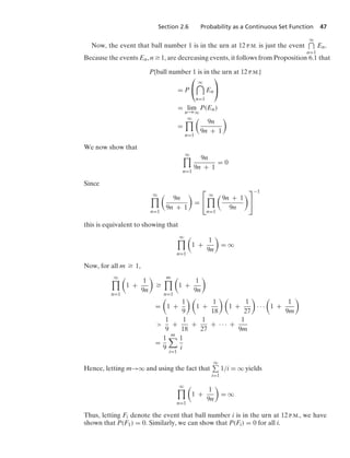
61. 46 Chapter 2 Axioms of Probability
EXAMPLE 6a Probability and a paradox
Suppose that we possess an infinitely large urn and an infinite collection of balls
labeled ball number 1, number 2, number 3, and so on. Consider an experiment per-
formed as follows: At 1 minute to 12 P.M., balls numbered 1 through 10 are placed
in the urn and ball number 10 is withdrawn. (Assume that the withdrawal takes
no time.) At 1
2 minute to 12 P.M., balls numbered 11 through 20 are placed in the
urn and ball number 20 is withdrawn. At 1
4 minute to 12 P.M., balls numbered 21
through 30 are placed in the urn and ball number 30 is withdrawn. At 1
8 minute
to 12 P.M., and so on. The question of interest is, How many balls are in the urn at
12 P.M.?
The answer to this question is clearly that there is an infinite number of
balls in the urn at 12 P.M., since any ball whose number is not of the form 10n,
n Ú 1, will have been placed in the urn and will not have been withdrawn before
12 P.M. Hence, the problem is solved when the experiment is performed as
described.
However, let us now change the experiment and suppose that at 1 minute to 12 P.M.
balls numbered 1 through 10 are placed in the urn and ball number 1 is withdrawn; at
1
2 minute to 12 P.M., balls numbered 11 through 20 are placed in the urn and ball num-
ber 2 is withdrawn; at 1
4 minute to 12 P.M., balls numbered 21 through 30 are placed
in the urn and ball number 3 is withdrawn; at 1
8 minute to 12 P.M., balls numbered 31
through 40 are placed in the urn and ball number 4 is withdrawn, and so on. For this
new experiment, how many balls are in the urn at 12 P.M.?
Surprisingly enough, the answer now is that the urn is empty at 12 P.M. For, consider
any ball—say, ball number n. At some time prior to 12 P.M. [in particular, at
1
2
n−1
minutes to 12 P.M.], this ball would have been withdrawn from the urn. Hence, for
each n, ball number n is not in the urn at 12 P.M.; therefore, the urn must be empty at
that time.
We see then, from the preceding discussion that the manner in which the balls are
withdrawn makes a difference. For, in the first case only balls numbered 10n, n Ú 1,
are ever withdrawn, whereas in the second case all of the balls are eventually with-
drawn. Let us now suppose that whenever a ball is to be withdrawn, that ball is
randomly selected from among those present. That is, suppose that at 1 minute to
12 P.M. balls numbered 1 through 10 are placed in the urn and a ball is randomly
selected and withdrawn, and so on. In this case, how many balls are in the urn at
12 P.M.?
Solution. We shall show that, with probability 1, the urn is empty at 12 P.M. Let us
first consider ball number 1. Define En to be the event that ball number 1 is still in
the urn after the first n withdrawals have been made. Clearly,
P(En) =
9 · 18 · 27 · · · (9n)
10 · 19 · 28 · · · (9n + 1)
[To understand this equation, just note that if ball number 1 is still to be in the
urn after the first n withdrawals, the first ball withdrawn can be any one of 9, the
second any one of 18 (there are 19 balls in the urn at the time of the second with-
drawal, one of which must be ball number 1), and so on. The denominator is similarly
obtained.]

62. Section 2.6 Probability as a Continuous Set Function 47
Now, the event that ball number 1 is in the urn at 12 P.M. is just the event
q
n=1
En.
Because the events En, n Ú 1, are decreasing events, it follows from Proposition 6.1 that
P{ball number 1 is in the urn at 12 P.M.}
= P
⎛
⎝
q
n=1
En
⎞
⎠
= lim
n→q
P(En)
=
q
n=1
9n
9n + 1
We now show that
q
n=1
9n
9n + 1
= 0
Since
q
n=1
9n
9n + 1
=
⎡
⎣
q
n=1
9n + 1
9n
⎤
⎦
−1
this is equivalent to showing that
q
n=1
1 +
1
9n
= q
Now, for all m Ú 1,
q
n=1
1 +
1
9n
Ú
m
n=1
1 +
1
9n
=
1 +
1
9
1 +
1
18
1 +
1
27
· · ·
1 +
1
9m
1
9
+
1
18
+
1
27
+ · · · +
1
9m
=
1
9
m
i=1
1
i
Hence, letting m→q and using the fact that
q
i=1
1/i = q yields
q
n=1
1 +
1
9n
= q
Thus, letting Fi denote the event that ball number i is in the urn at 12 P.M., we have
shown that P(F1) = 0. Similarly, we can show that P(Fi) = 0 for all i.

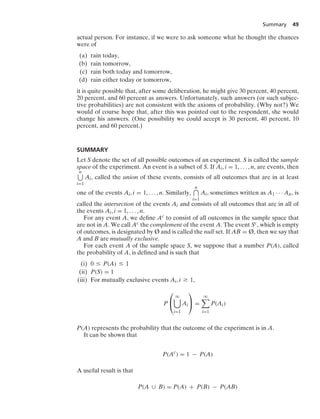
63. 48 Chapter 2 Axioms of Probability
(For instance, the same reasoning shows that P(Fi) =
q
$
n=2
[9n/(9n + 1)] for i =
11, 12, ... , 20.) Therefore, the probability that the urn is not empty at 12 P.M., P
q
1
Fi
,
satisfies
P
⎛
⎝
q
1
Fi
⎞
⎠ …
q
1
P(Fi) = 0
by Boole’s inequality. (See Self-Test Exercise 14.)
Thus, with probability 1, the urn will be empty at 12 P.M. .
2.7 PROBABILITY AS A MEASURE OF BELIEF
Thus far we have interpreted the probability of an event of a given experiment as
being a measure of how frequently the event will occur when the experiment is con-
tinually repeated. However, there are also other uses of the term probability. For
instance, we have all heard such statements as “It is 90 percent probable that Shake-
speare actually wrote Hamlet” or “The probability that Oswald acted alone in assas-
sinating Kennedy is .8.” How are we to interpret these statements?
The most simple and natural interpretation is that the probabilities referred to
are measures of the individual’s degree of belief in the statements that he or she
is making. In other words, the individual making the foregoing statements is quite
certain that Oswald acted alone and is even more certain that Shakespeare wrote
Hamlet. This interpretation of probability as being a measure of the degree of one’s
belief is often referred to as the personal or subjective view of probability.
It seems logical to suppose that a “measure of the degree of one’s belief” should
satisfy all of the axioms of probability. For example, if we are 70 percent certain that
Shakespeare wrote Julius Caesar and 10 percent certain that it was actually Mar-
lowe, then it is logical to suppose that we are 80 percent certain that it was either
Shakespeare or Marlowe. Hence, whether we interpret probability as a measure of
belief or as a long-run frequency of occurrence, its mathematical properties remain
unchanged.
EXAMPLE 7a
Suppose that, in a 7-horse race, you feel that each of the first 2 horses has a 20 percent
chance of winning, horses 3 and 4 each have a 15 percent chance, and the remaining
3 horses have a 10 percent chance each. Would it be better for you to wager at even
money that the winner will be one of the first three horses or to wager, again at even
money, that the winner will be one of the horses 1, 5, 6, and 7?
Solution. On the basis of your personal probabilities concerning the outcome of
the race, your probability of winning the first bet is .2 + .2 + .15 = .55, whereas
it is .2 + .1 + .1 + .1 = .5 for the second bet. Hence, the first wager is more
attractive. .
Note that, in supposing that a person’s subjective probabilities are always consis-
tent with the axioms of probability, we are dealing with an idealized rather than an

64. Summary 49
actual person. For instance, if we were to ask someone what he thought the chances
were of
(a) rain today,
(b) rain tomorrow,
(c) rain both today and tomorrow,
(d) rain either today or tomorrow,
it is quite possible that, after some deliberation, he might give 30 percent, 40 percent,
20 percent, and 60 percent as answers. Unfortunately, such answers (or such subjec-
tive probabilities) are not consistent with the axioms of probability. (Why not?) We
would of course hope that, after this was pointed out to the respondent, she would
change his answers. (One possibility we could accept is 30 percent, 40 percent, 10
percent, and 60 percent.)
SUMMARY
Let S denote the set of all possible outcomes of an experiment. S is called the sample
space of the experiment. An event is a subset of S. If Ai, i = 1, ... , n, are events, then
n
i=1
Ai, called the union of these events, consists of all outcomes that are in at least
one of the events Ai, i = 1, ... , n. Similarly,
n
i=1
Ai, sometimes written as A1 · · · An, is
called the intersection of the events Ai and consists of all outcomes that are in all of
the events Ai, i = 1, ... , n.
For any event A, we define Ac to consist of all outcomes in the sample space that
are not in A. We call Ac the complement of the event A. The event Sc, which is empty
of outcomes, is designated by Ø and is called the null set. If AB = Ø, then we say that
A and B are mutually exclusive.
For each event A of the sample space S, we suppose that a number P(A), called
the probability of A, is defined and is such that
(i) 0 … P(A) … 1
(ii) P(S) = 1
(iii) For mutually exclusive events Ai, i Ú 1,
P
⎛
⎝
q
i=1
Ai
⎞
⎠ =
q
i=1
P(Ai)
P(A) represents the probability that the outcome of the experiment is in A.
It can be shown that
P(Ac
) = 1 − P(A)
A useful result is that
P(A ∪ B) = P(A) + P(B) − P(AB)

65. 50 Chapter 2 Axioms of Probability
which can be generalized to give
P
⎛
⎝
n
i=1
Ai
⎞
⎠ =
n
i=1
P(Ai) −
ij
P(AiAj) +
ijk
P(AiAjAk)
+ · · · + (−1)n+1
P(A1 · · · An)
If S is finite and each one point set is assumed to have equal probability, then
P(A) =
|A|
|S|
where |E| denotes the number of outcomes in the event E.
P(A) can be interpreted either as a long-run relative frequency or as a measure of
one’s degree of belief.
PROBLEMS
1. A box contains 3 marbles: 1 red, 1 green, and 1
blue. Consider an experiment that consists of tak-
ing 1 marble from the box and then replacing it
in the box and drawing a second marble from the
box. Describe the sample space. Repeat when the
second marble is drawn without replacing the first
marble.
2. In an experiment, die is rolled continually until a
6 appears, at which point the experiment stops.
What is the sample space of this experiment? Let
En denote the event that n rolls are necessary to
complete the experiment. What points of the sam-
ple space are contained in En? What is
q
1
En
c
?
3. Two dice are thrown. Let E be the event that the
sum of the dice is odd, let F be the event that
at least one of the dice lands on 1, and let G be
the event that the sum is 5. Describe the events
EF, E ∪ F, FG, EFc, and EFG.
4. A, B, and C take turns flipping a coin. The first one
to get a head wins. The sample space of this exper-
iment can be defined by
S =
%
1, 01, 001, 0001, ... ,
0000 · · ·
(a) Interpret the sample space.
(b) Define the following events in terms of S:
(i) A wins = A.
(ii) B wins = B.
(iii) (A ∪ B)c.
Assume that A flips first, then B, then C,
then A, and so on.
5. A system is comprised of 5 components, each of
which is either working or failed. Consider an
experiment that consists of observing the status of
each component, and let the outcome of the exper-
iment be given by the vector (x1, x2, x3, x4, x5),
where xi is equal to 1 if component i is working
and is equal to 0 if component i is failed.
(a) How many outcomes are in the sample space
of this experiment?
(b) Suppose that the system will work if compo-
nents 1 and 2 are both working, or if compo-
nents 3 and 4 are both working, or if compo-
nents 1, 3, and 5 are all working. Let W be the
event that the system will work. Specify all the
outcomes in W.
(c) Let A be the event that components 4 and 5
are both failed. How many outcomes are con-
tained in the event A?
(d) Write out all the outcomes in the event AW.
6. A hospital administrator codes incoming patients
suffering gunshot wounds according to whether
they have insurance (coding 1 if they do and 0
if they do not) and according to their condition,
which is rated as good (g), fair (f), or serious (s).
Consider an experiment that consists of the coding
of such a patient.
(a) Give the sample space of this experiment.
(b) Let A be the event that the patient is in serious
condition. Specify the outcomes in A.
(c) Let B be the event that the patient is unin-
sured. Specify the outcomes in B.
(d) Give all the outcomes in the event Bc ∪ A.
7. Consider an experiment that consists of determin-
ing the type of job—either blue-collar or white-
collar—and the political affiliation—Republican,
Democratic, or Independent—of the 15 members
of an adult soccer team. How many outcomes are
(a) in the sample space?
(b) in the event that at least one of the team mem-
bers is a blue-collar worker?

66. Problems 51
(c) in the event that none of the team members
considers himself or herself an Independent?
8. Suppose that A and B are mutually exclusive
events for which P(A) = .3 and P(B) = .5. What is
the probability that
(a) either A or B occurs?
(b) A occurs but B does not?
(c) both A and B occur?
9. A retail establishment accepts either the American
Express or the VISA credit card. A total of 24 per-
cent of its customers carry an American Express
card, 61 percent carry a VISA card, and 11 per-
cent carry both cards. What percentage of its cus-
tomers carry a credit card that the establishment
will accept?
10. Sixty percent of the students at a certain school
wear neither a ring nor a necklace. Twenty per-
cent wear a ring and 30 percent wear a necklace.
If one of the students is chosen randomly, what is
the probability that this student is wearing
(a) a ring or a necklace?
(b) a ring and a necklace?
11. A total of 28 percent of American males smoke
cigarettes, 7 percent smoke cigars, and 5 percent
smoke both cigars and cigarettes.
(a) What percentage of males smokes neither
cigars nor cigarettes?
(b) What percentage smokes cigars but not
cigarettes?
12. An elementary school is offering 3 language
classes: one in Spanish, one in French, and one in
German. The classes are open to any of the 100
students in the school. There are 28 students in the
Spanish class, 26 in the French class, and 16 in the
German class. There are 12 students that are in
both Spanish and French, 4 that are in both Span-
ish and German, and 6 that are in both French and
German. In addition, there are 2 students taking
all 3 classes.
(a) If a student is chosen randomly, what is the
probability that he or she is not in any of the
language classes?
(b) If a student is chosen randomly, what is the
probability that he or she is taking exactly one
language class?
(c) If 2 students are chosen randomly, what is the
probability that at least 1 is taking a language
class?
13. A certain town with a population of 100,000 has
3 newspapers: I, II, and III. The proportions of
townspeople who read these papers are as follows:
I: 10 percent I and II: 8 percent I and II and
III: 1 percent
II: 30 percent I and III: 2 percent
III: 5 percent II and III: 4 percent
(The list tells us, for instance, that 8000 people
read newspapers I and II.)
(a) Find the number of people who read only one
newspaper.
(b) How many people read at least two
newspapers?
(c) If I and III are morning papers and II is an
evening paper, how many people read at least
one morning paper plus an evening paper?
(d) How many people do not read any
newspapers?
(e) How many people read only one morning
paper and one evening paper?
14. The following data were given in a study of a group
of 1000 subscribers to a certain magazine: In ref-
erence to job, marital status, and education, there
were 312 professionals, 470 married persons, 525
college graduates, 42 professional college gradu-
ates, 147 married college graduates, 86 married
professionals, and 25 married professional college
graduates. Show that the numbers reported in the
study must be incorrect.
Hint: Let M, W, and G denote, respectively, the
set of professionals, married persons, and college
graduates. Assume that one of the 1000 persons
is chosen at random, and use Proposition 4.4 to
show that if the given numbers are correct, then
P(M ∪ W ∪ G) 1.
15. If it is assumed that all
52
5
poker hands are
equally likely, what is the probability of being dealt
(a) a flush? (A hand is said to be a flush if all 5
cards are of the same suit.)
(b) one pair? (This occurs when the cards have
denominations a, a, b, c, d, where a, b, c, and
d are all distinct.)
(c) two pairs? (This occurs when the cards have
denominations a, a, b, b, c, where a, b, and c
are all distinct.)
(d) three of a kind? (This occurs when the cards
have denominations a, a, a, b, c, where a, b,
and c are all distinct.)
(e) four of a kind? (This occurs when the cards
have denominations a, a, a, a, b.)
16. Poker dice is played by simultaneously rolling 5
dice. Show that
(a) P{no two alike} = .0926;
(b) P{one pair} = .4630;
(c) P{two pair} = .2315;
(d) P{three alike} = .1543;
(e) P{full house} = .0386;
(f) P{four alike} = .0193;
(g) P{five alike} = .0008.
17. If 8 rooks (castles) are randomly placed on a
chessboard, compute the probability that none of
the rooks can capture any of the others. That is,

67. 52 Chapter 2 Axioms of Probability
compute the probability that no row or file con-
tains more than one rook.
18. Two cards are randomly selected from an ordinary
playing deck. What is the probability that they
form a blackjack? That is, what is the probability
that one of the cards is an ace and the other one is
either a ten, a jack, a queen, or a king?
19. Two symmetric dice have both had two of their
sides painted red, two painted black, one painted
yellow, and the other painted white. When this
pair of dice is rolled, what is the probability that
both dice land with the same color face up?
20. Suppose that you are playing blackjack against a
dealer. In a freshly shuffled deck, what is the prob-
ability that neither you nor the dealer is dealt a
blackjack?
21. A small community organization consists of 20
families, of which 4 have one child, 8 have two chil-
dren, 5 have three children, 2 have four children,
and 1 has five children.
(a) If one of these families is chosen at random,
what is the probability it has i children, i =
1, 2, 3, 4, 5?
(b) If one of the children is randomly chosen,
what is the probability that child comes from
a family having i children, i = 1, 2, 3, 4, 5?
22. Consider the following technique for shuffling a
deck of n cards: For any initial ordering of the
cards, go through the deck one card at a time and
at each card, flip a fair coin. If the coin comes
up heads, then leave the card where it is; if the
coin comes up tails, then move that card to the
end of the deck. After the coin has been flipped n
times, say that one round has been completed. For
instance, if n = 4 and the initial ordering is 1, 2, 3,
4, then if the successive flips result in the outcome
h, t, t, h, then the ordering at the end of the round
is 1, 4, 2, 3. Assuming that all possible outcomes of
the sequence of n coin flips are equally likely, what
is the probability that the ordering after one round
is the same as the initial ordering?
23. A pair of fair dice is rolled. What is the probabil-
ity that the second die lands on a higher value than
does the first?
24. If two dice are rolled, what is the probability that
the sum of the upturned faces equals i? Find it for
i = 2, 3, ... , 11, 12.
25. A pair of dice is rolled until a sum of either 5 or 7
appears. Find the probability that a 5 occurs first.
Hint: Let En denote the event that a 5 occurs on
the nth roll and no 5 or 7 occurs on the first n − 1
rolls. Compute P(En) and argue that
q
n=1
P(En) is
the desired probability.
26. The game of craps is played as follows: A player
rolls two dice. If the sum of the dice is either a 2,
3, or 12, the player loses; if the sum is either a 7
or an 11, the player wins. If the outcome is any-
thing else, the player continues to roll the dice until
she rolls either the initial outcome or a 7. If the 7
comes first, the player loses, whereas if the initial
outcome reoccurs before the 7 appears, the player
wins. Compute the probability of a player winning
at craps.
Hint: Let Ei denote the event that the initial out-
come is i and the player wins. The desired prob-
ability is
12
i=2
P(Ei). To compute P(Ei), define the
events Ei,n to be the event that the initial sum is
i and the player wins on the nth roll. Argue that
P(Ei) =
q
n=1
P(Ei,n).
27. An urn contains 3 red and 7 black balls. Players A
and B withdraw balls from the urn consecutively
until a red ball is selected. Find the probability that
A selects the red ball. (A draws the first ball, then
B, and so on. There is no replacement of the balls
drawn.)
28. An urn contains 5 red, 6 blue, and 8 green balls.
If a set of 3 balls is randomly selected, what is the
probability that each of the balls will be (a) of the
same color? (b) of different colors? Repeat under
the assumption that whenever a ball is selected, its
color is noted and it is then replaced in the urn
before the next selection. This is known as sam-
pling with replacement.
29. An urn contains n white and m black balls, where
n and m are positive numbers.
(a) If two balls are randomly withdrawn, what is
the probability that they are the same color?
(b) If a ball is randomly withdrawn and then
replaced before the second one is drawn, what
is the probability that the withdrawn balls are
the same color?
(c) Show that the probability in part (b) is always
larger than the one in part (a).
30. The chess clubs of two schools consist of, respec-
tively, 8 and 9 players. Four members from each
club are randomly chosen to participate in a con-
test between the two schools. The chosen play-
ers from one team are then randomly paired with
those from the other team, and each pairing plays
a game of chess. Suppose that Rebecca and her sis-
ter Elise are on the chess clubs at different schools.
What is the probability that
(a) Rebecca and Elise will be paired?
(b) Rebecca and Elise will be chosen to represent
their schools but will not play each other?
(c) either Rebecca or Elise will be chosen to
represent her school?

68. Problems 53
31. A 3-person basketball team consists of a guard, a
forward, and a center.
(a) If a person is chosen at random from each of
three different such teams, what is the proba-
bility of selecting a complete team?
(b) What is the probability that all 3 players
selected play the same position?
32. A group of individuals containing b boys and g
girls is lined up in random order; that is, each of
the (b + g)! permutations is assumed to be equally
likely. What is the probability that the person in
the ith position, 1 … i … b + g, is a girl?
33. A forest contains 20 elk, of which 5 are captured,
tagged, and then released. A certain time later, 4
of the 20 elk are captured. What is the probability
that 2 of these 4 have been tagged? What assump-
tions are you making?
34. The second Earl of Yarborough is reported to
have bet at odds of 1000 to 1 that a bridge hand
of 13 cards would contain at least one card that is
ten or higher. (By ten or higher we mean that a
card is either a ten, a jack, a queen, a king, or an
ace.) Nowadays, we call a hand that has no cards
higher than 9 a Yarborough. What is the proba-
bility that a randomly selected bridge hand is a
Yarborough?
35. Seven balls are randomly withdrawn from an urn
that contains 12 red, 16 blue, and 18 green balls.
Find the probability that
(a) 3 red, 2 blue, and 2 green balls are withdrawn;
(b) at least 2 red balls are withdrawn;
(c) all withdrawn balls are the same color;
(d) either exactly 3 red balls or exactly 3 blue balls
are withdrawn.
36. Two cards are chosen at random from a deck of 52
playing cards. What is the probability that they
(a) are both aces?
(b) have the same value?
37. An instructor gives her class a set of 10 problems
with the information that the final exam will con-
sist of a random selection of 5 of them. If a student
has figured out how to do 7 of the problems, what is
the probability that he or she will answer correctly
(a) all 5 problems?
(b) at least 4 of the problems?
38. There are n socks, 3 of which are red, in a drawer.
What is the value of n if, when 2 of the socks
are chosen randomly, the probability that they are
both red is 1
2 ?
39. There are 5 hotels in a certain town. If 3 people
check into hotels in a day, what is the probability
that they each check into a different hotel? What
assumptions are you making?
40. A town contains 4 people who repair televisions.
If 4 sets break down, what is the probability that
exactly i of the repairers are called? Solve the
problem for i = 1, 2, 3, 4. What assumptions are
you making?
41. If a die is rolled 4 times, what is the probability that
6 comes up at least once?
42. Two dice are thrown n times in succession. Com-
pute the probability that double 6 appears at least
once. How large need n be to make this probability
at least 1
2 ?
43. (a) If N people, including A and B, are randomly
arranged in a line, what is the probability that
A and B are next to each other?
(b) What would the probability be if the people
were randomly arranged in a circle?
44. Five people, designated as A, B, C, D, E, are
arranged in linear order. Assuming that each pos-
sible order is equally likely, what is the probabil-
ity that
(a) there is exactly one person between A and B?
(b) there are exactly two people between A
and B?
(c) there are three people between A and B?
45. A woman has n keys, of which one will open
her door.
(a) If she tries the keys at random, discarding
those that do not work, what is the probability
that she will open the door on her kth try?
(b) What if she does not discard previously tried
keys?
46. How many people have to be in a room in order
that the probability that at least two of them cele-
brate their birthday in the same month is at least
1
2 ? Assume that all possible monthly outcomes are
equally likely.
47. If there are 12 strangers in a room, what is the
probability that no two of them celebrate their
birthday in the same month?
48. Given 20 people, what is the probability that,
among the 12 months in the year, there are 4
months containing exactly 2 birthdays and 4 con-
taining exactly 3 birthdays?
49. A group of 6 men and 6 women is randomly
divided into 2 groups of size 6 each. What is the
probability that both groups will have the same
number of men?
50. In a hand of bridge, find the probability that you
have 5 spades and your partner has the remain-
ing 8.
51. Suppose that n balls are randomly distributed into
N compartments. Find the probability that m balls
will fall into the first compartment. Assume that all
Nn arrangements are equally likely.

69. 54 Chapter 2 Axioms of Probability
52. A closet contains 10 pairs of shoes. If 8 shoes
are randomly selected, what is the probability that
there will be
(a) no complete pair?
(b) exactly 1 complete pair?
53. If 4 married couples are arranged in a row, find the
probability that no husband sits next to his wife.
54. Compute the probability that a bridge hand is void
in at least one suit. Note that the answer is not
4
1
39
13
52
13
(Why not?)
Hint: Use Proposition 4.4.
55. Compute the probability that a hand of 13 cards
contains
(a) the ace and king of at least one suit;
(b) all 4 of at least 1 of the 13 denominations.
56. Two players play the following game: Player A
chooses one of the three spinners pictured in
Figure 2.6, and then player B chooses one of the
remaining two spinners. Both players then spin
their spinner, and the one that lands on the higher
number is declared the winner. Assuming that
each spinner is equally likely to land in any of its
3 regions, would you rather be player A or player
B? Explain your answer!
9 5
1
a
3 8
4
b
7 6
2
c
FIGURE 2.6: Spinners
THEORETICAL EXERCISES
Prove the following relations:
1. EF ( E ( E ∪ F.
2. If E ( F, then Fc ( Ec.
3. F = FE ∪ FEc and E ∪ F = E ∪ EcF.
4.
q
1
Ei
F =
q
1
EiF and
q
1
Ei
∪ F =
q
1
(Ei ∪ F).

70. Theoretical Exercises 55
5. For any sequence of events E1, E2, ..., define a
new sequence F1, F2, ... of disjoint events (that is,
events such that FiFj = Ø whenever i Z j) such
that for all n Ú 1,
n
1
Fi =
n
1
Ei
6. Let E, F, and G be three events. Find expressions
for the events so that, of E, F, and G,
(a) only E occurs;
(b) both E and G, but not F, occur;
(c) at least one of the events occurs;
(d) at least two of the events occur;
(e) all three events occur;
(f) none of the events occurs;
(g) at most one of the events occurs;
(h) at most two of the events occur;
(i) exactly two of the events occur;
(j) at most three of the events occur.
7. Find the simplest expression for the following
events:
(a) (E ∪ F)(E ∪ Fc);
(b) (E ∪ F)(Ec ∪ F)(E ∪ Fc);
(c) (E ∪ F)(F ∪ G).
8. Let S be a given set. If, for some k 0,
S1, S2, ... , Sk are mutually exclusive nonempty
subsets of S such that
k
i=1
Si = S, then we
call the set {S1, S2, ... , Sk} a partition of S. Let
Tn denote the number of different partitions of
{1, 2, ... , n}. Thus, T1 = 1 (the only partition being
S1 = {1}) and T2 = 2 (the two partitions being
{{1, 2, }}, {{1}, {2}}).
(a) Show, by computing all partitions, that T3 =
5, T4 = 15.
(b) Show that
Tn+1 = 1 +
n
k=1
n
k
Tk
and use this equation to compute T10.
Hint: One way of choosing a partition of n + 1
items is to call one of the items special. Then we
obtain different partitions by first choosing k, k =
0, 1, ... , n, then a subset of size n − k of the non-
special items, and then any of the Tk partitions of
the remaining k nonspecial items. By adding the
special item to the subset of size n − k, we obtain
a partition of all n + 1 items.
9. Suppose that an experiment is performed n times.
For any event E of the sample space, let n(E)
denote the number of times that event E occurs
and define f(E) = n(E)/n. Show that f(·) satisfies
Axioms 1, 2, and 3.
10. Prove that P(E ∪ F ∪ G) = P(E) + P(F) +
P(G) − P(EcFG) − P(EFcG) − P(EFGc) −
2P(EFG).
11. If P(E) = .9 and P(F) = .8, show that P(EF) Ú .7.
In general, prove Bonferroni’s inequality, namely,
P(EF) Ú P(E) + P(F) − 1
12. Show that the probability that exactly one of the
events E or F occurs equals P(E) + P(F) −
2P(EF).
13. Prove that P(EFc) = P(E) − P(EF).
14. Prove Proposition 4.4 by mathematical induction.
15. An urn contains M white and N black balls. If a
random sample of size r is chosen, what is the prob-
ability that it contains exactly k white balls?
16. Use induction to generalize Bonferroni’s inequal-
ity to n events. That is, show that
P(E1E2 · · · En) Ú P(E1) + · · · + P(En) − (n − 1)
17. Consider the matching problem, Example 5m, and
define AN to be the number of ways in which the
N men can select their hats so that no man selects
his own. Argue that
AN = (N − 1)(AN−1 + AN−2)
This formula, along with the boundary conditions
A1 = 0, A2 = 1, can then be solved for AN, and
the desired probability of no matches would be
AN/N!.
Hint: After the first man selects a hat that is not his
own, there remain N − 1 men to select among a set
of N − 1 hats that does not contain the hat of one
of these men. Thus, there is one extra man and one
extra hat. Argue that we can get no matches either
with the extra man selecting the extra hat or with
the extra man not selecting the extra hat.
18. Let fn denote the number of ways of tossing a coin
n times such that successive heads never appear.
Argue that
fn = fn−1 + fn−2 n Ú 2, where f0 K 1, f1 K 2
Hint: How many outcomes are there that start
with a head, and how many start with a tail? If
Pn denotes the probability that successive heads
never appear when a coin is tossed n times, find
Pn (in terms of fn) when all possible outcomes of
the n tosses are assumed equally likely. Compute
P10.
19. An urn contains n red and m blue balls. They are
withdrawn one at a time until a total of r, r … n,

71. 56 Chapter 2 Axioms of Probability
red balls have been withdrawn. Find the probabil-
ity that a total of k balls are withdrawn.
Hint: A total of k balls will be withdrawn if there
are r − 1 red balls in the first k − 1 withdrawals
and the kth withdrawal is a red ball.
20. Consider an experiment whose sample space con-
sists of a countably infinite number of points.
Show that not all points can be equally likely.
Can all points have a positive probability of
occurring?
∗21. Consider Example 5o, which is concerned with the
number of runs of wins obtained when n wins and
m losses are randomly permuted. Now
consider the total number of runs—that is, win
runs plus loss runs—and show that
P{2k runs} = 2
m − 1
k − 1
n − 1
k − 1
m + n
n
P{2k + 1 runs}
=
m − 1
k − 1
n − 1
k
+
m − 1
k
n − 1
k − 1
m + n
n
SELF-TEST PROBLEMS AND EXERCISES
1. A cafeteria offers a three-course meal consisting
of an entree, a starch, and a dessert. The possible
choices are given in the following table:
Course Choices
Entree Chicken or roast beef
Starch Pasta or rice or potatoes
Dessert Ice cream or Jello or apple pie or a peach
A person is to choose one course from each cate-
gory.
(a) How many outcomes are in the sample space?
(b) Let A be the event that ice cream is chosen.
How many outcomes are in A?
(c) Let B be the event that chicken is chosen.
How many outcomes are in B?
(d) List all the outcomes in the event AB.
(e) Let C be the event that rice is chosen. How
many outcomes are in C?
(f) List all the outcomes in the event ABC.
2. A customer visiting the suit department of a cer-
tain store will purchase a suit with probability .22,
a shirt with probability .30, and a tie with proba-
bility .28. The customer will purchase both a suit
and a shirt with probability .11, both a suit and a
tie with probability .14, and both a shirt and a tie
with probability .10. A customer will purchase all 3
items with probability .06. What is the probability
that a customer purchases
(a) none of these items?
(b) exactly 1 of these items?
3. A deck of cards is dealt out. What is the proba-
bility that the 14th card dealt is an ace? What is
the probability that the first ace occurs on the 14th
card?
4. Let A denote the event that the midtown temper-
ature in Los Angeles is 70◦F, and let B denote the
event that the midtown temperature in New York
is 70◦F. Also, let C denote the event that the max-
imum of the midtown temperatures in New York
and in Los Angeles is 70◦F. If P(A) = .3, P(B) =
.4, and P(C) = .2, find the probability that the min-
imum of the two midtown temperatures is 70◦F.
5. An ordinary deck of 52 cards is shuffled. What is
the probability that the top four cards have
(a) different denominations?
(b) different suits?
6. Urn A contains 3 red and 3 black balls, whereas
urn B contains 4 red and 6 black balls. If a ball is
randomly selected from each urn, what is the prob-
ability that the balls will be the same color?
7. In a state lottery, a player must choose 8 of the
numbers from 1 to 40. The lottery commission
then performs an experiment that selects 8 of these
40 numbers. Assuming that the choice of the lot-
tery commission is equally likely to be any of the
40
8
combinations, what is the probability that a
player has
(a) all 8 of the numbers selected by the lottery
commission?
(b) 7 of the numbers selected by the lottery com-
mission?
(c) at least 6 of the numbers selected by the lot-
tery commission?
8. From a group of 3 freshmen, 4 sophomores, 4
juniors, and 3 seniors a committee of size 4 is ran-
domly selected. Find the probability that the com-
mittee will consist of
(a) 1 from each class;
(b) 2 sophomores and 2 juniors;
(c) only sophomores or juniors.

72. Self -Test Problems and Exercises 57
9. For a finite set A, let N(A) denote the number of
elements in A.
(a) Show that
N(A ∪ B) = N(A) + N(B) − N(AB)
(b) More generally, show that
N
⎛
⎝
n
i=1
Ai
⎞
⎠ =
i
N(Ai) −
ij
N(AiAj)
+ · · · + (−1)n+1
N(A1 · · · An)
10. Consider an experiment that consists of six horses,
numbered 1 through 6, running a race, and sup-
pose that the sample space consists of the 6! pos-
sible orders in which the horses finish. Let A be
the event that the number-1 horse is among the
top three finishers, and let B be the event that the
number-2 horse comes in second. How many out-
comes are in the event A ∪ B?
11. A 5-card hand is dealt from a well-shuffled deck of
52 playing cards. What is the probability that the
hand contains at least one card from each of the
four suits?
12. A basketball team consists of 6 frontcourt and
4 backcourt players. If players are divided into
roommates at random, what is the probability that
there will be exactly two roommate pairs made up
of a backcourt and a frontcourt player?
13. Suppose that a person chooses a letter at random
from R E S E R V E and then chooses one at ran-
dom from V E R T I C A L. What is the probability
that the same letter is chosen?
14. Prove Boole’s inequality:
P
⎛
⎝
q
i=1
Ai
⎞
⎠ …
q
i=1
P(Ai)
15. Show that if P(Ai) = 1 for all i Ú 1, then
P
q
i=1
Ai
= 1.
16. Let Tk(n) denote the number of partitions of the
set {1, ... , n} into k nonempty subsets, where 1 …
k … n. (See Theoretical Exercise 8 for the defini-
tion of a partition.) Argue that
Tk(n) = kTk(n − 1) + Tk−1(n − 1)
Hint: In how many partitions is {1} a subset, and in
how many is 1 an element of a subset that contains
other elements?
17. Five balls are randomly chosen, without replace-
ment, from an urn that contains 5 red, 6 white, and
7 blue balls. Find the probability that at least one
ball of each color is chosen.
18. Four red, 8 blue, and 5 green balls are randomly
arranged in a line.
(a) What is the probability that the first 5 balls are
blue?
(b) What is the probability that none of the first 5
balls are blue?
(c) What is the probability that the final 3 balls
are differently colored.
(d) What is the probability that all the red balls
are together?
19. Ten cards are randomly chosen from a deck of 52
cards that consists of 13 cards of each of 4 different
suits. Each of the selected cards is put in one of 4
piles, depending on the suit of the card.
(a) What is the probability that the largest pile
has 4 cards, the next largest has 3, the next
largest has 2, and the smallest has 1 card?
(b) What is the probability that two of the piles
have 3 cards, one has 4 cards, and one has no
cards?
20. Balls are randomly removed from an urn initially
containing 20 red and 10 blue balls. What is the
probability that all of the red balls are removed
before all of the blue ones have been removed?

73. C H A P T E R 3
Conditional Probability and Independence
3.1 INTRODUCTION
3.2 CONDITIONAL PROBABILITIES
3.3 BAYES’S FORMULA
3.4 INDEPENDENT EVENTS
3.5 P(·|F ) IS A PROBABILITY
3.1 INTRODUCTION
In this chapter, we introduce one of the most important concepts in probability theory,
that of conditional probability. The importance of this concept is twofold. In the first
place, we are often interested in calculating probabilities when some partial informa-
tion concerning the result of an experiment is available; in such a situation, the desired
probabilities are conditional. Second, even when no partial information is available,
conditional probabilities can often be used to compute the desired probabilities more
easily.
3.2 CONDITIONAL PROBABILITIES
Suppose that we toss 2 dice, and suppose that each of the 36 possible outcomes is
equally likely to occur and hence has probability 1
36. Suppose further that we observe
that the first die is a 3. Then, given this information, what is the probability that the
sum of the 2 dice equals 8? To calculate this probability, we reason as follows: Given
that the initial die is a 3, there can be at most 6 possible outcomes of our experiment,
namely, (3, 1), (3, 2), (3, 3), (3, 4), (3, 5), and (3, 6). Since each of these outcomes
originally had the same probability of occurring, the outcomes should still have equal
probabilities. That is, given that the first die is a 3, the (conditional) probability of
each of the outcomes (3, 1), (3, 2), (3, 3), (3, 4), (3, 5), and (3, 6) is 1
6, whereas the
(conditional) probability of the other 30 points in the sample space is 0. Hence, the
desired probability will be 1
6 .
If we let E and F denote, respectively, the event that the sum of the dice is 8 and the
event that the first die is a 3, then the probability just obtained is called the conditional
probability that E occurs given that F has occurred and is denoted by
P(E|F)
A general formula for P(E|F) that is valid for all events E and F is derived in the same
manner: If the event F occurs, then, in order for E to occur, it is necessary that the
actual occurrence be a point both in E and in F; that is, it must be in EF. Now, since
we know that F has occurred, it follows that F becomes our new, or reduced, sample
space; hence, the probability that the event EF occurs will equal the probability of
EF relative to the probability of F. That is, we have the following definition.
58

74. Section 3.2 Conditional Probabilities 59
Definition
If P(F) 0, then
P(E|F) =
P(EF)
P(F)
(2.1)
EXAMPLE 2a
A student is taking a one-hour-time-limit makeup examination. Suppose the proba-
bility that the student will finish the exam in less than x hours is x/2, for all 0 … x … 1.
Then, given that the student is still working after .75 hour, what is the conditional
probability that the full hour is used?
Solution. Let Lx denote the event that the student finishes the exam in less than x
hours, 0 … x … 1, and let F be the event that the student uses the full hour. Because
F is the event that the student is not finished in less than 1 hour,
P(F) = P(Lc
1) = 1 − P(L1) = .5
Now, the event that the student is still working at time .75 is the complement of the
event L.75, so the desired probability is obtained from
P(F|Lc
.75) =
P(FLc
.75)
P(Lc
.75)
=
P(F)
1 − P(L.75)
=
.5
.625
= .8
.
If each outcome of a finite sample space S is equally likely, then, conditional on
the event that the outcome lies in a subset F ( S, all outcomes in F become equally
likely. In such cases, it is often convenient to compute conditional probabilities of
the form P(E|F) by using F as the sample space. Indeed, working with this reduced
sample space often results in an easier and better understood solution. Our next few
examples illustrate this point.
EXAMPLE 2b
A coin is flipped twice. Assuming that all four points in the sample space S = {(h, h),
(h, t), (t, h), (t, t)} are equally likely, what is the conditional probability that both flips
land on heads, given that (a) the first flip lands on heads? (b) at least one flip lands
on heads?
Solution. Let B = {(h, h)} be the event that both flips land on heads; let F = {(h, h),
(h, t)} be the event that the first flip lands on heads; and let A = {(h, h), (h, t), (t, h)} be
the event that at least one flip lands on heads. The probability for (a) can be obtained
from

75. 60 Chapter 3 Conditional Probability and Independence
P(B|F) =
P(BF)
P(F)
=
P({(h, h)})
P({(h, h), (h, t)})
=
1/4
2/4
= 1/2
For (b), we have
P(B|A) =
P(BA)
P(A)
=
P({(h, h)})
P({(h, h), (h, t), (t, h)})
=
1/4
3/4
= 1/3
Thus, the conditional probability that both flips land on heads given that the first
one does is 1/2, whereas the conditional probability that both flips land on heads
given that at least one does is only 1/3. Many students initially find this latter result
surprising. They reason that, given that at least one flip lands on heads, there are
two possible results: Either they both land on heads or only one does. Their mistake,
however, is in assuming that these two possibilities are equally likely. For, initially,
there are 4 equally likely outcomes. Because the information that at least one flip
lands on heads is equivalent to the information that the outcome is not (t, t), we are
left with the 3 equally likely outcomes (h, h), (h, t), (t, h), only one of which results in
both flips landing on heads. .
EXAMPLE 2c
In the card game bridge, the 52 cards are dealt out equally to 4 players—called East,
West, North, and South. If North and South have a total of 8 spades among them,
what is the probability that East has 3 of the remaining 5 spades?
Solution. Probably the easiest way to compute the desired probability is to work
with the reduced sample space. That is, given that North–South have a total of 8
spades among their 26 cards, there remains a total of 26 cards, exactly 5 of them
being spades, to be distributed among the East–West hands. Since each distribution
is equally likely, it follows that the conditional probability that East will have exactly
3 spades among his or her 13 cards is
5
3
21
10
26
13
L .339 .
EXAMPLE 2d
A total of n balls are sequentially and randomly chosen, without replacement, from
an urn containing r red and b blue balls (n … r + b). Given that k of the n balls are
blue, what is the conditional probability that the first ball chosen is blue?

76. Section 3.2 Conditional Probabilities 61
Solution. If we imagine that the balls are numbered, with the blue balls having num-
bers 1 through b and the red balls b + 1 through b + r, then the outcome of the
experiment of selecting n balls without replacement is a vector of distinct integers
x1, ... , xn, where each xi is between 1 and r + b. Moreover, each such vector is equally
likely to be the outcome. So, given that the vector contains k blue balls (that is, it
contains k values between 1 and b), it follows that each of these outcomes is equally
likely. But because the first ball chosen is, therefore, equally likely to be any of the n
chosen balls, of which k are blue, it follows that the desired probability is k/n.
If we did not choose to work with the reduced sample space, we could have solved
the problem by letting B be the event that the first ball chosen is blue and Bk be the
event that a total of k blue balls are chosen. Then
P(B|Bk) =
P(BBk)
P(Bk)
=
P(Bk|B)P(B)
P(Bk)
Now, P(Bk|B) is the probability that a random choice of n − 1 balls from an urn
containing r red and b − 1 blue balls results in a total of k − 1 blue balls being
chosen; consequently,
P(Bk|B) =
b−1
k−1
r
n−k
r+b−1
n−1
Using the preceding formula along with
P(B) =
b
r + b
and the hypergeometric probability
P(Bk) =
b
k
r
n−k
r+b
n
again yields the result that
P(B|Bk) =
k
n .
Multiplying both sides of Equation (2.1) by P(F ), we obtain
P(EF ) = P(F)P(E|F ) (2.2)
In words, Equation (2.2) states that the probability that both E and F occur is equal
to the probability that F occurs multiplied by the conditional probability of E given
that F occurred. Equation (2.2) is often quite useful in computing the probability of
the intersection of events.
EXAMPLE 2e
Celine is undecided as to whether to take a French course or a chemistry course. She
estimates that her probability of receiving an A grade would be 1
2 in a French course
and 2
3 in a chemistry course. If Celine decides to base her decision on the flip of a fair
coin, what is the probability that she gets an A in chemistry?

77. 62 Chapter 3 Conditional Probability and Independence
Solution. (a) Let the event that Celine takes chemistry and A denote the event that
she receives an A in whatever course she takes, then the desired probability is P(CA),
which is calculated by using Equation (2.2) as follows:
P(CA) = P(C)P(A|C)
=
1
2
2
3
=
1
3 .
EXAMPLE 2f
Suppose that an urn contains 8 red balls and 4 white balls. We draw 2 balls from the
urn without replacement. (a) If we assume that at each draw each ball in the urn is
equally likely to be chosen, what is the probability that both balls drawn are red? (b)
Now suppose that the balls have different weights, with each red ball having weight r
and each white ball having weight w. Suppose that the probability that a given ball in
the urn is the next one selected is its weight divided by the sum of the weights of all
balls currently in the urn. Now what is the probability that both balls are red?
Solution. Let R1 and R2 denote, respectively, the events that the first and second
balls drawn are red. Now, given that the first ball selected is red, there are 7 remaining
red balls and 4 white balls, so P(R2|R1) = 7
11. As P(R1) is clearly 8
12, the desired
probability is
P(R1R2) = P(R1)P(R2|R1)
=
2
3
7
11
=
14
33
Of course, this probability could have been computed by P(R1R2) =
8
2
/
12
2
.
For part (b), we again let Ri be the event that the ith ball chosen is red and use
P(R1R2) = P(R1)P(R2|R1)
Now, number the red balls, and let Bi, i = 1, ... , 8 be the event that the first ball
drawn is red ball number i. Then
P(R1) = P(∪8
i=1Bi) =
8
i=1
P(Bi) = 8
r
8r + 4w
Moreover, given that the first ball is red, the urn then contains 7 red and 4 white balls.
Thus, by an argument similar to the preceding one,
P(R2|R1) =
7r
7r + 4w
Hence, the probability that both balls are red is
P(R1R2) =
8r
8r + 4w
7r
7r + 4w .
A generalization of Equation (2.2), which provides an expression for the probabil-
ity of the intersection of an arbitrary number of events, is sometimes referred to as
the multiplication rule.

78. Section 3.2 Conditional Probabilities 63
The multiplication rule
P(E1E2E3 · · · En) = P(E1)P(E2|E1)P(E3|E1E2) · · · P(En|E1 · · · En−1)
To prove the multiplication rule, just apply the definition of conditional probability
to its right-hand side, giving
P(E1)
P(E1E2)
P(E1)
P(E1E2E3)
P(E1E2)
· · ·
P(E1E2 · · · En)
P(E1E2 · · · En−1)
= P(E1E2 · · · En)
EXAMPLE 2g
In the match problem stated in Example 5m of Chapter 2, it was shown that PN, the
probability that there are no matches when N people randomly select from among
their own N hats, is given by
PN =
N
i=0
(−1)i
/i!
What is the probability that exactly k of the N people have matches?
Solution. Let us fix our attention on a particular set of k people and determine the
probability that these k individuals have matches and no one else does. Letting E
denote the event that everyone in this set has a match, and letting G be the event that
none of the other N − k people have a match, we have
P(EG) = P(E )P(G|E )
Now, let Fi, i = 1, ... , k, be the event that the ith member of the set has a match.
Then
P(E ) = P(F1F2 · · · Fk)
= P(F1)P(F2|F1)P(F3|F1F2) · · · P(Fk|F1 · · · Fk−1)
=
1
N
1
N − 1
1
N − 2
· · ·
1
N − k + 1
=
(N − k)!
N!
Given that everyone in the set of k has a match, the other N − k people will be
randomly choosing among their own N − k hats, so the probability that none of
them has a match is equal to the probability of no matches in a problem having N − k
people choosing among their own N − k hats. Therefore,
P(G|E ) = PN−k =
N−k
i=0
(−1)i
/i!
showing that the probability that a specified set of k people have matches and no one
else does is
P(EG) =
(N − k)!
N!
PN−k

79. 64 Chapter 3 Conditional Probability and Independence
Because there will be exactly k matches if the preceding is true for any of the
N
k
sets
of k individuals, the desired probability is
P(exactly k matches) = PN−k/k!
L e−1
/k! when N is large .
We will now employ the multiplication rule to obtain a second approach to solving
Example 5h(b) of Chapter 2.
EXAMPLE 2h
An ordinary deck of 52 playing cards is randomly divided into 4 piles of 13 cards each.
Compute the probability that each pile has exactly 1 ace.
Solution. Define events Ei, i = 1, 2, 3, 4, as follows:
E1 = {the ace of spades is in any one of the piles}
E2 = {the ace of spades and the ace of hearts are in different piles}
E3 = {the aces of spades, hearts, and diamonds are all in different piles}
E4 = {all 4 aces are in different piles}
The desired probability is P(E1E2E3E4), and by the multiplication rule,
P(E1E2E3E4) = P(E1)P(E2|E1)P(E3|E1E2)P(E4|E1E2E3)
Now,
P(E1) = 1
since E1 is the sample space S. Also,
P(E2|E1) =
39
51
since the pile containing the ace of spades will receive 12 of the remaining 51 cards,
and
P(E3|E1E2) =
26
50
since the piles containing the aces of spades and hearts will receive 24 of the remain-
ing 50 cards. Finally,
P(E4|E1E2E3) =
13
49
Therefore, the probability that each pile has exactly 1 ace is
P(E1E2E3E4) =
39 · 26 · 13
51 · 50 · 49
L .105
That is, there is approximately a 10.5 percent chance that each pile will contain an
ace. (Problem 13 gives another way of using the multiplication rule to solve this
problem.) .
Remarks. Our definition of P(E|F) is consistent with the interpretation of prob-
ability as being a long-run relative frequency. To see this, suppose that n repeti-
tions of the experiment are to be performed, where n is large. We claim that if

80. Section 3.3 Bayes’s Formula 65
we consider only those experiments in which F occurs, then P(E|F) will equal the
long-run proportion of them in which E also occurs. To verify this statement, note
that, since P(F) is the long-run proportion of experiments in which F occurs,
it follows that in the n repetitions of the experiment F will occur approximately
nP(F) times. Similarly, in approximately nP(EF) of these experiments both E and
F will occur. Hence, out of the approximately nP(F) experiments in which
F occurs, the proportion of them in which E also occurs is approximately
equal to
nP(EF)
nP(F)
=
P(EF)
P(F)
Because this approximation becomes exact as n becomes larger and larger, we have
the appropriate definition of P(E|F).
3.3 BAYES’S FORMULA
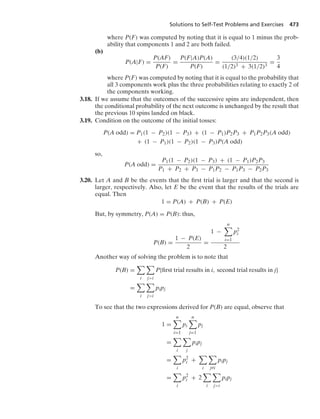
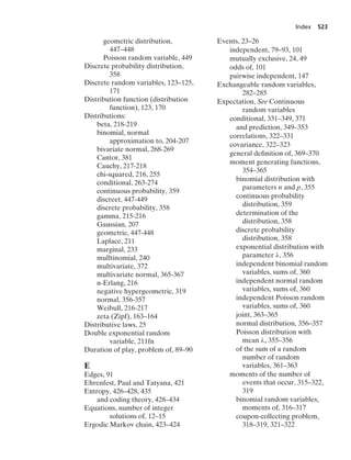
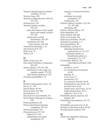
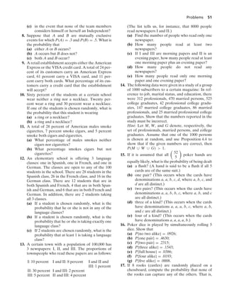
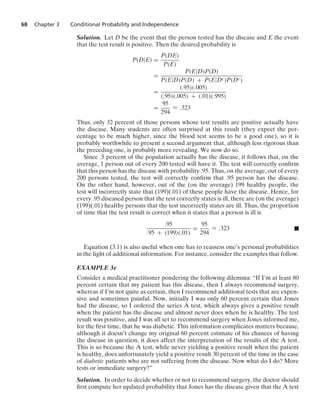
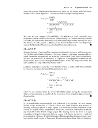
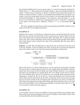
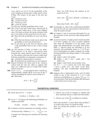
Let E and F be events. We may express E as
E = EF ∪ EFc
for, in order for an outcome to be in E, it must either be in both E and F or be in
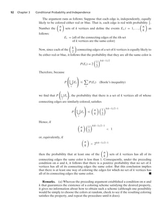
E but not in F. (See Figure 3.1.) As EF and EFc are clearly mutually exclusive, we
have, by Axiom 3,
P(E ) = P(EF ) + P(EFc)
= P(E|F )P(F ) + P(E|Fc)P(Fc)
= P(E|F )P(F ) + P(E|Fc)[1 − P(F)]
(3.1)
Equation (3.1) states that the probability of the event E is a weighted average of the
conditional probability of E given that F has occurred and the conditional proba-
bility of E given that F has not occurred—each conditional probability being given
as much weight as the event on which it is conditioned has of occurring. This is an
extremely useful formula, because its use often enables us to determine the prob-
ability of an event by first “conditioning” upon whether or not some second event
has occurred. That is, there are many instances in which it is difficult to compute the
probability of an event directly, but it is straightforward to compute it once we know
whether or not some second event has occurred. We illustrate this idea with some
examples.
E F
EF
EFc
FIGURE 3.1: E = EF ∪ EFc. EF = Shaded Area; EFc = Striped Area

81. 66 Chapter 3 Conditional Probability and Independence
EXAMPLE 3a (Part 1)
An insurance company believes that people can be divided into two classes: those
who are accident prone and those who are not. The company’s statistics show that
an accident-prone person will have an accident at some time within a fixed 1-year
period with probability .4, whereas this probability decreases to .2 for a person who is
not accident prone. If we assume that 30 percent of the population is accident prone,
what is the probability that a new policyholder will have an accident within a year of
purchasing a policy?
Solution. We shall obtain the desired probability by first conditioning upon whether
or not the policyholder is accident prone. Let A1 denote the event that the policy-
holder will have an accident within a year of purchasing the policy, and let A denote
the event that the policyholder is accident prone. Hence, the desired probability is
given by
P(A1) = P(A1|A)P(A) + P(A1|Ac
)P(Ac
)
= (.4)(.3) + (.2)(.7) = .26 .
EXAMPLE 3a (Part 2)
Suppose that a new policyholder has an accident within a year of purchasing a policy.
What is the probability that he or she is accident prone?
Solution. The desired probability is
P(A|A1) =
P(AA1)
P(A1)
=
P(A)P(A1|A)
P(A1)
=
(.3)(.4)
.26
=
6
13 .
EXAMPLE 3b
Consider the following game played with an ordinary deck of 52 playing cards: The
cards are shuffled and then turned over one at a time. At any time, the player can
guess that the next card to be turned over will be the ace of spades; if it is, then the
player wins. In addition, the player is said to win if the ace of spades has not yet
appeared when only one card remains and no guess has yet been made. What is a
good strategy? What is a bad strategy?
Solution. Every strategy has probability 1/52 of winning! To show this, we will use
induction to prove the stronger result that, for an n card deck, one of whose cards
is the ace of spades, the probability of winning is 1/n, no matter what strategy is
employed. Since this is clearly true for n = 1, assume it to be true for an n − 1
card deck, and now consider an n card deck. Fix any strategy, and let p denote the
probability that the strategy guesses that the first card is the ace of spades. Given that
it does, the player’s probability of winning is 1/n. If, however, the strategy does not
guess that the first card is the ace of spades, then the probability that the player wins
is the probability that the first card is not the ace of spades, namely, (n − 1)/n, multi-
plied by the conditional probability of winning given that the first card is not the ace
of spades. But this latter conditional probability is equal to the probability of winning

82. Section 3.3 Bayes’s Formula 67
when using an n − 1 card deck containing a single ace of spades; it is thus, by the
induction hypothesis, 1/(n − 1). Hence, given that the strategy does not guess the
first card, the probability of winning is
n − 1
n
1
n − 1
=
1
n
Thus, letting G be the event that the first card is guessed, we obtain
P{win} = P{win|G}P(G) + P{win|Gc
}(1 − P(G)) =
1
n
p +
1
n
(1 − p)
=
1
n
.
EXAMPLE 3c
In answering a question on a multiple-choice test, a student either knows the answer
or guesses. Let p be the probability that the student knows the answer and 1 − p
be the probability that the student guesses. Assume that a student who guesses at the
answer will be correct with probability 1/m, where m is the number of multiple-choice
alternatives. What is the conditional probability that a student knew the answer to a
question given that he or she answered it correctly?
Solution. Let C and K denote, respectively, the events that the student answers the
question correctly and the event that he or she actually knows the answer. Now,
P(K|C ) =
P(KC )
P(C )
=
P(C|K )P(K )
P(C|K )P(K ) + P(C|Kc)P(Kc)
=
p
p + (1/m)(1 − p)
=
mp
1 + (m − 1)p
For example, if m = 5, p = 1
2, then the probability that the student knew the answer
to a question he or she answered correctly is 5
6. .
EXAMPLE 3d
A laboratory blood test is 95 percent effective in detecting a certain disease when it
is, in fact, present. However, the test also yields a “false positive” result for 1 percent
of the healthy persons tested. (That is, if a healthy person is tested, then, with prob-
ability .01, the test result will imply that he or she has the disease.) If .5 percent of
the population actually has the disease, what is the probability that a person has the
disease given that the test result is positive?

83. 68 Chapter 3 Conditional Probability and Independence
Solution. Let D be the event that the person tested has the disease and E the event
that the test result is positive. Then the desired probability is
P(D|E) =
P(DE)
P(E)
=
P(E|D)P(D)
P(E|D)P(D) + P(E|Dc)P(Dc)
=
(.95)(.005)
(.95)(.005) + (.01)(.995)
=
95
294
L .323
Thus, only 32 percent of those persons whose test results are positive actually have
the disease. Many students are often surprised at this result (they expect the per-
centage to be much higher, since the blood test seems to be a good one), so it is
probably worthwhile to present a second argument that, although less rigorous than
the preceding one, is probably more revealing. We now do so.
Since .5 percent of the population actually has the disease, it follows that, on the
average, 1 person out of every 200 tested will have it. The test will correctly confirm
that this person has the disease with probability .95. Thus, on the average, out of every
200 persons tested, the test will correctly confirm that .95 person has the disease.
On the other hand, however, out of the (on the average) 199 healthy people, the
test will incorrectly state that (199)(.01) of these people have the disease. Hence, for
every .95 diseased person that the test correctly states is ill, there are (on the average)
(199)(.01) healthy persons that the test incorrectly states are ill. Thus, the proportion
of time that the test result is correct when it states that a person is ill is
.95
.95 + (199)(.01)
=
95
294
L .323 .
Equation (3.1) is also useful when one has to reassess one’s personal probabilities
in the light of additional information. For instance, consider the examples that follow.
EXAMPLE 3e
Consider a medical practitioner pondering the following dilemma: “If I’m at least 80
percent certain that my patient has this disease, then I always recommend surgery,
whereas if I’m not quite as certain, then I recommend additional tests that are expen-
sive and sometimes painful. Now, initially I was only 60 percent certain that Jones
had the disease, so I ordered the series A test, which always gives a positive result
when the patient has the disease and almost never does when he is healthy. The test
result was positive, and I was all set to recommend surgery when Jones informed me,
for the first time, that he was diabetic. This information complicates matters because,
although it doesn’t change my original 60 percent estimate of his chances of having
the disease in question, it does affect the interpretation of the results of the A test.
This is so because the A test, while never yielding a positive result when the patient
is healthy, does unfortunately yield a positive result 30 percent of the time in the case
of diabetic patients who are not suffering from the disease. Now what do I do? More
tests or immediate surgery?”
Solution. In order to decide whether or not to recommend surgery, the doctor should
first compute her updated probability that Jones has the disease given that the A test

84. Section 3.3 Bayes’s Formula 69
result was positive. Let D denote the event that Jones has the disease and E the event
that the A test result is positive. The desired conditional probability is then
P(D|E) =
P(DE)
P(E)
=
P(D)P(E|D)
P(E|D)P(D) + P(E|Dc)P(Dc)
=
(.6)1
1(.6) + (.3)(.4)
= .833
Note that we have computed the probability of a positive test result by conditioning
on whether or not Jones has the disease and then using the fact that, because Jones is
a diabetic, his conditional probability of a positive result given that he does not have
the disease, P(E|Dc), equals .3. Hence, as the doctor should now be over 80 percent
certain that Jones has the disease, she should recommend surgery. .
EXAMPLE 3f
At a certain stage of a criminal investigation, the inspector in charge is 60 percent con-
vinced of the guilt of a certain suspect. Suppose, however, that a new piece of evidence
which shows that the criminal has a certain characteristic (such as left-handedness,
baldness, or brown hair) is uncovered. If 20 percent of the population possesses this
characteristic, how certain of the guilt of the suspect should the inspector now be if it
turns out that the suspect has the characteristic?
Solution. Letting G denote the event that the suspect is guilty and C the event that
he possesses the characteristic of the criminal, we have
P(G|C) =
P(GC)
P(C)
=
P(C|G)P(G)
P(C|G)P(G) + P(C|Gc)P(Gc)
=
1(.6)
1(.6) + (.2)(.4)
L .882
where we have supposed that the probability of the suspect having the characteristic
if he is, in fact, innocent is equal to .2, the proportion of the population possessing the
characteristic. .
EXAMPLE 3g
In the world bridge championships held in Buenos Aires in May 1965, the famous
British bridge partnership of Terrence Reese and Boris Schapiro was accused of
cheating by using a system of finger signals that could indicate the number of hearts
held by the players. Reese and Schapiro denied the accusation, and eventually a hear-
ing was held by the British bridge league. The hearing was in the form of a legal
proceeding with prosecution and defense teams, both having the power to call and
cross-examine witnesses. During the course of the proceeding, the prosecutor exam-
ined specific hands played by Reese and Schapiro and claimed that their playing these

85. 70 Chapter 3 Conditional Probability and Independence
hands was consistent with the hypothesis that they were guilty of having illicit knowl-
edge of the heart suit. At this point, the defense attorney pointed out that their play
of these hands was also perfectly consistent with their standard line of play. How-
ever, the prosecution then argued that, as long as their play was consistent with the
hypothesis of guilt, it must be counted as evidence toward that hypothesis. What do
you think of the reasoning of the prosecution?
Solution. The problem is basically one of determining how the introduction of new
evidence (in the preceding example, the playing of the hands) affects the probability
of a particular hypothesis. If we let H denote a particular hypothesis (such as the
hypothesis that Reese and Schapiro are guilty) and E the new evidence, then
P(H|E) =
P(HE)
P(E)
=
P(E|H)P(H)
P(E|H)P(H) + P(E|Hc)[1 − P(H)]
(3.2)
where P(H) is our evaluation of the likelihood of the hypothesis before the intro-
duction of the new evidence. The new evidence will be in support of the hypothesis
whenever it makes the hypothesis more likely—that is, whenever P(H|E) Ú P(H).
From Equation (3.2), this will be the case whenever
P(E|H) Ú P(E|H)P(H) + P(E|Hc
)[1 − P(H)]
or, equivalently, whenever
P(E|H) Ú P(E|Hc
)
In other words, any new evidence can be considered to be in support of a particular
hypothesis only if its occurrence is more likely when the hypothesis is true than when
it is false. In fact, the new probability of the hypothesis depends on its initial proba-
bility and the ratio of these conditional probabilities, since, from Equation (3.2),
P(H|E) =
P(H)
P(H) + [1 − P(H)]
P(E|Hc)
P(E|H)
Hence, in the problem under consideration, the play of the cards can be con-
sidered to support the hypothesis of guilt only if such play would have been more
likely if the partnership were cheating than if they were not. As the prosecutor never
made this claim, his assertion that the evidence is in support of the guilt hypothesis is
invalid. .
When the author of this text drinks iced tea at a coffee shop, he asks for a glass of
water along with the (same-sized) glass of tea. As he drinks the tea, he continuously
refills the tea glass with water. Assuming a perfect mixing of water and tea, he won-
dered about the probability that his final gulp would be tea. This wonderment led to
part (a) of the following problem and to a very interesting answer.
EXAMPLE 3h
Urn 1 initially has n red molecules and urn 2 has n blue molecules. Molecules are
randomly removed from urn 1 in the following manner: After each removal from
urn 1, a molecule is taken from urn 2 (if urn 2 has any molecules) and placed in urn 1.
The process continues until all the molecules have been removed. (Thus, there are
2n removals in all.)

86. Section 3.3 Bayes’s Formula 71
(a) Find P(R), where R is the event that the final molecule removed from urn 1
is red.
(b) Repeat the problem when urn 1 initially has r1 red molecules and b1 blue
molecules and urn 2 initially has r2 red molecules and b2 blue molecules.
Solution. (a) Focus attention on any particular red molecule, and let F be the event
that this molecule is the final one selected. Now, in order for F to occur, the molecule
in question must still be in the urn after the first n molecules have been removed (at
which time urn 2 is empty). So, letting Ni be the event that this molecule is not the ith
molecule to be removed, we have
P(F) = P(N1 · · · NnF)
= P(N1)P(N2|N1) · · · P(Nn|N1 · · · Nn−1)P(F|N1 · · · Nn)
=
1 −
1
n
· · ·
1 −
1
n
1
n
where the preceding formula uses the fact that the conditional probability that the
molecule under consideration is the final molecule to be removed, given that it is still
in urn 1 when only n molecules remain, is, by symmetry, 1/n.
Therefore, if we number the n red molecules and let Rj be the event that red
molecule number j is the final molecule removed, then it follows from the preceding
formula that
P(Rj) =
1 −
1
n
n
1
n
Because the events Rj are mutually exclusive, we obtain
P(R) = P
⎛
⎜
⎝
n
j=1
Rj
⎞
⎟
⎠ =
n
j=1
P(Rj) = (1 −
1
n
)n
L e−1
(b) Suppose now that urn i initially has ri red and bi blue molecules, for i = 1, 2. To
find P(R), the probability that the final molecule removed is red, focus attention on
any molecule that is initially in urn 1. As in part (a), it follows that the probability
that this molecule is the final one removed is
p =
1 −
1
r1 + b1
r2+b2
1
r1 + b1
That is,
1 − 1
r1+b1
r2+b2
is the probability that the molecule under consideration
is still in urn 1 when urn 2 becomes empty, and 1
r1+b1
is the conditional probability,
given the preceding event, that the molecule under consideration is the final molecule
removed. Hence, if we let O be the event that the last molecule removed is one of the
molecules originally in urn 1, then
P(O) = (r1 + b1)p =
1 −
1
r1 + b1
r2+b2
To determine P(R), we condition on whether O occurs, to obtain
P(R) = P(R|O)P(O) + P(R|Oc
)P(Oc
)
=
r1
r1 + b1
1 −
1
r1 + b1
r2+b2
+
r2
r2 + b2
1 −
1 −
1
r1 + b1
r2+b2

87. 72 Chapter 3 Conditional Probability and Independence
If r1 + b1 = r2 + b2 = n, so that both urns initially have n molecules, then, when n
is large,
P(L) L
r1
r1 + b1
e−1
+
r2
r2 + b2
(1 − e−1
) .
The change in the probability of a hypothesis when new evidence is introduced can
be expressed compactly in terms of the change in the odds of that hypothesis, where
the concept of odds is defined as follows.
Definition
The odds of an event A are defined by
P(A)
P(Ac)
=
P(A)
1 − P(A)
That is, the odds of an event A tell how much more likely it is that the event A occurs
than it is that it does not occur. For instance, if P(A) = 2
3, then P(A) = 2P(Ac), so
the odds are 2. If the odds are equal to α, then it is common to say that the odds are
“α to 1” in favor of the hypothesis.
Consider now a hypothesis H that is true with probability P(H), and suppose that
new evidence E is introduced. Then the conditional probabilities, given the evidence
E, that H is true and that H is not true are respectively given by
P(H|E) =
P(E|H)P(H)
P(E)
P(Hc
|E) =
P(E|Hc)P(Hc)
P(E)
Therefore, the new odds after the evidence E has been introduced are
P(H|E)
P(Hc|E)
=
P(H)
P(Hc)
P(E|H)
P(E|Hc)
(3.3)
That is, the new value of the odds of H is the old value, multiplied by the ratio of the
conditional probability of the new evidence given that H is true to the conditional
probability given that H is not true. Thus, Equation (3.3) verifies the result of Exam-
ple 3f, since the odds, and thus the probability of H, increase whenever the new evi-
dence is more likely when H is true than when it is false. Similarly, the odds decrease
whenever the new evidence is more likely when H is false than when it is true.
EXAMPLE 3i
An urn contains two type A coins and one type B coin. When a type A coin is flipped,
it comes up heads with probability 1/4, whereas when a type B coin is flipped, it comes
up heads with probability 3/4. A coin is randomly chosen from the urn and flipped.
Given that the flip landed on heads, what is the probability that it was a type A coin?
Solution. Let A be the event that a type A coin was flipped, and let B = Ac be the
event that a type B coin was flipped. We want P(A|heads), where heads is the event
that the flip landed on heads. From Equation (3.3), we see that
P(A|heads)
P(Ac|heads)
=
P(A)
P(B)
P(heads|A)
P(heads|B)
=
2/3
1/3
1/4
3/4
= 2/3

88. Section 3.3 Bayes’s Formula 73
Hence, the odds are 2/3 : 1, or, equivalently, the probability is 2/5 that a type A coin
was flipped. .
Equation (3.1) may be generalized as follows: Suppose that F1, F2, ... , Fn are mutu-
ally exclusive events such that
n
i=1
Fi = S
In other words, exactly one of the events F1, F2, ... , Fn must occur. By writing
E =
n
i=1
EFi
and using the fact that the events EFi, i = 1, ... , n are mutually exclusive, we obtain
P(E) =
n
i=1
P(EFi)
=
n
i=1
P(E|Fi)P(Fi) (3.4)
Thus, Equation (3.4) shows how, for given events F1, F2, ... , Fn, of which one and
only one must occur, we can compute P(E) by first conditioning on which one of
the Fi occurs. That is, Equation (3.4) states that P(E) is equal to a weighted average
of P(E|Fi), each term being weighted by the probability of the event on which it is
conditioned.
EXAMPLE 3j
In Example 5j of Chapter 2, we considered the probability that, for a randomly shuf-
fled deck, the card following the first ace is some specified card, and we gave a combi-
natorial argument to show that this probability is 1
52. Here is a probabilistic argument
based on conditioning: Let E be the event that the card following the first ace is some
specified card, say, card x. To compute P(E), we ignore card x and condition on the
relative ordering of the other 51 cards in the deck. Letting O be the ordering gives
P(E) =
O
P(E|O)P(O)
Now, given O, there are 52 possible orderings of the cards, corresponding to hav-
ing card x being the ith card in the deck, i = 1,..., 52. But because all 52! possi-
ble orderings were initially equally likely, it follows that, conditional on O, each
of the 52 remaining possible orderings is equally likely. Because card x will follow
the first ace for only one of these orderings, we have P(E|O) = 1/52, implying that
P(E) = 1/52. .
Again, let F1,..., Fn be a set of mutually exclusive and exhaustive events (meaning
that exactly one of these events must occur).
Suppose now that E has occurred and we are interested in determining which one
of the Fj also occurred. Then, by Equation (3.4), we have the following proposition.

89. 74 Chapter 3 Conditional Probability and Independence
Proposition 3.1.
P(Fj|E) =
P(EFj)
P(E)
=
P(E|Fj)P(Fj)
n
i=1
P(E|Fi)P(Fi)
(3.5)
Equation (3.5) is known as Bayes’s formula, after the English philosopher Thomas
Bayes. If we think of the events Fj as being possible “hypotheses” about some sub-
ject matter, then Bayes’s formula may be interpreted as showing us how opinions
about these hypotheses held before the experiment was carried out [that is, the P(Fj)]
should be modified by the evidence produced by the experiment.
EXAMPLE 3k
A plane is missing, and it is presumed that it was equally likely to have gone down
in any of 3 possible regions. Let 1 − βi, i = 1, 2, 3, denote the probability that the
plane will be found upon a search of the ith region when the plane is, in fact, in that
region. (The constants βi are called overlook probabilities, because they represent the
probability of overlooking the plane; they are generally attributable to the geograph-
ical and environmental conditions of the regions.) What is the conditional probability
that the plane is in the ith region given that a search of region 1 is unsuccessful?
Solution. Let Ri, i = 1, 2, 3, be the event that the plane is in region i, and let E be
the event that a search of region 1 is unsuccessful. From Bayes’s formula, we obtain
P(R1|E) =
P(ER1)
P(E)
=
P(E|R1)P(R1)
3
i=1
P(E|Ri)P(Ri)
=
(β1)1
3
(β1)1
3 + (1)1
3 + (1)1
3
=
β1
β1 + 2
For j = 2, 3,
P(Rj|E) =
P(E|Rj)P(Rj)
P(E)
=
(1)1
3
(β1)1
3 + 1
3 + 1
3
=
1
β1 + 2
j = 2, 3
Note that the updated (that is, the conditional) probability that the plane is in
region j, given the information that a search of region 1 did not find it, is greater than

90. Section 3.3 Bayes’s Formula 75
the initial probability that it was in region j when j Z 1 and is less than the initial prob-
ability when j = 1. This statement is certainly intuitive, since not finding the plane in
region 1 would seem to decrease its chance of being in that region and increase its
chance of being elsewhere. Further, the conditional probability that the plane is in
region 1 given an unsuccessful search of that region is an increasing function of the
overlook probability β1. This statement is also intuitive, since the larger β1 is, the
more it is reasonable to attribute the unsuccessful search to “bad luck” as opposed
to the plane’s not being there. Similarly, P(Rj|E), j Z 1, is a decreasing function
of β1. .
The next example has often been used by unscrupulous probability students to win
money from their less enlightened friends.
EXAMPLE 3l
Suppose that we have 3 cards that are identical in form, except that both sides of the
first card are colored red, both sides of the second card are colored black, and one
side of the third card is colored red and the other side black. The 3 cards are mixed
up in a hat, and 1 card is randomly selected and put down on the ground. If the upper
side of the chosen card is colored red, what is the probability that the other side is
colored black?
Solution. Let RR, BB, and RB denote, respectively, the events that the chosen card
is all red, all black, or the red–black card. Also, let R be the event that the upturned
side of the chosen card is red. Then the desired probability is obtained by
P(RB|R) =
P(RB ∩ R)
P(R)
=
P(R|RB)P(RB)
P(R|RR)P(RR) + P(R|RB)P(RB) + P(R|BB)P(BB)
=
1
2
1
3
(1)
1
3
+
1
2
1
3
+ 0
1
3
=
1
3
Hence, the answer is 1
3 . Some students guess 1
2 as the answer by incorrectly reasoning
that, given that a red side appears, there are two equally likely possibilities: that the
card is the all-red card or the red–black card. Their mistake, however, is in assuming
that these two possibilities are equally likely. For, if we think of each card as consist-
ing of two distinct sides, then we see that there are 6 equally likely outcomes of the
experiment—namely, R1, R2, B1, B2, R3, B3—where the outcome is R1 if the first side
of the all-red card is turned face up, R2 if the second side of the all-red card is turned
face up, R3 if the red side of the red–black card is turned face up, and so on. Since the
other side of the upturned red side will be black only if the outcome is R3, we see that
the desired probability is the conditional probability of R3 given that either R1 or R2
or R3 occurred, which obviously equals 1
3 . .
EXAMPLE 3m
A new couple, known to have two children, has just moved into town. Suppose that
the mother is encountered walking with one of her children. If this child is a girl, what
is the probability that both children are girls?

91. 76 Chapter 3 Conditional Probability and Independence
Solution. Let us start by defining the following events:
G1: the first (that is, the oldest) child is a girl.
G2: the second child is a girl.
G: the child seen with the mother is a girl.
Also, let B1, B2, and B denote similar events, except that “girl” is replaced by “boy.”
Now, the desired probability is P(G1G2|G), which can be expressed as follows:
P(G1G2|G) =
P(G1G2G)
P(G)
=
P(G1G2)
P(G)
Also,
P(G) = P(G|G1G2)P(G1G2) + P(G|G1B2)P(G1B2)
+ P(G|B1G2)P(B1G2) + P(G|B1B2)P(B1B2)
= P(G1G2) + P(G|G1B2)P(G1B2) + P(G|B1G2)P(B1G2)
where the final equation used the results P(G|G1G2) = 1 and P(G|B1B2) = 0. If we
now make the usual assumption that all 4 gender possibilities are equally likely, then
we see that
P(G1G2|G) =
1
4
1
4 + P(G|G1B2)/4 + P(G|B1G2)/4
=
1
1 + P(G|G1B2) + P(G|B1G2)
Thus, the answer depends on whatever assumptions we want to make about the con-
ditional probabilities that the child seen with the mother is a girl given the event G1B2
and that the child seen with the mother is a girl given the event G2B1. For instance, if
we want to assume, on the one hand, that, independently of the genders of the chil-
dren, the child walking with the mother is the elder child with some probability p,
then it would follow that
P(G|G1B2) = p = 1 − P(G|B1G2)
implying under this scenario that
P(G1G2|G) =
1
2
If, on the other hand, we were to assume that if the children are of different genders,
then the mother would choose to walk with the girl with probability q, independently
of the birth order of the children, then we would have
P(G|G1B2) = P(G|B1G2) = q
implying that
P(G1G2|G) =
1
1 + 2q
For instance, if we took q = 1, meaning that the mother would always choose to walk
with a daughter, then the conditional probability the she has two daughters would be

92. Section 3.3 Bayes’s Formula 77
1
3 , which is in accord with Example 2b because seeing the mother with a daughter is
now equivalent to the event that she has at least one daughter.
Hence, as stated, the problem is incapable of solution. Indeed, even when the usual
assumption about equally likely gender probabilities is made, we still need to make
additional assumptions before a solution can be given. This is because the sample
space of the experiment consists of vectors of the form s1, s2, i, where s1 is the gen-
der of the older child, s2 is the gender of the younger child, and i identifies the birth
order of the child seen with the mother. As a result, to specify the probabilities of
the events of the sample space, it is not enough to make assumptions only about
the genders of the children; it is also necessary to assume something about the con-
ditional probabilities as to which child is with the mother given the genders of the
children. .
EXAMPLE 3n
A bin contains 3 different types of disposable flashlights. The probability that a type 1
flashlight will give over 100 hours of use is .7, with the corresponding probabilities for
type 2 and type 3 flashlights being .4 and .3, respectively. Suppose that 20 percent of
the flashlights in the bin are type 1, 30 percent are type 2, and 50 percent are type 3.
(a) What is the probability that a randomly chosen flashlight will give more than
100 hours of use?
(b) Given that a flashlight lasted over 100 hours, what is the conditional probability
that it was a type j flashlight, j = 1, 2, 3?
Solution. (a) Let A denote the event that the flashlight chosen will give over 100
hours of use, and let Fj be the event that a type j flashlight is chosen, j = 1, 2, 3. To
compute P(A), we condition on the type of the flashlight, to obtain
P(A) = P(A|F1)P(F1) + P(A|F2)P(F2) + P(A|F3)P(F3)
= (.7)(.2) + (.4)(.3) + (.3)(.5) = .41
There is a 41 percent chance that the flashlight will last for over 100 hours.
(b) The probability is obtained by using Bayes’s formula:
P(Fj|A) =
P(AFj)
P(A)
=
P(A|Fj)P(Fj)
.41
Thus,
P(F1|A) = (.7)(.2)/.41 = 14/41
P(F2|A) = (.4)(.3)/.41 = 12/41
P(F3|A) = (.3)(.5)/.41 = 15/41
For instance, whereas the initial probability that a type 1 flashlight is chosen is only
.2, the information that the flashlight has lasted over 100 hours raises the probability
of this event to 14/41 L .341. .
EXAMPLE 3o
A crime has been committed by a solitary individual, who left some DNA at the
scene of the crime. Forensic scientists who studied the recovered DNA noted that

93. 78 Chapter 3 Conditional Probability and Independence
only five strands could be identified and that each innocent person, independently,
would have a probability of 10−5 of having his or her DNA match on all five strands.
The district attorney supposes that the perpetrator of the crime could be any of the
one million residents of the town. Ten thousand of these residents have been released
from prison within the past 10 years; consequently, a sample of their DNA is on file.
Before any checking of the DNA file, the district attorney feels that each of the ten
thousand ex-criminals has probability α of being guilty of the new crime, while each
of the remaining 990,000 residents has probability β, where α = cβ. (That is, the
district attorney supposes that each recently released convict is c times as likely to
be the crime’s perpetrator as is each town member who is not a recently released
convict.) When the DNA that is analyzed is compared against the database of the
ten thousand ex-convicts, it turns out that A. J. Jones is the only one whose DNA
matches the profile. Assuming that the district attorney’s estimate of the relationship
between α and β is accurate, what is the probability that A. J. is guilty?
Solution. To begin, note that, because probabilities must sum to 1, we have
1 = 10,000α + 990,000β = (10,000c + 990,000)β
Thus,
β =
1
10,000c + 990,000
, α =
c
10,000c + 990,000
Now, let G be the event that A. J. is guilty, and let M denote the event that A. J. is
the only one of the ten thousand on file to have a match. Then
P(G|M) =
P(GM)
P(M)
=
P(G)P(M|G)
P(M|G)P(G) + P(M|Gc)P(Gc)
On the one hand, if A. J. is guilty, then he will be the only one to have a DNA match
if none of the others on file have a match. Therefore,
P(M|G) = (1 − 10−5
)9999
On the other hand, if A. J. is innocent, then in order for him to be the only match, his
DNA must match (which will occur with probability 10−5), all others in the database
must be innocent, and none of these others can have a match. Now, given that A. J.
is innocent, the conditional probability that all the others in the database are also
innocent is
P(all others innocent|AJ innocent) =
P(all in database innocent)
P(AJ innocent)
=
1 − 10,000α
1 − α
Also, the conditional probability, given their innocence, that none of the others in the
database will have a match is (1 − 10−5)9999. Therefore,
P(M|Gc
) = 10−5
1 − 10,000α
1 − α
(1 − 10−5
)9999

94. Section 3.4 Independent Events 79
Because P(G) = α, the preceding formula gives
P(G|M) =
α
α + 10−5(1 − 10,000α)
=
1
.9 + 10−5
α
Thus, if the district attorney’s initial feelings were that an arbitrary ex-convict was
100 times more likely to have committed the crime than was a nonconvict (that is,
c = 100), then α = 1
19,900 and
P(G|M) =
1
1.099
L 0.9099
If the district attorney initially felt that the appropriate ratio was c = 10, then α =
1
109, 000
and
P(G|M) =
1
1.99
L 0.5025
If the district attorney initially felt that the criminal was equally likely to be any of
the members of the town (c = 1), then α = 10−6 and
P(G|M) =
1
10.9
L 0.0917
Thus, the probability ranges from approximately 9 percent when the district attor-
ney’s initial assumption is that all the members of the population have the same
chance of being the perpetrator to approximately 91 percent when she assumes that
each ex-convict is 100 times more likely to be the criminal than is a specified townsper-
son who is not an ex-convict. .
3.4 INDEPENDENT EVENTS
The previous examples of this chapter show that P(E|F), the conditional probabil-
ity of E given F, is not generally equal to P(E), the unconditional probability of E.
In other words, knowing that F has occurred generally changes the chances of E’s
occurrence. In the special cases where P(E|F) does in fact equal P(E), we say that E
is independent of F. That is, E is independent of F if knowledge that F has occurred
does not change the probability that E occurs.
Since P(E|F) = P(EF)/P(F), it follows that E is independent of F if
P(EF) = P(E)P(F) (4.1)
The fact that Equation (4.1) is symmetric in E and F shows that whenever E is inde-
pendent of F, F is also independent of E. We thus have the following definition.
Definition
Two events E and F are said to be independent if Equation (4.1) holds.
Two events E and F that are not independent are said to be dependent.
EXAMPLE 4a
A card is selected at random from an ordinary deck of 52 playing cards. If E is the
event that the selected card is an ace and F is the event that it is a spade, then E

95. 80 Chapter 3 Conditional Probability and Independence
and F are independent. This follows because P(EF) = 1
52, whereas P(E) = 4
52 and
P(F) = 13
52. .
EXAMPLE 4b
Two coins are flipped, and all 4 outcomes are assumed to be equally likely. If E is
the event that the first coin lands on heads and F the event that the second lands
on tails, then E and F are independent, since P(EF) = P({(H, T)}) = 1
4 , whereas
P(E) = P({(H, H), (H, T)}) = 1
2 and P(F) = P({(H, T), (T, T)}) = 1
2 . .
EXAMPLE 4c
Suppose that we toss 2 fair dice. Let E1 denote the event that the sum of the dice is 6
and F denote the event that the first die equals 4. Then
P(E1F) = P({(4, 2)}) =
1
36
whereas
P(E1)P(F) =
5
36
1
6
=
5
216
Hence, E1 and F are not independent. Intuitively, the reason for this is clear because
if we are interested in the possibility of throwing a 6 (with 2 dice), we shall be quite
happy if the first die lands on 4 (or, indeed, on any of the numbers 1, 2, 3, 4, and 5),
for then we shall still have a possibility of getting a total of 6. If, however, the first
die landed on 6, we would be unhappy because we would no longer have a chance of
getting a total of 6. In other words, our chance of getting a total of 6 depends on the
outcome of the first die; thus, E1 and F cannot be independent.
Now, suppose that we let E2 be the event that the sum of the dice equals 7. Is E2
independent of F? The answer is yes, since
P(E2F) = P({(4, 3)}) =
1
36
whereas
P(E2)P(F) =
1
6
1
6
=
1
36
We leave it for the reader to present the intuitive argument why the event that the
sum of the dice equals 7 is independent of the outcome on the first die. .
EXAMPLE 4d
If we let E denote the event that the next president is a Republican and F the event
that there will be a major earthquake within the next year, then most people would
probably be willing to assume that E and F are independent. However, there would
probably be some controversy over whether it is reasonable to assume that E is inde-
pendent of G, where G is the event that there will be a recession within two years
after the election. .
We now show that if E is independent of F, then E is also independent of Fc.

96. Section 3.4 Independent Events 81
Proposition 4.1. If E and F are independent, then so are E and Fc.
Proof. Assume that E and F are independent. Since E = EF ∪ EFc and EF and
EFc are obviously mutually exclusive, we have
P(E) = P(EF) + P(EFc
)
= P(E)P(F) + P(EFc
)
or, equivalently,
P(EFc
) = P(E)[1 − P(F)]
= P(E)P(Fc
)
and the result is proved.
Thus, if E is independent of F, then the probability of E’s occurrence is unchanged
by information as to whether or not F has occurred.
Suppose now that E is independent of F and is also independent of G. Is E then
necessarily independent of FG? The answer, somewhat surprisingly, is no, as the fol-
lowing example demonstrates.
EXAMPLE 4e
Two fair dice are thrown. Let E denote the event that the sum of the dice is 7. Let F
denote the event that the first die equals 4 and G denote the event that the second
die equals 3. From Example 4c, we know that E is independent of F, and the same
reasoning as applied there shows that E is also independent of G; but clearly, E is not
independent of FG [since P(E|FG) = 1]. .
It would appear to follow from Example 4e that an appropriate definition of the
independence of three events E, F, and G would have to go further than merely
assuming that all of the
3
2
pairs of events are independent. We are thus led to the
following definition.
Definition
Three events E, F, and G are said to be independent if
P(EFG) = P(E)P(F)P(G)
P(EF) = P(E)P(F)
P(EG) = P(E)P(G)
P(FG) = P(F)P(G)
Note that if E, F, and G are independent, then E will be independent of any event
formed from F and G. For instance, E is independent of F ∪ G, since
P[E(F ∪ G)] = P(EF ∪ EG)
= P(EF) + P(EG) − P(EFG)
= P(E)P(F) + P(E)P(G) − P(E)P(FG)
= P(E)[P(F) + P(G) − P(FG)]
= P(E)P(F ∪ G)

97. 82 Chapter 3 Conditional Probability and Independence
Of course, we may also extend the definition of independence to more than three
events. The events E1, E2, ... , En are said to be independent if, for every subset
E1 , E2 , ... , Er , r … n, of these events,
P(E1 E2 · · · Er ) = P(E1 )P(E2 ) · · · P(Er )
Finally, we define an infinite set of events to be independent if every finite subset of
those events is independent.
Sometimes, a probability experiment under consideration consists of performing a
sequence of subexperiments. For instance, if the experiment consists of continually
tossing a coin, we may think of each toss as being a subexperiment. In many cases, it
is reasonable to assume that the outcomes of any group of the subexperiments have
no effect on the probabilities of the outcomes of the other subexperiments. If such
is the case, we say that the subexperiments are independent. More formally, we say
that the subexperiments are independent if E1, E2, ... , En, ... is necessarily an inde-
pendent sequence of events whenever Ei is an event whose occurrence is completely
determined by the outcome of the ith subexperiment.
If each subexperiment has the same set of possible outcomes, then the subexperi-
ments are often called trials.
EXAMPLE 4f
An infinite sequence of independent trials is to be performed. Each trial results in a
success with probability p and a failure with probability 1 − p. What is the probabil-
ity that
(a) at least 1 success occurs in the first n trials;
(b) exactly k successes occur in the first n trials;
(c) all trials result in successes?
Solution. In order to determine the probability of at least 1 success in the first n trials,
it is easiest to compute first the probability of the complementary event: that of no
successes in the first n trials. If we let Ei denote the event of a failure on the ith trial,
then the probability of no successes is, by independence,
P(E1E2 · · · En) = P(E1)P(E2) · · · P(En) = (1 − p)n
Hence, the answer to part (a) is 1 − (1 − p)n.
To compute the answer to part (b), consider any particular sequence of the first
n outcomes containing k successes and n − k failures. Each one of these sequences
will, by the assumed independence of trials, occur with probability pk(1 − p)n−k.
Since there are
n
k
such sequences (there are n!/k!(n − k)! permutations of k
successes and n − k failures), the desired probability in part (b) is
P{exactly k successes} =
n
k
pk
(1 − p)n−k
To answer part (c), we note that, by part (a), the probability of the first n trials all
resulting in success is given by
P(Ec
1Ec
2 · · · Ec
n) = pn

98. Section 3.4 Independent Events 83
Thus, using the continuity property of probabilities (Section 2.6), we see that the
desired probability is given by
P
⎛
⎝
q
i=1
Ec
i
⎞
⎠ = P
⎛
⎝ lim
n→q
n
i=1
Ec
i
⎞
⎠
= lim
n→q
P
⎛
⎝
n
i=1
Ec
i
⎞
⎠
= lim
n
pn
=
%
0 if p 1
1 if p = 1
.
EXAMPLE 4g
A system composed of n separate components is said to be a parallel system if it
functions when at least one of the components functions. (See Figure 3.2.) For such a
system, if component i, which is independent of the other components, functions with
probability pi, i = 1, ... , n, what is the probability that the system functions?
Solution. Let Ai denote the event that component i functions. Then
P{system functions} = 1 − P{system does not function}
= 1 − P{all components do not function}
= 1 − P
⎛
⎝
i
Ac
i
⎞
⎠
= 1 −
n
i=1
(1 − pi) by independence .
A B
1
2
3
n
FIGURE 3.2: Parallel System: Functions if Current Flows from A to B
EXAMPLE 4h
Independent trials consisting of rolling a pair of fair dice are performed. What is the
probability that an outcome of 5 appears before an outcome of 7 when the outcome
of a roll is the sum of the dice?
Solution. If we let En denote the event that no 5 or 7 appears on the first n − 1 trials
and a 5 appears on the nth trial, then the desired probability is
P
⎛
⎝
q
n=1
En
⎞
⎠ =
q
n=1
P(En)

99. 84 Chapter 3 Conditional Probability and Independence
Now, since P{5 on any trial} = 4
36 and P{7 on any trial} = 6
36, we obtain, by the inde-
pendence of trials,
P(En) =
1 −
10
36
n−1
4
36
Thus,
P
⎛
⎝
q
n=1
En
⎞
⎠ =
1
9
q
n=1
13
18
n−1
=
1
9
1
1 − 13
18
=
2
5
This result could also have been obtained by the use of conditional probabilities.
If we let E be the event that a 5 occurs before a 7, then we can obtain the desired
probability, P(E), by conditioning on the outcome of the first trial, as follows: Let F
be the event that the first trial results in a 5, let G be the event that it results in a 7, and
let H be the event that the first trial results in neither a 5 nor a 7. Then, conditioning
on which one of these events occurs gives
P(E) = P(E|F)P(F) + P(E|G)P(G) + P(E|H)P(H)
However,
P(E|F) = 1
P(E|G) = 0
P(E|H) = P(E)
The first two equalities are obvious. The third follows because if the first outcome
results in neither a 5 nor a 7, then at that point the situation is exactly as it was when
the problem first started—namely, the experimenter will continually roll a pair of fair
dice until either a 5 or 7 appears. Furthermore, the trials are independent; therefore,
the outcome of the first trial will have no effect on subsequent rolls of the dice. Since
P(F) = 4
36, P(G) = 6
36, and P(H) = 26
36, it follows that
P(E) =
1
9
+ P(E)
13
18
or
P(E) =
2
5
The reader should note that the answer is quite intuitive. That is, because a 5 occurs
on any roll with probability 4
36 and a 7 with probability 6
36, it seems intuitive that the
odds that a 5 appears before a 7 should be 6 to 4 against. The probability should then
be 4
10, as indeed it is.
The same argument shows that if E and F are mutually exclusive events of an
experiment, then, when independent trials of the experiment are performed, the
event E will occur before the event F with probability
P(E)
P(E) + P(F) .

100. Section 3.4 Independent Events 85
EXAMPLE 4i
There are n types of coupons, and each new one collected is independently of type i
with probability pi, n
i=1 pi = 1. Suppose k coupons are to be collected. If Ai is the
event that there is at least one type i coupon among those collected, then, for i Z j,
find
(a) P(Ai)
(b) P(Ai ∪ Aj)
(c) P(Ai|Aj)
Solution.
P(Ai) = 1 − P(Ac
i )
= 1 − P{no coupon is type i}
= 1 − (1 − pi)k
where the preceding used that each coupon is, independently, not of type i with prob-
ability 1 − pi. Similarly,
P(Ai ∪ Aj) = 1 − P(
Ai ∪ Aj)c
= 1 − P{no coupon is either type i or type j}
= 1 − (1 − pi − pj)k
where the preceding used that each coupon is, independently, neither of type i nor
type j with probability 1 − pi − pj.
To determine P(Ai|Aj), we will use the identity
P(Ai ∪ Aj) = P(Ai) + P(Aj) − P(AiAj)
which, in conjunction with parts (a) and (b), yields
P(AiAj) = 1 − (1 − pi)k
+ 1 − (1 − pj)k
− [1 − (1 − pi − pj)k
]
= 1 − (1 − pi)k
− (1 − pj)k
+ (1 − pi − pj)k
Consequently,
P(Ai|Aj) =
P(AiAj)
P(Aj)
=
1 − (1 − pi)k − (1 − pj)k + (1 − pi − pj)k
1 − (1 − pj)k .
The next example presents a problem that occupies an honored place in the his-
tory of probability theory. This is the famous problem of the points. In general terms,
the problem is this: Two players put up stakes and play some game, with the stakes
to go to the winner of the game. An interruption requires them to stop before either
has won and when each has some sort of a “partial score.” How should the stakes be
divided?
This problem was posed to the French mathematician Blaise Pascal in 1654 by
the Chevalier de Méré, who was a professional gambler at that time. In attacking
the problem, Pascal introduced the important idea that the proportion of the prize
deserved by the competitors should depend on their respective probabilities of win-
ning if the game were to be continued at that point. Pascal worked out some special
cases and, more importantly, initiated a correspondence with the famous French-
man Pierre de Fermat, who had a great reputation as a mathematician. The resulting
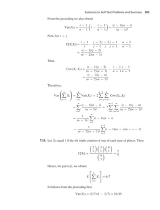
exchange of letters not only led to a complete solution to the problem of the points,

101. 86 Chapter 3 Conditional Probability and Independence
but also laid the framework for the solution to many other problems connected with
games of chance. This celebrated correspondence, dated by some as the birth date
of probability theory, was also important in stimulating interest in probability among
the mathematicians in Europe, for Pascal and Fermat were both recognized as being
among the foremost mathematicians of the time. For instance, within a short time of
their correspondence, the young Dutch mathematician Christiaan Huygens came to
Paris to discuss these problems and solutions, and interest and activity in this new
field grew rapidly.
EXAMPLE 4j The problem of the points
Independent trials resulting in a success with probability p and a failure with proba-
bility 1 − p are performed. What is the probability that n successes occur before m
failures? If we think of A and B as playing a game such that A gains 1 point when a
success occurs and B gains 1 point when a failure occurs, then the desired probability
is the probability that A would win if the game were to be continued in a position
where A needed n and B needed m more points to win.
Solution. We shall present two solutions. The first is due to Pascal and the second to
Fermat.
Let us denote by Pn,m the probability that n successes occur before m failures. By
conditioning on the outcome of the first trial, we obtain
Pn,m = pPn−1,m + (1 − p)Pn,m−1 n Ú 1, m Ú 1
(Why? Reason it out.) Using the obvious boundary conditions Pn, 0 = 0, P0, m = 1, we
can solve these equations for Pn,m. Rather than go through the tedious details, let us
instead consider Fermat’s solution.
Fermat argued that, in order for n successes to occur before m failures, it is nec-
essary and sufficient that there be at least n successes in the first m + n − 1 trials.
(Even if the game were to end before a total of m + n − 1 trials were completed, we
could still imagine that the necessary additional trials were performed.) This is true,
for if there are at least n successes in the first m + n − 1 trials, there could be at
most m − 1 failures in those m + n − 1 trials; thus, n successes would occur before
m failures. If, however, there were fewer than n successes in the first m + n − 1
trials, there would have to be at least m failures in that same number of trials; thus, n
successes would not occur before m failures.
Hence, since, as shown in Example 4f, the probability of exactly k successes in
m + n − 1 trials is
m + n − 1
k
pk(1 − p)m+n−1−k, it follows that the desired
probability of n successes before m failures is
Pn,m =
m+n−1
k=n
m + n − 1
k
pk
(1 − p)m+n−1−k
.
Our next two examples deal with gambling problems, with the first having a sur-
prisingly elegant analysis.∗
EXAMPLE 4k
Suppose that initially there are r players, with player i having ni units, ni 0, i =
1, ... , r. At each stage, two of the players are chosen to play a game, with the winner
∗The remainder of this section should be considered optional.

102. Section 3.4 Independent Events 87
of the game receiving 1 unit from the loser. Any player whose fortune drops to 0 is
eliminated, and this continues until a single player has all n K r
i=1 ni units, with
that player designated as the victor. Assuming that the results of successive games
are independent and that each game is equally likely to be won by either of its two
players, find Pi, the probability that player i is the victor?
Solution. To begin, suppose that there are n players, with each player initially having
1 unit. Consider player i. Each stage she plays will be equally likely to result in her
either winning or losing 1 unit, with the results from each stage being independent.
In addition, she will continue to play stages until her fortune becomes either 0 or n.
Because this is the same for all n players, it follows that each player has the same
chance of being the victor, implying that each player has probability 1/n of being the
victor. Now, suppose these n players are divided into r teams, with team i containing
ni players, i = 1, ... , r. Then the probability that the victor is a member of team i is
ni/n. But because
(a) team i initially has a total fortune of ni units, i = 1, ... , r, and
(b) each game played by members of different teams is equally likely to be won by
either player and results in the fortune of members of the winning team increas-
ing by 1 and the fortune of the members of the losing team decreasing by 1,
it is easy to see that the probability that the victor is from team i is exactly the prob-
ability we desire. Thus, Pi = ni/n. Interestingly, our argument shows that this result
does not depend on how the players in each stage are chosen. .
In the gambler’s ruin problem, there are only 2 gamblers, but they are not assumed
to be of equal skill.
EXAMPLE 4l The gambler’s ruin problem
Two gamblers, A and B, bet on the outcomes of successive flips of a coin. On each
flip, if the coin comes up heads, A collects 1 unit from B, whereas if it comes up tails,
A pays 1 unit to B. They continue to do this until one of them runs out of money. If
it is assumed that the successive flips of the coin are independent and each flip results
in a head with probability p, what is the probability that A ends up with all the money
if he starts with i units and B starts with N − i units?
Solution. Let E denote the event that A ends up with all the money when he starts
with i and B starts with N − i, and to make clear the dependence on the initial fortune
of A, let Pi = P(E). We shall obtain an expression for P(E) by conditioning on the
outcome of the first flip as follows: Let H denote the event that the first flip lands on
heads; then
Pi = P(E) = P(E|H)P(H) + P(E|Hc
)P(Hc
)
= pP(E|H) + (1 − p)P(E|Hc
)
Now, given that the first flip lands on heads, the situation after the first bet is that
A has i + 1 units and B has N − (i + 1). Since the successive flips are assumed to
be independent with a common probability p of heads, it follows that, from that point
on, A’s probability of winning all the money is exactly the same as if the game were
just starting with A having an initial fortune of i + 1 and B having an initial fortune
of N − (i + 1). Therefore,
P(E|H) = Pi+1

103. 88 Chapter 3 Conditional Probability and Independence
and similarly,
P(E|Hc
) = Pi−1
Hence, letting q = 1 − p, we obtain
Pi = pPi+1 + qPi−1 i = 1, 2, ... , N − 1 (4.2)
By making use of the obvious boundary conditions P0 = 0 and PN = 1, we shall
now solve Equation (4.2). Since p + q = 1, these equations are equivalent to
pPi + qPi = pPi+1 + qPi−1
or
Pi+1 − Pi =
q
p
(Pi − Pi−1) i = 1, 2, ... , N − 1 (4.3)
Hence, since P0 = 0, we obtain, from Equation (4.3),
P2 − P1 =
q
p
(P1 − P0) =
q
p
P1
P3 − P2 =
q
p
(P2 − P1) =
q
p
2
P1
.
.
. (4.4)
Pi − Pi−1 =
q
p
(Pi−1 − Pi−2) =
q
p
i−1
P1
.
.
.
PN − PN−1 =
q
p
(PN−1 − PN−2) =
q
p
N−1
P1
Adding the first i − 1 equations of (4.4) yields
Pi − P1 = P1
q
p
+
q
p
2
+ · · · +
q
p
i−1
or
Pi =
⎧
⎪
⎪
⎪
⎨
⎪
⎪
⎪
⎩
1 − (q/p)i
1 − (q/p)
P1 if
q
p
Z 1
iP1 if
q
p
= 1
Using the fact that PN = 1, we obtain
P1 =
⎧
⎪
⎪
⎨
⎪
⎪
⎩
1 − (q/p)
1 − (q/p)N
if p Z 1
2
1
N
if p = 1
2

104. Section 3.4 Independent Events 89
Hence,
Pi =
⎧
⎪
⎪
⎨
⎪
⎪
⎩
1 − (q/p)i
1 − (q/p)N
if p Z 1
2
i
N if p = 1
2
(4.5)
Let Qi denote the probability that B winds up with all the money when A starts
with i and B starts with N − i. Then, by symmetry to the situation described, and on
replacing p by q and i by N − i, it follows that
Qi =
⎧
⎪
⎪
⎪
⎨
⎪
⎪
⎪
⎩
1 − (p/q)N−i
1 − (p/q)N
if q Z 1
2
N − i
N
if q = 1
2
Moreover, since q = 1
2 is equivalent to p = 1
2, we have, when q Z 1
2,
Pi + Qi =
1 − (q/p)i
1 − (q/p)N
+
1 − (p/q)N−i
1 − (p/q)N
=
pN − pN(q/p)i
pN − qN
+
qN − qN(p/q)N−i
qN − pN
=
pN − pN−iqi − qN + qipN−i
pN − qN
= 1
This result also holds when p = q = 1
2, so
Pi + Qi = 1
In words, this equation states that, with probability 1, either A or B will wind up
with all of the money; in other words, the probability that the game continues indefi-
nitely with A’s fortune always being between 1 and N − 1 is zero. (The reader must
be careful because, a priori, there are three possible outcomes of this gambling game,
not two: Either A wins, or B wins, or the game goes on forever with nobody winning.
We have just shown that this last event has probability 0.)
As a numerical illustration of the preceding result, if A were to start with 5 units
and B with 10, then the probability of A’s winning would be 1
3 if p were 1
2 , whereas it
would jump to
1 −
2
3
5
1 −
2
3
15
L .87
if p were .6.
A special case of the gambler’s ruin problem, which is also known as the problem of
duration of play, was proposed to Huygens by Fermat in 1657. The version Huygens
proposed, which he himself solved, was that A and B have 12 coins each. They play
for these coins in a game with 3 dice as follows: Whenever 11 is thrown (by either—it
makes no difference who rolls the dice), A gives a coin to B. Whenever 14 is thrown,
B gives a coin to A. The person who first wins all the coins wins the game. Since

105. 90 Chapter 3 Conditional Probability and Independence
P{roll 11} = 27
216 and P{roll 14} = 15
216, we see from Example 4h that, for A, this is
just the gambler’s ruin problem with p = 15
42, i = 12, and N = 24. The general form
of the gambler’s ruin problem was solved by the mathematician James Bernoulli and
published 8 years after his death in 1713.
For an application of the gambler’s ruin problem to drug testing, suppose that two
new drugs have been developed for treating a certain disease. Drug i has a cure rate
Pi, i = 1, 2, in the sense that each patient treated with drug i will be cured with proba-
bility Pi. These cure rates are, however, not known, and we are interested in finding a
method for deciding whether P1 P2 or P2 P1. To decide on one of these alterna-
tives, consider the following test: Pairs of patients are to be treated sequentially, with
one member of the pair receiving drug 1 and the other drug 2. The results for each
pair are determined, and the testing stops when the cumulative number of cures from
one of the drugs exceeds the cumulative number of cures from the other by some
fixed, predetermined number. More formally, let
Xj =
%
1 if the patient in the jth pair that receives drug 1 is cured
0 otherwise
Yj =
%
1 if the patient in the jth pair that receives drug 2 is cured
0 otherwise
For a predetermined positive integer M, the test stops after pair N, where N is the
first value of n such that either
X1 + · · · + Xn − (Y1 + · · · + Yn) = M
or
X1 + · · · + Xn − (Y1 + · · · + Yn) = −M
In the former case, we assert that P1 P2 and in the latter that P2 P1.
In order to help ascertain whether the foregoing is a good test, one thing we would
like to know is the probability that it leads to an incorrect decision. That is, for given
P1 and P2, where P1 P2, what is the probability that the test will incorrectly assert
that P2 P1? To determine this probability, note that after each pair is checked,
the cumulative difference of cures using drug 1 versus drug 2 will go up by 1 with
probability P1(1 − P2)—since this is the probability that drug 1 leads to a cure and
drug 2 does not—or go down by 1 with probability (1 − P1)P2, or remain the same
with probability P1P2 + (1 − P1)(1 − P2). Hence, if we consider only those pairs
in which the cumulative difference changes, then the difference will go up by 1 with
probability
P = P{up 1|up 1 or down 1}
=
P1(1 − P2)
P1(1 − P2) + (1 − P1)P2
and down by 1 with probability
1 − P =
P2(1 − P1)
P1(1 − P2) + (1 − P1)P2
Thus, the probability that the test will assert that P2 P1 is equal to the probability
that a gambler who wins each (one-unit) bet with probability P will go down M before
going up M. But Equation (4.5), with i = M, N = 2M, shows that this probability is
given by

106. Section 3.4 Independent Events 91
P{test asserts that P2 P1}
= 1 −
1 −
1 − P
P
M
1 −
1 − P
P
2M
= 1 −
1
1 +
1 − P
P
M
=
1
1 + γ M
where
γ =
P
1 − P
=
P1(1 − P2)
P2(1 − P1)
For instance, if P1 = .6 and P2 = .4, then the probability of an incorrect decision is
.017 when M = 5 and reduces to .0003 when M = 10. .
Suppose that we are presented with a set of elements and we want to determine
whether at least one member of the set has a certain property. We can attack this
question probabilistically by randomly choosing an element of the set in such a way
that each element has a positive probability of being selected. Then the original ques-
tion can be answered by a consideration of the probability that the randomly selected
element does not have the property of interest. If this probability is equal to 1, then
none of the elements of the set have the property; if it is less than 1, then at least one
element of the set has the property.
The final example of this section illustrates this technique.
EXAMPLE 4m
The complete graph having n vertices is defined to be a set of n points (called vertices)
in the plane and the
n
2
lines (called edges) connecting each pair of vertices. The
complete graph having 3 vertices is shown in Figure 3.3. Suppose now that each edge
in a complete graph having n vertices is to be colored either red or blue. For a fixed
integer k, a question of interest is, Is there a way of coloring the edges so that no set
of k vertices has all of its
k
2
connecting edges the same color? It can be shown by
a probabilistic argument that if n is not too large, then the answer is yes.
FIGURE 3.3

107. 92 Chapter 3 Conditional Probability and Independence
The argument runs as follows: Suppose that each edge is, independently, equally
likely to be colored either red or blue. That is, each edge is red with probability 1
2 .
Number the
n
k
sets of k vertices and define the events Ei, i = 1, ... ,
n
k
as
follows:
Ei = {all of the connecting edges of the ith set
of k vertices are the same color}
Now, since each of the
k
2
connecting edges of a set of k vertices is equally likely to
be either red or blue, it follows that the probability that they are all the same color is
P(Ei) = 2
1
2
k(k−1)/2
Therefore, because
P
⎛
⎝
i
Ei
⎞
⎠ …
i
P(Ei) (Boole’s inequality)
we find that P
i
Ei
, the probability that there is a set of k vertices all of whose
connecting edges are similarly colored, satisfies
P
⎛
⎝
i
Ei
⎞
⎠ …
n
k
1
2
k(k−1)/2−1
Hence, if
n
k
1
2
k(k−1)/2−1
1
or, equivalently, if
n
k
2k(k−1)/2−1
then the probability that at least one of the
n
k
sets of k vertices has all of its
connecting edges the same color is less than 1. Consequently, under the preceding
condition on n and k, it follows that there is a positive probability that no set of k
vertices has all of its connecting edges the same color. But this conclusion implies
that there is at least one way of coloring the edges for which no set of k vertices has
all of its connecting edges the same color. .
Remarks. (a) Whereas the preceding argument established a condition on n and
k that guarantees the existence of a coloring scheme satisfying the desired property,
it gives no information about how to obtain such a scheme (although one possibility
would be simply to choose the colors at random, check to see if the resulting coloring
satisfies the property, and repeat the procedure until it does).

108. Section 3.5 P(·|F ) Is a Probability 93
(b) The method of introducing probability into a problem whose statement is
purely deterministic has been called the probabilistic method.† Other examples of this
method are given in Theoretical Exercise 24 and Examples 2t and 2u of Chapter 7.
3.5 P(·|F) IS A PROBABILITY
Conditional probabilities satisfy all of the properties of ordinary probabilities, as is
proved by Proposition 5.1, which shows that P(E|F) satisfies the three axioms of a
probability.
Proposition 5.1.
(a) 0 … P(E|F) … 1.
(b) P(S|F) = 1.
(c) If Ei, i = 1, 2, ..., are mutually exclusive events, then
P
⎛
⎝
q
1
Ei|F
⎞
⎠ =
q
1
P(Ei|F)
Proof. To prove part (a), we must show that 0 … P(EF)/P(F) … 1. The left-side
inequality is obvious, whereas the right side follows because EF ( F, which implies
that P(EF) … P(F). Part (b) follows because
P(S|F) =
P(SF)
P(F)
=
P(F)
P(F)
= 1
Part (c) follows from
P
⎛
⎝
q
i=1
Ei|F
⎞
⎠ =
P
⎛
⎝
q
i=1
Ei
F
⎞
⎠
P(F)
=
P
q
1
EiF
P(F)
since
⎛
⎝
q
1
Ei
⎞
⎠ F =
q
1
EiF
=
q
1
P(EiF)
P(F)
=
q
1
P(Ei|F)
where the next-to-last equality follows because EiEj = Ø implies that
EiFEjF = Ø.
†See N. Alon, J. Spencer, and P. Erdos, The Probabilistic Method (New York: John Wiley
Sons, Inc., 1992).

109. 94 Chapter 3 Conditional Probability and Independence
If we define Q(E) = P(E|F), then, from Proposition 5.1, Q(E) may be regarded
as a probability function on the events of S. Hence, all of the propositions previously
proved for probabilities apply to Q(E). For instance, we have
Q(E1 ∪ E2) = Q(E1) + Q(E2) − Q(E1E2)
or, equivalently,
P(E1 ∪ E2|F) = P(E1|F) + P(E2|F) − P(E1E2|F)
Also, if we define the conditional probability Q(E1|E2) by Q(E1|E2) = Q(E1E2)/
Q(E2), then, from Equation (3.1), we have
Q(E1) = Q(E1|E2)Q(E2) + Q(E1|Ec
2)Q(Ec
2) (5.1)
Since
Q(E1|E2) =
Q(E1E2)
Q(E2)
=
P(E1E2|F)
P(E2|F)
=
P(E1E2F)
P(F)
P(E2F)
P(F)
= P(E1|E2F)
Equation (5.1) is equivalent to
P(E1|F) = P(E1|E2F)P(E2|F) + P(E1|Ec
2F)P(Ec
2|F)
EXAMPLE 5a
Consider Example 3a, which is concerned with an insurance company which believes
that people can be divided into two distinct classes: those who are accident prone
and those who are not. During any given year, an accident-prone person will have an
accident with probability .4, whereas the corresponding figure for a person who is not
prone to accidents is .2. What is the conditional probability that a new policyholder
will have an accident in his or her second year of policy ownership, given that the
policyholder has had an accident in the first year?
Solution. If we let A be the event that the policyholder is accident prone and we let
Ai, i = 1, 2, be the event that he or she has had an accident in the ith year, then the
desired probability P(A2|A1) may be obtained by conditioning on whether or not the
policyholder is accident prone, as follows:
P(A2|A1) = P(A2|AA1)P(A|A1) + P(A2|Ac
A1)P(Ac
|A1)
Now,
P(A|A1) =
P(A1A)
P(A1)
=
P(A1|A)P(A)
P(A1)
However, P(A) is assumed to equal 3
10 , and it was shown in Example 3a that P(A1) =
.26. Hence,
P(A|A1) =
(.4)(.3)
.26
=
6
13

110. Section 3.5 P(·|F ) Is a Probability 95
Thus,
P(Ac
|A1) = 1 − P(A|A1) =
7
13
Since P(A2|AA1) = .4 and P(A2|AcA1) = .2, it follows that
P(A2|A1) = (.4)
6
13
+ (.2)
7
13
L .29
.
EXAMPLE 5b
A female chimp has given birth. It is not certain, however, which of two male chimps
is the father. Before any genetic analysis has been performed, it is felt that the
probability that male number 1 is the father is p and the probability that male number
2 is the father is 1 − p. DNA obtained from the mother, male number 1, and male
number 2 indicate that, on one specific location of the genome, the mother has the
gene pair (A, A), male number 1 has the gene pair (a, a), and male number 2 has the
gene pair (A, a). If a DNA test shows that the baby chimp has the gene pair (A, a),
what is the probability that male number 1 is the father?
Solution. Let all probabilities be conditional on the event that the mother has the
gene pair (A, A), male number 1 has the gene pair (a, a), and male number 2 has
the gene pair (A, a). Now, let Mi be the event that male number i, i = 1, 2, is the
father, and let BA,a be the event that the baby chimp has the gene pair (A, a). Then
P(M1|BA,a) is obtained as follows:
P(M1|BA,a) =
P(M1BA,a)
P(BA,a)
=
P(BA,a|M1)P(M1)
P(BA,a|M1)P(M1) + P(BA,a|M2)P(M2)
=
1 · p
1 · p + (1/2)(1 − p)
=
2p
1 + p
Because 2p
1+p p when p 1, the information that the baby’s gene pair is (A, a)
increases the probability that male number 1 is the father. This result is intuitive
because it is more likely that the baby would have gene pair (A, a) if M1 is true than
if M2 is true (the respective conditional probabilities being 1 and 1/2). .
The next example deals with a problem in the theory of runs.
EXAMPLE 5c
Independent trials, each resulting in a success with probability p or a failure with
probability q = 1 − p, are performed. We are interested in computing the probability
that a run of n consecutive successes occurs before a run of m consecutive failures.
Solution. Let E be the event that a run of n consecutive successes occurs before a run
of m consecutive failures. To obtain P(E), we start by conditioning on the outcome of
the first trial. That is, letting H denote the event that the first trial results in a success,
we obtain
P(E) = pP(E|H) + qP(E|Hc
) (5.2)

111. 96 Chapter 3 Conditional Probability and Independence
Now, given that the first trial was successful, one way we can get a run of n successes
before a run of m failures would be to have the next n − 1 trials all result in successes.
So, let us condition on whether or not that occurs. That is, letting F be the event that
trials 2 through n all are successes, we obtain
P(E|H) = P(E|FH)P(F|H) + P(E|Fc
H)P(Fc
|H) (5.3)
On the one hand, clearly, P(E|FH) = 1; on the other hand, if the event FcH occurs,
then the first trial would result in a success, but there would be a failure some time
during the next n − 1 trials. However, when this failure occurs, it would wipe out all
of the previous successes, and the situation would be exactly as if we started out with
a failure. Hence,
P(E|Fc
H) = P(E|Hc
)
Because the independence of trials implies that F and H are independent, and because
P(F) = pn−1, it follows from Equation (5.3) that
P(E|H) = pn−1
+ (1 − pn−1
)P(E|Hc
) (5.4)
We now obtain an expression for P(E|Hc) in a similar manner. That is, we let G
denote the event that trials 2 through m are all failures. Then
P(E|Hc
) = P(E|GHc
)P(G|Hc
) + P(E|Gc
Hc
)P(Gc
|Hc
) (5.5)
Now, GHc is the event that the first m trials all result in failures, so P(E|GHc) = 0.
Also, if GcHc occurs, then the first trial is a failure, but there is at least one success
in the next m − 1 trials. Hence, since this success wipes out all previous failures, we
see that
P(E|Gc
Hc
) = P(E|H)
Thus, because P(Gc|Hc) = P(Gc) = 1 − qm−1, we obtain, from (5.5),
P(E|Hc
) = (1 − qm−1
)P(E|H) (5.6)
Solving Equations (5.4) and (5.6) yields
P(E|H) =
pn−1
pn−1 + qm−1 − pn−1qm−1
and
P(E|Hc
) =
(1 − qm−1)pn−1
pn−1 + qm−1 − pn−1qm−1
Thus,
P(E) = pP(E|H) + qP(E|Hc
)
=
pn + qpn−1(1 − qm−1)
pn−1 + qm−1 − pn−1qm−1
=
pn−1(1 − qm)
pn−1 + qm−1 − pn−1qm−1
(5.7)

112. Section 3.5 P(·|F ) Is a Probability 97
It is interesting to note that, by the symmetry of the problem, the probability of
obtaining a run of m failures before a run of n successes would be given by Equa-
tion (5.7) with p and q interchanged and n and m interchanged. Hence, this probabil-
ity would equal
P{run of m failures before a run of n successes}
=
qm−1(1 − pn)
qm−1 + pn−1 − qm−1pn−1
(5.8)
Since Equations (5.7) and (5.8) sum to 1, it follows that, with probability 1, either a
run of n successes or a run of m failures will eventually occur.
As an example of Equation (5.7), we note that, in tossing a fair coin, the probability
that a run of 2 heads will precede a run of 3 tails is 7
10. For 2 consecutive heads before
4 consecutive tails, the probability rises to 5
6 . .
In our next example, we return to the matching problem (Example 5m, Chapter 2)
and this time obtain a solution by using conditional probabilities.
EXAMPLE 5d
At a party, n men take off their hats. The hats are then mixed up, and each man
randomly selects one. We say that a match occurs if a man selects his own hat. What
is the probability of
(a) no matches?
(b) exactly k matches?
Solution. (a) Let E denote the event that no matches occur, and to make explicit the
dependence on n, write Pn = P(E). We start by conditioning on whether or not the
first man selects his own hat—call these events M and Mc, respectively. Then
Pn = P(E) = P(E|M)P(M) + P(E|Mc
)P(Mc
)
Clearly, P(E|M) = 0, so
Pn = P(E|Mc
)
n − 1
n
(5.9)
Now, P(E|Mc) is the probability of no matches when n − 1 men select from a set of
n − 1 hats that does not contain the hat of one of these men. This can happen in either
of two mutually exclusive ways: Either there are no matches and the extra man does
not select the extra hat (this being the hat of the man who chose first), or there are
no matches and the extra man does select the extra hat. The probability of the first of
these events is just Pn−1, which is seen by regarding the extra hat as “belonging” to
the extra man. Because the second event has probability [1/(n − 1)]Pn−2, we have
P(E|Mc
) = Pn−1 +
1
n − 1
Pn−2
Thus, from Equation (5.9),
Pn =
n − 1
n
Pn−1 +
1
n
Pn−2
or, equivalently,
Pn − Pn−1 = −
1
n
(Pn−1 − Pn−2) (5.10)

113. 98 Chapter 3 Conditional Probability and Independence
However, since Pn is the probability of no matches when n men select among their
own hats, we have
P1 = 0 P2 =
1
2
So, from Equation (5.10),
P3 − P2 = −
(P2 − P1)
3
= −
1
3!
or P3 =
1
2!
−
1
3!
P4 − P3 = −
(P3 − P2)
4
=
1
4!
or P4 =
1
2!
−
1
3!
+
1
4!
and, in general,
Pn =
1
2!
−
1
3!
+
1
4!
− · · · +
(−1)n
n!
(b) To obtain the probability of exactly k matches, we consider any fixed group of
k men. The probability that they, and only they, select their own hats is
1
n
1
n − 1
· · ·
1
n − (k − 1)
Pn−k =
(n − k)!
n!
Pn−k
where Pn−k is the conditional probability that the other n − k men, selecting among
their own hats, have no matches. Since there are
n
k
choices of a set of k men, the
desired probability of exactly k matches is
Pn−k
k!
=
1
2! − 1
3! + · · · +
(−1)n−k
(n − k)!
k!
.
An important concept in probability theory is that of the conditional independence
of events. We say that the events E1 and E2 are conditionally independent given F
if, given that F occurs, the conditional probability that E1 occurs is unchanged by
information as to whether or not E2 occurs. More formally, E1 and E2 are said to be
conditionally independent given F if
P(E1|E2F) = P(E1|F) (5.11)
or, equivalently,
P(E1E2|F) = P(E1|F)P(E2|F) (5.12)
The notion of conditional independence can easily be extended to more than two
events, and this extension is left as an exercise.
The reader should note that the concept of conditional independence was implic-
itly employed in Example 5a, where it was assumed that the events that a policyholder
had an accident in his or her ith year, i = 1, 2, ..., were conditionally independent
given whether or not the person was accident prone. The following example, some-
times referred to as Laplace’s rule of succession, further illustrates the concept of
conditional independence.
EXAMPLE 5e Laplace’s rule of succession
There are k + 1 coins in a box. When flipped, the ith coin will turn up heads with
probability i/k, i = 0, 1, ... , k. A coin is randomly selected from the box and is then

114. Section 3.5 P(·|F ) Is a Probability 99
repeatedly flipped. If the first n flips all result in heads, what is the conditional prob-
ability that the (n + 1)st flip will do likewise?
Solution. Let Ci denote the event that the ith coin, i = 0, 1, ... , k, is initially selected;
let Fn denote the event that the first n flips all result in heads; and let H be the event
that the (n + 1)st flip is a head. The desired probability, P(H|Fn), is now obtained as
follows:
P(H|Fn) =
k
i=0
P(H|FnCi)P(Ci|Fn)
Now, given that the ith coin is selected, it is reasonable to assume that the outcomes
will be conditionally independent, with each one resulting in a head with probability
i/k. Hence,
P(H|FnCi) = P(H|Ci) =
i
k
Also,
P(Ci|Fn) =
P(CiFn)
P(Fn)
=
P(Fn|Ci)P(Ci)
k
j=0
P(Fn|Cj)P(Cj)
=
(i/k)n[1/(k + 1)]
k
j=0
(j/k)n
[1/(k + 1)]
Thus,
P(H|Fn) =
k
i=0
(i/k)n+1
k
j=0
(j/k)n
But if k is large, we can use the integral approximations
1
k
k
i=0
i
k
n+1
L
* 1
0
xn+1
dx =
1
n + 2
1
k
k
j=0
j
k
n
L
* 1
0
xn
dx =
1
n + 1
So, for k large,
P(H|Fn) L
n + 1
n + 2 .
EXAMPLE 5f Updating information sequentially
Suppose there are n mutually exclusive and exhaustive possible hypotheses, with ini-
tial (sometimes referred to as prior) probabilities P(Hi), n
i=1 P(Hi) = 1. Now, if
information that the event E has occurred is received, then the conditional probabil-
ity that Hi is the true hypothesis (sometimes referred to as the updated or posterior
probability of Hi) is
P(Hi|E) =
P(E|Hi)P(Hi)
j P(E|Hj)P(Hj)
(5.13)

115. 100 Chapter 3 Conditional Probability and Independence
Suppose now that we learn first that E1 has occurred and then that E2 has occurred.
Then, given only the first piece of information, the conditional probability that Hi is
the true hypothesis is
P(Hi|E1) =
P(E1|Hi)P(Hi)
P(E1)
=
P(E1|Hi)P(Hi)
j P(E1|Hj)P(Hj)
whereas given both pieces of information, the conditional probability that Hi is the
true hypothesis is P(Hi|E1E2), which can be computed by
P(Hi|E1E2) =
P(E1E2|Hi)P(Hi)
j P(E1E2|Hj)P(Hj)
One might wonder, however, when one can compute P(Hi|E1E2) by using the
right side of Equation (5.13) with E = E2 and with P(Hj) replaced by P(Hj|E1),
j = 1, ... , n. That is, when is it legitimate to regard P(Hj|E1), j Ú 1, as the prior
probabilities and then use (5.13) to compute the posterior probabilities?
Solution. The answer is that the preceding is legitimate, provided that, for each j =
1, ... , n, the events E1 and E2 are conditionally independent, given Hj. For if this is
the case, then
P(E1E2|Hj) = P(E2|Hj)P(E1|Hj), j = 1, ... , n
Therefore,
P(Hi|E1E2) =
P(E2|Hi)P(E1|Hi)P(Hi)
P(E1E2)
=
P(E2|Hi)P(E1Hi)
P(E1E2)
=
P(E2|Hi)P(Hi|E1)P(E1)
P(E1E2)
=
P(E2|Hi)P(Hi|E1)
Q(1, 2)
where Q(1, 2) = P(E1E2)
P(E1) . Since the preceding equation is valid for all i, we obtain,
upon summing,
1 =
n
i=1
P(Hi|E1E2) =
n
i=1
P(E2|Hi)P(Hi|E1)
Q(1, 2)
showing that
Q(1, 2) =
n
i=1
P(E2|Hi)P(Hi|E1)
and yielding the result
P(Hi|E1E2) =
P(E2|Hi)P(Hi|E1)
n
i=1 P(E2|Hi)P(Hi|E1)
For instance, suppose that one of two coins is chosen to be flipped. Let Hi be the event
that coin i, i = 1, 2, is chosen, and suppose that when coin i is flipped, it lands on heads
with probability pi, i = 1, 2. Then the preceding equations show that, to sequentially

116. Summary 101
update the probability that coin 1 is the one being flipped, given the results of the
previous flips, all that must be saved after each new flip is the conditional probability
that coin 1 is the coin being used. That is, it is not necessary to keep track of all earlier
results. .
SUMMARY
For events E and F, the conditional probability of E given that F has occurred is
denoted by P(E|F) and is defined by
P(E|F) =
P(EF)
P(F)
The identity
P(E1E2 · · · En) = P(E1)P(E2|E1) · · · P(En|E1 · · · En−1)
is known as the multiplication rule of probability.
A valuable identity is
P(E) = P(E|F)P(F) + P(E|Fc
)P(Fc
)
which can be used to compute P(E) by “conditioning” on whether F occurs.
P(H)/P(Hc) is called the odds of the event H. The identity
P(H|E)
P(Hc|E)
=
P(H) P(E|H)
P(Hc)P(E|Hc)
shows that when new evidence E is obtained, the value of the odds of H becomes its
old value multiplied by the ratio of the conditional probability of the new evidence
when H is true to the conditional probability when H is not true.
Let Fi, i = 1, ... , n, be mutually exclusive events whose union is the entire sample
space. The identity
P(Fj|E) =
P(E|Fj)P(Fj)
n
i=1
P(E|Fi)P(Fi)
is known as Bayes’s formula. If the events Fi, i = 1, ... , n, are competing hypotheses,
then Bayes’s formula shows how to compute the conditional probabilities of these
hypotheses when additional evidence E becomes available.
If P(EF) = P(E)P(F), then we say that the events E and F are independent. This
condition is equivalent to P(E|F) = P(E) and to P(F|E) = P(F). Thus, the events E
and F are independent if knowledge of the occurrence of one of them does not affect
the probability of the other.
The events E1, ... , En are said to be independent if, for any subset Ei1
, ... , Eir
of them,
P(Ei1
· · · Eir ) = P(Ei1
) · · · P(Eir )
For a fixed event F, P(E|F) can be considered to be a probability function on the
events E of the sample space.

117. 102 Chapter 3 Conditional Probability and Independence
PROBLEMS
3.1. Two fair dice are rolled. What is the conditional
probability that at least one lands on 6 given that
the dice land on different numbers?
3.2. If two fair dice are rolled, what is the conditional
probability that the first one lands on 6 given that
the sum of the dice is i? Compute for all values of
i between 2 and 12.
3.3. Use Equation (2.1) to compute, in a hand of
bridge, the conditional probability that East has
3 spades given that North and South have a com-
bined total of 8 spades.
3.4. What is the probability that at least one of a pair of
fair dice lands on 6, given that the sum of the dice
is i, i = 2, 3, ... , 12?
3.5. An urn contains 6 white and 9 black balls. If 4 balls
are to be randomly selected without replacement,
what is the probability that the first 2 selected are
white and the last 2 black?
3.6. Consider an urn containing 12 balls, of which 8
are white. A sample of size 4 is to be drawn with
replacement (without replacement). What is the
conditional probability (in each case) that the first
and third balls drawn will be white given that the
sample drawn contains exactly 3 white balls?
3.7. The king comes from a family of 2 children. What
is the probability that the other child is his sister?
3.8. A couple has 2 children. What is the probability
that both are girls if the older of the two is a girl?
3.9. Consider 3 urns. Urn A contains 2 white and 4 red
balls, urn B contains 8 white and 4 red balls, and
urn C contains 1 white and 3 red balls. If 1 ball is
selected from each urn, what is the probability that
the ball chosen from urn A was white given that
exactly 2 white balls were selected?
3.10. Three cards are randomly selected, without
replacement, from an ordinary deck of 52 playing
cards. Compute the conditional probability that
the first card selected is a spade given that the sec-
ond and third cards are spades.
3.11. Two cards are randomly chosen without replace-
ment from an ordinary deck of 52 cards. Let B be
the event that both cards are aces, let As be the
event that the ace of spades is chosen, and let A be
the event that at least one ace is chosen. Find
(a) P(B|As)
(b) P(B|A)
3.12. A recent college graduate is planning to take the
first three actuarial examinations in the coming
summer. She will take the first actuarial exam in
June. If she passes that exam, then she will take
the second exam in July, and if she also passes that
one, then she will take the third exam in Septem-
ber. If she fails an exam, then she is not allowed
to take any others. The probability that she passes
the first exam is .9. If she passes the first exam, then
the conditional probability that she passes the sec-
ond one is .8, and if she passes both the first and
the second exams, then the conditional probability
that she passes the third exam is .7.
(a) What is the probability that she passes all
three exams?
(b) Given that she did not pass all three exams,
what is the conditional probability that she
failed the second exam?
3.13. Suppose that an ordinary deck of 52 cards (which
contains 4 aces) is randomly divided into 4 hands
of 13 cards each. We are interested in determining
p, the probability that each hand has an ace. Let Ei
be the event that the ith hand has exactly one ace.
Determine p = P(E1E2E3E4) by using the multi-
plication rule.
3.14. An urn initially contains 5 white and 7 black balls.
Each time a ball is selected, its color is noted and
it is replaced in the urn along with 2 other balls of
the same color. Compute the probability that
(a) the first 2 balls selected are black and the next
2 are white;
(b) of the first 4 balls selected, exactly 2 are black.
3.15. An ectopic pregnancy is twice as likely to develop
when the pregnant woman is a smoker as it is when
she is a nonsmoker. If 32 percent of women of
childbearing age are smokers, what percentage of
women having ectopic pregnancies are smokers?
3.16. Ninety-eight percent of all babies survive delivery.
However, 15 percent of all births involve Cesarean
(C) sections, and when a C section is performed,
the baby survives 96 percent of the time. If a ran-
domly chosen pregnant woman does not have a
C section, what is the probability that her baby
survives?
3.17. In a certain community, 36 percent of the families
own a dog and 22 percent of the families that own
a dog also own a cat. In addition, 30 percent of the
families own a cat. What is
(a) the probability that a randomly selected fam-
ily owns both a dog and a cat?
(b) the conditional probability that a randomly
selected family owns a dog given that it owns
a cat?
3.18. A total of 46 percent of the voters in a certain city
classify themselves as Independents, whereas 30
percent classify themselves as Liberals and 24 per-
cent say that they are Conservatives. In a recent
local election, 35 percent of the Independents, 62
percent of the Liberals, and 58 percent of the Con-
servatives voted. A voter is chosen at random.

118. Problems 103
Given that this person voted in the local election,
what is the probability that he or she is
(a) an Independent?
(b) a Liberal?
(c) a Conservative?
(d) What fraction of voters participated in the
local election?
3.19. A total of 48 percent of the women and 37 percent
of the men that took a certain “quit smoking” class
remained nonsmokers for at least one year after
completing the class. These people then attended
a success party at the end of a year. If 62 percent
of the original class was male,
(a) what percentage of those attending the party
were women?
(b) what percentage of the original class attended
the party?
3.20. Fifty-two percent of the students at a certain col-
lege are females. Five percent of the students in
this college are majoring in computer science. Two
percent of the students are women majoring in
computer science. If a student is selected at ran-
dom, find the conditional probability that
(a) the student is female given that the student is
majoring in computer science;
(b) this student is majoring in computer science
given that the student is female.
3.21. A total of 500 married working couples were
polled about their annual salaries, with the follow-
ing information resulting:
Husband
Wife Less than More than
$25,000 $25,000
Less than $25,000 212 198
More than $25,000 36 54
For instance, in 36 of the couples, the wife earned
more and the husband earned less than $25,000. If
one of the couples is randomly chosen, what is
(a) the probability that the husband earns less
than $25,000?
(b) the conditional probability that the wife earns
more than $25,000 given that the husband
earns more than this amount?
(c) the conditional probability that the wife earns
more than $25,000 given that the husband
earns less than this amount?
3.22. A red die, a blue die, and a yellow die (all six
sided) are rolled. We are interested in the prob-
ability that the number appearing on the blue die
is less than that appearing on the yellow die, which
is less than that appearing on the red die. That is,
with B, Y, and R denoting, respectively, the num-
ber appearing on the blue, yellow, and red die, we
are interested in P(B Y R).
(a) What is the probability that no two of the dice
land on the same number?
(b) Given that no two of the dice land on the same
number, what is the conditional probability
that B Y R?
(c) What is P(B Y R)?
3.23. Urn I contains 2 white and 4 red balls, whereas urn
II contains 1 white and 1 red ball. A ball is ran-
domly chosen from urn I and put into urn II, and a
ball is then randomly selected from urn II. What is
(a) the probability that the ball selected from urn
II is white?
(b) the conditional probability that the trans-
ferred ball was white given that a white ball
is selected from urn II?
3.24. Each of 2 balls is painted either black or gold and
then placed in an urn. Suppose that each ball is col-
ored black with probability 1
2 and that these events
are independent.
(a) Suppose that you obtain information that the
gold paint has been used (and thus at least
one of the balls is painted gold). Compute
the conditional probability that both balls are
painted gold.
(b) Suppose now that the urn tips over and 1 ball
falls out. It is painted gold. What is the prob-
ability that both balls are gold in this case?
Explain.
3.25. The following method was proposed to estimate
the number of people over the age of 50 who reside
in a town of known population 100,000: “As you
walk along the streets, keep a running count of the
percentage of people you encounter who are over
50. Do this for a few days; then multiply the per-
centage you obtain by 100,000 to obtain the esti-
mate.” Comment on this method.
Hint: Let p denote the proportion of people in the
town who are over 50. Furthermore, let α1 denote
the proportion of time that a person under the age
of 50 spends in the streets, and let α2 be the cor-
responding value for those over 50. What quantity
does the method suggested estimate? When is the
estimate approximately equal to p?
3.26. Suppose that 5 percent of men and .25 percent
of women are color blind. A color-blind person
is chosen at random. What is the probability of
this person being male? Assume that there are an
equal number of males and females. What if the
population consisted of twice as many males as
females?
3.27. All the workers at a certain company drive to
work and park in the company’s lot. The company

119. 104 Chapter 3 Conditional Probability and Independence
is interested in estimating the average number of
workers in a car. Which of the following methods
will enable the company to estimate this quantity?
Explain your answer.
1. Randomly choose n workers, find out how
many were in the cars in which they were
driven, and take the average of the n values.
2. Randomly choose n cars in the lot, find out how
many were driven in those cars, and take the
average of the n values.
3.28. Suppose that an ordinary deck of 52 cards is shuf-
fled and the cards are then turned over one at a
time until the first ace appears. Given that the first
ace is the 20th card to appear, what is the condi-
tional probability that the card following it is the
(a) ace of spades?
(b) two of clubs?
3.29. There are 15 tennis balls in a box, of which 9 have
not previously been used. Three of the balls are
randomly chosen, played with, and then returned
to the box. Later, another 3 balls are randomly
chosen from the box. Find the probability that
none of these balls has ever been used.
3.30. Consider two boxes, one containing 1 black and 1
white marble, the other 2 black and 1 white mar-
ble. A box is selected at random, and a marble is
drawn from it at random. What is the probability
that the marble is black? What is the probability
that the first box was the one selected given that
the marble is white?
3.31. Ms. Aquina has just had a biopsy on a possibly can-
cerous tumor. Not wanting to spoil a weekend fam-
ily event, she does not want to hear any bad news
in the next few days. But if she tells the doctor to
call only if the news is good, then if the doctor does
not call, Ms. Aquina can conclude that the news is
bad. So, being a student of probability, Ms. Aquina
instructs the doctor to flip a coin. If it comes up
heads, the doctor is to call if the news is good and
not call if the news is bad. If the coin comes up
tails, the doctor is not to call. In this way, even if
the doctor doesn’t call, the news is not necessarily
bad. Let α be the probability that the tumor is can-
cerous; let β be the conditional probability that the
tumor is cancerous given that the doctor does not
call.
(a) Which should be larger, α or β?
(b) Find β in terms of α, and prove your answer
in part (a).
3.32. A family has j children with probability pj, where
p1 = .1, p2 = .25, p3 = .35, p4 = .3. A child
from this family is randomly chosen. Given that
this child is the eldest child in the family, find the
conditional probability that the family has
(a) only 1 child;
(b) 4 children.
Redo (a) and (b) when the randomly selected child
is the youngest child of the family.
3.33. On rainy days, Joe is late to work with probability
.3; on nonrainy days, he is late with probability .1.
With probability .7, it will rain tomorrow.
(a) Find the probability that Joe is early tomor-
row.
(b) Given that Joe was early, what is the condi-
tional probability that it rained?
3.34. In Example 3f, suppose that the new evidence is
subject to different possible interpretations and in
fact shows only that it is 90 percent likely that the
criminal possesses the characteristic in question. In
this case, how likely would it be that the suspect is
guilty (assuming, as before, that he has the charac-
teristic)?
3.35. With probability .6, the present was hidden by
mom; with probability .4, it was hidden by dad.
When mom hides the present, she hides it upstairs
70 percent of the time and downstairs 30 percent
of the time. Dad is equally likely to hide it upstairs
or downstairs.
(a) What is the probability that the present is
upstairs?
(b) Given that it is downstairs, what is the proba-
bility it was hidden by dad?
3.36. Stores A, B, and C have 50, 75, and 100 employees,
respectively, and 50, 60, and 70 percent of them
respectively are women. Resignations are equally
likely among all employees, regardless of sex. One
woman employee resigns. What is the probability
that she works in store C?
3.37. (a) A gambler has a fair coin and a two-headed
coin in his pocket. He selects one of the coins
at random; when he flips it, it shows heads.
What is the probability that it is the fair coin?
(b) Suppose that he flips the same coin a second
time and, again, it shows heads. Now what is
the probability that it is the fair coin?
(c) Suppose that he flips the same coin a third
time and it shows tails. Now what is the prob-
ability that it is the fair coin?
3.38. Urn A has 5 white and 7 black balls. Urn B has
3 white and 12 black balls. We flip a fair coin. If
the outcome is heads, then a ball from urn A is
selected, whereas if the outcome is tails, then a ball
from urn B is selected. Suppose that a white ball
is selected. What is the probability that the coin
landed tails?
3.39. In Example 3a, what is the probability that some-
one has an accident in the second year given that
he or she had no accidents in the first year?
3.40. Consider a sample of size 3 drawn in the following
manner: We start with an urn containing 5 white

120. Problems 105
and 7 red balls. At each stage, a ball is drawn
and its color is noted. The ball is then returned
to the urn, along with an additional ball of the
same color. Find the probability that the sample
will contain exactly
(a) 0 white balls;
(b) 1 white ball;
(c) 3 white balls;
(d) 2 white balls.
3.41. A deck of cards is shuffled and then divided into
two halves of 26 cards each. A card is drawn from
one of the halves; it turns out to be an ace. The ace
is then placed in the second half-deck. The half is
then shuffled, and a card is drawn from it. Com-
pute the probability that this drawn card is an ace.
Hint: Condition on whether or not the inter-
changed card is selected.
3.42. Three cooks, A, B, and C, bake a special kind of
cake, and with respective probabilities .02, .03, and
.05, it fails to rise. In the restaurant where they
work, A bakes 50 percent of these cakes, B 30 per-
cent, and C 20 percent. What proportion of “fail-
ures” is caused by A?
3.43. There are 3 coins in a box. One is a two-headed
coin, another is a fair coin, and the third is a biased
coin that comes up heads 75 percent of the time.
When one of the 3 coins is selected at random and
flipped, it shows heads. What is the probability that
it was the two-headed coin?
3.44. Three prisoners are informed by their jailer that
one of them has been chosen at random to be
executed and the other two are to be freed. Pris-
oner A asks the jailer to tell him privately which of
his fellow prisoners will be set free, claiming that
there would be no harm in divulging this informa-
tion because he already knows that at least one of
the two will go free. The jailer refuses to answer
the question, pointing out that if A knew which
of his fellow prisoners were to be set free, then
his own probability of being executed would rise
from 1
3 to 1
2 because he would then be one of two
prisoners. What do you think of the jailer’s
reasoning?
3.45. Suppose we have 10 coins such that if the ith
coin is flipped, heads will appear with probabil-
ity i/10, i = 1, 2, ... , 10. When one of the coins
is randomly selected and flipped, it shows heads.
What is the conditional probability that it was the
fifth coin?
3.46. In any given year, a male automobile policyholder
will make a claim with probability pm and a female
policyholder will make a claim with probability pf ,
where pf Z pm. The fraction of the policyholders
that are male is α, 0 α 1. A policyholder is
randomly chosen. If Ai denotes the event that this
policyholder will make a claim in year i, show that
P(A2|A1) P(A1)
Give an intuitive explanation of why the preceding
inequality is true.
3.47. An urn contains 5 white and 10 black balls. A fair
die is rolled and that number of balls is randomly
chosen from the urn. What is the probability that
all of the balls selected are white? What is the con-
ditional probability that the die landed on 3 if all
the balls selected are white?
3.48. Each of 2 cabinets identical in appearance has 2
drawers. Cabinet A contains a silver coin in each
drawer, and cabinet B contains a silver coin in
one of its drawers and a gold coin in the other.
A cabinet is randomly selected, one of its drawers
is opened, and a silver coin is found. What is the
probability that there is a silver coin in the other
drawer?
3.49. Prostate cancer is the most common type of can-
cer found in males. As an indicator of whether a
male has prostate cancer, doctors often perform
a test that measures the level of the prostate-
specific antigen (PSA) that is produced only by the
prostate gland. Although PSA levels are indica-
tive of cancer, the test is notoriously unreli-
able. Indeed, the probability that a noncancerous
man will have an elevated PSA level is approx-
imately .135, increasing to approximately .268 if
the man does have cancer. If, on the basis of other
factors, a physician is 70 percent certain that a
male has prostate cancer, what is the conditional
probability that he has the cancer given that
(a) the test indicated an elevated PSA level?
(b) the test did not indicate an elevated PSA
level?
Repeat the preceding calculation, this time assum-
ing that the physician initially believes that there
is a 30 percent chance that the man has prostate
cancer.
3.50. Suppose that an insurance company classifies peo-
ple into one of three classes: good risks, average
risks, and bad risks. The company’s records indi-
cate that the probabilities that good-, average-, and
bad-risk persons will be involved in an accident
over a 1-year span are, respectively, .05, .15, and
.30. If 20 percent of the population is a good risk,
50 percent an average risk, and 30 percent a bad
risk, what proportion of people have accidents in
a fixed year? If policyholder A had no accidents
in 1997, what is the probability that he or she is a
good or average risk?
3.51. A worker has asked her supervisor for a letter of
recommendation for a new job. She estimates that
there is an 80 percent chance that she will get the

121. 106 Chapter 3 Conditional Probability and Independence
job if she receives a strong recommendation, a 40
percent chance if she receives a moderately good
recommendation, and a 10 percent chance if she
receives a weak recommendation. She further esti-
mates that the probabilities that the recommenda-
tion will be strong, moderate, and weak are .7, .2,
and .1, respectively.
(a) How certain is she that she will receive the
new job offer?
(b) Given that she does receive the offer, how
likely should she feel that she received a
strong recommendation? a moderate recom-
mendation? a weak recommendation?
(c) Given that she does not receive the job offer,
how likely should she feel that she received a
strong recommendation? a moderate recom-
mendation? a weak recommendation?
3.52. A high school student is anxiously waiting to
receive mail telling her whether she has been
accepted to a certain college. She estimates that
the conditional probabilities of receiving notifica-
tion on each day of next week, given that she is
accepted and that she is rejected, are as follows:
Day P(mail|accepted) P(mail|rejected)
Monday .15 .05
Tuesday .20 .10
Wednesday .25 .10
Thursday .15 .15
Friday .10 .20
She estimates that her probability of being
accepted is .6.
(a) What is the probability that she receives mail
on Monday?
(b) What is the conditional probability that she
received mail on Tuesday given that she does
not receive mail on Monday?
(c) If there is no mail through Wednesday, what
is the conditional probability that she will be
accepted?
(d) What is the conditional probability that she
will be accepted if mail comes on Thursday?
(e) What is the conditional probability that she
will be accepted if no mail arrives that week?
3.53. A parallel system functions whenever at least one
of its components works. Consider a parallel sys-
tem of n components, and suppose that each com-
ponent works independently with probability 1
2 .
Find the conditional probability that component 1
works given that the system is functioning.
3.54. If you had to construct a mathematical model for
events E and F, as described in parts (a) through
(e), would you assume that they were independent
events? Explain your reasoning.
(a) E is the event that a businesswoman has blue
eyes, and F is the event that her secretary has
blue eyes.
(b) E is the event that a professor owns a car,
and F is the event that he is listed in the tele-
phone book.
(c) E is the event that a man is under 6 feet tall,
and F is the event that he weighs over 200
pounds.
(d) E is the event that a woman lives in the United
States, and F is the event that she lives in the
Western Hemisphere.
(e) E is the event that it will rain tomorrow, and
F is the event that it will rain the day after
tomorrow.
3.55. In a class, there are 4 freshman boys, 6 freshman
girls, and 6 sophomore boys. How many sopho-
more girls must be present if sex and class are to
be independent when a student is selected at ran-
dom?
3.56. Suppose that you continually collect coupons and
that there are m different types. Suppose also that
each time a new coupon is obtained, it is a type
i coupon with probability pi, i = 1, ... , m. Suppose
that you have just collected your nth coupon. What
is the probability that it is a new type?
Hint: Condition on the type of this coupon.
3.57. A simplified model for the movement of the price
of a stock supposes that on each day the stock’s
price either moves up 1 unit with probability p or
moves down 1 unit with probability 1 − p. The
changes on different days are assumed to be inde-
pendent.
(a) What is the probability that after 2 days the
stock will be at its original price?
(b) What is the probability that after 3 days the
stock’s price will have increased by 1 unit?
(c) Given that after 3 days the stock’s price has
increased by 1 unit, what is the probability
that it went up on the first day?
3.58. Suppose that we want to generate the outcome
of the flip of a fair coin, but that all we have at
our disposal is a biased coin which lands on heads
with some unknown probability p that need not be
equal to 1
2 . Consider the following procedure for
accomplishing our task:
1. Flip the coin.
2. Flip the coin again.
3. If both flips land on heads or both land on tails,
return to step 1.
4. Let the result of the last flip be the result of the
experiment.

122. Problems 107
(a) Show that the result is equally likely to be
either heads or tails.
(b) Could we use a simpler procedure that contin-
ues to flip the coin until the last two flips are
different and then lets the result be the out-
come of the final flip?
3.59. Independent flips of a coin that lands on heads
with probability p are made. What is the proba-
bility that the first four outcomes are
(a) H, H, H, H?
(b) T, H, H, H?
(c) What is the probability that the pattern T, H,
H, H occurs before the pattern H, H, H, H?
Hint for part (c): How can the pattern H, H, H, H
occur first?
3.60. The color of a person’s eyes is determined by a sin-
gle pair of genes. If they are both blue-eyed genes,
then the person will have blue eyes; if they are
both brown-eyed genes, then the person will have
brown eyes; and if one of them is a blue-eyed gene
and the other a brown-eyed gene, then the per-
son will have brown eyes. (Because of the latter
fact, we say that the brown-eyed gene is dominant
over the blue-eyed one.) A newborn child inde-
pendently receives one eye gene from each of its
parents, and the gene it receives from a parent is
equally likely to be either of the two eye genes of
that parent. Suppose that Smith and both of his
parents have brown eyes, but Smith’s sister has
blue eyes.
(a) What is the probability that Smith possesses a
blue-eyed gene?
(b) Suppose that Smith’s wife has blue eyes. What
is the probability that their first child will have
blue eyes?
(c) If their first child has brown eyes, what is the
probability that their next child will also have
brown eyes?
3.61. Genes relating to albinism are denoted by A and
a. Only those people who receive the a gene from
both parents will be albino. Persons having the
gene pair A, a are normal in appearance and,
because they can pass on the trait to their off-
spring, are called carriers. Suppose that a normal
couple has two children, exactly one of whom is
an albino. Suppose that the nonalbino child mates
with a person who is known to be a carrier for
albinism.
(a) What is the probability that their first off-
spring is an albino?
(b) What is the conditional probability that their
second offspring is an albino given that their
firstborn is not?
3.62. Barbara and Dianne go target shooting. Suppose
that each of Barbara’s shots hits a wooden duck
target with probability p1, while each shot of
Dianne’s hits it with probability p2. Suppose that
they shoot simultaneously at the same target. If
the wooden duck is knocked over (indicating that
it was hit), what is the probability that
(a) both shots hit the duck?
(b) Barbara’s shot hit the duck?
What independence assumptions have you made?
3.63. A and B are involved in a duel. The rules of the
duel are that they are to pick up their guns and
shoot at each other simultaneously. If one or both
are hit, then the duel is over. If both shots miss,
then they repeat the process. Suppose that the
results of the shots are independent and that each
shot of A will hit B with probability pA, and each
shot of B will hit A with probability pB. What is
(a) the probability that A is not hit?
(b) the probability that both duelists are hit?
(c) the probability that the duel ends after the nth
round of shots?
(d) the conditional probability that the duel ends
after the nth round of shots given that A is
not hit?
(e) the conditional probability that the duel ends
after the nth round of shots given that both
duelists are hit?
3.64. A true–false question is to be posed to a husband-
and-wife team on a quiz show. Both the husband
and the wife will independently give the correct
answer with probability p. Which of the following
is a better strategy for the couple?
(a) Choose one of them and let that person
answer the question.
(b) Have them both consider the question, and
then either give the common answer if they
agree or, if they disagree, flip a coin to deter-
mine which answer to give.
3.65. In Problem 3.5, if p = .6 and the couple uses the
strategy in part (b), what is the conditional prob-
ability that the couple gives the correct answer
given that the husband and wife (a) agree? (b) dis-
agree?
3.66. The probability of the closing of the ith relay in the
circuits shown in Figure 3.4 is given by pi, i = 1, 2,
3, 4, 5. If all relays function independently, what is
the probability that a current flows between A and
B for the respective circuits?
Hint for (b): Condition on whether relay 3 closes.
3.67. An engineering system consisting of n compo-
nents is said to be a k-out-of-n system (k … n)
if the system functions if and only if at least
k of the n components function. Suppose that
all components function independently of each
other.
(a) If the ith component functions with probabil-
ity Pi, i = 1, 2, 3, 4, compute the probability
that a 2-out-of-4 system functions.

123. 108 Chapter 3 Conditional Probability and Independence
A B
1 4
2 5
3
A B
1
3
2
4
5
(a)
(b)
FIGURE 3.4: Circuits for Problem 3.66
(b) Repeat part (a) for a 3-out-of-5 system.
(c) Repeat for a k-out-of-n system when all the Pi
equal p (that is, Pi = p, i = 1, 2, ... , n).
3.68. In Problem 3.65a, find the conditional probability
that relays 1 and 2 are both closed given that a cur-
rent flows from A to B.
3.69. A certain organism possesses a pair of each of 5
different genes (which we will designate by the
first 5 letters of the English alphabet). Each gene
appears in 2 forms (which we designate by low-
ercase and capital letters). The capital letter will
be assumed to be the dominant gene, in the sense
that if an organism possesses the gene pair xX,
then it will outwardly have the appearance of the
X gene. For instance, if X stands for brown eyes
and x for blue eyes, then an individual having
either gene pair XX or xX will have brown eyes,
whereas one having gene pair xx will have blue
eyes. The characteristic appearance of an organ-
ism is called its phenotype, whereas its genetic
constitution is called its genotype. (Thus, 2 organ-
isms with respective genotypes aA, bB, cc, dD,
ee and AA, BB, cc, DD, ee would have different
genotypes but the same phenotype.) In a mating
between 2 organisms, each one contributes, at ran-
dom, one of its gene pairs of each type. The 5
contributions of an organism (one of each of the
5 types) are assumed to be independent and are
also independent of the contributions of the organ-
ism’s mate. In a mating between organisms hav-
ing genotypes aA, bB, cC, dD, eE and aa, bB, cc,
Dd, ee what is the probability that the progeny
will (i) phenotypically and (ii) genotypically
resemble
(a) the first parent?
(b) the second parent?
(c) either parent?
(d) neither parent?
3.70. There is a 50–50 chance that the queen carries the
gene for hemophilia. If she is a carrier, then each
prince has a 50–50 chance of having hemophilia. If
the queen has had three princes without the dis-
ease, what is the probability that the queen is a
carrier? If there is a fourth prince, what is the prob-
ability that he will have hemophilia?
3.71. On the morning of September 30, 1982, the won–
lost records of the three leading baseball teams in
the Western Division of the National League were
as follows:
Team Won Lost
Atlanta Braves 87 72
San Francisco Giants 86 73
Los Angeles Dodgers 86 73
Each team had 3 games remaining. All 3 of the
Giants’ games were with the Dodgers, and the 3
remaining games of the Braves were against the
San Diego Padres. Suppose that the outcomes of
all remaining games are independent and each
game is equally likely to be won by either partic-
ipant. For each team, what is the probability that it
will win the division title? If two teams tie for first
place, they have a playoff game, which each team
has an equal chance of winning.
3.72. A town council of 7 members contains a steering
committee of size 3. New ideas for legislation go
first to the steering committee and then on to the
council as a whole if at least 2 of the 3 commit-
tee members approve the legislation. Once at the
full council, the legislation requires a majority vote

124. Problems 109
(of at least 4) to pass. Consider a new piece of
legislation, and suppose that each town council
member will approve it, independently, with prob-
ability p. What is the probability that a given steer-
ing committee member’s vote is decisive in the
sense that if that person’s vote were reversed,
then the final fate of the legislation would be
reversed? What is the corresponding probability
for a given council member not on the steering
committee?
3.73. Suppose that each child born to a couple is equally
likely to be a boy or a girl, independently of the
sex distribution of the other children in the fam-
ily. For a couple having 5 children, compute the
probabilities of the following events:
(a) All children are of the same sex.
(b) The 3 eldest are boys and the others girls.
(c) Exactly 3 are boys.
(d) The 2 oldest are girls.
(e) There is at least 1 girl.
3.74. A and B alternate rolling a pair of dice, stopping
either when A rolls the sum 9 or when B rolls the
sum 6. Assuming that A rolls first, find the proba-
bility that the final roll is made by A.
3.75. In a certain village, it is traditional for the eldest
son (or the older son in a two-son family) and
his wife to be responsible for taking care of his
parents as they age. In recent years, however, the
women of this village, not wanting that responsi-
bility, have not looked favorably upon marrying an
eldest son.
(a) If every family in the village has two children,
what proportion of all sons are older sons?
(b) If every family in the village has three chil-
dren, what proportion of all sons are eldest
sons?
Assume that each child is, independently, equally
likely to be either a boy or a girl.
3.76. Suppose that E and F are mutually exclusive
events of an experiment. Show that if independent
trials of this experiment are performed, then E
will occur before F with probability P(E)/[P(E) +
P(F)].
3.77. Consider an unending sequence of independent
trials, where each trial is equally likely to result in
any of the outcomes 1, 2, or 3. Given that outcome
3 is the last of the three outcomes to occur, find the
conditional probability that
(a) the first trial results in outcome 1;
(b) the first two trials both result in outcome 1.
3.78. A and B play a series of games. Each game is inde-
pendently won by A with probability p and by B
with probability 1 − p. They stop when the total
number of wins of one of the players is two greater
than that of the other player. The player with the
greater number of total wins is declared the winner
of the series.
(a) Find the probability that a total of 4 games are
played.
(b) Find the probability that A is the winner of
the series.
3.79. In successive rolls of a pair of fair dice, what is the
probability of getting 2 sevens before 6 even num-
bers?
3.80. In a certain contest, the players are of equal skill
and the probability is 1
2 that a specified one of
the two contestants will be the victor. In a group
of 2n players, the players are paired off against
each other at random. The 2n−1 winners are again
paired off randomly, and so on, until a single win-
ner remains. Consider two specified contestants, A
and B, and define the events Ai, i … n, E by
Ai : A plays in exactly i contests:
E: A and B never play each other.
(a) Find P(Ai), i = 1, ... , n.
(b) Find P(E).
(c) Let Pn = P(E). Show that
Pn =
1
2n − 1
+
2n − 2
2n − 1
1
2
2
Pn−1
and use this formula to check the answer you
obtained in part (b).
Hint: Find P(E) by conditioning on which of
the events Ai, i = 1, ... , n occur. In simplifying
your answer, use the algebraic identity
n−1
i=1
ixi−1
=
1 − nxn−1 + (n − 1)xn
(1 − x)2
For another approach to solving this problem,
note that there are a total of 2n − 1 games
played.
(d) Explain why 2n − 1 games are played.
Number these games, and let Bi denote the
event that A and B play each other in game
i, i = 1, ... , 2n − 1.
(e) What is P(Bi)?
(f) Use part (e) to find P(E).
3.81. An investor owns shares in a stock whose present
value is 25. She has decided that she must sell her
stock if it goes either down to 10 or up to 40. If each
change of price is either up 1 point with probabil-
ity .55 or down 1 point with probability .45, and
the successive changes are independent, what is
the probability that the investor retires a winner?
3.82. A and B flip coins. A starts and continues flipping
until a tail occurs, at which point B starts flipping
and continues until there is a tail. Then A takes

125. 110 Chapter 3 Conditional Probability and Independence
over, and so on. Let P1 be the probability of the
coin’s landing on heads when A flips and P2 when
B flips. The winner of the game is the first one
to get
(a) 2 heads in a row;
(b) a total of 2 heads;
(c) 3 heads in a row;
(d) a total of 3 heads.
In each case, find the probability that A wins.
3.83. Die A has 4 red and 2 white faces, whereas die B
has 2 red and 4 white faces. A fair coin is flipped
once. If it lands on heads, the game continues with
die A; if it lands on tails, then die B is to be used.
(a) Show that the probability of red at any throw
is 1
2 .
(b) If the first two throws result in red, what is the
probability of red at the third throw?
(c) If red turns up at the first two throws, what
is the probability that it is die A that is being
used?
3.84. An urn contains 12 balls, of which 4 are white.
Three players—A, B, and C—successively draw
from the urn, A first, then B, then C, then A, and so
on. The winner is the first one to draw a white ball.
Find the probability of winning for each player if
(a) each ball is replaced after it is drawn;
(b) the balls that are withdrawn are not replaced.
3.85. Repeat Problem 3.84 when each of the 3 players
selects from his own urn. That is, suppose that
there are 3 different urns of 12 balls with 4 white
balls in each urn.
3.86. Let S = {1, 2, ... , n} and suppose that A and B are,
independently, equally likely to be any of the 2n
subsets (including the null set and S itself) of S.
(a) Show that
P{A ( B} =
3
4
n
Hint: Let N(B) denote the number of ele-
ments in B. Use
P{A ( B} =
n
i=0
P{A ( B|N(B) = i}P{N(B) = i}
Show that P{AB = Ø} =
3
4
n
.
3.87. In Example 5e, what is the conditional probability
that the ith coin was selected given that the first n
trials all result in heads?
3.88. In Laplace’s rule of succession (Example 5e), are
the outcomes of the successive flips independent?
Explain.
3.89. A person tried by a 3-judge panel is declared guilty
if at least 2 judges cast votes of guilty. Suppose
that when the defendant is in fact guilty, each
judge will independently vote guilty with proba-
bility .7, whereas when the defendant is in fact
innocent, this probability drops to .2. If 70 per-
cent of defendants are guilty, compute the condi-
tional probability that judge number 3 votes guilty
given that
(a) judges 1 and 2 vote guilty;
(b) judges 1 and 2 cast 1 guilty and 1 not
guilty vote;
(c) judges 1 and 2 both cast not guilty votes.
Let Ei, i = 1, 2, 3 denote the event that judge
i casts a guilty vote. Are these events inde-
pendent. Are they conditionally independent?
Explain.
3.90. Suppose that n independent trials, each of which
results in any of the outcomes 0, 1, or 2, with
respective probabilities p0, p1, and p2, 2
i=0 pi = 1,
are performed. Find the probability that outcomes
1 and 2 both occur at least once.
THEORETICAL EXERCISES
3.1. Show that if P(A) 0, then
P(AB|A) Ú P(AB|A ∪ B)
3.2. Let A ( B. Express the following probabilities as
simply as possible:
P(A|B), P(A|Bc
), P(B|A), P(B|Ac
)
3.3. Consider a school community of m families, with ni
of them having i children, i = 1, ... , k,
k
i=1
ni = m.
Consider the following two methods for choosing
a child:
1. Choose one of the m families at random and
then randomly choose a child from that family.
2. Choose one of the
k
i=1
ini children at random.
Show that method 1 is more likely than method 2
to result in the choice of a firstborn child.
Hint: In solving this problem, you will need to
show that
k
i=1
ini
k
j=1
nj
j
Ú
k
i=1
ni
k
j=1
nj

126. Theoretical Exercises 111
To do so, multiply the sums and show that, for all
pairs i, j, the coefficient of the term ninj is greater
in the expression on the left than in the one on the
right.
3.4. A ball is in any one of n boxes and is in the ith box
with probability Pi. If the ball is in box i, a search of
that box will uncover it with probability αi. Show
that the conditional probability that the ball is in
box j, given that a search of box i did not uncover
it, is
Pj
1 − αiPi
if j Z i
(1 − αi)Pi
1 − αiPi
if j = i
3.5. An event F is said to carry negative information
about an event E, and we write F R E, if
P(E|F) … P(E)
Prove or give counterexamples to the following
assertions:
(a) If F R E, then E R F.
(b) If F R E and E R G, then F R G.
(c) If F R E and G R E, then FG R E.
Repeat parts (a), (b), and (c) when R is replaced
by Q, where we say that F carries positive informa-
tion about E, written F Q E, when P(E|F) Ú P(E).
3.6. Prove that if E1, E2, ... , En are independent
events, then
P(E1 ∪ E2 ∪ · · · ∪ En) = 1 −
n
i=1
[1 − P(Ei)]
3.7. (a) An urn contains n white and m black balls.
The balls are withdrawn one at a time until
only those of the same color are left. Show
that, with probability n/(n + m), they are all
white.
Hint: Imagine that the experiment continues
until all the balls are removed, and consider
the last ball withdrawn.
(b) A pond contains 3 distinct species of fish,
which we will call the Red, Blue, and Green
fish. There are r Red, b Blue, and g Green fish.
Suppose that the fish are removed from the
pond in a random order. (That is, each selec-
tion is equally likely to be any of the remain-
ing fish.) What is the probability that the Red
fish are the first species to become extinct in
the pond?
Hint: Write P{R} = P{RBG} + P{RGB},
and compute the probabilities on the right
by first conditioning on the last species to be
removed.
3.8. Let A, B, and C be events relating to the experi-
ment of rolling a pair of dice.
(a) If
P(A|C) P(B|C) and P(A|Cc
) P(B|Cc
)
either prove that P(A) P(B) or give a coun-
terexample by defining events A, B, and C for
which that relationship is not true.
(b) If
P(A|C) P(A|Cc
) and P(B|C) P(B|Cc
)
either prove that P(AB|C) P(AB|Cc) or
give a counterexample by defining events
A, B, and C for which that relationship is not
true.
Hint: Let C be the event that the sum of a pair of
dice is 10; let A be the event that the first die lands
on 6; let B be the event that the second die lands
on 6.
3.9. Consider two independent tosses of a fair coin. Let
A be the event that the first toss results in heads, let
B be the event that the second toss results in heads,
and let C be the event that in both tosses the coin
lands on the same side. Show that the events A, B,
and C are pairwise independent—that is, A and B
are independent, A and C are independent, and B
and C are independent—but not independent.
3.10. Consider a collection of n individuals. Assume that
each person’s birthday is equally likely to be any of
the 365 days of the year and also that the birthdays
are independent. Let Ai,j, i Z j, denote the event
that persons i and j have the same birthday. Show
that these events are pairwise independent, but not
independent. That is, show that Ai,j and Ar,s are
independent, but the
n
2
events Ai,j, i Z j are not
independent.
3.11. In each of n independent tosses of a coin, the coin
lands on heads with probability p. How large need
n be so that the probability of obtaining at least
one head is at least 1
2 ?
3.12. Show that 0 … ai … 1, i = 1, 2, ..., then
q
i=1
⎡
⎢
⎣ai
i−1
j=1
(1 − aj)
⎤
⎥
⎦ +
q
i=1
(1 − ai) = 1
Hint: Suppose that an infinite number of coins are
to be flipped. Let ai be the probability that the ith
coin lands on heads, and consider when the first
head occurs.
3.13. The probability of getting a head on a single toss
of a coin is p. Suppose that A starts and continues
to flip the coin until a tail shows up, at which point

127. 112 Chapter 3 Conditional Probability and Independence
B starts flipping. Then B continues to flip until a
tail comes up, at which point A takes over, and so
on. Let Pn,m denote the probability that A accu-
mulates a total of n heads before B accumulates
m. Show that
Pn,m = pPn−1,m + (1 − p)(1 − Pm,n)
∗3.14. Suppose that you are gambling against an infinitely
rich adversary and at each stage you either win
or lose 1 unit with respective probabilities p and
1 − p. Show that the probability that you eventu-
ally go broke is
1 if p … 1
2
(q/p)i if p 1
2
where q = 1 − p and where i is your initial fortune.
3.15. Independent trials that result in a success with
probability p are successively performed until a
total of r successes is obtained. Show that the prob-
ability that exactly n trials are required is
n − 1
r − 1
pr
(1 − p)n−r
Use this result to solve the problem of the points
(Example 4j).
Hint: In order for it to take n trials to obtain r suc-
cesses, how many successes must occur in the first
n − 1 trials?
3.16. Independent trials that result in a success with
probability p and a failure with probability 1 −
p are called Bernoulli trials. Let Pn denote the
probability that n Bernoulli trials result in an even
number of successes (0 being considered an even
number). Show that
Pn = p(1 − Pn−1) + (1 − p)Pn−1 n Ú 1
and use this formula to prove (by induction) that
Pn =
1 + (1 − 2p)n
2
3.17. Suppose that n independent trials are performed,
with trial i being a success with probability 1/(2i +
1). Let Pn denote the probability that the total
number of successes that result is an odd number.
(a) Find Pn for n = 1, 2, 3, 4, 5.
(b) Conjecture a general formula for Pn.
(c) Derive a formula for Pn in terms of Pn−1.
(d) Verify that your conjecture in part (b) satisfies
the recursive formula in part (d). Because the
recursive formula has a unique solution, this
then proves that your conjecture is correct.
3.18. Let Qn denote the probability that no run of 3 con-
secutive heads appears in n tosses of a fair coin.
Show that
Qn =
1
2
Qn−1 +
1
4
Qn−2 +
1
8
Qn−3
Q0 = Q1 = Q2 = 1
Find Q8.
Hint: Condition on the first tail.
3.19. Consider the gambler’s ruin problem, with the
exception that A and B agree to play no more than
n games. Let Pn,i denote the probability that A
winds up with all the money when A starts with
i and B starts with N − i. Derive an equation
for Pn,i in terms of Pn−1, i+1 and Pn−1, i−1, and
compute P7, 3, N = 5.
3.20. Consider two urns, each containing both white
and black balls. The probabilities of drawing white
balls from the first and second urns are, respec-
tively, p and p. Balls are sequentially selected with
replacement as follows: With probability α, a ball
is initially chosen from the first urn, and with prob-
ability 1 − α, it is chosen from the second urn. The
subsequent selections are then made according to
the rule that whenever a white ball is drawn (and
replaced), the next ball is drawn from the same
urn, but when a black ball is drawn, the next ball is
taken from the other urn. Let αn denote the prob-
ability that the nth ball is chosen from the first urn.
Show that
αn+1 = αn(p + p
− 1) + 1 − p
n Ú 1
and use this formula to prove that
αn =
1 − p
2 − p − p
+
α −
1 − p
2 − p − p
* (p + p
− 1)n−1
Let Pn denote the probability that the nth
ball selected is white. Find Pn. Also, compute
limn→q αn and limn→q Pn.
3.21. The Ballot Problem. In an election, candidate A
receives n votes and candidate B receives m votes,
where n m. Assuming that all of the (n +
m)!/n! m! orderings of the votes are equally likely,
let Pn,m denote the probability that A is always
ahead in the counting of the votes.
(a) Compute P2,1, P3,1, P3,2, P4,1, P4,2, P4,3.
(b) Find Pn,1, Pn,2.
(c) On the basis of your results in parts (a) and
(b), conjecture the value of Pn,m.
(d) Derive a recursion for Pn,m in terms of Pn−1,m
and Pn,m−1 by conditioning on who receives
the last vote.

128. Theoretical Exercises 113
(e) Use part (d) to verify your conjecture in part
(c) by an induction proof on n + m.
3.22. As a simplified model for weather forecasting, sup-
pose that the weather (either wet or dry) tomor-
row will be the same as the weather today with
probability p. Show that the weather is dry on Jan-
uary 1, then Pn, the probability that it will be dry n
days later, satisfies
Pn = (2p − 1)Pn−1 + (1 − p) n Ú 1
P0 = 1
Prove that
Pn =
1
2
+
1
2
(2p − 1)n
n Ú 0
3.23. A bag contains a white and b black balls. Balls
are chosen from the bag according to the following
method:
1. A ball is chosen at random and is discarded.
2. A second ball is then chosen. If its color is
different from that of the preceding ball, it is
replaced in the bag and the process is repeated
from the beginning. If its color is the same, it is
discarded and we start from step 2.
In other words, balls are sampled and discarded
until a change in color occurs, at which point the
last ball is returned to the urn and the process
starts anew. Let Pa,b denote the probability that
the last ball in the bag is white. Prove that
Pa,b =
1
2
Hint: Use induction on k K a + b.
∗3.24. A round-robin tournament of n contestants is a
tournament in which each of the
n
2
pairs of
contestants play each other exactly once, with the
outcome of any play being that one of the contes-
tants wins and the other loses. For a fixed integer
k, k n, a question of interest is whether it is pos-
sible that the tournament outcome is such that, for
every set of k players, there is a player who beat
each member of that set. Show that if
n
k
1 −
1
2
k
n−k
1
then such an outcome is possible.
Hint: Suppose that the results of the games are
independent and that each game is equally likely
to be won by either contestant. Number the
n
k
sets of k contestants, and let Bi denote the event
that no contestant beat all of the k players in
the ith set. Then use Boole’s inequality to bound
P
i
Bi
.
3.25. Prove directly that
P(E|F) = P(E|FG)P(G|F) + P(E|FGc
)P(Gc
|F)
3.26. Prove the equivalence of Equations (5.11) and
(5.12).
3.27. Extend the definition of conditional independence
to more than 2 events.
3.28. Prove or give a counterexample. If E1 and E2 are
independent, then they are conditionally indepen-
dent given F.
3.29. In Laplace’s rule of succession (Example 5e),
show that if the first n flips all result in heads,
then the conditional probability that the next m
flips also result in all heads is (n + 1)/(n +
m + 1).
3.30. In Laplace’s rule of succession (Example 5e), sup-
pose that the first n flips resulted in r heads and
n − r tails. Show that the probability that the
(n + 1)st flip turns up heads is (r + 1)/(n + 2). To
do so, you will have to prove and use the identity
* 1
0
yn
(1 − y)m
dy =
n!m!
(n + m + 1)!
Hint: To prove the identity, let C(n, m) =
- 1
0 yn(1 − y)mdy. Integrating by parts yields
C(n, m) =
m
n + 1
C(n + 1, m − 1)
Starting with C(n, 0) = 1/(n + 1), prove the iden-
tity by induction on m.
3.31. Suppose that a nonmathematical, but philosophi-
cally minded, friend of yours claims that Laplace’s
rule of succession must be incorrect because it can
lead to ridiculous conclusions. “For instance,” says
he, “the rule states that if a boy is 10 years old,
having lived 10 years, the boy has probability 11
12 of
living another year. On the other hand, if the boy
has an 80-year-old grandfather, then, by Laplace’s
rule, the grandfather has probability 81
82 of sur-
viving another year. However, this is ridiculous.
Clearly, the boy is more likely to survive an addi-
tional year than the grandfather is.” How would
you answer your friend?

129. 114 Chapter 3 Conditional Probability and Independence
SELF-TEST PROBLEMS AND EXERCISES
3.1. In a game of bridge, West has no aces. What is the
probability of his partner’s having (a) no aces? (b)
2 or more aces? (c) What would the probabilities
be if West had exactly 1 ace?
3.2. The probability that a new car battery functions
for over 10,000 miles is .8, the probability that it
functions for over 20,000 miles is .4, and the prob-
ability that it functions for over 30,000 miles is .1. If
a new car battery is still working after 10,000 miles,
what is the probability that
(a) its total life will exceed 20,000 miles?
(b) its additional life will exceed 20,000 miles?
3.3. How can 20 balls, 10 white and 10 black, be put
into two urns so as to maximize the probability of
drawing a white ball if an urn is selected at random
and a ball is drawn at random from it?
3.4. Urn A contains 2 white balls and 1 black ball,
whereas urn B contains 1 white ball and 5 black
balls. A ball is drawn at random from urn A and
placed in urn B. A ball is then drawn from urn B.
It happens to be white. What is the probability that
the ball transferred was white?
3.5. An urn has r red and w white balls that are ran-
domly removed one at a time. Let Ri be the event
that the ith ball removed is red. Find
(a) P(Ri)
(b) P(R5|R3)
(c) P(R3|R5)
3.6. An urn contains b black balls and r red balls. One
of the balls is drawn at random, but when it is
put back in the urn, c additional balls of the same
color are put in with it. Now, suppose that we
draw another ball. Show that the probability that
the first ball was black, given that the second ball
drawn was red, is b/(b + r + c).
3.7. A friend randomly chooses two cards, without
replacement, from an ordinary deck of 52 playing
cards. In each of the following situations, deter-
mine the conditional probability that both cards
are aces.
(a) You ask your friend if one of the cards is the
ace of spades, and your friend answers in the
affirmative.
(b) You ask your friend if the first card selected
is an ace, and your friend answers in the affir-
mative.
(c) You ask your friend if the second card
selected is an ace, and your friend answers in
the affirmative.
(d) You ask your friend if either of the cards
selected is an ace, and your friend answers in
the affirmative.
3.8. Show that
P(H|E)
P(G|E)
=
P(H)
P(G)
P(E|H)
P(E|G)
Suppose that, before new evidence is observed, the
hypothesis H is three times as likely to be true as
is the hypothesis G. If the new evidence is twice
as likely when G is true than it is when H is true,
which hypothesis is more likely after the evidence
has been observed?
3.9. You ask your neighbor to water a sickly plant
while you are on vacation. Without water, it will
die with probability .8; with water, it will die with
probability .15. You are 90 percent certain that
your neighbor will remember to water the plant.
(a) What is the probability that the plant will be
alive when you return?
(b) If the plant is dead upon your return, what is
the probability that your neighbor forgot to
water it?
3.10. Six balls are to be randomly chosen from an urn
containing 8 red, 10 green, and 12 blue balls.
(a) What is the probability at least one red ball is
chosen?
(b) Given that no red balls are chosen, what is the
conditional probability that there are exactly
2 green balls among the 6 chosen?
3.11. A type C battery is in working condition with prob-
ability .7, whereas a type D battery is in work-
ing condition with probability .4. A battery is ran-
domly chosen from a bin consisting of 8 type C and
6 type D batteries.
(a) What is the probability that the battery
works?
(b) Given that the battery does not work, what is
the conditional probability that it was a type
C battery?
3.12. Maria will take two books with her on a trip. Sup-
pose that the probability that she will like book 1
is .6, the probability that she will like book 2 is .5,
and the probability that she will like both books
is .4. Find the conditional probability that she will
like book 2 given that she did not like book 1.
3.13. Balls are randomly removed from an urn that ini-
tially contains 20 red and 10 blue balls.
(a) What is the probability that all of the red balls
are removed before all of the blue ones have
been removed?
Now suppose that the urn initially contains 20
red, 10 blue, and 8 green balls.
(b) Now what is the probability that all of the red
balls are removed before all of the blue ones
have been removed?

130. Self-Test Problems and Exercises 115
(c) What is the probability that the colors are
depleted in the order blue, red, green?
(d) What is the probability that the group of blue
balls is the first of the three groups to be
removed?
3.14. A coin having probability .8 of landing on heads
is flipped. A observes the result—either heads or
tails—and rushes off to tell B. However, with prob-
ability .4, A will have forgotten the result by the
time he reaches B. If A has forgotten, then, rather
than admitting this to B, he is equally likely to tell
B that the coin landed on heads or that it landed
tails. (If he does remember, then he tells B the cor-
rect result.)
(a) What is the probability that B is told that the
coin landed on heads?
(b) What is the probability that B is told the cor-
rect result?
(c) Given that B is told that the coin landed on
heads, what is the probability that it did in fact
land on heads?
3.15. In a certain species of rats, black dominates over
brown. Suppose that a black rat with two black
parents has a brown sibling.
(a) What is the probability that this rat is a pure
black rat (as opposed to being a hybrid with
one black and one brown gene)?
(b) Suppose that when the black rat is mated with
a brown rat, all 5 of their offspring are black.
Now what is the probability that the rat is a
pure black rat?
3.16. (a) In Problem 3.65b, find the probability that a
current flows from A to B, by conditioning on
whether relay 1 closes.
(b) Find the conditional probability that relay 3 is
closed given that a current flows from A to B.
3.17. For the k-out-of-n system described in
Problem 3.67, assume that each component
independently works with probability 1
2 . Find the
conditional probability that component 1 is work-
ing, given that the system works, when
(a) k = 1, n = 2;
(b) k = 2, n = 3.
3.18. Mr. Jones has devised a gambling system for win-
ning at roulette. When he bets, he bets on red and
places a bet only when the 10 previous spins of
the roulette have landed on a black number. He
reasons that his chance of winning is quite large
because the probability of 11 consecutive spins
resulting in black is quite small. What do you think
of this system?
3.19. Three players simultaneously toss coins. The coin
tossed by A(B)[C] turns up heads with probability
P1(P2)[P3]. If one person gets an outcome differ-
ent from those of the other two, then he is the odd
man out. If there is no odd man out, the players flip
again and continue to do so until they get an odd
man out. What is the probability that A will be the
odd man?
3.20. Suppose that there are n possible outcomes of
a trial, with outcome i resulting with probability
pi, i = 1, ... , n,
n
i=1
pi = 1. If two independent tri-
als are observed, what is the probability that the
result of the second trial is larger than that of the
first?
3.21. If A flips n + 1 and B flips n fair coins, show that
the probability that A gets more heads than B is 1
2 .
Hint: Condition on which player has more heads
after each has flipped n coins. (There are three
possibilities.)
3.22. Prove or give counterexamples to the following
statements:
(a) If E is independent of F and E is independent
of G, then E is independent of F ∪ G.
(b) If E is independent of F, and E is independent
of G, and FG = Ø, then E is independent of
F ∪ G.
(c) If E is independent of F, and F is independent
of G, and E is independent of FG, then G is
independent of EF.
3.23. Let A and B be events having positive probabil-
ity. State whether each of the following statements
is (i) necessarily true, (ii) necessarily false, or (iii)
possibly true.
(a) If A and B are mutually exclusive, then they
are independent.
(b) If A and B are independent, then they are
mutually exclusive.
(c) P(A) = P(B) = .6, and A and B are mutually
exclusive.
(d) P(A) = P(B) = .6, and A and B are indepen-
dent.
3.24. Rank the following from most likely to least likely
to occur:
1. A fair coin lands on heads.
2. Three independent trials, each of which is a suc-
cess with probability .8, all result in successes.
3. Seven independent trials, each of which is a suc-
cess with probability .9, all result in successes.
3.25. Two local factories, A and B, produce radios. Each
radio produced at factory A is defective with prob-
ability .05, whereas each one produced at factory B
is defective with probability .01. Suppose you pur-
chase two radios that were produced at the same
factory, which is equally likely to have been either
factory A or factory B. If the first radio that you
check is defective, what is the conditional proba-
bility that the other one is also defective?

131. 116 Chapter 3 Conditional Probability and Independence
3.26. Show that if P(A|B) = 1, then P(Bc|Ac) = 1.
3.27. An urn initially contains 1 red and 1 blue ball.
At each stage, a ball is randomly withdrawn and
replaced by two other balls of the same color.
(For instance, if the red ball is initially chosen,
then there would be 2 red and 1 blue ball in
the urn when the next selection occurs.) Show
by mathematical induction that the probability
that there are exactly i red balls in the urn
after n stages have been completed is 1
n+1 , 1 …
i … n + 1.
3.28. A total of 2n cards, of which 2 are aces, are
to be randomly divided among two players, with
each player receiving n cards. Each player is then
to declare, in sequence, whether he or she has
received any aces. What is the conditional proba-
bility that the second player has no aces, given that
the first player declares in the affirmative, when
(a) n = 2? (b) n = 10? (c) n = 100? To what
does the probability converge as n goes to infinity?
Why?
3.29. There are n distinct types of coupons, and
each coupon obtained is, independently of prior
types collected, of type i with probability pi,
n
i=1 pi = 1.
(a) If n coupons are collected, what is the proba-
bility that one of each type is obtained?
(b) Now suppose that p1 = p2 = · · · = pn = 1/n.
Let Ei be the event that there are no type
i coupons among the n collected. Apply the
inclusion–exclusion identity for the probabil-
ity of the union of events to P(∪iEi) to prove
the identity
n! =
n
k=0
(−1)k
n
k
(n − k)n
3.30. Show that, for any events E and F,
P(E|E ∪ F) Ú P(E|F)
Hint: Compute P(E|E ∪ F) by conditioning on
whether F occurs.

132. C H A P T E R 4
Random Variables
4.1 RANDOM VARIABLES
4.2 DISCRETE RANDOM VARIABLES
4.3 EXPECTED VALUE
4.4 EXPECTATION OF A FUNCTION OF A RANDOM VARIABLE
4.5 VARIANCE
4.6 THE BERNOULLI AND BINOMIAL RANDOM VARIABLES
4.7 THE POISSON RANDOM VARIABLE
4.8 OTHER DISCRETE PROBABILITY DISTRIBUTIONS
4.9 EXPECTED VALUE OF SUMS OF RANDOM VARIABLES
4.10 PROPERTIES OF THE CUMULATIVE DISTRIBUTION FUNCTION
4.1 RANDOM VARIABLES
Frequently, when an experiment is performed, we are interested mainly in some func-
tion of the outcome as opposed to the actual outcome itself. For instance, in tossing
dice, we are often interested in the sum of the two dice and are not really concerned
about the separate values of each die. That is, we may be interested in knowing
that the sum is 7 and may not be concerned over whether the actual outcome was
(1, 6), (2, 5), (3, 4), (4, 3), (5, 2), or (6, 1). Also, in flipping a coin, we may be inter-
ested in the total number of heads that occur and not care at all about the actual
head–tail sequence that results. These quantities of interest, or, more formally, these
real-valued functions defined on the sample space, are known as random variables.
Because the value of a random variable is determined by the outcome of the exper-
iment, we may assign probabilities to the possible values of the random variable.
EXAMPLE 1a
Suppose that our experiment consists of tossing 3 fair coins. If we let Y denote the
number of heads that appear, then Y is a random variable taking on one of the values
0, 1, 2, and 3 with respective probabilities
P{Y = 0} = P{(T, T, T)} =
1
8
P{Y = 1} = P{(T, T, H), (T, H, T), (H, T, T)} =
3
8
P{Y = 2} = P{(T, H, H), (H, T, H), (H, H, T)} =
3
8
P{Y = 3} = P{(H, H, H)} =
1
8
117

133. 118 Chapter 4 Random Variables
Since Y must take on one of the values 0 through 3, we must have
1 = P
⎛
⎝
3
i=0
{Y = i}
⎞
⎠ =
3
i=0
P{Y = i}
which, of course, is in accord with the preceding probabilities. .
EXAMPLE 1b
Three balls are to be randomly selected without replacement from an urn contain-
ing 20 balls numbered 1 through 20. If we bet that at least one of the balls that are
drawn has a number as large as or larger than 17, what is the probability that we
win the bet?
Solution. Let X denote the largest number selected. Then X is a random variable
taking on one of the values 3, 4, ... , 20. Furthermore, if we suppose that each of the
20
3
possible selections are equally likely to occur, then
P{X = i} =
i − 1
2
20
3
i = 3, ... , 20 (1.1)
Equation (1.1) follows because the number of selections that result in the event
{X = i} is just the number of selections that result in the ball numbered i and two
of the balls numbered 1 through i − 1 being chosen. Because there are clearly
1
1
i − 1
2
such selections, we obtain the probabilities expressed in Equation (1.1),
from which we see that
P{X = 20} =
19
2
20
3
=
3
20
= .150
P{X = 19} =
18
2
20
3
=
51
380
L .134
P{X = 18} =
17
2
20
3
=
34
285
L .119
P{X = 17} =
16
2
20
3
=
2
19
L .105

134. Section 4.1 Random Variables 119
Hence, since the event {X Ú 17} is the union of the disjoint events {X = i},
i = 17, 18, 19, 20, it follows that the probability of our winning the bet is given by
P{X Ú 17} L .105 + .119 + .134 + .150 = .508 .
EXAMPLE 1c
Independent trials consisting of the flipping of a coin having probability p of coming
up heads are continually performed until either a head occurs or a total of n flips is
made. If we let X denote the number of times the coin is flipped, then X is a random
variable taking on one of the values 1, 2, 3, ... , n with respective probabilities
P{X = 1} = P{H} = p
P{X = 2} = P{(T, H)} = (1 − p)p
P{X = 3} = P{(T, T, H)} = (1 − p)2
p
#
#
#
P{X = n − 1} = P{(T, T, ... , T,
n−2
H)} = (1 − p)n−2
p
P{X = n} = P{(T, T, ... , T,
n−1
T), (T, T, ... , T,
n−1
H)} = (1 − p)n−1
As a check, note that
P
⎛
⎝
n
i=1
{X = i}
⎞
⎠ =
n
i=1
P{X = i}
=
n−1
i=1
p(1 − p)i−1
+ (1 − p)n−1
= p
1 − (1 − p)n−1
1 − (1 − p)
+ (1 − p)n−1
= 1 − (1 − p)n−1
+ (1 − p)n−1
= 1
.
EXAMPLE 1d
Three balls are randomly chosen from an urn containing 3 white, 3 red, and 5 black
balls. Suppose that we win $1 for each white ball selected and lose $1 for each red ball

135. 120 Chapter 4 Random Variables
selected. If we let X denote our total winnings from the experiment, then X is a ran-
dom variable taking on the possible values 0, ;1, ;2, ;3 with respective probabilities
P{X = 0} =
5
3
+
3
1
3
1
5
1
11
3
=
55
165
P{X = 1} = P{X = −1} =
3
1
5
2
+
3
2
3
1
11
3
=
39
165
P{X = 2} = P{X = −2} =
3
2
5
1
11
3
=
15
165
P{X = 3} = P{X = −3} =
3
3
11
3
=
1
165
These probabilities are obtained, for instance, by noting that in order for X to
equal 0, either all 3 balls selected must be black or 1 ball of each color must be
selected. Similarly, the event {X = 1} occurs either if 1 white and 2 black balls are
selected or if 2 white and 1 red is selected. As a check, we note that
3
i=0
P{X = i} +
3
i=1
P{X = −i} =
55 + 39 + 15 + 1 + 39 + 15 + 1
165
= 1
The probability that we win money is given by
3
i=1
P{X = i} =
55
165
=
1
3
.
EXAMPLE 1e
Suppose that there are N distinct types of coupons and that each time one obtains a
coupon, it is, independently of previous selections, equally likely to be any one of the
N types. One random variable of interest is T, the number of coupons that needs to
be collected until one obtains a complete set of at least one of each type. Rather than
derive P{T = n} directly, let us start by considering the probability that T is greater
than n. To do so, fix n and define the events A1, A2, ... , AN as follows: Aj is the event

136. Section 4.1 Random Variables 121
that no type j coupon is contained among the first n coupons collected, j = 1, ... , N.
Hence,
P{T n} = P
⎛
⎜
⎝
N
j=1
Aj
⎞
⎟
⎠
=
j
P(Aj) −
j1j2
P(Aj1
Aj2 ) + · · ·
+ (−1)k+1
j1j2···jk
P(Aj1
Aj2 · · · Ajk
) · · ·
+ (−1)N+1
P(A1A2 · · · AN)
Now, Aj will occur if each of the n coupons collected is not of type j. Since each of the
coupons will not be of type j with probability (N − 1)/N, we have, by the assumed
independence of the types of successive coupons,
P(Aj) =
N − 1
N
n
Also, the event Aj1
Aj2 will occur if none of the first n coupons collected is of either
type j1 or type j2. Thus, again using independence, we see that
P(Aj1
Aj2 ) =
N − 2
N
n
The same reasoning gives
P(Aj1
Aj2 · · · Ajk
) =
N − k
N
n
and we see that, for n 0,
P{T n} = N
N − 1
N
n
−
N
2
N − 2
N
n
+
N
3
N − 3
N
n
− · · ·
+ (−1)N
N
N − 1
1
N
n
=
N−1
i=1
N
i
N − i
N
n
(−1)i+1
(1.2)
The probability that T equals n can now be obtained from the preceding formula by
the use of
P{T n − 1} = P{T = n} + P{T n}
or, equivalently,
P{T = n} = P{T n − 1} − P{T n}
Another random variable of interest is the number of distinct types of coupons
that are contained in the first n selections—call this random variable Dn. To compute

137. 122 Chapter 4 Random Variables
P{Dn = k}, let us start by fixing attention on a particular set of k distinct types,
and let us then determine the probability that this set constitutes the set of distinct
types obtained in the first n selections. Now, in order for this to be the situation, it is
necessary and sufficient that, of the first n coupons obtained,
A: each is one of these k types.
B: each of these k types is represented.
Now, each coupon selected will be one of the k types with probability k/N, so the
probability that A will be valid is (k/N)n. Also, given that a coupon is of one of the k
types under consideration, it is easy to see that it is equally likely to be of any one of
these k types. Hence, the conditional probability of B given that A occurs is the same
as the probability that a set of n coupons, each equally likely to be any of k possible
types, contains a complete set of all k types. But this is just the probability that the
number needed to amass a complete set, when choosing among k types, is less than
or equal to n and is thus obtainable from Equation (1.2) with k replacing N. Thus,
we have
P(A) =
k
N
n
P(B|A) = 1 −
k−1
i=1
k
i
k − i
k
n
(−1)i+1
Finally, as there are
N
k
possible choices for the set of k types, we arrive at
P{Dn = k} =
N
k
P(AB)
=
N
k
k
N
n
⎡
⎣1 −
k−1
i=1
k
i
k − i
k
n
(−1)i+1
⎤
⎦
Remark. Since one must collect at least N coupons to obtain a compete set, it
follows that P{T n} = 1 if n N. Therefore, from Equation (1.2), we obtain the
interesting combinatorial identity that, for integers 1 … n N,
N−1
i=1
N
i
N − i
N
n
(−1)i+1
= 1
which can be written as
N−1
i=0
N
i
N − i
N
n
(−1)i+1
= 0
or, upon multiplying by (−1)NNn and letting j = N − i,
N
j=1
N
j
jn
(−1)j−1
= 0 1 … n N
.

138. Section 4.2 Discrete Random Variables 123
For a random variable X, the function F defined by
F(x) = P{X … x} − q x q
is called the cumulative distribution function, or, more simply, the distribution func-
tion, of X. Thus, the distribution function specifies, for all real values x, the probability
that the random variable is less than or equal to x.
Now, suppose that a … b. Then, because the event {X … a} is contained in the
event {X … b}, it follows that F(a), the probability of the former, is less than or
equal to F(b), the probability of the latter. In other words, F(x) is a nondecreas-
ing function of x. Other general properties of the distribution function are given in
Section 4.10.
4.2 DISCRETE RANDOM VARIABLES
A random variable that can take on at most a countable number of possible values is
said to be discrete. For a discrete random variable X, we define the probability mass
function p(a) of X by
p(a) = P{X = a}
The probability mass function p(a) is positive for at most a countable number of val-
ues of a. That is, if X must assume one of the values x1, x2, ... , then
p(xi) Ú 0 for i = 1, 2, ...
p(x) = 0 for all other values of x
Since X must take on one of the values xi, we have
q
i=1
p(xi) = 1
It is often instructive to present the probability mass function in a graphical format
by plotting p(xi) on the y-axis against xi on the x-axis. For instance, if the probability
mass function of X is
p(0) =
1
4
p(1) =
1
2
p(2) =
1
4
1
–
4
0
x
p(x)
1
–
2
1
1 2
FIGURE 4.1

139. 124 Chapter 4 Random Variables
1
—
36
0
x
p(x)
2
—
36
1 2
6
—
36
3
—
36
4
—
36
5
—
36
3 4 5 6 7 8 9 10 11 12
FIGURE 4.2
we can represent this function graphically as shown in Figure 4.1. Similarly, a graph
of the probability mass function of the random variable representing the sum when
two dice are rolled looks like Figure 4.2.
EXAMPLE 2a
The probability mass function of a random variable X is given by p(i) = cλi/i!,
i = 0, 1, 2, ... , where λ is some positive value. Find (a) P{X = 0} and (b) P{X 2}.
Solution. Since
q
i=0
p(i) = 1, we have
c
q
i=0
λi
i!
= 1
which, because ex =
q
i=0
xi/i!, implies that
ceλ
= 1 or c = e−λ
Hence,
(a) P{X = 0} = e−λλ0/0! = e−λ
(b) P{X 2} = 1 − P{X … 2} = 1 − P{X = 0} − P{X = 1}
− P{X = 2}
= 1 − e−λ − λe−λ −
λ2e−λ
2 .
The cumulative distribution function F can be expressed in terms of p(a) by
F(a) =
all x … a
p(x)
If X is a discrete random variable whose possible values are x1, x2, x3, ... , where
x1 x2 x3 · · · , then the distribution function F of X is a step function. That is,

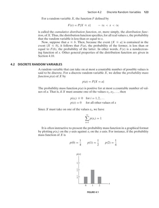
140. Section 4.3 Expected Value 125
the value of F is constant in the intervals [xi−1, xi) and then takes a step (or jump) of
size p(xi) at xi. For instance, if X has a probability mass function given by
p(1) =
1
4
p(2) =
1
2
p(3) =
1
8
p(4) =
1
8
then its cumulative distribution function is
F(a) =
⎧
⎪
⎪
⎪
⎪
⎪
⎪
⎪
⎪
⎨
⎪
⎪
⎪
⎪
⎪
⎪
⎪
⎪
⎩
0 a 1
1
4 1 … a 2
3
4 2 … a 3
7
8 3 … a 4
1 4 … a
This function is depicted graphically in Figure 4.3.
1
–
4
1
1 2 3
a
F(a)
4
3
–
4
7
–
8
FIGURE 4.3
Note that the size of the step at any of the values 1, 2, 3, and 4 is equal to the
probability that X assumes that particular value.
4.3 EXPECTED VALUE
One of the most important concepts in probability theory is that of the expectation
of a random variable. If X is a discrete random variable having a probability mass
function p(x), then the expectation, or the expected value, of X, denoted by E[X], is
defined by
E[X] =
x:p(x)0
xp(x)
In words, the expected value of X is a weighted average of the possible values that
X can take on, each value being weighted by the probability that X assumes it. For
instance, on the one hand, if the probability mass function of X is given by
p(0) =
1
2
= p(1)
then
E[X] = 0
1
2
+ 1
1
2
=
1
2

141. 126 Chapter 4 Random Variables
is just the ordinary average of the two possible values, 0 and 1, that X can assume.
On the other hand, if
p(0) =
1
3
p(1) =
2
3
then
E[X] = 0
1
3
+ 1
2
3
=
2
3
is a weighted average of the two possible values 0 and 1, where the value 1 is given
twice as much weight as the value 0, since p(1) = 2p(0).
Another motivation of the definition of expectation is provided by the frequency
interpretation of probabilities. This interpretation (partially justified by the strong
law of large numbers, to be presented in Chapter 8) assumes that if an infinite sequence
of independent replications of an experiment is performed, then, for any event E,
the proportion of time that E occurs will be P(E). Now, consider a random vari-
able X that must take on one of the values x1, x2, ... xn with respective probabilities
p(x1), p(x2), ... , p(xn), and think of X as representing our winnings in a single game of
chance. That is, with probability p(xi) we shall win xi units i = 1, 2, ... , n. By the fre-
quency interpretation, if we play this game continually, then the proportion of time
that we win xi will be p(xi). Since this is true for all i, i = 1, 2, ... , n, it follows that our
average winnings per game will be
n
i=1
xip(xi) = E[X]
EXAMPLE 3a
Find E[X], where X is the outcome when we roll a fair die.
Solution. Since p(1) = p(2) = p(3) = p(4) = p(5) = p(6) = 1
6 , we obtain
E[X] = 1
1
6
+ 2
1
6
+ 3
1
6
+ 4
1
6
+ 5
1
6
+ 6
1
6
=
7
2 .
EXAMPLE 3b
We say that I is an indicator variable for the event A if
I =
%
1 if A occurs
0 if Ac occurs
Find E[I].
Solution. Since p(1) = P(A), p(0) = 1 − P(A), we have
E[I] = P(A)
That is, the expected value of the indicator variable for the event A is equal to the
probability that A occurs. .

142. Section 4.3 Expected Value 127
EXAMPLE 3c
A contestant on a quiz show is presented with two questions, questions 1 and 2, which
he is to attempt to answer in some order he chooses. If he decides to try question i
first, then he will be allowed to go on to question j, j Z i, only if his answer to question
i is correct. If his initial answer is incorrect, he is not allowed to answer the other ques-
tion. The contestant is to receive Vi dollars if he answers question i correctly, i = 1, 2.
For instance, he will receive V1 + V2 dollars if he answers both questions correctly.
If the probability that he knows the answer to question i is Pi, i = 1, 2, which question
should he attempt to answer first so as to maximize his expected winnings? Assume
that the events Ei, i = 1, 2, that he knows the answer to question i are independent
events.
Solution. On the one hand, if he attempts to answer question 1 first, then he will win
0 with probability 1 − P1
V1 with probability P1(1 − P2)
V1 + V2 with probability P1P2
Hence, his expected winnings in this case will be
V1P1(1 − P2) + (V1 + V2)P1P2
On the other hand, if he attempts to answer question 2 first, his expected winnings
will be
V2P2(1 − P1) + (V1 + V2)P1P2
Therefore, it is better to try question 1 first if
V1P1(1 − P2) Ú V2P2(1 − P1)
or, equivalently, if
V1P1
1 − P1
Ú
V2P2
1 − P2
For example, if he is 60 percent certain of answering question 1, worth $200, correctly
and he is 80 percent certain of answering question 2, worth $100, correctly, then he
should attempt to answer question 2 first because
400 =
(100)(.8)
.2
(200)(.6)
.4
= 300 .
EXAMPLE 3d
A school class of 120 students is driven in 3 buses to a symphonic performance. There
are 36 students in one of the buses, 40 in another, and 44 in the third bus. When the
buses arrive, one of the 120 students is randomly chosen. Let X denote the number
of students on the bus of that randomly chosen student, and find E[X].
Solution. Since the randomly chosen student is equally likely to be any of the 120
students, it follows that
P{X = 36} =
36
120
P{X = 40} =
40
120
P{X = 44} =
44
120
Hence,
E[X] = 36
3
10
+ 40
1
3
+ 44
11
30
=
1208
30
= 40.2667

143. 128 Chapter 4 Random Variables
However, the average number of students on a bus is 120/3 = 40, showing that the
expected number of students on the bus of a randomly chosen student is larger than
the average number of students on a bus. This is a general phenomenon, and it occurs
because the more students there are on a bus, the more likely it is that a randomly
chosen student would have been on that bus. As a result, buses with many students
are given more weight than those with fewer students. (See Self-Test Problem 4.) .
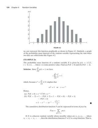
Remark. The probability concept of expectation is analogous to the physical con-
cept of the center of gravity of a distribution of mass. Consider a discrete random
variable X having probability mass function p(xi), i Ú 1. If we now imagine a weight-
less rod in which weights with mass p(xi), i Ú 1, are located at the points xi, i Ú 1
(see Figure 4.4), then the point at which the rod would be in balance is known as the
center of gravity. For those readers acquainted with elementary statics, it is now a
simple matter to show that this point is at E[X].† .
–1 0 2
^ 1
p(–1) = .10, p(0) = .25, p(2) = .35
p(1) = .30,
^ = center of gravity = .9
FIGURE 4.4
4.4 EXPECTATION OF A FUNCTION OF A RANDOM VARIABLE
Suppose that we are given a discrete random variable along with its probability mass
function and that we want to compute the expected value of some function of X,
say, g(X). How can we accomplish this? One way is as follows: Since g(X) is itself a
discrete random variable, it has a probability mass function, which can be determined
from the probability mass function of X. Once we have determined the probability
mass function of g(X), we can compute E[g(X)] by using the definition of expected
value.
EXAMPLE 4a
Let X denote a random variable that takes on any of the values −1, 0, and 1 with
respective probabilities
P{X = −1} = .2 P{X = 0} = .5 P{X = 1} = .3
Compute E[X2].
Solution. Let Y = X2. Then the probability mass function of Y is given by
P{Y = 1} = P{X = −1} + P{X = 1} = .5
P{Y = 0} = P{X = 0} = .5
Hence,
E[X2
] = E[Y] = 1(.5) + 0(.5) = .5
†To prove this, we must show that the sum of the torques tending to turn the point around E[X]
is equal to 0. That is, we must show that 0 =
i
(xi − E[X])p(xi), which is immediate.

144. Section 4.4 Expectation of a Function of a Random Variable 129
Note that
.5 = E[X2
] Z (E[X])2
= .01 .
Although the preceding procedure will always enable us to compute the expected
value of any function of X from a knowledge of the probability mass function of X,
there is another way of thinking about E[g(X)]: Since g(X) will equal g(x) whenever
X is equal to x, it seems reasonable that E[g(X)] should just be a weighted average of
the values g(x), with g(x) being weighted by the probability that X is equal to x. That
is, the following result is quite intuitive:
Proposition 4.1.
If X is a discrete random variable that takes on one of the values xi, i Ú 1, with
respective probabilities p(xi), then, for any real-valued function g,
E[g(X)] =
i
g(xi)p(xi)
Before proving this proposition, let us check that it is in accord with the results of
Example 4a. Applying it to that example yields
E{X2
} = (−1)2
(.2) + 02
(.5) + 12
(.3)
= 1(.2 + .3) + 0(.5)
= .5
which is in agreement with the result given in Example 4a.
Proof of Proposition 4.1: The proof of Proposition 4.1 proceeds, as in the preceding
verification, by grouping together all the terms in
i
g(xi)p(xi) having the same value
of g(xi). Specifically, suppose that yj, j Ú 1, represent the different values of g(xi), i Ú 1.
Then, grouping all the g(xi) having the same value gives
i
g(xi)p(xi) =
j
i:g(xi)=yj
g(xi)p(xi)
=
j
i:g(xi)=yj
yjp(xi)
=
j
yj
i:g(xi)=yj
p(xi)
=
j
yjP{g(X) = yj}
= E[g(X)]
EXAMPLE 4b
A product that is sold seasonally yields a net profit of b dollars for each unit sold and
a net loss of dollars for each unit left unsold when the season ends. The number of
units of the product that are ordered at a specific department store during any season
is a random variable having probability mass function p(i), i Ú 0. If the store must
stock this product in advance, determine the number of units the store should stock
so as to maximize its expected profit.

145. 130 Chapter 4 Random Variables
Solution. Let X denote the number of units ordered. If s units are stocked, then the
profit—call it P(s)—can be expressed as
P(s) = bX − (s − X) if X … s
= sb if X s
Hence, the expected profit equals
E[P(s)] =
s
i=0
[bi − (s − i)]p(i) +
q
i=s+1
sbp(i)
= (b + )
s
i=0
ip(i) − s
s
i=0
p(i) + sb
⎡
⎣1 −
s
i=0
p(i)
⎤
⎦
= (b + )
s
i=0
ip(i) − (b + )s
s
i=0
p(i) + sb
= sb + (b + )
s
i=0
(i − s)p(i)
To determine the optimum value of s, let us investigate what happens to the profit
when we increase s by 1 unit. By substitution, we see that the expected profit in this
case is given by
E[P(s + 1)] = b(s + 1) + (b + )
s+1
i=0
(i − s − 1)p(i)
= b(s + 1) + (b + )
s
i=0
(i − s − 1)p(i)
Therefore,
E[P(s + 1)] − E[P(s)] = b − (b + )
s
i=0
p(i)
Thus, stocking s + 1 units will be better than stocking s units whenever
s
i=0
p(i)
b
b +
(4.1)
Because the left-hand side of Equation (4.1) is increasing in s while the right-hand
side is constant, the inequality will be satisfied for all values of s … s∗, where s∗ is the
largest value of s satisfying Equation (4.1). Since
E[P(0)] · · · E[P(s∗
)] E[P(s∗
+ 1)] E[P(s∗
+ 2)] · · ·
it follows that stocking s∗ + 1 items will lead to a maximum expected profit. .
EXAMPLE 4c Utility
Suppose that you must choose one of two possible actions, each of which can result
in any of n consequences, denoted as C1, ... , Cn. Suppose that if the first action is

146. Section 4.4 Expectation of a Function of a Random Variable 131
chosen, then consequence Ci will result with probability pi, i = 1, ... , n, whereas
if the second action is chosen, then consequence Ci will result with probability qi,
i = 1, ... , n, where
n
i=1
pi =
n
i=1
qi = 1. The following approach can be used to deter-
mine which action to choose: Start by assigning numerical values to the different
consequences in the following manner: First, identify the least and the most desir-
able consequences—call them c and C, respectively; give consequence c the value 0
and give C the value 1. Now consider any of the other n − 2 consequences, say, Ci. To
value this consequence, imagine that you are given the choice between either receiv-
ing Ci or taking part in a random experiment that either earns you consequence C
with probability u or consequence c with probability 1 − u. Clearly, your choice will
depend on the value of u. On the one hand, if u = 1, then the experiment is certain
to result in consequence C, and since C is the most desirable consequence, you will
prefer participating in the experiment to receiving Ci. On the other hand, if u = 0,
then the experiment will result in the least desirable consequence—namely, c—so in
this case you will prefer the consequence Ci to participating in the experiment. Now,
as u decreases from 1 to 0, it seems reasonable that your choice will at some point
switch from participating in the experiment to the certain return of Ci, and at that
critical switch point you will be indifferent between the two alternatives. Take that
indifference probability u as the value of the consequence Ci. In other words, the
value of Ci is that probability u such that you are indifferent between either receiv-
ing the consequence Ci or taking part in an experiment that returns consequence C
with probability u or consequence c with probability 1 − u. We call this indifference
probability the utility of the consequence Ci, and we designate it as u(Ci).
To determine which action is superior, we need to evaluate each one. Consider the
first action, which results in consequence Ci with probability pi, i = 1, ... , n. We can
think of the result of this action as being determined by a two-stage experiment. In the
first stage, one of the values 1, ... , n is chosen according to the probabilities p1, ... , pn;
if value i is chosen, you receive consequence Ci. However, since Ci is equivalent to
obtaining consequence C with probability u(Ci) or consequence c with probability
1 − u(Ci), it follows that the result of the two-stage experiment is equivalent to an
experiment in which either consequence C or consequence c is obtained, with C being
obtained with probability
n
i=1
piu(Ci)
Similarly, the result of choosing the second action is equivalent to taking part in an
experiment in which either consequence C or consequence c is obtained, with C being
obtained with probability
n
i=1
qiu(Ci)
Since C is preferable to c, it follows that the first action is preferable to the second
action if
n
i=1
piu(Ci)
n
i=1
qiu(Ci)
In other words, the worth of an action can be measured by the expected value of the
utility of its consequence, and the action with the largest expected utility is the most
preferable. .

147. 132 Chapter 4 Random Variables
A simple logical consequence of Proposition 4.1 is Corollary 4.1.
Corollary 4.1. If a and b are constants, then
E[aX + b] = aE[X] + b
Proof.
E[aX + b] =
x:p(x)0
(ax + b)p(x)
= a
x:p(x)0
xp(x) + b
x:p(x)0
p(x)
= aE[X] + b
The expected value of a random variable X, E[X], is also referred to as the mean
or the first moment of X. The quantity E[Xn], n Ú 1, is called the nth moment of X.
By Proposition 4.1, we note that
E[Xn
] =
x:p(x)0
xn
p(x)
4.5 VARIANCE
Given a random variable X along with its distribution function F, it would be
extremely useful if we were able to summarize the essential properties of F by cer-
tain suitably defined measures. One such measure would be E[X], the expected value
of X. However, although E[X] yields the weighted average of the possible values of
X, it does not tell us anything about the variation, or spread, of these values. For
instance, although random variables W, Y, and Z having probability mass functions
determined by
W = 0 with probability 1
Y =
⎧
⎨
⎩
−1 with probability 1
2
+1 with probability 1
2
Z =
⎧
⎨
⎩
−100 with probability 1
2
+100 with probability 1
2
all have the same expectation—namely, 0—there is a much greater spread in the pos-
sible values of Y than in those of W (which is a constant) and in the possible values
of Z than in those of Y.
Because we expect X to take on values around its mean E[X], it would appear that
a reasonable way of measuring the possible variation of X would be to look at how
far apart X would be from its mean, on the average. One possible way to measure this
variation would be to consider the quantity E[|X − μ|], where μ = E[X]. However,
it turns out to be mathematically inconvenient to deal with this quantity, so a more
tractable quantity is usually considered—namely, the expectation of the square of the
difference between X and its mean. We thus have the following definition.

148. Section 4.5 Variance 133
Definition
If X is a random variable with mean μ, then the variance of X, denoted by Var(X),
is defined by
Var(X) = E[(X − μ)2
]
An alternative formula for Var(X) is derived as follows:
Var(X) = E[(X − μ)2
]
=
x
(x − μ)2
p(x)
=
x
(x2
− 2μx + μ2
)p(x)
=
x
x2
p(x) − 2μ
x
xp(x) + μ2
x
p(x)
= E[X2
] − 2μ2
+ μ2
= E[X2
] − μ2
That is,
Var(X) = E[X2] − (E[X])2
In words, the variance of X is equal to the expected value of X2 minus the square
of its expected value. In practice, this formula frequently offers the easiest way to
compute Var(X).
EXAMPLE 5a
Calculate Var(X) if X represents the outcome when a fair die is rolled.
Solution. It was shown in Example 3a that E[X] = 7
2. Also,
E[X2
] = 12
1
6
+ 22
1
6
+ 32
1
6
+ 42
1
6
+ 52
1
6
+ 62
1
6
=
1
6
(91)
Hence,
Var(X) =
91
6
−
7
2
2
=
35
12 .
A useful identity is that, for any constants a and b,
Var(aX + b) = a2
Var(X)

149. 134 Chapter 4 Random Variables
To prove this equality, let μ = E[X] and note from Corollary 4.1 that E[aX + b] =
aμ + b. Therefore,
Var(aX + b) = E[(aX + b − aμ − b)2
]
= E[a2
(X − μ)2
]
= a2
E[(X − μ)2
]
= a2
Var(X)
Remarks. (a) Analogous to the means being the center of gravity of a distribu-
tion of mass, the variance represents, in the terminology of mechanics, the moment
of inertia.
(b) The square root of the Var(X) is called the standard deviation of X, and we
denote it by SD(X). That is,
SD(X) =
.
Var(X)
Discrete random variables are often classified according to their probability mass
functions. In the next few sections, we consider some of the more common types.
4.6 THE BERNOULLI AND BINOMIAL RANDOM VARIABLES
Suppose that a trial, or an experiment, whose outcome can be classified as either a
success or a failure is performed. If we let X = 1 when the outcome is a success and
X = 0 when it is a failure, then the probability mass function of X is given by
p(0) = P{X = 0} = 1 − p
p(1) = P{X = 1} = p
(6.1)
where p, 0 … p … 1, is the probability that the trial is a success.
A random variable X is said to be a Bernoulli random variable (after the Swiss
mathematician James Bernoulli) if its probability mass function is given by Equa-
tions (6.1) for some p ∈ (0, 1).
Suppose now that n independent trials, each of which results in a success with prob-
ability p and in a failure with probability 1 − p, are to be performed. If X represents
the number of successes that occur in the n trials, then X is said to be a binomial
random variable with parameters (n, p). Thus, a Bernoulli random variable is just a
binomial random variable with parameters (1, p).
The probability mass function of a binomial random variable having parameters
(n, p) is given by
p(i) =
n
i
pi
(1 − p)n−i
i = 0, 1, ... , n (6.2)
The validity of Equation (6.2) may be verified by first noting that the probability of
any particular sequence of n outcomes containing i successes and n − i failures is,
by the assumed independence of trials, pi(1 − p)n−i. Equation (6.2) then follows,
since there are
n
i
different sequences of the n outcomes leading to i successes and
n − i failures. This perhaps can most easily be seen by noting that there are
n
i
different choices of the i trials that result in successes. For instance, if n = 4, i = 2,
then there are
4
2
= 6 ways in which the four trials can result in two successes,

150. Section 4.6 The Bernoulli and Binomial Random Variables 135
namely, any of the outcomes (s, s, f, f), (s, f, s, f), (s, f, f, s), (f, s, s, f), (f, s, f, s), and
(f, f, s, s), where the outcome (s, s, f, f) means, for instance, that the first two trials
are successes and the last two failures. Since each of these outcomes has probability
p2(1 − p)2 of occurring, the desired probability of two successes in the four trials
is
4
2
p2(1 − p)2.
Note that, by the binomial theorem, the probabilities sum to 1; that is,
q
i=0
p(i) =
n
i=0
ni
pi
(1 − p)n−i
= [p + (1 − p)]n
= 1
EXAMPLE 6a
Five fair coins are flipped. If the outcomes are assumed independent, find the proba-
bility mass function of the number of heads obtained.
Solution. If we let X equal the number of heads (successes) that appear, then X
is a binomial random variable with parameters
n = 5, p = 1
2
. Hence, by Equa-
tion (6.2),
P{X = 0} =
5
0
1
2
0
1
2
5
=
1
32
P{X = 1} =
5
1
1
2
1
1
2
4
=
5
32
P{X = 2} =
5
2
1
2
2
1
2
3
=
10
32
P{X = 3} =
5
3
1
2
3
1
2
2
=
10
32
P{X = 4} =
5
4
1
2
4
1
2
1
=
5
32
P{X = 5} =
5
5
1
2
5
1
2
0
=
1
32 .
EXAMPLE 6b
It is known that screws produced by a certain company will be defective with proba-
bility .01, independently of each other. The company sells the screws in packages of
10 and offers a money-back guarantee that at most 1 of the 10 screws is defective.
What proportion of packages sold must the company replace?
Solution. If X is the number of defective screws in a package, then X is a binomial
random variable with parameters (10, .01). Hence, the probability that a package will
have to be replaced is
1 − P{X = 0} − P{X = 1} = 1 −
10
0
(.01)0
(.99)10
−
10
1
(.01)1
(.99)9
L .004
Thus, only .4 percent of the packages will have to be replaced. .

151. 136 Chapter 4 Random Variables
EXAMPLE 6c
The following gambling game, known as the wheel of fortune (or chuck-a-luck), is
quite popular at many carnivals and gambling casinos: A player bets on one of the
numbers 1 through 6. Three dice are then rolled, and if the number bet by the player
appears i times, i = 1, 2, 3, then the player wins i units; if the number bet by the player
does not appear on any of the dice, then the player loses 1 unit. Is this game fair to
the player? (Actually, the game is played by spinning a wheel that comes to rest on
a slot labeled by three of the numbers 1 through 6, but this variant is mathematically
equivalent to the dice version.)
Solution. If we assume that the dice are fair and act independently of each other,
then the number of times that the number bet appears is a binomial random variable
with parameters
3, 1
6
. Hence, letting X denote the player’s winnings in the game,
we have
P{X = −1} =
3
0
1
6
0
5
6
3
=
125
216
P{X = 1} =
3
1
1
6
1
5
6
2
=
75
216
P{X = 2} =
3
2
1
6
2
5
6
1
=
15
216
P{X = 3} =
3
3
1
6
3
5
6
0
=
1
216
In order to determine whether or not this is a fair game for the player, let us calcu-
late E[X]. From the preceding probabilities, we obtain
E[X] =
−125 + 75 + 30 + 3
216
=
−17
216
Hence, in the long run, the player will lose 17 units per every 216 games he plays. .
In the next example, we consider the simplest form of the theory of inheritance as
developed by Gregor Mendel (1822–1884).
EXAMPLE 6d
Suppose that a particular trait (such as eye color or left-handedness) of a person is
classified on the basis of one pair of genes, and suppose also that d represents a dom-
inant gene and r a recessive gene. Thus, a person with dd genes is purely dominant,
one with rr is purely recessive, and one with rd is hybrid. The purely dominant and the
hybrid individuals are alike in appearance. Children receive 1 gene from each parent.
If, with respect to a particular trait, 2 hybrid parents have a total of 4 children, what is
the probability that 3 of the 4 children have the outward appearance of the dominant
gene?
Solution. If we assume that each child is equally likely to inherit either of 2 genes
from each parent, the probabilities that the child of 2 hybrid parents will have dd,
rr, and rd pairs of genes are, respectively, 1
4 , 1
4, and 1
2. Hence, since an offspring will

152. Section 4.6 The Bernoulli and Binomial Random Variables 137
have the outward appearance of the dominant gene if its gene pair is either dd or rd,
it follows that the number of such children is binomially distributed with parameters
4, 3
4
. Thus, the desired probability is
4
3
3
4
3
1
4
1
=
27
64 .
EXAMPLE 6e
Consider a jury trial in which it takes 8 of the 12 jurors to convict the defendant; that
is, in order for the defendant to be convicted, at least 8 of the jurors must vote him
guilty. If we assume that jurors act independently and that, whether or not the defen-
dant is guilty, each makes the right decision with probability θ, what is the probability
that the jury renders a correct decision?
Solution. The problem, as stated, is incapable of solution, for there is not yet enough
information. For instance, if the defendant is innocent, the probability of the jury’s
rendering a correct decision is
12
i=5
12
i
θi
(1 − θ)12−i
whereas, if he is guilty, the probability of a correct decision is
12
i=8
12
i
θi
(1 − θ)12−i
Therefore, if α represents the probability that the defendant is guilty, then, by condi-
tioning on whether or not he is guilty, we obtain the probability that the jury renders
a correct decision:
α
12
i=8
12
i
θi
(1 − θ)12−i
+ (1 − α)
12
i=5
12
i
θi
(1 − θ)12−i
.
EXAMPLE 6f
A communication system consists of n components, each of which will, indepen-
dently, function with probability p. The total system will be able to operate effectively
if at least one-half of its components function.
(a) For what values of p is a 5-component system more likely to operate effectively
than a 3-component system?
(b) In general, when is a (2k + 1)-component system better than a (2k − 1)-
component system?
Solution. (a) Because the number of functioning components is a binomial random
variable with parameters (n, p), it follows that the probability that a 5-component
system will be effective is
5
3
p3
(1 − p)2
+
5
4
p4
(1 − p) + p5

153. 138 Chapter 4 Random Variables
whereas the corresponding probability for a 3-component system is
3
2
p2
(1 − p) + p3
Hence, the 5-component system is better if
10p3
(1 − p)2
+ 5p4
(1 − p) + p5
3p2
(1 − p) + p3
which reduces to
3(p − 1)2
(2p − 1) 0
or
p
1
2
(b) In general, a system with 2k + 1 components will be better than one with
2k − 1 components if (and only if) p 1
2. To prove this, consider a system of 2k + 1
components and let X denote the number of the first 2k − 1 that function. Then
P2k+1(effective) = P{X Ú k + 1} + P{X = k}(1 − (1 − p)2
)
+ P{X = k − 1}p2
which follows because the (2k + 1)-component system will be effective if either
(i) X Ú k + 1;
(ii) X = k and at least one of the remaining 2 components function; or
(iii) X = k − 1 and both of the next 2 components function.
Since
P2k−1(effective) = P{X Ú k}
= P{X = k} + P{X Ú k + 1}
we obtain
P2k+1(effective) − P2k−1(effective)
= P{X = k − 1}p2
− (1 − p)2
P{X = k}
=
2k − 1
k − 1
pk−1
(1 − p)k
p2
− (1 − p)2
2k − 1
k
pk
(1 − p)k−1
=
2k − 1
k
pk
(1 − p)k
[ p − (1 − p)] since
2k − 1
k − 1
=
2k − 1
k
0 3 p
1
2 .

154. Section 4.6 The Bernoulli and Binomial Random Variables 139
4.6.1 Properties of Binomial Random Variables
We will now examine the properties of a binomial random variable with parameters
n and p. To begin, let us compute its expected value and variance. Now,
E[Xk
] =
n
i=0
ik
n
i
pi
(1 − p)n−i
=
n
i=1
ik
n
i
pi
(1 − p)n−i
Using the identity
i
n
i
= n
n − 1
i − 1
gives
E[Xk
] = np
n
i=1
ik−1
n − 1
i − 1
pi−1
(1 − p)n−i
= np
n−1
j=0
(j + 1)k−1
n − 1
j
pj
(1 − p)n−1−j
by letting
j = i − 1
= npE[(Y + 1)k−1
]
where Y is a binomial random variable with parameters n − 1, p. Setting k = 1 in the
preceding equation yields
E[X] = np
That is, the expected number of successes that occur in n independent trials when
each is a success with probability p is equal to np. Setting k = 2 in the preceding equa-
tion, and using the preceding formula for the expected value of a binomial random
variable yields
E[X2
] = npE[Y + 1]
= np[(n − 1)p + 1]
Since E[X] = np, we obtain
Var(X) = E[X2
] − (E[X])2
= np[(n − 1)p + 1] − (np)2
= np(1 − p)
Summing up, we have shown the following:
If X is a binomial random variable with parameters n and p, then
E[X] = np
Var(X) = np(1 − p)

155. 140 Chapter 4 Random Variables
The following proposition details how the binomial probability mass function first
increases and then decreases.
Proposition 6.1. If X is a binomial random variable with parameters (n, p), where
0 p 1, then as k goes from 0 to n, P{X = k} first increases monotonically and
then decreases monotonically, reaching its largest value when k is the largest integer
less than or equal to (n + 1)p.
Proof. We prove the proposition by considering P{X = k}/P{X = k − 1} and
determining for what values of k it is greater or less than 1. Now,
P{X = k}
P{X = k − 1}
=
n!
(n − k)!k!
pk
(1 − p)n−k
n!
(n − k + 1)!(k − 1)!
pk−1
(1 − p)n−k+1
=
(n − k + 1)p
k(1 − p)
Hence, P{X = k} Ú P{X = k − 1} if and only if
(n − k + 1)p Ú k(1 − p)
or, equivalently, if and only if
k … (n + 1)p
and the proposition is proved. .
As an illustration of Proposition 6.1 consider Figure 4.5, the graph of the probabil-
ity mass function of a binomial random variable with parameters (10, 1
2 ).
EXAMPLE 6g
In a U.S. presidential election, the candidate who gains the maximum number of
votes in a state is awarded the total number of electoral college votes allocated to
0
k
1024 ⫻ p(k)
1 2 3 4 5 6 7 8 9 10
10
45
120
210
252
1
FIGURE 4.5 Graph of p(k) =
10
k
1
2
10

156. Section 4.6 The Bernoulli and Binomial Random Variables 141
that state. The number of electoral college votes of a given state is roughly propor-
tional to the population of that state—that is, a state with population n has roughly
nc electoral votes. (Actually, it is closer to nc + 2, as a state is given an electoral
vote for each member it has in the House of Representatives, with the number of
such representatives being roughly proportional to the population of the state, and
one electoral college vote for each of its two senators.) Let us determine the average
power of a citizen in a state of size n in a close presidential election, where, by average
power in a close election, we mean that a voter in a state of size n = 2k + 1 will be
decisive if the other n − 1 voters split their votes evenly between the two candidates.
(We are assuming here that n is odd, but the case where n is even is quite similar.)
Because the election is close, we shall suppose that each of the other n − 1 = 2k
voters acts independently and is equally likely to vote for either candidate. Hence,
the probability that a voter in a state of size n = 2k + 1 will make a difference to
the outcome is the same as the probability that 2k tosses of a fair coin land heads and
tails an equal number of times. That is,
P{voter in state of size 2k + 1 makes a difference}
=
2k
k
1
2
k
1
2
k
=
(2k)!
k!k!22k
To approximate the preceding equality, we make use of Stirling’s approximation,
which says that, for k large,
k! ∼ kk+1/2
e−k
√
2π
where we say that ak ∼ bk when the ratio ak/bk approaches 1 as k approaches q.
Hence, it follows that
P{voter in state of size 2k + 1 makes a difference}
∼
(2k)2k+1/2e−2k
√
2π
k2k+1e−2k(2π)22k
=
1
√
kπ
Because such a voter (if he or she makes a difference) will affect nc electoral votes,
the expected number of electoral votes a voter in a state of size n will affect—or the
voter’s average power—is given by
average power = ncP{makes a difference}
∼
nc
.
nπ/2
= c
.
2n/π
Thus, the average power of a voter in a state of size n is proportional to the square
root of n, showing that, in presidential elections, voters in large states have more
power than do those in smaller states. .

157. 142 Chapter 4 Random Variables
4.6.2 Computing the Binomial Distribution Function
Suppose that X is binomial with parameters (n, p). The key to computing its distribu-
tion function
P{X … i} =
i
k=0
n
k
pk
(1 − p)n−k
i = 0, 1, ... , n
is to utilize the following relationship between P{X = k + 1} and P{X = k}, which
was established in the proof of Proposition 6.1:
P{X = k + 1} =
p
1 − p
n − k
k + 1
P{X = k} (6.3)
EXAMPLE 6h
Let X be a binomial random variable with parameters n = 6, p = .4. Then, starting
with P{X = 0} = (.6)6 and recursively employing Equation (6.3), we obtain
P{X = 0} = (.6)6
L .0467
P{X = 1} =
4
6
6
1
P{X = 0} L .1866
P{X = 2} =
4
6
5
2
P{X = 1} L .3110
P{X = 3} =
4
6
4
3
P{X = 2} L .2765
P{X = 4} =
4
6
3
4
P{X = 3} L .1382
P{X = 5} =
4
6
2
5
P{X = 4} L .0369
P{X = 6} =
4
6
1
6
P{X = 5} L .0041 .
A computer program that utilizes the recursion (6.3) to compute the binomial
distribution function is easily written. To compute P{X … i}, the program should
first compute P{X = i} and then use the recursion to successively compute P{X =
i − 1}, P{X = i − 2}, and so on.
Historical Note
Independent trials having a common probability of success p were first studied
by the Swiss mathematician Jacques Bernoulli (1654–1705). In his book Ars Con-
jectandi (The Art of Conjecturing), published by his nephew Nicholas eight years
after his death in 1713, Bernoulli showed that if the number of such trials were
large, then the proportion of them that were successes would be close to p with a
probability near 1.
Jacques Bernoulli was from the first generation of the most famous mathemat-
ical family of all time. Altogether, there were between 8 and 12 Bernoullis, spread
over three generations, who made fundamental contributions to probability, statis-
tics, and mathematics. One difficulty in knowing their exact number is the fact that
several had the same name. (For example, two of the sons of Jacques’s brother Jean

158. Section 4.7 The Poisson Random Variable 143
were named Jacques and Jean.) Another difficulty is that several of the Bernoullis
were known by different names in different places. Our Jacques (sometimes writ-
ten Jaques) was, for instance, also known as Jakob (sometimes written Jacob) and
as James Bernoulli. But whatever their number, their influence and output were
prodigious. Like the Bachs of music, the Bernoullis of mathematics were a family
for the ages!
EXAMPLE 6i
If X is a binomial random variable with parameters n = 100 and p = .75, find P{X =
70} and P{X … 70}.
Solution. The answer is shown here in Figure 4.6.
Enter Value For p:.75
Enter Value For n:100
Enter Value For i:70
Binomial Distribution
Start
Quit
Probability (Number of Successes = i) = .04575381
Probability (Number of Successes = i) = .14954105
FIGURE 4.6
4.7 THE POISSON RANDOM VARIABLE
A random variable X that takes on one of the values 0, 1, 2, ... is said to be a Poisson
random variable with parameter λ if, for some λ 0,
p(i) = P{X = i} = e−λ λi
i!
i = 0, 1, 2, ... (7.1)
Equation (7.1) defines a probability mass function, since
q
i=0
p(i) = e−λ
q
i=0
λi
i!
= e−λ
eλ
= 1
The Poisson probability distribution was introduced by Siméon Denis Poisson in a
book he wrote regarding the application of probability theory to lawsuits, criminal
trials, and the like. This book, published in 1837, was entitled Recherches sur la prob-
abilité des jugements en matière criminelle et en matière civile (Investigations into the
Probability of Verdicts in Criminal and Civil Matters).
The Poisson random variable has a tremendous range of applications in diverse
areas because it may be used as an approximation for a binomial random variable
with parameters (n, p) when n is large and p is small enough so that np is of moderate

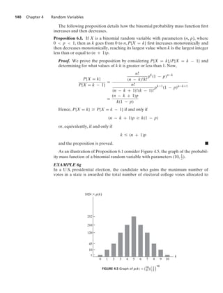
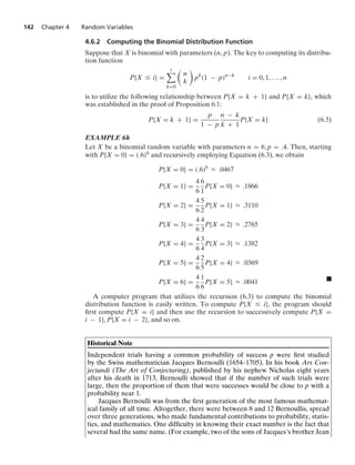
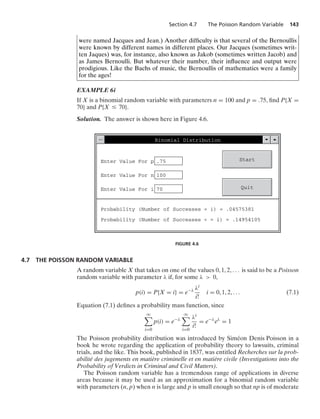
159. 144 Chapter 4 Random Variables
size. To see this, suppose that X is a binomial random variable with parameters (n, p),
and let λ = np. Then
P{X = i} =
n!
(n − i)!i!
pi
(1 − p)n−i
=
n!
(n − i)!i!
λ
n
i
1 −
λ
n
n−i
=
n(n − 1) · · · (n − i + 1)
ni
λi
i!
(1 − λ/n)n
(1 − λ/n)i
Now, for n large and λ moderate,
1 −
λ
n
n
L e−λ n(n − 1) · · · (n − i + 1)
ni
L 1
1 −
λ
n
i
L 1
Hence, for n large and λ moderate,
P{X = i} L e−λ λi
i!
In other words, if n independent trials, each of which results in a success with
probability p, are performed, then, when n is large and p is small enough to make
np moderate, the number of successes occurring is approximately a Poisson random
variable with parameter λ = np. This value λ (which will later be shown to equal the
expected number of successes) will usually be determined empirically.
Some examples of random variables that generally obey the Poisson probability
law [that is, they obey Equation (7.1)] are as follows:
1. The number of misprints on a page (or a group of pages) of a book
2. The number of people in a community who survive to age 100
3. The number of wrong telephone numbers that are dialed in a day
4. The number of packages of dog biscuits sold in a particular store each day
5. The number of customers entering a post office on a given day
6. The number of vacancies occurring during a year in the federal judicial system
7. The number of α-particles discharged in a fixed period of time from some radioac-
tive material
Each of the preceding, and numerous other random variables, are approximately
Poisson for the same reason—namely, because of the Poisson approximation to the
binomial. For instance, we can suppose that there is a small probability p that each
letter typed on a page will be misprinted. Hence, the number of misprints on a page
will be approximately Poisson with λ = np, where n is the number of letters on a
page. Similarly, we can suppose that each person in a community has some small
probability of reaching age 100. Also, each person entering a store may be thought of
as having some small probability of buying a package of dog biscuits, and so on.
EXAMPLE 7a
Suppose that the number of typographical errors on a single page of this book has a
Poisson distribution with parameter λ = 1
2 . Calculate the probability that there is at
least one error on this page.

160. Section 4.7 The Poisson Random Variable 145
Solution. Letting X denote the number of errors on this page, we have
P{X Ú 1} = 1 − P{X = 0} = 1 − e−1/2
L .393 .
EXAMPLE 7b
Suppose that the probability that an item produced by a certain machine will be
defective is .1. Find the probability that a sample of 10 items will contain at most
1 defective item.
Solution. The desired probability is
10
0
(.1)0(.9)10 +
10
1
(.1)1(.9)9 = .7361,
whereas the Poisson approximation yields the value e−1 + e−1 L .7358. .
EXAMPLE 7c
Consider an experiment that consists of counting the number of α particles given
off in a 1-second interval by 1 gram of radioactive material. If we know from past
experience that, on the average, 3.2 such α particles are given off, what is a good
approximation to the probability that no more than 2 α particles will appear?
Solution. If we think of the gram of radioactive material as consisting of a large num-
ber n of atoms, each of which has probability of 3.2/n of disintegrating and sending off
an α particle during the second considered, then we see that, to a very close approx-
imation, the number of α particles given off will be a Poisson random variable with
parameter λ = 3.2. Hence, the desired probability is
P{X … 2} = e−3.2
+ 3.2e−3.2
+
(3.2)2
2
e−3.2
L .3799 .
Before computing the expected value and variance of the Poisson random variable
with parameter λ, recall that this random variable approximates a binomial random
variable with parameters n and p when n is large, p is small, and λ = np. Since such
a binomial random variable has expected value np = λ and variance np(1 − p) =
λ(1 − p) L λ (since p is small), it would seem that both the expected value and the
variance of a Poisson random variable would equal its parameter λ. We now verify
this result:
E[X] =
q
i=0
ie−λλi
i!
= λ
q
i=1
e−λλi−1
(i − 1)!
= λe−λ
q
j=0
λj
j!
by letting
j = i − 1
= λ since
q
j=0
λj
j!
= eλ

161. 146 Chapter 4 Random Variables
Thus, the expected value of a Poisson random variable X is indeed equal to its
parameter λ. To determine its variance, we first compute E[X2]:
E[X2
] =
q
i=0
i2e−λλi
i!
= λ
q
i=1
ie−λλi−1
(i − 1)!
= λ
q
j=0
(j + 1)e−λλj
j!
by letting
j = i − 1
= λ
⎡
⎢
⎣
q
j=0
je−λλj
j!
+
q
j=0
e−λλj
j!
⎤
⎥
⎦
= λ(λ + 1)
where the final equality follows because the first sum is the expected value of a Pois-
son random variable with parameter λ and the second is the sum of the probabilities
of this random variable. Therefore, since we have shown that E[X] = λ, we obtain
Var(X) = E[X2
] − (E[X])2
= λ
Hence, the expected value and variance of a Poisson random variable are both
equal to its parameter λ.
We have shown that the Poisson distribution with parameter np is a very good
approximation to the distribution of the number of successes in n independent trials
when each trial has probability p of being a success, provided that n is large and p
small. In fact, it remains a good approximation even when the trials are not inde-
pendent, provided that their dependence is weak. For instance, recall the matching
problem (Example 5m of Chapter 2) in which n men randomly select hats from a set
consisting of one hat from each person. From the point of view of the number of men
who select their own hat, we may regard the random selection as the result of n tri-
als where we say that trial i is a success if person i selects his own hat, i = 1, ... , n.
Defining the events Ei, i = 1, ... , n, by
Ei = {trial i is a success}
it is easy to see that
P{Ei} =
1
n
and P{Ei|Ej} =
1
n − 1
, j Z i
Thus, we see that, although the events Ei, i = 1, ... , n are not independent, their
dependence, for large n, appears to be weak. Because of this it seems reasonable to
expect that the number of successes will approximately have a Poisson distribution
with parameter n * 1/n = 1, and indeed this is verified in Example 5m of Chapter 2.
For a second illustration of the strength of the Poisson approximation when the
trials are weakly dependent, let us consider again the birthday problem presented in
Example 5i of Chapter 2. In this example, we suppose that each of n people is equally
likely to have any of the 365 days of the year as his or her birthday, and the problem

162. Section 4.7 The Poisson Random Variable 147
is to determine the probability that a set of n independent people all have different
birthdays. A combinatorial argument was used to determine this probability, which
was shown to be less than 1
2 when n = 23.
We can approximate the preceding probability by using the Poisson approximation
as follows: Imagine that we have a trial for each of the
n
2
pairs of individuals i and
j, i Z j, and say that trial i, j is a success if persons i and j have the same birthday. If
we let Eij denote the event that trial i, j is a success, then, whereas the
n
2
events
Eij, 1 … i j … n, are not independent (see Theoretical Exercise 21), their depen-
dence appears to be rather weak. (Indeed, these events are even pairwise indepen-
dent, in that any 2 of the events Eij and Ekl are independent—again, see Theoretical
Exercise 21). Since P(Eij) = 1/365, it is reasonable to suppose that the number of
successes should approximately have a Poisson distribution with mean
n
2
365 =
n(n − 1)/730. Therefore,
P{no 2 people have the same birthday} = P{0 successes}
L exp
%
−n(n − 1)
730
/
To determine the smallest integer n for which this probability is less than 1
2, note that
exp
%
−n(n − 1)
730
/
…
1
2
is equivalent to
exp
%
n(n − 1)
730
/
Ú 2
Taking logarithms of both sides, we obtain
n(n − 1) Ú 730 log 2
L 505.997
which yields the solution n = 23, in agreement with the result of Example 5i of
Chapter 2.
Suppose now that we wanted the probability that, among the n people, no 3 of
them have their birthday on the same day. Whereas this now becomes a difficult com-
binatorial problem, it is a simple matter to obtain a good approximation. To begin,
imagine that we have a trial for each of the
n
3
triplets i, j, k, where 1 … i j k … n,
and call the i, j, k trial a success if persons i, j, and k all have their birthday on the same
day. As before, we can then conclude that the number of successes is approximately
a Poisson random variable with parameter
n
3
P{i, j, k have the same birthday} =
n
3
1
365
2
=
n(n − 1)(n − 2)
6 * (365)2

163. 148 Chapter 4 Random Variables
Hence,
P{no 3 have the same birthday} L exp
%
−n(n − 1)(n − 2)
799350
/
This probability will be less than 1
2 when n is such that
n(n − 1)(n − 2) Ú 799350 log 2 L 554067.1
which is equivalent to n Ú 84. Thus, the approximate probability that at least 3 people
in a group of size 84 or larger will have the same birthday exceeds 1
2 .
For the number of events to occur to approximately have a Poisson distribution, it
is not essential that all the events have the same probability of occurrence, but only
that all of these probabilities be small. The following is referred to as the Poisson
paradigm.
Poisson Paradigm. Consider n events, with pi equal to the probability that event i
occurs, i = 1, ... , n. If all the pi are “small” and the trials are either independent or at
most “weakly dependent,” then the number of these events that occur approximately
has a Poisson distribution with mean n
i=1 pi.
Our next example not only makes use of the Poisson paradigm, but also illustrates
a variety of the techniques we have studied so far.
EXAMPLE 7d Length of the longest run
A coin is flipped n times. Assuming that the flips are independent, with each one
coming up heads with probability p, what is the probability that there is a string of k
consecutive heads?
Solution. We will first use the Poisson paradigm to approximate this probability.
Now, if, for i = 1, ... , n − k + 1, we let Hi denote the event that flips i, i + 1, ... , i +
k − 1 all land on heads, then the desired probability is that at least one of the events
Hi occur. Because Hi is the event that, starting with flip i, the next k flips all land on
heads, it follows that P(Hi) = pk. Thus, when pk is small, we might think that the num-
ber of the Hi that occur should have an approximate Poisson distribution. However,
such is not the case, because, although the events all have small probabilities, some of
their dependencies are too great for the Poisson distribution to be a good approxima-
tion. For instance, because the conditional probability that flips 2, ... , k + 1 are all
heads given that flips 1, ... , k are all heads is equal to the probability that flip k + 1
is a head, it follows that
P(H2|H1) = p
which is far greater than the unconditional probability of H2.
The trick that enables us to use a Poisson approximation is to note that there
will be a string of k consecutive heads either if there is such a string that is imme-
diately followed by a tail or if the final k flips all land on heads. Consequently, for
i = 1, ... , n − k, let Ei be the event that flips i, ... , i + k − 1 are all heads and flip
i + k is a tail; also, let En−k+1 be the event that flips n − k + 1, ... , n are all heads.
Note that
P(Ei) = pk
(1 − p), i … n − k
P(En−k+1) = pk

164. Section 4.7 The Poisson Random Variable 149
Thus, when pk is small, each of the events Ei has a small probability of occurring.
Moreover, for i Z j, if the events Ei and Ej refer to nonoverlapping sequences of flips,
then P(Ei|Ej) = P(Ei); if they refer to overlapping sequences, then P(Ei|Ej) = 0.
Hence, in both cases, the conditional probabilities are close to the unconditional ones,
indicating that N, the number of the events Ei that occur, should have an approximate
Poisson distribution with mean
E[N] =
n−k+1
i=1
P(Ei) = (n − k)pk
(1 − p) + pk
Because there will not be a run of k heads if (and only if) N = 0, thus the preceding
gives
P(no head strings of length k) = P(N = 0) L exp{−(n − k)pk
(1 − p) − pk
}
If we let Ln denote the largest number of consecutive heads in the n flips, then,
because Ln will be less than k if (and only if) there are no head strings of length
k, the preceding equation can be written as
P{Ln k} L exp{− (n − k)pk
(1 − p) − pk
}
Now, let us suppose that the coin being flipped is fair; that is, suppose that p = 1/2.
Then the preceding gives
P{Ln k} L exp
%
−
n − k + 2
2k+1
/
L exp
%
−
n
2k+1
/
where the final approximation supposes that e
k−2
2k+1 L 1 (that is, that k−2
2k+1 L 0). Let
j = log2 n, and assume that j is an integer. For k = j + i,
n
2k+1
=
n
2j2i+1
=
1
2i+1
Consequently,
P{Ln j + i} L exp{−(1/2)i+1
}
which implies that
P{Ln = j + i} = P{Ln j + i + 1} − P{Ln j + i}
L exp{−(1/2)i+2
} − exp{−(1/2)i+1
}
For instance,
P{Ln j − 3} L e−4
L .0183
P{Ln = j − 3} L e−2
− e−4
L .1170
P{Ln = j − 2} L e−1
− e−2
L .2325
P{Ln = j − 1} L e−1/2
− e−1
L .2387
P{Ln = j} L e−1/4
− e−1/2
L .1723
P{Ln = j + 1} L e−1/8
− e−1/4
L .1037
P{Ln = j + 2} L e−1/16
− e−1/8
L .0569
P{Ln = j + 3} L e−1/32
− e−1/16
L .0298
P{Ln Ú j + 4} L 1 − e−1/32
L .0308

165. 150 Chapter 4 Random Variables
Thus, we observe the rather interesting fact that no matter how large n is, the length
of the longest run of heads in a sequence of n flips of a fair coin will be within 2 of
log2(n) − 1 with a probability approximately equal to .86.
We now derive an exact expression for the probability that there is a string of
k consecutive heads when a coin that lands on heads with probability p is flipped
n times. With the events Ei, i = 1, ... , n − k + 1, as defined earlier, and with Ln
denoting, as before, the length of the longest run of heads,
P(Ln Ú k) = P(there is a string of k consecutive heads) = P(∪n−k+1
i=1 Ei)
The inclusion–exclusion identity for the probability of a union can be written as
P(∪n−k+1
i=1 Ei) =
n−k+1
r=1
(−1)r+1
i1···ir
P(Ei1
· · · Eir )
Let Si denote the set of flip numbers to which the event Ei refers. (So, for instance,
S1 = {1, ... , k + 1}.) Now, consider one of the r-way intersection probabilities that
does not include the event En−k+1. That is, consider P(Ei1
· · · Eir ) where i1 · · ·
ir n − k + 1. On the one hand, if there is any overlap in the sets Si1
, ... , Sir then this
probability is 0. On the other hand, if there is no overlap, then the events Ei1
, ... , Eir
are independent. Therefore,
P(Ei1
· · · Eir ) =
0
0, if there is any overlap in Si1
, ... , Sir
prk(1 − p)r, if there is no overlap
We must now determine the number of different choices of i1 · · · ir n − k + 1
for which there is no overlap in the sets Si1
, ... , Sir . To do so, note first that each of
the Sij , j = 1, ... , r, refer to k + 1 flips, so, without any overlap, they together refer
to r(k + 1) flips. Now consider any permutation of r identical letters a (one for each
of the sets Si1
, ... , Sir−1
) and of n − r(k + 1) identical letters b (one for each of the
trials that are not part of any of Si1
, ... , Sir−1
, Sn−k+1). Interpret the number of b’s
before the first a as the number of flips before Si1
, the number of b’s between the first
and second a as the number of flips between Si1
and Si2 , and so on, with the number
of b’s after the final a representing the number of flips after Sir . Because there are
n−rk
r
permutations of r letters a and of n − r(k + 1) letters b, with every such
permutation corresponding (in a one-to-one fashion) to a different nonoverlapping
choice, it follows that
i1···irn−k+1
P(Ei1
· · · Eir ) =
n − rk
r
prk
(1 − p)r
We must now consider r-way intersection probabilities of the form
P(Ei1
· · · Eir−1
En−k+1),
where i1 · · · ir−1 n − k + 1. Now, this probability will equal 0 if there is any
overlap in Si1
, ... , Sir−1
, Sn−k; if there is no overlap, then the events of the intersection
will be independent, so
P(Ei1
· · · Eir−1
En−k+1) = [pk
(1 − p)]r−1
pk
= pkr
(1 − p)r−1
By a similar argument as before, the number of nonoverlapping sets Si1
, ... , Sir−1
, Sn−k
will equal the number of permutations of r − 1 letters a (one for each of the sets

166. Section 4.7 The Poisson Random Variable 151
Si1
, ... , Sir−1
) and of n − (r − 1)(k + 1) − k = n − rk − (r − 1) letters b (one
for each of the trials that are not part of any of Si1
, ... , Sir−1
, Sn−k+1). Since there are
n−rk
r−1
permutations of r − 1 letters a and of n − rk − (r − 1) letters b, we have
i1...ir−1n−k+1
P(Ei1
· · · Eir−1
En−k+1) =
n − rk
r − 1
pkr
(1 − p)r−1
Putting it all together yields the exact expression, namely,
P(Ln Ú k) =
n−k+1
r=1
(−1)r+1
n − rk
r
+
1
p
n − rk
r − 1
pkr
(1 − p)r
where we utilize the convention that
m
j
= 0 if m j.
From a computational point of view, a more efficient method for computing the
desired probability than the use of the preceding identity is to derive a set of recur-
sive equations. To do so, let An be the event that there is a string of k consecutive
heads in a sequence of n flips of a fair coin, and let Pn = P(An). We will derive a
set of recursive equations for Pn by conditioning on when the first tail appears. For
j = 1, ... , k, let Fj be the event that the first tail appears on flip j, and let H be the
event that the first k flips are all heads. Because the events F1, ... , Fk, H are mutually
exclusive and exhaustive (that is, exactly one of these events must occur), we have
P(An) =
k
j=1
P(An|Fj)P(Fj) + P(An|H)P(H)
Now, given that the first tail appears on flip j, where j k, it follows that those j
flips are wasted as far as obtaining a string of k heads in a row; thus, the conditional
probability of this event is the probability that such a string will occur among the
remaining n − j flips. Therefore,
P(An|Fj) = Pn−j
Because P(An|H) = 1, the preceding equation gives
Pn = P(An)
=
k
j=1
Pn−j P(Fj) + P(H)
=
k
j=1
Pn−j pj−1
(1 − p) + pk
Starting with Pj = 0, j k, and Pk = pk, we can use the latter formula to recursively
compute Pk+1, Pk+2, and so on, up to Pn. For instance, suppose we want the prob-
ability that there is a run of 2 consecutive heads when a fair coin is flipped 4 times.
Then, with k = 2, we have P1 = 0, P2 = (1/2)2. Because, when p = 1/2, the recursion
becomes
Pn =
k
j=1
Pn−j (1/2)j
+ (1/2)k

167. 152 Chapter 4 Random Variables
we obtain
P3 = P2(1/2) + P1(1/2)2
+ (1/2)2
= 3/8
and
P4 = P3(1/2) + P2(1/2)2
+ (1/2)2
= 1/2
which is clearly true because there are 8 outcomes that result in a string of 2 consec-
utive heads: hhhh, hhht, hhth, hthh, thhh, hhtt, thht, and tthh. Each of these outcomes
occurs with probability 1/16. .
Another use of the Poisson probability distribution arises in situations where
“events” occur at certain points in time. One example is to designate the occurrence
of an earthquake as an event; another possibility would be for events to correspond
to people entering a particular establishment (bank, post office, gas station, and so
on); and a third possibility is for an event to occur whenever a war starts. Let us sup-
pose that events are indeed occurring at certain (random) points of time, and let us
assume that, for some positive constant λ, the following assumptions hold true:
1. The probability that exactly 1 event occurs in a given interval of length h is equal
to λh + o(h), where o(h) stands for any function f(h) for which lim
h→0
f(h)/h = 0.
[For instance, f(h) = h2 is o(h), whereas f(h) = h is not.]
2. The probability that 2 or more events occur in an interval of length h is equal
to o(h).
3. For any integers n, j1, j2, ... , jn and any set of n nonoverlapping intervals, if we
define Ei to be the event that exactly ji of the events under consideration occur
in the ith of these intervals, then events E1, E2, ... , En are independent.
Loosely put, assumptions 1 and 2 state that, for small values of h, the probability
that exactly 1 event occurs in an interval of size h equals λh plus something that is
small compared with h, whereas the probability that 2 or more events occur is small
compared with h. Assumption 3 states that whatever occurs in one interval has no
(probability) effect on what will occur in other, nonoverlapping intervals.
We now show that, under assumptions 1, 2, and 3, the number of events occurring
in any interval of length t is a Poisson random variable with parameter λt. To be
precise, let us call the interval [0, t] and denote the number of events occurring in that
interval by N(t). To obtain an expression for P{N(t) = k}, we start by breaking the
interval [0, t] into n nonoverlapping subintervals, each of length t/n (Figure 4.7).
Now,
P{N(t) = k} = P{k of the n subintervals contain exactly 1 event
and the other n − k contain 0 events} (7.2)
+ P{N(t) = k and at least 1 subinterval contains
2 or more events}
The proceding equation holds because the event on the left side of Equation (7.2),
that is, {N(t) = k}, is clearly equal to the union of the two mutually exclusive events
0
t
–
n
2t
—
n
3t
—
n
t
–
n
(n – 1)
nt
—
n
t =
FIGURE 4.7

168. Section 4.7 The Poisson Random Variable 153
on the right side of the equation. Letting A and B denote the two mutually exclusive
events on the right side of Equation (7.2), we have
P(B) … P{at least one subinterval contains 2 or more events}
= P
⎛
⎝
n
i=1
{ith subinterval contains 2 or more events}
⎞
⎠
…
n
i=1
P{ith subinterval contains 2 or more events}
by Boole’s
inequality
=
n
i=1
o
t
n
by assumption 2
= no
t
n
= t
o(t/n)
t/n
Now, in addition for any t, t/n→0 as n→q, so o(t/n)/(t/n)→0 as n→q, by the defini-
tion of o(h). Hence,
P(B)→0 as n→q (7.3)
Moreover, since assumptions 1 and 2 imply that†
P{0 events occur in an interval of length h}
= 1 − [λh + o(h) + o(h)] = 1 − λh − o(h)
we see from the independence assumption (number 3) that
P(A) = P{k of the subintervals contain exactly 1 event and the other
n − k contain 0 events}
=
n
k
λt
n
+ o
t
n
k
1 −
λt
n
− o
t
n
n−k
However, since
n
λt
n
+ o
t
n
= λt + t
o(t/n)
t/n
→λt as n→q
it follows, by the same argument that verified the Poisson approximation to the bino-
mial, that
P(A)→e−λt (λt)k
k!
as n→q (7.4)
Thus, from Equations (7.2), (7.3), and (7.4), by letting n→q, we obtain
P{N(t) = k} = e−λt (λt)k
k!
k = 0, 1, ... (7.5)
†The sum of two functions, both of which are o(h), is also o(h). This is so because if
limh→0 f(h)/h = limh→0 g(h)/h = 0, then limh→0[f(h) + g(h)]/h = 0.

169. 154 Chapter 4 Random Variables
Hence, if assumptions 1, 2, and 3 are satisfied, then the number of events occurring
in any fixed interval of length t is a Poisson random variable with mean λt, and we say
that the events occur in accordance with a Poisson process having rate λ. The value λ,
which can be shown to equal the rate per unit time at which events occur, is a constant
that must be empirically determined.
The preceding discussion explains why a Poisson random variable is usually a good
approximation for such diverse phenomena as the following:
1. The number of earthquakes occurring during some fixed time span
2. The number of wars per year
3. The number of electrons emitted from a heated cathode during a fixed time
period
4. The number of deaths, in a given period of time, of the policyholders of a life
insurance company
EXAMPLE 7e
Suppose that earthquakes occur in the western portion of the United States in accor-
dance with assumptions 1, 2, and 3, with λ = 2 and with 1 week as the unit of time.
(That is, earthquakes occur in accordance with the three assumptions at a rate of 2
per week.)
(a) Find the probability that at least 3 earthquakes occur during the next 2 weeks.
(b) Find the probability distribution of the time, starting from now, until the next
earthquake.
Solution. (a) From Equation (7.5), we have
P{N(2) Ú 3} = 1 − P{N(2) = 0} − P{N(2) = 1} − P{N(2) = 2}
= 1 − e−4
− 4e−4
−
42
2
e−4
= 1 − 13e−4
(b) Let X denote the amount of time (in weeks) until the next earthquake. Because
X will be greater than t if and only if no events occur within the next t units of time,
we have, from Equation (7.5),
P{X t} = P{N(t) = 0} = e−λt
so the probability distribution function F of the random variable X is given by
F(t) = P{X … t} = 1 − P{X t} = 1 − e−λt
= 1 − e−2t
.
4.7.1 Computing the Poisson Distribution Function
If X is Poisson with parameter λ, then
P{X = i + 1}
P{X = i}
=
e−λλi+1/(i + 1)!
e−λλi/i!
=
λ
i + 1
(7.6)

170. Section 4.8 Other Discrete Probability Distributions 155
Starting with P{X = 0} = e−λ, we can use (7.6) to compute successively
P{X = 1} = λP{X = 0}
P{X = 2} =
λ
2
P{X = 1}
.
.
.
P{X = i + 1} =
λ
i + 1
P{X = i}
The website includes a program that uses Equation (7.6) to compute Poisson prob-
abilities.
EXAMPLE 7f
(a) Determine P{X … 90} when X is Poisson with mean 100.
(b) Determine P{Y … 1075} when Y is Poisson with mean 1000.
Solution. From the website, we obtain the solutions:
(a) P{X … 90} L .1714;
(b) P{Y … 1075} L .9894. .
4.8 OTHER DISCRETE PROBABILITY DISTRIBUTIONS
4.8.1 The Geometric Random Variable
Suppose that independent trials, each having a probability p, 0 p 1, of being a
success, are performed until a success occurs. If we let X equal the number of trials
required, then
P{X = n} = (1 − p)n−1
p n = 1, 2, ... (8.1)
Equation (8.1) follows because, in order for X to equal n, it is necessary and sufficient
that the first n − 1 trials are failures and the nth trial is a success. Equation (8.1) then
follows, since the outcomes of the successive trials are assumed to be independent.
Since
q
n=1
P{X = n} = p
q
n=1
(1 − p)n−1
=
p
1 − (1 − p)
= 1
it follows that, with probability 1, a success will eventually occur. Any random vari-
able X whose probability mass function is given by Equation (8.1) is said to be a
geometric random variable with parameter p.
EXAMPLE 8a
An urn contains N white and M black balls. Balls are randomly selected, one at a
time, until a black one is obtained. If we assume that each ball selected is replaced
before the next one is drawn, what is the probability that
(a) exactly n draws are needed?
(b) at least k draws are needed?
Solution. If we let X denote the number of draws needed to select a black ball, then
X satisfies Equation (8.1) with p = M/(M + N). Hence,

171. 156 Chapter 4 Random Variables
(a)
P{X = n} =
N
M + N
n−1
M
M + N
=
MNn−1
(M + N)n
(b)
P{X Ú k} =
M
M + N
q
n=k
N
M + N
n−1
=
M
M + N
N
M + N
k−1
1
1 −
N
M + N
=
N
M + N
k−1
Of course, part (b) could have been obtained directly, since the probability that at
least k trials are necessary to obtain a success is equal to the probability that the first
k − 1 trials are all failures. That is, for a geometric random variable,
P{X Ú k} = (1 − p)k−1
.
EXAMPLE 8b
Find the expected value of a geometric random variable.
Solution. With q = 1 − p, we have
E[X] =
q
i=1
iqi−1
p
=
q
i=1
(i − 1 + 1)qi−1
p
=
q
i=1
(i − 1)qi−1
p +
q
i=1
qi−1
p
=
q
j=0
jqj
p + 1
= q
q
j=1
jqj−1
p + 1
= qE[X] + 1
Hence,
pE[X] = 1
yielding the result
E[X] =
1
p

172. Section 4.8 Other Discrete Probability Distributions 157
In other words, if independent trials having a common probability p of being success-
ful are performed until the first success occurs, then the expected number of required
trials equals 1/p. For instance, the expected number of rolls of a fair die that it takes
to obtain the value 1 is 6. .
EXAMPLE 8c
Find the variance of a geometric random variable.
Solution. To determine Var(X), let us first compute E[X2]. With q = 1 − p, we have
E[X2
] =
q
i=1
i2
qi−1
p
=
q
i=1
(i − 1 + 1)2
qi−1
p
=
q
i=1
(i − 1)2
qi−1
p +
q
i=1
2(i − 1)qi−1
p +
q
i=1
qi−1
p
=
q
j=0
j2
qj
p + 2
q
j=1
jqj
p + 1
= qE[X2
] + 2qE[X] + 1
Using E[X] = 1/p, the equation for E[X2] yields
pE[X2
] =
2q
p
+ 1
Hence,
E[X2
] =
2q + p
p2
=
q + 1
p2
giving the result
Var(X) =
q + 1
p2
−
1
p2
=
q
p2
=
1 − p
p2 .
4.8.2 The Negative Binomial Random Variable
Suppose that independent trials, each having probability p, 0 p 1, of being a
success are performed until a total of r successes is accumulated. If we let X equal the
number of trials required, then
P{X = n} =
n − 1
r − 1
pr
(1 − p)n−r
n = r, r + 1, ... (8.2)
Equation (8.2) follows because, in order for the rth success to occur at the nth trial,
there must be r − 1 successes in the first n − 1 trials and the nth trial must be a
success. The probability of the first event is
n − 1
r − 1
pr−1
(1 − p)n−r

173. 158 Chapter 4 Random Variables
and the probability of the second is p; thus, by independence, Equation (8.2) is estab-
lished. To verify that a total of r successes must eventually be accumulated, either we
can prove analytically that
q
n=r
P{X = n} =
q
n=r
n − 1
r − 1
pr
(1 − p)n−r
= 1 (8.3)
or we can give a probabilistic argument as follows: The number of trials required
to obtain r successes can be expressed as Y1 + Y2 + · · · + Yr, where Y1 equals
the number of trials required for the first success, Y2 the number of additional trials
after the first success until the second success occurs, Y3 the number of additional
trials until the third success, and so on. Because the trials are independent and all
have the same probability of success, it follows that Y1, Y2, ... , Yr are all geometric
random variables. Hence, each is finite with probability 1, so
r
i=1
Yi must also be finite,
establishing Equation (8.3).
Any random variable X whose probability mass function is given by Equation (8.2)
is said to be a negative binomial random variable with parameters (r, p). Note that a
geometric random variable is just a negative binomial with parameter (1, p).
In the next example, we use the negative binomial to obtain another solution of
the problem of the points.
EXAMPLE 8d
If independent trials, each resulting in a success with probability p, are performed,
what is the probability of r successes occurring before m failures?
Solution. The solution will be arrived at by noting that r successes will occur before
m failures if and only if the rth success occurs no later than the (r + m − 1)th
trial. This follows because if the rth success occurs before or at the (r + m − 1)th
trial, then it must have occurred before the mth failure, and conversely. Hence, from
Equation (8.2), the desired probability is
r+m−1
n=r
n − 1
r − 1
pr
(1 − p)n−r
.
EXAMPLE 8e The Banach match problem
At all times, a pipe-smoking mathematician carries 2 matchboxes—1 in his left-hand
pocket and 1 in his right-hand pocket. Each time he needs a match, he is equally likely
to take it from either pocket. Consider the moment when the mathematician first
discovers that one of his matchboxes is empty. If it is assumed that both matchboxes
initially contained N matches, what is the probability that there are exactly k matches,
k = 0, 1, ... , N, in the other box?
Solution. Let E denote the event that the mathematician first discovers that the right-
hand matchbox is empty and that there are k matches in the left-hand box at the
time. Now, this event will occur if and only if the (N + 1)th choice of the right-hand
matchbox is made at the (N + 1 + N − k)th trial. Hence, from Equation (8.2) (with
p = 1
2, r = N + 1, and n = 2N − k + 1), we see that
P(E) =
2N − k
N
1
2
2N−k+1

174. Section 4.8 Other Discrete Probability Distributions 159
Since there is an equal probability that it is the left-hand box that is first discovered
to be empty and there are k matches in the right-hand box at that time, the desired
result is
2P(E) =
2N − k
N
1
2
2N−k
.
EXAMPLE 8f
Compute the expected value and the variance of a negative binomial random variable
with parameters r and p.
Solution. We have
E[Xk
] =
q
n=r
nk
n − 1
r − 1
pr
(1 − p)n−r
=
r
p
q
n=r
nk−1
n
r
pr+1
(1 − p)n−r
since n
n − 1
r − 1
= r
n
r
=
r
p
q
m=r+1
(m − 1)k−1
m − 1
r
pr+1
(1 − p)m−(r+1)
by setting
m = n + 1
=
r
p
E[(Y − 1)k−1
]
where Y is a negative binomial random variable with parameters r + 1, p. Setting
k = 1 in the preceding equation yields
E[X] =
r
p
Setting k = 2 in the equation for E[Xk] and using the formula for the expected value
of a negative binomial random variable gives
E[X2
] =
r
p
E[Y − 1]
=
r
p
r + 1
p
− 1
Therefore,
Var(X) =
r
p
r + 1
p
− 1
−
r
p
2
=
r(1 − p)
p2
.
Thus, from Example 8f, if independent trials, each of which is a success with prob-
ability p, are performed, then the expected value and variance of the number of trials
that it takes to amass r successes is r/p and r(1 − p)/p2, respectively.
Since a geometric random variable is just a negative binomial with parameter
r = 1, it follows from the preceding example that the variance of a geometric ran-
dom variable with parameter p is equal to (1 − p)/p2, which checks with the result
of Example 8c.

175. 160 Chapter 4 Random Variables
EXAMPLE 8g
Find the expected value and the variance of the number of times one must throw a
die until the outcome 1 has occurred 4 times.
Solution. Since the random variable of interest is a negative binomial with parame-
ters r = 4 and p = 1
6 , it follows that
E[X] = 24
Var(X) =
4
5
6
1
6
2
= 120
.
4.8.3 The Hypergeometric Random Variable
Suppose that a sample of size n is to be chosen randomly (without replacement) from
an urn containing N balls, of which m are white and N − m are black. If we let X
denote the number of white balls selected, then
P{X = i} =
m
i
N − m
n − i
N
n
i = 0, 1, ... , n (8.4)
A random variable X whose probability mass function is given by Equation (8.4) for
some values of n, N, m is said to be a hypergeometric random variable.
Remark. Although we have written the hypergeometric probability mass func-
tion with i going from 0 to n, P{X = i} will actually be 0, unless i satisfies the inequali-
ties n − (N − m) … i … min(n, m). However, Equation (8.4) is always valid because
of our convention that
r
k
is equal to 0 when either k 0 or r k. .
EXAMPLE 8h
An unknown number, say, N, of animals inhabit a certain region. To obtain some
information about the size of the population, ecologists often perform the follow-
ing experiment: They first catch a number, say, m, of these animals, mark them in
some manner, and release them. After allowing the marked animals time to disperse
throughout the region, a new catch of size, say, n, is made. Let X denote the number
of marked animals in this second capture. If we assume that the population of ani-
mals in the region remained fixed between the time of the two catches and that each
time an animal was caught it was equally likely to be any of the remaining uncaught
animals, it follows that X is a hypergeometric random variable such that
P{X = i} =
m
i
N − m
n − i
N
n
K Pi(N)
Suppose now that X is observed to equal i. Then, since Pi(N) represents the proba-
bility of the observed event when there are actually N animals present in the region, it
would appear that a reasonable estimate of N would be the value of N that maximizes
Pi(N). Such an estimate is called a maximum likelihood estimate. (See Theoretical
Exercises 13 and 18 for other examples of this type of estimation procedure.)

176. Section 4.8 Other Discrete Probability Distributions 161
The maximization of Pi(N) can be done most simply by first noting that
Pi(N)
Pi(N − 1)
=
(N − m)(N − n)
N(N − m − n + i)
Now, the preceding ratio is greater than 1 if and only if
(N − m)(N − n) Ú N(N − m − n + i)
or, equivalently, if and only if
N …
mn
i
Thus, Pi(N) is first increasing and then decreasing, and reaches its maximum value
at the largest integral value not exceeding mn/i. This value is the maximum likeli-
hood estimate of N. For example, suppose that the initial catch consisted of m =
50 animals, which are marked and then released. If a subsequent catch consists of
n = 40 animals of which i = 4 are marked, then we would estimate that there are
some 500 animals in the region. (Note that the preceding estimate could also have
been obtained by assuming that the proportion of marked animals in the region,
m/N, is approximately equal to the proportion of marked animals in our second
catch, i/n.) .
EXAMPLE 8i
A purchaser of electrical components buys them in lots of size 10. It is his policy
to inspect 3 components randomly from a lot and to accept the lot only if all 3 are
nondefective. If 30 percent of the lots have 4 defective components and 70 percent
have only 1, what proportion of lots does the purchaser reject?
Solution. Let A denote the event that the purchaser accepts a lot. Now,
P(A) = P(A|lot has 4 defectives)
3
10
+ P(A|lot has 1 defective)
7
10
=
4
0
6
3
10
3
3
10
+
1
0
9
3
10
3
7
10
=
54
100
Hence, 46 percent of the lots are rejected. .
If n balls are randomly chosen without replacement from a set of N balls of which
the fraction p = m/N is white, then the number of white balls selected is hypergeo-
metric. Now, it would seem that when m and N are large in relation to n, it shouldn’t
make much difference whether the selection is being done with or without replace-
ment, because, no matter which balls have previously been selected, when m and N
are large, each additional selection will be white with a probability approximately
equal to p. In other words, it seems intuitive that when m and N are large in relation
to n, the probability mass function of X should approximately be that of a binomial
random variable with parameters n and p. To verify this intuition, note that if X is
hypergeometric, then, for i … n,

177. 162 Chapter 4 Random Variables
P{X = i} =
m
i
N − m
n − i
N
n
=
m!
(m − i)! i!
(N − m)!
(N − m − n + i)! (n − i)!
(N − n)! n!
N!
=
n
i
m
N
m − 1
N − 1
· · ·
m − i + 1
N − i + 1
N − m
N − i
N − m − 1
N − i − 1
· · ·
N − m − (n − i − 1)
N − i − (n − i − 1)
L
n
i
pi
(1 − p)n−i
when p = m/N and m and N are
large in relation to n and i
EXAMPLE 8j
Determine the expected value and the variance of X, a hypergeometric random vari-
able with parameters n, N, and m.
Solution.
E[Xk
] =
n
i=0
ik
P{X = i}
=
n
i=1
ik
m
i
N − m
n − i
1
N
n
Using the identities
i
m
i
= m
m − 1
i − 1
and n
N
n
= N
N − 1
n − 1
we obtain
E[Xk
] =
nm
N
n
i=1
ik−1
m − 1
i − 1
N − m
n − i
1
N − 1
n − 1
=
nm
N
n−1
j=0
(j + 1)k−1
m − 1
j
N − m
n − 1 − j
1
N − 1
n − 1
=
nm
N
E[(Y + 1)k−1
]
where Y is a hypergeometric random variable with parameters n − 1, N − 1, and
m − 1. Hence, upon setting k = 1, we have
E[X] =
nm
N
In words, if n balls are randomly selected from a set of N balls, of which m are white,
then the expected number of white balls selected is nm/N.

178. Section 4.8 Other Discrete Probability Distributions 163
Upon setting k = 2 in the equation for E[Xk], we obtain
E[X2
] =
nm
N
E[Y + 1]
=
nm
N
(n − 1)(m − 1)
N − 1
+ 1
where the final equality uses our preceding result to compute the expected value of
the hypergeometric random variable Y.
Because E[X] = nm/N, we can conclude that
Var(X) =
nm
N
(n − 1)(m − 1)
N − 1
+ 1 −
nm
N
Letting p = m/N and using the identity
m − 1
N − 1
=
Np − 1
N − 1
= p −
1 − p
N − 1
shows that
Var(X) = np[(n − 1)p − (n − 1)
1 − p
N − 1
+ 1 − np]
= np(1 − p)(1 −
n − 1
N − 1
)
.
Remark. We have shown in Example 8j that if n balls are randomly selected with-
out replacement from a set of N balls, of which the fraction p are white, then the
expected number of white balls chosen is np. In addition, if N is large in relation to n
[so that (N − n)/(N − 1) is approximately equal to 1], then
Var(X) L np(1 − p)
In other words, E[X] is the same as when the selection of the balls is done with
replacement (so that the number of white balls is binomial with parameters n
and p), and if the total collection of balls is large, then Var(X) is approximately equal
to what it would be if the selection were done with replacement. This is, of course,
exactly what we would have guessed, given our earlier result that when the number
of balls in the urn is large, the number of white balls chosen approximately has the
mass function of a binomial random variable. .
4.8.4 The Zeta (or Zipf) Distribution
A random variable is said to have a zeta (sometimes called the Zipf) distribution if
its probability mass function is given by
P{X = k} =
C
kα+1
k = 1, 2, ...
for some value of α 0. Since the sum of the foregoing probabilities must equal 1, it
follows that
C =
⎡
⎣
q
k=1
1
k
α+1
⎤
⎦
−1

179. 164 Chapter 4 Random Variables
The zeta distribution owes its name to the fact that the function
ζ(s) = 1 +
1
2
s
+
1
3
s
+ · · · +
1
k
s
+ · · ·
is known in mathematical disciplines as the Riemann zeta function (after the German
mathematician G. F. B. Riemann).
The zeta distribution was used by the Italian economist V. Pareto to describe the
distribution of family incomes in a given country. However, it was G. K. Zipf who
applied zeta distribution to a wide variety of problems in different areas and, in doing
so, popularized its use.
4.9 EXPECTED VALUE OF SUMS OF RANDOM VARIABLES
A very important property of expectations is that the expected value of a sum of
random variables is equal to the sum of their expectations. In this section, we will
prove this result under the assumption that the set of possible values of the proba-
bility experiment—that is, the sample space S—is either finite or countably infinite.
Although the result is true without this assumption (and a proof is outlined in the
theoretical exercises), not only will the assumption simplify the argument, but it will
also result in an enlightening proof that will add to our intuition about expectations.
So, for the remainder of this section, suppose that the sample space S is either a finite
or a countably infinite set.
For a random variable X, let X(s) denote the value of X when s ∈ S is the outcome
of the experiment. Now, if X and Y are both random variables, then so is their sum.
That is, Z = X + Y is also a random variable. Moreover, Z(s) = X(s) + Y(s).
EXAMPLE 9a
Suppose that the experiment consists of flipping a coin 5 times, with the outcome
being the resulting sequence of heads and tails. Suppose X is the number of heads in
the first 3 flips and Y is the number of heads in the final 2 flips. Let Z = X + Y. Then,
for instance, for the outcome s = (h, t, h, t, h),
X(s) = 2
Y(s) = 1
Z(s) = X(s) + Y(s) = 3
meaning that the outcome (h, t, h, t, h) results in 2 heads in the first three flips, 1 head
in the final two flips, and a total of 3 heads in the five flips. .
Let p(s) = P({s}) be the probability that s is the outcome of the experiment.
Because we can write any event A as the finite or countably infinite union of the
mutually exclusive events {s}, s ∈ A, it follows by the axioms of probability that
P(A) =
s∈A
p(s)
When A = S, the preceding equation gives
1 =
s∈S
p(s)

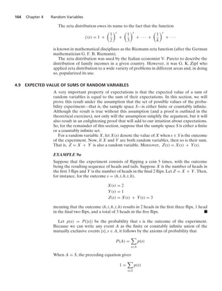
180. Section 4.9 Expected Value of Sums of Random Variables 165
Now, let X be a random variable, and consider E[X]. Because X(s) is the value of X
when s is the outcome of the experiment, it seems intuitive that E[X]—the weighted
average of the possible values of X, with each value weighted by the probability that
X assumes that value—should equal a weighted average of the values X(s), s ∈ S,
with X(s) weighted by the probability that s is the outcome of the experiment. We
now prove this intuition.
Proposition 9.1.
E[X] =
s∈S
X(s) p(s)
Proof. Suppose that the distinct values of X are xi, i Ú 1. For each i, let Si be the
event that X is equal to xi. That is, Si = {s : X(s) = xi}. Then,
E[X] =
i
xiP{X = xi}
=
i
xiP(Si)
=
i
xi
s∈Si
p(s)
=
i
s∈Si
xip(s)
=
i
s∈Si
X(s)p(s)
=
s∈S
X(s)p(s)
where the final equality follows because S1, S2, ... are mutually exclusive events
whose union is S.
EXAMPLE 9b
Suppose that two independent flips of a coin that comes up heads with probability p
are made, and let X denote the number of heads obtained. Because
P(X = 0) = P(t, t) = (1 − p)2
,
P(X = 1) = P(h, t) + P(t, h) = 2p(1 − p)
P(X = 2) = P(h, h) = p2
it follows from the definition of expected value that
E[X] = 0 · (1 − p)2
+ 1 · 2p(1 − p) + 2 · p2
= 2p
which agrees with
E[X] = X(h, h)p2
+ X(h, t)p(1 − p) + X(t, h)(1 − p)p + X(t, t)(1 − p)2
= 2p2
+ p(1 − p) + (1 − p)p
= 2p .
We now prove the important and useful result that the expected value of a sum of
random variables is equal to the sum of their expectations.

181. 166 Chapter 4 Random Variables
Corollary 9.2. For random variables X1, X2, ... , Xn,
E
⎡
⎣
n
i=1
Xi
⎤
⎦ =
n
i=1
E[Xi]
Proof. Let Z = n
i=1 Xi. Then, by Proposition 9.1,
E[Z] =
s∈S
Z(s)p(s)
=
s∈S
X1(s) + X2(s) + ... + Xn(s)
p(s)
=
s∈S
X1(s)p(s) +
s∈S
X2(s)p(s) + ... +
s∈S
Xn(s)p(s)
= E[X1] + E[X2] + ... + E[Xn] .
EXAMPLE 9c
Find the expected value of the sum obtained when n fair dice are rolled.
Solution. Let X be the sum. We will compute E[X] by using the representation
X =
n
i=1
Xi
where Xi is the upturned value on die i. Because Xi is equally likely to be any of the
values from 1 to 6, it follows that
E[Xi] =
6
i=1
i(1/6) = 21/6 = 7/2
which yields the result
E[X] = E
⎡
⎣
n
i=1
Xi
⎤
⎦ =
n
i=1
E[Xi] = 3.5 n
.
EXAMPLE 9d
Find the expected total number of successes that result from n trials when trial i is a
success with probability pi, i = 1, ... , n.
Solution. Letting
Xi =
%
1, if trial i is a success
0, if trial i is a failure
we have the representation
X =
n
i=1
Xi

182. Section 4.9 Expected Value of Sums of Random Variables 167
Consequently,
E[X] =
n
i=1
E[Xi] =
n
i=1
pi
Note that this result does not require that the trials be independent. It includes as a
special case the expected value of a binomial random variable, which assumes inde-
pendent trials and all pi = p, and thus has mean np. It also gives the expected value
of a hypergeometric random variable representing the number of white balls selected
when n balls are randomly selected, without replacement, from an urn of N balls of
which m are white. We can interpret the hypergeometric as representing the number
of successes in n trials, where trial i is said to be a success if the ith ball selected is
white. Because the ith ball selected is equally likely to be any of the N balls and thus
has probability m/N of being white, it follows that the hypergeometric is the num-
ber of successes in n trials in which each trial is a success with probability p = m/N.
Hence, even though these hypergeometric trials are dependent, it follows from the
result of Example 9d that the expected value of the hypergeometric is np = nm/N. .
EXAMPLE 9e
Derive an expression for the variance of the number of successful trials in Example
9d, and apply it to obtain the variance of a binomial random variable with parameters
n and p, and of a hypergeometric random variable equal to the number of white balls
chosen when n balls are randomly chosen from an urn containing N balls of which m
are white.
Solution. Letting X be the number of successful trials, and using the same represen-
tation for X—namely, X = n
i=1 Xi—as in the previous example, we have
E[X2
] = E
⎡
⎢
⎢
⎣
⎛
⎝
n
i=1
Xi
⎞
⎠
⎛
⎜
⎝
n
j=1
Xj
⎞
⎟
⎠
⎤
⎥
⎥
⎦
= E
⎡
⎢
⎣
n
i=1
Xi
⎛
⎝Xi +
jZi
Xj
⎞
⎠
⎤
⎥
⎦
= E
⎡
⎣
n
i=1
X2
i +
n
i=1
jZi
XiXj
⎤
⎦
=
n
i=1
E[X2
i ] +
n
i=1
jZi
E[XiXj]
=
i
pi +
n
i=1
jZi
E[XiXj] (9.1)
where the final equation used that X2
i = Xi. However, because the possible values of
both Xi and Xj are 0 or 1, it follows that
XiXj =
%
1, if Xi = 1, Xj = 1
0, otherwise

183. 168 Chapter 4 Random Variables
Hence,
E[XiXj] = P{Xi = 1, Xj = 1} = P(trials i and j are successes)
Now, on the one hand, if X is binomial, then, for i Z j, the results of trial i and trial j
are independent, with each being a success with probability p. Therefore,
E[XiXj] = p2
, i Z j
Together with Equation (9.1), the preceding equation shows that, for a binomial ran-
dom variable X,
E[X2
] = np + n(n − 1)p2
implying that
Var(X) = E[X2
] − (E[X])2
= np + n(n − 1)p2
− n2
p2
= np(1 − p)
On the other hand, if X is hypergeometric, then, given that a white ball is chosen
in trial i, each of the other N − 1 balls, of which m − 1 are white, is equally likely to
be the jth ball chosen, for j Z i. Consequently, for j Z i,
P{Xi = 1, Xj = 1} = P{Xi = 1}P{Xj = 1|Xi = 1} =
m
N
m − 1
N − 1
Using pi = m/N, we now obtain, from Equation (9.1),
E[X2
] =
nm
N
+ n(n − 1)
m
N
m − 1
N − 1
Consequently,
Var(X) =
nm
N
+ n(n − 1)
m
N
m − 1
N − 1
−
nm
N
2
which, as shown in Example 8j, can be simplified to yield
Var(X) = np(1 − p)
1 −
n − 1
N − 1
where p = m/N. .
4.10 PROPERTIES OF THE CUMULATIVE DISTRIBUTION FUNCTION
Recall that, for the distribution function F of X, F(b) denotes the probability that the
random variable X takes on a value that is less than or equal to b. Following are some
properties of the cumulative distribution function (c.d.f.) F:
1. F is a nondecreasing function; that is, if a b, then F(a) … F(b).
2. lim
b→q
F(b) = 1.
3. lim
b→−q
F(b) = 0.
4. F is right continuous. That is, for any b and any decreasing sequence bn, n Ú 1,
that converges to b, lim
n→q
F(bn) = F(b).
Property 1 follows, as was noted in Section 4.1, because, for a b, the event
{X … a} is contained in the event {X … b} and so cannot have a larger probabil-
ity. Properties 2, 3, and 4 all follow from the continuity property of probabilities

184. Section 4.10 Properties of the Cumulative Distribution Function 169
(Section 2.6). For instance, to prove property 2, we note that if bn increases to q, then
the events {X … bn}, n Ú 1, are increasing events whose union is the event {X q}.
Hence, by the continuity property of probabilities,
lim
n→q
P{X … bn} = P{X q} = 1
which proves property 2.
The proof of property 3 is similar and is left as an exercise. To prove property 4,
we note that if bn decreases to b, then {X … bn}, n Ú 1, are decreasing events whose
intersection is {X … b}. The continuity property then, yields
lim
n
P{X … bn} = P{X … b}
which verifies property 4.
All probability questions about X can be answered in terms of the c.d.f., F. For
example,
P{a X … b} = F(b) − F(a) for all a b (8.1)
This equation can best be seen to hold if we write the event {X … b} as the union of
the mutually exclusive events {X … a} and {a X … b}. That is,
{X … b} = {X … a} ∪ {a X … b}
so
P{X … b} = P{X … a} + P{a X … b}
which establishes Equation (9.1).
If we want to compute the probability that X is strictly less than b, we can again
apply the continuity property to obtain
P{X b} = P
lim
n→q
%
X … b −
1
n
/
= lim
n→q
P
X … b −
1
n
= lim
n→q
F
b −
1
n
Note that P{X b} does not necessarily equal F(b), since F(b) also includes the
probability that X equals b.
EXAMPLE 10a
The distribution function of the random variable X is given by
F(x) =
⎧
⎪
⎪
⎪
⎪
⎪
⎪
⎪
⎪
⎪
⎪
⎪
⎪
⎨
⎪
⎪
⎪
⎪
⎪
⎪
⎪
⎪
⎪
⎪
⎪
⎪
⎩
0 x 0
x
2
0 … x 1
2
3
1 … x 2
11
12
2 … x 3
1 3 … x

185. 170 Chapter 4 Random Variables
1
–
2
2
–
3
1
11
—
12
1 2 3
x
F(x)
FIGURE 4.8: Graph of F(x).
A graph of F(x) is presented in Figure 4.8. Compute (a) P{X 3}, (b) P{X = 1}, (c)
P{X 1
2 }, and (d) P{2 X … 4}.
Solution. (a) P{X 3} = lim
n
P
%
X … 3 −
1
n
/
= lim
n
F
3 −
1
n
=
11
12
(b)
P{X = 1} = P{X … 1} − P{X 1}
= F(1) − lim
n
F
1 −
1
n
=
2
3
−
1
2
=
1
6
(c)
P
%
X
1
2
/
= 1 − P
%
X …
1
2
/
= 1 − F
1
2
=
3
4
(d)
P{2 X … 4} = F(4) − F(2)
=
1
12 .
SUMMARY
A real-valued function defined on the outcome of a probability experiment is called
a random variable.
If X is a random variable, then the function F(x) defined by
F(x) = P{X … x}
is called the distribution function of X. All probabilities concerning X can be stated
in terms of F.

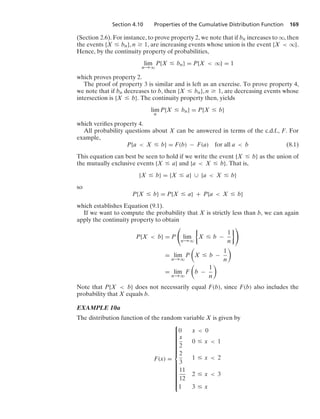
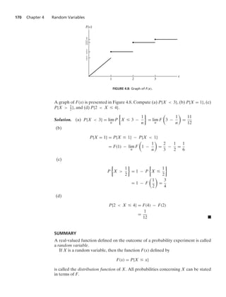
186. Summary 171
A random variable whose set of possible values is either finite or countably infinite
is called discrete. If X is a discrete random variable, then the function
p(x) = P{X = x}
is called the probability mass function of X. Also, the quantity E[X] defined by
E[X] =
x:p(x)0
xp(x)
is called the expected value of X. E[X] is also commonly called the mean or the expec-
tation of X.
A useful identity states that, for a function g,
E[g(X)] =
x:p(x)0
g(x)p(x)
The variance of a random variable X, denoted by Var(X), is defined by
Var(X) = E[(X − E[X])2
]
The variance, which is equal to the expected square of the difference between X
and its expected value, is a measure of the spread of the possible values of X. A useful
identity is
Var(X) = E[X2
] − (E[X])2
The quantity
√
Var(X) is called the standard deviation of X.
We now note some common types of discrete random variables. The random vari-
able X whose probability mass function is given by
p(i) =
n
i
pi
(1 − p)n−i
i = 0, ... , n
is said to be a binomial random variable with parameters n and p. Such a random
variable can be interpreted as being the number of successes that occur when n inde-
pendent trials, each of which results in a success with probability p, are performed.
Its mean and variance are given by
E[X] = np Var(X) = np(1 − p)
The random variable X whose probability mass function is given by
p(i) =
e−λλi
i!
i Ú 0
is said to be a Poisson random variable with parameter λ. If a large number of (approx-
imately) independent trials are performed, each having a small probability of being
successful, then the number of successful trials that result will have a distribution
which is approximately that of a Poisson random variable. The mean and variance of
a Poisson random variable are both equal to its parameter λ. That is,
E[X] = Var(X) = λ
The random variable X whose probability mass function is given by
p(i) = p(1 − p)i−1
i = 1, 2, ...

187. 172 Chapter 4 Random Variables
is said to be a geometric random variable with parameter p. Such a random variable
represents the trial number of the first success when each trial is independently a
success with probability p. Its mean and variance are given by
E[X] =
1
p
Var(X) =
1 − p
p2
The random variable X whose probability mass function is given by
p(i) =
i − 1
r − 1
pr
(1 − p)i−r
i Ú r
is said to be a negative binomial random variable with parameters r and p. Such a
random variable represents the trial number of the rth success when each trial is
independently a success with probability p. Its mean and variance are given by
E[X] =
r
p
Var(X) =
r(1 − p)
p2
A hypergeometric random variable X with parameters n, N, and m represents the
number of white balls selected when n balls are randomly chosen from an urn that
contains N balls of which m are white. The probability mass function of this random
variable is given by
p(i) =
m
i
N − m
n − i
N
n
i = 0, ... , m
With p = m/N, its mean and variance are
E[X] = np Var(X) =
N − n
N − 1
np(1 − p)
An important property of the expected value is that the expected value of a sum of
random variables is equal to the sum of their expected values. That is,
E
⎡
⎣
n
i=1
Xi
⎤
⎦ =
n
i=1
E[Xi]
PROBLEMS
4.1. Two balls are chosen randomly from an urn con-
taining 8 white, 4 black, and 2 orange balls. Sup-
pose that we win $2 for each black ball selected
and we lose $1 for each white ball selected. Let
X denote our winnings. What are the possible val-
ues of X, and what are the probabilities associated
with each value?
4.2. Two fair dice are rolled. Let X equal the
product of the 2 dice. Compute P{X = i} for
i = 1, ... , 36.
4.3. Three dice are rolled. By assuming that each of
the 63 = 216 possible outcomes is equally likely,
find the probabilities attached to the possible val-
ues that X can take on, where X is the sum of
the 3 dice.
4.4. Five men and 5 women are ranked according to
their scores on an examination. Assume that no
two scores are alike and all 10! possible rankings
are equally likely. Let X denote the highest rank-
ing achieved by a woman. (For instance, X = 1

188. Problems 173
if the top-ranked person is female.) Find P{X = i},
i = 1, 2, 3, ... , 8, 9, 10.
4.5. Let X represent the difference between the num-
ber of heads and the number of tails obtained
when a coin is tossed n times. What are the pos-
sible values of X?
4.6. In Problem 5, for n = 3, if the coin is assumed fair,
what are the probabilities associated with the val-
ues that X can take on?
4.7. Suppose that a die is rolled twice. What are the
possible values that the following random vari-
ables can take on:
(a) the maximum value to appear in the two rolls;
(b) the minimum value to appear in the two rolls;
(c) the sum of the two rolls;
(d) the value of the first roll minus the value of
the second roll?
4.8. If the die in Problem 7 is assumed fair, calculate
the probabilities associated with the random vari-
ables in parts (a) through (d).
4.9. Repeat Example 1b when the balls are selected
with replacement.
4.10. In Example 1d, compute the conditional probabil-
ity that we win i dollars, given that we win some-
thing; compute it for i = 1, 2, 3.
4.11. (a) An integer N is to be selected at random from
{1, 2, ... , (10)3} in the sense that each integer
has the same probability of being selected.
What is the probability that N will be divis-
ible by 3? by 5? by 7? by 15? by 105? How
would your answer change if (10)3 is replaced
by (10)k as k became larger and larger?
(b) An important function in number theory—
one whose properties can be shown to be
related to what is probably the most impor-
tant unsolved problem of mathematics, the
Riemann hypothesis—is the Möbius function
μ(n), defined for all positive integral values n
as follows: Factor n into its prime factors. If
there is a repeated prime factor, as in 12 =
2 · 2 · 3 or 49 = 7 · 7, then μ(n) is defined
to equal 0. Now let N be chosen at random
from {1, 2, ... (10)k}, where k is large. Deter-
mine P{μ(N) = 0} as k→q.
Hint: To compute P{μ(N) Z 0}, use the identity
q
i=1
P2
i − 1
P2
i
=
3
4
8
9
24
25
48
49
· · · =
6
π2
where Pi is the ith-smallest prime. (The number 1
is not a prime.)
4.12. In the game of Two-Finger Morra, 2 players show
1 or 2 fingers and simultaneously guess the number
of fingers their opponent will show. If only one of
the players guesses correctly, he wins an amount
(in dollars) equal to the sum of the fingers shown
by him and his opponent. If both players guess
correctly or if neither guesses correctly, then no
money is exchanged. Consider a specified player,
and denote by X the amount of money he wins in
a single game of Two-Finger Morra.
(a) If each player acts independently of the other,
and if each player makes his choice of the
number of fingers he will hold up and the
number he will guess that his opponent will
hold up in such a way that each of the 4 pos-
sibilities is equally likely, what are the possi-
ble values of X and what are their associated
probabilities?
(b) Suppose that each player acts independently
of the other. If each player decides to hold up
the same number of fingers that he guesses his
opponent will hold up, and if each player is
equally likely to hold up 1 or 2 fingers, what
are the possible values of X and their associ-
ated probabilities?
4.13. A salesman has scheduled two appointments to
sell encyclopedias. His first appointment will lead
to a sale with probability .3, and his second will
lead independently to a sale with probability .6.
Any sale made is equally likely to be either for the
deluxe model, which costs $1000, or the standard
model, which costs $500. Determine the probabil-
ity mass function of X, the total dollar value of all
sales.
4.14. Five distinct numbers are randomly distributed
to players numbered 1 through 5. Whenever two
players compare their numbers, the one with the
higher one is declared the winner. Initially, players
1 and 2 compare their numbers; the winner then
compares her number with that of player 3, and so
on. Let X denote the number of times player 1 is a
winner. Find P{X = i}, i = 0, 1, 2, 3, 4.
4.15. The National Basketball Association (NBA) draft
lottery involves the 11 teams that had the worst
won–lost records during the year. A total of 66
balls are placed in an urn. Each of these balls is
inscribed with the name of a team: Eleven have
the name of the team with the worst record, 10
have the name of the team with the second-worst
record, 9 have the name of the team with the third-
worst record, and so on (with 1 ball having the
name of the team with the 11th-worst record).
A ball is then chosen at random, and the team
whose name is on the ball is given the first pick
in the draft of players about to enter the league.
Another ball is then chosen, and if it “belongs”
to a team different from the one that received the
first draft pick, then the team to which it belongs
receives the second draft pick. (If the ball belongs

189. 174 Chapter 4 Random Variables
to the team receiving the first pick, then it is dis-
carded and another one is chosen; this continues
until the ball of another team is chosen.) Finally,
another ball is chosen, and the team named on
the ball (provided that it is different from the
previous two teams) receives the third draft pick.
The remaining draft picks 4 through 11 are then
awarded to the 8 teams that did not “win the lot-
tery,” in inverse order of their won–lost records.
For instance, if the team with the worst record did
not receive any of the 3 lottery picks, then that
team would receive the fourth draft pick. Let X
denote the draft pick of the team with the worst
record. Find the probability mass function of X.
4.16. In Problem 15, let team number 1 be the team
with the worst record, let team number 2 be the
team with the second-worst record, and so on. Let
Yi denote the team that gets draft pick number i.
(Thus, Y1 = 3 if the first ball chosen belongs to
team number 3.) Find the probability mass func-
tion of (a) Y1, (b) Y2, and (c) Y3.
4.17. Suppose that the distribution function of X is
given by
F(b) =
⎧
⎪
⎪
⎪
⎪
⎪
⎪
⎪
⎪
⎪
⎪
⎪
⎪
⎪
⎨
⎪
⎪
⎪
⎪
⎪
⎪
⎪
⎪
⎪
⎪
⎪
⎪
⎪
⎩
0 b 0
b
4
0 … b 1
1
2
+
b − 1
4
1 … b 2
11
12
2 … b 3
1 3 … b
(a) Find P{X = i}, i = 1, 2, 3.
(b) Find P{1
2 X 3
2 }.
4.18. Four independent flips of a fair coin are made. Let
X denote the number of heads obtained. Plot the
probability mass function of the random variable
X − 2.
4.19. If the distribution function of X is given by
F(b) =
⎧
⎪
⎪
⎪
⎪
⎪
⎪
⎪
⎪
⎪
⎪
⎪
⎪
⎪
⎪
⎪
⎪
⎪
⎨
⎪
⎪
⎪
⎪
⎪
⎪
⎪
⎪
⎪
⎪
⎪
⎪
⎪
⎪
⎪
⎪
⎪
⎩
0 b 0
1
2
0 … b 1
3
5
1 … b 2
4
5
2 … b 3
9
10
3 … b 3.5
1 b Ú 3.5
calculate the probability mass function of X.
4.20. A gambling book recommends the following “win-
ning strategy” for the game of roulette: Bet $1 on
red. If red appears
which has probability 18
38
, then
take the $1 profit and quit. If red does not appear
and you lose this bet
which has probability 20
38 of
occurring
, make additional $1 bets on red on each
of the next two spins of the roulette wheel and then
quit. Let X denote your winnings when you quit.
(a) Find P{X 0}.
(b) Are you convinced that the strategy is indeed
a “winning” strategy? Explain your answer!
(c) Find E[X].
4.21. Four buses carrying 148 students from the same
school arrive at a football stadium. The buses
carry, respectively, 40, 33, 25, and 50 students. One
of the students is randomly selected. Let X denote
the number of students that were on the bus car-
rying the randomly selected student. One of the 4
bus drivers is also randomly selected. Let Y denote
the number of students on her bus.
(a) Which of E[X] or E[Y] do you think is larger?
Why?
(b) Compute E[X] and E[Y].
4.22. Suppose that two teams play a series of games that
ends when one of them has won i games. Suppose
that each game played is, independently, won by
team A with probability p. Find the expected num-
ber of games that are played when (a) i = 2 and (b)
i = 3. Also, show in both cases that this number is
maximized when p = 1
2 .
4.23. You have $1000, and a certain commodity
presently sells for $2 per ounce. Suppose that after
one week the commodity will sell for either $1
or $4 an ounce, with these two possibilities being
equally likely.
(a) If your objective is to maximize the expected
amount of money that you possess at the
end of the week, what strategy should you
employ?
(b) If your objective is to maximize the expected
amount of the commodity that you possess at
the end of the week, what strategy should you
employ?
4.24. A and B play the following game: A writes down
either number 1 or number 2, and B must guess
which one. If the number that A has written down
is i and B has guessed correctly, B receives i units
from A. If B makes a wrong guess, B pays 3
4 unit to
A. If B randomizes his decision by guessing 1 with
probability p and 2 with probability 1 − p, deter-
mine his expected gain if (a) A has written down
number 1 and (b) A has written down number 2.
What value of p maximizes the minimum pos-
sible value of B’s expected gain, and what is
this maximin value? (Note that B’s expected

190. Problems 175
gain depends not only on p, but also on what
A does.)
Consider now player A. Suppose that she also
randomizes her decision, writing down number 1
with probability q. What is A’s expected loss if (c)
B chooses number 1 and (d) B chooses number 2?
What value of q minimizes A’s maximum
expected loss? Show that the minimum of A’s max-
imum expected loss is equal to the maximum of B’s
minimum expected gain. This result, known as the
minimax theorem, was first established in general-
ity by the mathematician John von Neumann and
is the fundamental result in the mathematical disci-
pline known as the theory of games. The common
value is called the value of the game to player B.
4.25. Two coins are to be flipped. The first coin will land
on heads with probability .6, the second with prob-
ability .7. Assume that the results of the flips are
independent, and let X equal the total number of
heads that result.
(a) Find P{X = 1}.
(b) Determine E[X].
4.26. One of the numbers 1 through 10 is randomly cho-
sen. You are to try to guess the number chosen by
asking questions with “yes–no” answers. Compute
the expected number of questions you will need to
ask in each of the following two cases:
(a) Your ith question is to be “Is it i?” i =
1, 2, 3, 4, 5, 6, 7, 8, 9, 10.
(b) With each question you try to eliminate one-
half of the remaining numbers, as nearly as
possible.
4.27. An insurance company writes a policy to the effect
that an amount of money A must be paid if some
event E occurs within a year. If the company esti-
mates that E will occur within a year with probabil-
ity p, what should it charge the customer in order
that its expected profit will be 10 percent of A?
4.28. A sample of 3 items is selected at random from a
box containing 20 items of which 4 are defective.
Find the expected number of defective items in the
sample.
4.29. There are two possible causes for a breakdown of
a machine. To check the first possibility would cost
C1 dollars, and, if that were the cause of the break-
down, the trouble could be repaired at a cost of R1
dollars. Similarly, there are costs C2 and R2 asso-
ciated with the second possibility. Let p and 1 −
p denote, respectively, the probabilities that the
breakdown is caused by the first and second possi-
bilities. Under what conditions on p, Ci, Ri, i = 1, 2,
should we check the first possible cause of break-
down and then the second, as opposed to reversing
the checking order, so as to minimize the expected
cost involved in returning the machine to working
order?
Note: If the first check is negative, we must still
check the other possibility.
4.30. A person tosses a fair coin until a tail appears for
the first time. If the tail appears on the nth flip, the
person wins 2n dollars. Let X denote the player’s
winnings. Show that E[X] = +q. This problem is
known as the St. Petersburg paradox.
(a) Would you be willing to pay $1 million to play
this game once?
(b) Would you be willing to pay $1 million for
each game if you could play for as long as
you liked and only had to settle up when you
stopped playing?
4.31. Each night different meteorologists give us the
probability that it will rain the next day. To judge
how well these people predict, we will score each
of them as follows: If a meteorologist says that it
will rain with probability p, then he or she will
receive a score of
1 − (1 − p)2 if it does rain
1 − p2 if it does not rain
We will then keep track of scores over a cer-
tain time span and conclude that the meteorologist
with the highest average score is the best predictor
of weather. Suppose now that a given meteorolo-
gist is aware of our scoring mechanism and wants
to maximize his or her expected score. If this per-
son truly believes that it will rain tomorrow with
probability p∗, what value of p should he or she
assert so as to maximize the expected score?
4.32. To determine whether they have a certain dis-
ease, 100 people are to have their blood tested.
However, rather than testing each individual sepa-
rately, it has been decided first to place the peo-
ple into groups of 10. The blood samples of the
10 people in each group will be pooled and ana-
lyzed together. If the test is negative, one test will
suffice for the 10 people, whereas if the test is posi-
tive, each of the 10 people will also be individually
tested and, in all, 11 tests will be made on this
group. Assume that the probability that a person
has the disease is .1 for all people, independently
of each other, and compute the expected number
of tests necessary for each group. (Note that we are
assuming that the pooled test will be positive if at
least one person in the pool has the disease.)
4.33. A newsboy purchases papers at 10 cents and sells
them at 15 cents. However, he is not allowed to
return unsold papers. If his daily demand is a bino-
mial random variable with n = 10, p = 1
3 , approxi-
mately how many papers should he purchase so as
to maximize his expected profit?
4.34. In Example 4b, suppose that the department store
incurs an additional cost of c for each unit of unmet

191. 176 Chapter 4 Random Variables
demand. (This type of cost is often referred to as
a goodwill cost because the store loses the good-
will of those customers whose demands it can-
not meet.) Compute the expected profit when the
store stocks s units, and determine the value of s
that maximizes the expected profit.
4.35. A box contains 5 red and 5 blue marbles. Two mar-
bles are withdrawn randomly. If they are the same
color, then you win $1.10; if they are different col-
ors, then you win −$1.00. (That is, you lose $1.00.)
Calculate
(a) the expected value of the amount you win;
(b) the variance of the amount you win.
4.36. Consider Problem 22 with i = 2. Find the variance
of the number of games played, and show that this
number is maximized when p = 1
2 .
4.37. Find Var(X) and Var(Y) for X and Y as given in
Problem 21.
4.38. If E[X] = 1 and Var(X) = 5, find
(a) E[(2 + X)2];
(b) Var(4 + 3X).
4.39. A ball is drawn from an urn containing 3 white and
3 black balls. After the ball is drawn, it is replaced
and another ball is drawn. This process goes on
indefinitely. What is the probability that, of the
first 4 balls drawn, exactly 2 are white?
4.40. On a multiple-choice exam with 3 possible answers
for each of the 5 questions, what is the probability
that a student will get 4 or more correct answers
just by guessing?
4.41. A man claims to have extrasensory perception. As
a test, a fair coin is flipped 10 times and the man is
asked to predict the outcome in advance. He gets
7 out of 10 correct. What is the probability that
he would have done at least this well if he had no
ESP?
4.42. Suppose that, in flight, airplane engines will fail
with probability 1 − p, independently from engine
to engine. If an airplane needs a majority of its
engines operative to complete a successful flight,
for what values of p is a 5-engine plane preferable
to a 3-engine plane?
4.43. A communications channel transmits the digits 0
and 1. However, due to static, the digit transmitted
is incorrectly received with probability .2. Suppose
that we want to transmit an important message
consisting of one binary digit. To reduce the
chance of error, we transmit 00000 instead of 0 and
11111 instead of 1. If the receiver of the message
uses “majority” decoding, what is the probability
that the message will be wrong when decoded?
What independence assumptions are you making?
4.44. A satellite system consists of n components and
functions on any given day if at least k of the n
components function on that day. On a rainy day
each of the components independently functions
with probability p1, whereas on a dry day they each
independently function with probability p2. If the
probability of rain tomorrow is α, what is the prob-
ability that the satellite system will function?
4.45. A student is getting ready to take an important
oral examination and is concerned about the pos-
sibility of having an “on” day or an “off” day. He
figures that if he has an on day, then each of his
examiners will pass him, independently of each
other, with probability .8, whereas if he has an off
day, this probability will be reduced to .4. Sup-
pose that the student will pass the examination if a
majority of the examiners pass him. If the student
feels that he is twice as likely to have an off day as
he is to have an on day, should he request an exam-
ination with 3 examiners or with 5 examiners?
4.46. Suppose that it takes at least 9 votes from a 12-
member jury to convict a defendant. Suppose also
that the probability that a juror votes a guilty per-
son innocent is .2, whereas the probability that the
juror votes an innocent person guilty is .1. If each
juror acts independently and if 65 percent of the
defendants are guilty, find the probability that the
jury renders a correct decision. What percentage
of defendants is convicted?
4.47. In some military courts, 9 judges are appointed.
However, both the prosecution and the defense
attorneys are entitled to a peremptory challenge
of any judge, in which case that judge is removed
from the case and is not replaced. A defendant is
declared guilty if the majority of judges cast votes
of guilty, and he or she is declared innocent other-
wise. Suppose that when the defendant is, in fact,
guilty, each judge will (independently) vote guilty
with probability .7, whereas when the defendant is,
in fact, innocent, this probability drops to .3.
(a) What is the probability that a guilty defendant
is declared guilty when there are (i) 9, (ii) 8,
and (iii) 7 judges?
(b) Repeat part (a) for an innocent defendant.
(c) If the prosecution attorney does not exercise
the right to a peremptory challenge of a judge,
and if the defense is limited to at most two
such challenges, how many challenges should
the defense attorney make if he or she is 60
percent certain that the client is guilty?
4.48. It is known that diskettes produced by a cer-
tain company will be defective with probability
.01, independently of each other. The company
sells the diskettes in packages of size 10 and
offers a money-back guarantee that at most 1 of
the 10 diskettes in the package will be defective.
The guarantee is that the customer can return the
entire package of diskettes if he or she finds more

192. Problems 177
than one defective diskette in it. If someone buys
3 packages, what is the probability that he or she
will return exactly 1 of them?
4.49. When coin 1 is flipped, it lands on heads with prob-
ability .4; when coin 2 is flipped, it lands on heads
with probability .7. One of these coins is randomly
chosen and flipped 10 times.
(a) What is the probability that the coin lands on
heads on exactly 7 of the 10 flips?
(b) Given that the first of these ten flips lands
heads, what is the conditional probability that
exactly 7 of the 10 flips land on heads?
4.50. Suppose that a biased coin that lands on heads with
probability p is flipped 10 times. Given that a total
of 6 heads results, find the conditional probability
that the first 3 outcomes are
(a) h, t, t (meaning that the first flip results in
heads, the second in tails, and the third in
tails);
(b) t, h, t.
4.51. The expected number of typographical errors on a
page of a certain magazine is .2. What is the prob-
ability that the next page you read contains (a) 0
and (b) 2 or more typographical errors? Explain
your reasoning!
4.52. The monthly worldwide average number of air-
plane crashes of commercial airlines is 3.5. What
is the probability that there will be
(a) at least 2 such accidents in the next month;
(b) at most 1 accident in the next month?
Explain your reasoning!
4.53. Approximately 80,000 marriages took place in the
state of New York last year. Estimate the proba-
bility that, for at least one of these couples,
(a) both partners were born on April 30;
(b) both partners celebrated their birthday on the
same day of the year.
State your assumptions.
4.54. Suppose that the average number of cars aban-
doned weekly on a certain highway is 2.2. Approx-
imate the probability that there will be
(a) no abandoned cars in the next week;
(b) at least 2 abandoned cars in the next week.
4.55. A certain typing agency employs 2 typists. The
average number of errors per article is 3 when
typed by the first typist and 4.2 when typed by the
second. If your article is equally likely to be typed
by either typist, approximate the probability that it
will have no errors.
4.56. How many people are needed so that the probabil-
ity that at least one of them has the same birthday
as you is greater than 1
2 ?
4.57. Suppose that the number of accidents occurring on
a highway each day is a Poisson random variable
with parameter λ = 3.
(a) Find the probability that 3 or more accidents
occur today.
(b) Repeat part (a) under the assumption that at
least 1 accident occurs today.
4.58. Compare the Poisson approximation with the cor-
rect binomial probability for the following cases:
(a) P{X = 2} when n = 8, p = .1;
(b) P{X = 9} when n = 10, p = .95;
(c) P{X = 0} when n = 10, p = .1;
(d) P{X = 4} when n = 9, p = .2.
4.59. If you buy a lottery ticket in 50 lotteries, in each of
which your chance of winning a prize is 1
100 , what
is the (approximate) probability that you will win
a prize
(a) at least once?
(b) exactly once?
(c) at least twice?
4.60. The number of times that a person contracts a cold
in a given year is a Poisson random variable with
parameter λ = 5. Suppose that a new wonder drug
(based on large quantities of vitamin C) has just
been marketed that reduces the Poisson parame-
ter to λ = 3 for 75 percent of the population. For
the other 25 percent of the population, the drug
has no appreciable effect on colds. If an individ-
ual tries the drug for a year and has 2 colds in that
time, how likely is it that the drug is beneficial for
him or her?
4.61. The probability of being dealt a full house in a
hand of poker is approximately .0014. Find an
approximation for the probability that, in 1000
hands of poker, you will be dealt at least 2 full
houses.
4.62. Consider n independent trials, each of which
results in one of the outcomes 1, ... , k with respec-
tive probabilities p1, ... , pk, k
i=1 pi = 1. Show
that if all the pi are small, then the probability that
no trial outcome occurs more than once is approx-
imately equal to exp(−n(n − 1) i p2
i /2).
4.63. People enter a gambling casino at a rate of 1 every
2 minutes.
(a) What is the probability that no one enters
between 12:00 and 12:05?
(b) What is the probability that at least 4 people
enter the casino during that time?
4.64. The suicide rate in a certain state is 1 suicide per
100,000 inhabitants per month.
(a) Find the probability that, in a city of 400,000
inhabitants within this state, there will be 8 or
more suicides in a given month.

193. 178 Chapter 4 Random Variables
(b) What is the probability that there will be at
least 2 months during the year that will have 8
or more suicides?
(c) Counting the present month as month num-
ber 1, what is the probability that the first
month to have 8 or more suicides will be
month number i, i Ú 1?
What assumptions are you making?
4.65. Each of 500 soldiers in an army company indepen-
dently has a certain disease with probability 1/103.
This disease will show up in a blood test, and to
facilitate matters, blood samples from all 500 sol-
diers are pooled and tested.
(a) What is the (approximate) probability that
the blood test will be positive (that is, at least
one person has the disease)?
Suppose now that the blood test yields a positive
result.
(b) What is the probability, under this circum-
stance, that more than one person has the dis-
ease?
One of the 500 people is Jones, who knows that he
has the disease.
(c) What does Jones think is the probability that
more than one person has the disease?
Because the pooled test was positive, the author-
ities have decided to test each individual sepa-
rately. The first i − 1 of these tests were negative,
and the ith one—which was on Jones—was posi-
tive.
(d) Given the preceding, scenario, what is the
probability, as a function of i, that any of the
remaining people have the disease?
4.66. A total of 2n people, consisting of n married cou-
ples, are randomly seated (all possible orderings
being equally likely) at a round table. Let Ci
denote the event that the members of couple i are
seated next to each other, i = 1, ... , n.
(a) Find P(Ci).
(b) For j Z i, find P(Cj|Ci).
(c) Approximate the probability, for n large, that
there are no married couples who are seated
next to each other.
4.67. Repeat the preceding problem when the seating is
random but subject to the constraint that the men
and women alternate.
4.68. In response to an attack of 10 missiles, 500 antibal-
listic missiles are launched. The missile targets of
the antiballistic missiles are independent, and each
antiballstic missile is equally likely to go towards
any of the target missiles. If each antiballistic mis-
sile independently hits its target with probability
.1, use the Poisson paradigm to approximate the
probability that all missiles are hit.
4.69. A fair coin is flipped 10 times. Find the probability
that there is a string of 4 consecutive heads by
(a) using the formula derived in the text;
(b) using the recursive equations derived in the
text.
(c) Compare your answer with that given by the
Poisson approximation.
4.70. At time 0, a coin that comes up heads with prob-
ability p is flipped and falls to the ground. Sup-
pose it lands on heads. At times chosen accord-
ing to a Poisson process with rate λ, the coin is
picked up and flipped. (Between these times the
coin remains on the ground.) What is the proba-
bility that the coin is on its head side at time t?
Hint What would be the conditional probability
if there were no additional flips by time t, and
what would it be if there were additional flips by
time t?
4.71. Consider a roulette wheel consisting of 38 num-
bers 1 through 36, 0, and double 0. If Smith always
bets that the outcome will be one of the numbers 1
through 12, what is the probability that
(a) Smith will lose his first 5 bets;
(b) his first win will occur on his fourth bet?
4.72. Two athletic teams play a series of games; the first
team to win 4 games is declared the overall win-
ner. Suppose that one of the teams is stronger than
the other and wins each game with probability .6,
independently of the outcomes of the other games.
Find the probability, for i = 4, 5, 6, 7, that the
stronger team wins the series in exactly i games.
Compare the probability that the stronger team
wins with the probability that it would win a 2-out-
of-3 series.
4.73. Suppose in Problem 72 that the two teams are
evenly matched and each has probability 1
2 of win-
ning each game. Find the expected number of
games played.
4.74. An interviewer is given a list of people she can
interview. If the interviewer needs to interview 5
people, and if each person (independently) agrees
to be interviewed with probability 2
3 , what is the
probability that her list of people will enable her
to obtain her necessary number of interviews if
the list consists of (a) 5 people and (b) 8 people?
For part (b), what is the probability that the inter-
viewer will speak to exactly (c) 6 people and (d) 7
people on the list?
4.75. A fair coin is continually flipped until heads
appears for the 10th time. Let X denote the num-
ber of tails that occur. Compute the probability
mass function of X.
4.76. Solve the Banach match problem (Example 8e)
when the left-hand matchbox originally contained

194. Theoretical Exercises 179
N1 matches and the right-hand box contained N2
matches.
4.77. In the Banach matchbox problem, find the prob-
ability that, at the moment when the first box is
emptied (as opposed to being found empty), the
other box contains exactly k matches.
4.78. An urn contains 4 white and 4 black balls. We ran-
domly choose 4 balls. If 2 of them are white and
2 are black, we stop. If not, we replace the balls
in the urn and again randomly select 4 balls. This
continues until exactly 2 of the 4 chosen are white.
What is the probability that we shall make exactly
n selections?
4.79. Suppose that a batch of 100 items contains 6 that
are defective and 94 that are not defective. If X
is the number of defective items in a randomly
drawn sample of 10 items from the batch, find (a)
P{X = 0} and (b) P{X 2}.
4.80. A game popular in Nevada gambling casinos is
Keno, which is played as follows: Twenty num-
bers are selected at random by the casino from the
set of numbers 1 through 80. A player can select
from 1 to 15 numbers; a win occurs if some frac-
tion of the player’s chosen subset matches any of
the 20 numbers drawn by the house. The payoff is a
function of the number of elements in the player’s
selection and the number of matches. For instance,
if the player selects only 1 number, then he or she
wins if this number is among the set of 20, and
the payoff is $2.2 won for every dollar bet. (As
the player’s probability of winning in this case is
1
4 , it is clear that the “fair” payoff should be $3
won for every $1 bet.) When the player selects 2
numbers, a payoff (of odds) of $12 won for every
$1 bet is made when both numbers are among
the 20,
(a) What would be the fair payoff in this case?
Let Pn, k denote the probability that exactly
k of the n numbers chosen by the player are
among the 20 selected by the house.
(b) Compute Pn, k
(c) The most typical wager at Keno consists of
selecting 10 numbers. For such a bet the
casino pays off as shown in the following
table. Compute the expected payoff:
Keno Payoffs in 10 Number Bets
Number of matches Dollars won for each $1 bet
0–4 -1
5 1
6 17
7 179
8 1, 299
9 2, 599
10 24, 999
4.81. In Example 8i, what percentage of i defective lots
does the purchaser reject? Find it for i = 1, 4.
Given that a lot is rejected, what is the condi-
tional probability that it contained 4 defective
components?
4.82. A purchaser of transistors buys them in lots of 20.
It is his policy to randomly inspect 4 components
from a lot and to accept the lot only if all 4 are
nondefective. If each component in a lot is, inde-
pendently, defective with probability .1, what pro-
portion of lots is rejected?
4.83. There are three highways in the county. The num-
ber of daily accidents that occur on these high-
ways are Poisson random variables with respective
parameters .3, .5, and .7. Find the expected num-
ber of accidents that will happen on any of these
highways today.
4.84. Suppose that 10 balls are put into 5 boxes, with
each ball independently being put in box i with
probability pi, 5
i=1 pi = 1.
(a) Find the expected number of boxes that do
not have any balls.
(b) Find the expected number of boxes that have
exactly 1 ball.
4.85. There are k types of coupons. Independently of
the types of previously collected coupons, each
new coupon collected is of type i with probability
pi, k
i=1 pi = 1. If n coupons are collected, find
the expected number of distinct types that appear
in this set. (That is, find the expected number of
types of coupons that appear at least once in the
set of n coupons.)
THEORETICAL EXERCISES
4.1. There are N distinct types of coupons, and each
time one is obtained it will, independently of
past choices, be of type i with probability Pi, i =
1, ... , N. Let T denote the number one need select
to obtain at least one of each type. Compute
P{T = n}.
Hint: Use an argument similar to the one used in
Example 1e.

195. 180 Chapter 4 Random Variables
4.2. If X has distribution function F, what is the distri-
bution function of eX?
4.3. If X has distribution function F, what is the distri-
bution function of the random variable αX + β,
where α and β are constants, α Z 0?
4.4. For a nonnegative integer-valued random vari-
able N, show that
E[N] =
q
i=1
P{N Ú i}
Hint:
q
i=1
P{N Ú i} =
q
i=1
q
k=i
P{N = k}. Now inter-
change the order of summation.
4.5. For a nonnegative integer-valued random variable
N, show that
q
i=0
iP{N i} =
1
2
(E[N2
] − E[N])
Hint:
q
i=0
iP{N i} =
q
i=0
i
q
k=i+1
P{N = k}. Now
interchange the order of summation.
4.6. Let X be such that
P{X = 1} = p = 1 − P{X = −1}
Find c Z 1 such that E[cX] = 1.
4.7. Let X be a random variable having expected value
μ and variance σ2. Find the expected value and
variance of
Y =
X − μ
σ
4.8. Find Var(X) if
P(X = a) = p = 1 − P(X = b)
4.9. Show how the derivation of the binomial probabil-
ities
P{X = i} =
n
i
pi
(1 − p)n−i
, i = 0, ... , n
leads to a proof of the binomial theorem
(x + y)n
=
n
i=0
n
i
xi
yn−i
when x and y are nonnegative.
Hint: Let p = x
x+y .
4.10. Let X be a binomial random variable with param-
eters n and p. Show that
E
1
X + 1
=
1 − (1 − p)n+1
(n + 1)p
4.11. Consider n independent sequential trials, each of
which is successful with probability p. If there
is a total of k successes, show that each of the
n!/[k!(n − k)!] possible arrangements of the k suc-
cesses and n − k failures is equally likely.
4.12. There are n components lined up in a linear
arrangement. Suppose that each component inde-
pendently functions with probability p. What is the
probability that no 2 neighboring components are
both nonfunctional?
Hint: Condition on the number of defective com-
ponents and use the results of Example 4c of
Chapter 1.
4.13. Let X be a binomial random variable with param-
eters (n, p). What value of p maximizes P{X =
k}, k = 0, 1, ... , n? This is an example of a sta-
tistical method used to estimate p when a bino-
mial (n, p) random variable is observed to equal
k. If we assume that n is known, then we estimate
p by choosing that value of p which maximizes
P{X = k}. This is known as the method of maxi-
mum likelihood estimation.
4.14. A family has n children with probability αpn, n Ú 1,
where α … (1 − p)/p.
(a) What proportion of families has no children?
(b) If each child is equally likely to be a boy or a
girl (independently of each other), what pro-
portion of families consists of k boys (and any
number of girls)?
4.15. Suppose that n independent tosses of a coin having
probability p of coming up heads are made. Show
that the probability that an even number of heads
results is 1
2 [1 + (q − p)n], where q = 1 − p. Do
this by proving and then utilizing the identity
[n/2]
i=0
n
2i
p2i
qn−2i
=
1
2
2
(p + q)n
+ (q − p)n
3
where [n/2] is the largest integer less than or equal
to n/2. Compare this exercise with Theoretical
Exercise 3.5 of Chapter 3.
4.16. Let X be a Poisson random variable with parame-
ter λ. Show that P{X = i} increases monotonically
and then decreases monotonically as i increases,
reaching its maximum when i is the largest integer
not exceeding λ.
Hint: Consider P{X = i}/P{X = i − 1}.
4.17. Let X be a Poisson random variable with
parameter λ.
(a) Show that
P{X is even} =
1
2
4
1 + e−2λ
5

196. Theoretical Exercises 181
by using the result of Theoretical Exercise
15 and the relationship between Poisson and
binomial random variables.
(b) Verify the formula in part (a) directly by mak-
ing use of the expansion of e−λ + eλ.
4.18. Let X be a Poisson random variable with parame-
ter λ. What value of λ maximizes P{X = k}, k Ú 0?
4.19. Show that X is a Poisson random variable with
parameter λ, then
E[Xn
] = λE[(X + 1)n−1
]
Now use this result to compute E[X3].
4.20. Consider n coins, each of which independently
comes up heads with probability p. Suppose that
n is large and p is small, and let λ = np. Suppose
that all n coins are tossed; if at least one comes
up heads, the experiment ends; if not, we again
toss all n coins, and so on. That is, we stop the
first time that at least one of the n coins come up
heads. Let X denote the total number of heads that
appear. Which of the following reasonings con-
cerned with approximating P{X = 1} is correct
(in all cases, Y is a Poisson random variable with
parameter λ)?
(a) Because the total number of heads that occur
when all n coins are rolled is approximately a
Poisson random variable with parameter λ,
P{X = 1} L P{Y = 1} = λe−λ
(b) Because the total number of heads that occur
when all n coins are rolled is approximately
a Poisson random variable with parameter λ,
and because we stop only when this number is
positive,
P{X = 1} L P{Y = 1|Y 0} =
λe−λ
1 − e−λ
(c) Because at least one coin comes up heads, X
will equal 1 if none of the other n − 1 coins
come up heads. Because the number of heads
resulting from these n − 1 coins is approxi-
mately Poisson with mean (n − 1)p L λ,
P{X = 1} L P{Y = 0} = e−λ
4.21. From a set of n randomly chosen people, let Eij
denote the event that persons i and j have the same
birthday. Assume that each person is equally likely
to have any of the 365 days of the year as his or her
birthday. Find
(a) P(E3,4|E1,2);
(b) P(E1,3|E1,2);
(c) P(E2,3|E1,2 ∩ E1,3).
What can you conclude from your answers to
parts (a)–(c) about the independence of the
n
2
events Eij?
4.22. An urn contains 2n balls, of which 2 are numbered
1, 2 are numbered 2, ... , and 2 are numbered n.
Balls are successively withdrawn 2 at a time with-
out replacement. Let T denote the first selection
in which the balls withdrawn have the same num-
ber (and let it equal infinity if none of the pairs
withdrawn has the same number). We want to
show that, for 0 α 1,
lim
n
P{T αn} = e−α/2
To verify the preceding formula, let Mk denote the
number of pairs withdrawn in the first k selections,
k = 1, ... , n.
(a) Argue that when n is large, Mk can be
regarded as the number of successes in k
(approximately) independent trials.
(b) Approximate P{Mk = 0} when n is large.
(c) Write the event {T αn} in terms of the value
of one of the variables Mk.
(d) Verify the limiting probability given for
P{T αn}.
4.23. Consider a random collection of n individuals. In
approximating the probability that no 3 of these
individuals share the same birthday, a better Pois-
son approximation than that obtained in the text
(at least for values of n between 80 and 90) is
obtained by letting Ei be the event that there are
at least 3 birthdays on day i, i = 1, ... , 365.
(a) Find P(Ei).
(b) Give an approximation for the probability
that no 3 individuals share the same birthday.
(c) Evaluate the preceding when n = 88 (which
can be shown to be the smallest value of n for
which the probability exceeds .5).
4.24. Here is another way to obtain a set of recur-
sive equations for determining Pn, the probability
that there is a string of k consecutive heads in a
sequence of n flips of a fair coin that comes up
heads with probability p:
(a) Argue that, for k n, there will be a string of
k consecutive heads if either
1. there is a string of k consecutive heads
within the first n − 1 flips, or
2. there is no string of k consecutive heads
within the first n − k − 1 flips, flip n − k
is a tail, and flips n − k + 1, ... , n are
all heads.
(b) Using the preceding, relate Pn to Pn−1. Start-
ing with Pk = pk, the recursion can be used to
obtain Pk+1, then Pk+1, and so on, up to Pn.

197. 182 Chapter 4 Random Variables
4.25. Suppose that the number of events that occur
in a specified time is a Poisson random variable
with parameter λ. If each event is counted with
probability p, independently of every other event,
show that the number of events that are counted
is a Poisson random variable with parameter λp.
Also, give an intuitive argument as to why this
should be so. As an application of the preceding
result, suppose that the number of distinct ura-
nium deposits in a given area is a Poisson random
variable with parameter λ = 10. If, in a fixed
period of time, each deposit is discovered inde-
pendently with probability 1
50 , find the probability
that (a) exactly 1, (b) at least 1, and (c) at most 1
deposit is discovered during that time.
4.26. Prove
n
i=0
e−λ λi
i!
=
1
n!
* q
λ
e−x
xn
dx
Hint: Use integration by parts.
4.27. If X is a geometric random variable, show analyti-
cally that
P{X = n + k|X n} = P{X = k}
Using the interpretation of a geometric random
variable, give a verbal argument as to why the pre-
ceding equation is true.
4.28. Let X be a negative binomial random variable with
parameters r and p, and let Y be a binomial ran-
dom variable with parameters n and p. Show that
P{X n} = P{Y r}
Hint: Either one could attempt an analytical proof
of the preceding equation, which is equivalent to
proving the identity
q
i=n+1
i − 1
r − 1
pr
(1 − p)i−r
=
r−1
i=0
n
i
* pi
(1 − p)n−i
or one could attempt a proof that uses the prob-
abilistic interpretation of these random variables.
That is, in the latter case, start by considering a
sequence of independent trials having a common
probability p of success. Then try to express the
events {X n} and {Y r} in terms of the out-
comes of this sequence.
4.29. For a hypergeometric random variable, determine
P{X = k + 1}/P{X = k}
4.30. Balls numbered 1 through N are in an urn. Sup-
pose that n, n … N, of them are randomly selected
without replacement. Let Y denote the largest
number selected.
(a) Find the probability mass function of Y.
(b) Derive an expression for E[Y] and then use
Fermat’s combinatorial identity (see Theoret-
ical Exercise 11 of Chapter 1) to simplify the
expression.
4.31. A jar contains m + n chips, numbered
1, 2, ... , n + m. A set of size n is drawn. If we
let X denote the number of chips drawn having
numbers that exceed each of the numbers of those
remaining, compute the probability mass function
of X.
4.32. A jar contains n chips. Suppose that a boy succes-
sively draws a chip from the jar, each time replac-
ing the one drawn before drawing another. The
process continues until the boy draws a chip that
he has previously drawn. Let X denote the num-
ber of draws, and compute its probability mass
function.
4.33. Show that Equation (8.6) follows from Equation
(8.5).
4.34. From a set of n elements, a nonempty subset is
chosen at random in the sense that all of the
nonempty subsets are equally likely to be selected.
Let X denote the number of elements in the cho-
sen subset. Using the identities given in Theoreti-
cal Exercise 12 of Chapter 1, show that
E[X] =
n
2 −
1
2
n−1
Var(X) =
n · 22n−2 − n(n + 1)2n−2
(2n − 1)2
Show also that, for n large,
Var(X)
n
4
in the sense that the ratio Var(X) to n/4
approaches 1 as n approaches q. Compare this
formula with the limiting form of Var(Y) when
P{Y = i} = 1/n, i = 1, ... , n.
4.35. An urn initially contains one red and one blue ball.
At each stage, a ball is randomly chosen and then
replaced along with another of the same color. Let
X denote the selection number of the first chosen
ball that is blue. For instance, if the first selec-
tion is red and the second blue, then X is equal
to 2.
(a) Find P{X i}, i Ú 1.
(b) Show that, with probability 1, a blue ball is
eventually chosen. (That is, show that P{X
q} = 1.)
(c) Find E[X].

198. Self-Test Problems and Exercises 183
4.36. Suppose the possible values of X are {xi}, the pos-
sible values of Y are {yj}, and the possible values
of X + Y are {zk}. Let Ak denote the set of all
pairs of indices (i, j) such that xi + yj = zk; that is,
Ak = {(i, j) : xi + yj = zk}.
(a) Argue that
P{X + Y = zk} =
(i,j)∈Ak
P{X = xi, Y = yj}
(b) Show that
E[X + Y] =
k
(i,j)∈Ak
(xi + yj)P{X = xi,
Y = yj}
(c) Using the formula from part (b), argue that
E[X + Y] =
i
j
(xi + yj)P{X = xi,
Y = yj}
(d) Show that
P(X = xi) =
j
P(X = xi, Y = yj),
P(Y = yj) =
i
P{X = xi, Y = yj}
(e) Prove that
E[X + Y] = E[X] + E[Y]
SELF-TEST PROBLEMS AND EXERCISES
4.1. Suppose that the random variable X is equal to
the number of hits obtained by a certain base-
ball player in his next 3 at bats. If P{X = 1} =
.3, P{X = 2} = .2, and P{X = 0} = 3P{X = 3},
find E[X].
4.2. Suppose that X takes on one of the values 0, 1,
and 2. If for some constant c, P{X = i} = cP{X =
i − 1}, i = 1, 2, find E[X].
4.3. A coin that, when flipped, comes up heads with
probability p is flipped until either heads or tails
has occurred twice. Find the expected number of
flips.
4.4. A certain community is composed of m families,
ni of which have i children,
r
i=1
ni = m. If one of
the families is randomly chosen, let X denote the
number of children in that family. If one of the
r
i=1
ini children is randomly chosen, let Y denote
the total number of children in the family of that
child. Show that E[Y] Ú E[X].
4.5. Suppose that P{X = 0} = 1 − P{X = 1}. If
E[X] = 3Var(X), find P{X = 0}.
4.6. There are 2 coins in a bin. When one of them is
flipped, it lands on heads with probability .6, and
when the other is flipped, it lands on heads with
probability .3. One of these coins is to be randomly
chosen and then flipped. Without knowing which
coin is chosen, you can bet any amount up to 10
dollars, and you then either win that amount if the
coin comes up heads or lose it if it comes up tails.
Suppose, however, that an insider is willing to sell
you, for an amount C, the information as to which
coin was selected. What is your expected payoff
if you buy this information? Note that if you buy
it and then bet x, you will end up either winning
x − C or −x − C (that is, losing x + C in the lat-
ter case). Also, for what values of C does it pay to
purchase the information?
4.7. A philanthropist writes a positive number x on a
piece of red paper, shows the paper to an impar-
tial observer, and then turns it face down on the
table. The observer then flips a fair coin. If it shows
heads, she writes the value 2x and, if tails, the value
x/2, on a piece of blue paper, which she then turns
face down on the table. Without knowing either
the value x or the result of the coin flip, you have
the option of turning over either the red or the
blue piece of paper. After doing so and observing
the number written on that paper, you may elect
to receive as a reward either that amount or the
(unknown) amount written on the other piece of
paper. For instance, if you elect to turn over the
blue paper and observe the value 100, then you
can elect either to accept 100 as your reward or
to take the amount (either 200 or 50) on the red
paper. Suppose that you would like your expected
reward to be large.
(a) Argue that there is no reason to turn over the
red paper first, because if you do so, then no
matter what value you observe, it is always
better to switch to the blue paper.
(b) Let y be a fixed nonnegative value, and con-
sider the following strategy: Turn over the
blue paper, and if its value is at least y, then
accept that amount. If it is less than y, then
switch to the red paper. Let Ry(x) denote the
reward obtained if the philanthropist writes
the amount x and you employ this strat-
egy. Find E[Ry(x)]. Note that E[R0(x)] is the

199. 184 Chapter 4 Random Variables
expected reward if the philanthropist writes
the amount x when you employ the strategy
of always choosing the blue paper.
4.8. Let B(n, p) represent a binomial random variable
with parameters n and p. Argue that
P{B(n, p) … i} = 1 − P{B(n, 1 − p) … n − i − 1}
Hint: The number of successes less than or equal to
i is equivalent to what statement about the number
of failures?
4.9. If X is a binomial random variable with expected
value 6 and variance 2.4, find P{X = 5}.
4.10. An urn contains n balls numbered 1 through n. If
you withdraw m balls randomly in sequence, each
time replacing the ball selected previously, find
P{X = k}, k = 1, ... , m, where X is the maximum
of the m chosen numbers.
Hint: First find P{X … k}.
4.11. Teams A and B play a series of games, with the
first team to win 3 games being declared the winner
of the series. Suppose that team A independently
wins each game with probability p. Find the condi-
tional probability that team A wins
(a) the series given that it wins the first game;
(b) the first game given that it wins the series.
4.12. A local soccer team has 5 more games left to play.
If it wins its game this weekend, then it will play
its final 4 games in the upper bracket of its league,
and if it loses, then it will play its final games in
the lower bracket. If it plays in the upper bracket,
then it will independently win each of its games in
this bracket with probability .4, and if it plays in
the lower bracket, then it will independently win
each of its games with probability .7. If the proba-
bility that the team wins its game this weekend is
.5, what is the probability that it wins at least 3 of
its final 4 games?
4.13. Each of the members of a 7-judge panel inde-
pendently makes a correct decision with probabil-
ity .7. If the panel’s decision is made by majority
rule, what is the probability that the panel makes
the correct decision? Given that 4 of the judges
agreed, what is the probability that the panel made
the correct decision?
4.14. On average, 5.2 hurricanes hit a certain region in a
year. What is the probability that there will be 3 or
fewer hurricanes hitting this year?
4.15. The number of eggs laid on a tree leaf by an insect
of a certain type is a Poisson random variable with
parameter λ. However, such a random variable
can be observed only if it is positive, since if it is
0 then we cannot know that such an insect was on
the leaf. If we let Y denote the observed number
of eggs, then
P{Y = i} = P{X = i|X 0}
where X is Poisson with parameter λ. Find E[Y].
4.16. Each of n boys and n girls, independently and ran-
domly, chooses a member of the other sex. If a
boy and girl choose each other, they become a
couple. Number the girls, and let Gi be the event
that girl number i is part of a couple. Let P0 =
1 − P(∪n
i=1Gi) be the probability that no couples
are formed.
(a) What is P(Gi)?
(b) What is P(Gi|Gj)?
(c) When n is large, approximate P0.
(d) When n is large, approximate Pk, the proba-
bility that exactly k couples are formed.
(e) Use the inclusion–exclusion identity to evalu-
ate P0.
4.17. A total of 2n people, consisting of n married cou-
ples, are randomly divided into n pairs. Arbitrarily
number the women, and let Wi denote the event
that woman i is paired with her husband.
(a) Find P(Wi).
(b) For i Z j, find P(Wi|Wj).
(c) When n is large, approximate the probability
that no wife is paired with her husband.
(d) If each pairing must consist of a man and a
woman, what does the problem reduce to?
4.18. A casino patron will continue to make $5 bets on
red in roulette until she has won 4 of these bets.
(a) What is the probability that she places a total
of 9 bets?
(b) What is her expected winnings when she
stops?
Remark: On each bet, she will either win $5 with
probability 18
38 or lose $5 with probability 20
38 .
4.19. When three friends go for coffee, they decide who
will pay the check by each flipping a coin and then
letting the “odd person” pay. If all three flips pro-
duce the same result (so that there is no odd per-
son), then they make a second round of flips, and
they continue to do so until there is an odd person.
What is the probability that
(a) exactly 3 rounds of flips are made?
(b) more than 4 rounds are needed?
4.20. Show that if X is a geometric random variable with
parameter p, then
E[1/X] =
−p log(p)
1 − p
Hint: You will need to evaluate an expression of
the form
q
i=1
ai/i. To do so, write ai/i =
- a
0 xi−1dx,
and then interchange the sum and the integral.
4.21. Suppose that
P{X = a} = p, P{X = b} = 1 − p

200. Self-Test Problems and Exercises 185
(a) Show that X−b
a−b is a Bernoulli random vari-
able.
(b) Find Var(X).
4.22. Each game you play is a win with probability p.
You plan to play 5 games, but if you win the fifth
game, then you will keep on playing until you
lose.
(a) Find the expected number of games that
you play.
(b) Find the expected number of games that
you lose.
4.23. Balls are randomly withdrawn, one at a time with-
out replacement, from an urn that initially has
N white and M black balls. Find the probability
that n white balls are drawn before m black balls,
n … N, m … M.
4.24. Ten balls are to be distributed among 5 urns,
with each ball going into urn i with probabil-
ity pi, 5
i=1 pi = 1. Let Xi denote the number of
balls that go into urn i. Assume that events cor-
responding to the locations of different balls are
independent.
(a) What type of random variable is Xi? Be as
specific as possible.
(b) For i Z j, what type of random variable is
Xi + Xj?
(c) Find P{X1 + X2 + X3 = 7}.
4.25. For the match problem (Example 5m in
Chapter 2), find
(a) the expected number of matches.
(b) the variance of the number of matches.
4.26. Let α be the probability that a geometric random
variable X with parameter p is an even number.
(a) Find α by using the identity α = q
i=1
P{X = 2i}.
(b) Find α by conditioning on whether X = 1 or
X 1.

201. C H A P T E R 5
Continuous Random Variables
5.1 INTRODUCTION
5.2 EXPECTATION AND VARIANCE OF CONTINUOUS RANDOM VARIABLES
5.3 THE UNIFORM RANDOM VARIABLE
5.4 NORMAL RANDOM VARIABLES
5.5 EXPONENTIAL RANDOM VARIABLES
5.6 OTHER CONTINUOUS DISTRIBUTIONS
5.7 THE DISTRIBUTION OF A FUNCTION OF A RANDOM VARIABLE
5.1 INTRODUCTION
In Chapter 4, we considered discrete random variables—that is, random variables
whose set of possible values is either finite or countably infinite. However, there also
exist random variables whose set of possible values is uncountable. Two examples are
the time that a train arrives at a specified stop and the lifetime of a transistor. Let X
be such a random variable. We say that X is a continuous† random variable if there
exists a nonnegative function f, defined for all real x ∈ (−q, q), having the property
that, for any set B of real numbers,‡
P{X ∈ B} =
*
B
f(x) dx (1.1)
The function f is called the probability density function of the random variable X.
(See Figure 5.1.)
In words, Equation (1.1) states that the probability that X will be in B may be
obtained by integrating the probability density function over the set B. Since X must
assume some value, f must satisfy
1 = P{X ∈ (−q, q)} =
* q
−q
f(x) dx
All probability statements about X can be answered in terms of f. For instance, from
Equation (1.1), letting B = [a, b], we obtain
P{a … X … b} =
* b
a
f(x) dx (1.2)
†Sometimes called absolutely continuous.
‡Actually, for technical reasons Equation (1.1) is true only for the measurable sets B, which,
fortunately, include all sets of practical interest.
186

202. Section 5.1 Introduction 187
x
b
a
f
P(a ⱕ X ⱕ b) = area of shaded region
FIGURE 5.1: Probability density function f.
If we let a = b in Equation (1.2), we get
P{X = a} =
* a
a
f(x) dx = 0
In words, this equation states that the probability that a continuous random variable
will assume any fixed value is zero. Hence, for a continuous random variable,
P{X a} = P{X … a} = F(a) =
* a
−q
f(x) dx
EXAMPLE 1a
Suppose that X is a continuous random variable whose probability density function
is given by
f(x) =
0
C(4x − 2x2) 0 x 2
0 otherwise
(a) What is the value of C?
(b) Find P{X 1}.
Solution. (a) Since f is a probability density function, we must have
- q
−q f(x) dx = 1,
implying that
C
* 2
0
(4x − 2x2
) dx = 1
or
C
2x2
−
2x3
3
6
6
6
6
6
x=2
x=0
= 1
or
C =
3
8
Hence,
(b) P{X 1} =
- q
1 f(x) dx = 3
8
- 2
1 (4x − 2x2) dx = 1
2 .

203. 188 Chapter 5 Continuous Random Variables
EXAMPLE 1b
The amount of time in hours that a computer functions before breaking down is a
continuous random variable with probability density function given by
f(x) =
0
λe−x/100 x Ú 0
0 x 0
What is the probability that
(a) a computer will function between 50 and 150 hours before breaking down?
(b) it will function for fewer than 100 hours?
Solution. (a) Since
1 =
* q
−q
f(x) dx = λ
* q
0
e−x/100
dx
we obtain
1 = −λ(100)e−x/100
6
6q
0
= 100λ or λ =
1
100
Hence, the probability that a computer will function between 50 and 150 hours before
breaking down is given by
P{50 X 150} =
* 150
50
1
100
e−x/100
dx = −e−x/100
6
6150
50
= e−1/2
− e−3/2
L .384
(b) Similarly,
P{X 100} =
* 100
0
1
100
e−x/100
dx = −e−x/100
6
6100
0
= 1 − e−1
L .633
In other words, approximately 63.3 percent of the time, a computer will fail before
registering 100 hours of use. .
EXAMPLE 1c
The lifetime in hours of a certain kind of radio tube is a random variable having a
probability density function given by
f(x) =
⎧
⎪
⎨
⎪
⎩
0 x … 100
100
x2
x 100
What is the probability that exactly 2 of 5 such tubes in a radio set will have to be
replaced within the first 150 hours of operation? Assume that the events Ei, i =
1, 2, 3, 4, 5, that the ith such tube will have to be replaced within this time are
independent.

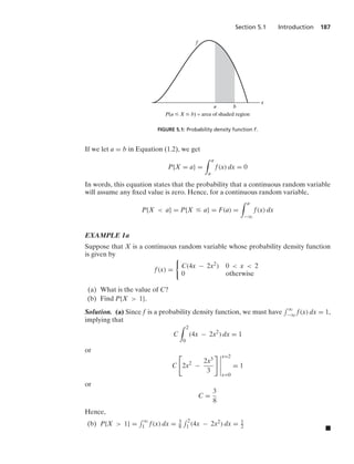
204. Section 5.1 Introduction 189
Solution. From the statement of the problem, we have
P(Ei) =
* 150
0
f(x) dx
= 100
* 150
100
x−2
dx
=
1
3
Hence, from the independence of the events Ei, it follows that the desired probabil-
ity is
5
2
1
3
2
2
3
3
=
80
243 .
The relationship between the cumulative distribution F and the probability density
f is expressed by
F(a) = P{X ∈ (−q, a]} =
* a
−q
f(x) dx
Differentiating both sides of the preceding equation yields
d
da
F(a) = f(a)
That is, the density is the derivative of the cumulative distribution function. A some-
what more intuitive interpretation of the density function may be obtained from
Equation (1.2) as follows:
P
%
a −
ε
2
… X … a +
ε
2
/
=
* a+ε/2
a−ε/2
f(x) dx L εf(a)
when ε is small and when f(·) is continuous at x = a. In other words, the probability
that X will be contained in an interval of length ε around the point a is approximately
εf(a). From this result we see that f(a) is a measure of how likely it is that the random
variable will be near a.
EXAMPLE 1d
If X is continuous with distribution function FX and density function fX, find the
density function of Y = 2X.
Solution. We will determine fY in two ways. The first way is to derive, and then
differentiate, the distribution function of Y:
FY(a) = P{Y … a}
= P{2X … a}
= P{X … a/2}
= FX(a/2)
Differentiation gives
fY(a) =
1
2
fX(a/2)

205. 190 Chapter 5 Continuous Random Variables
Another way to determine fY is to note that
fY(a) L P{a −
2
… Y … a +
2
}
= P{a −
2
… 2X … a +
2
}
= P{
a
2
−
4
… X …
a
2
+
4
}
L
2
fX(a/2)
Dividing through by gives the same result as before. .
5.2 EXPECTATION AND VARIANCE OF CONTINUOUS RANDOM VARIABLES
In Chapter 4, we defined the expected value of a discrete random variable X by
E[X] =
x
xP{X = x}
If X is a continuous random variable having probability density function f(x), then,
because
f(x) dx L P{x … X … x + dx} for dx small
it is easy to see that the analogous definition is to define the expected value of X by
E[X] =
* q
−q
xf(x) dx
EXAMPLE 2a
Find E[X] when the density function of X is
f(x) =
%
2x if 0 … x … 1
0 otherwise
Solution.
E[X] =
*
xf(x) dx
=
* 1
0
2x2
dx
=
2
3 .
EXAMPLE 2b
The density function of X is given by
f(x) =
%
1 if 0 … x … 1
0 otherwise
Find E[eX].

206. Section 5.2 Expectation and Variance of Continuous Random Variables 191
Solution. Let Y = eX. We start by determining FY, the probability distribution func-
tion of Y. Now, for 1 … x … e,
FY(x) = P{Y … x}
= P{eX
… x}
= P{X … log(x)}
=
* log(x)
0
f(y) dy
= log(x)
By differentiating FY(x), we can conclude that the probability density function of Y
is given by
fY(x) =
1
x
1 … x … e
Hence,
E[eX
] = E[Y] =
* q
−q
xfY(x) dx
=
* e
1
dx
= e − 1
.
Although the method employed in Example 2b to compute the expected value of
a function of X is always applicable, there is, as in the discrete case, an alternative
way of proceeding. The following is a direct analog of Proposition 4.1. of Chapter 4.
Proposition 2.1. If X is a continuous random variable with probability density func-
tion f(x), then, for any real-valued function g,
E[g(X)] =
* q
−q
g(x)f(x) dx
An application of Proposition 2.1 to Example 2b yields
E[eX
] =
* 1
0
ex
dx sincef(x) = 1, 0 x 1
= e − 1
which is in accord with the result obtained in that example.
The proof of Proposition 2.1 is more involved than that of its discrete random
variable analog. We will present such a proof under the provision that the random
variable g(X) is nonnegative. (The general proof, which follows the argument in the
case we present, is indicated in Theoretical Exercises 2 and 3.) We will need the fol-
lowing lemma, which is of independent interest.
Lemma 2.1
For a nonnegative random variable Y,
E[Y] =
* q
0
P{Y y} dy

207. 192 Chapter 5 Continuous Random Variables
Proof. We present a proof when Y is a continuous random variable with probabil-
ity density function fY. We have
* q
0
P{Y y} dy =
* q
0
* q
y
fY(x) dx dy
where we have used the fact that P{Y y} =
- q
y fY(x) dx. Interchanging the order
of integration in the preceding equation yields
* q
0
P{Y y} dy =
* q
0
* x
0
dy
fY(x) dx
=
* q
0
xfY(x) dx
= E[Y] .
Proof of Proposition 2.1. From Lemma 2.1, for any function g for which g(x) Ú 0,
E[g(X)] =
* q
0
P{g(X) y} dy
=
* q
0
*
x:g(x)y
f(x) dx dy
=
*
x:g(x)0
* g(x)
0
dy f(x) dx
=
*
x:g(x)0
g(x)f(x) dx
which completes the proof.
EXAMPLE 2c
A stick of length 1 is split at a point U that is uniformly distributed over (0, 1). Deter-
mine the expected length of the piece that contains the point p, 0 … p … 1.
Solution. Let Lp(U) denote the length of the substick that contains the point p, and
note that
Lp(U) =
%
1 − U U p
U U p
(See Figure 5.2.) Hence, from Proposition 2.1,
E[Lp(U)] =
* 1
0
Lp(u) du
=
* p
0
(1 − u)du +
* 1
p
u du
=
1
2
−
(1 − p)2
2
+
1
2
−
p2
2
=
1
2
+ p(1 − p)

208. Section 5.2 Expectation and Variance of Continuous Random Variables 193
0 U p 1
(a)
0 U
p 1
(b)
1 – U
U
FIGURE 5.2: Substick containing point p: (a) U p; (b) U p.
Since p(1 − p) is maximized when p = 1
2 , it is interesting to note that the expected
length of the substick containing the point p is maximized when p is the midpoint of
the original stick. .
EXAMPLE 2d
Suppose that if you are s minutes early for an appointment, then you incur the cost cs,
and if you are s minutes late, then you incur the cost ks. Suppose also that the travel
time from where you presently are to the location of your appointment is a continuous
random variable having probability density function f. Determine the time at which
you should depart if you want to minimize your expected cost.
Solution. Let X denote the travel time. If you leave t minutes before your appoint-
ment, then your cost—call it Ct(X)—is given by
Ct(X) =
%
c(t − X) ifX … t
k(X − t) ifX Ú t
Therefore,
E[Ct(X)] =
* q
0
Ct(x)f(x) dx
=
* t
0
c(t − x)f(x) dx +
* q
t
k(x − t)f(x) dx
= ct
* t
0
f(x) dx − c
* t
0
xf(x) dx + k
* q
t
xf(x) dx − kt
* q
t
f(x) dx
The value of t that minimizes E[Ct(X)] can now be obtained by calculus. Differentia-
tion yields
d
dt
E[Ct(X)] = ct f(t) + cF(t) − ct f(t) − kt f(t) + kt f(t) − k[1 − F(t)]
= (k + c)F(t) − k
Equating the rightmost side to zero shows that the minimal expected cost is obtained
when you leave t∗ minutes before your appointment, where t∗ satisfies
F(t∗
) =
k
k + c
.
As in Chapter 4, we can use Proposition 2.1 to show the following.
Corollary 2.1. If a and b are constants, then
E[aX + b] = aE[X] + b

209. 194 Chapter 5 Continuous Random Variables
The proof of Corollary 2.1 for a continuous random variable X is the same as the
one given for a discrete random variable. The only modification is that the sum is
replaced by an integral and the probability mass function by a probability density
function.
The variance of a continuous random variable is defined exactly as it is for a dis-
crete random variable, namely, if X is a random variable with expected value μ, then
the variance of X is defined (for any type of random variable) by
Var(X) = E[(X − μ)2
]
The alternative formula,
Var(X) = E[X2
] − (E[X])2
is established in a manner similar to its counterpart in the discrete case.
EXAMPLE 2e
Find Var(X) for X as given in Example 2a.
Solution. We first compute E[X2].
E[X2
] =
* q
−q
x2
f(x) dx
=
* 1
0
2x3
dx
=
1
2
Hence, since E[X] = 2
3 , we obtain
Var(X) =
1
2
−
2
3
2
=
1
18 .
It can be shown that, for constants a and b,
Var(aX + b) = a2
Var(X)
The proof mimics the one given for discrete random variables.
There are several important classes of continuous random variables that appear
frequently in applications of probability; the next few sections are devoted to a study
of some of them.
5.3 THE UNIFORM RANDOM VARIABLE
A random variable is said to be uniformly distributed over the interval (0, 1) if its
probability density function is given by
f(x) =
%
1 0 x 1
0 otherwise
(3.1)
Note that Equation (3.1) is a density function, since f(x) Ú 0 and
- q
−q f(x) dx =
- 1
0 dx = 1. Because f(x) 0 only when x ∈ (0, 1), it follows that X must assume
a value in interval (0, 1). Also, since f(x) is constant for x ∈ (0, 1), X is just as likely to

210. Section 5.3 The Uniform Random Variable 195
␣
a
f(a)
␤
1
——–
–
(a)
␣
a
F(a)
␤
(b)
1
␤ ␣
FIGURE 5.3: Graph of (a) f(a) and (b) F(a) for a uniform (α, β) random variable.
be near any value in (0, 1) as it is to be near any other value. To verify this statement,
note that, for any 0 a b 1,
P{a … X … b} =
* b
a
f(x) dx = b − a
In other words, the probability that X is in any particular subinterval of (0, 1) equals
the length of that subinterval.
In general, we say that X is a uniform random variable on the interval (α, β) if the
probability density function of X is given by
f(x) =
⎧
⎪
⎨
⎪
⎩
1
β − α
if α x β
0 otherwise
(3.2)
Since F(a) =
- a
−q f(x) dx, it follows from Equation (3.2) that the distribution function
of a uniform random variable on the interval (α, β) is given by
F(a) =
⎧
⎪
⎪
⎪
⎨
⎪
⎪
⎪
⎩
0 a … α
a − α
β − α
α a β
1 a Ú β
Figure 5.3 presents a graph of f(a) and F(a).
EXAMPLE 3a
Let X be uniformly distributed over (α, β). Find (a) E[X] and (b) Var(X).
Solution. (a)
E[X] =
* q
−q
xf(x) dx
=
* β
α
x
β − α
dx
=
β2 − α2
2(β − α)
=
β + α
2

211. 196 Chapter 5 Continuous Random Variables
In words, the expected value of a random variable that is uniformly distributed
over some interval is equal to the midpoint of that interval.
(b) To find Var(X), we first calculate E[X2].
E[X2
] =
* β
α
1
β − α
x2
dx
=
β3 − α3
3(β − α)
=
β2 + αβ + α2
3
Hence,
Var(X) =
β2 + αβ + α2
3
−
(α + β)2
4
=
(β − α)2
12
Therefore, the variance of a random variable that is uniformly distributed over
some interval is the square of the length of that interval divided by 12. .
EXAMPLE 3b
If X is uniformly distributed over (0, 10), calculate the probability that (a) X 3, (b)
X 6, and (c) 3 X 8.
Solution. (a) P{X 3} =
* 3
0
1
10
dx =
3
10
(b) P{X 6} =
* 10
6
1
10
dx =
4
10
(c) P{3 X 8} =
* 8
3
1
10
dx =
1
2
.
EXAMPLE 3c
Buses arrive at a specified stop at 15-minute intervals starting at 7 A.M. That is, they
arrive at 7, 7:15, 7:30, 7:45, and so on. If a passenger arrives at the stop at a time that
is uniformly distributed between 7 and 7:30, find the probability that he waits
(a) less than 5 minutes for a bus;
(b) more than 10 minutes for a bus.
Solution. Let X denote the number of minutes past 7 that the passenger arrives at
the stop. Since X is a uniform random variable over the interval (0, 30), it follows that
the passenger will have to wait less than 5 minutes if (and only if) he arrives between
7:10 and 7:15 or between 7:25 and 7:30. Hence, the desired probability for part (a) is
P{10 X 15} + P{25 X 30} =
* 15
10
1
30
dx +
* 30
25
1
30
dx =
1
3
Similarly, he would have to wait more than 10 minutes if he arrives between 7 and
7:05 or between 7:15 and 7:20, so the probability for part (b) is
P{0 X 5} + P{15 X 20} =
1
3
.

212. Section 5.3 The Uniform Random Variable 197
The next example was first considered by the French mathematician Joseph
L. F. Bertrand in 1889 and is often referred to as Bertrand’s paradox. It represents
our initial introduction to a subject commonly referred to as geometrical probability.
EXAMPLE 3d
Consider a random chord of a circle. What is the probability that the length of the
chord will be greater than the side of the equilateral triangle inscribed in that circle?
Solution. As stated, the problem is incapable of solution because it is not clear what
is meant by a random chord. To give meaning to this phrase, we shall reformulate the
problem in two distinct ways.
The first formulation is as follows: The position of the chord can be determined
by its distance from the center of the circle. This distance can vary between 0 and
r, the radius of the circle. Now, the length of the chord will be greater than the side
of the equilateral triangle inscribed in the circle if the distance from the chord to the
center of the circle is less than r/2. Hence, by assuming that a random chord is a chord
whose distance D from the center of the circle is uniformly distributed between 0 and
r, we see that the probability that the length of the chord is greater than the side of
an inscribed equilateral triangle is
P
%
D
r
2
/
=
r/2
r
=
1
2
For our second formulation of the problem, consider an arbitrary chord of the cir-
cle; through one end of the chord, draw a tangent. The angle θ between the chord and
the tangent, which can vary from 0◦ to 180◦, determines the position of the chord. (See
Figure 5.4.) Furthermore, the length of the chord will be greater than the side of the
inscribed equilateral triangle if the angle θ is between 60◦ and 120◦. Hence, assuming
that a random chord is a chord whose angle θ is uniformly distributed between 0◦ and
180◦, we see that the desired answer in this formulation is
P{60 θ 120} =
120 − 60
180
=
1
3
Note that random experiments could be performed in such a way that 1
2 or 1
3 would
be the correct probability. For instance, if a circular disk of radius r is thrown on a
table ruled with parallel lines a distance 2r apart, then one and only one of these lines
would cross the disk and form a chord. All distances from this chord to the center of
the disk would be equally likely, so that the desired probability that the chord’s length
will be greater than the side of an inscribed equilateral triangle is 1
2. In contrast, if the
A
␪
FIGURE 5.4

213. 198 Chapter 5 Continuous Random Variables
experiment consisted of rotating a needle freely about a point A on the edge (see
Figure 5.4) of the circle, the desired answer would be 1
3. .
5.4 NORMAL RANDOM VARIABLES
We say that X is a normal random variable, or simply that X is normally distributed,
with parameters μ and σ2 if the density of X is given by
f(x) =
1
√
2πσ
e−(x−μ)2/2σ2
− q x q
This density function is a bell-shaped curve that is symmetric about μ. (See Figure 5.5.)
(b)
– 2
3
(a)
–3 –2 –1 0 1 2
.399
.399
——–
␴
␮
␴
␮ + 2␴
␮
– ␴
␮ + ␴
␮
FIGURE 5.5: Normal density function: (a) μ = 0, σ = 1; (b) arbitrary μ, σ2.
The normal distribution was introduced by the French mathematician Abraham
DeMoivre in 1733, who used it to approximate probabilities associated with bino-
mial random variables when the binomial parameter n is large. This result was later
extended by Laplace and others and is now encompassed in a probability theorem
known as the central limit theorem, which is discussed in Chapter 8. The central limit
theorem, one of the two most important results in probability theory,† gives a theo-
retical base to the often noted empirical observation that, in practice, many random
phenomena obey, at least approximately, a normal probability distribution. Some
examples of random phenomena obeying this behavior are the height of a man, the
velocity in any direction of a molecule in gas, and the error made in measuring a
physical quantity.
To prove that f(x) is indeed a probability density function, we need to show that
1
√
2πσ
* q
−q
e−(x−μ)2/2σ2
dx = 1
†The other is the strong law of large numbers.

214. Section 5.4 Normal Random Variables 199
Making the substitution y = (x − μ)/σ, we see that
1
√
2πσ
* q
−q
e−(x−μ)2/2σ2
dx =
1
√
2π
* q
−q
e−y2/2
dy
Hence, we must show that * q
−q
e−y2/2
dy =
√
2π
Toward this end, let I =
- q
−q e−y2/2 dy. Then
I2
=
* q
−q
e−y2/2
dy
* q
−q
e−x2/2
dx
=
* q
−q
* q
−q
e−(y2+x2)/2
dy dx
We now evaluate the double integral by means of a change of variables to polar
coordinates. (That is, let x = r cos θ, y = r sin θ, and dy dx = r dθ dr.) Thus,
I2
=
* q
0
* 2π
0
e−r2/2
r dθ dr
= 2π
* q
0
re−r2/2
dr
= −2πe−r2/2
6
6q
0
= 2π
Hence, I =
√
2π, and the result is proved.
An important fact about normal random variables is that if X is normally dis-
tributed with parameters μ and σ2, then Y = aX + b is normally distributed with
parameters aμ + b and a2σ2. To prove this statement, suppose that a 0. (The proof
when a 0 is similar.) Let FY denote the cumulative distribution function of Y. Then
FY(x) = P{Y … x}
= P{aX + b … x}
= P{X …
x − b
a
}
= FX(
x − b
a
)
where FX is the cumulative distribution function of X. By differentiation, the density
function of Y is then
fY(x) =
1
a
fX(
x − b
a
)
=
1
√
2πaσ
exp{−(
x − b
a
− μ)2
/2σ2
}
=
1
√
2πaσ
exp{−(x − b − aμ)2
/2(aσ)2
}
which shows that Y is normal with parameters aμ + b and a2σ2.

215. 200 Chapter 5 Continuous Random Variables
An important implication of the preceding result is that if X is normally distributed
with parameters μ and σ2, then Z = (X − μ)/σ is normally distributed with parame-
ters 0 and 1. Such a random variable is said to be a standard, or a unit, normal random
variable.
We now show that the parameters μ and σ2 of a normal random variable represent,
respectively, its expected value and variance.
EXAMPLE 4a
Find E[X] and Var(X) when X is a normal random variable with parameters μ and σ2.
Solution. Let us start by finding the mean and variance of the standard normal ran-
dom variable Z = (X − μ)/σ. We have
E[Z] =
* q
−q
xfZ(x) dx
=
1
√
2π
* q
−q
xe−x2/2
dx
= −
1
√
2π
e−x2/2
|q
−q
= 0
Thus,
Var(Z) = E[Z2
]
=
1
√
2π
* q
−q
x2
e−x2/2
dx
Integration by parts (with u = x and dv = xe−x2/2) now gives
Var(Z) =
1
√
2π
(−xe−x2/2
|q
−q +
* q
−q
e−x2/2
dx)
=
1
√
2π
* q
−q
e−x2/2
dx
= 1
Because X = μ + σZ, the preceding yields the results
E[X] = μ + σE[Z] = μ
and
Var(X) = σ2
Var(Z) = σ2
.
It is customary to denote the cumulative distribution function of a standard normal
random variable by (x). That is,
(x) =
1
√
2π
* x
−q
e−y2/2
dy
The values of (x) for nonnegative x are given in Table 5.1. For negative values of x,
(x) can be obtained from the relationship
(−x) = 1 − (x) − q x q (4.1)

216. Section 5.4 Normal Random Variables 201
TABLE 5.1: AREA (x) UNDER THE STANDARD NORMAL CURVE TO THE LEFT OF X
X .00 .01 .02 .03 .04 .05 .06 .07 .08 .09
.0 .5000 .5040 .5080 .5120 .5160 .5199 .5239 .5279 .5319 .5359
.1 .5398 .5438 .5478 .5517 .5557 .5596 .5636 .5675 .5714 .5753
.2 .5793 .5832 .5871 .5910 .5948 .5987 .6026 .6064 .6103 .6141
.3 .6179 .6217 .6255 .6293 .6331 .6368 .6406 .6443 .6480 .6517
.4 .6554 .6591 .6628 .6664 .6700 .6736 .6772 .6808 .6844 .6879
.5 .6915 .6950 .6985 .7019 .7054 .7088 .7123 .7157 .7190 .7224
.6 .7257 .7291 .7324 .7357 .7389 .7422 .7454 .7486 .7517 .7549
.7 .7580 .7611 .7642 .7673 .7704 .7734 .7764 .7794 .7823 .7852
.8 .7881 .7910 .7939 .7967 .7995 .8023 .8051 .8078 .8106 .8133
.9 .8159 .8186 .8212 .8238 .8264 .8289 .8315 .8340 .8365 .8389
1.0 .8413 .8438 .8461 .8485 .8508 .8531 .8554 .8577 .8599 .8621
1.1 .8643 .8665 .8686 .8708 .8729 .8749 .8770 .8790 .8810 .8830
1.2 .8849 .8869 .8888 .8907 .8925 .8944 .8962 .8980 .8997 .9015
1.3 .9032 .9049 .9066 .9082 .9099 .9115 .9131 .9147 .9162 .9177
1.4 .9192 .9207 .9222 .9236 .9251 .9265 .9279 .9292 .9306 .9319
1.5 .9332 .9345 .9357 .9370 .9382 .9394 .9406 .9418 .9429 .9441
1.6 .9452 .9463 .9474 .9484 .9495 .9505 .9515 .9525 .9535 .9545
1.7 .9554 .9564 .9573 .9582 .9591 .9599 .9608 .9616 .9625 .9633
1.8 .9641 .9649 .9656 .9664 .9671 .9678 .9686 .9693 .9699 .9706
1.9 .9713 .9719 .9726 .9732 .9738 .9744 .9750 .9756 .9761 .9767
2.0 .9772 .9778 .9783 .9788 .9793 .9798 .9803 .9808 .9812 .9817
2.1 .9821 .9826 .9830 .9834 .9838 .9842 .9846 .9850 .9854 .9857
2.2 .9861 .9864 .9868 .9871 .9875 .9878 .9881 .9884 .9887 .9890
2.3 .9893 .9896 .9898 .9901 .9904 .9906 .9909 .9911 .9913 .9916
2.4 .9918 .9920 .9922 .9925 .9927 .9929 .9931 .9932 .9934 .9936
2.5 .9938 .9940 .9941 .9943 .9945 .9946 .9948 .9949 .9951 .9952
2.6 .9953 .9955 .9956 .9957 .9959 .9960 .9961 .9962 .9963 .9964
2.7 .9965 .9966 .9967 .9968 .9969 .9970 .9971 .9972 .9973 .9974
2.8 .9974 .9975 .9976 .9977 .9977 .9978 .9979 .9979 .9980 .9981
2.9 .9981 .9982 .9982 .9983 .9984 .9984 .9985 .9985 .9986 .9986
3.0 .9987 .9987 .9987 .9988 .9988 .9989 .9989 .9989 .9990 .9990
3.1 .9990 .9991 .9991 .9991 .9992 .9992 .9992 .9992 .9993 .9993
3.2 .9993 .9993 .9994 .9994 .9994 .9994 .9994 .9995 .9995 .9995
3.3 .9995 .9995 .9995 .9996 .9996 .9996 .9996 .9996 .9996 .9997
3.4 .9997 .9997 .9997 .9997 .9997 .9997 .9997 .9997 .9997 .9998
The proof of Equation (4.1), which follows from the symmetry of the standard nor-
mal density, is left as an exercise. This equation states that if Z is a standard normal
random variable, then
P{Z … −x} = P{Z x} − q x q
Since Z = (X − μ)/σ is a standard normal random variable whenever X is normally
distributed with parameters μ and σ2, it follows that the distribution function of X
can be expressed as
FX(a) = P{X … a} = P
X − μ
σ
…
a − μ
σ
=
a − μ
σ

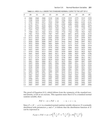
217. 202 Chapter 5 Continuous Random Variables
EXAMPLE 4b
If X is a normal random variable with parameters μ = 3 and σ2 = 9, find (a) P{2
X 5}; (b) P{X 0}; (c) P{|X − 3| 6}.
Solution. (a)
P{2 X 5} = P
%
2 − 3
3
X − 3
3
5 − 3
3
/
= P
%
−
1
3
Z
2
3
/
=
2
3
−
−
1
3
=
2
3
−
1 −
1
3
L .3779
(b)
P{X 0} = P
%
X − 3
3
0 − 3
3
/
= P{Z −1}
= 1 − (−1)
= (1)
L .8413
(c)
P{|X − 3| 6} = P{X 9} + P{X −3}
= P
%
X − 3
3
9 − 3
3
/
+ P
%
X − 3
3
−3 − 3
3
/
= P{Z 2} + P{Z −2}
= 1 − (2) + (−2)
= 2[1 − (2)]
L .0456
.
EXAMPLE 4c
An examination is frequently regarded as being good (in the sense of determining
a valid grade spread for those taking it) if the test scores of those taking the exami-
nation can be approximated by a normal density function. (In other words, a graph
of the frequency of grade scores should have approximately the bell-shaped form of
the normal density.) The instructor often uses the test scores to estimate the normal
parameters μ and σ2 and then assigns the letter grade A to those whose test score
is greater than μ + σ, B to those whose score is between μ and μ + σ, C to those
whose score is between μ − σ and μ, D to those whose score is between μ − 2σ
and μ − σ, and F to those getting a score below μ − 2σ. (This strategy is sometimes
referred to as grading “on the curve.”) Since

218. Section 5.4 Normal Random Variables 203
P{X μ + σ} = P
%
X − μ
σ
1
/
= 1 − (1) L .1587
P{μ X μ + σ} = P
%
0
X − μ
σ
1
/
= (1) − (0) L .3413
P{μ − σ X μ} = P
%
−1
X − μ
σ
0
/
= (0) − (−1) L .3413
P{μ − 2σ X μ − σ} = P
%
−2
X − μ
σ
−1
/
= (2) − (1) L .1359
P{X μ − 2σ} = P
%
X − μ
σ
−2
/
= (−2) L .0228
it follows that approximately 16 percent of the class will receive an A grade on the
examination, 34 percent a B grade, 34 percent a C grade, and 14 percent a D grade; 2
percent will fail. .
EXAMPLE 4d
An expert witness in a paternity suit testifies that the length (in days) of human ges-
tation is approximately normally distributed with parameters μ = 270 and σ2 = 100.
The defendant in the suit is able to prove that he was out of the country during a
period that began 290 days before the birth of the child and ended 240 days before
the birth. If the defendant was, in fact, the father of the child, what is the probability
that the mother could have had the very long or very short gestation indicated by the
testimony?
Solution. Let X denote the length of the gestation, and assume that the defendant
is the father. Then the probability that the birth could occur within the indicated
period is
P{X 290orX 240} = P{X 290} + P{X 240}
= P
%
X − 270
10
2
/
+ P
%
X − 270
10
−3
/
= 1 − (2) + 1 − (3)
L .0241
.
EXAMPLE 4e
Suppose that a binary message—either 0 or 1—must be transmitted by wire from
location A to location B. However, the data sent over the wire are subject to a channel
noise disturbance, so, to reduce the possibility of error, the value 2 is sent over the
wire when the message is 1 and the value −2 is sent when the message is 0. If x, x = ;2,
is the value sent at location A, then R, the value received at location B, is given by
R = x + N, where N is the channel noise disturbance. When the message is received
at location B, the receiver decodes it according to the following rule:
If R Ú .5, then 1 is concluded.
If R .5, then 0 is concluded.

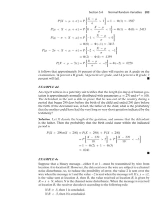
219. 204 Chapter 5 Continuous Random Variables
Because the channel noise is often normally distributed, we will determine the error
probabilities when N is a standard normal random variable.
Two types of errors can occur: One is that the message 1 can be incorrectly deter-
mined to be 0, and the other is that 0 can be incorrectly determined to be 1. The first
type of error will occur if the message is 1 and 2 + N .5, whereas the second will
occur if the message is 0 and −2 + N Ú .5. Hence,
P{error|message is 1} = P{N −1.5}
= 1 − (1.5) L .0668
and
P{error|message is 0} = P{N Ú 2.5}
= 1 − (2.5) L .0062
.
5.4.1 The Normal Approximation to the Binomial Distribution
An important result in probability theory known as the DeMoivre–Laplace limit the-
orem states that when n is large, a binomial random variable with parameters n and p
will have approximately the same distribution as a normal random variable with the
same mean and variance as the binomial. This result was proved originally for the spe-
cial case of p = 1
2 by DeMoivre in 1733 and was then extended to general p by Laplace
in 1812. It formally states that if we “standardize” the binomial by first subtracting its
mean np and then dividing the result by its standard deviation
.
np(1 − p), then the
distribution function of this standardized random variable (which has mean 0 and
variance 1) will converge to the standard normal distribution function as n→q.
The DeMoivre–Laplace limit theorem
If Sn denotes the number of successes that occur when n independent trials, each
resulting in a success with probability p, are performed, then, for any a b,
P
0
a …
Sn − np
.
np(1 − p)
… b
7
→ (b) − (a)
as n→q.
Because the preceding theorem is only a special case of the central limit theorem,
which is presented in Chapter 8, we shall not present a proof.
Note that we now have two possible approximations to binomial probabilities: the
Poisson approximation, which is good when n is large and p is small, and the normal
approximation, which can be shown to be quite good when np(1 − p) is large. (See
Figure 5.6.) [The normal approximation will, in general, be quite good for values of n
satisfying np(1 − p) Ú 10.]
EXAMPLE 4f
Let X be the number of times that a fair coin that is flipped 40 times lands on heads.
Find the probability that X = 20. Use the normal approximation and then compare
it with the exact solution.

220. Section 5.4 Normal Random Variables 205
0 2 4 6
(10, 0.7)
8 10 0
0 5
0.0
0.02
0.04
0.06
0.08
0.10
0.12
0.14
0.16
0.0
0.14
0.12
0.10
0.08
0.06
0.04
0.02
0.0
0.30
0.25
0.20
0.15
0.10
0.05
0.0
0.20
0.15
0.10
0.05
10 15
(30, 0.7)
20 25 30 0 10 20
(50, 0.7)
30 40 50
5 10
(20, 0.7)
x
x x
x
15 20
FIGURE 5.6: The probability mass function of a binomial (n, p) random variable becomes more and more
“normal” as n becomes larger and larger.
Solution. To employ the normal approximation, note that because the binomial is
a discrete integer-valued random variable, whereas the normal is a continuous ran-
dom variable, it is best to write P{X = i} as P{i − 1/2 X i + 1/2} before
applying the normal approximation (this is called the continuity correction). Doing
so gives
P{X = 20} = P{19.5 … X 20.5}
= P
0
19.5 − 20
√
10
X − 20
√
10
20.5 − 20
√
10
7
L P
0
−.16
X − 20
√
10
.16
7
L (.16) − (−.16) L .1272
The exact result is
P{X = 20} =
40
20
1
2
40
L .1254 .
EXAMPLE 4g
The ideal size of a first-year class at a particular college is 150 students. The college,
knowing from past experience that, on the average, only 30 percent of those accepted
for admission will actually attend, uses a policy of approving the applications of 450
students. Compute the probability that more than 150 first-year students attend this
college.
Solution. If X denotes the number of students that attend, then X is a binomial ran-
dom variable with parameters n = 450 and p = .3. Using the continuity correction,

221. 206 Chapter 5 Continuous Random Variables
we see that the normal approximation yields
P{X Ú 150.5} = P
0
X − (450)(.3)
√
450(.3)(.7)
Ú
150.5 − (450)(.3)
√
450(.3)(.7)
7
L 1 − (1.59)
L .0559
Hence, less than 6 percent of the time do more than 150 of the first 450 accepted
actually attend. (What independence assumptions have we made?) .
EXAMPLE 4h
To determine the effectiveness of a certain diet in reducing the amount of cholesterol
in the bloodstream, 100 people are put on the diet. After they have been on the diet
for a sufficient length of time, their cholesterol count will be taken. The nutritionist
running this experiment has decided to endorse the diet if at least 65 percent of the
people have a lower cholesterol count after going on the diet. What is the probability
that the nutritionist endorses the new diet if, in fact, it has no effect on the cholesterol
level?
Solution. Let us assume that if the diet has no effect on the cholesterol count, then,
strictly by chance, each person’s count will be lower than it was before the diet with
probability 1
2 . Hence, if X is the number of people whose count is lowered, then the
probability that the nutritionist will endorse the diet when it actually has no effect on
the cholesterol count is
100
i=65
100
i
1
2
100
= P{X Ú 64.5}
= P
⎧
⎪
⎨
⎪
⎩
X − (100)(1
2)
8
100(1
2)(1
2)
Ú 2.9
⎫
⎪
⎬
⎪
⎭
L 1 − (2.9)
L .0019 .
EXAMPLE 4i
Fifty-two percent of the residents of New York City are in favor of outlawing cigarette
smoking in publicly owned areas. Approximate the probability that more than 50
percent of a random sample of n people from New York are in favor of this prohibi-
tion when
(a) n = 11
(b) n = 101
(c) n = 1001
How large would n have to be to make this probability exceed .95?
Solution. Let N denote the number of residents of New York City. To answer the
preceding question, we must first understand that a random sample of size n is a
sample such that the n people were chosen in such a manner that each of the
N
n
subsets of n people had the same chance of being the chosen subset. Consequently,

222. Section 5.4 Normal Random Variables 207
Sn, the number of people in the sample who are in favor of the smoking prohibition,
is a hypergeometric random variable. That is, Sn has the same distribution as the
number of white balls obtained when n balls are chosen from an urn of N balls, of
which .52N are white. But because N and .52N are both large in comparison with the
sample size n, it follows from the binomial approximation to the hypergeometric (see
Section 4.8.3) that the distribution of Sn is closely approximated by a binomial dis-
tribution with parameters n and p = .52. The normal approximation to the binomial
distribution then shows that
P{Sn .5n} = P
0
Sn − .52n
√
n(.52)(.48)
.5n − .52n
√
n(.52)(.48)
7
= P
0
Sn − .52n
√
n(.52)(.48)
−.04
√
n
7
L (.04
√
n)
Thus,
P{Sn .5n} L
⎧
⎨
⎩
(.1328) = .5528, if n = 11
(.4020) = .6562, if n = 101
(1.2665) = .8973, if n = 1001
In order for this probability to be at least .95, we would need (.04
√
n) .95. Because
(x) is an increasing function and (1.645) = .95, this means that
.04
√
n 1.645
or
n Ú 1691.266
That is, the sample size would have to be at least 1692. .
Historical Notes Concerning the Normal Distribution
The normal distribution was introduced by the French mathematician Abraham
DeMoivre in 1733. DeMoivre, who used this distribution to approximate proba-
bilities connected with coin tossing, called it the exponential bell-shaped curve. Its
usefulness, however, became truly apparent only in 1809, when the famous German
mathematician Karl Friedrich Gauss used it as an integral part of his approach to
predicting the location of astronomical entities. As a result, it became common after
this time to call it the Gaussian distribution.
During the mid- to late 19th century, however, most statisticians started to
believe that the majority of data sets would have histograms conforming to the
Gaussian bell-shaped form. Indeed, it came to be accepted that it was “normal”
for any well-behaved data set to follow this curve. As a result, following the lead of
the British statistician Karl Pearson, people began referring to the Gaussian curve
by calling it simply the normal curve. (A partial explanation as to why so many data
sets conform to the normal curve is provided by the central limit theorem, which is
presented in Chapter 8.)
Abraham DeMoivre (1667–1754)
Today there is no shortage of statistical consultants, many of whom ply their trade
in the most elegant of settings. However, the first of their breed worked, in the early

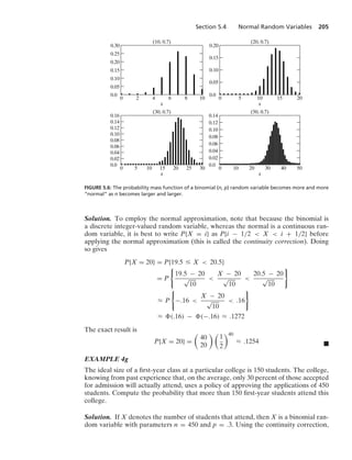
223. 208 Chapter 5 Continuous Random Variables
years of the 18th century, out of a dark, grubby betting shop in Long Acres, London,
known as Slaughter’s Coffee House. He was Abraham DeMoivre, a Protestant
refugee from Catholic France, and, for a price, he would compute the probability of
gambling bets in all types of games of chance.
Although DeMoivre, the discoverer of the normal curve, made his living at the
coffee shop, he was a mathematician of recognized abilities. Indeed, he was a mem-
ber of the Royal Society and was reported to be an intimate of Isaac Newton.
Listen to Karl Pearson imagining DeMoivre at work at Slaughter’s Coffee
House: “I picture DeMoivre working at a dirty table in the coffee house with a broken-
down gambler beside him and Isaac Newton walking through the crowd to his corner
to fetch out his friend. It would make a great picture for an inspired artist.”
Karl Friedrich Gauss
Karl Friedrich Gauss (1777–1855), one of the earliest users of the normal curve,
was one of the greatest mathematicians of all time. Listen to the words of the
well-known mathematical historian E. T. Bell, as expressed in his 1954 book Men
of Mathematics: In a chapter entitled “The Prince of Mathematicians,” he writes,
“Archimedes, Newton, and Gauss; these three are in a class by themselves among
the great mathematicians, and it is not for ordinary mortals to attempt to rank them
in order of merit. All three started tidal waves in both pure and applied mathemat-
ics. Archimedes esteemed his pure mathematics more highly than its applications;
Newton appears to have found the chief justification for his mathematical inventions
in the scientific uses to which he put them; while Gauss declared it was all one to him
whether he worked on the pure or on the applied side.”‡
5.5 EXPONENTIAL RANDOM VARIABLES
A continuous random variable whose probability density function is given, for some
λ 0, by
f(x) =
%
λe−λx if x Ú 0
0 if x 0
is said to be an exponential random variable (or, more simply, is said to be exponen-
tially distributed) with parameter λ. The cumulative distribution function F(a) of an
exponential random variable is given by
F(a) = P{X … a}
=
* a
0
λe−λx
dx
= −e−λx
6
6a
0
= 1 − e−λa
a Ú 0
Note that F(q) =
- q
0 λe−λx dx = 1, as, of course, it must. The parameter λ will now
be shown to equal the reciprocal of the expected value.
EXAMPLE 5a
Let X be an exponential random variable with parameter λ. Calculate (a) E[X] and
(b) Var(X).

224. Section 5.5 Exponential Random Variables 209
Solution. (a) Since the density function is given by
f(x) =
%
λe−λx x Ú 0
0 x 0
we obtain, for n 0,
E[Xn
] =
* q
0
xn
λe−λx
dx
Integrating by parts (with λe−λx = dv and u = xn) yields
E[Xn
] = −xn
e−λx
|q
0 +
* q
0
e−λx
nxn−1
dx
= 0 +
n
λ
* q
0
λe−λx
xn−1
dx
=
n
λ
E[Xn−1
]
Letting n = 1 and then n = 2 gives
E[X] =
1
λ
E[X2
] =
2
λ
E[X] =
2
λ2
(b) Hence,
Var(X) =
2
λ2
−
1
λ
2
=
1
λ2
Thus, the mean of the exponential is the reciprocal of its parameter λ, and the vari-
ance is the mean squared. .
In practice, the exponential distribution often arises as the distribution of the
amount of time until some specific event occurs. For instance, the amount of time
(starting from now) until an earthquake occurs, or until a new war breaks out, or
until a telephone call you receive turns out to be a wrong number are all random
variables that tend in practice to have exponential distributions. (For a theoretical
explanation of this phenomenon, see Section 4.7.)
EXAMPLE 5b
Suppose that the length of a phone call in minutes is an exponential random variable
with parameter λ = 1
10. If someone arrives immediately ahead of you at a public
telephone booth, find the probability that you will have to wait
(a) more than 10 minutes;
(b) between 10 and 20 minutes.
Solution. Let X denote the length of the call made by the person in the booth. Then
the desired probabilities are
(a)
P{X 10} = 1 − F(10)
= e−1
L .368

225. 210 Chapter 5 Continuous Random Variables
(b)
P{10 X 20} = F(20) − F(10)
= e−1
− e−2
L .233 .
We say that a nonnegative random variable X is memoryless if
P{X s + t | X t} = P{X s} for all s, t Ú 0 (5.1)
If we think of X as being the lifetime of some instrument, Equation (5.1) states that
the probability that the instrument survives for at least s + t hours, given that it has
survived t hours, is the same as the initial probability that it survives for at least s
hours. In other words, if the instrument is alive at age t, the distribution of the remain-
ing amount of time that it survives is the same as the original lifetime distribution.
(That is, it is as if the instrument does not “remember” that it has already been in use
for a time t.)
Equation (5.1) is equivalent to
P{X s + t, X t}
P{X t}
= P{X s}
or
P{X s + t} = P{X s}P{X t} (5.2)
Since Equation (5.2) is satisfied when X is exponentially distributed (for e−λ(s+t) =
e−λse−λt), it follows that exponentially distributed random variables are memoryless.
EXAMPLE 5c
Consider a post office that is staffed by two clerks. Suppose that when Mr. Smith
enters the system, he discovers that Ms. Jones is being served by one of the clerks
and Mr. Brown by the other. Suppose also that Mr. Smith is told that his service will
begin as soon as either Ms. Jones or Mr. Brown leaves. If the amount of time that
a clerk spends with a customer is exponentially distributed with parameter λ, what
is the probability that, of the three customers, Mr. Smith is the last to leave the post
office?
Solution. The answer is obtained by reasoning as follows: Consider the time at which
Mr. Smith first finds a free clerk. At this point, either Ms. Jones or Mr. Brown would
have just left, and the other one would still be in service. However, because the expo-
nential is memoryless, it follows that the additional amount of time that this other
person (either Ms. Jones or Mr. Brown) would still have to spend in the post office is
exponentially distributed with parameter λ. That is, it is the same as if service for that
person were just starting at this point. Hence, by symmetry, the probability that the
remaining person finishes before Smith leaves must equal 1
2. .
It turns out that not only is the exponential distribution memoryless, but it is also
the unique distribution possessing this property. To see this, suppose that X is mem-
oryless and let F(x) = P{X x}. Then, by Equation (5.2),
F(s + t) = F(s)F(t)
That is, F(·) satisfies the functional equation
g(s + t) = g(s)g(t)

226. Section 5.5 Exponential Random Variables 211
However, it turns out that the only right continuous solution of this functional
equation is†
g(x) = e−λx
(5.3)
and, since a distribution function is always right continuous, we must have
F(x) = e−λx
or F(x) = P{X … x} = 1 − e−λx
which shows that X is exponentially distributed.
EXAMPLE 5d
Suppose that the number of miles that a car can run before its battery wears out is
exponentially distributed with an average value of 10,000 miles. If a person desires to
take a 5000-mile trip, what is the probability that he or she will be able to complete the
trip without having to replace the car battery? What can be said when the distribution
is not exponential?
Solution. It follows by the memoryless property of the exponential distribution that
the remaining lifetime (in thousands of miles) of the battery is exponential with
parameter λ = 1
10. Hence, the desired probability is
P{remaining lifetime 5} = 1 − F(5) = e−5λ
= e−1/2
L .604
However, if the lifetime distribution F is not exponential, then the relevant probabil-
ity is
P{lifetime t + 5|lifetime t} =
1 − F(t + 5)
1 − F(t)
where t is the number of miles that the battery had been in use prior to the start of
the trip. Therefore, if the distribution is not exponential, additional information is
needed (namely, the value of t) before the desired probability can be calculated. .
A variation of the exponential distribution is the distribution of a random variable
that is equally likely to be either positive or negative and whose absolute value is
exponentially distributed with parameter λ, #
λ Ú 0. Such a random variable is said to
have a Laplace distribution,‡ and its density is given by
f(x) =
1
2
λe−λ|x|
− q x q
†One can prove Equation (5.3) as follows: If g(s + t) = g(s)g(t), then
g
2
n
= g
1
n
+
1
n
= g2
1
n
and repeating this yields g(m/n) = gm(1/n). Also,
g(1) = g
1
n
+
1
n
+ · · · +
1
n
= gn
1
n
or g
1
n
= (g(1))1/n
Hence, g(m/n) = (g(1))m/n, which, since g is right continuous, implies that g(x) = (g(1))x.
Because g(1) =
g
1
2
2
Ú 0, we obtain g(x) = e−λx, where λ = − log(g(1)).
‡It also is sometimes called the double exponential random variable.

227. 212 Chapter 5 Continuous Random Variables
Its distribution function is given by
F(x) =
⎧
⎪
⎪
⎪
⎪
⎨
⎪
⎪
⎪
⎪
⎩
1
2
* x
−q
λeλx
dx x 0
1
2
* 0
−q
λeλx
dx +
1
2
* x
0
λe−λx
dx x 0
=
⎧
⎨
⎩
1
2 eλx x 0
1 − 1
2 e−λx x 0
EXAMPLE 5e
Consider again Example 4e, which supposes that a binary message is to be transmit-
ted from A to B, with the value 2 being sent when the message is 1 and −2 when it is
0. However, suppose now that, rather than being a standard normal random variable,
the channel noise N is a Laplacian random variable with parameter λ = 1. Suppose
again that if R is the value received at location B, then the message is decoded as
follows:
If R Ú .5, then 1 is concluded.
If R .5, then 0 is concluded.
In this case, where the noise is Laplacian with parameter λ = 1, the two types of
errors will have probabilities given by
P{error|message 1 is sent} = P{N −1.5}
=
1
2
e−1.5
L .1116
P{error|message 0 is sent} = P{N Ú 2.5}
=
1
2
e−2.5
L .041
On comparing this with the results of Example 4e, we see that the error probabilities
are higher when the noise is Laplacian with λ = 1 than when it is a standard normal
variable.
5.5.1 Hazard Rate Functions
Consider a positive continuous random variable X that we interpret as being the
lifetime of some item. Let X have distribution function F and density f. The hazard
rate (sometimes called the failure rate) function λ(t) of F is defined by
λ(t) =
f(t)
F(t)
, where F = 1 − F
To interpret λ(t), suppose that the item has survived for a time t and we desire the
probability that it will not survive for an additional time dt. That is, consider P{X ∈
(t, t + dt)|X t}. Now,

228. Section 5.5 Exponential Random Variables 213
P{X ∈ (t, t + dt)|X t} =
P{X ∈ (t, t + dt), X t}
P{X t}
=
P{X ∈ (t, t + dt)}
P{X t}
L
f(t)
F(t)
dt
Thus, λ(t) represents the conditional probability intensity that a t-unit-old item will fail.
Suppose now that the lifetime distribution is exponential. Then, by the memoryless
property, it follows that the distribution of remaining life for a t-year-old item is the
same as that for a new item. Hence, λ(t) should be constant. In fact, this checks out,
since
λ(t) =
f(t)
F(t)
=
λe−λt
e−λt
= λ
Thus, the failure rate function for the exponential distribution is constant. The param-
eter λ is often referred to as the rate of the distribution.
It turns out that the failure rate function λ(t) uniquely determines the distribu-
tion F. To prove this, note that, by definition,
λ(t) =
d
dt F(t)
1 − F(t)
Integrating both sides yields
log(1 − F(t)) = −
* t
0
λ(t) dt + k
or
1 − F(t) = ek
exp
0
−
* t
0
λ(t) dt
7
Letting t = 0 shows that k = 0; thus,
F(t) = 1 − exp
0
−
* t
0
λ(t) dt
7
(5.4)
Hence, a distribution function of a positive continuous random variable can be
specified by giving its hazard rate function. For instance, if a random variable has a
linear hazard rate function—that is, if
λ(t) = a + bt
then its distribution function is given by
F(t) = 1 − e−at−bt2/2
and differentiation yields its density, namely,

229. 214 Chapter 5 Continuous Random Variables
f(t) = (a + bt)e−(at+bt2/2)
t Ú 0
When a = 0, the preceding equation is known as the Rayleigh density function.
EXAMPLE 5f
One often hears that the death rate of a person who smokes is, at each age, twice that
of a nonsmoker. What does this mean? Does it mean that a nonsmoker has twice the
probability of surviving a given number of years as does a smoker of the same age?
Solution. If λs(t) denotes the hazard rate of a smoker of age t and λn(t) that of a
nonsmoker of age t, then the statement at issue is equivalent to the statement that
λs(t) = 2λn(t)
The probability that an A-year-old nonsmoker will survive until age B, A B, is
P{A-year-old nonsmoker reaches age B}
= P{nonsmoker’s lifetime B|nonsmoker’s lifetime A}
=
1 − Fnon(B)
1 − Fnon(A)
=
exp
0
−
* B
0
λn(t) dt
7
exp
0
−
* A
0
λn(t) dt
7 from (5.4)
= exp
0
−
* B
A
λn(t) dt
7
whereas the corresponding probability for a smoker is, by the same reasoning,
P{A-year-old smoker reaches age B} = exp
0
−
* B
A
λs(t) dt
7
= exp
0
−2
* B
A
λn(t) dt
7
=
⎡
⎣exp
0
−
* B
A
λn(t) dt
7⎤
⎦
2
In other words, for two people of the same age, one of whom is a smoker and
the other a nonsmoker, the probability that the smoker survives to any given age
is the square (not one-half) of the corresponding probability for a nonsmoker. For
instance, if λn(t) = 1
30, 50 … t … 60, then the probability that a 50-year-old nonsmoker
reaches age 60 is e−1/3 L .7165, whereas the corresponding probability for a smoker
is e−2/3 L .5134. .

230. Section 5.6 Other Continuous Distributions 215
5.6 OTHER CONTINUOUS DISTRIBUTIONS
5.6.1 The Gamma Distribution
A random variable is said to have a gamma distribution with parameters (α, λ), λ 0,
α 0, if its density function is given by
f(x) =
⎧
⎪
⎨
⎪
⎩
λe−λx(λx)α−1
(α)
x Ú 0
0 x 0
where (α), called the gamma function, is defined as
(α) =
* q
0
e−y
yα−1
dy
Integration of (α) by parts yields
(α) = −e−y
yα−1
6
6
6
q
0
+
* q
0
e−y
(α − 1)yα−2
dy
= (α − 1)
* q
0
e−y
yα−2
dy (6.1)
= (α − 1)(α − 1)
For integral values of α, say, α = n, we obtain, by applying Equation (6.1) repeatedly,
(n) = (n − 1)(n − 1)
= (n − 1)(n − 2)(n − 2)
= · · ·
= (n − 1)(n − 2) · · · 3 · 2(1)
Since (1) =
- q
0 e−x dx = 1, it follows that, for integral values of n,
(n) = (n − 1)!
When α is a positive integer, say, α = n, the gamma distribution with parameters
(α, λ) often arises, in practice as the distribution of the amount of time one has to
wait until a total of n events has occurred. More specifically, if events are occurring
randomly and in accordance with the three axioms of Section 4.7, then it turns out
that the amount of time one has to wait until a total of n events has occurred will be a
gamma random variable with parameters (n, λ). To prove this, let Tn denote the time
at which the nth event occurs, and note that Tn is less than or equal to t if and only
if the number of events that have occurred by time t is at least n. That is, with N(t)
equal to the number of events in [0, t],
P{Tn … t} = P{N(t) Ú n}
=
q
j=n
P{N(t) = j}
=
q
j=n
e−λt(λt)j
j!

231. 216 Chapter 5 Continuous Random Variables
where the final identity follows because the number of events in [0, t] has a
Poisson distribution with parameter λt. Differentiation of the preceding now yields
the density function of Tn:
f(t) =
q
j=n
e−λtj(λt)j−1λ
j!
−
q
j=n
λe−λt(λt)j
j!
=
q
j=n
λe−λt(λt)j−1
(j − 1)!
−
q
j=n
λe−λt(λt)j
j!
=
λe−λt(λt)n−1
(n − 1)!
Hence, Tn has the gamma distribution with parameters (n, λ). (This distribution is
often referred to in the literature as the n-Erlang distribution.) Note that when n = 1,
this distribution reduces to the exponential distribution.
The gamma distribution with λ = 1
2 and α = n/2, n a positive integer, is called the
χ2
n (read “chi-squared”) distribution with n degrees of freedom. The chi-squared dis-
tribution often arises in practice as the distribution of the error involved in attempt-
ing to hit a target in n-dimensional space when each coordinate error is normally
distributed. This distribution will be studied in Chapter 6, where its relation to the
normal distribution is detailed.
EXAMPLE 6a
Let X be a gamma random variable with parameters α and λ. Calculate (a) E[X] and
(b) Var(X).
Solution. (a)
E[X] =
1
(α)
* q
0
λxe−λx
(λx)α−1
dx
=
1
λ(α)
* q
0
λe−λx
(λx)α
dx
=
(α + 1)
λ(α)
=
α
λ
by Equation (6.1)
(b) By first calculating E[X2], we can show that
Var(X) =
α
λ2
The details are left as an exercise. .
5.6.2 The Weibull Distribution
The Weibull distribution is widely used in engineering practice due to its versatility. It
was originally proposed for the interpretation of fatigue data, but now its use has been
extended to many other engineering problems. In particular, it is widely used in the
field of life phenomena as the distribution of the lifetime of some object, especially
when the “weakest link” model is appropriate for the object. That is, consider an

232. Section 5.6 Other Continuous Distributions 217
object consisting of many parts, and suppose that the object experiences death (fail-
ure) when any of its parts fail. It has been shown (both theoretically and empirically)
that under these conditions a Weibull distribution provides a close approximation to
the distribution of the lifetime of the item.
The Weibull distribution function has the form
F(x) =
⎧
⎪
⎪
⎨
⎪
⎪
⎩
0 x … ν
1 − exp
0
−
x − ν
α
β
7
x ν
(6.2)
A random variable whose cumulative distribution function is given by Equation (6.2)
is said to be a Weibull random variable with parameters ν, α, and β. Differentiation
yields the density:
f(x) =
⎧
⎪
⎪
⎨
⎪
⎪
⎩
0 x … ν
β
α
x − ν
α
β−1
exp
0
−
x − ν
α
β
7
x ν
5.6.3 The Cauchy Distribution
A random variable is said to have a Cauchy distribution with parameter θ, −q θ
q, if its density is given by
f(x) =
1
π
1
1 + (x − θ)2
− q x q
EXAMPLE 6b
Suppose that a narrow-beam flashlight is spun around its center, which is located a
unit distance from the x-axis. (See Figure 5.7.) Consider the point X at which the
beam intersects the x-axis when the flashlight has stopped spinning. (If the beam is
not pointing toward the x-axis, repeat the experiment.)
␪
1
0 X x-axis
FIGURE 5.7
As indicated in Figure 5.7, the point X is determined by the angle θ between the
flashlight and the y-axis, which, from the physical situation, appears to be uniformly
distributed between −π/2 and π/2. The distribution function of X is thus given by
F(x) = P{X … x}
= P{tan θ … x}
= P{θ … tan−1
x}
=
1
2
+
1
π
tan−1
x

233. 218 Chapter 5 Continuous Random Variables
where the last equality follows since θ, being uniform over (−π/2, π/2), has
distribution
P{θ … a} =
a − (−π/2)
π
=
1
2
+
a
π
−
π
2
a
π
2
Hence, the density function of X is given by
f(x) =
d
dx
F(x) =
1
π(1 + x2)
− q x q
and we see that X has the Cauchy distribution.† .
5.6.4 The Beta Distribution
A random variable is said to have a beta distribution if its density is given by
f(x) =
⎧
⎪
⎨
⎪
⎩
1
B(a, b)
xa−1
(1 − x)b−1
0 x 1
0 otherwise
where
B(a, b) =
1
0
xa−1
(1 − x)b−1
dx
The beta distribution can be used to model a random phenomenon whose set of
possible values is some finite interval [c, d]—which, by letting c denote the origin and
taking d − c as a unit measurement, can be transformed into the interval [0, 1].
When a = b, the beta density is symmetric about 1
2 , giving more and more weight
to regions about 1
2 as the common value a increases. (See Figure 5.8.) When b a,
the density is skewed to the left (in the sense that smaller values become more likely);
and it is skewed to the right when a b. (See Figure 5.9.)
The relationship
B(a, b) =
(a)(b)
(a + b)
(6.3)
can be shown to exist between
B(a, b) =
1
0
xa−1
(1 − x)b−1
dx
and the gamma function.
†That d
dx
(tan−1 x) = 1/(1 + x2) can be seen as follows: If y = tan−1 x, then tan y = x, so
1 =
d
dx
(tan y) =
d
dy
(tan y)
dy
dx
=
d
dy
sin y
cos y
dy
dx
=
cos2 y + sin2 y
cos2 y
dy
dx
or
dy
dx
=
cos2 y
sin2 y + cos2 y
=
1
tan2 y + 1
=
1
x2 + 1

234. Section 5.7 The Distribution of a Function of a Random Variable 219
f(x)
x
1
–
2
0 1
1
–
4
a =
a = 3
a = 10
a = 1
FIGURE 5.8: Beta densities with parameters (a, b) when a = b.
f(x)
x
3
–
2
a =
a = 6
FIGURE 5.9: Beta densities with parameters (a, b) when a/(a + b) = 1/20.
Upon using Equation (6.1) along with the identity (6.3), it is an easy matter to show
that if X is a beta random variable with parameters a and b, then
E[X] =
a
a + b
Var(X) =
ab
(a + b)2(a + b + 1)
Remark. A verification of Equation (6.3) appears in Example 7c of Chapter 6. .
5.7 THE DISTRIBUTION OF A FUNCTION OF A RANDOM VARIABLE
Often, we know the probability distribution of a random variable and are interested
in determining the distribution of some function of it. For instance, suppose that we
know the distribution of X and want to find the distribution of g(X). To do so, it is

235. 220 Chapter 5 Continuous Random Variables
necessary to express the event that g(X) … y in terms of X being in some set. We
illustrate with the following examples.
EXAMPLE 7a
Let X be uniformly distributed over (0, 1). We obtain the distribution of the random
variable Y, defined by Y = Xn, as follows: For 0 … y … 1,
FY(y) = P{Y … y}
= P{Xn
… y}
= P{X … y1/n
}
= FX(y1/n
)
= y1/n
For instance, the density function of Y is given by
fY(y) =
⎧
⎪
⎨
⎪
⎩
1
n
y1/n−1
0 … y … 1
0 otherwise
.
EXAMPLE 7b
If X is a continuous random variable with probability density fX, then the distribution
of Y = X2 is obtained as follows: For y Ú 0,
FY(y) = P{Y … y}
= P{X2
… y}
= P{−
√
y … X …
√
y}
= FX(
√
y) − FX(−
√
y)
Differentiation yields
fY(y) =
1
2
√
y
[fX(
√
y) + fX(−
√
y)] .
EXAMPLE 7c
If X has a probability density fX, then Y = |X| has a density function that is obtained
as follows: For y Ú 0,
FY(y) = P{Y … y}
= P{|X| … y}
= P{−y … X … y}
= FX(y) − FX(−y)
Hence, on differentiation, we obtain
fY(y) = fX(y) + fX(−y) y Ú 0
.

236. Section 5.7 The Distribution of a Function of a Random Variable 221
The method employed in Examples 7a through 7c can be used to prove
Theorem 7.1.
Theorem 7.1. Let X be a continuous random variable having probability density func-
tion fX. Suppose that g(x) is a strictly monotonic (increasing or decreasing), differen-
tiable (and thus continuous) function of x. Then the random variable Y defined by
Y = g(X) has a probability density function given by
fY(y) =
⎧
⎪
⎨
⎪
⎩
fX[g−1(y)]
6
6
6
6
d
dy
g−1
(y)
6
6
6
6 if y = g(x) for some x
0 if y Z g(x) for all x
where g−1(y) is defined to equal that value of x such that g(x) = y.
We shall prove Theorem 7.1 when g(x) is an increasing function.
Proof. Suppose that y = g(x) for some x. Then, with Y = g(X),
FY(y) = P{g(X) … y}
= P{X … g−1
(y)}
= FX(g−1
(y))
Differentiation gives
fY(y) = fX(g−1
(y))
d
dy
g−1
(y) .
which agrees with Theorem 7.1, since g−1(y) is nondecreasing, so its derivative is non-
negative.
When y Z g(x) for any x, then FY(y) is either 0 or 1, and in either case fY(y) = 0.
EXAMPLE 7d
Let X be a continuous nonnegative random variable with density function f, and let
Y = Xn. Find fY, the probability density function of Y.
Solution. If g(x) = xn, then
g−1
(y) = y1/n
and
d
dy
{g−1
(y)} =
1
n
y1/n−1
Hence, from Theorem 7.1, we obtain
fY(y) =
1
n
y1/n−1
f(y1/n
)
For n = 2, this gives
fY(y) =
1
2
√
y
f(
√
y)
which (since X Ú 0) is in agreement with the result of Example 7b. .

237. 222 Chapter 5 Continuous Random Variables
SUMMARY
A random variable X is continuous if there is a nonnegative function f, called the
probability density function of X, such that, for any set B,
P{X ∈ B} =
*
B
f(x) dx
If X is continuous, then its distribution function F will be differentiable and
d
dx
F(x) = f(x)
The expected value of a continuous random variable X is defined by
E[X] =
* q
−q
xf(x) dx
A useful identity is that, for any function g,
E[g(X)] =
* q
−q
g(x)f(x) dx
As in the case of a discrete random variable, the variance of X is defined by
Var(X) = E[(X − E[X])2
]
A random variable X is said to be uniform over the interval (a, b) if its probability
density function is given by
f(x) =
⎧
⎪
⎨
⎪
⎩
1
b − a
a … x … b
0 otherwise
Its expected value and variance are
E[X] =
a + b
2
Var(X) =
(b − a)2
12
A random variable X is said to be normal with parameters μ and σ2 if its probability
density function is given by
f(x) =
1
√
2πσ
e−(x−μ)2/2σ2
− q x q
It can be shown that
μ = E[X] σ2
= Var(X)
If X is normal with mean μ and variance σ2, then Z, defined by
Z =
X − μ
σ
is normal with mean 0 and variance 1. Such a random variable is said to be a standard
normal random variable. Probabilities about X can be expressed in terms of proba-
bilities about the standard normal variable Z, whose probability distribution function
can be obtained either from Table 5.1 or from a website.

238. Summary 223
When n is large, the probability distribution function of a binomial random vari-
able with parameters n and p can be approximated by that of a normal random
variable having mean np and variance np(1 − p).
A random variable whose probability density function is of the form
f(x) =
%
λe−λx x Ú 0
0 otherwise
is said to be an exponential random variable with parameter λ. Its expected value and
variance are, respectively,
E[X] =
1
λ
Var(X) =
1
λ2
A key property possessed only by exponential random variables is that they are mem-
oryless, in the sense that, for positive s and t,
P{X s + t|X t} = P{X s}
If X represents the life of an item, then the memoryless property states that, for any
t, the remaining life of a t-year-old item has the same probability distribution as the
life of a new item. Thus, one need not remember the age of an item to know its
distribution of remaining life.
Let X be a nonnegative continuous random variable with distribution function F
and density function f. The function
λ(t) =
f(t)
1 − F(t)
t Ú 0
is called the hazard rate, or failure rate, function of F. If we interpret X as being the
life of an item, then, for small values of dt, λ(t) dt is approximately the probability
that a t-unit-old item will fail within an additional time dt. If F is the exponential
distribution with parameter λ, then
λ(t) = λ t Ú 0
In addition, the exponential is the unique distribution having a constant failure rate.
A random variable is said to have a gamma distribution with parameters α and λ
if its probability density function is equal to
f(x) =
λe−λx(λx)α−1
(α)
x Ú 0
and is 0 otherwise. The quantity (α) is called the gamma function and is defined by
(α) =
* q
0
e−x
xα−1
dx
The expected value and variance of a gamma random variable are, respectively,
E[X] =
α
λ
Var(X) =
α
λ2

239. 224 Chapter 5 Continuous Random Variables
A random variable is said to have a beta distribution with parameters (a, b) if its
probability density function is equal to
f(x) =
1
B(a, b)
xa−1
(1 − x)b−1
0 … x … 1
and is equal to 0 otherwise. The constant B(a, b) is given by
B(a, b) =
* 1
0
xa−1
(1 − x)b−1
dx
The mean and variance of such a random variable are, respectively,
E[X] =
a
a + b
Var(X) =
ab
(a + b)2(a + b + 1)
PROBLEMS
5.1. Let X be a random variable with probability den-
sity function
f(x) =
0
c(1 − x2) −1 x 1
0 otherwise
(a) What is the value of c?
(b) What is the cumulative distribution function
of X?
5.2. A system consisting of one original unit plus a
spare can function for a random amount of time X.
If the density of X is given (in units of months) by
f(x) =
0
Cxe−x/2 x 0
0 x … 0
what is the probability that the system functions
for at least 5 months?
5.3. Consider the function
f(x) =
0
C(2x − x3) 0 x 5
2
0 otherwise
Could f be a probability density function? If so,
determine C. Repeat if f(x) were given by
f(x) =
0
C(2x − x2) 0 x 5
2
0 otherwise
5.4. The probability density function of X, the lifetime
of a certain type of electronic device (measured in
hours), is given by
f(x) =
⎧
⎪
⎨
⎪
⎩
10
x2
x 10
0 x … 10
(a) Find P{X 20}.
(b) What is the cumulative distribution function
of X?
(c) What is the probability that, of 6 such types of
devices, at least 3 will function for at least 15
hours? What assumptions are you making?
5.5. A filling station is supplied with gasoline once a
week. If its weekly volume of sales in thousands of
gallons is a random variable with probability den-
sity function
f(x) =
0
5(1 − x)4 0 x 1
0 otherwise
what must the capacity of the tank be so that the
probability of the supply’s being exhausted in a
given week is .01?
5.6. Compute E[X] if X has a density function given by
(a) f(x) =
⎧
⎪
⎨
⎪
⎩
1
4
xe−x/2
x 0
0 otherwise
;
(b) f(x) =
0
c(1 − x2) −1 x 1
0 otherwise
;
(c) f(x) =
⎧
⎪
⎨
⎪
⎩
5
x2
x 5
0 x … 5
.

240. Problems 225
5.7. The density function of X is given by
f(x) =
0
a + bx2 0 … x … 1
0 otherwise
If E[X] = 3
5 , find a and b.
5.8. The lifetime in hours of an electronic tube is a ran-
dom variable having a probability density function
given by
f(x) = xe−x
x Ú 0
Compute the expected lifetime of such a tube.
5.9. Consider Example 4b of Chapter 4, but now sup-
pose that the seasonal demand is a continuous ran-
dom variable having probability density function f.
Show that the optimal amount to stock is the value
s∗ that satisfies
F(s∗
) =
b
b +
where b is net profit per unit sale, is the net loss
per unit unsold, and F is the cumulative distribu-
tion function of the seasonal demand.
5.10. Trains headed for destination A arrive at the train
station at 15-minute intervals starting at 7 A.M.,
whereas trains headed for destination B arrive at
15-minute intervals starting at 7:05 A.M.
(a) If a certain passenger arrives at the station at
a time uniformly distributed between 7 and
8 A.M. and then gets on the first train that
arrives, what proportion of time does he or
she go to destination A?
(b) What if the passenger arrives at a time uni-
formly distributed between 7:10 and 8:10
A.M.?
5.11. A point is chosen at random on a line segment
of length L. Interpret this statement, and find the
probability that the ratio of the shorter to the
longer segment is less than 1
4 .
5.12. A bus travels between the two cities A and B,
which are 100 miles apart. If the bus has a break-
down, the distance from the breakdown to city A
has a uniform distribution over (0, 100). There is a
bus service station in city A, in B, and in the cen-
ter of the route between A and B. It is suggested
that it would be more efficient to have the three
stations located 25, 50, and 75 miles, respectively,
from A. Do you agree? Why?
5.13. You arrive at a bus stop at 10 o’clock, knowing
that the bus will arrive at some time uniformly dis-
tributed between 10 and 10:30.
(a) What is the probability that you will have to
wait longer than 10 minutes?
(b) If, at 10:15, the bus has not yet arrived, what
is the probability that you will have to wait at
least an additional 10 minutes?
5.14. Let X be a uniform (0, 1) random variable. Com-
pute E[Xn] by using Proposition 2.1, and then
check the result by using the definition of expec-
tation.
5.15. If X is a normal random variable with parameters
μ = 10 and σ2 = 36, compute
(a) P{X 5};
(b) P{4 X 16};
(c) P{X 8};
(d) P{X 20};
(e) P{X 16}.
5.16. The annual rainfall (in inches) in a certain region is
normally distributed with μ = 40 and σ = 4. What
is the probability that, starting with this year, it will
take over 10 years before a year occurs having a
rainfall of over 50 inches? What assumptions are
you making?
5.17. A man aiming at a target receives 10 points if his
shot is within 1 inch of the target, 5 points if it is
between 1 and 3 inches of the target, and 3 points if
it is between 3 and 5 inches of the target. Find the
expected number of points scored if the distance
from the shot to the target is uniformly distributed
between 0 and 10.
5.18. Suppose that X is a normal random variable with
mean 5. If P{X 9} = .2, approximately what is
Var(X)?
5.19. Let X be a normal random variable with mean
12 and variance 4. Find the value of c such that
P{X c} = .10.
5.20. If 65 percent of the population of a large commu-
nity is in favor of a proposed rise in school taxes,
approximate the probability that a random sample
of 100 people will contain
(a) at least 50 who are in favor of the proposition;
(b) between 60 and 70 inclusive who are in favor;
(c) fewer than 75 in favor.
5.21. Suppose that the height, in inches, of a 25-year-old
man is a normal random variable with parameters
μ = 71 and σ2 = 6.25. What percentage of 25-
year-old men are over 6 feet, 2 inches tall? What
percentage of men in the 6-footer club are over 6
feet, 5 inches?
5.22. The width of a slot of a duralumin forging is (in
inches) normally distributed with μ = .9000 and
σ = .0030. The specification limits were given as
.9000 ; .0050.
(a) What percentage of forgings will be defec-
tive?

241. 226 Chapter 5 Continuous Random Variables
(b) What is the maximum allowable value of σ
that will permit no more than 1 in 100 defec-
tives when the widths are normally distributed
with μ = .9000 and σ?
5.23. One thousand independent rolls of a fair die will
be made. Compute an approximation to the prob-
ability that the number 6 will appear between 150
and 200 times inclusively. If the number 6 appears
exactly 200 times, find the probability that the
number 5 will appear less than 150 times.
5.24. The lifetimes of interactive computer chips pro-
duced by a certain semiconductor manufacturer
are normally distributed with parameters μ =
1.4 * 106 hours and σ = 3 * 105 hours. What is the
approximate probability that a batch of 100 chips
will contain at least 20 whose lifetimes are less than
1.8 * 106?
5.25. Each item produced by a certain manufacturer is,
independently, of acceptable quality with proba-
bility .95. Approximate the probability that at most
10 of the next 150 items produced are unaccept-
able.
5.26. Two types of coins are produced at a factory: a fair
coin and a biased one that comes up heads 55 per-
cent of the time. We have one of these coins, but
do not know whether it is a fair coin or a biased
one. In order to ascertain which type of coin we
have, we shall perform the following statistical test:
We shall toss the coin 1000 times. If the coin lands
on heads 525 or more times, then we shall conclude
that it is a biased coin, whereas if it lands on heads
less than 525 times, then we shall conclude that it
is a fair coin. If the coin is actually fair, what is the
probability that we shall reach a false conclusion?
What would it be if the coin were biased?
5.27. In 10,000 independent tosses of a coin, the coin
landed on heads 5800 times. Is it reasonable to
assume that the coin is not fair? Explain.
5.28. Twelve percent of the population is left handed.
Approximate the probability that there are at least
20 left-handers in a school of 200 students. State
your assumptions.
5.29. A model for the movement of a stock supposes
that if the present price of the stock is s, then, after
one period, it will be either us with probability p
or ds with probability 1 − p. Assuming that suc-
cessive movements are independent, approximate
the probability that the stock’s price will be up
at least 30 percent after the next 1000 periods if
u = 1.012, d = 0.990, and p = .52.
5.30. An image is partitioned into two regions, one
white and the other black. A reading taken from
a randomly chosen point in the white section will
give a reading that is normally distributed with μ =
4 and σ2 = 4, whereas one taken from a randomly
chosen point in the black region will have a nor-
mally distributed reading with parameters (6, 9).
A point is randomly chosen on the image and has
a reading of 5. If the fraction of the image that is
black is α, for what value of α would the probabil-
ity of making an error be the same, regardless of
whether one concluded that the point was in the
black region or in the white region?
5.31. (a) A fire station is to be located along a road of
length A, A q. If fires occur at points uni-
formly chosen on (0, A), where should the sta-
tion be located so as to minimize the expected
distance from the fire? That is, choose a so
as to
minimize E[|X − a|]
when X is uniformly distributed over (0, A).
(b) Now suppose that the road is of infinite
length—stretching from point 0 outward to q.
If the distance of a fire from point 0 is expo-
nentially distributed with rate λ, where should
the fire station now be located? That is, we
want to minimize E[|X − a|], where X is now
exponential with rate λ.
5.32. The time (in hours) required to repair a machine is
an exponentially distributed random variable with
parameter λ = 1
2 . What is
(a) the probability that a repair time exceeds 2
hours?
(b) the conditional probability that a repair takes
at least 10 hours, given that its duration
exceeds 9 hours?
5.33. The number of years a radio functions is exponen-
tially distributed with parameter λ = 1
8 . If Jones
buys a used radio, what is the probability that it
will be working after an additional 8 years?
5.34. Jones figures that the total number of thousands
of miles that an auto can be driven before it would
need to be junked is an exponential random vari-
able with parameter 1
20 . Smith has a used car that
he claims has been driven only 10,000 miles. If
Jones purchases the car, what is the probability
that she would get at least 20,000 additional miles
out of it? Repeat under the assumption that the
lifetime mileage of the car is not exponentially dis-
tributed, but rather is (in thousands of miles) uni-
formly distributed over (0, 40).
5.35. The lung cancer hazard rate λ(t) of a t-year-old
male smoker is such that
λ(t) = .027 + .00025(t − 40)2
t Ú 40
Assuming that a 40-year-old male smoker survives
all other hazards, what is the probability that he
survives to (a) age 50 and (b) age 60 without con-
tracting lung cancer?

242. Theoretical Exercises 227
5.36. Suppose that the life distribution of an item has the
hazard rate function λ(t) = t3, t 0. What is the
probability that
(a) the item survives to age 2?
(b) the item’s lifetime is between .4 and 1.4?
(c) a 1-year-old item will survive to age 2?
5.37. If X is uniformly distributed over (−1, 1), find
(a) P{|X| 1
2 };
(b) the density function of the random variable
|X|.
5.38. If Y is uniformly distributed over (0, 5), what
is the probability that the roots of the equation
4x2 + 4xY + Y + 2 = 0 are both real?
5.39. If X is an exponential random variable with
parameter λ = 1, compute the probability den-
sity function of the random variable Y defined by
Y = log X.
5.40. If X is uniformly distributed over (0, 1), find the
density function of Y = eX.
5.41. Find the distribution of R = A sin θ, where A is
a fixed constant and θ is uniformly distributed on
(−π/2, π/2). Such a random variable R arises in
the theory of ballistics. If a projectile is fired from
the origin at an angle α from the earth with a speed
ν, then the point R at which it returns to the earth
can be expressed as R = (v2/g) sin 2α, where g is
the gravitational constant, equal to 980 centime-
ters per second squared.
THEORETICAL EXERCISES
5.1. The speed of a molecule in a uniform gas at equi-
librium is a random variable whose probability
density function is given by
f(x) =
0
ax2e−bx2
x Ú 0
0 x 0
where b = m/2kT and k, T, and m denote, respec-
tively, Boltzmann’s constant, the absolute temper-
ature of the gas, and the mass of the molecule.
Evaluate a in terms of b.
5.2. Show that
E[Y] =
* q
0
P{Y y} dy −
* q
0
P{Y −y} dy
Hint: Show that
* q
0
P{Y −y} dy = −
* 0
−q
xfY(x) dx
* q
0
P{Y y} dy =
* q
0
xfY(x) dx
5.3. Show that if X has density function f, then
E[g(X)] =
* q
−q
g(x)f(x) dx
Hint: Using Theoretical Exercise 2, start with
E[g(X)] =
* q
0
P{g(X) y} dy −
* q
0
P{g(X) −y} dy
and then proceed as in the proof given in the text
when g(X) Ú 0.
5.4. Prove Corollary 2.1.
5.5. Use the result that, for a nonnegative random vari-
able Y,
E[Y] =
* q
0
P{Y t} dt
to show that, for a nonnegative random vari-
able X,
E[Xn
] =
* q
0
nxn−1
P{X x} dx
Hint: Start with
E[Xn
] =
* q
0
P{Xn
t} dt
and make the change of variables t = xn.
5.6. Define a collection of events Ea, 0 a 1, hav-
ing the property that P(Ea) = 1 for all a but
P
a
Ea
= 0.
Hint: Let X be uniform over (0, 1) and define each
Ea in terms of X.
5.7. The standard deviation of X, denoted SD(X), is
given by
SD(X) =
.
Var(X)
Find SD(aX + b) if X has variance σ2.
5.8. Let X be a random variable that takes on values
between 0 and c. That is, P{0 … X … c} = 1.
Show that
Var(X) …
c2
4
Hint: One approach is to first argue that
E[X2
] … cE[X]

243. 228 Chapter 5 Continuous Random Variables
and then use this inequality to show that
Var(X) … c2
[α(1 − α)] where α =
E[X]
c
5.9. Show that Z is a standard normal random variable,
then, for x 0,
(a) P{Z x} = P{Z −x};
(b) P{|Z| x} = 2P{Z x};
(c) P{|Z| x} = 2P{Z x} − 1.
5.10. Let f(x) denote the probability density function of
a normal random variable with mean μ and vari-
ance σ2. Show that μ − σ and μ + σ are points
of inflection of this function. That is, show that
f(x) = 0 when x = μ − σ or x = μ + σ.
5.11. Let Z be a standard normal random variable Z,
and let g be a differentiable function with deriva-
tive g.
(a) Show that E[g(Z)] = E[Zg(Z)]
(b) Show that E[Zn+1] = nE[Zn−1]
(c) Find E[Z4].
5.12. Use the identity of Theoretical Exercise 5 to derive
E[X2] when X is an exponential random variable
with parameter λ.
5.13. The median of a continuous random variable hav-
ing distribution function F is that value m such that
F(m) = 1
2 . That is, a random variable is just as
likely to be larger than its median as it is to be
smaller. Find the median of X if X is
(a) uniformly distributed over (a, b);
(b) normal with parameters μ, σ2;
(c) exponential with rate λ.
5.14. The mode of a continuous random variable having
density f is the value of x for which f(x) attains its
maximum. Compute the mode of X in cases (a),
(b), and (c) of Theoretical Exercise 5.13.
5.15. If X is an exponential random variable with
parameter λ, and c 0, show that cX is exponen-
tial with parameter λ/c.
5.16. Compute the hazard rate function of X when X is
uniformly distributed over (0, a).
5.17. If X has hazard rate function λX(t), compute the
hazard rate function of aX where a is a positive
constant.
5.18. Verify that the gamma density function integrates
to 1.
5.19. If X is an exponential random variable with mean
1/λ, show that
E[Xk
] =
k!
λk
k = 1, 2, ...
Hint: Make use of the gamma density function to
evaluate the preceding.
5.20. Verify that
Var(X) =
α
λ2
when X is a gamma random variable with param-
eters α and λ.
5.21. Show that
1
2
=
√
π.
Hint:
1
2
=
- q
0 e−xx−1/2 dx. Make the change
of variables y =
√
2x and then relate the resulting
expression to the normal distribution.
5.22. Compute the hazard rate function of a gamma ran-
dom variable with parameters (α, λ) and show it is
increasing when α Ú 1 and decreasing when α … 1.
5.23. Compute the hazard rate function of a Weibull
random variable and show it is increasing when
β Ú 1 and decreasing when β … 1.
5.24. Show that a plot of log(log(1 − F(x))−1) against
log x will be a straight line with slope β when
F(·) is a Weibull distribution function. Show also
that approximately 63.2 percent of all observa-
tions from such a distribution will be less than α.
Assume that v = 0.
5.25. Let
Y =
X − ν
α
β
Show that if X is a Weibull random variable with
parameters ν, α, and β, then Y is an exponential
random variable with parameter λ = 1 and vice
versa.
5.26. If X is a beta random variable with parameters a
and b, show that
E[X] =
a
a + b
Var(X) =
ab
(a + b)2(a + b + 1)
5.27. If X is uniformly distributed over (a, b), what ran-
dom variable, having a linear relation with X, is
uniformly distributed over (0, 1)?
5.28. Consider the beta distribution with parameters
(a, b). Show that
(a) when a 1 and b 1, the density is uni-
modal (that is, it has a unique mode) with
mode equal to (a − 1)/(a + b − 2);
(b) when a … 1, b … 1, and a + b 2, the den-
sity is either unimodal with mode at 0 or 1 or
U-shaped with modes at both 0 and 1;
(c) when a = 1 = b, all points in [0, 1] are modes.
5.29. Let X be a continuous random variable having
cumulative distribution function F. Define the ran-
dom variable Y by Y = F(X). Show that Y is
uniformly distributed over (0, 1).
5.30. Let X have probability density fX. Find the prob-
ability density function of the random variable Y
defined by Y = aX + b.

244. Self-Test Problems and Exercises 229
5.31. Find the probability density function of Y = eX
when X is normally distributed with parameters μ
and σ2. The random variable Y is said to have a
lognormal distribution (since log Y has a normal
distribution) with parameters μ and σ2.
5.32. Let X and Y be independent random vari-
ables that are both equally likely to be either
1, 2, ... , (10)N, where N is very large. Let D denote
the greatest common divisor of X and Y, and let
Qk = P{D = k}.
(a) Give a heuristic argument that Qk = 1
k2 Q1.
Hint: Note that in order for D to equal k, k
must divide both X and Y and also X/k, and
Y/k must be relatively prime. (That is, X/k,
and Y/k must have a greatest common divisor
equal to 1.)
(b) Use part (a) to show that
Q1 = P{X and Y are relatively prime}
=
1
q
k=1
1/k2
It is a well-known identity that
q
1
1/k2 =
π2/6, so Q1 = 6/π2. (In number theory, this
is known as the Legendre theorem.)
(c) Now argue that
Q1 =
q
i=1
P2
i − 1
P2
i
where Pi is the ith-smallest prime greater
than 1.
Hint: X and Y will be relatively prime if they
have no common prime factors. Hence, from
part (b), we see that
q
i=1
P2
i − 1
P2
i
=
6
π2
which was noted without explanation in
Problem 11 of Chapter 4. (The relationship
between this problem and Problem 11 of
Chapter 4 is that X and Y are relatively prime
if XY has no multiple prime factors.)
5.33. Prove Theorem 7.1 when g(x) is a decreasing func-
tion.
SELF-TEST PROBLEMS AND EXERCISES
5.1. The number of minutes of playing time of a certain
high school basketball player in a randomly cho-
sen game is a random variable whose probability
density function is given in the following figure:
.025
.050
10 20 30 40
Find the probability that the player plays
(a) over 15 minutes;
(b) between 20 and 35 minutes;
(c) less than 30 minutes;
(d) more than 36 minutes.
5.2. For some constant c, the random variable X has
the probability density function
f(x) =
%
cxn 0 x 1
0 otherwise
Find (a) c and (b) P{X x}, 0 x 1.
5.3. For some constant c, the random variable X has
the probability density function
f(x) =
0
cx4 0 x 2
0 otherwise
Find (a) E[X] and (b) Var(X).
5.4. The random variable X has the probability density
function
f(x) =
0
ax + bx2 0 x 1
0 otherwise
If E[X] = .6, find (a) P{X 1
2 } and (b) Var(X).
5.5. The random variable X is said to be a discrete uni-
form random variable on the integers 1, 2, ... , n if
P{X = i} =
1
n
i = 1, 2, ... , n
For any nonnegative real number x, let Int(x)
(sometimes written as [x]) be the largest inte-
ger that is less than or equal to x. Show that
U is a uniform random variable on (0, 1), fain

245. 230 Chapter 5 Continuous Random Variables
X = Int(nU) + 1 is a discrete uniform random
variable on 1, ... , n.
5.6. Your company must make a sealed bid for a con-
struction project. If you succeed in winning the
contract (by having the lowest bid), then you plan
to pay another firm 100 thousand dollars to do
the work. If you believe that the minimum bid
(in thousands of dollars) of the other participating
companies can be modeled as the value of a ran-
dom variable that is uniformly distributed on (70,
140), how much should you bid to maximize your
expected profit?
5.7. To be a winner in a certain game, you must be
successful in three successive rounds. The game
depends on the value of U, a uniform random vari-
able on (0, 1). If U .1, then you are successful
in round 1; if U .2, then you are successful in
round 2; and if U .3, then you are successful in
round 3.
(a) Find the probability that you are successful in
round 1.
(b) Find the conditional probability that you are
successful in round 2 given that you were suc-
cessful in round 1.
(c) Find the conditional probability that you are
successful in round 3 given that you were suc-
cessful in rounds 1 and 2.
(d) Find the probability that you are a winner.
5.8. A randomly chosen IQ test taker obtains a score
that is approximately a normal random variable
with mean 100 and standard deviation 15. What is
the probability that the score of such a person is
(a) above 125; (b) between 90 and 110?
5.9. Suppose that the travel time from your home to
your office is normally distributed with mean 40
minutes and standard deviation 7 minutes. If you
want to be 95 percent certain that you will not be
late for an office appointment at 1 P.M., what is the
latest time that you should leave home?
5.10. The life of a certain type of automobile tire is nor-
mally distributed with mean 34,000 miles and stan-
dard deviation 4000 miles.
(a) What is the probability that such a tire lasts
over 40,000 miles?
(b) What is the probability that it lasts between
30,000 and 35,000 miles?
(c) Given that it has survived 30,000 miles, what
is the conditional probability that the tire sur-
vives another 10,000 miles?
5.11. The annual rainfall in Cleveland, Ohio is approx-
imately a normal random variable with mean 40.2
inches and standard deviation 8.4 inches. What is
the probability that
(a) next year’s rainfall will exceed 44 inches?
(b) the yearly rainfalls in exactly 3 of the next 7
years will exceed 44 inches?
Assume that if Ai is the event that the rainfall
exceeds 44 inches in year i (from now), then the
events Ai, i Ú 1, are independent.
5.12. The following table uses 1992 data concerning the
percentages of male and female full-time workers
whose annual salaries fall into different ranges:
Earnings range Percentage Percentage
of females of males
…9999 8.6 4.4
10,000–19,999 38.0 21.1
20,000–24,999 19.4 15.8
25,000–49,999 29.2 41.5
Ú50,000 4.8 17.2
Suppose that random samples of 200 male and 200
female full-time workers are chosen. Approximate
the probability that
(a) at least 70 of the women earn $25,000 or more;
(b) at most 60 percent of the men earn $25,000
or more;
(c) at least three-fourths of the men and at least
half the women earn $20,000 or more.
5.13. At a certain bank, the amount of time that a cus-
tomer spends being served by a teller is an expo-
nential random variable with mean 5 minutes. If
there is a customer in service when you enter the
bank, what is the probability that he or she will still
be with the teller after an additional 4 minutes?
5.14. Suppose that the cumulative distribution function
of the random variable X is given by
F(x) = 1 − e−x2
x 0
Evaluate (a) P{X 2}; (b) P{1 X 3}; (c) the
hazard rate function of F; (d) E[X]; (e) Var(X).
Hint: For parts (d) and (e), you might want to
make use of the results of Theoretical Exercise 5.
5.15. The number of years that a washing machine func-
tions is a random variable whose hazard rate func-
tion is given by
λ(t) =
⎧
⎨
⎩
.2 0 t 2
.2 + .3(t − 2) 2 … t 5
1.1 t 5
(a) What is the probability that the machine will
still be working 6 years after being purchased?
(b) If it is still working 6 years after being pur-
chased, what is the conditional probability
that it will fail within the next 2 years?
5.16. A standard Cauchy random variable has density
function
f(x) =
1
π(1 + x2)
− q x q

246. Self-Test Problems and Exercises 231
Show that X is a standard Cauchy random
variable, then 1/X is also a standard Cauchy ran-
dom variable.
5.17. A roulette wheel has 38 slots, numbered 0, 00, and
1 through 36. If you bet 1 on a specified num-
ber then you either win 35 if the roulette ball
lands on that number or lose 1 if it does not.
If you continually make such bets, approximate
the probability that
(a) you are winning after 34 bets;
(b) you are winning after 1000 bets;
(c) you are winning after 100,000 bets.
Assume that each roll of the roulette ball is equally
likely to land on any of the 38 numbers.
5.18. There are two types of batteries in a bin. When in
use, type i batteries last (in hours) an exponentially
distributed time with rate λi, i = 1, 2. A battery
that is randomly chosen from the bin will be a type
i battery with probability pi,
2
i=1
pi = 1. If a ran-
domly chosen battery is still operating after t hours
of use, what is the probability that it will still be
operating after an additional s hours?
5.19. Evidence concerning the guilt or innocence of a
defendant in a criminal investigation can be sum-
marized by the value of an exponential random
variable X whose mean μ depends on whether the
defendant is guilty. If innocent, μ = 1; if guilty,
μ = 2. The deciding judge will rule the defen-
dant guilty if X c for some suitably chosen
value of c.
(a) If the judge wants to be 95 percent certain
that an innocent man will not be convicted,
what should be the value of c?
(b) Using the value of c found in part (a), what is
the probability that a guilty defendant will be
convicted?
5.20. For any real number y, define y+ by
y+
=
y, if y Ú 0
0, if y 0
Let c be a constant.
(a) Show that
E[(Z − c)+
] =
1
√
2π
e−c2/2
− c(1 − (c))
when Z is a standard normal random variable.
(b) Find E[(X − c)+] when X is normal with
mean μ and variance σ2.

247. C H A P T E R 6
Jointly Distributed Random Variables
6.1 JOINT DISTRIBUTION FUNCTIONS
6.2 INDEPENDENT RANDOM VARIABLES
6.3 SUMS OF INDEPENDENT RANDOM VARIABLES
6.4 CONDITIONAL DISTRIBUTIONS: DISCRETE CASE
6.5 CONDITIONAL DISTRIBUTIONS: CONTINUOUS CASE
6.6 ORDER STATISTICS
6.7 JOINT PROBABILITY DISTRIBUTION OF FUNCTIONS OF RANDOM VARIABLES
6.8 EXCHANGEABLE RANDOM VARIABLES
6.1 JOINT DISTRIBUTION FUNCTIONS
Thus far, we have concerned ourselves only with probability distributions for single
random variables. However, we are often interested in probability statements con-
cerning two or more random variables. In order to deal with such probabilities, we
define, for any two random variables X and Y, the joint cumulative probability distri-
bution function of X and Y by
F(a, b) = P{X … a, Y … b} − q a, b q
The distribution of X can be obtained from the joint distribution of X and Y as
follows:
FX(a) = P{X … a}
= P{X … a, Y q}
= P
lim
b→q
{X … a, Y … b}
= lim
b→q
P{X … a, Y … b}
= lim
b→q
F(a, b)
K F(a, q)
Note that, in the preceding set of equalities, we have once again made use of the fact
that probability is a continuous set (that is, event) function. Similarly, the cumulative
distribution function of Y is given by
FY(b) = P{Y … b}
= lim
a→q
F(a, b)
K F(q, b)
232

248. Section 6.1 Joint Distribution Functions 233
The distribution functions FX and FY are sometimes referred to as the marginal dis-
tributions of X and Y.
All joint probability statements about X and Y can, in theory, be answered in terms
of their joint distribution function. For instance, suppose we wanted to compute the
joint probability that X is greater than a and Y is greater than b. This could be done
as follows:
P{X a, Y b} = 1 − P({X a, Y b}c
)
= 1 − P({X a}c
∪ {Y b}c
)
= 1 − P({X … a} ∪ {Y … b}) (1.1)
= 1 − [P{X … a} + P{Y … b} − P{X … a, Y … b}]
= 1 − FX(a) − FY(b) + F(a, b)
Equation (1.1) is a special case of the following equation, whose verification is left as
an exercise:
P{a1 X … a2, b1 Y … b2}
= F(a2, b2) + F(a1, b1) − F(a1, b2) − F(a2, b1) (1.2)
whenever a1 a2, b1 b2.
In the case when X and Y are both discrete random variables, it is convenient to
define the joint probability mass function of X and Y by
p(x, y) = P{X = x, Y = y}
The probability mass function of X can be obtained from p(x, y) by
pX(x) = P{X = x}
=
y:p(x,y)0
p(x, y)
Similarly,
pY(y) =
x:p(x,y)0
p(x, y)
EXAMPLE 1a
Suppose that 3 balls are randomly selected from an urn containing 3 red, 4 white, and
5 blue balls. If we let X and Y denote, respectively, the number of red and white balls
chosen, then the joint probability mass function of X and Y, p(i, j) = P{X = i, Y = j},
is given by
p(0, 0) =
5
3
12
3
=
10
220
p(0, 1) =
4
1
5
2
12
3
=
40
220
p(0, 2) =
4
2
5
1
12
3
=
30
220
p(0, 3) =
4
3
12
3
=
4
220

249. 234 Chapter 6 Jointly Distributed Random Variables
p(1, 0) =
3
1
5
2
12
3
=
30
220
p(1, 1) =
3
1
4
1
5
1
12
3
=
60
220
p(1, 2) =
3
1
4
2
12
3
=
18
220
p(2, 0) =
3
2
5
1
12
3
=
15
220
p(2, 1) =
3
2
4
1
12
3
=
12
220
p(3, 0) =
3
3
12
3
=
1
220
These probabilities can most easily be expressed in tabular form, as in Table 6.1. The
reader should note that the probability mass function of X is obtained by computing
the row sums, whereas the probability mass function of Y is obtained by comput-
ing the column sums. Because the individual probability mass functions of X and Y
thus appear in the margin of such a table, they are often referred to as the marginal
probability mass functions of X and Y, respectively. .
TABLE 6.1: P{X = i, Y = j}
j
i 0 1 2 3 Row sum = P{X = i}
0
10
220
40
220
30
220
4
220
84
220
1
30
220
60
220
18
220
0
108
220
2
15
220
12
220
0 0
27
220
3
1
220
0 0 0
1
220
Column sum = P{Y = j}
56
220
112
220
48
220
4
220
EXAMPLE 1b
Suppose that 15 percent of the families in a certain community have no children, 20
percent have 1 child, 35 percent have 2 children, and 30 percent have 3. Suppose
further that in each family each child is equally likely (independently) to be a boy or
a girl. If a family is chosen at random from this community, then B, the number of
boys, and G, the number of girls, in this family will have the joint probability mass
function shown in Table 6.2.

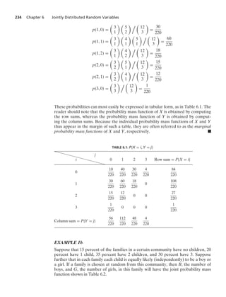
250. Section 6.1 Joint Distribution Functions 235
TABLE 6.2: P{B = i, G = j}
j
i 0 1 2 3 Row sum = P{B = i}
0 .15 .10 .0875 .0375 .3750
1 .10 .175 .1125 0 .3875
2 .0875 .1125 0 0 .2000
3 .0375 0 0 0 .0375
Columnsum = P{G = j} .3750 .3875 .2000 .0375
The probabilities shown in Table 6.2 are obtained as follows:
P{B = 0, G = 0} = P{no children} = .15
P{B = 0, G = 1} = P{1 girl and total of 1 child}
= P{1 child}P{1 girl|1 child} = (.20)
1
2
P{B = 0, G = 2} = P{2 girls and total of 2 children}
= P{2 children}P{2 girls|2 children} = (.35)
1
2
2
We leave the verification of the remaining probabilities in the table to the reader. .
We say that X and Y are jointly continuous if there exists a function f(x, y), defined
for all real x and y, having the property that, for every set C of pairs of real numbers
(that is, C is a set in the two-dimensional plane),
P{(X, Y) ∈ C} =
* *
(x,y)∈C
f(x, y) dx dy (1.3)
The function f(x, y) is called the joint probability density function of X and Y. If A
and B are any sets of real numbers, then, by defining C = {(x, y) : x ∈ A, y ∈ B}, we
see from Equation (1.3) that
P{X ∈ A, Y ∈ B} =
*
B
*
A
f(x, y) dx dy (1.4)
Because
F(a, b) = P{X ∈ (−q, a], Y ∈ (−q, b]}
=
* b
−q
* a
−q
f(x, y) dx dy
it follows, upon differentiation, that
f(a, b) =
∂2
∂a ∂b
F(a, b)
wherever the partial derivatives are defined. Another interpretation of the joint den-
sity function, obtained from Equation (1.4), is

251. 236 Chapter 6 Jointly Distributed Random Variables
P{a X a + da, b Y b + db} =
* d+db
b
* a+da
a
f(x, y) dx dy
L f(a, b) da db
when da and db are small and f(x, y) is continuous at a, b. Hence, f(a, b) is a measure
of how likely it is that the random vector (X, Y) will be near (a, b).
If X and Y are jointly continuous, they are individually continuous, and their prob-
ability density functions can be obtained as follows:
P{X ∈ A} = P{X ∈ A, Y ∈ (−q, q)}
=
*
A
* q
−q
f(x, y) dy dx
=
*
A
fX(x) dx
where
fX(x) =
* q
−q
f(x, y) dy
is thus the probability density function of X. Similarly, the probability density func-
tion of Y is given by
fY(y) =
* q
−q
f(x, y) dx
EXAMPLE 1c
The joint density function of X and Y is given by
f(x, y) =
0
2e−xe−2y 0 x q, 0 y q
0 otherwise
Compute (a) P{X 1, Y 1}, (b) P{X Y}, and (c) P{X a}.
Solution. (a)
P{X 1, Y 1} =
* 1
0
* q
1
2e−x
e−2y
dx dy
=
* 1
0
2e−2y
−e−x
6
6q
1
dy
= e−1
* 1
0
2e−2y
dy
= e−1
(1 − e−2
)
(b)
P{X Y} =
* *
(x,y):xy
2e−x
e−2y
dx dy
=
* q
0
* y
0
2e−x
e−2y
dx dy

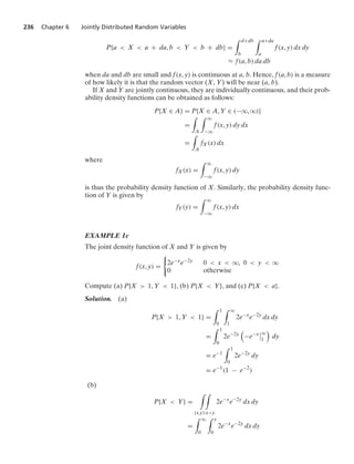
252. Section 6.1 Joint Distribution Functions 237
=
* q
0
2e−2y
(1 − e−y
)dy
=
* q
0
2e−2y
dy −
* q
0
2e−3y
dy
= 1 −
2
3
=
1
3
(c)
P{X a} =
* a
0
* q
0
2e−2y
e−x
dy dx
=
* a
0
e−x
dx
= 1 − e−a
.
EXAMPLE 1d
Consider a circle of radius R, and suppose that a point within the circle is randomly
chosen in such a manner that all regions within the circle of equal area are equally
likely to contain the point. (In other words, the point is uniformly distributed within
the circle.) If we let the center of the circle denote the origin and define X and Y to be
the coordinates of the point chosen (Figure 6.1), then, since (X, Y) is equally likely
to be near each point in the circle, it follows that the joint density function of X and
Y is given by
f(x, y) =
0
c ifx2 + y2 … R2
0 ifx2 + y2 R2
for some value of c.
(a) Determine c.
(b) Find the marginal density functions of X and Y.
(c) Compute the probability that D, the distance from the origin of the point selected,
is less than or equal to a.
(d) Find E [D].
(0, 0)
(X, Y)
R
x
y
FIGURE 6.1: Joint probability distribution.

253. 238 Chapter 6 Jointly Distributed Random Variables
Solution. (a) Because * q
−q
* q
−q
f(x, y) dy dx = 1
it follows that
c
* *
x2+y2…R2
dy dx = 1
We can evaluate
--
x2+y2…R2 dy dx either by using polar coordinates or,
more simply, by noting that it represents the area of the circle and is thus equal
to πR2. Hence,
c =
1
πR2
(b)
fX(x) =
* q
−q
f(x, y) dy
=
1
πR2
*
x2+y2…R2
dy
=
1
πR2
* c
−c
dy, where c =
.
R2 − x2
=
2
πR2
.
R2 − x2 x2
… R2
and it equals 0 when x2 R2. By symmetry, the marginal density of Y is given by
fY(y) =
2
πR2
8
R2 − y2 y2
… R2
= 0 y2
R2
(c) The distribution function of D =
.
X2 + Y2, the distance from the origin, is
obtained as follows: For 0 … a … R,
FD(a) = P{
.
X2 + Y2 … a}
= P{X2
+ Y2
… a2
}
=
**
x2+y2…a2
f(x, y) dy dx
=
1
πR2
**
x2+y2…a2
dy dx
=
πa2
πR2
=
a2
R2
where we have used the fact that
--
x2+y2…a2 dy dx is the area of a circle of radius
a and thus is equal to πa2.

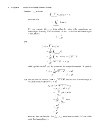
254. Section 6.1 Joint Distribution Functions 239
(d) From part (c), the density function of D is
fD(a) =
2a
R2
0 … a … R
Hence,
E[D] =
2
R2
* R
0
a2
da =
2R
3 .
EXAMPLE 1e
The joint density of X and Y is given by
f(x, y) =
%
e−(x+y) 0 x q, 0 y q
0 otherwise
Find the density function of the random variable X/Y.
Solution. We start by computing the distribution function of X/Y. For a 0,
FX/Y(a) = P
%
X
Y
… a
/
=
* *
x/y…a
e−(x+y)
dx dy
=
* q
0
* ay
0
e−(x+y)
dx dy
=
* q
0
(1 − e−ay
)e−y
dy
=
0
−e−y
+
e−(a+1)y
a + 1
76
6
6
6
6
6
q
0
= 1 −
1
a + 1
Differentiation shows that the density function of X/Y is given by fX/Y(a) = 1/
(a + 1)2, 0 a q. .
We can also define joint probability distributions for n random variables in exactly
the same manner as we did for n = 2. For instance, the joint cumulative probabil-
ity distribution function F(a1, a2, ... , an) of the n random variables X1, X2, ... , Xn is
defined by
F(a1, a2, ... , an) = P{X1 … a1, X2 … a2, ... , Xn … an}
Further, the n random variables are said to be jointly continuous if there exists a
function f(x1, x2, ... , xn), called the joint probability density function, such that, for
any set C in n-space,
P{(X1, X2, ... , Xn) ∈ C} =
**
· · ·
*
(x1,...,xn)∈C
f(x1, ... , xn)dx1dx2 · · · dxn

255. 240 Chapter 6 Jointly Distributed Random Variables
In particular, for any n sets of real numbers A1, A2, ... , An,
P{X1 ∈ A1, X2, ∈ A2, ... , Xn ∈ An}
=
*
An
*
An−1
· · ·
*
A1
f(x1, ... , xn) dx1dx2 · · · dxn
EXAMPLE 1f The multinomial distribution
One of the most important joint distributions is the multinomial distribution, which
arises when a sequence of n independent and identical experiments is performed.
Suppose that each experiment can result in any one of r possible outcomes, with
respective probabilities p1, p2, ... , pr,
r
i=1
pi = 1. If we let Xi denote the number of the
n experiments that result in outcome number i, then
P{X1 = n1, X2 = n2, ... , Xr = nr} =
n!
n1!n2! · · · nr!
p
n1
1 p
n2
2 · · · pnr
r (1.5)
whenever
r
i=1
ni = n.
Equation (1.5) is verified by noting that any sequence of outcomes for the n experi-
ments that leads to outcome i occurring ni times for i = 1, 2, ... , r will, by the assumed
independence of experiments, have probability p
n1
1 p
n2
2 ... pnr
r of occurring. Because
there are n!/(n1!n2! ... nr!) such sequences of outcomes (there are n!/n1! ... nr! dif-
ferent permutations of n things of which n1 are alike, n2 are alike, ... , nr are alike),
Equation (1.5) is established. The joint distribution whose joint probability mass func-
tion is specified by Equation (1.5) is called the multinomial distribution. Note that
when r = 2, the multinomial reduces to the binomial distribution.
Note also that any sum of a fixed set of the X
i s will have a binomial distribution.
That is, if N ( {1, 2, ... , r}, then i∈N Xi will be a binomial random variable with
parameters n and p = i∈N pi. This follows because i∈N Xi represents the number
of the n experiments whose outcome is in N, and each experiment will independently
have such an outcome with probability i∈N pi.
As an application of the multinomial distribution, suppose that a fair die is rolled
9 times. The probability that 1 appears three times, 2 and 3 twice each, 4 and 5 once
each, and 6 not at all is
9!
3!2!2!1!1!0!
1
6
3
1
6
2
1
6
2
1
6
1
1
6
1
1
6
0
=
9!
3!2!2!
1
6
9
.
6.2 INDEPENDENT RANDOM VARIABLES
The random variables X and Y are said to be independent if, for any two sets of real
numbers A and B,
P{X ∈ A, Y ∈ B} = P{X ∈ A}P{Y ∈ B} (2.1)
In other words, X and Y are independent if, for all A and B, the events EA = {X ∈ A}
and FB = {Y ∈ B} are independent.
It can be shown by using the three axioms of probability that Equation (2.1) will
follow if and only if, for all a, b,
P{X … a, Y … b} = P{X … a}P{Y … b}

256. Section 6.2 Independent Random Variables 241
Hence, in terms of the joint distribution function F of X and Y, X and Y are inde-
pendent if
F(a, b) = FX(a)FY(b) for all a, b
When X and Y are discrete random variables, the condition of independence (2.1) is
equivalent to
p(x, y) = pX(x)pY(y) for all x, y (2.2)
The equivalence follows because, if Equation (2.1) is satisfied, then we obtain Equa-
tion (2.2) by letting A and B be, respectively, the one-point sets A = {x} and B = {y}.
Furthermore, if Equation (2.2) is valid, then, for any sets A, B,
P{X ∈ A, Y ∈ B} =
y∈B
x∈A
p(x, y)
=
y∈B
x∈A
pX(x)pY(y)
=
y∈B
pY(y)
x∈A
pX(x)
= P{Y ∈ B}P{X ∈ A}
and Equation (2.1) is established.
In the jointly continuous case, the condition of independence is equivalent to
f(x, y) = fX(x)fY(y) for all x, y
Thus, loosely speaking, X and Y are independent if knowing the value of one does
not change the distribution of the other. Random variables that are not independent
are said to be dependent.
EXAMPLE 2a
Suppose that n + m independent trials having a common probability of success p are
performed. If X is the number of successes in the first n trials, and Y is the number
of successes in the final m trials, then X and Y are independent, since knowing the
number of successes in the first n trials does not affect the distribution of the number
of successes in the final m trials (by the assumption of independent trials). In fact, for
integral x and y,
P{X = x, Y = y} =
n
x
px
(1 − p)n−x
m
y
py
(1 − p)m−y 0 … x … n,
0 … y … m
= P{X = x}P{Y = y}
In contrast, X and Z will be dependent, where Z is the total number of successes in
the n + m trials. (Why?) .
EXAMPLE 2b
Suppose that the number of people who enter a post office on a given day is a Poisson
random variable with parameter λ. Show that if each person who enters the post office
is a male with probability p and a female with probability 1 − p, then the number of
males and females entering the post office are independent Poisson random variables
with respective parameters λp and λ(1 − p).

257. 242 Chapter 6 Jointly Distributed Random Variables
Solution. Let X and Y denote, respectively, the number of males and females that
enter the post office. We shall show the independence of X and Y by establishing
Equation (2.2). To obtain an expression for P{X = i, Y = j}, we condition on X + Y
as follows:
P{X = i, Y = j} = P{X = i, Y = j|X + Y = i + j}P{X + Y = i + j}
+ P{X = i, Y = j|X + Y Z i + j}P{X + Y Z i + j}
[Note that this equation is merely a special case of the formula P(E) = P(E|F)P(F) +
P(E|Fc)P(Fc).]
Since P{X = i, Y = j|X + Y Z i + j} is clearly 0, we obtain
P{X = i, Y = j} = P{X = i, Y = j|X + Y = i + j}P{X + Y = i + j} (2.3)
Now, because X + Y is the total number of people who enter the post office, it
follows, by assumption, that
P{X + Y = i + j} = e−λ λi+j
(i + j)!
(2.4)
Furthermore, given that i + j people do enter the post office, since each person
entering will be male with probability p, it follows that the probability that exactly
i of them will be male (and thus j of them female) is just the binomial probability
i + j
i
pi(1 − p)j. That is,
P{X = i, Y = j|X + Y = i + j} =
i + j
i
pi
(1 − p)j
(2.5)
Substituting Equations (2.4) and (2.5) into Equation (2.3) yields
P{X = i, Y = j} =
i + j
i
pi
(1 − p)j
e−λ λi+j
(i + j)!
= e−λ (λp)i
i!j!
[λ(1 − p)]j
=
e−λp(λp)i
i!
e−λ(1−p) [λ(1 − p)]j
j!
(2.6)
Hence,
P{X = i} = e−λp (λp)i
i!
j
e−λ(1−p) [λ(1 − p)]j
j!
= e−λp (λp)i
i!
(2.7)
and similarly,
P{Y = j} = e−λ(1−p) [λ(1 − p)]j
j!
(2.8)
Equations (2.6), (2.7), and (2.8) establish the desired result. .

258. Section 6.2 Independent Random Variables 243
EXAMPLE 2c
A man and a woman decide to meet at a certain location. If each of them indepen-
dently arrives at a time uniformly distributed between 12 noon and 1 P.M., find the
probability that the first to arrive has to wait longer than 10 minutes.
Solution. If we let X and Y denote, respectively, the time past 12 that the man and
the woman arrive, then X and Y are independent random variables, each of which is
uniformly distributed over (0, 60). The desired probability, P{X + 10 Y} + P{Y +
10 X}, which, by symmetry, equals 2P{X + 10 Y}, is obtained as follows:
2P{X + 10 Y} = 2
* *
x+10y
f(x, y) dx dy
= 2
* *
x+10y
fX(x)fY(y) dx dy
= 2
* 60
10
* y−10
0
1
60
2
dx dy
=
2
(60)2
* 60
10
(y − 10) dy
=
25
36 .
Our next example presents the oldest problem dealing with geometrical probabil-
ities. It was first considered and solved by Buffon, a French naturalist of the 18th
century, and is usually referred to as Buffon’s needle problem.
EXAMPLE 2d Buffon’s needle problem
A table is ruled with equidistant parallel lines a distance D apart. A needle of length L,
where L … D, is randomly thrown on the table. What is the probability that the nee-
dle will intersect one of the lines (the other possibility being that the needle will be
completely contained in the strip between two lines)?
Solution. Let us determine the position of the needle by specifying (1) the distance X
from the middle point of the needle to the nearest parallel line and (2) the angle θ
between the needle and the projected line of length X. (See Figure 6.2.) The needle
will intersect a line if the hypotenuse of the right triangle in Figure 6.2 is less than
L/2—that is, if
X
cos θ
L
2
or X
L
2
cos θ
␪
X
FIGURE 6.2

259. 244 Chapter 6 Jointly Distributed Random Variables
As X varies between 0 and D/2 and θ between 0 and π/2, it is reasonable to assume
that they are independent, uniformly distributed random variables over these respec-
tive ranges. Hence,
P
%
X
L
2
cos θ
/
=
* *
xL/2 cos y
fX(x)fθ (y) dx dy
=
4
πD
* π/2
0
* L/2 cos y
0
dx dy
=
4
πD
* π/2
0
L
2
cos y dy
=
2L
πD .
∗EXAMPLE 2e Characterization of the normal distribution
Let X and Y denote the horizontal and vertical miss distances when a bullet is fired
at a target, and assume that
1. X and Y are independent continuous random variables having differentiable
density functions.
2. The joint density f(x, y) = fX(x)fY(y) of X and Y depends on (x, y) only through
x2 + y2.
Loosely put, assumption 2 states that the probability of the bullet landing on any
point of the x–y plane depends only on the distance of the point from the target and
not on its angle of orientation. An equivalent way of phrasing this assumption is to
say that the joint density function is rotation invariant.
It is a rather interesting fact that assumptions 1 and 2 imply that X and Y are
normally distributed random variables. To prove this, note first that the assumptions
yield the relation
f(x, y) = fX(x)fY(y) = g(x2
+ y2
) (2.9)
for some function g. Differentiating Equation (2.9) with respect to x yields
f
X(x)fY(y) = 2xg
(x2
+ y2
) (2.10)
Dividing Equation (2.10) by Equation (2.9) gives
f
X(x)
fX(x)
=
2xg(x2 + y2)
g(x2 + y2)
or
f
X(x)
2xfX(x)
=
g(x2 + y2)
g(x2 + y2)
(2.11)
Because the value of the left-hand side of Equation (2.11) depends only on x,
whereas the value of the right-hand side depends on x2 + y2, it follows that the
left-hand side must be the same for all x. To see this, consider any x1, x2 and let y1, y2
be such that x2
1 + y2
1 = x2
2 + y2
2. Then, from Equation (2.11), we obtain
f
X(x1)
2x1fX(x1)
=
g(x2
1 + y2
1)
g(x2
1 + y2
1)
=
g(x2
2 + y2
2)
g(x2
2 + y2
2)
=
f
X(x2)
2x2fX(x2)

260. Section 6.2 Independent Random Variables 245
Hence,
f
X(x)
xfX(x)
= c or
d
dx
(log fX(x)) = cx
which implies, upon integration of both sides, that
log fX(x) = a +
cx2
2
or fX(x) = kecx2/2
Since
- q
−q fX(x) dx = 1, it follows that c is necessarily negative, and we may write
c = −1/σ2. Thus,
fX(x) = ke−x2/2σ2
That is, X is a normal random variable with parameters μ = 0 and σ2. A similar
argument can be applied to fY(y) to show that
fY(y) =
1
√
2π σ
e−y2/2σ2
Furthermore, it follows from assumption 2 that σ2 = σ2 and that X and Y are thus
independent, identically distributed normal random variables with parameters μ = 0
and σ2. .
A necessary and sufficient condition for the random variables X and Y to be
independent is for their joint probability density function (or joint probability mass
function in the discrete case) f(x, y) to factor into two terms, one depending only on
x and the other depending only on y.
Proposition 2.1. The continuous (discrete) random variables X and Y are indepen-
dent if and only if their joint probability density (mass) function can be expressed as
fX,Y(x, y) = h(x)g(y) − q x q, −q y q
Proof. Let us give the proof in the continuous case. First, note that independence
implies that the joint density is the product of the marginal densities of X and Y, so
the preceding factorization will hold when the random variables are independent.
Now, suppose that
fX,Y(x, y) = h(x)g(y)
Then
1 =
* q
−q
* q
−q
fX,Y(x, y) dx dy
=
* q
−q
h(x) dx
* q
−q
g(y) dy
= C1C2
where C1 =
- q
−q h(x) dx and C2 =
- q
−q g(y) dy. Also,
fX(x) =
* q
−q
fX,Y(x, y) dy = C2h(x)
fY(y) =
* q
−q
fX,Y(x, y) dx = C1g(y)

261. 246 Chapter 6 Jointly Distributed Random Variables
Since C1C2 = 1, it follows that
fX,Y(x, y) = fX(x)fY(y)
and the proof is complete.
EXAMPLE 2f
If the joint density function of X and Y is
f(x, y) = 6e−2x
e−3y
0 x q, 0 y q
and is equal to 0 outside this region, are the random variables independent? What if
the joint density function is
f(x, y) = 24xy 0 x 1, 0 y 1, 0 x + y 1
and is equal to 0 otherwise?
Solution. In the first instance, the joint density function factors, and thus the random
variables, are independent (with one being exponential with rate 2 and the other
exponential with rate 3). In the second instance, because the region in which the joint
density is nonzero cannot be expressed in the form x ∈ A, y ∈ B, the joint density does
not factor, so the random variables are not independent. This can be seen clearly by
letting
I(x, y) =
%
1 if 0 x 1, 0 y 1, 0 x + y 1
0 otherwise
and writing
f(x, y) = 24xy I(x, y)
which clearly does not factor into a part depending only on x and another depending
only on y. .
The concept of independence may, of course, be defined for more than two random
variables. In general, the n random variables X1, X2, ... , Xn are said to be indepen-
dent if, for all sets of real numbers A1, A2, ... , An,
P{X1 ∈ A1, X2 ∈ A2, ... , Xn ∈ An} =
n
i=1
P{Xi ∈ Ai}
As before, it can be shown that this condition is equivalent to
P{X1 … a1, X2 … a2, ... , Xn … an}
=
n
i=1
P{Xi … ai} for all a1, a2, ... , an
Finally, we say that an infinite collection of random variables is independent if every
finite subcollection of them is independent.
EXAMPLE 2g How can a computer choose a random subset?
Most computers are able to generate the value of, or simulate, a uniform (0, 1) random
variable by means of a built-in subroutine that (to a high degree of approximation)

262. Section 6.2 Independent Random Variables 247
produces such “random numbers.” As a result, it is quite easy for a computer to sim-
ulate an indicator (that is, a Bernoulli) random variable. Suppose I is an indicator
variable such that
P{I = 1} = p = 1 − P{I = 0}
The computer can simulate I by choosing a uniform (0, 1) random number U and
then letting
I =
1 if U p
0 if U Ú p
Suppose that we are interested in having the computer select k, k … n, of the num-
bers 1, 2, ... , n in such a way that each of the
n
k
subsets of size k is equally likely
to be chosen. We now present a method that will enable the computer to solve this
task. To generate such a subset, we will first simulate, in sequence, n indicator vari-
ables I1, I2, ... , In, of which exactly k will equal 1. Those i for which Ii = 1 will then
constitute the desired subset.
To generate the random variables I1, ... , In, start by simulating n independent uni-
form (0, 1) random variables U1, U2, ... , Un. Now define
I1 =
⎧
⎪
⎨
⎪
⎩
1 if U1
k
n
0 otherwise
and then, once I1, ... , Ii are determined, recursively set
Ii+1 =
⎧
⎪
⎨
⎪
⎩
1 if Ui+1
k − (I1 + · · · + Ii)
n − i
0 otherwise
In words, at the (i + 1)th stage we set Ii+1 equal to 1 (and thus put i + 1 into the
desired subset) with a probability equal to the remaining number of places in the sub-
set
⎛
⎝namely, k −
i
j=1
Ij
⎞
⎠, divided by the remaining number of possibilities (namely,
n − i). Hence, the joint distribution of I1, I2, ... , In is determined from
P{I1 = 1} =
k
n
P{Ii+1 = 1|I1, ... , Ii} =
k −
i
j=1
Ij
n − i
1 i n
The proof that the preceding formula results in all subsets of size k being equally
likely to be chosen is by induction on k + n. It is immediate when k + n = 2 (that
is, when k = 1, n = 1), so assume it to be true whenever k + n … l. Now, suppose
that k + n = l + 1, and consider any subset of size k—say, i1 … i2 … · · · … ik—and
consider the following two cases.

263. 248 Chapter 6 Jointly Distributed Random Variables
Case 1: i1 = 1
P{I1 = Ii2 = · · · = Iik
= 1, Ij = 0 otherwise}
= P{I1 = 1}P{Ii2 = · · · = Iik
= 1, Ij = 0 otherwise|I1 = 1}
Now given that I1 = 1, the remaining elements of the subset are chosen as if a
subset of size k − 1 were to be chosen from the n − 1 elements 2, 3, ... , n. Hence,
by the induction hypothesis, the conditional probability that this will result in a given
subset of size k − 1 being selected is 1/
n − 1
k − 1
. Hence,
P{I1 = Ii2 = · · · = Iik
= 1, Ij = 0 otherwise}
=
k
n
1
n − 1
k − 1
=
1
n
k
Case 2: i1 Z 1
P{Ii1
= Ii2 = · · · = Iik
= 1, Ij = 0 otherwise}
= P{Ii1
= · · · = Iik
= 1, Ij = 0 otherwise|I1 = 0}P{I1 = 0}
=
1
n − 1
k
1 −
k
n
=
1
n
k
where the induction hypothesis was used to evaluate the preceding conditional prob-
ability.
Thus, in all cases, the probability that a given subset of size k will be the subset
chosen is 1
n
k
. .
Remark. The foregoing method for generating a random subset has a very low
memory requirement. A faster algorithm that requires somewhat more memory is
presented in Section 10.1. (The latter algorithm uses the last k elements of a random
permutation of 1, 2, ... , n.) .
EXAMPLE 2h
Let X, Y, Z be independent and uniformly distributed over (0, 1). Compute P{X Ú
YZ}.
Solution. Since
fX,Y,Z(x, y, z) = fX(x)fY(y)fZ(z) = 1 0 … x … 1, 0 … y … 1, 0 … z … 1
we have
P{X Ú YZ} =
* * *
xÚyz
fX, Y, Z(x, y, z) dx dy dz
=
* 1
0
* 1
0
* 1
yz
dx dy dz

264. Section 6.2 Independent Random Variables 249
=
* 1
0
* 1
0
(1 − yz) dy dz
=
* 1
0
1 −
z
2
dz
=
3
4 .
EXAMPLE 2i Probabilistic interpretation of half-life
Let N(t) denote the number of nuclei contained in a radioactive mass of material at
time t. The concept of half-life is often defined in a deterministic fashion by stating
this it is an empirical fact that, for some value h, called the half-life,
N(t) = 2−t/h
N(0) t 0
[Note that N(h) = N(0)/2.] Since the preceding implies that, for any nonnegative s
and t,
N(t + s) = 2−(s+t)/h
N(0) = 2−t/h
N(s)
it follows that no matter how much time s has already elapsed, in an additional time t
the number of existing nuclei will decrease by the factor 2−t/h.
Because the deterministic relationship just given results from observations of radio-
active masses containing huge numbers of nuclei, it would seem that it might be
consistent with a probabilistic interpretation. The clue to deriving the appropriate
probability model for half-life resides in the empirical observation that the propor-
tion of decay in any time interval depends neither on the total number of nuclei at
the beginning at the interval nor on the location of this interval (since N(t + s)/N(s)
depends neither on N(s) nor on s). Thus, it appears that the individual nuclei act inde-
pendently and with a memoryless life distribution. Consequently, since the unique life
distribution that is memoryless is the exponential distribution, and since exactly one-
half of a given amount of mass decays every h time units, we propose the following
probabilistic model for radioactive decay.
Probabilistic interpretation of the half-life h: The lifetimes of the individual nuclei
are independent random variables having a life distribution that is exponential with
median equal to h. That is, if L represents the lifetime of a given nucleus, then
P{L t} = 1 − 2−t/h
(Because P{L h} = 1
2 and the preceding can be written as
P{L t} = 1 − exp
%
−t
log 2
h
/
it can be seen that L indeed has an exponential distribution with median h.)
Note that, under the probabilistic interpretation of half-life just given, if one starts
with N(0) nuclei at time 0, then N(t), the number of nuclei that remain at time t,
will have a binomial distribution with parameters n = N(0) and p = 2−t/h. Results of
Chapter 8 will show that this interpretation of half-life is consistent with the determin-
istic model when considering the proportion of a large number of nuclei that decay
over a given time frame. However, the difference between the deterministic and prob-
abilistic interpretation becomes apparent when one considers the actual number of

265. 250 Chapter 6 Jointly Distributed Random Variables
decayed nuclei. We will now indicate this with regard to the question of whether
protons decay.
There is some controversy over whether or not protons decay. Indeed, one theory
predicts that protons should decay with a half-life of about h = 1030 years. To check
this prediction empirically, it has been suggested that one follow a large number of
protons for, say, one or two years and determine whether any of them decay within
that period. (Clearly, it would not be feasible to follow a mass of protons for 1030
years to see whether one-half of it decays.) Let us suppose that we are able to keep
track of N(0) = 1030 protons for c years. The number of decays predicted by the
deterministic model would then be given by
N(0) − N(c) = h(1 − 2−c/h
)
=
1 − 2−c/h
1/h
L lim
x→0
1 − 2−cx
x
since
1
h
= 10−30
L 0
= lim
x→0
(c2−cx
log 2) by L’Hôpital’s rule
= c log 2 L .6931c
For instance, the deterministic model predicts that in 2 years there should be 1.3863
decays, and it would thus appear to be a serious blow to the hypothesis that protons
decay with a half-life of 1030 years if no decays are observed over those 2 years.
Let us now contrast the conclusions just drawn with those obtained from the prob-
abilistic model. Again, let us consider the hypothesis that the half-life of protons is
h = 1030 years, and suppose that we follow h protons for c years. Since there is a
huge number of independent protons, each of which will have a very small probabil-
ity of decaying within this time period, it follows that the number of protons which
decay will have (to a very strong approximation) a Poisson distribution with parame-
ter equal to h(1 − 2−c/h) L c log 2. Thus,
P{0 decays} = e−c log 2
= e− log(2c)
=
1
2c
and, in general,
P{n decays} =
2−c[c log 2]n
n!
n Ú 0
Thus we see that even though the average number of decays over 2 years is (as pre-
dicted by the deterministic model) 1.3863, there is 1 chance in 4 that there will not
be any decays, thereby indicating that such a result in no way invalidates the original
hypothesis of proton decay. .
Remark. Independence is a symmetric relation. The random variables X and Y
are independent if their joint density function (or mass function in the discrete case)
is the product of their individual density (or mass) functions. Therefore, to say that
X is independent of Y is equivalent to saying that Y is independent of X—or just
that X and Y are independent. As a result, in considering whether X is independent
of Y in situations where it is not at all intuitive that knowing the value of Y will not
change the probabilities concerning X, it can be beneficial to interchange the roles of

266. Section 6.2 Independent Random Variables 251
X and Y and ask instead whether Y is independent of X. The next example illustrates
this point. .
EXAMPLE 2j
If the initial throw of the dice in the game of craps results in the sum of the dice
equaling 4, then the player will continue to throw the dice until the sum is either 4 or
7. If this sum is 4, then the player wins, and if it is 7, then the player loses. Let N denote
the number of throws needed until either 4 or 7 appears, and let X denote the value
(either 4 or 7) of the final throw. Is N independent of X? That is, does knowing which
of 4 or 7 occurs first affect the distribution of the number of throws needed until that
number appears? Most people do not find the answer to this question to be intuitively
obvious. However, suppose that we turn it around and ask whether X is independent
of N. That is, does knowing how many throws it takes to obtain a sum of either 4 or
7 affect the probability that that sum is equal to 4? For instance, suppose we know
that it takes n throws of the dice to obtain a sum of either 4 or 7. Does this affect the
probability distribution of the final sum? Clearly not, since all that is important is that
its value is either 4 or 7, and the fact that none of the first n − 1 throws were either 4
or 7 does not change the probabilities for the nth throw. Thus, we can conclude that
X is independent of N, or equivalently, that N is independent of X.
As another example, let X1, X2, ... be a sequence of independent and identically
distributed continuous random variables, and suppose that we observe these random
variables in sequence. If Xn Xi for each i = 1, ... , n − 1, then we say that Xn is
a record value. That is, each random variable that is larger than all those preceding
it is called a record value. Let An denote the event that Xn is a record value. Is An+1
independent of An? That is, does knowing that the nth random variable is the largest
of the first n change the probability that the (n + 1)st random variable is the largest
of the first n + 1? While it is true that An+1 is independent of An, this may not be
intuitively obvious. However, if we turn the question around and ask whether An is
independent of An+1, then the result is more easily understood. For knowing that
the (n + 1)st value is larger than X1, ... , Xn clearly gives us no information about
the relative size of Xn among the first n random variables. Indeed, by symmetry, it is
clear that each of these n random variables is equally likely to be the largest of this
set, so P(An|An+1) = P(An) = 1/n. Hence, we can conclude that An and An+1 are
independent events. .
Remark. It follows from the identity
P{X1 … a1, ... , Xn … an}
= P{X1 … a1}P{X2 … a2|X1 … a1} · · · P{Xn … an|X1 … a1, ... , Xn−1 … an−1}
that the independence of X1, ... , Xn can be established sequentially. That is, we can
show that these random variables are independent by showing that
X2 is independent of X1
X3 is independent of X1, X2
X4 is independent of X1, X2, X3
#
#
#
Xn is independent of X1, ... , Xn−1

267. 252 Chapter 6 Jointly Distributed Random Variables
6.3 SUMS OF INDEPENDENT RANDOM VARIABLES
It is often important to be able to calculate the distribution of X + Y from the dis-
tributions of X and Y when X and Y are independent. Suppose that X and Y are
independent, continuous random variables having probability density functions fX
and fY. The cumulative distribution function of X + Y is obtained as follows:
FX+Y(a) = P{X + Y … a}
=
* *
x+y…a
fX(x)fY(y) dx dy
=
* q
−q
* a−y
−q
fX(x)fY(y) dx dy (3.1)
=
* q
−q
* a−y
−q
fX(x) dxfY(y) dy
=
* q
−q
FX(a − y)fY(y) dy
The cumulative distribution function FX+Y is called the convolution of the distribu-
tions FX and FY (the cumulative distribution functions of X and Y, respectively).
By differentiating Equation (3.1), we find that the probability density function
fX+Y of X + Y is given by
fX+Y(a) =
d
da
* q
−q
FX(a − y)fY(y) dy
=
* q
−q
d
da
FX(a − y)fY(y) dy (3.2)
=
* q
−q
fX(a − y)fY(y) dy
6.3.1 Identically Distributed Uniform Random Variables
It is not difficult to determine the density function of the sum of two independent
uniform (0, 1) random variables.
EXAMPLE 3a Sum of two independent uniform random variables
If X and Y are independent random variables, both uniformly distributed on (0, 1),
calculate the probability density of X + Y.
Solution. From Equation (3.2), since
fX(a) = fY(a) =
%
1 0 a 1
0 otherwise
we obtain
fX+Y(a) =
* 1
0
fX(a − y) dy
For 0 … a … 1, this yields
fX+Y(a) =
* a
0
dy = a

268. Section 6.3 Sums of Independent Random Variables 253
1
1 2
x
f(x)
0
FIGURE 6.3: Triangular density function.
For 1 a 2, we get
fX+Y(a) =
* 1
a−1
dy = 2 − a
Hence,
fX+Y(a) =
⎧
⎨
⎩
a 0 … a … 1
2 − a 1 a 2
0 otherwise
Because of the shape of its density function (see Figure 6.3), the random variable
X + Y is said to have a triangular distribution. .
Now, suppose that X1, X2, ... , Xn are independent uniform (0, 1) random variables,
and let
Fn(x) = P{X1 + ... + Xn … x}
Whereas a general formula for Fn(x) is messy, it has a particularly nice form when
x … 1. Indeed, we now use mathematical induction to prove that
Fn(x) = xn
/n! , 0 … x … 1
Because the proceeding equation is true for n = 1, assume that
Fn−1(x) = xn−1
/(n − 1)! , 0 … x … 1
Now, writing
n
i=1
Xi =
n−1
i=1
Xi + Xn
and using the fact that the Xi are all nonnegative, we see from Equation 3.1 that, for
0 … x … 1,
Fn(x) =
* 1
0
Fn−1(x − y)fXn (y)dy
=
1
(n − 1)!
* x
0
(x − y)n−1
dy by the induction hypothesis
= xn
/n!
which completes the proof.

269. 254 Chapter 6 Jointly Distributed Random Variables
For an interesting application of the preceding formula, let us use it to determine
the expected number of independent uniform (0, 1) random variables that need to
be summed to exceed 1. That is, with X1, X2, ... being independent uniform (0, 1)
random variables, we want to determine E[N], where
N = min{n : X1 + ... + Xn 1}
Noting that N is greater than n 0 if and only if X1 + ... + Xn … 1, we see that
P{N n} = Fn(1) = 1/n! , n 0
Because
P{N 0} = 1 = 1/0!
we see that, for n 0,
P{N = n} = P{N n − 1} − P{N n} =
1
(n − 1)!
−
1
n!
=
n − 1
n!
Therefore,
E[N] =
q
n=1
n(n − 1)
n!
=
q
n=2
1
(n − 2)!
= e
That is, the mean number of independent uniform (0, 1) random variables that must
be summed for the sum to exceed 1 is equal to e.
6.3.2 Gamma Random Variables
Recall that a gamma random variable has a density of the form
f(y) =
λe−λy(λy)t−1
(t)
0 y q
An important property of this family of distributions is that, for a fixed value of λ, it
is closed under convolutions.
Proposition 3.1. If X and Y are independent gamma random variables with respec-
tive parameters (s, λ) and (t, λ), then X + Y is a gamma random variable with param-
eters (s + t, λ).
Proof. Using Equation (3.2), we obtain
fX+Y(a) =
1
(s)(t)
* a
0
λe−λ(a−y)
[λ(a − y)]s−1
λe−λy
(λy)t−1
dy
= Ke−λa
* a
0
(a − y)s−1
yt−1
dy
= Ke−λa
as+t−1
* 1
0
(1 − x)s−1
xt−1
dx by letting x =
y
a
= Ce−λa
as+t−1

270. Section 6.3 Sums of Independent Random Variables 255
where C is a constant that does not depend on a. But, as the preceding is a density
function and thus must integrate to 1, the value of C is determined, and we have
fX+Y(a) =
λe−λa(λa)s+t−1
(s + t)
Hence, the result is proved.
It is now a simple matter to establish, by using Proposition 3.1 and induction, that if
Xi, i = 1, ... , n are independent gamma random variables with respective parameters
(ti, λ), i = 1, ... , n, then
n
i=1
Xi is gamma with parameters
n
i=1
ti, λ
. We leave the
proof of this statement as an exercise.
EXAMPLE 3b
Let X1, X2, ... , Xn be n independent exponential random variables, each having param-
eter λ. Then, since an exponential random variable with parameter λ is the same as
a gamma random variable with parameters (1, λ), it follows from Proposition 3.1 that
X1 + X2 + · · · + Xn is a gamma random variable with parameters (n, λ). .
If Z1, Z2, ... , Zn are independent standard normal random variables, then Y K
n
i=1
Z2
i is said to have the chi-squared (sometimes seen as χ2) distribution with n
degrees of freedom. Let us compute the density function of Y. When n = 1, Y = Z2
1,
and from Example 7b of Chapter 5, we see that its probability density function is
given by
fZ2 (y) =
1
2
√
y
[fZ(
√
y) + fZ(−
√
y)]
=
1
2
√
y
2
√
2π
e−y/2
=
1
2e−y/2(y/2)1/2−1
√
π
But we recognize the preceding as the gamma distribution with parameters
1
2 , 1
2
.
[A by-product of this analysis is that
1
2
=
√
π.] But since each Z2
i is gamma
1
2 , 1
2
, it follows from Proposition 3.1 that the χ2 distribution with n degrees of
freedom is just the gamma distribution with parameters
n/2, 1
2
and hence has a
probability density function given by
fχ2 (y) =
1
2
e−y/2
y
2
n/2−1
n
2
y 0
=
e−y/2yn/2−1
2n/2
n
2
y 0

271. 256 Chapter 6 Jointly Distributed Random Variables
When n is an even integer, (n/2) = [(n/2) − 1]!, whereas when n is odd, (n/2) can
be obtained from iterating the relationship (t) = (t − 1)(t − 1) and then using
the previously obtained result that
1
2
=
√
π. [For instance,
5
2
= 3
2
3
2
=
3
2
1
2
1
2
= 3
4
√
π.]
In practice, the chi-squared distribution often arises as the distribution of the square
of the error involved when one attempts to hit a target in n-dimensional space when
the coordinate errors are taken to be independent standard normal random variables.
It is also important in statistical analysis.
6.3.3 Normal Random Variables
We can also use Equation (3.2) to prove the following important result about normal
random variables.
Proposition 3.2. If Xi, i = 1, ... , n, are independent random variables that are nor-
mally distributed with respective parameters μi, σ2
i , i = 1, ... , n, then
n
i=1
Xi is normally
distributed with parameters
n
i=1
μi and
n
i=1
σ2
i .
Proof of Proposition 3.2: To begin, let X and Y be independent normal random
variables with X having mean 0 and variance σ2 and Y having mean 0 and vari-
ance 1. We will determine the density function of X + Y by utilizing Equation (3.2).
Now, with
c =
1
2σ2
+
1
2
=
1 + σ2
2σ2
we have
fX(a − y)fY(y) =
1
√
2πσ
exp
0
−
(a − y)2
2σ2
7
1
√
2π
exp
0
−
y2
2
7
=
1
2πσ
exp
0
−
a2
2σ2
7
exp
0
−c
y2
− 2y
a
1 + σ2
7
Hence, from Equation (3.2),
fX+Y(a) =
1
2πσ
exp
0
−
a2
2σ2
7
exp
0
a2
2σ2(1 + σ2)
7
*
* q
−q
exp
0
−c
y −
a
1 + σ2
2
7
dy
=
1
2πσ
exp
0
−
a2
2(1 + σ2)
7 * q
−q
exp{−cx2
} dx
= C exp
0
−
a2
2(1 + σ2)
7
where C does not depend on a. But this implies that X + Y is normal with mean 0
and variance 1 + σ2.

272. Section 6.3 Sums of Independent Random Variables 257
Now, suppose that X1 and X2 are independent normal random variables with Xi
having mean μi and variance σ2
i , i = 1, 2. Then
X1 + X2 = σ2
X1 − μ1
σ2
+
X2 − μ2
σ2
+ μ1 + μ2
But since (X1 − μ1)/σ2 is normal with mean 0 and variance σ2
1 /σ2
2 , and (X2 − μ2)/σ2
is normal with mean 0 and variance 1, it follows from our previous result that (X1 −
μ1)/σ2 + (X2 − μ2)/σ2 is normal with mean 0 and variance 1 + σ2
1 /σ2
2 , implying
that X1 + X2 is normal with mean μ1 + μ2 and variance σ2
2 (1 + σ2
1 /σ2
2 ) = σ2
1 + σ2
2 .
Thus, Proposition 3.2 is established when n = 2. The general case now follows by
induction. That is, assume that Proposition 3.2 is true when there are n − 1 random
variables. Now consider the case of n, and write
n
i=1
Xi =
n−1
i=1
Xi + Xn
By the induction hypothesis,
n−1
i=1
Xi is normal with mean
n−1
i=1
μi and variance
n−1
i=1
σ2
i .
Therefore, by the result for n = 2,
n
i=1
Xi is normal with mean
n
i=1
μi and variance
n
i=1
σ2
i .
EXAMPLE 3c
A basketball team will play a 44-game season. Twenty-six of these games are against
class A teams and 18 are against class B teams. Suppose that the team will win each
game against a class A team with probability .4 and will win each game against a class
B team with probability .7. Suppose also that the results of the different games are
independent. Approximate the probability that
(a) the team wins 25 games or more;
(b) the team wins more games against class A teams than it does against class B
teams.
Solution. (a) Let XA and XB respectively denote the number of games the team
wins against class A and against class B teams. Note that XA and XB are independent
binomial random variables and
E[XA] = 26(.4) = 10.4 Var(XA) = 26(.4)(.6) = 6.24
E[XB] = 18(.7) = 12.6 Var(XB) = 18(.7)(.3) = 3.78
By the normal approximation to the binomial, XA and XB will have approximately
the same distribution as would independent normal random variables with the pre-
ceding expected values and variances. Hence, by Proposition 3.2, XA + XB will have

273. 258 Chapter 6 Jointly Distributed Random Variables
approximately a normal distribution with mean 23 and variance 10.02. Therefore,
letting Z denote a standard normal random variable, we have
P{XA + XB Ú 25} = P{XA + XB Ú 24.5}
= P
0
XA + XB − 23
√
10.02
Ú
24.5 − 23
√
10.02
7
L P
0
Z Ú
1.5
√
10.02
7
L 1 − P{Z .4739}
L .3178
(b) We note that XA − XB will have approximately a normal distribution with
mean −2.2 and variance 10.02. Hence,
P{XA − XB Ú 1} = P{XA − XB Ú .5}
= P
0
XA − XB + 2.2
√
10.02
Ú
.5 + 2.2
√
10.02
7
L P
0
Z Ú
2.7
√
10.02
7
L 1 − P{Z .8530}
L .1968
Therefore, there is approximately a 31.78 percent chance that the team will win at
least 25 games and approximately a 19.68 percent chance that it will win more games
against class A teams than against class B teams. .
The random variable Y is said to be a lognormal random variable with parame-
ters μ and σ if log (Y) is a normal random variable with mean μ and variance σ2.
That is, Y is lognormal if it can be expressed as
Y = eX
where X is a normal random variable.
EXAMPLE 3d
Starting at some fixed time, let S(n) denote the price of a certain security at the end
of n additional weeks, n Ú 1. A popular model for the evolution of these prices
assumes that the price ratios S(n)/S(n − 1), n Ú 1, are independent and identi-
cally distributed lognormal random variables. Assuming this model, with parameters
μ = .0165, σ = .0730, what is the probability that
(a) the price of the security increases over each of the next two weeks?
(b) the price at the end of two weeks is higher than it is today?
Solution. Let Z be a standard normal random variable. To solve part (a), we use the
fact that log(x) increases in x to conclude that x 1 if and only if log(x) log(1) = 0.
As a result, we have

274. Section 6.3 Sums of Independent Random Variables 259
P
%
S(1)
S(0)
1
/
= P
0
log
S(1)
S(0)
0
7
= P
%
Z
−.0165
.0730
/
= P{Z .2260}
= .5894
In other words, the probability that the price is up after one week is .5894. Since the
successive price ratios are independent, the probability that the price increases over
each of the next two weeks is (.5894)2 = .3474.
To solve part (b), we reason as follows:
P
%
S(2)
S(0)
1
/
= P
%
S(2)
S(1)
S(1)
S(0)
1
/
= P
0
log
S(2)
S(1)
+ log
S(1)
S(0)
0
7
However, log
S(2)
S(1)
+ log
S(1)
S(0)
, being the sum of two independent normal random
variables with a common mean .0165 and a common standard deviation .0730, is a
normal random variable with mean .0330 and variance 2(.0730)2. Consequently,
P
%
S(2)
S(0)
1
/
= P
0
Z
−.0330
.0730
√
2
7
= P{Z .31965}
= .6254 .
6.3.4 Poisson and Binomial Random Variables
Rather than attempt to derive a general expression for the distribution of X + Y in
the discrete case, we shall consider some examples.
EXAMPLE 3e Sums of independent Poisson random variables
If X and Y are independent Poisson random variables with respective parameters λ1
and λ2, compute the distribution of X + Y.
Solution. Because the event {X + Y = n} may be written as the union of the disjoint
events {X = k, Y = n − k}, 0 … k … n, we have
P{X + Y = n} =
n
k=0
P{X = k, Y = n − k}
=
n
k=0
P{X = k}P{Y = n − k}
=
n
k=0
e−λ1
λk
1
k!
e−λ2
λn−k
2
(n − k)!

275. 260 Chapter 6 Jointly Distributed Random Variables
= e−(λ1+λ2)
n
k=0
λk
1λn−k
2
k!(n − k)!
=
e−(λ1+λ2)
n!
n
k=0
n!
k!(n − k)!
λk
1λn−k
2
=
e−(λ1+λ2)
n!
(λ1 + λ2)n
Thus, X1 + X2 has a Poisson distribution with parameter λ1 + λ2. .
EXAMPLE 3f Sums of independent binomial random variables
Let X and Y be independent binomial random variables with respective parameters
(n, p) and (m, p). Calculate the distribution of X + Y.
Solution. Recalling the interpretation of a binomial random variable, and without
any computation at all, we can immediately conclude that X + Y is binomial with
parameters (n + m, p). This follows because X represents the number of successes in
n independent trials, each of which results in a success with probability p; similarly,
Y represents the number of successes in m independent trials, each of which results
in a success with probability p. Hence, given that X and Y are assumed independent,
it follows that X + Y represents the number of successes in n + m independent
trials when each trial has a probability p of resulting in a success. Therefore, X + Y
is a binomial random variable with parameters (n + m, p). To check this conclusion
analytically, note that
P{X + Y = k} =
n
i=0
P{X = i, Y = k − i}
=
n
i=0
P{X = i}P{Y = k − i}
=
n
i=0
n
i
pi
qn−i
m
k − i
pk−i
qm−k+i
where q = 1 − p and where
r
j
= 0 when j 0. Thus,
P{X + Y = k} = pk
qn+m−k
n
i=0
n
i
m
k − i
and the conclusion follows upon application of the combinatorial identity
n + m
k
=
n
i=0
n
i
m
k − i
.
6.3.5 Geometric Random Variables
Let X1, ... , Xn be independent geometric random variables, with Xi having parame-
ter pi for i = 1, ... , n. We are interested in computing the probability mass function

276. Section 6.3 Sums of Independent Random Variables 261
of their sum Sn = n
i=1 Xi. For an application, consider n coins, with coin i having
probability pi of coming up heads when flipped, i = 1, ... , n. Suppose that coin 1 is
flipped until heads appears, at which point coin 2 is flipped until it shows heads, and
then coin 3 is flipped until it shows heads, and so on. If we let Xi denote the number
of flips made with coin i, then X1, X2, ... , Xn will be independent geometric random
variables with respective parameters p1, p2, ... , pn, and Sn = n
i=1 Xi will represent
the total number of flips. If all the pi are equal—say, all pi = p—then Sn has the same
distribution as the number of flips of a coin having probability p of coming up heads
that are needed to obtain a total of n heads, and so Sn is a negative binomial random
variable with probability mass function
P{Sn = k} =
k − 1
n − 1
pn
(1 − p)k−n
, k Ú n
As a prelude to determining the probability mass function of Sn when the pi are all
distinct, let us first consider the case n = 2. Letting qj = 1 − pj, j = 1, 2, we obtain
P(S2 = k) =
k−1
j=1
P{X1 = j, X2 = k − j}
=
k−1
j=1
P{X1 = j} P{X2 = k − j} (by independence)
=
k−1
j=1
p1q
j−1
1 p2q
k−j−1
2
= p1p2qk−2
2
k−1
j=1
(q1/q2)j−1
= p1p2qk−2
2
1 − (q1/q2)k−1
1 − q1/q2
=
p1p2qk−1
2
q2 − q1
−
p1p2qk−1
1
q2 − q1
= p2qk−1
2
p1
p1 − p2
+ p1qk−1
1
p2
p2 − p1
If we now let n = 3 and compute P{S3 = k} by starting with the identity
P{S3 = k} =
k−1
j=1
P{S2 = j, X3 = k − j} =
k−1
j=1
P{S2 = j}P{X3 = k − j}
and then substituting the derived formula for the mass function of S2, we would
obtain, after some computations,
P{S3 = k} = p1qk−1
1
p2
p2 − p1
p3
p3 − p1
+ p2qk−1
2
p1
p1 − p2
p3
p3 − p2
+ p3qk−1
3
p1
p1 − p3
p2
p2 − p3

277. 262 Chapter 6 Jointly Distributed Random Variables
The mass functions of S2 and S3 lead to the following conjecture for the mass function
of Sn.
Proposition 3.3. Let X1, ... , Xn be independent geometric random variables, with Xi
having parameter pi for i = 1, ... , n. If all the pi are distinct, then, for k Ú n,
P{Sn = k} =
n
i=1
piqk−1
i
jZi
pj
pj − pi
Proof of Proposition 3.3: We will prove this proposition by induction on the value
of n + k. Because the proposition is true when n = 2, k = 2, take as the induction
hypothesis that it is true for any k Ú n for which n + k … r. Now, suppose k Ú n are
such that n + k = r + 1. To compute P{Sn = k}, we condition on whether Xn = 1.
This gives
P{Sn = k} = P{Sn = k|Xn = 1}P{Xn = 1} + P{Sn = k|Xn 1}P{Xn 1}
= P{Sn = k|Xn = 1}pn + P{Sn = k|Xn 1}qn
Now,
P{Sn = k|Xn = 1} = P{Sn−1 = k − 1|Xn = 1}
= P{Sn−1 = k − 1} (by independence)
=
n−1
i=1
piqk−2
i
iZj…n−1
pj
pj − pi
(by the induction hypothesis)
Now, if X is geometric with parameter p, then the conditional distribution of X given
that it is larger than 1 is the same as the distribution of 1 (the first failed trial) plus
a geometric with parameter p (the number of additional trials after the first until a
success occurs). Consequently,
P{Sn = k|Xn 1} = P{X1 + ... + Xn−1 + Xn + 1 = k}
= P{Sn = k − 1}
=
n
i=1
piqk−2
i
iZj…n
pj
pj − pi
where the final equality follows from the induction hypothesis. Thus, from the pre-
ceding, we obtain
P{Sn = k} = pn
n−1
i=1
piqk−2
i
iZj…n−1
pj
pj − pi
+ qn
n
i=1
piqk−2
i
iZj…n
pj
pj − pi
= pn
n−1
i=1
piqk−2
i
iZj…n−1
pj
pj − pi
+ qn
n−1
i=1
piqk−2
i
iZj…n
pj
pj − pi
+ qnpnqk−2
n
jn
pj
pj − pn
=
n−1
i=1
piqk−2
i pn(1 +
qn
pn − pi
)
iZj…n−1
pj
pj − pi
+ pnqk−1
n
jn
pj
pj − pn

278. Section 6.4 Conditional Distributions: Discrete Case 263
Now, using that
1 +
qn
pn − pi
=
pn − pi + qn
pn − pi
=
qi
pn − pi
the preceding gives
P{Sn = k} =
n−1
i=1
piqk−1
i
iZj…n
pj
pj − pi
+ pnqk−1
n
jn
pj
pj − pn
=
n
i=1
piqk−1
i
jZi
pj
pj − pi
and the proof by induction is complete. .
6.4 CONDITIONAL DISTRIBUTIONS: DISCRETE CASE
Recall that, for any two events E and F, the conditional probability of E given F is
defined, provided that P(F) 0, by
P(E|F) =
P(EF)
P(F)
Hence, if X and Y are discrete random variables, it is natural to define the conditional
probability mass function of X given that Y = y, by
pX|Y(x|y) = P{X = x|Y = y}
=
P{X = x, Y = y}
P{Y = y}
=
p(x, y)
pY(y)
for all values of y such that pY(y) 0. Similarly, the conditional probability distribu-
tion function of X given that Y = y is defined, for all y such that pY(y) 0, by
FX|Y(x|y) = P{X … x|Y = y}
=
a…x
pX|Y(a|y)
In other words, the definitions are exactly the same as in the unconditional case,
except that everything is now conditional on the event that Y = y. If X is indepen-
dent of Y, then the conditional mass function and the distribution function are the
same as the respective unconditional ones. This follows because if X is independent
of Y, then
pX|Y(x|y) = P{X = x|Y = y}
=
P{X = x, Y = y}
P{Y = y}
=
P{X = x}P{Y = y}
P{Y = y}
= P{X = x}

279. 264 Chapter 6 Jointly Distributed Random Variables
EXAMPLE 4a
Suppose that p(x, y), the joint probability mass function of X and Y, is given by
p(0, 0) = .4 p(0, 1) = .2 p(1, 0) = .1 p(1, 1) = .3
Calculate the conditional probability mass function of X given that Y = 1.
Solution. We first note that
pY(1) =
x
p(x, 1) = p(0, 1) + p(1, 1) = .5
Hence,
pX|Y(0|1) =
p(0, 1)
pY(1)
=
2
5
and
pX|Y(1|1) =
p(1, 1)
pY(1)
=
3
5 .
EXAMPLE 4b
If X and Y are independent Poisson random variables with respective parameters λ1
and λ2, calculate the conditional distribution of X given that X + Y = n.
Solution. We calculate the conditional probability mass function of X given that X +
Y = n as follows:
P{X = k|X + Y = n} =
P{X = k, X + Y = n}
P{X + Y = n}
=
P{X = k, Y = n − k}
P{X + Y = n}
=
P{X = k}P{Y = n − k}
P{X + Y = n}
where the last equality follows from the assumed independence of X and Y. Recalling
(Example 3e) that X + Y has a Poisson distribution with parameter λ1 + λ2, we see
that the preceding equals
P{X = k|X + Y = n} =
e−λ1 λk
1
k!
e−λ2 λn−k
2
(n − k)!
e−(λ1+λ2)(λ1 + λ2)n
n!
−1
=
n!
(n − k)! k!
λk
1λn−k
2
(λ1 + λ2)n
=
n
k
λ1
λ1 + λ2
k
λ2
λ1 + λ2
n−k
In other words, the conditional distribution of X given that X + Y = n is the binomial
distribution with parameters n and λ1/(λ1 + λ2). .
We can also talk about joint conditional distributions, as is indicated in the next
two examples.

280. Section 6.4 Conditional Distributions: Discrete Case 265
EXAMPLE 4c
Consider the multinomial distribution with joint probability mass function
P{Xi = ni, i = 1, ... , k} =
n!
n1! · · · nk!
p
n1
1 · · · p
nk
k , ni Ú 0,
k
i=1
ni = n
Such a mass function results when n independent trials are performed, with each
trial resulting in outcome i with probability pi, k
i=1 pi = 1. The random variables
Xi, i = 1, ... , k, represent, respectively, the number of trials that result in outcome i,
i = 1, ... , k. Suppose we are given that nj of the trials resulted in outcome j, for j =
r + 1, ... , k, where k
j=r+1 nj = m … n. Then, because each of the other n − m trials
must have resulted in one of the trials 1, ... , r, it would seem that the conditional dis-
tribution of X1, ... , Xr is the multinomial distribution on n − m trials with respective
trial outcome probabilities
P{outcome i|outcome is not any of r + 1, ... , k} =
pi
Fr
, i = 1, ... , r
where Fr = r
i=1 pi is the probability that a trial results in one of the outcomes
1, ... , r.
Solution. To verify this intuition, let n1, ... , nr, be such that r
i=1 ni = n − m. Then
P{X1 = n1, ... , Xr = nr|Xr+1 = nr+1, ... Xk = nk}
=
P{X1 = n1, ... , Xk = nk}
P{Xr+1 = nr+1, ... Xk = nk}
=
n!
n1!···nk! p
n1
1 · · · pnr
r p
nr+1
r+1 · · · p
nk
k
n!
(n−m)!nr+1!···nk! Fn−m
r p
nr+1
r+1 · · · p
nk
k
where the probability in the denominator was obtained by regarding outcomes 1, ... , r
as a single outcome having probability Fr, thus showing that the probability is a multi-
nomial probability on n trials with outcome probabilities Fr, pr+1, ... , pk. Because
r
i=1 ni = n − m, the preceding can be written as
P{X1 = n1, ... , Xr = nr|Xr+1 = nr+1, ... Xk = nk}
=
(n − m)!
n1! · · · nr!
(
p1
Fr
)n1 · · · (
pr
Fr
)nr
and our intuition is upheld. .
EXAMPLE 4d
Consider n independent trials, with each trial being a success with probability p.
Given a total of k successes, show that all possible orderings of the k successes and
n − k failures are equally likely.
Solution. We want to show that, given a total of k successes, each of the
n
k
possible
orderings of k successes and n − k failures is equally likely. Let X denote the number
of successes, and consider any ordering of k successes and n − k failures, say, o =
(s, s, f, f, ... , f). Then

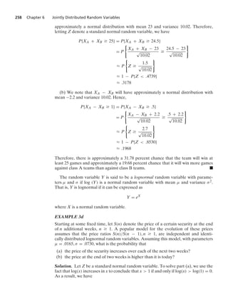
281. 266 Chapter 6 Jointly Distributed Random Variables
P(o|X = k) =
P(o, X = k)
P(X = k)
=
P(o)
P(X = k)
=
pk(1 − p)n−k
n
k
pk(1 − p)n−k
=
1
n
k
.
6.5 CONDITIONAL DISTRIBUTIONS: CONTINUOUS CASE
If X and Y have a joint probability density function f(x, y), then the conditional prob-
ability density function of X given that Y = y is defined, for all values of y such that
fY(y) 0, by
fX|Y(x|y) =
f(x, y)
fY(y)
To motivate this definition, multiply the left-hand side by dx and the right-hand side
by (dx dy)/dy to obtain
fX|Y(x|y) dx =
f(x, y) dx dy
fY(y) dy
L
P{x … X … x + dx, y … Y … y + dy}
P{y … Y … y + dy}
= P{x … X … x + dx|y … Y … y + dy}
In other words, for small values of dx and dy, fX|Y(x|y)dx represents the conditional
probability that X is between x and x + dx given that Y is between y and y + dy.
The use of conditional densities allows us to define conditional probabilities of
events associated with one random variable when we are given the value of a second
random variable. That is, if X and Y are jointly continuous, then, for any set A,
P{X ∈ A|Y = y} =
*
A
fX|Y(x|y) dx
In particular, by letting A = (−q, a], we can define the conditional cumulative distri-
bution function of X given that Y = y by
FX|Y(a|y) K P{X … a|Y = y} =
* a
−q
fX|Y(x|y) dx
The reader should note that, by using the ideas presented in the preceding discussion,
we have been able to give workable expressions for conditional probabilities, even
though the event on which we are conditioning (namely, the event {Y = y}) has
probability 0.
EXAMPLE 5a
The joint density of X and Y is given by
f(x, y) =
0
12
5 x(2 − x − y) 0 x 1, 0 y 1
0 otherwise
Compute the conditional density of X given that Y = y, where 0 y 1.

282. Section 6.5 Conditional Distributions: Continuous Case 267
Solution. For 0 x 1, 0 y 1, we have
fX|Y(x|y) =
f(x, y)
fY(y)
=
f(x, y)
- q
−q f(x, y) dx
=
x(2 − x − y)
- 1
0 x(2 − x − y) dx
=
x(2 − x − y)
2
3 − y/2
=
6x(2 − x − y)
4 − 3y .
EXAMPLE 5b
Suppose that the joint density of X and Y is given by
f(x, y) =
⎧
⎪
⎨
⎪
⎩
e−x/ye−y
y
0 x q, 0 y q
0 otherwise
Find P{X 1|Y = y}.
Solution. We first obtain the conditional density of X given that Y = y.
fX|Y(x|y) =
f(x, y)
fY(y)
=
e−x/ye−y/y
e−y
- q
0 (1/y)e−x/y dx
=
1
y
e−x/y
Hence,
P{X 1|Y = y} =
* q
1
1
y
e−x/y
dx
= −e−x/y
6
6
6
q
1
= e−1/y
.
If X and Y are independent continuous random variables, the conditional density
of X given that Y = y is just the unconditional density of X. This is so because, in the
independent case,
fX|Y(x|y) =
f(x, y)
fY(y)
=
fX(x)fY(y)
fY(y)
= fX(x)
We can also talk about conditional distributions when the random variables are nei-
ther jointly continuous nor jointly discrete. For example, suppose that X is a continu-
ous random variable having probability density function f and N is a discrete random
variable, and consider the conditional distribution of X given that N = n. Then

283. 268 Chapter 6 Jointly Distributed Random Variables
P{x X x + dx|N = n}
dx
=
P{N = n|x X x + dx}
P{N = n}
P{x X x + dx}
dx
and letting dx approach 0 gives
lim
dx→0
P{x X x + dx|N = n}
dx
=
P{N = n|X = x}
P{N = n}
f(x)
thus showing that the conditional density of X given that N = n is given by
fX|N(x|n) =
P{N = n|X = x}
P{N = n}
f(x)
EXAMPLE 5c The Bivariate Normal Distribution
One of the most important joint distributions is the bivariate normal distribution.
We say that the random variables X, Y have a bivariate normal distribution if, for
constants μx, μy, σx 0, σy 0, −1 ρ 1, their joint density function is given,
for all −q x, y q, by
f(x, y) =
1
2πσxσy
.
1 − ρ2
exp
⎧
⎨
⎩
−
1
2(1 − ρ2)
x − μx
σx
2
+
y − μy
σy
2
− 2ρ
(x − μx)(y − μy)
σxσy
⎤
⎦
⎫
⎪
⎬
⎪
⎭
We now determine the conditional density of X given that Y = y. In doing so, we
will continually collect all factors that do not depend on x and represent them by the
constants Ci. The final constant will then be found by using that
- q
−q fX|Y(x|y) dx = 1.
We have
fX|Y(x|y) =
f(x, y)
fY(y)
= C1f(x, y)
= C2 exp
⎧
⎨
⎩
−
1
2(1 − ρ2)
x − μx
σx
2
− 2ρ
x(y − μy)
σxσy
⎫
⎬
⎭
= C3 exp
⎧
⎪
⎨
⎪
⎩
−
1
2σ2
x (1 − ρ2)
⎡
⎣x2
− 2x
μx + ρ
σx
σy
(y − μy)
⎤
⎦
⎫
⎪
⎬
⎪
⎭
= C4 exp
⎧
⎪
⎨
⎪
⎩
−
1
2σ2
x (1 − ρ2)
⎡
⎣x −
μx + ρ
σx
σy
(y − μy)
⎤
⎦
2
⎫
⎪
⎬
⎪
⎭
Recognizing the preceding equation as a normal density, we can conclude that, given
Y = y, the random variable X is normally distributed with mean μx + ρ σx
σy
(y − μy)
and variance σ2
x (1 − ρ2). Also, because the joint density of Y, X is exactly the same as
that of X, Y, except that μx, σx are interchanged with μy, σy, it similarly follows that

284. Section 6.5 Conditional Distributions: Continuous Case 269
the conditional distribution of Y given X = x is the normal distribution with mean
μy + ρ
σy
σx
(x − μx) and variance σ2
y (1 − ρ2). It follows from these results that the
necessary and sufficient condition for the bivariate normal random variables X and
Y to be independent is that ρ = 0 (a result that also follows directly from their joint
density, because it is only when ρ = 0 that the joint density factors into two terms,
one depending only on x and the other only on y).
With C = 1
2πσxσy
√
1−ρ2
, the marginal density of X can be obtained from
fX(x) =
* q
−q
f(x, y) dy
= C
* q
−q
exp
⎧
⎪
⎨
⎪
⎩
−
1
2(1 − ρ2)
⎡
⎣
x − μx
σx
2
+
y − μy
σy
2
−2ρ
(x − μx)(y − μy)
σxσy
⎫
⎬
⎭
dy
Making the change of variables w =
y−μy
σy
gives
fX(x) = Cσy exp
0
−
1
2(1 − ρ2)
x − μx
σx
2
7
*
* q
−q
exp
0
−
1
2(1 − ρ2)
w2
− 2ρ
x − μx
σx
w
7
dw
= Cσy exp
0
−
1
2(1 − ρ2)
x − μx
σx
2
(1 − ρ2
)
7
*
* q
−q
exp
0
−
1
2(1 − ρ2)
w − ρ
x − μx
σx
2
7
dw
Because
1
.
2π(1 − ρ2)
* q
−q
exp
0
−
1
2(1 − ρ2)
w −
ρ
σx
(x − μx)
2
7
dw = 1
we see that
fX(x) = Cσy
8
2π(1 − ρ2) e−(x−μx)2/2σ2
x
=
1
√
2πσx
e−(x−μx)2/2σ2
x
That is, X is normal with mean μx and variance σ2
x . Similarly, Y is normal with
mean μy and variance σ2
y . .
EXAMPLE 5d
Consider n + m trials having a common probability of success. Suppose, however,
that this success probability is not fixed in advance but is chosen from a uniform (0, 1)

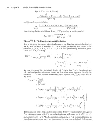
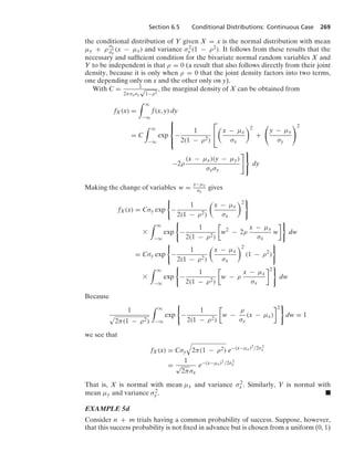
285. 270 Chapter 6 Jointly Distributed Random Variables
population. What is the conditional distribution of the success probability given that
the n + m trials result in n successes?
Solution. If we let X denote the probability that a given trial is a success, then X
is a uniform (0, 1) random variable. Also, given that X = x, the n + m trials are
independent with common probability of success x, so N, the number of successes,
is a binomial random variable with parameters (n + m, x). Hence, the conditional
density of X given that N = n is
fX|N(x|n) =
P{N = n|X = x}fX(x)
P{N = n}
=
n + m
n
xn(1 − x)m
P{N = n}
0 x 1
= cxn
(1 − x)m
where c does not depend on x. Thus, the conditional density is that of a beta random
variable with parameters n + 1, m + 1.
The preceding result is quite interesting, for it states that if the original or prior
(to the collection of data) distribution of a trial success probability is uniformly dis-
tributed over (0, 1) [or, equivalently, is beta with parameters (1, 1)] then the posterior
(or conditional) distribution given a total of n successes in n + m trials is beta with
parameters (1 + n, 1 + m). This is valuable, for it enhances our intuition as to what
it means to assume that a random variable has a beta distribution. .
∗6.6 ORDER STATISTICS
Let X1, X2, ... , Xn be n independent and identically distributed continuous random
variables having a common density f and distribution function F. Define
X(1) = smallest of X1, X2, ... , Xn
X(2) = second smallest of X1, X2, ... , Xn
#
#
#
X(j) = jth smallest of X1, X2, ... , Xn
#
#
#
X(n) = largest of X1, X2, ... , Xn
The ordered values X(1) … X(2) … · · · … X(n) are known as the order statistics cor-
responding to the random variables X1, X2, ... , Xn. In other words, X(1), ... , X(n) are
the ordered values of X1, ... , Xn.
The joint density function of the order statistics is obtained by noting that the order
statistics X(1), ... , X(n) will take on the values x1 … x2 … · · · … xn if and only if, for
some permutation (i1, i2, ... , in) of (1, 2, ... , n),
X1 = xi1
, X2 = xi2 , ... , Xn = xin

286. Section 6.6 Order Statistics 271
Since, for any permutation (i1, ... , in) of (1, 2, ... , n),
P
%
xi1
−
ε
2
X1 xi1
+
ε
2
, ... , xin −
ε
2
Xn xin +
ε
2
/
L εn
fX1
, · · · , Xn(xi1
, ... , xin )
= εn
f(xi1
) · · · f(xin )
= εn
f(x1) · · · f(xn)
it follows that, for x1 x2 · · · xn,
P
%
x1 −
ε
2
X(1) x1 +
ε
2
, ... , xn −
ε
2
X(n) xn +
ε
2
/
L n! εn
f(x1) · · · f(xn)
Dividing by εn and letting ε→0 yields
fX(1),...,X(n) (x1, x2, ... , xn) = n!f(x1) · · · f(xn) x1 x2 · · · xn (6.1)
Equation (6.1) is most simply explained by arguing that, in order for the vector
X(1), ... , X(n) to equal x1, ... , xn , it is necessary and sufficient for X1, ... , Xn to
equal one of the n! permutations of x1, ... , xn . Since the probability (density) that
X1, ... , Xn equals any given permutation of x1, ... , xn is just f(x1) · · · f(xn), Equa-
tion (6.1) follows.
EXAMPLE 6a
Along a road 1 mile long are 3 people “distributed at random.” Find the probability
that no 2 people are less than a distance of d miles apart when d … 1
2 .
Solution. Let us assume that “distributed at random” means that the positions of the
3 people are independent and uniformly distributed over the road. If Xi denotes the
position of the ith person, then the desired probability is P{X(i) X(i−1) + d, i =
2, 3}. Because
fX(1),X(2),X(3) (x1, x2, x3) = 3! 0 x1 x2 x3 1
it follows that
P{X(i) X(i−1) + d, i = 2, 3} =
* * *
xixj−1+d
fX(1),X(2),X(3) (x1, x2, x3) dx1 dx2 dx3
= 3!
* 1−2d
0
* 1−d
x1+d
* 1
x2+d
dx3 dx2 dx1
= 6
* 1−2d
0
* 1−d
x1+d
(1 − d − x2) dx2 dx1
= 6
* 1−2d
0
* 1−2d−x1
0
y2 dy2 dx1

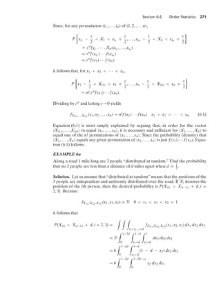
287. 272 Chapter 6 Jointly Distributed Random Variables
where we have made the change of variables y2 = 1 − d − x2. Continuing the string
of equalities yields
= 3
* 1−2d
0
(1 − 2d − x1)2
dx1
= 3
* 1−2d
0
y2
1 dy1
= (1 − 2d)3
Hence, the desired probability that no 2 people are within a distance d of each other
when 3 people are uniformly and independently distributed over an interval of size
1 is (1 − 2d)3 when d … 1
2 . In fact, the same method can be used to prove that
when n people are distributed at random over the unit interval, the desired
probability is
[1 − (n − 1)d]n
when d …
1
n − 1
The proof is left as an exercise. .
The density function of the jth-order statistic X(j) can be obtained either by inte-
grating the joint density function (6.1) or by direct reasoning as follows: In order for
X(j) to equal x, it is necessary for j − 1 of the n values X1, ... , Xn to be less than
x, n − j of them to be greater than x, and 1 of them to equal x. Now, the probability
density that any given set of j − 1 of the Xi’s are less than x, another given set of
n − j are all greater than x, and the remaining value is equal to x equals
[F(x)]j−1
[1 − F(x)]n−j
f(x)
Hence, since there are
n
j − 1, n − j, 1
=
n!
(n − j)!(j − 1)!
different partitions of the n random variables X1, ... , Xn into the preceding three
groups, it follows that the density function of X(j) is given by
fX(j) (x) =
n!
(n − j)!(j − 1)!
[F(x)]j−1
[1 − F(x)]n−j
f(x) (6.2)
EXAMPLE 6b
When a sample of 2n + 1 random variables (that is, when 2n + 1 independent and
identically distributed random variables) is observed, the (n + 1)st smallest is called
the sample median. If a sample of size 3 from a uniform distribution over (0, 1) is
observed, find the probability that the sample median is between 1
4 and 3
4 .
Solution. From Equation (6.2), the density of X(2) is given by
fX(2) (x) =
3!
1!1!
x(1 − x) 0 x 1

288. Section 6.6 Order Statistics 273
Hence,
P
%
1
4
X(2)
3
4
/
= 6
* 3/4
1/4
x(1 − x) dx
= 6
0
x2
2
−
x3
3
76
6
6
6
6
6
x=3/4
x=1/4
=
11
16
.
The cumulative distribution function of X(j) can be found by integrating Equa-
tion (6.2). That is,
FX(j) (y) =
n!
(n − j)!(j − 1)!
* y
−q
[F(x)]j−1
[1 − F(x)]n−j
f(x) dx (6.3)
However, FX(j) (y) could also have been derived directly by noting that the jth order
statistic is less than or equal to y if and only if there are j or more of the Xi’s that are
less than or equal to y. Thus, because the number of Xi’s that are less than or equal
to y is a binomial random variable with parameters n, p = F(y), it follows that
FX(j) (y) = P{X(j) … y} = P{j or more of the Xi’s are … y}
=
n
k=j
n
k
[F(y)]k
[1 − F(y)]n−k
(6.4)
If, in Equations (6.3) and (6.4), we take F to be the uniform (0, 1) distribution [that
is, f(x) = 1, 0 x 1], then we obtain the interesting analytical identity
n
k=j
n
k
yk
(1 − y)n−k
=
n!
(n − j)!(j − 1)!
* y
0
xj−1
(1 − x)n−j
dx 0 … y … 1 (6.5)
By employing the same type of argument that we used in establishing
Equation (6.2), we can show that the joint density function of the order statistics X(i)
and X(j) when i j is
fX(i),X(j) (xi, xj) =
n!
(i − 1)!(j − i − 1)!(n − j)!
[F(xi)]i−1
(6.6)
* [F(xj) − F(xi)]j−i−1
[1 − F(xj)]n−j
f(xi)f(xj)
for all xi xj.
EXAMPLE 6c Distribution of the range of a random sample
Suppose that n independent and identically distributed random variables X1, X2, ... ,
Xn are observed. The random variable R defined by R = X(n) − X(1) is called the
range of the observed random variables. If the random variables Xi have distribution
function F and density function f, then the distribution of R can be obtained from
Equation (6.6) as follows: For a Ú 0,

289. 274 Chapter 6 Jointly Distributed Random Variables
P{R … a} = P{X(n) − X(1) … a}
=
* *
xn−x1…a
fX(1),X(n) (x1, xn) dx1 dxn
=
* q
−q
* x1+a
x1
n!
(n − 2)!
[F(xn) − F(x1)]n−2
f(x1)f(xn) dxn dx1
Making the change of variable y = F(xn) − F(x1), dy = f(xn) dxn yields
* x1+a
x1
[F(xn) − F(x1)]n−2
f(xn) dxn =
* F(x1+a)−F(x1)
0
yn−2
dy
=
1
n − 1
[F(x1 + a) − F(x1)]n−1
Thus,
P{R … a} = n
* q
−q
[F(x1 + a) − F(x1)]n−1
f(x1) dx1 (6.7)
Equation (6.7) can be evaluated explicitly only in a few special cases. One such case
is when the Xi’s are all uniformly distributed on (0, 1). In this case, we obtain, from
Equation (6.7), that for 0 a 1,
P{R a} = n
* 1
0
[F(x1 + a) − F(x1)]n−1
f(x1) dx1
= n
* 1−a
0
an−1
dx1 + n
* 1
1−a
(1 − x1)n−1
dx1
= n(1 − a)an−1
+ an
Differentiation yields the density function of the range: given in this case by
fR(a) =
0
n(n − 1)an−2(1 − a) 0 … a … 1
0 otherwise
That is, the range of n independent uniform (0, 1) random variables is a beta random
variable with parameters n − 1, 2. .
6.7 JOINT PROBABILITY DISTRIBUTION OF FUNCTIONS OF RANDOM VARIABLES
Let X1 and X2 be jointly continuous random variables with joint probability density
function fX1,X2 . It is sometimes necessary to obtain the joint distribution of the ran-
dom variables Y1 and Y2, which arise as functions of X1 and X2. Specifically, suppose
that Y1 = g1(X1, X2) and Y2 = g2(X1, X2) for some functions g1 and g2.
Assume that the functions g1 and g2 satisfy the following conditions:
1. The equations y1 = g1(x1, x2) and y2 = g2(x1, x2) can be uniquely solved for x1
and x2 in terms of y1 and y2, with solutions given by, say, x1 = h1(y1, y2), x2 =
h2(y1, y2).
2. The functions g1 and g2 have continuous partial derivatives at all points (x1, x2)
and are such that the 2 * 2 determinant

290. Section 6.7 Joint Distribution of Functions of Random Variables 275
J(x1, x2) =
6
6
6
6
6
6
6
6
6
∂g1
∂x1
∂g1
∂x2
∂g2
∂x1
∂g2
∂x2
6
6
6
6
6
6
6
6
6
K
∂g1
∂x1
∂g2
∂x2
−
∂g1
∂x2
∂g2
∂x1
Z 0
at all points (x1, x2).
Under these two conditions, it can be shown that the random variables Y1 and Y2
are jointly continuous with joint density function given by
fY1Y2 (y1, y2) = fX1,X2 (x1, x2)|J(x1, x2)|−1
(7.1)
where x1 = h1(y1, y2), x2 = h2(y1, y2).
A proof of Equation (7.1) would proceed along the following lines:
P{Y1 … y1, Y2 … y2} =
* *
(x1, x2) :
g1(x1, x2) … y1
g2(x1, x2) … y2
fX1,X2 (x1, x2) dx1 dx2 (7.2)
The joint density function can now be obtained by differentiating Equation (7.2) with
respect to y1 and y2. That the result of this differentiation will be equal to the right-
hand side of Equation (7.1) is an exercise in advanced calculus whose proof will not
be presented in this book.
EXAMPLE 7a
Let X1 and X2 be jointly continuous random variables with probability density func-
tion fX1,X2 . Let Y1 = X1 + X2, Y2 = X1 − X2. Find the joint density function of Y1
and Y2 in terms of fX1,X2 .
Solution. Let g1(x1, x2) = x1 + x2 and g2(x1, x2) = x1 − x2. Then
J(x1, x2) =
6
6
6
6
1 1
1 −1
6
6
6
6 = −2
Also, since the equations y1 = x1 + x2 and y2 = x1 − x2 have x1 = (y1 + y2)/2, x2 =
(y1 − y2)/2 as their solution, it follows from Equation (7.1) that the desired density is
fY1,Y2 (y1, y2) =
1
2
fX1,X2
y1 + y2
2
,
y1 − y2
2
For instance, if X1 and X2 are independent uniform (0, 1) random variables, then
fY1,Y2 (y1, y2) =
0
1
2 0 … y1 + y2 … 2, 0 … y1 − y2 … 2
0 otherwise

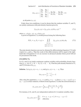
291. 276 Chapter 6 Jointly Distributed Random Variables
or if X1 and X2 are independent exponential random variables with respective param-
eters λ1 and λ2, then
fY1,Y2 (y1, y2)
=
⎧
⎪
⎪
⎨
⎪
⎪
⎩
λ1λ2
2
exp
0
−λ1
y1 + y2
2
− λ2
y1 − y2
2
7
y1 + y2 Ú 0, y1 − y2 Ú 0
0 otherwise
Y
X
R
⍜
FIGURE 6.4: • = Random point. (X, Y) = (R, Θ).
Finally, if X1 and X2 are independent standard normal random variables, then
fY1,Y2 (y1, y2) =
1
4π
e−[(y1+y2)2/8+(y1−y2)2/8]
=
1
4π
e−(y2
1+y2
2)/4
=
1
√
4π
e−y2
1/4 1
√
4π
e−y2
2/4
Thus, not only do we obtain (in agreement with Proposition 3.2) that both X1 + X2
and X1 − X2 are normal with mean 0 and variance 2, but we also conclude that these
two random variables are independent. (In fact, it can be shown that if X1 and X2
are independent random variables having a common distribution function F, then
X1 + X2 will be independent of X1 − X2 if and only if F is a normal distribution
function.) .
EXAMPLE 7b
Let (X, Y) denote a random point in the plane, and assume that the rectangular
coordinates X and Y are independent standard normal random variables. We are
interested in the joint distribution of R, Θ, the polar coordinate representation of
(x, y). (See Figure 6.4.)
Suppose first that X and Y are both positive. For x and y positive, letting r =
g1(x, y) =
.
x2 + y2 and θ = g2(x, y) = tan−1 y/x, we see that
∂g1
∂x
=
x
.
x2 + y2
∂g1
∂y
=
y
.
x2 + y2

292. Section 6.7 Joint Distribution of Functions of Random Variables 277
∂g2
∂x
=
1
1 + (y/x)2
−y
x2
=
−y
x2 + y2
∂g2
∂y
=
1
x[1 + (y/x)2]
=
x
x2 + y2
Hence,
J(x, y) =
x2
(x2 + y2)3/2
+
y2
(x2 + y2)3/2
=
1
.
x2 + y2
=
1
r
Because the conditional joint density function of X, Y given that they are both
positive is
f(x, y|X 0, Y 0) =
f(x, y)
P(X 0, Y 0)
=
2
π
e−(x2+y2)/2
, x 0, y 0
we see that the conditional joint density function of R =
.
X2 + Y2 and =
tan−1(Y/X), given that X and Y are both positive, is
f(r, θ|X 0, Y 0) =
2
π
re−r2/2
, 0 θ π/2, 0 r q
Similarly, we can show that
f(r, θ|X 0, Y 0) =
2
π
re−r2/2
, π/2 θ π, 0 r q
f(r, θ|X 0, Y 0) =
2
π
re−r2/2
, π θ 3π/2, 0 r q
f(r, θ|X 0, Y 0) =
2
π
re−r2/2
, 3π/2 θ 2π, 0 r q
As the joint density is an equally weighted average of these 4 conditional joint densi-
ties, we obtain that the joint density of R, Θ is given by
f(r, θ) =
1
2π
re−r2/2
0 θ 2π, 0 r q
Now, this joint density factors into the marginal densities for R and Θ, so R and Θ
are independent random variables, with Θ being uniformly distributed over (0, 2π)
and R having the Rayleigh distribution with density
f(r) = re−r2/2
0 r q
(For instance, when one is aiming at a target in the plane, if the horizontal and vertical
miss distances are independent standard normals, then the absolute value of the error
has the preceding Rayleigh distribution.)
This result is quite interesting, for it certainly is not evident a priori that a ran-
dom vector whose coordinates are independent standard normal random variables
will have an angle of orientation that not only is uniformly distributed, but also is
independent of the vector’s distance from the origin.

293. 278 Chapter 6 Jointly Distributed Random Variables
If we wanted the joint distribution of R2 and Θ, then, since the transformation
d = g1(x, y) = x2 + y2 and θ = g2(x, y) = tan−1 y/x has the Jacobian
J =
6
6
6
6
6
6
6
2x 2y
−y
x2 + y2
x
x2 + y2
6
6
6
6
6
6
6
= 2
it follows that
f(d, θ) =
1
2
e−d/2 1
2π
0 d q, 0 θ 2π
Therefore, R2 and Θ are independent, with R2 having an exponential distribution
with parameter 1
2. But because R2 = X2 + Y2, it follows by definition that R2 has
a chi-squared distribution with 2 degrees of freedom. Hence, we have a verification
of the result that the exponential distribution with parameter 1
2 is the same as the
chi-squared distribution with 2 degrees of freedom.
The preceding result can be used to simulate (or generate) normal random vari-
ables by making a suitable transformation on uniform random variables. Let U1 and
U2 be independent random variables, each uniformly distributed over (0, 1). We will
transform U1, U2 into two independent unit normal random variables X1 and X2
by first considering the polar coordinate representation (R, Θ) of the random vec-
tor (X1, X2). From the preceding, R2 and Θ will be independent, and, in addition,
R2 = X2
1 + X2
2 will have an exponential distribution with parameter λ = 1
2. But
−2 log U1 has such a distribution, since, for x 0,
P{−2 log U1 x} = P
%
log U1 −
x
2
/
= P{U1 e−x/2
}
= 1 − e−x/2
Also, because 2πU2 is a uniform (0, 2π) random variable, we can use it to generate Θ.
That is, if we let
R2
= −2 log U1
Θ = 2πU2
then R2 can be taken to be the square of the distance from the origin and θ can be
taken to be the angle of orientation of (X1, X2). Now, since X1 = R cos Θ, X2 =
R sin Θ, it follows that
X1 =
.
−2 log U1 cos(2πU2)
X2 =
.
−2 log U1 sin(2πU2)
are independent standard normal random variables. .
EXAMPLE 7c
If X and Y are independent gamma random variables with parameters (α, λ) and
(β, λ), respectively, compute the joint density of U = X + Y and V = X/(X + Y).

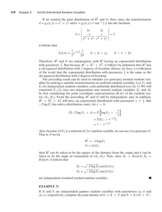
294. Section 6.7 Joint Distribution of Functions of Random Variables 279
Solution. The joint density of X and Y is given by
fX,Y(x, y) =
λe−λx(λx)α−1
(α)
λe−λy(λy)β−1
(β)
=
λα+β
(α)(β)
e−λ(x+y)
xα−1
yβ−1
Now, if g1(x, y) = x + y, g2(x, y) = x/(x + y), then
∂g1
∂x
=
∂g1
∂y
= 1
∂g2
∂x
=
y
(x + y)2
∂g2
∂y
= −
x
(x + y)2
so
J(x, y) =
6
6
6
6
6
6
6
1 1
y
(x + y)2
−x
(x + y)2
6
6
6
6
6
6
6
= −
1
x + y
Finally, as the equations u = x + y, v = x/(x + y) have as their solutions x = uv, y =
u(1 − v), we see that
fU,V(u, v) = fX,Y[uv, u(1 − v)]u
=
λe−λu(λu)α+β−1
(α + β)
vα−1(1 − v)β−1(α + β)
(α)(β)
Hence, X + Y and X/(X + Y) are independent, with X + Y having a gamma dis-
tribution with parameters (α + β, λ) and X/(X + Y) having a beta distribution with
parameters (α, β). The preceding reasoning also shows that B(α, β), the normalizing
factor in the beta density, is such that
B(α, β) K
* 1
0
vα−1
(1 − v)β−1
dv
=
(α)(β)
(α + β)
This entire result is quite interesting. For suppose there are n + m jobs to be per-
formed, each (independently) taking an exponential amount of time with rate λ to be
completed and suppose that we have two workers to perform these jobs. Worker I
will do jobs 1, 2, ... , n, and worker II will do the remaining m jobs. If we let X and Y
denote the total working times of workers I and II, respectively, then (either from the
foregoing result or from Example 3b) X and Y will be independent gamma random
variables having parameters (n, λ) and (m, λ), respectively. It then follows that, inde-
pendently of the working time needed to complete all n + m jobs (that is, of X + Y),
the proportion of this work that will be performed by worker I has a beta distribution
with parameters (n, m). .
When the joint density function of the n random variables X1, X2, ... , Xn is given
and we want to compute the joint density function of Y1, Y2, ... , Yn, where
Y1 = g1(X1, ... , Xn) Y2 = g2(X1, ... , Xn), ... Yn = gn(X1, ... , Xn)

295. 280 Chapter 6 Jointly Distributed Random Variables
the approach is the same—namely, we assume that the functions gi have continuous
partial derivatives and that the Jacobian determinant.
J(x1, ... , xn) =
6
6
6
6
6
6
6
6
6
6
6
6
6
6
∂g1
∂x1
∂g1
∂x2
· · ·
∂g1
∂xn
∂g2
∂x1
∂g2
∂x2
· · ·
∂g2
∂xn
∂gn
∂x1
∂gn
∂x2
· · ·
∂gn
∂xn
6
6
6
6
6
6
6
6
6
6
6
6
6
6
Z 0
at all points (x1, ... , xn). Furthermore, we suppose that the equations y1 =
g1(x1, ... , xn), y2 = g2(x1, ... , xn), ... , yn = gn(x1, ... , xn) have a unique solution, say,
x1 = h1(y1, ... , yn), ... , xn = hn(y1, ... , yn). Under these assumptions, the joint den-
sity function of the random variables Yi is given by
fY1,...,Yn (y1, ... , yn) = fX1,...,Xn (x1, ... , xn)|J(x1, ... , xn)|−1
(7.3)
where xi = hi(y1, ... , yn), i = 1, 2, ... , n.
EXAMPLE 7d
Let X1, X2, and X3 be independent standard normal random variables. If Y1 = X1 +
X2 + X3, Y2 = X1 − X2, and Y3 = X1 − X3, compute the joint density function of
Y1, Y2, Y3.
Solution. Letting Y1 = X1 + X2 + X3, Y2 = X1 − X2, Y3 = X1 − X3, the Jacobian
of these transformations is given by
J =
6
6
6
6
6
6
1 1 1
1 −1 0
1 0 −1
6
6
6
6
6
6
= 3
As the preceding transformations yield that
X1 =
Y1 + Y2 + Y3
3
X2 =
Y1 − 2Y2 + Y3
3
X3 =
Y1 + Y2 − 2Y3
3
we see from Equation (7.3) that
fY1, Y2, Y3 (y1, y2, y3)
=
1
3
fX1, X2, X3
y1 + y2 + y3
3
,
y1 − 2y2 + y3
3
,
y1 + y2 − 2y3
3
Hence, as
fX1, X2, X3 (x1, x2, x3) =
1
(2π)3/2
e− 3
i=1 x2
i /2
we see that
fY1, Y2, Y3 (y1, y2, y3) =
1
3(2π)3/2
e−Q(y1, y2, y3)/2

296. Section 6.7 Joint Distribution of Functions of Random Variables 281
where
Q(y1, y2, y3)
=
y1 + y2 + y3
3
2
+
y1 − 2y2 + y3
3
2
+
y1 + y2 − 2y3
3
2
=
y2
1
3
+
2
3
y2
2 +
2
3
y2
3 −
2
3
y2y3
.
EXAMPLE 7e
Let X1, X2, ... , Xn be independent and identically distributed exponential random
variables with rate λ. Let
Yi = X1 + · · · + Xi i = 1, ... , n
(a) Find the joint density function of Y1, ... , Yn.
(b) Use the result of part (a) to find the density of Yn.
Solution. (a) The Jacobian of the transformations Y1 = X1, Y2 = X1 + X2, ...,
Yn = X1 + · · · + Xn is
J =
6
6
6
6
6
6
6
6
6
6
6
6
1 0 0 0 · · · 0
1 1 0 0 · · · 0
1 1 1 0 · · · 0
· · · · · ·
· · · · · ·
1 1 1 1 · · · 1
6
6
6
6
6
6
6
6
6
6
6
6
Since only the first term of the determinant will be nonzero, we have J = 1.
Now, the joint density function of X1, ... , Xn is given by
fX1,...,Xn (x1, ... , xn) =
n
i=1
λe−λxi 0 xi q, i = 1, ... , n
Hence, because the preceding transformations yield
X1 = Y1, X2 = Y2 − Y1, ... , Xi = Yi − Yi−1, ... , Xn = Yn − Yn−1
it follows from Equation (7.3) that the joint density function of Y1, ... , Yn is
fY1,...,Yn (y1, y2, ... , yn)
= fX1,...,Xn (y1, y2 − y1, ... , yi − yi−1, ... , yn − yn−1)
= λn
exp
⎧
⎪
⎨
⎪
⎩
−λ
⎡
⎣y1 +
n
i=2
(yi − yi−1)
⎤
⎦
⎫
⎪
⎬
⎪
⎭
= λn
e−λyn 0 y1, 0 yi − yi−1, i = 2, ... , n
= λn
e−λyn 0 y1 y2 · · · yn

297. 282 Chapter 6 Jointly Distributed Random Variables
(b) To obtain the marginal density of Yn, let us integrate out the other variables one
at a time. Doing this gives
fY2,...,Yn (y2, ... , yn) =
* y2
0
λn
e−λyn dy1
= λn
y2e−λyn 0 y2 y3 · · · yn
Continuing, we obtain
fY3,...,Yn (y3, ... , yn) =
* y3
0
λn
y2e−λyn dy2
= λn y2
3
2
e−λyn 0 y3 y4 · · · yn
The next integration yields
fY4,...,Yn (y4, ... , yn) = λn y3
4
3!
e−λyn 0 y4 · · · yn
Continuing in this fashion gives
fYn (yn) = λn yn−1
n
(n − 1)!
e−λyn 0 yn
which, in agreement with the result obtained in Example 3b, shows that X1 +
· · · + Xn is a gamma random variable with parameters n and λ. .
∗6.8 EXCHANGEABLE RANDOM VARIABLES
The random variables X1, X2, ... , Xn are said to be exchangeable if, for every permu-
tation i1, ... , in of the integers 1, ... , n,
P{Xi1
… x1, Xi2 … x2, ... , Xin … xn} = P{X1 … x1, X2 … x2, ... , Xn … xn}
for all x1, ... , xn. That is, the n random variables are exchangeable if their joint distri-
bution is the same no matter in which order the variables are observed.
Discrete random variables will be exchangeable if
P{Xi1
= x1, Xi2 = x2, ... , Xin = xn} = P{X1 = x1, X2 = x2, ... , Xn = xn}
for all permutations i1, ... , in, and all values x1, ... , xn. This is equivalent to stating
that p(x1, x2, ... , xn) = P{X1 = x1, ... , Xn = xn} is a symmetric function of the vector
(x1, ... , xn), which means that its value does not change when the values of the vector
are permuted.
EXAMPLE 8a
Suppose that balls are withdrawn one at a time and without replacement from an
urn that initially contains n balls, of which k are considered special, in such a manner
that each withdrawal is equally likely to be any of the balls that remain in the urn
at the time. Let Xi = 1 if the ith ball withdrawn is special and let Xi = 0 otherwise.
We will show that the random variables X1, ... , Xn are exchangeable. To do so, let
(x1, ... , xn) be a vector consisting of k ones and n − k zeros. However, before consid-
ering the joint mass function evaluated at (x1, ... , xn), let us try to gain some insight by

298. Section 6.8 Exchangeable Random Variables 283
considering a fixed such vector—for instance, consider the vector (1, 1, 0, 1, 0, ... , 0, 1),
which is assumed to have k ones and n − k zeros. Then
p(1, 1, 0, 1, 0, ... , 0, 1) =
k
n
k − 1
n − 1
n − k
n − 2
k − 2
n − 3
n − k − 1
n − 4
· · ·
1
2
1
1
which follows because the probability that the first ball is special is k/n, the condi-
tional probability that the next one is special is (k − 1)/(n − 1), the conditional
probability that the next one is not special is (n − k)/(n − 2), and so on. By the same
argument, it follows that p(x1, ... , xn) can be expressed as the product of n fractions.
The successive denominator terms of these fractions will go from n down to 1. The
numerator term at the location where the vector (x1, ... , xn) is 1 for the ith time is
k − (i − 1), and where it is 0 for the ith time it is n − k − (i − 1). Hence, since the
vector (x1, ... , xn) consists of k ones and n − k zeros, we obtain
p(x1, ... , xn) =
k!(n − k)!
n!
xi = 0, 1,
n
i=1
xi = k
Since this is a symmetric function of (x1, ... , xn), it follows that the random variables
are exchangeable. .
Remark. Another way to obtain the preceding formula for the joint probability
mass function is to regard all the n balls as distinguishable from each other. Then,
since the outcome of the experiment is an ordering of these balls, it follows that
there are n! equally likely outcomes. Finally, because the number of outcomes hav-
ing special and nonspecial balls in specified places is equal to the number of ways of
permuting the special and the nonspecial balls among themselves, namely k!(n − k)!,
we obtain the preceding density function. .
It is easily seen that if X1, X2, ... , Xn are exchangeable, then each Xi has the same
probability distribution. For instance, if X and Y are exchangeable discrete random
variables, then
P{X = x} =
y
P{X = x, Y = y} =
y
P{X = y, Y = x} = P{Y = x}
For example, it follows from Example 8a that the ith ball withdrawn will be special
with probability k/n, which is intuitively clear, since each of the n balls is equally
likely to be the ith one selected.
EXAMPLE 8b
In Example 8a, let Yi denote the selection number of the first special ball withdrawn,
let Y2 denote the additional number of balls that are then withdrawn until the second
special ball appears, and, in general, let Yi denote the additional number of balls
withdrawn after the (i − 1)st special ball is selected until the ith is selected, i =
1, ... , k. For instance, if n = 4, k = 2 and X1 = 1, X2 = 0, X3 = 0, X4 = 1, then
Y1 = 1, Y2 = 3. Now, Y1 = i1, Y2 = i2, ... , Yk = ik 3 Xi1
= Xi1+i2 = · · · =
Xi1+···+ik
= 1, Xj = 0, otherwise; thus, from the joint mass function of the Xi, we
obtain
P{Y1 = i1, Y2 = i2, ... , Yk = ik} =
k!(n − k)!
n!
i1 + · · · + ik … n
Hence, the random variables Y1, ... , Yk are exchangeable. Note that it follows from
this result that the number of cards one must select from a well-shuffled deck until

299. 284 Chapter 6 Jointly Distributed Random Variables
an ace appears has the same distribution as the number of additional cards one must
select after the first ace appears until the next one does, and so on. .
EXAMPLE 8c
The following is known as Polya’s urn model: Suppose that an urn initially contains n
red and m blue balls. At each stage, a ball is randomly chosen, its color is noted, and
it is then replaced along with another ball of the same color. Let Xi = 1 if the ith ball
selected is red and let it equal 0 if the ith ball is blue, i Ú 1. To obtain a feeling for the
joint probabilities of these Xi, note the following special cases:
P{X1 = 1, X2 = 1, X3 = 0, X4 = 1, X5 = 0}
=
n
n + m
n + 1
n + m + 1
m
n + m + 2
n + 2
n + m + 3
m + 1
n + m + 4
=
n(n + 1)(n + 2)m(m + 1)
(n + m)(n + m + 1)(n + m + 2)(n + m + 3)(n + m + 4)
and
P{X1 = 0, X2 = 1, X3 = 0, X4 = 1, X5 = 1}
=
m
n + m
n
n + m + 1
m + 1
n + m + 2
n + 1
n + m + 3
n + 2
n + m + 4
=
n(n + 1)(n + 2)m(m + 1)
(n + m)(n + m + 1)(n + m + 2)(n + m + 3)(n + m + 4)
By the same reasoning, for any sequence x1, ... , xk that contains r ones and k − r
zeros, we have
P{X1 = x1, ... , Xk = xk}
=
n(n + 1) · · · (n + r − 1)m(m + 1) · · · (m + k − r − 1)
(n + m) · · · (n + m + k − 1)
Therefore, for any value of k, the random variables X1, ... , Xk are exchangeable.
An interesting corollary of the exchangeability in this model is that the probability
that the ith ball selected is red is the same as the probability that the first ball selected
is red, namely, n
n+m. (For an intuitive argument for this initially nonintuitive result,
imagine that all the n + m balls initially in the urn are of different types. That is, one
is a red ball of type 1, one is a red ball of type 2, ..., one is a red ball type of n, one is
a blue ball of type 1, and so on, down to the blue ball of type m. Suppose that when
a ball is selected it is replaced along with another of its type. Then, by symmetry, the
ith ball selected is equally likely to be of any of the n + m distinct types. Because n
of these n + m types are red, the probability is n
n+m .) .
Our final example deals with continuous random variables that are exchangeable.
EXAMPLE 8d
Let X1, X2, ... , Xn be independent uniform (0, 1) random variables, and denote their
order statistics by X(1), ... , X(n). That is, X(j) is the jth smallest of X1, X2, ... , Xn.

300. Summary 285
Also, let
Y1 = X(1),
Yi = X(i) − X(i−1), i = 2, ... n
Show that Y1, ... , Yn are exchangeable.
Solution. The transformations
y1 = x1, ... , yi = xi − xi−1 i = 2, ... , n
yield
xi = y1 + · · · + yi i = 1, ... , n
As it is easy to see that the Jacobian of the preceding transformations is equal to 1,
so, from Equation (7.3), we obtain
fY1,...,Yn (y1, y2, ... , yn) = f(y1, y1 + y2, ... , y1 + · · · + yn)
where f is the joint density function of the order statistics. Hence, from Equation (6.1),
we obtain that
fY1,...,Yn (y1, y2, ... , yn) = n! 0 y1 y1 + y2 · · · y1 + · · · + yn 1
or, equivalently,
fY1,...,Yn (y1, y2, ... , yn) = n! 0 yi 1, i = 1, ... , n, y1 + · · · + yn 1
Because the preceding joint density is a symmetric function of y1, ... , yn, we see that
the random variables Y1, ... , Yn are exchangeable. .
SUMMARY
The joint cumulative probability distribution function of the pair of random variables
X and Y is defined by
F(x, y) = P{X … x, Y … y} − q x, y q
All probabilities regarding the pair can be obtained from F. To find the individual
probability distribution functions of X and Y, use
FX(x) = lim
y→q
F(x, y) FY(y) = lim
x→q
F(x, y)
If X and Y are both discrete random variables, then their joint probability mass
function is defined by
p(i, j) = P{X = i, Y = j}
The individual mass functions are
P{X = i} =
j
p(i, j) P{Y = j} =
i
p(i, j)
The random variables X and Y are said to be jointly continuous if there is a func-
tion f(x, y), called the joint probability density function, such that for any two-dimensional
set C,
P{(X, Y) ∈ C} =
* *
C
f(x, y) dx dy

301. 286 Chapter 6 Jointly Distributed Random Variables
It follows from the preceding formula that
P{x X x + dx, y Y y + dy} L f(x, y) dx dy
If X and Y are jointly continuous, then they are individually continuous with density
functions
fX(x) =
* q
−q
f(x, y)dy fY(y) =
* q
−q
f(x, y) dx
The random variables X and Y are independent if, for all sets A and B,
P{X ∈ A, Y ∈ B} = P{X ∈ A}P{Y ∈ B}
If the joint distribution function (or the joint probability mass function in the discrete
case, or the joint density function in the continuous case) factors into a part depending
only on x and a part depending only on y, then X and Y are independent.
In general, the random variables X1, ... , Xn are independent if, for all sets of real
numbers A1, ... , An,
P{X1 ∈ A1, ... , Xn ∈ An} = P{X1 ∈ A1} · · · P{Xn ∈ An}
If X and Y are independent continuous random variables, then the distribution func-
tion of their sum can be obtained from the identity
FX+Y(a) =
* q
−q
FX(a − y)fY(y)dy
If Xi, i = 1, ... , n, are independent normal random variables with respective param-
eters μi and σ2
i , i = 1, ... , n, then
n
i=1
Xi is normal with parameters
n
i=1
μi and
n
i=1
σ2
i .
If Xi, i = 1, ... , n, are independent Poisson random variables with respective param-
eters λi, i = 1, ... , n, then
n
i=1
Xi is Poisson with parameter
n
i=1
λi.
If X and Y are discrete random variables, then the conditional probability mass
function of X given that Y = y is defined by
P{X = x|Y = y} =
p(x, y)
pY(y)
where p is their joint probability mass function. Also, if X and Y are jointly continu-
ous with joint density function f, then the conditional probability density function of
X given that Y = y is given by
fX|Y(x|y) =
f(x, y)
fY(y)
The ordered values X(1) … X(2) … · · · … X(n) of a set of independent and identically
distributed random variables are called the order statistics of that set. If the random
variables are continuous and have density function f, then the joint density function
of the order statistics is
f(x1, ... , xn) = n!f(x1) · · · f(xn) x1 … x2 … · · · … xn
The random variables X1, ... , Xn are called exchangeable if the joint distribution of
Xi1
, ... , Xin is the same for every permutation i1, ... , in of 1, ... , n.

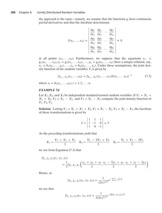
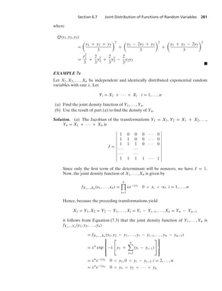
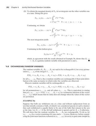
302. Problems 287
PROBLEMS
6.1. Two fair dice are rolled. Find the joint probability
mass function of X and Y when
(a) X is the largest value obtained on any die and
Y is the sum of the values;
(b) X is the value on the first die and Y is the
larger of the two values;
(c) X is the smallest and Y is the largest value
obtained on the dice.
6.2. Suppose that 3 balls are chosen without replace-
ment from an urn consisting of 5 white and 8 red
balls. Let Xi equal 1 if the ith ball selected is white,
and let it equal 0 otherwise. Give the joint proba-
bility mass function of
(a) X1, X2;
(b) X1, X2, X3.
6.3. In Problem 2, suppose that the white balls are
numbered, and let Yi equal 1 if the ith white ball is
selected and 0 otherwise. Find the joint probability
mass function of
(a) Y1, Y2;
(b) Y1, Y2, Y3.
6.4. Repeat Problem 2 when the ball selected is
replaced in the urn before the next selection.
6.5. Repeat Problem 3a when the ball selected is
replaced in the urn before the next selection.
6.6. A bin of 5 transistors is known to contain 2 that
are defective. The transistors are to be tested, one
at a time, until the defective ones are identified.
Denote by N1 the number of tests made until the
first defective is identified and by N2 the number of
additional tests until the second defective is identi-
fied. Find the joint probability mass function of N1
and N2.
6.7. Consider a sequence of independent Bernoulli tri-
als, each of which is a success with probability p.
Let X1 be the number of failures preceding the
first success, and let X2 be the number of failures
between the first two successes. Find the joint mass
function of X1 and X2.
6.8. The joint probability density function of X and Y
is given by
f(x, y) = c(y2
− x2
)e−y
− y … x … y, 0 y q
(a) Find c.
(b) Find the marginal densities of X and Y.
(c) Find E[X].
6.9. The joint probability density function of X and Y
is given by
f(x, y) =
6
7
x2
+
xy
2
0 x 1, 0 y 2
(a) Verify that this is indeed a joint density func-
tion.
(b) Compute the density function of X.
(c) Find P{X Y}.
(d) Find P{Y 1
2 |X 1
2 }.
(e) Find E[X].
(f) Find E[Y].
6.10. The joint probability density function of X and Y
is given by
f(x, y) = e−(x+y)
0 … x q, 0 … y q
Find (a) P{X Y} and (b) P{X a}.
6.11. A television store owner figures that 45 percent of
the customers entering his store will purchase an
ordinary television set, 15 percent will purchase
a plasma television set, and 40 percent will just
be browsing. If 5 customers enter his store on
a given day, what is the probability that he will
sell exactly 2 ordinary sets and 1 plasma set on
that day?
6.12. The number of people that enter a drugstore in
a given hour is a Poisson random variable with
parameter λ = 10. Compute the conditional prob-
ability that at most 3 men entered the drugstore,
given that 10 women entered in that hour. What
assumptions have you made?
6.13. A man and a woman agree to meet at a certain
location about 12:30 P.M. If the man arrives at
a time uniformly distributed between 12:15 and
12:45, and if the woman independently arrives at
a time uniformly distributed between 12:00 and 1
P.M., find the probability that the first to arrive
waits no longer than 5 minutes. What is the proba-
bility that the man arrives first?
6.14. An ambulance travels back and forth at a con-
stant speed along a road of length L. At a certain
moment of time, an accident occurs at a point uni-
formly distributed on the road. [That is, the dis-
tance of the point from one of the fixed ends of the
road is uniformly distributed over (0, L).] Assum-
ing that the ambulance’s location at the moment
of the accident is also uniformly distributed, and
assuming independence of the variables, compute
the distribution of the distance of the ambulance
from the accident.
6.15. The random vector (X, Y) is said to be uniformly
distributed over a region R in the plane if, for some
constant c, its joint density is
f(x, y) =
%
c if(x, y) ∈ R
0 otherwise

303. 288 Chapter 6 Jointly Distributed Random Variables
(a) Show that 1/c = area of region R.
Suppose that (X, Y) is uniformly distributed over
the square centered at (0, 0) and with sides of
length 2.
(b) Show that X and Y are independent, with
each being distributed uniformly over (−1, 1).
(c) What is the probability that (X, Y) lies in the
circle of radius 1 centered at the origin? That
is, find P{X2 + Y2 … 1}.
6.16. Suppose that n points are independently chosen at
random on the circumference of a circle, and we
want the probability that they all lie in some semi-
circle. That is, we want the probability that there is
a line passing through the center of the circle such
that all the points are on one side of that line, as
shown in the following diagram:
Let P1, ... , Pn denote the n points. Let A denote
the event that all the points are contained in some
semicircle, and let Ai be the event that all the
points lie in the semicircle beginning at the point
Pi and going clockwise for 180◦, i = 1, ... , n.
(a) Express A in terms of the Ai.
(b) Are the Ai mutually exclusive?
(c) Find P(A).
6.17. Three points X1, X2, X3 are selected at random
on a line L. What is the probability that X2 lies
between X1 and X3?
6.18. Two points are selected randomly on a line of
length L so as to be on opposite sides of the mid-
point of the line. [In other words, the two points
X and Y are independent random variables such
that X is uniformly distributed over (0, L/2) and
Y is uniformly distributed over (L/2, L).] Find
the probability that the distance between the two
points is greater than L/3.
6.19. Show that f(x, y) = 1/x, 0 y x 1, is a joint
density function. Assuming that f is the joint den-
sity function of X, Y, find
(a) the marginal density of Y;
(b) the marginal density of X;
(c) E[X];
(c) E[Y].
6.20. The joint density of X and Y is given by
f(x, y) =
0
xe−(x+y) x 0, y 0
0 otherwise
Are X and Y independent? If, instead, f(x, y) were
given by
f(x, y) =
%
2 0 x y, 0 y 1
0 otherwise
would X and Y be independent?
6.21. Let
f(x, y) = 24xy 0 … x … 1, 0 … y … 1, 0 … x + y … 1
and let it equal 0 otherwise.
(a) Show that f(x, y) is a joint probability density
function.
(b) Find E[X].
(c) Find E[Y].
6.22. The joint density function of X and Y is
f(x, y) =
%
x + y 0 x 1, 0 y 1
0 otherwise
(a) Are X and Y independent?
(b) Find the density function of X.
(c) Find P{X + Y 1}.
6.23. The random variables X and Y have joint density
function
f(x, y) = 12xy(1 − x) 0 x 1, 0 y 1
and equal to 0 otherwise.
(a) Are X and Y independent?
(b) Find E[X].
(c) Find E[Y].
(d) Find Var(X).
(e) Find Var(Y).
6.24. Consider independent trials, each of which results
in outcome i, i = 0, 1, ... , k, with probability
pi,
k
i=0
pi = 1. Let N denote the number of trials
needed to obtain an outcome that is not equal to 0,
and let X be that outcome.
(a) Find P{N = n}, n Ú 1.
(b) Find P{X = j}, j = 1, ... , k.
(c) Show that P{N = n, X = j} = P{N =
n}P{X = j}.
(d) Is it intuitive to you that N is independent
of X?
(e) Is it intuitive to you that X is independent
of N?
6.25. Suppose that 106 people arrive at a service station
at times that are independent random variables,

304. Problems 289
each of which is uniformly distributed over (0, 106).
Let N denote the number that arrive in the first
hour. Find an approximation for P{N = i}.
6.26. Suppose that A, B, C, are independent random
variables, each being uniformly distributed over
(0, 1).
(a) What is the joint cumulative distribution func-
tion of A, B, C?
(b) What is the probability that all of the roots of
the equation Ax2 + Bx + C = 0 are real?
6.27. If X1 and X2 are independent exponential ran-
dom variables with respective parameters λ1 and
λ2, find the distribution of Z = X1/X2. Also com-
pute P{X1 X2}.
6.28. The time that it takes to service a car is an expo-
nential random variable with rate 1.
(a) If A. J. brings his car in at time 0 and M. J.
brings her car in at time t, what is the probabil-
ity that M. J.’s car is ready before A. J.’s car?
(Assume that service times are independent
and service begins upon arrival of the car.)
(b) If both cars are brought in at time 0, with
work starting on M. J.’s car only when A. J.’s
car has been completely serviced, what is the
probability that M. J.’s car is ready before
time 2?
6.29. The gross weekly sales at a certain restaurant is
a normal random variable with mean $2200 and
standard deviation $230. What is the probabil-
ity that
(a) the total gross sales over the next 2 weeks
exceeds $5000;
(b) weekly sales exceed $2000 in at least 2 of the
next 3 weeks?
What independence assumptions have you made?
6.30. Jill’s bowling scores are approximately normally
distributed with mean 170 and standard deviation
20, while Jack’s scores are approximately normally
distributed with mean 160 and standard deviation
15. If Jack and Jill each bowl one game, then
assuming that their scores are independent ran-
dom variables, approximate the probability that
(a) Jack’s score is higher;
(b) the total of their scores is above 350.
6.31. According to the U.S. National Center for Health
Statistics, 25.2 percent of males and 23.6 percent of
females never eat breakfast. Suppose that random
samples of 200 men and 200 women are chosen.
Approximate the probability that
(a) at least 110 of these 400 people never eat
breakfast;
(b) the number of the women who never eat
breakfast is at least as large as the number of
the men who never eat breakfast.
6.32. The expected number of typographical errors on a
page of a certain magazine is .2. What is the prob-
ability that an article of 10 pages contains (a) 0 and
(b) 2 or more typographical errors? Explain your
reasoning!
6.33. The monthly worldwide average number of air-
plane crashes of commercial airlines is 2.2. What
is the probability that there will be
(a) more than 2 such accidents in the next month?
(b) more than 4 such accidents in the next 2
months?
(c) more than 5 such accidents in the next 3
months?
Explain your reasoning!
6.34. Jay has two jobs to do, one after the other. Each
attempt at job i takes one hour and is successful
with probability pi. If p1 = .3 and p2 = .4, what
is the probability that it will take Jay more than 12
hours to be successful on both jobs?
6.35. In Problem 4, calculate the conditional probability
mass function of X1 given that
(a) X2 = 1;
(b) X2 = 0.
6.36. In Problem 3, calculate the conditional probability
mass function of Y1 given that
(a) Y2 = 1;
(b) Y2 = 0.
6.37. In Problem 5, calculate the conditional probability
mass function of Y1 given that
(a) Y2 = 1;
(b) Y2 = 0.
6.38. Choose a number X at random from the set of
numbers {1, 2, 3, 4, 5}. Now choose a number at
random from the subset no larger than X, that is,
from {1, ... , X}. Call this second number Y.
(a) Find the joint mass function of X and Y.
(b) Find the conditional mass function of X given
that Y = i. Do it for i = 1, 2, 3, 4, 5.
(c) Are X and Y independent? Why?
6.39. Two dice are rolled. Let X and Y denote, respec-
tively, the largest and smallest values obtained.
Compute the conditional mass function of Y given
X = i, for i = 1, 2, ... , 6. Are X and Y indepen-
dent? Why?
6.40. The joint probability mass function of X and Y is
given by
p(1, 1) =
1
8
p(1, 2) =
1
4
p(2, 1) =
1
8
p(2, 2) =
1
2
(a) Compute the conditional mass function of X
given Y = i, i = 1, 2.
(b) Are X and Y independent?

305. 290 Chapter 6 Jointly Distributed Random Variables
(c) Compute P{XY … 3}, P{X + Y 2},
P{X/Y 1}.
6.41. The joint density function of X and Y is given by
f(x, y) = xe−x(y+1)
x 0, y 0
(a) Find the conditional density of X, given Y =y,
and that of Y, given X = x.
(b) Find the density function of Z = XY.
6.42. The joint density of X and Y is
f(x, y) = c(x2
− y2
)e−x
0 … x q, −x … y … x
Find the conditional distribution of Y, given
X = x.
6.43. An insurance company supposes that each per-
son has an accident parameter and that the yearly
number of accidents of someone whose accident
parameter is λ is Poisson distributed with mean λ.
They also suppose that the parameter value of a
newly insured person can be assumed to be the
value of a gamma random variable with param-
eters s and α. If a newly insured person has n
accidents in her first year, find the conditional den-
sity of her accident parameter. Also, determine the
expected number of accidents that she will have in
the following year.
6.44. If X1, X2, X3 are independent random variables
that are uniformly distributed over (0, 1), com-
pute the probability that the largest of the three
is greater than the sum of the other two.
6.45. A complex machine is able to operate effectively
as long as at least 3 of its 5 motors are functioning.
If each motor independently functions for a ran-
dom amount of time with density function f(x) =
xe−x, x 0, compute the density function of the
length of time that the machine functions.
6.46. If 3 trucks break down at points randomly dis-
tributed on a road of length L, find the probability
that no 2 of the trucks are within a distance d of
each other when d … L/2.
6.47. Consider a sample of size 5 from a uniform distri-
bution over (0, 1). Compute the probability that
the median is in the interval
1
4 , 3
4
.
6.48. If X1, X2, X3, X4, X5 are independent and iden-
tically distributed exponential random variables
with the parameter λ, compute
(a) P{min(X1, ... , X5) … a};
(b) P{max(X1, ... , X5) … a}.
6.49. Let X(1), X(2), ... , X(n) be the order statistics
of a set of n independent uniform (0, 1) random
variables. Find the conditional distribution of X(n)
given that X(1) = s1, X(2) = s2, ... , X(n−1) =
sn−1.
6.50. Let Z1 and Z2 be independent standard normal
random variables. Show that X, Y has a bivariate
normal distribution when X = Z1, Y = Z1 + Z2.
6.51. Derive the distribution of the range of a sample of
size 2 from a distribution having density function
f(x) = 2x, 0 x 1.
6.52. Let X and Y denote the coordinates of a point uni-
formly chosen in the circle of radius 1 centered at
the origin. That is, their joint density is
f(x, y) =
1
π
x2
+ y2
… 1
Find the joint density function of the polar coordi-
nates R = (X2 + Y2)1/2 and = tan−1 Y/X.
6.53. If X and Y are independent random variables
both uniformly distributed over (0, 1), find the
joint density function of R =
.
X2 + Y2, Θ =
tan−1 Y/X.
6.54. If U is uniform on (0, 2π) and Z, independent of
U, is exponential with rate 1, show directly (with-
out using the results of Example 7b) that X and Y
defined by
X =
√
2Z cos U
Y =
√
2Z sin U
are independent standard normal random vari-
ables.
6.55. X and Y have joint density function
f(x, y) =
1
x2y2
x Ú 1, y Ú 1
(a) Compute the joint density function of U =
XY, V = X/Y.
(b) What are the marginal densities?
6.56. If X and Y are independent and identically dis-
tributed uniform random variables on (0, 1),
compute the joint density of
(a) U = X + Y, V = X/Y;
(b) U = X, V = X/Y;
(c) U = X + Y, V = X/(X + Y).
6.57. Repeat Problem 6.56 when X and Y are inde-
pendent exponential random variables, each with
parameter λ = 1.
6.58. If X1 and X2 are independent exponential random
variables, each having parameter λ, find the joint
density function of Y1 = X1 + X2 and Y2 = eX1 .
6.59. If X, Y, and Z are independent random variables
having identical density functions f(x) = e−x, 0
x q, derive the joint distribution of U = X +
Y, V = X + Z, W = Y + Z.

306. Theoretical Exercises 291
6.60. In Example 8b, let Yk+1 = n + 1 −
k
i=1
Yi. Show
that Y1, ... , Yk, Yk+1 are exchangeable. Note that
Yk+1 is the number of balls one must observe to
obtain a special ball if one considers the balls in
their reverse order of withdrawal.
6.61. Consider an urn containing n balls numbered
1, ... , n, and suppose that k of them are randomly
withdrawn. Let Xi equal 1 if ball number i is
removed and let Xi be 0 otherwise. Show that
X1, ... , Xn are exchangeable.
THEORETICAL EXERCISES
6.1. Verify Equation (1.2).
6.2. Suppose that the number of events occurring in
a given time period is a Poisson random vari-
able with parameter λ. If each event is classi-
fied as a type i event with probability pi, i =
1, ... , n, pi = 1, independently of other events,
show that the numbers of type i events that occur,
i = 1, ... , n, are independent Poisson random vari-
ables with respective parameters λpi, i = 1, ... , n.
6.3. Suggest a procedure for using Buffon’s needle
problem to estimate π. Surprisingly enough, this
was once a common method of evaluating π.
6.4. Solve Buffon’s needle problem when L D.
ANSWER:
2L
πD
(1 − sin θ) + 2θ/π, where cos θ =
D/L.
6.5. If X and Y are independent continuous positive
random variables, express the density function of
(a) Z = X/Y and (b) Z = XY in terms of the
density functions of X and Y. Evaluate the density
functions in the special case where X and Y are
both exponential random variables.
6.6. If X and Y are jointly continuous with joint density
function fX,Y(x, y), show that X + Y is continuous
with density function
fX+Y(t) =
* q
−q
fX,Y(x, t − x) dx
6.7. (a) If X has a gamma distribution with parame-
ters (t, λ), what is the distribution of cX, c 0?
(b) Show that
1
2λ
χ2
2n
has a gamma distribution with parameters n, λ
when n is a positive integer and χ2
2n is a
chi-squared random variable with 2n degrees
of freedom.
6.8. Let X and Y be independent continuous ran-
dom variables with respective hazard rate func-
tions λX(t) and λY(t), and set W = min(X, Y).
(a) Determine the distribution function of W in
terms of those of X and Y.
(b) Show that λW(t), the hazard rate function of
W, is given by
λW(t) = λX(t) + λY(t)
6.9. Let X1, ... , Xn be independent exponential ran-
dom variables having a common parameter λ.
Determine the distribution of min(X1, ... , Xn).
6.10. The lifetimes of batteries are independent expo-
nential random variables, each having parame-
ter λ. A flashlight needs 2 batteries to work. If one
has a flashlight and a stockpile of n batteries, what
is the distribution of time that the flashlight can
operate?
6.11. Let X1, X2, X3, X4, X5 be independent continu-
ous random variables having a common distribu-
tion function F and density function f, and set
I = P{X1 X2 X3 X4 X5}
(a) Show that I does not depend on F.
Hint: Write I as a five-dimensional integral and
make the change of variables ui = F(xi), i =
1, ... , 5.
(b) Evaluate I.
(c) Give an intuitive explanation for your answer
to (b).
6.12. Show that the jointly continuous (discrete) ran-
dom variables X1, ... , Xn are independent if and
only if their joint probability density (mass) func-
tion f(x1, ... , xn) can be written as
f(x1, ... , xn) =
n
i=1
gi(xi)
for nonnegative functions gi(x), i = 1, ... , n.
6.13. In Example 5c we computed the conditional den-
sity of a success probability for a sequence of tri-
als when the first n + m trials resulted in n suc-
cesses. Would the conditional density change if
we specified which n of these trials resulted in
successes?

307. 292 Chapter 6 Jointly Distributed Random Variables
6.14. Suppose that X and Y are independent geometric
random variables with the same parameter p.
(a) Without any computations, what do you think
is the value of
P{X = i|X + Y = n}?
Hint: Imagine that you continually flip a coin hav-
ing probability p of coming up heads. If the second
head occurs on the nth flip, what is the probability
mass function of the time of the first head?
(b) Verify your conjecture in part (a).
6.15. Consider a sequence of independent trials, with
each trial being a success with probability p. Given
that the kth success occurs on trial n, show that
all possible outcomes of the first n − 1 trials that
consist of k − 1 successes and n − k failures are
equally likely.
6.16. If X and Y are independent binomial random
variables with identical parameters n and p, show
analytically that the conditional distribution of X
given that X + Y = m is the hypergeometric dis-
tribution. Also, give a second argument that yields
the same result without any computations.
Hint: Suppose that 2n coins are flipped. Let X
denote the number of heads in the first n flips and
Y the number in the second n flips. Argue that
given a total of m heads, the number of heads in
the first n flips has the same distribution as the
number of white balls selected when a sample of
size m is chosen from n white and n black balls.
6.17. Suppose that Xi, i = 1, 2, 3 are independent Pois-
son random variables with respective means λi, i =
1, 2, 3. Let X = X1 + X2 and Y = X2 + X3.
The random vector X, Y is said to have a bivari-
ate Poisson distribution. Find its joint probability
mass function. That is, find P{X = n, Y = m}.
6.18. Suppose X and Y are both integer-valued random
variables. Let
p(i|j) = P(X = i|Y = j)
and
q(j|i) = P(Y = j|X = i)
Show that
P(X = i, Y = j) =
p(i|j)
i
p(i|j)
q(j|i)
6.19. Let X1, X2, X3 be independent and identically dis-
tributed continuous random variables. Compute
(a) P{X1 X2|X1 X3};
(b) P{X1 X2|X1 X3};
(c) P{X1 X2|X2 X3};
(d) P{X1 X2|X2 X3}.
6.20. Let U denote a random variable uniformly dis-
tributed over (0, 1). Compute the conditional dis-
tribution of U given that
(a) U a;
(b) U a;
where 0 a 1.
6.21. Suppose that W, the amount of moisture in the
air on a given day, is a gamma random vari-
able with parameters (t, β). That is, its density is
f(w) = βe−βw(βw)t−1/ (t), w 0. Suppose also
that given that W = w, the number of accidents
during that day—call it N—has a Poisson distribu-
tion with mean w. Show that the conditional dis-
tribution of W given that N = n is the gamma
distribution with parameters (t + n, β + 1).
6.22. Let W be a gamma random variable with param-
eters (t, β), and suppose that conditional on
W = w, X1, X2, ... , Xn are independent exponen-
tial random variables with rate w. Show that the
conditional distribution of W given that X1 =
x1, X2 = x2, ... , Xn = xn is gamma with parame-
ters
t + n, β +
n
i=1
xi
.
6.23. A rectangular array of mn numbers arranged in n
rows, each consisting of m columns, is said to con-
tain a saddlepoint if there is a number that is both
the minimum of its row and the maximum of its
column. For instance, in the array
1 3 2
0 −2 6
.5 12 3
the number 1 in the first row, first column is a
saddlepoint. The existence of a saddlepoint is of
significance in the theory of games. Consider a
rectangular array of numbers as described previ-
ously and suppose that there are two individuals—
A and B—that are playing the following game: A
is to choose one of the numbers 1, 2, ... , n and B
one of the numbers 1, 2, ... , m. These choices are
announced simultaneously, and if A chose i and
B chose j, then A wins from B the amount spec-
ified by the number in the ith row, jth column of
the array. Now suppose that the array contains
a saddlepoint—say the number in the row r and
column k—call this number xrk. Now if player A
chooses row r, then that player can guarantee her-
self a win of at least xrk (since xrk is the minimum
number in the row r). On the other hand, if player
B chooses column k, then he can guarantee that he
will lose no more than xrk (since xrk is the maxi-
mum number in the column k). Hence, as A has a
way of playing that guarantees her a win of xrk and
as B has a way of playing that guarantees he will
lose no more than xrk, it seems reasonable to take

308. Self-Test Problems and Exercises 293
these two strategies as being optimal and declare
that the value of the game to player A is xrk.
If the nm numbers in the rectangular array
described are independently chosen from an
arbitrary continuous distribution, what is the
probability that the resulting array will contain a
saddle-point?
6.24. If X is exponential with rate λ, find P{[X] = n, X −
[X] … x}, where [x] is defined as the largest integer
less than or equal to x. Can you conclude that [X]
and X − [X] are independent?
6.25. Suppose that F(x) is a cumulative distribution
function. Show that (a) Fn(x) and (b) 1 − [1 −
F(x)]n are also cumulative distribution functions
when n is a positive integer.
Hint: Let X1, ... , Xn be independent random vari-
ables having the common distribution function F.
Define random variables Y and Z in terms of the
Xi so that P{Y … x} = Fn(x) and P{Z … x} =
1 − [1 − F(x)]n.
6.26. Show that if n people are distributed at random
along a road L miles long, then the probability that
no 2 people are less than a distance D miles apart
is when D … L/(n − 1), [1 − (n − 1)D/L]n. What
if D L/(n − 1)?
6.27. Establish Equation (6.2) by differentiating Equa-
tion (6.4).
6.28. Show that the median of a sample of size 2n + 1
from a uniform distribution on (0, 1) has a beta
distribution with parameters (n + 1, n + 1).
6.29. Verify Equation (6.6), which gives the joint density
of X(i) and X(j).
6.30. Compute the density of the range of a sample of
size n from a continuous distribution having den-
sity function f.
6.31. Let X(1) … X(2) … · · · … X(n) be the ordered values
of n independent uniform (0, 1) random variables.
Prove that for 1 … k … n + 1,
P{X(k) − X(k−1) t} = (1 − t)n
where X(0) K 0, X(n+1) K t.
6.32. Let X1, ... , Xn be a set of independent and identi-
cally distributed continuous random variables hav-
ing distribution function F, and let X(i), i = 1, ... , n
denote their ordered values. If X, independent of
the Xi, i = 1, ... , n, also has distribution F, deter-
mine
(a) P{X X(n)};
(b) P{X X(1)};
(c) P{X(i) X X(j)}, 1 … i j … n.
6.33. Let X1, ... , Xn be independent and identically
distributed random variables having distribution
function F and density f. The quantity M K [X(1) +
X(n)]/2, defined to be the average of the small-
est and largest values in X1, ..., Xn, is called the
midrange of the sequence. Show that its distribu-
tion function is
FM(m) = n
* m
−q
[F(2m − x) − F(x)]n−1
f(x) dx
6.34. Let X1, ... , Xn be independent uniform (0, 1) ran-
dom variables. Let R = X(n) − X(1) denote the
range and M = [X(n) + X(1)]/2 the midrange of
X1, ..., Xn. Compute the joint density function of
R and M.
6.35. If X and Y are independent standard normal ran-
dom variables, determine the joint density func-
tion of
U = X V =
X
Y
Then use your result to show that X/Y has a
Cauchy distribution.
SELF-TEST PROBLEMS AND EXERCISES
6.1. Each throw of an unfair die lands on each of the
odd numbers 1, 3, 5 with probability C and on each
of the even numbers with probability 2C.
(a) Find C.
(b) Suppose that the die is tossed. Let X equal
1 if the result is an even number, and let it
be 0 otherwise. Also, let Y equal 1 if the
result is a number greater than three and
let it be 0 otherwise. Find the joint prob-
ability mass function of X and Y. Suppose
now that 12 independent tosses of the die are
made.
(c) Find the probability that each of the six out-
comes occurs exactly twice.
(d) Find the probability that 4 of the outcomes
are either one or two, 4 are either three or
four, and 4 are either five or six.
(e) Find the probability that at least 8 of the
tosses land on even numbers.
6.2. The joint probability mass function of the random
variables X, Y, Z is
p(1, 2, 3) = p(2, 1, 1) = p(2, 2, 1) = p(2, 3, 2) =
1
4
Find (a) E[XYZ], and (b) E[XY + XZ + YZ].
6.3. The joint density of X and Y is given by
f(x, y) = C(y − x)e−y
− y x y, 0 y q

309. 294 Chapter 6 Jointly Distributed Random Variables
(a) Find C.
(b) Find the density function of X.
(c) Find the density function of Y.
(d) Find E[X].
(e) Find E[Y].
6.4. Let r = r1 + ... + rk, where all ri are positive
integers. Argue that if X1, ... , Xr has a multino-
mial distribution, then so does Y1, ... , Yk where,
with r0 = 0,
Yi =
ri−1+ri
j=ri−1+1
Xj , i … k
That is, Y1 is the sum of the first r1 of the Xs, Y2
is the sum of the next r2, and so on.
6.5. Suppose that X, Y, and Z are independent random
variables that are each equally likely to be either
1 or 2. Find the probability mass function of (a)
XYZ, (b) XY + XZ + YZ, and (c) X2 + YZ.
6.6. Let X and Y be continuous random variables with
joint density function
f(x, y) =
⎧
⎨
⎩
x
5
+ cy 0 x 1, 1 y 5
0 otherwise
where c is a constant.
(a) What is the value of c?
(b) Are X and Y independent?
(c) Find P{X + Y 3}.
6.7. The joint density function of X and Y is
f(x, y) =
%
xy 0 x 1, 0 y 2
0 otherwise
(a) Are X and Y independent?
(b) Find the density function of X.
(c) Find the density function of Y.
(d) Find the joint distribution function.
(e) Find E[Y].
(f) Find P{X + Y 1}.
6.8. Consider two components and three types of
shocks. A type 1 shock causes component 1 to fail,
a type 2 shock causes component 2 to fail, and a
type 3 shock causes both components 1 and 2 to
fail. The times until shocks 1, 2, and 3 occur are
independent exponential random variables with
respective rates λ1, λ2, and λ3. Let Xi denote the
time at which component i fails, i = 1, 2. The
random variables X1, X2 are said to have a joint
bivariate exponential distribution. Find P{X1
s, X2 t}.
6.9. Consider a directory of classified advertisements
that consists of m pages, where m is very large.
Suppose that the number of advertisements per
page varies and that your only method of finding
out how many advertisements there are on a spec-
ified page is to count them. In addition, suppose
that there are too many pages for it to be feasi-
ble to make a complete count of the total num-
ber of advertisements and that your objective is
to choose a directory advertisement in such a way
that each of them has an equal chance of being
selected.
(a) If you randomly choose a page and then
randomly choose an advertisement from that
page, would that satisfy your objective? Why
or why not?
Let n(i) denote the number of advertise-
ments on page i, i = 1, ... , m, and suppose
that whereas these quantities are unknown,
we can assume that they are all less than
or equal to some specified value n. Con-
sider the following algorithm for choosing an
advertisement.
Step 1. Choose a page at random. Suppose it is
page X. Determine n(X) by counting the
number of advertisements on page X.
Step 2. “Accept” page X with probability n(X)/n.
If page X is accepted, go to step 3. Other-
wise, return to step 1.
Step 3. Randomly choose one of the advertise-
ments on page X.
Call each pass of the algorithm through step
1 an iteration. For instance, if the first ran-
domly chosen page is rejected and the second
accepted, than we would have needed 2 itera-
tions of the algorithm to obtain an advertise-
ment.
(b) What is the probability that a single iteration
of the algorithm results in the acceptance of
an advertisement on page i?
(c) What is the probability that a single iteration
of the algorithm results in the acceptance of
an advertisement?
(d) What is the probability that the algorithm
goes through k iterations, accepting the jth
advertisement on page i on the final iteration?
(e) What is the probability that the jth advertise-
ment on page i is the advertisement obtained
from the algorithm?
(f) What is the expected number of iterations
taken by the algorithm?
6.10. The “random” parts of the algorithm in Self-Test
Problem 8 can be written in terms of the generated
values of a sequence of independent uniform (0,
1) random variables, known as random numbers.
With [x] defined as the largest integer less than or
equal to x, the first step can be written as follows:

310. Self-Test Problems and Exercises 295
Step 1. Generate a uniform (0, 1) random variable U.
Let X = [mU] + 1, and determine the value of
n(X).
(a) Explain why the above is equivalent to step 1
of Problem 8.
Hint: What is the probability mass function of X?
(b) Write the remaining steps of the algorithm in
a similar style.
6.11. Let X1, X2, ... be a sequence of independent uni-
form (0, 1) random variables. For a fixed con-
stant c, define the random variable N by
N = min{n : Xn c}
Is N independent of XN? That is, does know-
ing the value of the first random variable that is
greater than c affect the probability distribution of
when this random variable occurs? Give an intu-
itive explanation for your answer.
6.12. The accompanying dartboard is a square whose
sides are of length 6:
10
20
30
The three circles are all centered at the center of
the board and are of radii 1, 2, and 3, respectively.
Darts landing within the circle of radius 1 score 30
points, those landing outside this circle, but within
the circle of radius 2, are worth 20 points, and
those landing outside the circle of radius 2, but
within the circle of radius 3, are worth 10 points.
Darts that do not land within the circle of radius
3 do not score any points. Assuming that each
dart that you throw will, independently of what
occurred on your previous throws, land on a point
uniformly distributed in the square, find the prob-
abilities of the accompanying events:
(a) You score 20 on a throw of the dart.
(b) You score at least 20 on a throw of the
dart.
(c) You score 0 on a throw of the dart.
(d) The expected value of your score on a throw
of the dart.
(e) Both of your first two throws score at least 10.
(f) Your total score after two throws is 30.
6.13. A model proposed for NBA basketball supposes
that when two teams with roughly the same record
play each other, the number of points scored in
a quarter by the home team minus the number
scored by the visiting team is approximately a nor-
mal random variable with mean 1.5 and variance
6. In addition, the model supposes that the point
differentials for the four quarters are independent.
Assume that this model is correct.
(a) What is the probability that the home team
wins?
(b) What is the conditional probability that the
home team wins, given that it is behind by 5
points at halftime?
(c) What is the conditional probability that the
home team wins, given that it is ahead by 5
points at the end of the first quarter?
6.14. Let N be a geometric random variable with param-
eter p. Suppose that the conditional distribution
of X given that N = n is the gamma distribu-
tion with parameters n and λ. Find the condi-
tional probability mass function of N given that
X = x.
6.15. Let X and Y be independent uniform (0, 1) ran-
dom variables.
(a) Find the joint density of U = X, V = X + Y.
(b) Use the result obtained in part (a) to compute
the density function of V.
6.16. You and three other people are to place bids for an
object, with the high bid winning. If you win, you
plan to sell the object immediately for 10 thousand
dollars. How much should you bid to maximize
your expected profit if you believe that the bids
of the others can be regarded as being indepen-
dent and uniformly distributed between 7 and 11
thousand dollars?
6.17. Find the probability that X1, X2, ... , Xn is a per-
mutation of 1, 2, ... , n, when X1, X2, ... , Xn are
independent and
(a) each is equally likely to be any of the values
1, ... , n;
(b) each has the probability mass function P{Xi =
j} = pj, j = 1, ... , n.
6.18. Let X1, ... , Xn and Y1, ... , Yn be independent ran-
dom vectors, with each vector being a random
ordering of k ones and n − k zeroes. That is, their
joint probability mass functions are
P{X1 = i1, ... , Xn = in}=P{Y1 = i1, ... , Yn = in}
=
1
n
k
, ij = 0, 1,
n
j=1
ij = k
Let
N =
n
i=1
|Xi − Yi|

311. 296 Chapter 6 Jointly Distributed Random Variables
denote the number of coordinates at which the two
vectors have different values. Also, let M denote
the number of values of i for which Xi = 1, Yi = 0.
(a) Relate N to M.
(b) What is the distribution of M?
(c) Find E[N].
(d) Find Var(N).
∗6.19. Let Z1, Z2, ... , Zn be independent standard nor-
mal random variables, and let
Sj =
j
i=1
Zi
(a) What is the conditional distribution of Sn
given that Sk = y, for k = 1, ... , n?
(b) Show that, for 1 … k … n, the conditional
distribution of Sk given that Sn = x is
normal with mean xk/n and variance k(n −
k)/n.
6.20. Let X1, X2, ... be a sequence of independent and
identically distributed continuous random vari-
ables. Find
(a) P{X6 X1|X1 = max(X1, ... , X5)}
(b) P{X6 X2|X1 = max(X1, ... , X5)}

312. C H A P T E R 7
Properties of Expectation
7.1 INTRODUCTION
7.2 EXPECTATION OF SUMS OF RANDOM VARIABLES
7.3 MOMENTS OF THE NUMBER OF EVENTS THAT OCCUR
7.4 COVARIANCE, VARIANCE OF SUMS, AND CORRELATIONS
7.5 CONDITIONAL EXPECTATION
7.6 CONDITIONAL EXPECTATION AND PREDICTION
7.7 MOMENT GENERATING FUNCTIONS
7.8 ADDITIONAL PROPERTIES OF NORMAL RANDOM VARIABLES
7.9 GENERAL DEFINITION OF EXPECTATION
7.1 INTRODUCTION
In this chapter, we develop and exploit additional properties of expected values. To
begin, recall that the expected value of the random variable X is defined by
E[X] =
x
xp(x)
where X is a discrete random variable with probability mass function p(x), and by
E[X] =
* q
−q
xf(x) dx
when X is a continuous random variable with probability density function f(x).
Since E[X] is a weighted average of the possible values of X, it follows that if X
must lie between a and b, then so must its expected value. That is, if
P{a … X … b} = 1
then
a … E[X] … b
To verify the preceding statement, suppose that X is a discrete random variable for
which P{a … X … b} = 1. Since this implies that p(x) = 0 for all x outside of the
interval [a, b], it follows that
E[X] =
x:p(x)0
xp(x)
Ú
x:p(x)0
ap(x)
297

313. 298 Chapter 7 Properties of Expectation
= a
x:p(x)0
p(x)
= a
In the same manner, it can be shown that E[X] … b, so the result follows for discrete
random variables. As the proof in the continuous case is similar, the result follows.
7.2 EXPECTATION OF SUMS OF RANDOM VARIABLES
For a two-dimensional analog of Propositions 4.1 of Chapter 4 and 2.1 of Chapter 5,
which give the computational formulas for the expected value of a function of a ran-
dom variable, suppose that X and Y are random variables and g is a function of two
variables. Then we have the following result.
Proposition 2.1. If X and Y have a joint probability mass function p(x,y), then
E[g(X, Y)] =
y
x
g(x, y)p(x, y)
If X and Y have a joint probability density function f(x,y), then
E[g(X, Y)] =
* q
−q
* q
−q
g(x, y)f(x, y) dx dy
Let us give a proof of Proposition 2.1 when the random variables X and Y are
jointly continuous with joint density function f(x, y) and when g(X, Y) is a nonneg-
ative random variable. Because g(X, Y) Ú 0, we have, by Lemma 2.1 of Chapter 5,
that
E[g(X, Y)] =
* q
0
P{g(X, Y) t} dt
Writing
P{g(X, Y) t} =
* *
(x,y):g(x,y)t
f(x, y) dy dx
shows that
E[g(X, Y)] =
* q
0
* *
(x,y):g(x,y)t
f(x, y) dy dx dt
Interchanging the order of integration gives
E[g(X, Y) =
*
x
*
y
* g(x,y)
t=0
f(x, y) dt dy dx
=
*
x
*
y
g(x, y) f(x, y) dy dx
Thus, the result is proven when g(X, Y) is a nonnegative random variable. The gen-
eral case then follows as in the one-dimensional case. (See Theoretical Exercises 2
and 3 of Chapter 5.)
EXAMPLE 2a
An accident occurs at a point X that is uniformly distributed on a road of length L.
At the time of the accident, an ambulance is at a location Y that is also uniformly

314. Section 7.2 Expectation of Sums of Random Variables 299
distributed on the road. Assuming that X and Y are independent, find the expected
distance between the ambulance and the point of the accident.
Solution. We need to compute E[|X − Y|]. Since the joint density function of X and
Y is
f(x, y) =
1
L2
, 0 x L, 0 y L
it follows from Proposition 2.1 that
E[|X − Y|] =
1
L2
* L
0
* L
0
|x − y| dy dx
Now,
* L
0
|x − y|dy =
* x
0
(x − y)dy +
* L
x
(y − x)dy
=
x2
2
+
L2
2
−
x2
2
− x(L − x)
=
L2
2
+ x2
− xL
Therefore,
E[|X − Y|] =
1
L2
* L
0
L2
2
+ x2
− xL
dx
=
L
3
.
For an important application of Proposition 2.1, suppose that E[X] and E[Y] are
both finite and let g(X, Y) = X + Y. Then, in the continuous case,
E[X + Y] =
* q
−q
* q
−q
(x + y)f(x, y) dx dy
=
* q
−q
* q
−q
xf(x, y) dy dx +
* q
−q
* q
−q
yf(x, y) dx dy
=
* q
−q
xfX(x) dx +
* q
−q
yfY(y) dy
= E[X] + E[Y]
The same result holds in general; thus, whenever E[X] and E[Y] are finite,
E[X + Y] = E[X] + E[Y] (2.1)
EXAMPLE 2b
Suppose that, for random variables X and Y,
X Ú Y
That is, for any outcome of the probability experiment, the value of the random vari-
able X is greater than or equal to the value of the random variable Y. Since x Ú y is
equivalent to the inequality X − Y Ú 0, it follows that E[X − Y] Ú 0, or, equivalently,
E[X] Ú E[Y] .

315. 300 Chapter 7 Properties of Expectation
Using Equation (2.1), we may show by a simple induction proof that if E[Xi] is
finite for all i = 1, ... , n, then
E[X1 + · · · + Xn] = E[X1] + · · · + E[Xn] (2.2)
Equation (2.2) is an extremely useful formula whose utility will now be illustrated by
a series of examples.
EXAMPLE 2c The sample mean
Let X1, ... , Xn be independent and identically distributed random variables having
distribution function F and expected value μ. Such a sequence of random variables is
said to constitute a sample from the distribution F. The quantity
X =
n
i=1
Xi
n
is called the sample mean. Compute E[X].
Solution.
E[X] = E
⎡
⎣
n
i=1
Xi
n
⎤
⎦
=
1
n
E
⎡
⎣
n
i=1
Xi
⎤
⎦
=
1
n
n
i=1
E[Xi]
= μ since E[Xi] K μ
That is, the expected value of the sample mean is μ, the mean of the distribution.
When the distribution mean μ is unknown, the sample mean is often used in statistics
to estimate it. .
EXAMPLE 2d Boole’s inequality
Let A1, ... , An denote events, and define the indicator variables Xi, i = 1, ... , n, by
Xi =
%
1 if Ai occurs
0 otherwise
Let
X =
n
i=1
Xi
so X denotes the number of the events Ai that occur. Finally, let
Y =
%
1 if X Ú 1
0 otherwise

316. Section 7.2 Expectation of Sums of Random Variables 301
so Y is equal to 1 if at least one of the Ai occurs and is 0 otherwise. Now, it is imme-
diate that
X Ú Y
so
E[X] Ú E[Y]
But since
E[X] =
n
i=1
E[Xi] =
n
i=1
P(Ai)
and
E[Y] = P{at least one of the Ai occur} = P
⎛
⎝
n
i=1
Ai
⎞
⎠
we obtain Boole’s inequality, namely,
P
⎛
⎝
n
i=1
Ai
⎞
⎠ …
n
i=1
P(Ai) .
The next three examples show how Equation (2.2) can be used to calculate the
expected value of binomial, negative binomial, and hypergeometric random vari-
ables. These derivations should be compared with those presented in Chapter 4.
EXAMPLE 2e Expectation of a binomial random variable
Let X be a binomial random variable with parameters n and p. Recalling that such
a random variable represents the number of successes in n independent trials when
each trial has probability p of being a success, we have that
X = X1 + X2 + · · · + Xn
where
Xi =
%
1 if the ith trial is a success
0 if the ith trial is a failure
Hence, Xi is a Bernoulli random variable having expectation E[Xi] = 1(p) + 0(1 −
p). Thus,
E[X] = E[X1] + E[X2] + · · · + E[Xn] = np .
EXAMPLE 2f Mean of a negative binomial random variable
If independent trials having a constant probability p of being successes are performed,
determine the expected number of trials required to amass a total of r successes.
Solution. If X denotes the number of trials needed to amass a total of r successes,
then X is a negative binomial random variable that can be represented by
X = X1 + X2 + · · · + Xr
where X1 is the number of trials required to obtain the first success, X2 the number
of additional trials until the second success is obtained, X3 the number of additional

317. 302 Chapter 7 Properties of Expectation
trials until the third success is obtained, and so on. That is, Xi represents the num-
ber of additional trials required after the (i − 1)st success until a total of i successes
is amassed. A little thought reveals that each of the random variables Xi is a geo-
metric random variable with parameter p. Hence, from the results of Example 8b of
Chapter 4, E[Xi] = 1/p, i = 1, 2, ... , r; thus,
E[X] = E[X1] + · · · + E[Xr] =
r
p
.
EXAMPLE 2g Mean of a hypergeometric random variable
If n balls are randomly selected from an urn containing N balls of which m are white,
find the expected number of white balls selected.
Solution. Let X denote the number of white balls selected, and represent X as
X = X1 + · · · + Xm
where
Xi =
%
1 if the ith white ball is selected
0 otherwise
Now
E[Xi] = P{Xi = 1}
= P{ith white ball is selected}
=
1
1
N − 1
n − 1
N
n
=
n
N
Hence,
E[X] = E[X1] + · · · + E[Xm] =
mn
N
We could also have obtained the preceding result by using the alternative represen-
tation
X = Y1 + · · · + Yn
where
Yi =
%
1 if the ith ball selected is white
0 otherwise
Since the ith ball selected is equally likely to be any of the N balls, it follows that
E[Yi] =
m
N
so
E[X] = E[Y1] + · · · + E[Yn] =
nm
N
.

318. Section 7.2 Expectation of Sums of Random Variables 303
EXAMPLE 2h Expected number of matches
Suppose that N people throw their hats into the center of a room. The hats are mixed
up, and each person randomly selects one. Find the expected number of people that
select their own hat.
Solution. Letting X denote the number of matches, we can compute E[X] most eas-
ily by writing
X = X1 + X2 + · · · + XN
where
Xi =
%
1 if the ith person selects his own hat
0 otherwise
Since, for each i, the ith person is equally likely to select any of the N hats,
E[Xi] = P{Xi = 1} =
1
N
Thus,
E[X] = E[X1] + · · · + E[XN] =
1
N
N = 1
Hence, on the average, exactly one person selects his own hat. .
EXAMPLE 2i Coupon-collecting problems
Suppose that there are N different types of coupons, and each time one obtains a
coupon, it is equally likely to be any one of the N types. Find the expected number of
coupons one need amass before obtaining a complete set of at least one of each type.
Solution. Let X denote the number of coupons collected before a complete set is
attained. We compute E[X] by using the same technique we used in computing the
mean of a negative binomial random variable (Example 2f). That is, we define Xi, i =
0, 1, ... , N − 1 to be the number of additional coupons that need be obtained after
i distinct types have been collected in order to obtain another distinct type, and we
note that
X = X0 + X1 + · · · + XN−1
When i distinct types of coupons have already been collected, a new coupon obtained
will be of a distinct type with probability (N − i)/N. Therefore,
P{Xi = k} =
N − i
N
i
N
k−1
k Ú 1
or, in other words, Xi is a geometric random variable with parameter (N − i)/N.
Hence,
E[Xi] =
N
N − i
implying that
E[X] = 1 +
N
N − 1
+
N
N − 2
+ · · · +
N
1
= N
1 + · · · +
1
N − 1
+
1
N
.

319. 304 Chapter 7 Properties of Expectation
EXAMPLE 2j
Ten hunters are waiting for ducks to fly by. When a flock of ducks flies overhead, the
hunters fire at the same time, but each chooses his target at random, independently
of the others. If each hunter independently hits his target with probability p, com-
pute the expected number of ducks that escape unhurt when a flock of size 10 flies
overhead.
Solution. Let Xi equal 1 if the ith duck escapes unhurt and 0 otherwise, for i = 1,
2, ... , 10. The expected number of ducks to escape can be expressed as
E[X1 + · · · + X10] = E[X1] + · · · + E[X10]
To compute E[Xi] = P{Xi = 1}, we note that each of the hunters will, independently,
hit the ith duck with probability p/10, so
P{Xi = 1} =
1 −
p
10
10
Hence,
E[X] = 10
1 −
p
10
10
.
EXAMPLE 2k Expected number of runs
Suppose that a sequence of n 1’s and m 0’s is randomly permuted so that each of the
(n + m)!/(n!m!) possible arrangements is equally likely. Any consecutive string of 1’s
is said to constitute a run of 1’s—for instance, if n = 6, m = 4, and the ordering is 1,
1, 1, 0, 1, 1, 0, 0, 1, 0, then there are 3 runs of 1’s—and we are interested in computing
the mean number of such runs. To compute this quantity, let
Ii =
%
1 if a run of 1’s starts at the ith position
0 otherwise
Therefore, R(1), the number of runs of 1, can be expressed as
R(1) =
n+m
i=1
Ii
and it follows that
E[R(1)] =
n+m
i=1
E[Ii]
Now,
E[I1] = P{“1” in position 1}
=
n
n + m

320. Section 7.2 Expectation of Sums of Random Variables 305
and for 1 i … n + m,
E[Ii] = P{“0” in position i − 1, “1” in position i}
=
m
n + m
n
n + m − 1
Hence,
E[R(1)] =
n
n + m
+ (n + m − 1)
nm
(n + m)(n + m − 1)
Similarly, E[R(0)], the expected number of runs of 0’s, is
E[R(0)] =
m
n + m
+
nm
n + m
and the expected number of runs of either type is
E[R(1) + R(0)] = 1 +
2nm
n + m
.
EXAMPLE 2l A random walk in the plane
Consider a particle initially located at a given point in the plane, and suppose that it
undergoes a sequence of steps of fixed length, but in a completely random direction.
Specifically, suppose that the new position after each step is one unit of distance from
the previous position and at an angle of orientation from the previous position that is
uniformly distributed over (0, 2π). (See Figure 7.1.) Compute the expected square of
the distance from the origin after n steps.
1
␪
2
0
1
1
␪2
1
0 = initial position
1 = position after first step
2 = position after second step
FIGURE 7.1
Solution. Letting (Xi, Yi) denote the change in position at the ith step, i = 1, ... , n,
in rectangular coordinates, we have
Xi = cos θi
Yi = sin θi

321. 306 Chapter 7 Properties of Expectation
where θi, i = 1, ... , n, are, by assumption, independent uniform (0, 2π) random vari-
ables. Because the position after n steps has rectangular coordinates
n
i=1
Xi,
n
i=1
Yi
,
it follows that D2, the square of the distance from the origin, is given by
D2
=
⎛
⎝
n
i=1
Xi
⎞
⎠
2
+
⎛
⎝
n
i=1
Yi
⎞
⎠
2
=
n
i=1
(X2
i + Y2
i ) +
iZj
(XiXj + YiYj)
= n +
iZj
(cos θi cos θj + sin θi sin θj)
where cos2 θi + sin2
θi = 1. Taking expectations and using the independence of θi and
θj when i Z j and the fact that
2πE[cos θi] =
* 2π
0
cos u du = sin 2π − sin 0 = 0
2πE[sin θi] =
* 2π
0
sin u du = cos 0 − cos 2π = 0
we arrive at
E[D2
] = n .
EXAMPLE 2m Analyzing the quick-sort algorithm
Suppose that we are presented with a set of n distinct values x1, x2, ... , xn and that
we desire to put them in increasing order, or as it is commonly stated, to sort them.
An efficient procedure for accomplishing this task is the quick-sort algorithm, which
is defined as follows. When n = 2, the algorithm compares the two values and then
puts them in the appropriate order. When n 2, one of the elements is randomly
chosen—say it is xi—and then all of the other values are compared with xi. Those
smaller than xi are put in a bracket to the left of xi and those larger than xi are put
in a bracket to the right of xi. The algorithm then repeats itself on these brackets and
continues until all values have been sorted. For instance, suppose that we desire to
sort the following 10 distinct values:
5, 9, 3, 10, 11, 14, 8, 4, 17, 6
We start by choosing one of them at random (that is, each value has probability 1
10 of
being chosen). Suppose, for instance, that the value 10 is chosen. We then compare
each of the others to this value, putting in a bracket to the left of 10 all those values
smaller than 10 and to the right all those larger. This gives
{5, 9, 3, 8, 4, 6}, 10, {11, 14, 17}
We now focus on a bracketed set that contains more than a single value—say the one
on the left of the preceding—and randomly choose one of its values—say that 6 is
chosen. Comparing each of the values in the bracket with 6 and putting the smaller

322. Section 7.2 Expectation of Sums of Random Variables 307
ones in a new bracket to the left of 6 and the larger ones in a bracket to the right
of 6 gives
{5, 3, 4}, 6, {9, 8}, 10, {11, 14, 17}
If we now consider the leftmost bracket, and randomly choose the value 4 for com-
parison then the next iteration yields
{3}, 4, {5}, 6, {9, 8}, 10, {11, 14, 17}
This continues until there is no bracketed set that contains more than a single value.
If we let X denote the number of comparisons that it takes the quick-sort algorithm
to sort n distinct numbers, then E[X] is a measure of the effectiveness of this algo-
rithm. To compute E[X], we will first express X as a sum of other random variables
as follows. To begin, give the following names to the values that are to be sorted:
Let 1 stand for the smallest, let 2 stand for the next smallest, and so on. Then, for
1 … i j … n, let I(i, j) equal 1 if i and j are ever directly compared, and let it equal
0 otherwise. With this definition, it follows that
X =
n−1
i=1
n
j=i+1
I(i, j)
implying that
E[X] = E
⎡
⎢
⎣
n−1
i=1
n
j=i+1
I(i, j)
⎤
⎥
⎦
=
n−1
i=1
n
j=i+1
E[I(i, j)]
=
n−1
i=1
n
j=i+1
P{i and j are ever compared}
To determine the probability that i and j are ever compared, note that the values
i, i + 1, ... , j − 1, j will initially be in the same bracket (since all values are initially
in the same bracket) and will remain in the same bracket if the number chosen for
the first comparison is not between i and j. For instance, if the comparison number is
larger than j, then all the values i, i + 1, ... , j − 1, j will go in a bracket to the left of
the comparison number, and if it is smaller than i, then they will all go in a bracket
to the right. Thus all the values i, i + 1, ... , j − 1, j will remain in the same bracket
until the first time that one of them is chosen as a comparison value. At that point all
the other values between i and j will be compared with this comparison value. Now,
if this comparison value is neither i nor j, then upon comparison with it, i will go into
a left bracket and j into a right bracket, and thus i and j will be in different brackets
and so will never be compared. On the other hand, if the comparison value of the set
i, i + 1, ... , j − 1, j is either i or j, then there will be a direct comparison between
i and j. Now, given that the comparison value is one of the values between i and j,
it follows that it is equally likely to be any of these j − i + 1 values, and thus the
probability that it is either i or j is 2/(j − i + 1). Therefore, we can conclude that
P{i and j are ever compared} =
2
j − i + 1

323. 308 Chapter 7 Properties of Expectation
and
E[X] =
n−1
i=1
n
j=i+1
2
j − i + 1
To obtain a rough approximation of the magnitude of E[X] when n is large, we can
approximate the sums by integrals. Now
n
j=i+1
2
j − i + 1
L
* n
i+1
2
x − i + 1
dx
= 2 log(x − i + 1)
6
6n
i+1
= 2 log(n − i + 1) − 2 log(2)
L 2 log(n − i + 1)
Thus
E[X] L
n−1
i=1
2 log(n − i + 1)
L 2
* n−1
1
log(n − x + 1) dx
= 2
* n
2
log(y)dy
= 2(y log(y) − y)|n
2
L 2n log(n)
Thus we see that when n is large, the quick-sort algorithm requires, on average,
approximately 2n log(n) comparisons to sort n distinct values. .
EXAMPLE 2n The probability of a union of events
Let A1, ... An denote events, and define the indicator variables Xi, i = 1, ... , n, by
Xi =
%
1 if Ai occurs
0 otherwise
Now, note that
1 −
n
i=1
(1 − Xi) =
%
1 if ∪ Ai occurs
0 otherwise
Hence,
E
⎡
⎣1 −
n
i=1
(1 − Xi)
⎤
⎦ = P
⎛
⎝
n
i=1
Ai
⎞
⎠

324. Section 7.2 Expectation of Sums of Random Variables 309
Expanding the left side of the preceding formula yields
P
⎛
⎝
n
i=1
Ai
⎞
⎠ = E
⎡
⎢
⎣
n
i=1
Xi −
ij
XiXj +
ijk
XiXjXk
− · · · + (−1)n+1
X1 · · · Xn
⎤
⎦ (2.3)
However,
Xi1
Xi2 · · · Xik
=
0
1 if Ai1
Ai2 · · · Aik
occurs
0 otherwise
so
E[Xi1
· · · Xik
] = P(Ai1
· · · Aik
)
Thus, Equation (2.3) is just a statement of the well-known formula for the union of
events:
P(∪Ai) =
i
P(Ai) −
ij
P(AiAj) +
ijk
P(AiAjAk)
− · · · + (−1)n+1
P(A1 · · · An) .
When one is dealing with an infinite collection of random variables Xi, i Ú 1, each
having a finite expectation, it is not necessarily true that
E
⎡
⎣
q
i=1
Xi
⎤
⎦ =
q
i=1
E[Xi] (2.4)
To determine when (2.4) is valid, we note that
q
i=1
Xi = lim
n→q
n
i=1
Xi. Thus,
E
⎡
⎣
q
i=1
Xi
⎤
⎦ = E
⎡
⎣ lim
n→q
n
i=1
Xi
⎤
⎦
?
= lim
n→q
E
⎡
⎣
n
i=1
Xi
⎤
⎦
= lim
n→q
n
i=1
E[Xi]
=
q
i=1
E[Xi] (2.5)
Hence, Equation (2.4) is valid whenever we are justified in interchanging the expec-
tation and limit operations in Equation (2.5). Although, in general, this interchange
is not justified, it can be shown to be valid in two important special cases:
1. The Xi are all nonnegative random variables. (That is, P{Xi Ú 0} = 1 for all i.)
2.
q
i=1
E[|Xi|] q.

325. 310 Chapter 7 Properties of Expectation
EXAMPLE 2o
Consider any nonnegative, integer-valued random variable X. If, for each i Ú 1, we
define
Xi =
%
1 if X Ú i
0 if X i
then
q
i=1
Xi =
X
i=1
Xi +
q
i=X+1
Xi
=
X
i=1
1 +
q
i=X+1
0
= X
Hence, since the Xi are all nonnegative, we obtain
E[X] =
q
i=1
E(Xi)
=
q
i=1
P{X Ú i} (2.6)
a useful identity. .
EXAMPLE 2p
Suppose that n elements—call them 1, 2, ..., n—must be stored in a computer in the
form of an ordered list. Each unit of time, a request will be made for one of these
elements—i being requested, independently of the past, with probability P(i), i Ú 1,
i
P(i) = 1. Assuming that these probabilities are known, what ordering minimizes
the average position in the line of the element requested?
Solution. Suppose that the elements are numbered so that P(1) Ú P(2) Ú · · · Ú P(n).
To show that 1, 2, ..., n is the optimal ordering, let X denote the position of the
requested element. Now, under any ordering—say, O = i1, i2, ... , in,
PO{X Ú k} =
n
j=k
P(ij)
Ú
n
j=k
P(j)
= P1,2, . . . , n{X Ú k}
Summing over k and using Equation (2.6) yields
Eo[X] Ú E1,2, . . . , n[X]
thus showing that ordering the elements in decreasing order of the probability that
they are requested minimizes the expected position of the element requested. .

326. Section 7.2 Expectation of Sums of Random Variables 311
∗7.2.1 Obtaining Bounds from Expectations via the Probabilistic Method
The probabilistic method is a technique for analyzing the properties of the elements
of a set by introducing probabilities on the set and then studying an element chosen
according to those probabilities. The technique was previously seen in Example 4l of
Chapter 3, where it was used to show that a set contained an element that satisfied a
certain property. In this subsection, we show how it can sometimes be used to bound
complicated functions.
Let f be a function on the elements of a finite set S, and suppose that we are
interested in
m = max
s∈S
f(s)
A useful lower bound for m can often be obtained by letting S be a random element
of S for which the expected value of f(S) is computable and then noting that m Ú f(S)
implies that
m Ú E[f(S)]
with strict inequality if f(S) is not a constant random variable. That is, E[f(S)] is a
lower bound on the maximum value.
EXAMPLE 2q The maximum number of Hamiltonian paths in a tournament
A round-robin tournament of n 2 contestants is a tournament in which each of the
n
2
pair of contestants play each other exactly once. Suppose that the players are
numbered 1, 2, 3, ... , n. The permutation i1, i2, ... in is said to be a Hamiltonian path if
i1 beats i2, i2 beats i3, ..., and in−1 beats in. A problem of some interest is to determine
the largest possible number of Hamiltonian paths.
As an illustration, suppose that there are 3 players. On the one hand, one of them
wins twice, then there is a single Hamiltonian path. (For instance, if 1 wins twice and
2 beats 3, then the only Hamiltonian path is 1, 2, 3.) On the other hand, if each of
the players wins once, than there are 3 Hamiltonian paths. (For instance, if 1 beats 2,
2 beats 3, and 3 beats 1, then 1, 2, 3; 2, 3, 1; and 3, 1, 2, are all Hamiltonians). Hence,
when n = 3, there is a maximum of 3 Hamiltonian paths.
We now show that there is an outcome of the tournament that results in more than
n!/2n−1 Hamiltonian paths. To begin, let the outcome of the tournament specify the
result of each of the
n
2
games played, and let S denote the set of all 2
n
2
possible
tournament outcomes. Then, with f(s) defined as the number of Hamiltonian paths
that result when the outcome is s ∈ S, we are asked to show that
max
s
f(s) Ú
n!
2n−1
To show this, consider the randomly chosen outcome S that is obtained when the
results of the
n
2
games are independent, with each contestant being equally likely
to win each encounter. To determine E[f(S)], the expected number of Hamiltonian
paths that result from the outcome S, number the n! permutations, and, for i =
1, ... , n!, let
Xi =
%
1, if permutation i is a Hamiltonian
0, otherwise

327. 312 Chapter 7 Properties of Expectation
Since
f(S) =
i
Xi
it follows that
E[f(S)] =
i
E[Xi]
Because, by the assumed independence of the outcomes of the games, the probability
that any specified permutation is a Hamiltonian is (1/2)n−1, it follows that
E[Xi] = P{Xi = 1} = (1/2)n−1
Therefore,
E[f(S)] = n!(1/2)n−1
Since f(S) is not a constant random variable, the preceding equation implies that
there is an outcome of the tournament having more than n!/2n−1 Hamiltonian
paths. .
EXAMPLE 2r
A grove of 52 trees is arranged in a circular fashion. If 15 chipmunks live in these
trees, show that there is a group of 7 consecutive trees that together house at least 3
chipmunks.
Solution. Let the neighborhood of a tree consist of that tree along with the next six
trees visited by moving in the clockwise direction. We want to show that, for any
choice of living accommodations of the 15 chipmunks, there is a tree that has at least
3 chipmunks living in its neighborhood. To show this, choose a tree at random and
let X denote the number of chipmunks that live in its neighborhood. To determine
E[X], arbitrarily number the 15 chipmunks and for i = 1, ... , 15, let
Xi =
%
1, if chipmunk i lives in the neighborhood of the randomly chosen tree
0, otherwise
Because
X =
15
i=1
Xi
we obtain that
E[X] =
15
i=1
E[Xi]
However, because Xi will equal 1 if the randomly chosen tree is any of the 7 trees
consisting of the tree in which chipmunk i lives along with its 6 neighboring trees
when moving in the counterclockwise direction,
E[Xi] = P{Xi = 1} =
7
52
Consequently,
E[X] =
105
52
2
showing that there exists a tree with more than 2 chipmunks living in its neigh-
borhood. .

328. Section 7.2 Expectation of Sums of Random Variables 313
∗7.2.2 The Maximum–Minimums Identity
We start with an identity relating the maximum of a set of numbers to the minimums
of the subsets of these numbers.
Proposition 2.2. For arbitrary numbers xi, i = 1, ... , n,
max
i
xi =
i
xi −
ij
min(xi, xj) +
ijk
min(xi, xj, xk)
+ ... + (−1)n+1
min(x1, ... , xn)
Proof. We will give a probabilistic proof of the proposition. To begin, assume that
all the xi are in the interval [0, 1]. Let U be a uniform (0, 1) random variable, and
define the events Ai, i = 1, ... , n, by Ai = {U xi}. That is, Ai is the event that
the uniform random variable is less than xi. Because at least one of these events Ai
will occur if U is less than at least one of the values xi, we have that
∪iAi =
%
U max
i
xi
/
Therefore,
P(∪iAi) = P
%
U max
i
xi
/
= max
i
xi
Also,
P(Ai) = P
=
U xi
= xi
In addition, because all of the events Ai1
, ... , Air will occur if U is less than all the
values xi1
, ... , xir , we see that the intersection of these events is
Ai1
... Air =
0
U min
j=1,...r
xij
7
implying that
P(Ai1
... Air ) = P
0
U min
j=1,...r
xij
7
= min
j=1,...r
xij
Thus, the proposition follows from the inclusion–exclusion formula for the proba-
bility of the union of events:
P(∪iAi) =
i
P(Ai) −
ij
P(AiAj) +
ijk
P(AiAjAk)
+ ... + (−1)n+1
P(A1 ... An)
When the xi are nonnegative, but not restricted to the unit interval, let c be such
that all the xi are less than c. Then the identity holds for the values yi = xi/c, and
the desired result follows by multiplying through by c. When the xi can be negative,
let b be such that xi + b 0 for all i. Therefore, by the preceding,
max
i
(xi + b) =
i
(xi + b) −
ij
min(xi + b, xj + b)
+ · · · + (−1)n+1
min(x1 + b, ... , xn + b)

329. 314 Chapter 7 Properties of Expectation
Letting
M =
i
xi −
ij
min(xi, xj) + · · · + (−1)n+1
min(x1, ... , xn)
we can rewrite the foregoing identity as
max
i
xi + b = M + b
n −
n
2
+ · · · + (−1)n+1
n
n
But
0 = (1 − 1)n
= 1 − n +
n
2
+ · · · + (−1)n
n
n
The preceding two equations show that
max
i
xi = M
and the proposition is proven.
It follows from Proposition 2.2 that, for any random variables X1, ... , Xn,
max
i
Xi =
i
Xi −
ij
min(Xi, Xj) + · · · + (−1)n+1
min(X1, ... , Xn)
Taking expectations of both sides of this equality yields the following relationship
between the expected value of the maximum and those of the partial minimums:
E
max
i
Xi
=
i
E[Xi] −
ij
E[min(Xi, Xj)]
+ · · · + (−1)n+1
E[min(X1, ... , Xn)] (2.7)
EXAMPLE 2s Coupon collecting with unequal probabilities
Suppose there are n different types of coupons and that each time one collects a
coupon, it is, independently of previous coupons collected, a type i coupon with prob-
ability pi,
n
i=1
pi = 1. Find the expected number of coupons one needs to collect to
obtain a complete set of at least one of each type.
Solution. If we let Xi denote the number of coupons one needs collect to obtain a
type i, then we can express X as
X = max
i=1,...,n
Xi
Because each new coupon obtained is a type i with probability pi, Xi is a geometric
random variable with parameter pi. Also, because the minimum of Xi and Xj is the
number of coupons needed to obtain either a type i or a type j, it follows that, for
i Z j, min (Xi, Xj) is a geometric random variable with parameter pi + pj. Similarly,
min (Xi, Xj, Xk), the number needed to obtain any of types i, j, and k, is a geometric

330. Section 7.3 Moments of the Number of Events that Occur 315
random variable with parameter pi + pj + pk, and so on. Therefore, the identity (2.7)
yields
E[X] =
i
1
pi
−
ij
1
pi + pj
+
ijk
1
pi + pj + pk
+ · · · + (−1)n+1 1
p1 + · · · + pn
Noting that
* q
0
e−px
dx =
1
p
and using the identity
1 −
n
i=1
(1 − e−pix
) =
i
e−pix
−
ij
e−(pi+pj)x
+ · · · + (−1)n+1
e−(p1+ · · · +pn)x
shows, upon integrating the identity, that
E[X] =
* q
0
⎛
⎝1 −
n
i=1
(1 − e−pix
)
⎞
⎠ dx
is a more useful computational form. .
7.3 MOMENTS OF THE NUMBER OF EVENTS THAT OCCUR
Many of the examples solved in the previous section were of the following form: For
given events A1, ... , An, find E[X], where X is the number of these events that occur.
The solution then involved defining an indicator variable Ii for event Ai such that
Ii =
%
1, if Ai occurs
0, otherwise
Because
X =
n
i=1
Ii
we obtained the result
E[X] = E
⎡
⎣
n
i=1
Ii
⎤
⎦ =
n
i=1
E[Ii] =
n
i=1
P(Ai) (3.1)
Now suppose we are interested in the number of pairs of events that occur.
Because IiIj will equal 1 if both Ai and Aj occur, and will equal 0 otherwise, it fol-
lows that the number of pairs is equal to ij IiIj. But because X is the number of
events that occur, it also follows that the number of pairs of events that occur is
X
2
.
Consequently,
X
2
=
ij
IiIj

331. 316 Chapter 7 Properties of Expectation
where there are
n
2
terms in the summation. Taking expectations yields
E
X
2
=
ij
E[IiIj] =
ij
P(AiAj) (3.2)
or
E
X(X − 1)
2
=
ij
P(AiAj)
giving that
E[X2
] − E[X] = 2
ij
P(AiAj) (3.3)
which yields E[X2], and thus Var(X) = E[X2] − (E[X])2.
Moreover, by considering the number of distinct subsets of k events that all occur,
we see that
X
k
=
i1i2...ik
Ii1
Ii2 · · · Iik
Taking expectations gives the identity
E
X
k
=
i1i2...ik
E[Ii1
Ii2 · · · Iik
] =
i1i2...ik
P(Ai1
Ai2 · · · Aik
) (3.4)
EXAMPLE 3a Moments of binomial random variables
Consider n independent trials, with each trial being a success with probability p. Let
Ai be the event that trial i is a success. When i Z j, P(AiAj) = p2. Consequently,
Equation (3.2) yields
E
X
2
=
ij
p2
=
n
2
p2
or
E[X(X − 1)] = n(n − 1)p2
or
E[X2
] − E[X] = n(n − 1)p2
Now, E[X] = n
i=1 P(Ai) = np, so, from the preceding equation
Var(X) = E[X2
] − (E[X])2
= n(n − 1)p2
+ np − (np)2
= np(1 − p)
which is in agreement with the result obtained in Section 4.6.1.
In general, because P(Ai1
Ai2 · · · Aik
) = pk, we obtain from Equation (3.4) that
E
X
k
=
i1i2...ik
pk
=
n
k
pk
or, equivalently,
E[X(X − 1) · · · (X − k + 1)] = n(n − 1) · · · (n − k + 1)pk

332. Section 7.3 Moments of the Number of Events that Occur 317
The successive values E[Xk], k Ú 3, can be recursively obtained from this identity.
For instance, with k = 3, it yields
E[X(X − 1)(X − 2)] = n(n − 1)(n − 2)p3
or
E[X3
− 3X2
+ 2X] = n(n − 1)(n − 2)p3
or
E[X3
] = 3E[X2
] − 2E[X] + n(n − 1)(n − 2)p3
= 3n(n − 1)p2
+ np + n(n − 1)(n − 2)p3
.
EXAMPLE 3b Moments of hypergeometric random variables
Suppose n balls are randomly selected from an urn containing N balls, of which m
are white. Let Ai be the event that the ith ball selected is white. Then X, the number
of white balls selected, is equal to the number of the events A1, ... , An that occur.
Because the ith ball selected is equally likely to be any of the N balls, of which m are
white, P(Ai) = m/N. Consequently, Equation (3.1) gives that E[X] = n
i=1 P(Ai) =
nm/N. Also, since
P(AiAj) = P(Ai)P(Aj|Ai) =
m
N
m − 1
N − 1
we obtain, from Equation (3.2), that
E
X
2
=
ij
m(m − 1)
N(N − 1)
=
n
2
m(m − 1)
N(N − 1)
or
E[X(X − 1)] = n(n − 1)
m(m − 1)
N(N − 1)
showing that
E[X2
] = n(n − 1)
m(m − 1)
N(N − 1)
+ E[X]
This formula yields the variance of the hypergeometric, namely,
Var(X) = E[X2
] − (E[X])2
= n(n − 1)
m(m − 1)
N(N − 1)
+
nm
N
−
n2m2
N2
=
mn
N
(n − 1)(m − 1)
N − 1
+ 1 −
mn
N
which agrees with the result obtained in Example 8j of Chapter 4.
Higher moments of X are obtained by using Equation (3.4). Because
P(Ai1
Ai2 · · · Aik
) =
m(m − 1) · · · (m − k + 1)
N(N − 1) · · · (N − k + 1)

333. 318 Chapter 7 Properties of Expectation
Equation (3.4) yields
E
X
k
=
n
k
m(m − 1) · · · (m − k + 1)
N(N − 1) · · · (N − k + 1)
or
E[X(X − 1) · · · (X − k + 1)]
= n(n − 1) · · · (n − k + 1)
m(m − 1) · · · (m − k + 1)
N(N − 1) · · · (N − k + 1)
.
EXAMPLE 3c Moments in the match problem
For i = 1, ... , N, let Ai be the event that person i selects his or her own hat in the
match problem. Then
P(AiAj) = P(Ai)P(Aj|Ai) =
1
N
1
N − 1
which follows because, conditional on person i selecting her own hat, the hat selected
by person j is equally likely to be any of the other N − 1 hats, of which one is his
own. Consequently, with X equal to the number of people who select their own hat,
it follows from Equation (3.2) that
E
X
2
=
ij
1
N(N − 1
=
N
2
1
N(N − 1)
thus showing that
E[X(X − 1)] = 1
Therefore, E[X2] = 1 + E[X]. Because E[X] = N
i=1 P(Ai) = 1, we obtain that
Var(X) = E[X2
] − (E[X])2
= 1.
Hence, both the mean and variance of the number of matches is 1. For higher moments,
we use Equation (3.4), along with the fact that P(Ai1
Ai2 · · · Aik
) = 1
N(N−1)···(N−k+1) ,
to obtain
E
X
k
=
N
k
1
N(N − 1) · · · (N − k + 1)
or
E[X(X − 1) · · · (X − k + 1)] = 1 .
EXAMPLE 3d Another coupon-collecting problem
Suppose that there are N distinct types of coupons and that, independently of past
types collected, each new one obtained is type j with probability pj, N
j=1 pj = 1. Find
the expected value and variance of the number of different types of coupons that
appear among the first n collected.
Solution. We will find it more convenient to work with the number of uncollected
types. So, let Y equal the number of different types of coupons collected, and let
X = N − Y denote the number of uncollected types. With Ai defined as the event
that there are no type i coupons in the collection, X is equal to the number of the

334. Section 7.3 Moments of the Number of Events that Occur 319
events A1, ... , AN that occur. Because the types of the successive coupons collected
are independent, and, with probability 1 − pi each new coupon is not type i, we have
P(Ai) = (1 − pi)n
Hence, E[X] = N
i=1(1 − pi)n, from which it follows that
E[Y] = N − E[X] = N −
N
i=1
(1 − pi)n
Similarly, because each of the n coupons collected is neither a type i nor a type j
coupon, with probability 1 − pi − pj, we have
P(AiAj) = (1 − pi − pj)n
, i Z j
Thus,
E[X(X − 1)] = 2
ij
P(AiAj) = 2
ij
(1 − pi − pj)n
or
E[X2
] = 2
ij
(1 − pi − pj)n
+ E[X]
Hence, we obtain
Var(Y) = Var(X)
= E[X2
] − (E[X])2
= 2
ij
(1 − pi − pj)n
+
N
i=1
(1 − pi)n
−
⎛
⎝
N
i=1
(1 − pi)n
⎞
⎠
2
In the special case where pi = 1/N, i = 1, ... , N, the preceding formula gives
E[Y] = N
1 −
1 −
1
N
n
and
Var(Y) = N(N − 1)
1 −
2
N
n
+ N
1 −
1
N
n
− N2
1 −
1
N
2n
.
EXAMPLE 3e The negative hypergeometric random variables
Suppose an urn contains n + m balls, of which n are special and m are ordinary. These
items are removed one at a time, with each new removal being equally likely to be
any of the balls that remain in the urn. The random variable Y, equal to the number
of balls that need be withdrawn until a total of r special balls have been removed,
is said to have a negative hypergeometric distribution. The negative hypergeometric
distribution bears the same relationship to the hypergeometric distribution as the
negative binomial does to the binomial. That is, in both cases, rather than considering
a random variable equal to the number of successes in a fixed number of trials (as are
the binomial and hypergeometric variables), they refer to the number of trials needed
to obtain a fixed number of successes.

335. 320 Chapter 7 Properties of Expectation
To obtain the probability mass function of a negative hypergeometric random vari-
able X, note that X will equal k if both
(a) the first k − 1 withdrawals consist of r − 1 special and k − r ordinary balls and
(b) the kth ball withdrawn is special.
Consequently,
P{X = k} =
n
r−1
m
k−r
n+m
k−1
n − r + 1
n + m − k + 1
We will not, however, utilize the preceding probability mass function to obtain the
mean and variance of Y. Rather, let us number the m ordinary balls as o1, ... , om,
and then, for each i = 1, ... , n, let Ai be the event that oi is withdrawn before r
special balls have been removed. Then, if X is the number of the events A1, ... , Am
that occur, it follows that X is the number of ordinary balls that are withdrawn before
a total of r special balls have been removed. Consequently,
Y = r + X
showing that
E[Y] = r + E[X] = r +
m
i=1
P(Ai)
To determine P(Ai), consider the n + 1 balls consisting of oi along with the n special
balls. Of these n + 1 balls, oi is equally likely to be the first one withdrawn, or the
second one withdrawn, ... , or the final one withdrawn. Hence, the probability that
it is among the first r of these to be selected (and so is removed before a total or r
special balls have been withdrawn) is r
n+1. Consequently,
P(Ai) =
r
n + 1
and
E[Y] = r + m
r
n + 1
=
r(n + m + 1)
n + 1
Thus, for instance, the expected number of cards of a well-shuffled deck that would
need to be turned over until a spade appears is 1 + 39
14 = 3.786, and the expected
number of cards that would need to be turned over until an ace appears is
1 + 48
5 = 10.6.
To determine Var(Y) = Var(X), we use the identity
E[X(X − 1)] = 2
ij
P(AiAj)
Now, P(AiAj) is the probability that both oi and oj are removed before there have
been a total of r special balls removed. So consider the n + 2 balls consisting of oi, oj,
and the n special balls. Because all withdrawal orderings of these balls are equally
likely, the probability that oi and oj are both among the first r + 1 of them to be
removed (and so are both removed before r special balls have been withdrawn) is
P(AiAj) =
2
2
n
r−1
n+2
r+1
=
r(r + 1)
(n + 1)(n + 2)

336. Section 7.3 Moments of the Number of Events that Occur 321
Consequently,
E[X(X − 1)] = 2
m
2
r(r + 1)
(n + 1)(n + 2)
so
E[X2
] = m(m − 1)
r(r + 1)
(n + 1)(n + 2)
+ E[X]
Because E[X] = m r
n+1 , this yields
Var(Y) = Var(X) = m(m − 1)
r(r + 1)
(n + 1)(n + 2)
m
r
n + 1
−
m
r
n + 1
2
A little algebra now shows that
Var(Y) =
mr(n + 1 − r)(n + m + 1)
(n + 1)2(n + 2)
.
EXAMPLE 3f Singletons in the coupon collector’s problem
Suppose that there are n distinct types of coupons and that, independently of past
types collected, each new one obtained is equally likely to be any of the n types.
Suppose also that one continues to collect coupons until a complete set of at least
one of each type has been obtained. Find the expected value and variance of the
number of types for which exactly one coupon of that type is collected.
Solution. Let X equal the number of types for which exactly one of that type is col-
lected. Also, let Ti denote the ith type of coupon to be collected, and let Ai be the
event that there is only a single type Ti coupon in the complete set. Because X is
equal to the number of the events A1, ... , An that occur, we have
E[X] =
n
i=1
P(Ai)
Now, at the moment when the first type Ti coupon is collected, there remain n − i
types that need to be collected to have a complete set. Because, starting at this moment,
each of these n − i + 1 types (the n − i not yet collected and type Ti) is equally
likely to be the last of these types to be collected, it follows that the type Ti will be the
last of these types (and so will be a singleton) with probability 1
n−i+1. Consequently,
P(Ai) = 1
n−i+1, yielding
E[X] =
n
i=1
1
n − i + 1
=
n
i=1
1
i
To determine the variance of the number of singletons, let Si, j, for i j, be the event
that the first type Ti coupon to be collected is still the only one of its type to have
been collected at the moment that the first type Tj coupon has been collected. Then
P(AiAj) = P(AiAj|Si,j)P(Si,j)
Now, P(Si,j) is the probability that when a type Ti has just been collected, of the
n − i + 1 types consisting of type Ti and the n − i as yet uncollected types, a type Ti
is not among the first j − i of these types to be collected. Because type Ti is equally
likely to be the first, or second, or ... , n − i + 1 of these types to be collected, we have
P(Si,j) = 1 −
j − i
n − i + 1
=
n + 1 − j
n + 1 − i

337. 322 Chapter 7 Properties of Expectation
Now, conditional on the event Si,j, both Ai and Aj will occur if, at the time the first
type Tj coupon is collected, of the n − j + 2 types consisting of types Ti, Tj, and the
n − j as yet uncollected types, Ti and Tj are both collected after the other n − j. But
this implies that
P(AiAj|Si,j) = 2
1
n − j + 2
1
n − j + 1
Therefore,
P(AiAj) =
2
(n + 1 − i)(n + 2 − j)
, i j
yielding
E[X(X − 1)] = 4
ij
1
(n + 1 − i)(n + 2 − j)
Consequently, using the previous result for E[X], we obtain
Var(X) = 4
ij
1
(n + 1 − i)(n + 2 − j)
+
n
i=1
1
i
−
⎛
⎝
n
i=1
1
i
⎞
⎠
2
.
7.4 COVARIANCE, VARIANCE OF SUMS, AND CORRELATIONS
The following proposition shows that the expectation of a product of independent
random variables is equal to the product of their expectations.
Proposition 4.1. If X and Y are independent, then, for any functions h and g,
E[g(X)h(Y)] = E[g(X)]E[h(Y)]
Proof. Suppose that X and Y are jointly continuous with joint density f(x, y). Then
E[g(X)h(Y)] =
* q
−q
* q
−q
g(x)h(y)f(x, y) dx dy
=
* q
−q
* q
−q
g(x)h(y)fX(x)fY(y) dx dy
=
* q
−q
h(y)fY(y)dy
* q
−q
g(x)fX(x) dx
= E[h(Y)]E[g(X)]
The proof in the discrete case is similar.
Just as the expected value and the variance of a single random variable give us
information about that random variable, so does the covariance between two random
variables give us information about the relationship between the random variables.
Definition
The covariance between X and Y, denoted by Cov (X, Y), is defined by
Cov(X, Y) = E[(X − E[X])(Y − E[Y])]

338. Section 7.4 Covariance, Variance of Sums, and Correlations 323
Upon expanding the right side of the preceding definition, we see that
Cov(X, Y) = E[XY − E[X]Y − XE[Y] + E[Y]E[X]]
= E[XY] − E[X]E[Y] − E[X]E[Y] + E[X]E[Y]
= E[XY] − E[X]E[Y]
Note that if X and Y are independent, then, by Proposition 4.1, Cov(X, Y) = 0.
However, the converse is not true. A simple example of two dependent random vari-
ables X and Y having zero covariance is obtained by letting X be a random variable
such that
P{X = 0} = P{X = 1} = P{X = −1} =
1
3
and defining
Y =
%
0 if X Z 0
1 if X = 0
Now, XY = 0, so E[XY] = 0. Also, E[X] = 0. Thus,
Cov(X, Y) = E[XY] − E[X]E[Y] = 0
However, X and Y are clearly not independent.
The following proposition lists some of the properties of covariance.
Proposition 4.2.
(i) Cov(X, Y) = Cov(Y, X)
(ii) Cov(X, X) = Var(X)
(iii) Cov(aX, Y) = a Cov(X, Y)
(iv) Cov
⎛
⎜
⎝
n
i=1
Xi,
m
j=1
Yj
⎞
⎟
⎠ =
n
i=1
m
j=1
Cov(Xi, Yj)
Proof of Proposition 4.2: Parts (i) and (ii) follow immediately from the definition
of covariance, and part (iii) is left as an exercise for the reader. To prove part (iv),
which states that the covariance operation is additive (as is the operation of taking
expectations), let μi = E[Xi] and vj = E[Yj]. Then
E
⎡
⎣
n
i=1
Xi
⎤
⎦ =
n
i=1
μi, E
⎡
⎢
⎣
m
j=1
Yj
⎤
⎥
⎦ =
m
j=1
vj
and
Cov
⎛
⎜
⎝
n
i=1
Xi,
m
j=1
Yj
⎞
⎟
⎠ = E
⎡
⎢
⎢
⎣
⎛
⎝
n
i=1
Xi −
n
i=1
μi
⎞
⎠
⎛
⎜
⎝
m
j=1
Yj −
m
j=1
vj
⎞
⎟
⎠
⎤
⎥
⎥
⎦
= E
⎡
⎢
⎣
n
i=1
(Xi − μi)
m
j=1
(Yj − vj)
⎤
⎥
⎦

339. 324 Chapter 7 Properties of Expectation
= E
⎡
⎢
⎣
n
i=1
m
j=1
(Xi − μi)(Yj − vj)
⎤
⎥
⎦
=
n
i=1
m
j=1
E[(Xi − μi)(Yj − vj)]
where the last equality follows because the expected value of a sum of random vari-
ables is equal to the sum of the expected values.
It follows from parts (ii) and (iv) of Proposition 4.2, upon taking Yj = Xj, j =
1, ... , n, that
Var
⎛
⎝
n
i=1
Xi
⎞
⎠ = Cov
⎛
⎜
⎝
n
i=1
Xi,
n
j=1
Xj
⎞
⎟
⎠
=
n
i=1
n
j=1
Cov(Xi, Xj)
=
n
i=1
Var(Xi) +
iZj
Cov(Xi, Xj)
Since each pair of indices i, j, i Z j, appears twice in the double summation, the pre-
ceding formula is equivalent to
Var
⎛
⎝
n
i=1
Xi
⎞
⎠ =
n
i=1
Var(Xi) + 2
ij
Cov(Xi, Xj) (4.1)
If X1, ... , Xn are pairwise independent, in that Xi and Xj are independent for i Z j,
then Equation (4.1) reduces to
Var
⎛
⎝
n
i=1
Xi
⎞
⎠ =
n
i=1
Var(Xi)
The following examples illustrate the use of Equation (4.1).
EXAMPLE 4a
Let X1, ... , Xn be independent and identically distributed random variables having
expected value μ and variance σ2, and as in Example 2c, let X =
n
i=1
Xi/n be the sam-
ple mean. The quantities Xi − X, i = 1, ... , n, are called deviations, as they equal the
differences between the individual data and the sample mean. The random variable
S2
=
n
i=1
(Xi − X)2
n − 1
is called the sample variance. Find (a) Var(X) and (b) E[S2].

340. Section 7.4 Covariance, Variance of Sums, and Correlations 325
Solution.
(a) Var(X) =
1
n
2
Var
⎛
⎝
n
i=1
Xi
⎞
⎠
=
1
n
2 n
i=1
Var(Xi) by independence
=
σ2
n
(b) We start with the following algebraic identity:
(n − 1)S2
=
n
i=1
(Xi − μ + μ − X)2
=
n
i=1
(Xi − μ)2
+
n
i=1
(X − μ)2
− 2(X − μ)
n
i=1
(Xi − μ)
=
n
i=1
(Xi − μ)2
+ n(X − μ)2
− 2(X − μ)n(X − μ)
=
n
i=1
(Xi − μ)2
− n(X − μ)2
Taking expectations of the preceding yields
(n − 1)E[S2
] =
n
i=1
E[(Xi − μ)2
] − nE[(X − μ)2
]
= nσ2
− nVar(X)
= (n − 1)σ2
where the final equality made use of part (a) of this example and the one preceding
it made use of the result of Example 2c, namely, that E[X] = μ. Dividing through
by n − 1 shows that the expected value of the sample variance is the distribution
variance σ2. .
Our next example presents another method for obtaining the variance of a bino-
mial random variable.
EXAMPLE 4b Variance of a binomial random variable
Compute the variance of a binomial random variable X with parameters n and p.
Solution. Since such a random variable represents the number of successes in n inde-
pendent trials when each trial has the common probability p of being a success, we
may write
X = X1 + · · · + Xn
where the Xi are independent Bernoulli random variables such that
Xi =
%
1 if the ith trial is a success
0 otherwise

341. 326 Chapter 7 Properties of Expectation
Hence, from Equation (4.1), we obtain
Var(X) = Var(X1) + · · · + Var(Xn)
But
Var(Xi) = E[X2
i ] − (E[Xi])2
= E[Xi] − (E[Xi])2
since X2
i = Xi
= p − p2
Thus,
Var(X) = np(1 − p) .
EXAMPLE 4c Sampling from a finite population
Consider a set of N people, each of whom has an opinion about a certain subject that
is measured by a real number v that represents the person’s “strength of
feeling” about the subject. Let vi represent the strength of feeling of person i,
i = 1, ... N.
Suppose that the quantities vi, i = 1, ... , N, are unknown and, to gather informa-
tion, a group of n of the N people is “randomly chosen” in the sense that all of the
N
n
subsets of size n are equally likely to be chosen. These n people are then ques-
tioned and their feelings determined. If S denotes the sum of the n sampled values,
determine its mean and variance.
An important application of the preceding problem is to a forthcoming election
in which each person in the population is either for or against a certain candidate or
proposition. If we take vi to equal 1 if person i is in favor and 0 if he or she is against,
then v =
N
i=1
vi/N represents the proportion of the population that is in favor. To
estimate v, a random sample of n people is chosen, and these people are polled. The
proportion of those polled who are in favor—that is, S/n—is often used as an estimate
of v.
Solution. For each person i, i = 1, ... , N, define an indicator variable Ii to indicate
whether or not that person is included in the sample. That is,
Ii =
%
1 if person i is in the random sample
0 otherwise
Now, S can be expressed by
S =
N
i=1
viIi
so
E[S] =
N
i=1
viE[Ii]

342. Section 7.4 Covariance, Variance of Sums, and Correlations 327
Var(S) =
N
i=1
Var(viIi) + 2
ij
Cov(viIi, vjIj)
=
N
i=1
v2
i Var(Ii) + 2
ij
vivjCov(Ii, Ij)
Because
E[Ii] =
n
N
E[IiIj] =
n
N
n − 1
N − 1
it follows that
Var(Ii) =
n
N
1 −
n
N
Cov(Ii, Ij) =
n(n − 1)
N(N − 1)
−
n
N
2
=
−n(N − n)
N2(N − 1)
Hence,
E[S] = n
N
i=1
vi
N
= nv
Var(S) =
n
N
N − n
N
N
i=1
v2
i −
2n(N − n)
N2(N − 1)
ij
vivj
The expression for Var(S) can be simplified somewhat by using the identity
(v1 + · · · + vN)2 =
N
i=1
v2
i + 2
ij
vivj. After some simplification, we obtain
Var(S) =
n(N − n)
N − 1
⎛
⎜
⎜
⎝
N
i=1
v2
i
N
− v2
⎞
⎟
⎟
⎠
Consider now the special case in which Np of the v’s are equal to 1 and the remain-
der equal to 0. Then, in this case, S is a hypergeometric random variable and has
mean and variance given, respectively, by
E[S] = nv = np since v =
Np
N
= p
and
Var(S) =
n(N − n)
N − 1
Np
N
− p2
=
n(N − n)
N − 1
p(1 − p)

343. 328 Chapter 7 Properties of Expectation
The quantity S/n, equal to the proportion of those sampled which have values equal
to 1, is such that
E
S
n
= p
Var
S
n
=
N − n
n(N − 1)
p(1 − p) .
The correlation of two random variables X and Y, denoted by ρ(X, Y), is defined,
as long as Var(X) Var(Y) is positive, by
ρ(X, Y) =
Cov(X, Y)
√
Var(X)Var(Y)
It can be shown that
−1 … ρ(X, Y) … 1 (4.2)
To prove Equation (4.2), suppose that X and Y have variances given by σ2
x and σ2
y ,
respectively. Then, on the one hand,
0 … Var
X
σx
+
Y
σy
=
Var(X)
σ2
x
+
Var(Y)
σ2
y
+
2Cov(X, Y)
σxσy
= 2[1 + ρ(X, Y)]
implying that
−1 … ρ(X, Y)
On the other hand,
0 … Var
X
σx
−
Y
σy
=
Var(X)
σ2
x
+
VarY
(−σy)2
−
2Cov(X, Y)
σxσy
= 2[1 − ρ(X, Y)]
implying that
ρ(X, Y) … 1
which completes the proof of Equation (4.2).
In fact, since Var(Z) = 0 implies that Z is constant with probability 1 (this intu-
itive relationship will be rigorously proven in Chapter 8), it follows from the proof of
Equation (4.2) that ρ(X, Y) = 1 implies that Y = a + bX, where b = σy/σx 0 and
ρ(X, Y) = −1 implies that Y = a + bX, where b = −σy/σx 0. We leave it as an
exercise for the reader to show that the reverse is also true: that if Y = a + bX, then
ρ(X, Y) is either +1 or −1, depending on the sign of b.
The correlation coefficient is a measure of the degree of linearity between X and Y.
A value of ρ(X, Y) near +1 or −1 indicates a high degree of linearity between
X and Y, whereas a value near 0 indicates that such linearity is absent. A positive

344. Section 7.4 Covariance, Variance of Sums, and Correlations 329
value of ρ(X, Y) indicates that Y tends to increase when X does, whereas a negative
value indicates that Y tends to decrease when X increases. If ρ(X, Y) = 0, then X
and Y are said to be uncorrelated.
EXAMPLE 4d
Let IA and IB be indicator variables for the events A and B. That is,
IA =
%
1 if A occurs
0 otherwise
IB =
%
1 if B occurs
0 otherwise
Then
E[IA] = P(A)
E[IB] = P(B)
E[IAIB] = P(AB)
so
Cov(IA, IB) = P(AB) − P(A)P(B)
= P(B)[P(A|B) − P(A)]
Thus, we obtain the quite intuitive result that the indicator variables for A and B
are either positively correlated, uncorrelated, or negatively correlated, depending on
whether P(A|B) is, respectively, greater than, equal to, or less than P(A). .
Our next example shows that the sample mean and a deviation from the sample
mean are uncorrelated.
EXAMPLE 4e
Let X1, ... , Xn be independent and identically distributed random variables having
variance σ2. Show that
Cov(Xi − X, X) = 0
Solution. We have
Cov(Xi − X, X) = Cov(Xi, X) − Cov(X, X)
= Cov
⎛
⎜
⎝Xi,
1
n
n
j=1
Xj
⎞
⎟
⎠ − Var(X)
=
1
n
n
j=1
Cov(Xi, Xj) −
σ2
n
=
σ2
n
−
σ2
n
= 0

345. 330 Chapter 7 Properties of Expectation
where the next-to-last equality uses the result of Example 4a and the final equality
follows because
Cov(Xi, Xj) =
0
0 if j Z i by independence
σ2 if j = i since Var(Xi) = σ2
Although X and the deviation Xi − X are uncorrelated, they are not, in gen-
eral, independent. However, in the special case where the Xi are normal random
variables, it turns out that not only is X independent of a single deviation, but it is
independent of the entire sequence of deviations Xj − X, j = 1, ... , n. This result
will be established in Section 7.8, where we will also show that, in this case, the sam-
ple mean X and the sample variance S2 are independent, with (n − 1)S2/σ2 having
a chi-squared distribution with n − 1 degrees of freedom. (See Example 4a for the
definition of S2.) .
EXAMPLE 4f
Consider m independent trials, each of which results in any of r possible outcomes
with probabilities P1, P2, ... , Pr,
r
1
Pi = 1. If we let Ni, i = 1, ... , r, denote the num-
ber of the m trials that result in outcome i, then N1, N2, ... , Nr have the multinomial
distribution
P{N1 = n1, N2 = n2, ... , Nr = nr} =
m!
n1!n2! ... nr!
P
n1
1 P
n2
2 · · · Pnr
r
r
i=1
ni = m
For i Z j, it seems likely that when Ni is large, Nj would tend to be small; hence, it is
intuitive that they should be negatively correlated. Let us compute their covariance
by using Proposition 4.2(iv) and the representation
Ni =
m
k=1
Ii(k) and Nj =
m
k=1
Ij(k)
where
Ii(k) =
%
1 if trial k results in outcome i
0 otherwise
Ij(k) =
%
1 if trial k results in outcome j
0 otherwise
From Proposition 4.2(iv), we have
Cov(Ni, Nj) =
m
=1
m
k=1
Cov(Ii(k), Ij())
Now, on the one hand, when k Z ,
Cov(Ii(k), Ij()) = 0

346. Section 7.5 Conditional Expectation 331
since the outcome of trial k is independent of the outcome of trial . On the other hand,
Cov(Ii(), Ij()) = E[Ii()Ij()] − E[Ii()]E[Ij()]
= 0 − PiPj = −PiPj
where the equation uses the fact that Ii()Ij() = 0, since trial cannot result in both
outcome i and outcome j. Hence, we obtain
Cov(Ni, Nj) = −mPiPj
which is in accord with our intuition that Ni and Nj are negatively correlated. .
7.5 CONDITIONAL EXPECTATION
7.5.1 Definitions
Recall that if X and Y are jointly discrete random variables, then the conditional
probability mass function of X, given that Y = y, is defined, for all y such that
P{Y = y} 0, by
pX|Y(x|y) = P{X = x|Y = y} =
p(x, y)
pY(y)
It is therefore natural to define, in this case, the conditional expectation of X given
that Y = y, for all values of y such that pY(y) 0, by
E[X|Y = y] =
x
xP{X = x|Y = y}
=
x
xpX|Y(x|y)
EXAMPLE 5a
If X and Y are independent binomial random variables with identical parameters n
and p, calculate the conditional expected value of X given that X + Y = m.
Solution. Let us first calculate the conditional probability mass function of X given
that X + Y = m. For k … min(n, m),
P{X = k|X + Y = m} =
P{X = k, X + Y = m}
P{X + Y = m}
=
P{X = k, Y = m − k}
P{X + Y = m}
=
P{X = k}P{Y = m − k}
P{X + Y = m}
=
n
k
pk(1 − p)n−k
n
m − k
pm−k(1 − p)n−m+k
2n
m
pm(1 − p)2n−m
=
n
k
n
m − k
2n
m

347. 332 Chapter 7 Properties of Expectation
where we have used the fact (see Example 3f of Chapter 6) that X + Y is a binomial
random variable with parameters 2n and p. Hence, the conditional distribution of X,
given that X + Y = m, is the hypergeometric distribution, and from Example 2g, we
obtain
E[X|X + Y = m] =
m
2
.
Similarly, let us recall that if X and Y are jointly continuous with a joint probabil-
ity density function f(x, y), then the conditional probability density of X, given that
Y = y, is defined, for all values of y such that fY(y) 0, by
fX|Y(x|y) =
f(x, y)
fY(y)
It is natural, in this case, to define the conditional expectation of X, given that Y =
y, by
E[X|Y = y] =
* q
−q
xfX|Y(x|y) dx
provided that fY(y) 0.
EXAMPLE 5b
Suppose that the joint density of X and Y is given by
f(x, y) =
e−x/ye−y
y
0 x q, 0 y q
Compute E[X|Y = y].
Solution. We start by computing the conditional density
fX|Y(x|y) =
f(x, y)
fY(y)
=
f(x, y)
* q
−q
f(x, y) dx
=
(1/y)e−x/ye−y
* q
0
(1/y)e−x/y
e−y
dx
=
(1/y)e−x/y
* q
0
(1/y)e−x/y
dx
=
1
y
e−x/y

348. Section 7.5 Conditional Expectation 333
Hence, the conditional distribution of X, given that Y = y, is just the exponential
distribution with mean y. Thus,
E[X|Y = y] =
* q
0
x
y
e−x/y
dx = y .
Remark. Just as conditional probabilities satisfy all of the properties of ordinary
probabilities, so do conditional expectations satisfy the properties of ordinary expec-
tations. For instance, such formulas as
E[g(X)|Y = y] =
⎧
⎪
⎪
⎪
⎨
⎪
⎪
⎪
⎩
x
g(x)pX|Y(x|y) in the discrete case
* q
−q
g(x)fX|Y(x|y) dx in the continuous case
and
E
⎡
⎣
n
i=1
Xi|Y = y
⎤
⎦ =
n
i=1
E[Xi|Y = y]
remain valid. As a matter of fact, conditional expectation given that Y = y can be
thought of as being an ordinary expectation on a reduced sample space consisting
only of outcomes for which Y = y. .
7.5.2 Computing Expectations by Conditioning
Let us denote by E[X|Y] that function of the random variable Y whose value at Y = y
is E[X|Y = y]. Note that E[X|Y] is itself a random variable. An extremely important
property of conditional expectations is given by the following proposition.
Proposition 5.1.
E[X] = E[E[X|Y]] (5.1)
If Y is a discrete random variable, then Equation (5.1) states that
E[X] =
y
E[X|Y = y]P{Y = y} (5.1a)
whereas if Y is continuous with density fY(y), then Equation (5.1) states
E[X] =
* q
−q
E[X|Y = y]fY(y) dy (5.1b)
We now give a proof of Equation (5.1) in the case where X and Y are both discrete
random variables.
Proof of Equation (5.1) when X and Y Are Discrete: We must show that
E[X] =
y
E[X|Y = y]P{Y = y} (5.2)

349. 334 Chapter 7 Properties of Expectation
Now, the right-hand side of Equation (5.2) can be written as
y
E[X|Y = y]P{Y = y} =
y
x
xP{X = x|Y = y}P{Y = y}
=
y
x
x
P{X = x, Y = y}
P{Y = y}
P{Y = y}
=
y
x
xP{X = x, Y = y}
=
x
x
y
P{X = x, Y = y}
=
x
xP{X = x}
= E[X]
and the result is proved.
One way to understand Equation (5.2) is to interpret it as follows: To calculate
E[X], we may take a weighted average of the conditional expected value of X given
that Y = y, each of the terms E[X|Y = y] being weighted by the probability of
the event on which it is conditioned. (Of what does this remind you?) This is an
extremely useful result that often enables us to compute expectations easily by first
conditioning on some appropriate random variable. The following examples illustrate
its use.
EXAMPLE 5c
A miner is trapped in a mine containing 3 doors. The first door leads to a tunnel that
will take him to safety after 3 hours of travel. The second door leads to a tunnel that
will return him to the mine after 5 hours of travel. The third door leads to a tunnel
that will return him to the mine after 7 hours. If we assume that the miner is at all
times equally likely to choose any one of the doors, what is the expected length of
time until he reaches safety?
Solution. Let X denote the amount of time (in hours) until the miner reaches safety,
and let Y denote the door he initially chooses. Now,
E[X] = E[X|Y = 1]P{Y = 1} + E[X|Y = 2]P{Y = 2}
+ E[X|Y = 3]P{Y = 3}
=
1
3
(E[X|Y = 1] + E[X|Y = 2] + E[X|Y = 3])
However,
E[X|Y = 1] = 3
E[X|Y = 2] = 5 + E[X] (5.3)
E[X|Y = 3] = 7 + E[X]
To understand why Equation (5.3) is correct, consider, for instance, E[X|Y = 2]
and reason as follows: If the miner chooses the second door, he spends 5 hours in
the tunnel and then returns to his cell. But once he returns to his cell, the prob-
lem is as before; thus his expected additional time until safety is just E[X]. Hence,

350. Section 7.5 Conditional Expectation 335
E[X|Y = 2] = 5 + E[X]. The argument behind the other equalities in Equation (5.3)
is similar. Hence,
E[X] =
1
3
(3 + 5 + E[X] + 7 + E[X])
or
E[X] = 15 .
EXAMPLE 5d Expectation of a sum of a random number of random variables
Suppose that the number of people entering a department store on a given day is
a random variable with mean 50. Suppose further that the amounts of money spent
by these customers are independent random variables having a common mean of $8.
Finally, suppose also that the amount of money spent by a customer is also inde-
pendent of the total number of customers who enter the store. What is the expected
amount of money spent in the store on a given day?
Solution. If we let N denote the number of customers that enter the store and Xi the
amount spent by the ith such customer, then the total amount of money spent can be
expressed as
N
i=1
Xi. Now,
E
⎡
⎣
N
1
Xi
⎤
⎦ = E
⎡
⎢
⎣E
⎡
⎣
N
1
Xi|N
⎤
⎦
⎤
⎥
⎦
But
E
⎡
⎣
N
1
Xi|N = n
⎤
⎦ = E
⎡
⎣
n
1
Xi|N = n
⎤
⎦
= E
⎡
⎣
n
1
Xi
⎤
⎦ by the independence of the Xi and N
= nE[X] where E[X] = E[Xi]
which implies that
E
⎡
⎣
N
1
Xi|N
⎤
⎦ = NE[X]
Thus,
E
⎡
⎣
N
i=1
Xi
⎤
⎦ = E[NE[X]] = E[N]E[X]
Hence, in our example, the expected amount of money spent in the store is 50 * $8,
or $400. .
EXAMPLE 5e
The game of craps is begun by rolling an ordinary pair of dice. If the sum of the dice is
2, 3, or 12, the player loses. If it is 7 or 11, the player wins. If it is any other number i,

351. 336 Chapter 7 Properties of Expectation
the player continues to roll the dice until the sum is either 7 or i. If it is 7, the player
loses; if it is i, the player wins. Let R denote the number of rolls of the dice in a game
of craps. Find
(a) E[R];
(b) E[R|player wins];
(c) E[R|player loses].
Solution. If we let Pi denote the probability that the sum of the dice is i, then
Pi = P14−i =
i − 1
36
, i = 2, ... , 7
To compute E[R], we condition on S, the initial sum, giving
E[R] =
12
i=2
E[R|S = i]Pi
However,
E[R|S = i] =
⎧
⎨
⎩
1, if i = 2, 3, 7, 11, 12
1 +
1
Pi + P7
, otherwise
The preceding equation follows because if the sum is a value i that does not end
the game, then the dice will continue to be rolled until the sum is either i or 7, and
the number of rolls until this occurs is a geometric random variable with parameter
Pi + P7. Therefore,
E[R] = 1 +
6
i=4
Pi
Pi + P7
+
10
i=8
Pi
Pi + P7
= 1 + 2(3/9 + 4/10 + 5/11) = 3.376
To determine E[R|win], let us start by determining p, the probability that the player
wins. Conditioning on S yields
p =
12
i=2
P{win|S = i}Pi
= P7 + P11 +
6
i=4
Pi
Pi + P7
Pi +
10
i=8
Pi
Pi + P7
Pi
= 0.493
where the preceding uses the fact that the probability of obtaining a sum of i before
one of 7 is Pi/(Pi + P7). Now, let us determine the conditional probability mass
function of S, given that the player wins. Letting Qi = P{S = i|win}, we have
Q2 = Q3 = Q12 = 0, Q7 = P7/p, Q11 = P11/p

352. Section 7.5 Conditional Expectation 337
and, for i = 4, 5, 6, 8, 9, 10,
Qi =
P{S = i, win}
P{win}
=
PiP{win|S = i}
p
=
P2
i
p(Pi + P7)
Now, conditioning on the initial sum gives
E[R|win] =
i
E[R|win, S = i]Qi
However, as was noted in Example 2j of Chapter 6, given that the initial sum is i,
the number of additional rolls needed and the outcome (whether a win or a loss) are
independent. (This is easily seen by first noting that, conditional on an initial sum
of i, the outcome is independent of the number of additional dice rolls needed and
then using the symmetry property of independence, which states that if event A is
independent of event B, then event B is independent of event A.) Therefore,
E[R|win] =
i
E[R|S = i]Qi
= 1 +
6
i=4
Qi
Pi + P7
+
10
i=8
Qi
Pi + P7
= 2.938
Although we could determine E[R|player loses] exactly as we did E[R|player wins],
it is easier to use
E[R] = E[R|win]p + E[R|lose](1 − p)
implying that
E[R|lose] =
E[R] − E[R|win]p
1 − p
= 3.801 .
EXAMPLE 5f
As defined in Example 5c of Chapter 6, the bivariate normal joint density function of
the random variables X and Y is
f(x, y) =
1
2πσxσy
.
1 − ρ2
exp
⎧
⎪
⎨
⎪
⎩
−
1
2(1 − ρ2)
⎡
⎣
x − μx
σx
2
+
y − μy
σy
2
− 2ρ
(x − μx)(y − μy)
σxσy
⎤
⎦
⎫
⎪
⎬
⎪
⎭

353. 338 Chapter 7 Properties of Expectation
We will now show that ρ is the correlation between X and Y. As shown in Exam-
ple 5c, μx = E[X], σ2
x = Var(X), and μy = E[Y], σ2
y = Var(Y). Consequently,
Corr(X, Y) =
Cov(X, Y)
σxσy
=
E[XY] − μxμy
σxσy
To determine E[XY], we condition on Y. That is, we use the identity
E[XY] = E
2
E[XY|Y]
3
Recalling from Example 5c that the conditional distribution of X given that Y = y is
normal with mean μx + ρ σx
σy
(y − μy), we see that
E[XY|Y = y] = E[Xy|Y = y]
= yE[X|Y = y]
= y
μx + ρ
σx
σy
(y − μy)
= yμx + ρ
σx
σy
(y2
− μyy)
Consequently,
E[XY|Y] = Yμx + ρ
σx
σy
(Y2
− μyY)
implying that
E[XY] = E
Yμx + ρ
σx
σy
(Y2
− μyY)
= μxE[Y] + ρ
σx
σy
E[Y2
− μyY]
= μxμy + ρ
σx
σy
E[Y2
] − μ2
y
= μxμy + ρ
σx
σy
Var(Y)
= μxμy + ρσxσy
Therefore,
Corr(X, Y) =
ρσxσy
σxσy
= ρ .
Sometimes E[X] is easy to compute, and we use the conditioning identity to com-
pute a conditional expected value. This approach is illustrated by our next example.
EXAMPLE 5g
Consider n independent trials, each of which results in one of the outcomes 1, ... , k,
with respective probabilities p1, ... , pk, k
i=1 pi = 1. Let Ni denote the number of
trials that result in outcome i, i = 1, ... , k. For i Z j, find
(a) E[Nj|Ni 0] and (b) E[Nj|Ni 1]

354. Section 7.5 Conditional Expectation 339
Solution. To solve (a), let
I =
%
0, if Ni = 0
1, if Ni 0
Then
E[Nj] = E[Nj|I = 0]P{I = 0} + E[Nj|I = 1]P{I = 1}
or, equivalently,
E[Nj] = E[Nj|Ni = 0]P{Ni = 0} + E[Nj|Ni 0]P{Ni 0}
Now, the unconditional distribution of Nj is binomial with parameters n, pj. Also,
given that Ni = r, each of the n − r trials that do not result in outcome i will,
independently, result in outcome j with probability P(j|not i) =
pj
1−pi
. Consequently,
the conditional distribution of Nj, given that Ni = r, is binomial with parameters
n − r,
pj
1−pi
. (For a more detailed argument for this conclusion, see Example 4c of
Chapter 6.) Because P{Ni = 0} = (1 − pi)n, the preceding equation yields
npj = n
pj
1 − pi
(1 − pi)n
+ E[Nj|Ni 0](1 − (1 − pi)n
giving the result
E[Nj|Ni 0] = npj
1 − (1 − pi)n−1
1 − (1 − pi)n
We can solve part (b) in a similar manner. Let
J =
⎧
⎨
⎩
0, if Ni = 0
1, if Ni = 1
2, if Ni 1
Then
E[Nj] = E[Nj|J = 0]P{J = 0} + E[Nj|J = 1]P{J = 1}
+ E[Nj|J = 2]P{J = 2}
or, equivalently,
E[Nj] = E[Nj|Ni = 0]P{Ni = 0} + E[Nj|Ni = 1]P{Ni = 1}
+ E[Nj|Ni 1]P{Ni 1}
This equation yields
npj = n
pj
1 − pi
(1 − pi)n
+ (n − 1)
pj
1 − pi
npi(1 − pi)n−1
+ E[Nj|Ni 1](1 − (1 − pi)n
− npi(1 − pi)n−1
)
giving the result
E[Nj|Ni 1] =
npj[1 − (1 − pi)n−1 − (n − 1)pi(1 − pi)n−2]
1 − (1 − pi)n − npi(1 − pi)n−1
.
It is also possible to obtain the variance of a random variable by conditioning. We
illustrate this approach by the following example.

355. 340 Chapter 7 Properties of Expectation
EXAMPLE 5h Variance of the geometric distribution
Independent trials, each resulting in a success with probability p, are successively
performed. Let N be the time of the first success. Find Var(N).
Solution. Let Y = 1 if the first trial results in a success and Y = 0 otherwise. Now,
Var(N) = E[N2
] − (E[N])2
To calculate E[N2], we condition on Y as follows:
E[N2
] = E[E[N2
|Y]]
However,
E[N2
|Y = 1] = 1
E[N2
|Y = 0] = E[(1 + N)2
]
These two equations follow because, on the one hand, if the first trial results in a
success, then, clearly, N = 1; thus, N2 = 1. On the other hand, if the first trial results
in a failure, then the total number of trials necessary for the first success will have the
same distribution as 1 (the first trial that results in failure) plus the necessary number
of additional trials. Since the latter quantity has the same distribution as N, we obtain
E[N2|Y = 0] = E[(1 + N)2]. Hence,
E[N2
] = E[N2
|Y = 1]P{Y = 1} + E[N2
|Y = 0]P{Y = 0}
= p + (1 − p)E[(1 + N)2
]
= 1 + (1 − p)E[2N + N2
]
However, as was shown in Example 8b of Chapter 4, E[N] = 1/p; therefore,
E[N2
] = 1 +
2(1 − p)
p
+ (1 − p)E[N2
]
or
E[N2
] =
2 − p
p2
Consequently,
Var(N) = E[N2
] − (E[N])2
=
2 − p
p2
−
1
p
2
=
1 − p
p2
.
EXAMPLE 5i
Consider a gambling situation in which there are r players, with player i initially hav-
ing ni units, ni 0, i = 1,..., r. At each stage, two of the players are chosen to play
a game, with the winner of the game receiving 1 unit from the loser. Any player
whose fortune drops to 0 is eliminated, and this continues until a single player has all
n K r
i=1 ni units, with that player designated as the victor. Assuming that the results
of successive games are independent and that each game is equally likely to be won

356. Section 7.5 Conditional Expectation 341
by either of its two players, find the average number of stages until one of the players
has all n units.
Solution. To find the expected number of stages played, suppose first that there are
only 2 players, with players 1 and 2 initially having j and n − j units, respectively.
Let Xj denote the number of stages that will be played, and let mj = E[Xj]. Then, for
j = 1,..., n − 1,
Xj = 1 + Aj
where Aj is the additional number of stages needed beyond the first stage. Taking
expectations gives
mj = 1 + E[Aj]
Conditioning on the result of the first stage then yields
mj = 1 + E[Aj|1 wins first stage]1/2 + E[Aj|2 wins first stage]1/2
Now, if player 1 wins at the first stage, then the situation from that point on is exactly
the same as in a problem which supposes that player 1 starts with j + 1 and player 2
with n − ( j + 1) units. Consequently,
E[Aj|1 wins first stage] = mj+1
and, analogously,
E[Aj|2 wins first stage] = mj−1
Thus,
mj = 1 +
1
2
mj+1 +
1
2
mj−1
or, equivalently,
mj+1 = 2mj − mj−1 − 2, j = 1, ... , n − 1 (5.4)
Using that m0 = 0, the preceding equation yields
m2 = 2m1 − 2
m3 = 2m2 − m1 − 2 = 3m1 − 6 = 3(m1 − 2)
m4 = 2m3 − m2 − 2 = 4m1 − 12 = 4(m1 − 3)
suggesting that
mi = i(m1 − i + 1), i = 1, ... , n (5.5)
To prove the preceding equality, we use mathematical induction. Since we’ve already
shown the equation to be true for i = 1, 2, we take as the induction hypothesis that
it is true whenever i … j n. Now we must prove that it is true for j + 1. Using
Equation (5.4) yields
mj+1 = 2mj − mj−1 − 2
= 2j(m1 − j + 1) − (j − 1)(m1 − j + 2) − 2 (by the induction hypothesis)
= (j + 1)m1 − 2j2
+ 2j + j2
− 3j + 2 − 2
= (j + 1)m1 − j2
− j
= (j + 1)(m1 − j)

357. 342 Chapter 7 Properties of Expectation
which completes the induction proof of (5.5). Letting i = n in (5.5), and using that
mn = 0, now yields that
m1 = n − 1
which, again using (5.5), gives the result
mi = i(n − i)
Thus, the mean number of games played when there are only 2 players with initial
amounts i and n − i is the product of their initial amounts. Because both players play
all stages, this is also the mean number of stages involving player 1.
Now let us return to the problem involving r players with initial amounts ni, i =
1,..., r, r
i=1 ni = n. Let X denote the number of stages needed to obtain a victor,
and let Xi denote the number of stages involving player i. Now, from the point of
view of player i, starting with ni, he will continue to play stages, independently being
equally likely to win or lose each one, until his fortune is either n or 0. Thus, the
number of stages he plays is exactly the same as when he has a single opponent with
an initial fortune of n − ni. Consequently, by the preceding result it follows that
E[Xi] = ni(n − ni)
so
E
⎡
⎣
r
i=1
Xi
⎤
⎦ =
r
i=1
ni(n − ni) = n2
−
r
i=1
n2
i
But because each stage involves two players,
X =
1
2
r
i=1
Xi
Taking expectations now yields
E[X] =
1
2
⎛
⎝n2
−
r
i=1
n2
i
⎞
⎠
It is interesting to note that while our argument shows that the mean number of stages
does not depend on the manner in which the teams are selected at each stage, the
same is not true for the distribution of the number of stages. To see this, suppose
r = 3, n1 = n2 = 1, and n3 = 2. If players 1 and 2 are chosen in the first stage, then it
will take at least three stages to determine a winner, whereas if player 3 is in the first
stage, then it is possible for there to be only two stages. .
In our next example, we use conditioning to verify a result previously noted in
Section 6.3.1: that the expected number of uniform (0, 1) random variables that need
to be added for their sum to exceed 1 is equal to e.
EXAMPLE 5j
Let U1, U2, ... be a sequence of independent uniform (0, 1) random variables. Find
E[N] when
N = min
⎧
⎨
⎩
n:
n
i=1
Ui 1
⎫
⎬
⎭

358. Section 7.5 Conditional Expectation 343
Solution. We will find E[N] by obtaining a more general result. For x ∈ [0, 1], let
N(x) = min
⎧
⎨
⎩
n:
n
i=1
Ui x
⎫
⎬
⎭
and set
m(x) = E[N(x)]
That is, N(x) is the number of uniform (0, 1) random variables we must add until
their sum exceeds x, and m(x) is its expected value. We will now derive an equation
for m(x) by conditioning on U1. This gives, from Equation (5.1b),
m(x) =
* 1
0
E[N(x)|U1 = y] dy (5.6)
Now,
E[N(x)|U1 = y] =
%
1 if y x
1 + m(x − y) if y … x
(5.7)
The preceding formula is obviously true when y x. It is also true when y … x, since,
if the first uniform value is y, then, at that point, the remaining number of uniform
random variables needed is the same as if we were just starting and were going to add
uniform random variables until their sum exceeded x − y. Substituting Equation (5.7)
into Equation (5.6) gives
m(x) = 1 +
* x
0
m(x − y) dy
= 1 +
* x
0
m(u)du
by letting
u = x − y
Differentiating the preceding equation yields
m
(x) = m(x)
or, equivalently,
m(x)
m(x)
= 1
Integrating this equation gives
log[m(x)] = x + c
or
m(x) = kex
Since m(0) = 1, it follows that k = 1, so we obtain
m(x) = ex
Therefore, m(1), the expected number of uniform (0, 1) random variables that need
to be added until their sum exceeds 1, is equal to e. .

359. 344 Chapter 7 Properties of Expectation
7.5.3 Computing Probabilities by Conditioning
Not only can we obtain expectations by first conditioning on an appropriate random
variable, but we may also use this approach to compute probabilities. To see this, let
E denote an arbitrary event, and define the indicator random variable X by
X =
%
1 if E occurs
0 if E does not occur
It follows from the definition of X that
E[X] = P(E)
E[X|Y = y] = P(E|Y = y) for any random variable Y
Therefore, from Equations (5.1a) and (5.1b), we obtain
P(E) =
y
P(E|Y = y)P(Y = y) if Y is discrete
=
* q
−q
P(E|Y = y)fY(y)dy if Y is continuous
(5.8)
Note that if Y is a discrete random variable taking on one of the values y1, ... , yn,
then, by defining the events Fi, i = 1, ... , n, by Fi = {Y = yi}, Equation (5.8) reduces
to the familiar equation
P(E) =
n
i=1
P(E|Fi)P(Fi)
where F1, ... , Fn are mutually exclusive events whose union is the sample space.
EXAMPLE 5k The best-prize problem
Suppose that we are to be presented with n distinct prizes, in sequence. After being
presented with a prize, we must immediately decide whether to accept it or to reject
it and consider the next prize. The only information we are given when deciding
whether to accept a prize is the relative rank of that prize compared to ones already
seen. That is, for instance, when the fifth prize is presented, we learn how it compares
with the four prizes we’ve already seen. Suppose that once a prize is rejected, it is
lost, and that our objective is to maximize the probability of obtaining the best prize.
Assuming that all n! orderings of the prizes are equally likely, how well can we do?
Solution. Rather surprisingly, we can do quite well. To see this, fix a value k, 0 …
k n, and consider the strategy that rejects the first k prizes and then accepts the
first one that is better than all of those first k. Let Pk(best) denote the probability that
the best prize is selected when this strategy is employed. To compute this probability,
condition on X, the position of the best prize. This gives
Pk(best) =
n
i=1
Pk(best|X = i)P(X = i)
=
1
n
n
i=1
Pk(best|X = i)

360. Section 7.5 Conditional Expectation 345
Now, on the one hand, if the overall best prize is among the first k, then no prize is
ever selected under the strategy considered. That is,
Pk(best|X = i) = 0 if i … k
On the other hand, if the best prize is in position i, where i k, then the best prize
will be selected if the best of the first i − 1 prizes is among the first k (for then none
of the prizes in positions k + 1, k + 2, ... , i − 1 would be selected). But, conditional
on the best prize being in position i, it is easy to verify that all possible orderings of
the other prizes remain equally likely, which implies that each of the first i − 1 prizes
is equally likely to be the best of that batch. Hence, we have
Pk(best|X = i) = P{best of first i − 1 is among the first k|X = i}
=
k
i − 1
if i k
From the preceding, we obtain
Pk(best) =
k
n
n
i=k+1
1
i − 1
L
k
n
* n
k+1
1
x − 1
dx
=
k
n
log
n − 1
k
L
k
n
log
n
k
Now, if we consider the function
g(x) =
x
n
log
n
x
then
g
(x) =
1
n
log
n
x
−
1
n
so
g
(x) = 0 * log
n
x
= 1 * x =
n
e
Thus, since Pk(best) L g(k), we see that the best strategy of the type considered is to
let the first n/e prizes go by and then accept the first one to appear that is better than
all of those. In addition, since g(n/e) = 1/e, the probability that this strategy selects
the best prize is approximately 1/e L .36788.
Remark. Most people are quite surprised by the size of the probability of obtain-
ing the best prize, thinking that this probability would be close to 0 when n is large.
However, even without going through the calculations, a little thought reveals that
the probability of obtaining the best prize can be made reasonably large. Consider
the strategy of letting half of the prizes go by and then selecting the first one to appear
that is better than all of those. The probability that a prize is actually selected is the
probability that the overall best is among the second half, and this is 1
2 . In addition,
given that a prize is selected, at the time of selection that prize would have been

361. 346 Chapter 7 Properties of Expectation
the best of more than n/2 prizes to have appeared and would thus have probability of
at least 1
2 of being the overall best. Hence, the strategy of letting the first half of all
prizes go by and then accepting the first one that is better than all of those prizes has
a probability greater than 1
4 of obtaining the best prize. .
EXAMPLE 5l
Let U be a uniform random variable on (0, 1), and suppose that the conditional dis-
tribution of X, given that U = p, is binomial with parameters n and p. Find the
probability mass function of X.
Solution. Conditioning on the value of U gives
P{X = i} =
* 1
0
P{X = i|U = p}fU(p) dp
=
* 1
0
P{X = i|U = p} dp
=
n!
i!(n − i)!
* 1
0
pi
(1 − p)n−i
dp
Now, it can be shown (a probabilistic proof is given in Section 6.6) that
* 1
0
pi
(1 − p)n−i
dp =
i!(n − i)!
(n + 1)!
Hence, we obtain
P{X = i} =
1
n + 1
i = 0, ... , n
That is, we obtain the surprising result that if a coin whose probability of coming up
heads is uniformly distributed over (0, 1) is flipped n times, then the number of heads
occurring is equally likely to be any of the values 0, ... , n.
Because the preceding conditional distribution has such a nice form, it is worth try-
ing to find another argument to enhance our intuition as to why such a result is true.
To do so, let U, U1, ... , Un be n + 1 independent uniform (0, 1) random variables,
and let X denote the number of the random variables U1, ... , Un that are smaller than
U. Since all the random variables U, U1, ... , Un have the same distribution, it follows
that U is equally likely to be the smallest, or second smallest, or largest of them; so
X is equally likely to be any of the values 0, 1, ... , n. However, given that U = p, the
number of the Ui that are less than U is a binomial random variable with parameters
n and p, thus establishing our previous result. .
EXAMPLE 5m
Suppose that X and Y are independent continuous random variables having densities
fX and fY, respectively. Compute P{X Y}.
Solution. Conditioning on the value of Y yields
P{X Y} =
* q
−q
P{X Y|Y = y}fY(y) dy
=
* q
−q
P{X y|Y = y}fY(y) dy

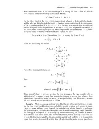
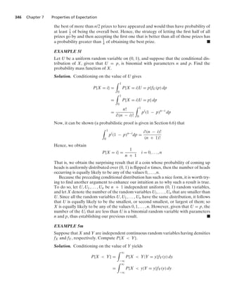
362. Section 7.5 Conditional Expectation 347
=
* q
−q
P{X y}fY(y} dy by independence
=
* q
−q
FX(y)fY(y) dy
where
FX(y) =
* y
−q
fX(x) dx .
EXAMPLE 5n
Suppose that X and Y are independent continuous random variables. Find the distri-
bution of X + Y.
Solution. By conditioning on the value of Y, we obtain
P{X + Y a} =
* q
−q
P{X + Y a|Y = y}fY(y) dy
=
* q
−q
P{X + y a|Y = y}fY(y) dy
=
* q
−q
P{X a − y}fY(y) dy
=
* q
−q
FX(a − y)fY(y) dy .
7.5.4 Conditional Variance
Just as we have defined the conditional expectation of X given the value of Y, we can
also define the conditional variance of X given that Y = y:
Var(X|Y) K E[(X − E[X|Y])2
|Y]
That is, Var(X|Y) is equal to the (conditional) expected square of the difference
between X and its (conditional) mean when the value of Y is given. In other words,
Var(X|Y) is exactly analogous to the usual definition of variance, but now all expec-
tations are conditional on the fact that Y is known.
There is a very useful relationship between Var(X), the unconditional variance of
X, and Var(X|Y), the conditional variance of X given Y, that can often be applied to
compute Var(X). To obtain this relationship, note first that, by the same reasoning
that yields Var(X) = E[X2] − (E[X])2, we have
Var(X|Y) = E[X2
|Y] − (E[X|Y])2
so
E[Var(X|Y)] = E[E[X2
|Y]] − E[(E[X|Y])2
]
= E[X2
] − E[(E[X|Y])2
] (5.9)

363. 348 Chapter 7 Properties of Expectation
Also, since E[E[X|Y]] = E[X], we have
Var(E[X|Y]) = E[(E[X|Y])2
] − (E[X])2
(5.10)
Hence, by adding Equations (5.9) and (5.10), we arrive at the following proposition.
Proposition 5.2. The conditional variance formula
Var(X) = E[Var(X|Y)] + Var(E[X|Y])
EXAMPLE 5o
Suppose that by any time t the number of people that have arrived at a train depot is
a Poisson random variable with mean λt. If the initial train arrives at the depot at a
time (independent of when the passengers arrive) that is uniformly distributed over
(0, T), what are the mean and variance of the number of passengers who enter the
train?
Solution. For each t Ú 0, let N(t) denote the number of arrivals by t, and let Y denote
the time at which the train arrives. The random variable of interest is then N(Y).
Conditioning on Y gives
E[N(Y)|Y = t] = E[N(t)|Y = t]
= E[N(t)] by the independence of Y and N(t)
= λt since N(t) is Poisson with mean λt
Hence,
E[N(Y)|Y] = λY
so taking expectations gives
E[N(Y)] = λE[Y] =
λT
2
To obtain Var(N(Y)), we use the conditional variance formula:
Var(N(Y)|Y = t) = Var(N(t)|Y = t)
= Var(N(t)) by independence
= λt
Thus,
Var(N(Y)|Y) = λY
E[N(Y)|Y] = λY
Hence, from the conditional variance formula,
Var(N(Y)) = E[λY] + Var(λY)
= λ
T
2
+ λ2 T2
12
where we have used the fact that Var(Y) = T2/12. .

364. Section 7.6 Conditional Expectation and Prediction 349
EXAMPLE 5p Variance of a sum of a random number of random variables
Let X1, X2, ... be a sequence of independent and identically distributed random vari-
ables, and let N be a nonnegative integer-valued random variable that is independent
of the sequence Xi, i Ú 1. To compute Var
N
i=1
Xi
, we condition on N:
E
⎡
⎣
N
i=1
Xi|N
⎤
⎦ = NE[X]
Var
⎛
⎝
N
i=1
Xi|N
⎞
⎠ = NVar(X)
The preceding result follows because, given N, N
i=1 Xi is just the sum of a fixed num-
ber of independent random variables, so its expectation and variance are just the
sums of the individual means and variances, respectively. Hence, from the conditional
variance formula,
Var
⎛
⎝
N
i=1
Xi
⎞
⎠ = E[N]Var(X) + (E[X])2
Var(N) .
7.6 CONDITIONAL EXPECTATION AND PREDICTION
Sometimes a situation arises in which the value of a random variable X is observed
and then, on the basis of the observed value, an attempt is made to predict the value
of a second random variable Y. Let g(X) denote the predictor; that is, if X is observed
to equal x, then g(x) is our prediction for the value of Y. Clearly, we would like to
choose g so that g(X) tends to be close to Y. One possible criterion for closeness is to
choose g so as to minimize E[(Y − g(X))2]. We now show that, under this criterion,
the best possible predictor of Y is g(X) = E[Y|X].
Proposition 6.1.
E[(Y − g(X))2
] Ú E[(Y − E[Y|X])2
]
Proof.
E[(Y − g(X))2
|X] = E[(Y − E[Y|X] + E[Y|X] − g(X))2
|X]
= E[(Y − E[Y|X])2
|X]
+ E[(E[Y|X] − g(X))2
|X]
+ 2E[(Y − E[Y|X])(E[Y|X] − g(X))|X] (6.1)
However, given X, E[Y|X] − g(X), being a function of X, can be treated as a
constant. Thus,
E[(Y − E[Y|X])(E[Y|X] − g(X))|X]
= (E[Y|X] − g(X))E[Y − E[Y|X]|X]
= (E[Y|X] − g(X))(E[Y|X] − E[Y|X])
= 0 (6.2)

365. 350 Chapter 7 Properties of Expectation
Hence, from Equations (6.1) and (6.2), we obtain
E[(Y − g(X))2
|X] Ú E[(Y − E[Y|X])2
|X]
and the desired result follows by taking expectations of both sides of the preceding
expression.
Remark. A second, more intuitive, although less rigorous, argument verifying
Proposition 6.1 is as follows. It is straightforward to verify that E[(Y − c)2] is mini-
mized at c = E[Y]. (See Theoretical Exercise 1.) Thus, if we want to predict the value
of Y when there are no data available to use, the best possible prediction, in the
sense of minimizing the mean square error, is to predict that Y will equal its mean.
However, if the value of the random variable X is observed to be x, then the predic-
tion problem remains exactly as in the previous (no-data) case, with the exception
that all probabilities and expectations are now conditional on the event that X = x.
Hence, the best prediction in this situation is to predict that Y will equal its condi-
tional expected value given that X = x, thus establishing Proposition 6.1. .
EXAMPLE 6a
Suppose that the son of a man of height x (in inches) attains a height that is normally
distributed with mean x + 1 and variance 4. What is the best prediction of the height
at full growth of the son of a man who is 6 feet tall?
Solution. Formally, this model can be written as
Y = X + 1 + e
where e is a normal random variable, independent of X, having mean 0 and variance
4. The X and Y, of course, represent the heights of the man and his son, respectively.
The best prediction E[Y|X = 72] is thus equal to
E[Y|X = 72] = E[X + 1 + e|X = 72]
= 73 + E[e|X = 72]
= 73 + E(e) by independence
= 73 .
EXAMPLE 6b
Suppose that if a signal value s is sent from location A, then the signal value received
at location B is normally distributed with parameters (s, 1). If S, the value of the signal
sent at A, is normally distributed with parameters (μ, σ2), what is the best estimate of
the signal sent if R, the value received at B, is equal to r?
Solution. Let us start by computing the conditional density of S given R. We have
fS|R(s|r) =
fS, R(s, r)
fR(r)
=
fS(s)fR|S(r|s)
fR(r)
= Ke−(s−μ)2/2σ2
e−(r−s)2/2

366. Section 7.6 Conditional Expectation and Prediction 351
where K does not depend on s. Now,
(s − μ)2
2σ2
+
(r − s)2
2
= s2
1
2σ2
+
1
2
−
μ
σ2
+ r
s + C1
=
1 + σ2
2σ2
⎡
⎣s2
− 2
μ + rσ2
1 + σ2
s
⎤
⎦ + C1
=
1 + σ2
2σ2
s −
(μ + rσ2)
1 + σ2
2
+ C2
where C1 and C2 do not depend on s. Hence,
fS|R(s|r) = C exp
⎧
⎪
⎪
⎪
⎪
⎪
⎪
⎨
⎪
⎪
⎪
⎪
⎪
⎪
⎩
−
s −
(μ + rσ2)
1 + σ2
2
2
σ2
1 + σ2
⎫
⎪
⎪
⎪
⎪
⎪
⎪
⎬
⎪
⎪
⎪
⎪
⎪
⎪
⎭
where C does not depend on s. Thus, we may conclude that the conditional distribu-
tion of S, the signal sent, given that r is received, is normal with mean and variance
now given by
E[S|R = r] =
μ + rσ2
1 + σ2
Var(S|R = r) =
σ2
1 + σ2
Consequently, from Proposition 6.1, given that the value received is r, the best esti-
mate, in the sense of minimizing the mean square error, for the signal sent is
E[S|R = r] =
1
1 + σ2
μ +
σ2
1 + σ2
r
Writing the conditional mean as we did previously is informative, for it shows that it
equals a weighted average of μ, the a priori expected value of the signal, and r, the
value received. The relative weights given to μ and r are in the same proportion to
each other as 1 (the conditional variance of the received signal when s is sent) is to σ2
(the variance of the signal to be sent). .
EXAMPLE 6c
In digital signal processing, raw continuous analog data X must be quantized, or dis-
cretized, in order to obtain a digital representation. In order to quantize the raw
data X, an increasing set of numbers ai, i = 0, ;1, ;2, ..., such that lim
i→+q
ai = q and
lim
i→−q
ai = −q is fixed, and the raw data are then quantized according to the interval
(ai, ai+1] in which X lies. Let us denote by yi the discretized value when X ∈ (ai, ai+1],
and let Y denote the observed discretized value—that is,
Y = yi if ai X … ai+1

367. 352 Chapter 7 Properties of Expectation
The distribution of Y is given by
P{Y = yi} = FX(ai+1) − FX(ai)
Suppose now that we want to choose the values yi, i = 0, ;1, ;2, ... so as to mini-
mize E[(X − Y)2], the expected mean square difference between the raw data and
their quantized version.
(a) Find the optimal values yi, i = 0, ;1, ....
For the optimal quantizer Y, show that
(b) E[Y] = E[X], so the mean square error quantizer preserves the input mean;
(c) Var(Y) = Var(X) − E[(X − Y)2].
Solution. (a) For any quantizer Y, upon conditioning on the value of Y, we obtain
E[(X − Y)2
] =
i
E[(X − yi)2
|ai X … ai+1]P{ai X … ai+1}
Now, if we let
I = i if ai X … ai+1
then
E[(X − yi)2
|ai X … ai+1] = E[(X − yi)2
|I = i]
and by Proposition 6.1, this quantity is minimized when
yi = E[X|I = i]
= E[X|ai X … ai+1]
=
* ai+1
ai
xfX(x) dx
FX(ai+1) − FX(ai)
Now, since the optimal quantizer is given by Y = E[X|I], it follows that
(b) E[Y] = E[X]
(c)
Var(X) = E[Var(X|I)] + Var(E[X|I])
= E[E[(X − Y)2
|I]] + Var(Y)
= E[(X − Y)2
] + Var(Y) .
It sometimes happens that the joint probability distribution of X and Y is not
completely known; or if it is known, it is such that the calculation of E[Y|X = x]
is mathematically intractable. If, however, the means and variances of X and Y and
the correlation of X and Y are known, then we can at least determine the best linear
predictor of Y with respect to X.
To obtain the best linear predictor of Y with respect to X, we need to choose a and
b so as to minimize E[(Y − (a + bX))2]. Now,
E[(Y − (a + bX))2
] = E[Y2
− 2aY − 2bXY + a2
+ 2abX + b2
X2
]
= E[Y2
] − 2aE[Y] − 2bE[XY] + a2
+ 2abE[X] + b2
E[X2
]

368. Section 7.6 Conditional Expectation and Prediction 353
Taking partial derivatives, we obtain
∂
∂a
E[(Y − a − bX)2
] = −2E[Y] + 2a + 2bE[X]
∂
∂b
E[(Y − a − bX)2
] = −2E[XY] + 2aE[X] + 2bE[X2
]
(6.3)
Setting Equations (6.3) to 0 and solving for a and b yields the solutions
b =
E[XY] − E[X]E[Y]
E[X2] − (E[X])2
=
Cov(X, Y)
σ2
x
= ρ
σy
σx
a = E[Y] − bE[X] = E[Y] −
ρσyE[X]
σx
(6.4)
where ρ = Correlation(X, Y), σ2
y = Var(Y), and σ2
x = Var(X). It is easy to ver-
ify that the values of a and b from Equation (6.4) minimize E[(Y − a − bX)2];
thus, the best (in the sense of mean square error) linear predictor Y with respect
to X is
μy +
ρσy
σx
(X − μx)
where μy = E[Y] and μx = E[X].
The mean square error of this predictor is given by
E
Y − μy − ρ
σy
σx
(X − μx)
2
= E
4
(Y − μy)2
5
+ ρ2
σ2
y
σ2
x
E
4
(X − μx)2
5
− 2ρ
σy
σx
E
2
(Y − μy)(X − μx)
3
= σ2
y + ρ2
σ2
y − 2ρ2
σ2
y
= σ2
y (1 − ρ2
) (6.5)
We note from Equation (6.5) that if ρ is near +1 or −1, then the mean square error
of the best linear predictor is near zero. .
EXAMPLE 6d
An example in which the conditional expectation of Y given X is linear in X, and
hence in which the best linear predictor of Y with respect to X is the best overall
predictor, is when X and Y have a bivariate normal distribution. For, as shown in
Example 5c of Chapter 6, in that case,
E[Y|X = x] = μy + ρ
σy
σx
(x − μx) .

369. 354 Chapter 7 Properties of Expectation
7.7 MOMENT GENERATING FUNCTIONS
The moment generating function M(t) of the random variable X is defined for all real
values of t by
M(t) = E[etX
]
=
⎧
⎪
⎪
⎪
⎨
⎪
⎪
⎪
⎩
x
etx
p(x) if X is discrete with mass function p(x)
* q
−q
etx
f(x) dx if X is continuous with density f(x)
We call M(t) the moment generating function because all of the moments of X can be
obtained by successively differentiating M(t) and then evaluating the result at t = 0.
For example,
M
(t) =
d
dt
E[etX
]
= E
d
dt
(etX
)
(7.1)
= E[XetX
]
where we have assumed that the interchange of the differentiation and expectation
operators is legitimate. That is, we have assumed that
d
dt
⎡
⎣
x
etx
p(x)
⎤
⎦ =
x
d
dt
[etx
p(x)]
in the discrete case and
d
dt
*
etx
f(x) dx
=
*
d
dt
[etx
f(x)] dx
in the continuous case. This assumption can almost always be justified and, indeed, is
valid for all of the distributions considered in this book. Hence, from Equation (7.1),
evaluated at t = 0, we obtain
M
(0) = E[X]
Similarly,
M
(t) =
d
dt
M
(t)
=
d
dt
E[XetX
]
= E
d
dt
(XetX
)
= E[X2
etX
]
Thus,
M
(0) = E[X2
]

370. Section 7.7 Moment Generating Functions 355
In general, the nth derivative of M(t) is given by
Mn
(t) = E[Xn
etX
] n Ú 1
implying that
Mn
(0) = E[Xn
] n Ú 1
We now compute M(t) for some common distributions.
EXAMPLE 7a Binomial distribution with parameters n and p
If X is a binomial random variable with parameters n and p, then
M(t) = E[etX
]
=
n
k=0
etk
n
k
pk
(1 − p)n−k
=
n
k=0
n
k
(pet
)k
(1 − p)n−k
= (pet
+ 1 − p)n
where the last equality follows from the binomial theorem. Differentiation yields
M
(t) = n(pet
+ 1 − p)n−1
pet
Thus,
E[X] = M
(0) = np
Differentiating a second time yields
M
(t) = n(n − 1)(pet
+ 1 − p)n−2
(pet
)2
+ n(pet
+ 1 − p)n−1
pet
so
E[X2
] = M
(0) = n(n − 1)p2
+ np
The variance of X is given by
Var(X) = E[X2
] − (E[X])2
= n(n − 1)p2
+ np − n2
p2
= np(1 − p)
verifying the result obtained previously. .
EXAMPLE 7b Poisson distribution with mean λ
If X is a Poisson random variable with parameter λ, then
M(t) = E[etX
]
=
q
n=0
etne−λλn
n!
= e−λ
q
n=0
(λet)n
n!

371. 356 Chapter 7 Properties of Expectation
= e−λ
eλet
= exp{λ(et
− 1)}
Differentiation yields
M
(t) = λet
exp{λ(et
− 1)}
M
(t) = (λet
)2
exp{λ(et
− 1)} + λet
exp{λ(et
− 1)}
Thus,
E[X] = M
(0) = λ
E[X2
] = M
(0) = λ2
+ λ
Var(X) = E[X2
] − (E[X])2
= λ
Hence, both the mean and the variance of the Poisson random variable equal λ. .
EXAMPLE 7c Exponential distribution with parameter λ
M(t) = E[etX
]
=
* q
0
etx
λe−λx
dx
= λ
* q
0
e−(λ−t)x
dx
=
λ
λ − t
for t λ
We note from this derivation that, for the exponential distribution, M(t) is defined
only for values of t less than λ. Differentiation of M(t) yields
M
(t) =
λ
(λ − t)2
M
(t) =
2λ
(λ − t)3
Hence,
E[X] = M
(0) =
1
λ
E[X2
] = M
(0) =
2
λ2
The variance of X is given by
Var(X) = E[X2
] − (E[X])2
=
1
λ2
.
EXAMPLE 7d Normal distribution
We first compute the moment generating function of a unit normal random variable
with parameters 0 and 1. Letting Z be such a random variable, we have
MZ(t) = E[etZ
]
=
1
√
2π
* q
−q
etx
e−x2/2
dx

372. Section 7.7 Moment Generating Functions 357
=
1
√
2π
* q
−q
exp
0
−
(x2 − 2tx)
2
7
dx
=
1
√
2π
* q
−q
exp
0
−
(x − t)2
2
+
t2
2
7
dx
= et2/2 1
√
2π
* q
−q
e−(x−t)2/2
dx
= et2/2
Hence, the moment generating function of the unit normal random variable Z is given
by MZ(t) = et2/2. To obtain the moment generating function of an arbitrary normal
random variable, we recall (see Section 5.4) that X = μ + σZ will have a normal
distribution with parameters μ and σ2 whenever Z is a unit normal random variable.
Hence, the moment generating function of such a random variable is given by
MX(t) = E[etX
]
= E[et(μ+σZ)
]
= E[etμ
etσZ
]
= etμ
E[etσZ
]
= etμ
MZ(tσ)
= etμ
e(tσ)2/2
= exp
0
σ2t2
2
+ μt
7
By differentiating, we obtain
M
X(t) = (μ + tσ2
) exp
0
σ2t2
2
+ μt
7
M
X(t) = (μ + tσ2
)2
exp
0
σ2t2
2
+ μt
7
+ σ2
exp
0
σ2t2
2
+ μt
7
Thus,
E[X] = M
(0) = μ
E[X2
] = M
(0) = μ2
+ σ2
implying that
Var(X) = E[X2
] − E([X])2
= σ2
.
Tables 7.1 and 7.2 give the moment generating functions for some common dis-
crete and continuous distributions.
An important property of moment generating functions is that the moment gen-
erating function of the sum of independent random variables equals the product of
the individual moment generating functions. To prove this, suppose that X and Y are

373. 358 Chapter 7 Properties of Expectation
TABLE 7.1: DISCRETE PROBABILITY DISTRIBUTION
Moment
Probability mass generating
function, p(x) function, M(t) Mean Variance
Binomial with
parameters n, p;
0 … p … 1
n
x
px(1 − p)n−x (pet + 1 − p)n np np(1 − p)
x = 0, 1, ... , n
Poisson with
parameter λ 0
e−λ λx
x!
exp{λ(et − 1)} λ λ
x = 0, 1, 2, ...
Geometric with
parameter
0 … p … 1
p(1 − p)x−1 pet
1 − (1 − p)et
1
p
1 − p
p2
x = 1, 2, ...
Negative
binomial with
parameters r, p;
0 … p … 1
n − 1
r − 1
pr(1 − p)n−r
pet
1 − (1 − p)et
r
r
p
r(1 − p)
p2
n = r, r + 1, ...
independent and have moment generating functions MX(t) and MY(t), respectively.
Then MX+Y(t), the moment generating function of X + Y, is given by
MX+Y(t) = E[et(X+Y)
]
= E[etX
etY
]
= E[etX
]E[etY
]
= MX(t)MY(t)
where the next-to-last equality follows from Proposition 4.1, since X and Y are inde-
pendent.
Another important result is that the moment generating function uniquely deter-
mines the distribution. That is, if MX(t) exists and is finite in some region about t = 0,
then the distribution of X is uniquely determined. For instance, if
MX(t) =
1
2
10
(et
+ 1)10
,
then it follows from Table 7.1 that X is a binomial random variable with parameters
10 and 1
2 .
EXAMPLE 7e
Suppose that the moment generating function of a random variable X is given by
M(t) = e3(et−1). What is P{X = 0}?

374. Section
7.7
Moment
Generating
Functions
359
TABLE 7.2: CONTINUOUS PROBABILITY DISTRIBUTION
Moment
generating
Probability mass function, f(x) function, M(t) Mean Variance
Uniform over (a, b) f(x) =
⎧
⎪
⎨
⎪
⎩
1
b − a
a x b
0 otherwise
etb − eta
t(b − a)
a + b
2
(b − a)2
12
Exponential with
parameter λ 0
f(x) =
0
λe−λx x Ú 0
0 x 0
λ
λ − t
1
λ
1
λ2
Gamma with parameters
(s, λ), λ 0
f(x) =
⎧
⎪
⎪
⎨
⎪
⎪
⎩
λe−λx(λx)s−1
(s)
x Ú 0
0 x 0
λ
λ − t
s
s
λ
s
λ2
Normal with parameters
(μ, σ2)
f(x) =
1
√
2πσ
e−(x−μ)2/2σ2
− q x q exp
0
μt +
σ2t2
2
7
μ σ2

375. 360 Chapter 7 Properties of Expectation
Solution. We see from Table 7.1 that M(t) = e3(et−1) is the moment generating func-
tion of a Poisson random variable with mean 3. Hence, by the one-to-one correspon-
dence between moment generating functions and distribution functions, it follows
that X must be a Poisson random variable with mean 3. Thus, P{X = 0} = e−3. .
EXAMPLE 7f Sums of independent binomial random variables
If X and Y are independent binomial random variables with parameters (n, p) and
(m, p), respectively, what is the distribution of X + Y?
Solution. The moment generating function of X + Y is given by
MX+Y(t) = MX(t)MY(t) = (pet
+ 1 − p)n
(pet
+ 1 − p)m
= (pet
+ 1 − p)m+n
However, (pet + 1 − p)m+n is the moment generating function of a binomial ran-
dom variable having parameters m + n and p. Thus, this must be the distribution
of X + Y. .
EXAMPLE 7g Sums of independent Poisson random variables
Calculate the distribution of X + Y when X and Y are independent Poisson random
variables with means respective λ1 and λ2.
Solution.
MX+Y(t) = MX(t)MY(t)
= exp{λ1(et
− 1)} exp{λ2(et
− 1)}
= exp{(λ1 + λ2)(et
− 1)}
Hence, X + Y is Poisson distributed with mean λ1 + λ2, verifying the result given
in Example 3e of Chapter 6. .
EXAMPLE 7h Sums of independent normal random variables
Show that if X and Y are independent normal random variables with respective
parameters (μ1, σ2
1 ) and (μ2, σ2
2 ), then X + Y is normal with mean μ1 + μ2 and
variance σ2
1 + σ2
2 .
Solution.
MX+Y(t) = MX(t)MY(t)
= exp
0
σ2
1 t2
2
+ μ1t
7
exp
0
σ2
2 t2
2
+ μ2t
7
= exp
0
(σ2
1 + σ2
2 )t2
2
+ (μ1 + μ2)t
7
which is the moment generating function of a normal random variable with mean
μ1 + μ2 and variance σ2
1 + σ2
2 . The desired result then follows because the moment
generating function uniquely determines the distribution. .

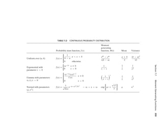
376. Section 7.7 Moment Generating Functions 361
EXAMPLE 7i
Compute the moment generating function of a chi-squared random variable with n
degrees of freedom.
Solution. We can represent such a random variable as
Z2
1 + · · · + Z2
n
where Z1, ... , Zn are independent standard normal random variables. Let M(t) be its
moment generating function. Then, by the preceding,
M(t) = (E[etZ2
])n
where Z is a standard normal random variable. Now,
E[etZ2
] =
1
√
2π
* q
−q
etx2
e−x2/2
dx
=
1
√
2π
* q
−q
e−x2/2σ2
dx where σ2
= (1 − 2t)−1
= σ
= (1 − 2t)−1/2
where the next-to-last equality uses the fact that the normal density with mean 0 and
variance σ2 integrates to 1. Therefore,
M(t) = (1 − 2t)−n/2
.
EXAMPLE 7j Moment generating function of the sum of a random number of
random variables
Let X1, X2, ... be a sequence of independent and identically distributed random vari-
ables, and let N be a nonnegative, integer-valued random variable that is independent
of the sequence X, i Ú 1. We want to compute the moment generating function of
Y =
N
i=1
Xi
(In Example 5d, Y was interpreted as the amount of money spent in a store on a
given day when both the amount spent by a customer and the number of customers
are random variables.)
To compute the moment generating function of Y, we first condition on N as
follows:
E
⎡
⎢
⎢
⎣exp
⎧
⎨
⎩
t
N
1
Xi
⎫
⎬
⎭
6
6
6
6
6
6
6
N = n
⎤
⎥
⎥
⎦ = E
⎡
⎢
⎢
⎣exp
⎧
⎨
⎩
t
n
1
Xi
⎫
⎬
⎭
6
6
6
6
6
6
6
N = n
⎤
⎥
⎥
⎦
= E
⎡
⎢
⎣exp
⎧
⎨
⎩
t
n
1
Xi
⎫
⎬
⎭
⎤
⎥
⎦
= [MX(t)]n

377. 362 Chapter 7 Properties of Expectation
where
MX(t) = E[etXi ]
Hence,
E[etY
|N] = (MX(t))N
Thus,
MY(t) = E[(MX(t))N
]
The moments of Y can now be obtained upon differentiation, as follows:
M
Y(t) = E[N(MX(t))N−1
M
X(t)]
So
E[Y] = M
Y(0)
= E[N(MX(0))N−1
M
X(0)]
= E[NEX] (7.2)
= E[N]E[X]
verifying the result of Example 5d. (In this last set of equalities, we have used the fact
that MX(0) = E[e0X] = 1.)
Also,
M
Y(t) = E[N(N − 1)(MX(t))N−2
(M
X(t))2
+ N(MX(t))N−1
M
X(t)]
so
E[Y2
] = M
Y(0)
= E[N(N − 1)(E[X])2
+ NE[X2
]]
= (E[X])2
(E[N2
] − E[N]) + E[N]E[X2
] (7.3)
= E[N](E[X2
] − (E[X])2
) + (E[X])2
E[N2
]
= E[N]Var(X) + (E[X])2
E[N2
]
Hence, from Equations (7.2) and (7.3), we have
Var(Y) = E[N]Var(X) + (E[X])2
(E[N2
] − (E[N])2
)
= E[N]Var(X) + (E[X])2
Var(N) .
EXAMPLE 7k
Let Y denote a uniform random variable on (0, 1), and suppose that, conditional on
Y = p, the random variable X has a binomial distribution with parameters n and p.
In Example 5k, we showed that X is equally likely to take on any of the values
0, 1, ... , n. Establish this result by using moment generating functions.
Solution. To compute the moment generating function of X, start by conditioning
on the value of Y. Using the formula for the binomial moment generating function
gives
E[etX
|Y = p] = (pet
+ 1 − p)n

378. Section 7.7 Moment Generating Functions 363
Now, Y is uniform on (0, 1), so, upon taking expectations, we obtain
E[etX
] =
* 1
0
(pet
+ 1 − p)n
dp
=
1
et − 1
* et
1
yn
dy (by the substitution y = pet
+ 1 − p)
=
1
n + 1
et(n+1) − 1
et − 1
=
1
n + 1
(1 + et
+ e2t
+ · · · + ent
)
Because the preceding is the moment generating function of a random variable that
is equally likely to be any of the values 0, 1, ... , n, the desired result follows from the
fact that the moment generating function of a random variable uniquely determines
its distribution. .
7.7.1 Joint Moment Generating Functions
It is also possible to define the joint moment generating function of two or more
random variables. This is done as follows: For any n random variables X1, ... , Xn,
the joint moment generating function, M(t1, ... , tn), is defined, for all real values of
t1, ... , tn, by
M(t1, ... , tn) = E[et1X1+ · · · +tnXn ]
The individual moment generating functions can be obtained from M(t1, ... , tn) by
letting all but one of the tj’s be 0. That is,
MXi (t) = E[etXi ] = M(0, ... , 0, t, 0, ... , 0)
where the t is in the ith place.
It can be proven (although the proof is too advanced for this text) that the joint
moment generating function M(t1, ... , tn) uniquely determines the joint distribution
of X1, ... , Xn. This result can then be used to prove that the n random variables
X1, ... , Xn are independent if and only if
M(t1, ... , tn) = MX1
(t1) · · · MXn (tn) (7.4)
For the proof in one direction, if the n random variables are independent, then
M(t1, ... , tn) = E[e(t1X1+ · · · +tnXn)
]
= E[et1X1 · · · etnXn ]
= E[et1X1 ] · · · E[etnXn ] by independence
= MX1
(t1) · · · MXn (tn)
For the proof in the other direction, if Equation (7.4) is satisfied, then the joint
moment generating function M(t1, ... , tn) is the same as the joint moment generating
function of n independent random variables, the ith of which has the same distri-
bution as Xi. As the joint moment generating function uniquely determines the joint
distribution, this must be the joint distribution; hence, the random variables are
independent.

379. 364 Chapter 7 Properties of Expectation
EXAMPLE 7l
Let X and Y be independent normal random variables, each with mean μ and vari-
ance σ2. In Example 7a of Chapter 6, we showed that X + Y and X − Y are inde-
pendent. Let us now establish this result by computing their joint moment generating
function:
E[et(X+Y)+s(X−Y)
] = E[e(t+s)X+(t−s)Y
]
= E[e(t+s)X
]E[e(t−s)Y
]
= eμ(t+s)+σ2(t+s)2/2
eμ(t−s)+σ2(t−s)2/2
= e2μt+σ2t2
eσ2s2
But we recognize the preceding as the joint moment generating function of the sum
of a normal random variable with mean 2μ and variance 2σ2 and an independent
normal random variable with mean 0 and variance 2σ2. Because the joint moment
generating function uniquely determines the joint distribution, it follows that X + Y
and X − Y are independent normal random variables. .
In the next example, we use the joint moment generating function to verify a result
that was established in Example 2b of Chapter 6.
EXAMPLE 7m
Suppose that the number of events that occur is a Poisson random variable with
mean λ and that each event is independently counted with probability p. Show that
the number of counted events and the number of uncounted events are independent
Poisson random variables with respective means λp and λ(1 − p).
Solution. Let X denote the total number of events, and let Xc denote the number
of them that are counted. To compute the joint moment generating function of Xc,
the number of events that are counted, and X − Xc, the number that are uncounted,
start by conditioning on X to obtain
E[esXc+t(X−Xc)
|X = n] = etn
E[e(s−t)Xc |X = n]
= etn
(pes−t
+ 1 − p)n
= (pes
+ (1 − p)et
)n
which follows because, conditional on X = n, Xc is a binomial random variable with
parameters n and p. Hence,
E[esXc+t(X−Xc)
|X] = (pes
+ (1 − p)et
)X
Taking expectations of both sides of this equation yields
E[esXc+t(X−Xc)
] = E[(pes
+ (1 − p)et
)X
]
Now, since X is Poisson with mean λ, it follows that E[etX] = eλ(et−1). Therefore, for
any positive value a we see (by letting a = et) that E[aX] = eλ(a−1). Thus
E[esXc+t(X−Xc)
] = eλ(pes+(1−p)et−1)
= eλp(es−1 )
eλ(1−p)(et−1)

380. Section 7.8 Additional Properties of Normal Random Variables 365
As the preceding is the joint moment generating function of independent Poisson
random variables with respective means λp and λ(1 − p), the result is proven. .
7.8 ADDITIONAL PROPERTIES OF NORMAL RANDOM VARIABLES
7.8.1 The Multivariate Normal Distribution
Let Z1, ... , Zn be a set of n independent unit normal random variables. If, for some
constants aij, 1 … i … m, 1 … j … n, and μi, 1 … i … m,
X1 = a11Z1 + · · · + a1nZn + μ1
X2 = a21Z1 + · · · + a2nZn + μ2
.
.
.
Xi = ai1Z1 + · · · + ainZn + μi
.
.
.
Xm = am1Z1 + · · · + amnZn + μm
then the random variables X1, ... , Xm are said to have a multivariate normal distri-
bution.
From the fact that the sum of independent normal random variables is itself a
normal random variable, it follows that each Xi is a normal random variable with
mean and variance given, respectively, by
E[Xi] = μi
Var(Xi) =
n
j=1
a2
ij
Let us now consider
M(t1, ... , tm) = E[exp{t1X1 + · · · + tmXm}]
the joint moment generating function of X1, ... , Xm. The first thing to note is that
since
m
i=1
tiXi is itself a linear combination of the independent normal random vari-
ables Z1, ... , Zn, it is also normally distributed. Its mean and variance are
E
⎡
⎣
m
i=1
tiXi
⎤
⎦ =
m
i=1
tiμi
and
Var
⎛
⎝
m
i=1
tiXi
⎞
⎠ = Cov
⎛
⎜
⎝
m
i=1
tiXi,
m
j=1
tjXj
⎞
⎟
⎠
=
m
i=1
m
j=1
titjCov(Xi, Xj)

381. 366 Chapter 7 Properties of Expectation
Now, if Y is a normal random variable with mean μ and variance σ2, then
E[eY
] = MY(t)|t=1 = eμ+σ2/2
Thus,
M(t1, ... , tm) = exp
⎧
⎪
⎨
⎪
⎩
m
i=1
tiμi +
1
2
m
i=1
m
j=1
titjCov(Xi, Xj)
⎫
⎪
⎬
⎪
⎭
which shows that the joint distribution of X1, ... , Xm is completely determined from
a knowledge of the values of E[Xi] and Cov(Xi, Xj), i, j = 1, ... , m.
It can be shown that when m = 2, the multivariate normal distribution reduces to
the bivariate normal.
EXAMPLE 8a
Find P(X Y) for bivariate normal random variables X and Y having parameters
μx = E[X], μy = E[Y], σ2
x = Var(X), σ2
y = Var(Y), ρ = Corr(X, Y)
Solution. Because X − Y is normal with mean
E[X − Y] = μx − μy
and variance
Var(X − Y) = Var(X) + Var(−Y) + 2Cov(X, −Y)
= σ2
x + σ2
y − 2ρσxσy
we obtain
P{X Y} = P{X − Y 0}
= P
⎧
⎪
⎨
⎪
⎩
X − Y − (μx − μy)
8
σ2
x + σ2
y − 2ρσxσy
−(μx − μy)
8
σ2
x + σ2
y − 2ρσxσy
⎫
⎪
⎬
⎪
⎭
=
μy − μx
8
σ2
x + σ2
y − 2ρσxσy
.
EXAMPLE 8b
Suppose that the conditional distribution of X, given that = θ, is normal with
mean θ and variance 1. Moreover, suppose that itself is a normal random variable
with mean μ and variance σ2. Find the conditional distribution of given that X = x.
Solution. Rather than using and then simplifying Bayes’s formula, we will solve this
problem by first showing that X, has a bivariate normal distribution. To do so, note
that the joint density function of X, can be written as
fX,(x, θ) = fX|(x|θ)f(θ)
where fX|(x|θ) is a normal density with mean θ and variance 1. However, if we let Z
be a standard normal random variable that is independent of , then the conditional
distribution of Z + , given that = θ, is also normal with mean θ and variance 1.

382. Section 7.8 Additional Properties of Normal Random Variables 367
Consequently, the joint density of Z + , is the same as that of X, . Because the
former joint density is clearly bivariate normal (since Z + and are both linear
combinations of the independent normal random variables Z and ), it follows that
X, has a bivariate normal distribution. Now,
E[X] = E[Z + ] = μ
Var(X) = Var(Z + ) = 1 + σ2
and
ρ = Corr(X, )
= Corr(Z + , )
=
Cov(Z + , )
√
Var(Z + )Var()
=
σ
.
1 + σ2
Because X, has a bivariate normal distribution, the conditional distribution of ,
given that X = x, is normal with mean
E[|X = x] = E[] + ρ
?
Var()
Var(X)
(x − E[X])
= μ +
σ2
1 + σ2
(x − μ)
and variance
Var(|X = x) = Var()(1 − ρ2
)
=
σ2
1 + σ2
.
7.8.2 The Joint Distribution of the Sample Mean and Sample Variance
Let X1, ... , Xn be independent normal random variables, each with mean μ and vari-
ance σ2. Let X =
n
i=1
Xi/n denote their sample mean. Since the sum of independent
normal random variables is also a normal random variable, it follows that X is a nor-
mal random variable with (from Examples 2c and 4a) expected value μ and variance
σ2/n.
Now, recall from Example 4e that
Cov(X, Xi − X) = 0, i = 1, ... , n (8.1)
Also, note that since X, X1 − X, X2 − X, ... , Xn − X are all linear combinations
of the independent standard normals (Xi − μ)/σ, i = 1, ... , n, it follows that X, Xi −
X, i = 1, ... , n has a joint distribution that is multivariate normal. If we let Y be
a normal random variable, with mean μ and variance σ2/n, that is independent of
the Xi, i = 1, ... , n, then Y, Xi − X, i = 1, ... , n also has a multivariate normal dis-
tribution and, indeed, because of Equation (8.1), has the same expected values and
covariances as the random variables X, Xi − X, i = 1, ... , n. But since a multivariate
normal distribution is determined completely by its expected values and covariances,

383. 368 Chapter 7 Properties of Expectation
it follows that Y, Xi − X, i = 1, ... , n and X, Xi − X, i = 1, ... , n have the same
joint distribution, thus showing that X is independent of the sequence of deviations
Xi − X, i = 1, ... , n.
Since X is independent of the sequence of deviations Xi − X, i = 1, ... , n, it is also
independent of the sample variance S2 K
n
i=1
(Xi − X)2/(n − 1).
Since we already know that X is normal with mean μ and variance σ2/n, it remains
only to determine the distribution of S2. To accomplish this, recall, from Example 4a,
the algebraic identity
(n − 1)S2
=
n
i=1
(Xi − X)2
=
n
i=1
(Xi − μ)2
− n(X − μ)2
Upon dividing the preceding equation by σ2, we obtain
(n − 1)S2
σ2
+
X − μ
σ/
√
n
2
=
n
i=1
Xi − μ
σ
2
(8.2)
Now,
n
i=1
Xi − μ
σ
2
is the sum of the squares of n independent standard normal random variables and so
is a chi-squared random variable with n degrees of freedom. Hence, from Example 7i,
its moment generating function is (1 − 2t)−n/2. Also, because
X − μ
σ/
√
n
2
is the square of a standard normal variable, it is a chi-squared random variable with
1 degree of freedom, and so has moment generating function (1 − 2t)−1/2. Now, we
have seen previously that the two random variables on the left side of Equation (8.2)
are independent. Hence, as the moment generating function of the sum of indepen-
dent random variables is equal to the product of their individual moment generating
functions, we have
E[et(n−1)S2/σ2
](1 − 2t)−1/2
= (1 − 2t)−n/2
or
E[et(n−1)S2/σ2
] = (1 − 2t)−(n−1)/2
But as (1 − 2t)−(n−1)/2 is the moment generating function of a chi-squared random
variable with n − 1 degrees of freedom, we can conclude, since the moment gener-
ating function uniquely determines the distribution of the random variable, it follows
that that is the distribution of (n − 1)S2/σ2.
Summing up, we have shown the following.

384. Section 7.9 General Definition of Expectation 369
Proposition 8.1. If X1, ... , Xn are independent and identically distributed normal
random variables with mean μ and variance σ2, then the sample mean X and the
sample variance S2 are independent. X is a normal random variable with mean μ and
variance σ2/n; (n − 1)S2/σ2 is a chi-squared random variable with n − 1 degrees of
freedom.
7.9 GENERAL DEFINITION OF EXPECTATION
Up to this point, we have defined expectations only for discrete and continuous ran-
dom variables. However, there also exist random variables that are neither discrete
nor continuous, and they, too, may possess an expectation. As an example of such a
random variable, let X be a Bernoulli random variable with parameter p = 1
2, and let
Y be a uniformly distributed random variable over the interval [0, 1]. Furthermore,
suppose that X and Y are independent, and define the new random variable W by
W =
%
X if X = 1
Y if X Z 1
Clearly, W is neither a discrete (since its set of possible values, [0, 1], is uncountable)
nor a continuous (since P{W = 1} = 1
2 ) random variable.
In order to define the expectation of an arbitrary random variable, we require the
notion of a Stieltjes integral. Before defining this integral, let us recall that, for any
function g,
- b
a g(x) dx is defined by
* b
a
g(x) dx = lim
n
i=1
g(xi)(xi − xi−1)
where the limit is taken over all a = x0 x1 x2 · · · xn = b as n→q and where
max
i=1,...,n
(xi − xi−1)→0.
For any distribution function F, we define the Stieltjes integral of the nonnegative
function g over the interval [a, b] by
* b
a
g(x) dF(x) = lim
n
i=1
g(xi)[F(xi) − F(xi−1)]
where, as before, the limit is taken over all a = x0 x1 · · · xn = b as n→q and
where max
i=1,...,n
(xi − xi−1)→0. Further, we define the Stieltjes integral over the whole
real line by
* q
−q
g(x) dF(x) = lim
a→ − q
b→ + q
* b
a
g(x) dF(x)
Finally, if g is not a nonnegative function, we define g+ and g− by
g+
(x) =
%
g(x) if g(x) Ú 0
0 if g(x) 0
g−
(x) =
%
0 if g(x) Ú 0
−g(x) if g(x) 0

385. 370 Chapter 7 Properties of Expectation
Because g(x) = g+(x) − g−(x) and g+ and g− are both nonnegative functions, it is
natural to define
* q
−q
g(x) dF(x) =
* q
−q
g+
(x) dF(x) −
* q
−q
g−
(x) dF(x)
and we say that
- q
−q g(x) dF(x) exists as long as
- q
−q g+(x) dF(x) and
- q
−q g−(x) dF(x)
are not both equal to +q.
If X is an arbitrary random variable having cumulative distribution F, we define
the expected value of X by
E[X] =
* q
−q
x dF(x) (9.1)
It can be shown that if X is a discrete random variable with mass function p(x), then
* q
−q
xdF(x) =
x:p(x)0
xp(x)
whereas if X is a continuous random variable with density function f(x), then
* q
−q
xdF(x) =
* q
−q
xf(x) dx
The reader should note that Equation (9.1) yields an intuitive definition of E[X];
consider the approximating sum
n
i=1
xi[F(xi) − F(xi−1)]
of E[X]. Because F(xi) − F(xi−1) is just the probability that X will be in the interval
(xi−1, xi], the approximating sum multiplies the approximate value of X when it is in
the interval (xi−1, xi] by the probability that it will be in that interval and then sums
over all the intervals. Clearly, as these intervals get smaller and smaller in length, we
obtain the “expected value” of X.
Stieltjes integrals are mainly of theoretical interest because they yield a compact
way of defining and dealing with the properties of expectation. For instance, the use
of Stieltjes integrals avoids the necessity of having to give separate statements and
proofs of theorems for the continuous and the discrete cases. However, their prop-
erties are very much the same as those of ordinary integrals, and all of the proofs
presented in this chapter can easily be translated into proofs in the general case.
SUMMARY
If X and Y have a joint probability mass function p(x, y), then
E[g(X, Y)] =
y
x
g(x, y)p(x, y)
whereas if they have a joint density function f(x, y), then
E[g(X, Y)] =
* q
−q
* q
−q
g(x, y)f(x, y) dx dy
A consequence of the preceding equations is that
E[X + Y] = E[X] + E[Y]

386. Summary 371
which generalizes to
E
⎡
⎣
n
i=1
Xi
⎤
⎦ =
n
i=1
E[Xi]
The covariance between random variables X and Y is given by
Cov(X, Y) = E[(X − E[X])(Y − E[Y])] = E[XY] − E[X]E[Y]
A useful identity is
Cov
⎛
⎜
⎝
n
i=1
Xi,
m
j=1
Yj
⎞
⎟
⎠ =
n
i=1
m
j=1
Cov(Xi, Yj)
When n = m and Yi = Xi, i = 1, ... , n, the preceding formula gives
Var
⎛
⎝
n
i=1
Xi
⎞
⎠ =
n
i=1
Var(Xi) + 2
ij
Cov(Xi, Yj)
The correlation between X and Y, denoted by ρ(X, Y), is defined by
ρ(X, Y) =
Cov(X, Y)
√
Var(X)Var(Y)
If X and Y are jointly discrete random variables, then the conditional expected value
of X, given that Y = y, is defined by
E[X|Y = y] =
x
xP{X = x|Y = y]
If X and Y are jointly continuous random variables, then
E[X|Y = y] =
* q
−q
xfX|Y(x|y)
where
fX|Y(x|y) =
f(x, y)
fY(y)
is the conditional probability density of X given that Y = y. Conditional expecta-
tions, which are similar to ordinary expectations except that all probabilities are now
computed conditional on the event that Y = y, satisfy all the properties of ordinary
expectations.
Let E[X|Y] denote that function of Y whose value at Y = y is E[X|Y = y]. A very
useful identity is
E[X] = E[E[X|Y]]
In the case of discrete random variables, this equation reduces to the identity
E[X] =
y
E[X|Y = y]P{Y = y}
and, in the continuous case, to
E[X] =
* q
−q
E[X|Y = y]fY(y)

387. 372 Chapter 7 Properties of Expectation
The preceding equations can often be applied to obtain E[X] by first “conditioning”
on the value of some other random variable Y. In addition, since, for any event A,
P(A) = E[IA], where IA is 1 if A occurs and is 0 otherwise, we can use the same
equations to compute probabilities.
The conditional variance of X, given that Y = y, is defined by
Var(X|Y = y) = E[(X − E[X|Y = y])2
|Y = y]
Let Var(X|Y) be that function of Y whose value at Y = y is Var(X|Y = y). The
following is known as the conditional variance formula:
Var(X) = E[Var(X|Y)] + Var(E[X|Y])
Suppose that the random variable X is to be observed and, on the basis of its value,
one must then predict the value of the random variable Y. In such a situation, it turns
out that, among all predictors, E[Y|X] has the smallest expectation of the square of
the difference between it and Y.
The moment generating function of the random variable X is defined by
M(t) = E[etX
]
The moments of X can be obtained by successively differentiating M(t) and then
evaluating the resulting quantity at t = 0. Specifically, we have
E[Xn
] =
dn
dtn
M(t)
6
6
6
6
6
t=0
n = 1, 2, ...
Two useful results concerning moment generating functions are, first, that the
moment generating function uniquely determines the distribution function of the
random variable and, second, that the moment generating function of the sum of
independent random variables is equal to the product of their moment generating
functions. These results lead to simple proofs that the sum of independent normal
(Poisson, gamma) random variables remains a normal (Poisson, gamma) random
variable.
If X1, ... , Xm are all linear combinations of a finite set of independent standard
normal random variables, then they are said to have a multivariate normal distri-
bution. Their joint distribution is specified by the values of E[Xi], Cov(Xi, Xj), i, j =
1, ... , m.
If X1, ... , Xn are independent and identically distributed normal random variables,
then their sample mean
X =
n
i=1
Xi
n
and their sample variance
S2
=
n
i=1
(Xi − X)2
n − 1
are independent. The sample mean X is a normal random variable with mean μ and
variance σ2/n; the random variable (n − 1)S2/σ2 is a chi-squared random variable
with n − 1 degrees of freedom.

388. Problems 373
PROBLEMS
7.1. A player throws a fair die and simultaneously
flips a fair coin. If the coin lands heads, then she
wins twice, and if tails, then one-half of the value
that appears on the die. Determine her expected
winnings.
7.2. The game of Clue involves 6 suspects, 6 weapons,
and 9 rooms. One of each is randomly chosen and
the object of the game is to guess the chosen three.
(a) How many solutions are possible?
In one version of the game, the selection is
made and then each of the players is randomly
given three of the remaining cards. Let S, W,
and R be, respectively, the numbers of sus-
pects, weapons, and rooms in the set of three
cards given to a specified player. Also, let X
denote the number of solutions that are possi-
ble after that player observes his or her three
cards.
(b) Express X in terms of S, W, and R.
(c) Find E[X].
7.3. Gambles are independent, and each one results in
the player being equally likely to win or lose 1 unit.
Let W denote the net winnings of a gambler whose
strategy is to stop gambling immediately after his
first win. Find
(a) P{W 0}
(b) P{W 0}
(c) E[W]
7.4. If X and Y have joint density function
fX,Y(x, y) =
%
1/y, if 0 y 1, 0 x y
0, otherwise
find
(a) E[XY]
(b) E[X]
(c) E[Y]
7.5. The county hospital is located at the center of a
square whose sides are 3 miles wide. If an accident
occurs within this square, then the hospital sends
out an ambulance. The road network is rectangu-
lar, so the travel distance from the hospital, whose
coordinates are (0, 0), to the point (x, y) is |x| + |y|.
If an accident occurs at a point that is uniformly
distributed in the square, find the expected travel
distance of the ambulance.
7.6. A fair die is rolled 10 times. Calculate the expected
sum of the 10 rolls.
7.7. Suppose that A and B each randomly and indepen-
dently choose 3 of 10 objects. Find the expected
number of objects
(a) chosen by both A and B;
(b) not chosen by either A or B;
(c) chosen by exactly one of A and B.
7.8. N people arrive separately to a professional din-
ner. Upon arrival, each person looks to see if he
or she has any friends among those present. That
person then sits either at the table of a friend or
at an unoccupied table if none of those present
is a friend. Assuming that each of the
N
2
pairs of people is, independently, a pair of friends
with probability p, find the expected number of
occupied tables.
Hint: Let Xi equal 1 or 0, depending on whether
the ith arrival sits at a previously unoccupied
table.
7.9. A total of n balls, numbered 1 through n, are put
into n urns, also numbered 1 through n in such a
way that ball i is equally likely to go into any of the
urns 1, 2, ... , i. Find
(a) the expected number of urns that are empty;
(b) the probability that none of the urns is
empty.
7.10. Consider 3 trials, each having the same proba-
bility of success. Let X denote the total num-
ber of successes in these trials. If E[X] = 1.8,
what is
(a) the largest possible value of P{X = 3}?
(b) the smallest possible value of P{X = 3}?
In both cases, construct a probability scenario that
results in P{X = 3} having the stated value.
Hint: For part (b), you might start by letting U be a
uniform random variable on (0, 1) and then defin-
ing the trials in terms of the value of U.
7.11. Consider n independent flips of a coin having
probability p of landing on heads. Say that a
changeover occurs whenever an outcome differs
from the one preceding it. For instance, if n =
5 and the outcome is HHTHT, then there are
3 changeovers. Find the expected number of
changeovers.
Hint: Express the number of changeovers as the
sum of n − 1 Bernoulli random variables.
7.12. A group of n men and n women is lined up at
random.
(a) Find the expected number of men who have a
woman next to them.
(b) Repeat part (a), but now assuming that the
group is randomly seated at a round table.
7.13. A set of 1000 cards numbered 1 through 1000
is randomly distributed among 1000 people with
each receiving one card. Compute the expected
number of cards that are given to people whose
age matches the number on the card.
7.14. An urn has m black balls. At each stage, a black
ball is removed and a new ball that is black with

389. 374 Chapter 7 Properties of Expectation
probability p and white with probability 1 − p
is put in its place. Find the expected number of
stages needed until there are no more black balls
in the urn.
NOTE: The preceding has possible applications
to understanding the AIDS disease. Part of the
body’s immune system consists of a certain class
of cells known as T-cells. There are 2 types of T-
cells, called CD4 and CD8. Now, while the total
number of T-cells in AIDS sufferers is (at least in
the early stages of the disease) the same as that
in healthy individuals, it has recently been dis-
covered that the mix of CD4 and CD8 T-cells is
different. Roughly 60 percent of the T-cells of a
healthy person are of the CD4 type, whereas the
percentage of the T-cells that are of CD4 type
appears to decrease continually in AIDS sufferers.
A recent model proposes that the HIV virus (the
virus that causes AIDS) attacks CD4 cells and that
the body’s mechanism for replacing killed T-cells
does not differentiate between whether the killed
T-cell was CD4 or CD8. Instead, it just produces
a new T-cell that is CD4 with probability .6 and
CD8 with probability .4. However, although this
would seem to be a very efficient way of replac-
ing killed T-cells when each one killed is equally
likely to be any of the body’s T-cells (and thus has
probability .6 of being CD4), it has dangerous con-
sequences when facing a virus that targets only the
CD4 T-cells.
7.15. In Example 2h, say that i and j, i Z j, form a
matched pair if i chooses the hat belonging to j and
j chooses the hat belonging to i. Find the expected
number of matched pairs.
7.16. Let Z be a standard normal random variable, and,
for a fixed x, set
X =
%
Z if Z x
0 otherwise
Show that E[X] =
1
√
2π
e−x2/2
.
7.17. A deck of n cards numbered 1 through n is thor-
oughly shuffled so that all possible n! orderings can
be assumed to be equally likely. Suppose you are
to make n guesses sequentially, where the ith one
is a guess of the card in position i. Let N denote
the number of correct guesses.
(a) If you are not given any information about
your earlier guesses show that, for any strat-
egy, E[N] = 1.
(b) Suppose that after each guess you are shown
the card that was in the position in question.
What do you think is the best strategy? Show
that, under this strategy,
E[N] =
1
n
+
1
n − 1
+ · · · + 1
L
* n
1
1
x
dx = log n
(c) Suppose that you are told after each guess
whether you are right or wrong. In this case,
it can be shown that the strategy which maxi-
mizes E[N] is one that keeps on guessing the
same card until you are told you are correct
and then changes to a new card. For this strat-
egy, show that
E[N] = 1 +
1
2!
+
1
3!
+ · · · +
1
n!
L e − 1
Hint: For all parts, express N as the sum of indica-
tor (that is, Bernoulli) random variables.
7.18. Cards from an ordinary deck of 52 playing cards
are turned face up one at a time. If the 1st card
is an ace, or the 2nd a deuce, or the 3rd a three,
or ..., or the 13th a king, or the 14 an ace, and so
on, we say that a match occurs. Note that we do
not require that the (13n + 1)th card be any par-
ticular ace for a match to occur but only that it be
an ace. Compute the expected number of matches
that occur.
7.19. A certain region is inhabited by r distinct types of
a certain species of insect. Each insect caught will,
independently of the types of the previous catches,
be of type i with probability
Pi, i = 1, ... , r
r
1
Pi = 1
(a) Compute the mean number of insects that are
caught before the first type 1 catch.
(b) Compute the mean number of types of insects
that are caught before the first type 1 catch.
7.20. In an urn containing n balls, the ith ball has weight
W(i), i = 1, ... , n. The balls are removed with-
out replacement, one at a time, according to the
following rule: At each selection, the probabil-
ity that a given ball in the urn is chosen is equal
to its weight divided by the sum of the weights
remaining in the urn. For instance, if at some
time i1, ... , ir is the set of balls remaining in the
urn, then the next selection will be ij with prob-
ability W(ij)
r
k=1
W(ik), j = 1, ... , r. Compute
the expected number of balls that are withdrawn
before ball number 1 is removed.
7.21. For a group of 100 people, compute
(a) the expected number of days of the year that
are birthdays of exactly 3 people:
(b) the expected number of distinct birthdays.

390. Problems 375
7.22. How many times would you expect to roll a fair die
before all 6 sides appeared at least once?
7.23. Urn 1 contains 5 white and 6 black balls, while urn
2 contains 8 white and 10 black balls. Two balls
are randomly selected from urn 1 and are put into
urn 2. If 3 balls are then randomly selected from
urn 2, compute the expected number of white balls
in the trio.
Hint: Let Xi = 1 if the ith white ball initially in urn
1 is one of the three selected, and let Xi = 0 other-
wise. Similarly, let Yi = 1 if the ith white ball from
urn 2 is one of the three selected, and let Yi = 0
otherwise. The number of white balls in the trio
can now be written as
5
1
Xi +
8
1
Yi.
7.24. A bottle initially contains m large pills and n small
pills. Each day, a patient randomly chooses one of
the pills. If a small pill is chosen, then that pill is
eaten. If a large pill is chosen, then the pill is bro-
ken in two; one part is returned to the bottle (and
is now considered a small pill) and the other part
is then eaten.
(a) Let X denote the number of small pills in the
bottle after the last large pill has been chosen
and its smaller half returned. Find E[X].
Hint: Define n + m indicator variables, one for
each of the small pills initially present and one
for each of the m small pills created when a large
one is split in two. Now use the argument of
Example 2m.
(b) Let Y denote the day on which the last large
pill is chosen. Find E[Y].
Hint: What is the relationship between X and Y?
7.25. Let X1, X2, ... be a sequence of independent and
identically distributed continuous random vari-
ables. Let N Ú 2 be such that
X1 Ú X2 Ú · · · Ú XN−1 XN
That is, N is the point at which the sequence stops
decreasing. Show that E[N] = e.
Hint: First find P{N Ú n}.
7.26. If X1, X2, ... , Xn are independent and identically
distributed random variables having uniform dis-
tributions over (0, 1), find
(a) E[max(X1, ... , Xn)];
(b) E[min(X1, ... , Xn)].
∗7.27. If 101 items are distributed among 10 boxes, then
at least one of the boxes must contain more than 10
items. Use the probabilistic method to prove this
result.
∗7.28. The k-of-r-out-of-n circular reliability system, k …
r … n, consists of n components that are arranged in
a circular fashion. Each component is either func-
tional or failed, and the system functions if there
is no block of r consecutive components of which
at least k are failed. Show that there is no way
to arrange 47 components, 8 of which are failed,
to make a functional 3-of-12-out-of-47 circular
system.
∗7.29. There are 4 different types of coupons, the first
2 of which compose one group and the second 2
another group. Each new coupon obtained is type i
with probability pi, where p1 = p2 = 1/8, p3 =
p4 = 3/8. Find the expected number of coupons
that one must obtain to have at least one of
(a) all 4 types;
(b) all the types of the first group;
(c) all the types of the second group;
(d) all the types of either group.
7.30. If X and Y are independent and identically dis-
tributed with mean μ and variance σ2, find
E[(X − Y)2
]
7.31. In Problem 6, calculate the variance of the sum of
the rolls.
7.32. In Problem 9, compute the variance of the number
of empty urns.
7.33. If E[X] = 1 and Var(X) = 5, find
(a) E[(2 + X)2];
(b) Var(4 + 3X).
7.34. If 10 married couples are randomly seated at a
round table, compute (a) the expected number and
(b) the variance of the number of wives who are
seated next to their husbands.
7.35. Cards from an ordinary deck are turned face up
one at a time. Compute the expected number of
cards that need to be turned face up in order to
obtain
(a) 2 aces;
(b) 5 spades;
(c) all 13 hearts.
7.36. Let X be the number of 1’s and Y the number
of 2’s that occur in n rolls of a fair die. Compute
Cov(X, Y).
7.37. A die is rolled twice. Let X equal the sum of the
outcomes, and let Y equal the first outcome minus
the second. Compute Cov(X, Y).
7.38. The random variables X and Y have a joint density
function given by
f(x, y) =
0
2e−2x/x 0 … x q, 0 … y … x
0 otherwise
Compute Cov(X, Y).
7.39. Let X1, ... be independent with common mean μ
and common variance σ2, and set Yn = Xn +
Xn+1 + Xn+2. For j Ú 0, find Cov(Yn, Yn+j).

391. 376 Chapter 7 Properties of Expectation
7.40. The joint density function of X and Y is given by
f(x, y) =
1
y
e−(y+x/y)
, x 0, y 0
Find E[X], E[Y], and show that Cov(X, Y) = 1.
7.41. A pond contains 100 fish, of which 30 are carp. If 20
fish are caught, what are the mean and variance of
the number of carp among the 20? What assump-
tions are you making?
7.42. A group of 20 people consisting of 10 men and
10 women is randomly arranged into 10 pairs of
2 each. Compute the expectation and variance of
the number of pairs that consist of a man and a
woman. Now suppose the 20 people consist of 10
married couples. Compute the mean and variance
of the number of married couples that are paired
together.
7.43. Let X1, X2, ... , Xn be independent random vari-
ables having an unknown continuous distribution
function F, and let Y1, Y2, ... , Ym be independent
random variables having an unknown continuous
distribution function G. Now order those n + m
variables, and let
Ii =
⎧
⎨
⎩
1 if the ith smallest of the n + m
variables is from the X sample
0 otherwise
The random variable R =
n+m
i=1
iIi is the sum of the
ranks of the X sample and is the basis of a standard
statistical procedure (called the Wilcoxon sum-of-
ranks test) for testing whether F and G are iden-
tical distributions. This test accepts the hypothesis
that F = G when R is neither too large nor too
small. Assuming that the hypothesis of equality is
in fact correct, compute the mean and variance
of R.
Hint: Use the results of Example 3e.
7.44. Between two distinct methods for manufacturing
certain goods, the quality of goods produced by
method i is a continuous random variable having
distribution Fi, i = 1, 2. Suppose that n goods are
produced by method 1 and m by method 2. Rank
the n + m goods according to quality, and let
Xj =
⎧
⎨
⎩
1 if the jth best was produced from
method 1
2 otherwise
For the vector X1, X2, ... , Xn+m, which consists of
n 1’s and m 2’s, let R denote the number of runs
of 1. For instance, if n = 5, m = 2, and X =
1, 2, 1, 1, 1, 1, 2, then R = 2. If F1 = F2 (that is,
if the two methods produce identically distributed
goods), what are the mean and variance of R?
7.45. If X1, X2, X3, and X4 are (pairwise) uncorrelated
random variables, each having mean 0 and vari-
ance 1, compute the correlations of
(a) X1 + X2 and X2 + X3;
(b) X1 + X2 and X3 + X4.
7.46. Consider the following dice game, as played at a
certain gambling casino: Players 1 and 2 roll a pair
of dice in turn. The bank then rolls the dice to
determine the outcome according to the follow-
ing rule: Player i, i = 1, 2, wins if his roll is strictly
greater than the bank’s. For i = 1, 2, let
Ii =
%
1 if i wins
0 otherwise
and show that I1 and I2 are positively correlated.
Explain why this result was to be expected.
7.47. Consider a graph having n vertices labeled
1, 2, ... , n, and suppose that, between each of the
n
2
pairs of distinct vertices, an edge is indepen-
dently present with probability p. The degree of
vertex i, designated as Di, is the number of edges
that have vertex i as one of their vertices.
(a) What is the distribution of Di?
(b) Find ρ(Di, Dj), the correlation between Di
and Dj.
7.48. A fair die is successively rolled. Let X and Y
denote, respectively, the number of rolls necessary
to obtain a 6 and a 5. Find
(a) E[X];
(b) E[X|Y = 1];
(c) E[X|Y = 5].
7.49. There are two misshapen coins in a box; their
probabilities for landing on heads when they are
flipped are, respectively, .4 and .7. One of the coins
is to be randomly chosen and flipped 10 times.
Given that two of the first three flips landed on
heads, what is the conditional expected number of
heads in the 10 flips?
7.50. The joint density of X and Y is given by
f(x, y) =
e−x/ye−y
y
, 0 x q, 0 y q
Compute E[X2|Y = y].
7.51. The joint density of X and Y is given by
f(x, y) =
e−y
y
, 0 x y, 0 y q
Compute E[X3|Y = y].
7.52. A population is made up of r disjoint subgroups.
Let pi denote the proportion of the population that
is in subgroup i, i = 1, ... , r. If the average weight
of the members of subgroup i is wi, i = 1, ... , r,
what is the average weight of the members of the
population?

392. Problems 377
7.53. A prisoner is trapped in a cell containing 3 doors.
The first door leads to a tunnel that returns him
to his cell after 2 days’ travel. The second leads
to a tunnel that returns him to his cell after 4
days’ travel. The third door leads to freedom after
1 day of travel. If it is assumed that the pris-
oner will always select doors 1, 2, and 3 with
respective probabilities .5, .3, and .2, what is the
expected number of days until the prisoner reaches
freedom?
7.54. Consider the following dice game: A pair of dice
is rolled. If the sum is 7, then the game ends and
you win 0. If the sum is not 7, then you have the
option of either stopping the game and receiv-
ing an amount equal to that sum or starting over
again. For each value of i, i = 2, ... , 12, find your
expected return if you employ the strategy of stop-
ping the first time that a value at least as large
as i appears. What value of i leads to the largest
expected return?
Hint: Let Xi denote the return when you use the
critical value i. To compute E[Xi], condition on the
initial sum.
7.55. Ten hunters are waiting for ducks to fly by. When
a flock of ducks flies overhead, the hunters fire at
the same time, but each chooses his target at ran-
dom, independently of the others. If each hunter
independently hits his target with probability .6,
compute the expected number of ducks that are
hit. Assume that the number of ducks in a flock is
a Poisson random variable with mean 6.
7.56. The number of people who enter an elevator on
the ground floor is a Poisson random variable with
mean 10. If there are N floors above the ground
floor, and if each person is equally likely to get off
at any one of the N floors, independently of where
the others get off, compute the expected number
of stops that the elevator will make before dis-
charging all of its passengers.
7.57. Suppose that the expected number of accidents per
week at an industrial plant is 5. Suppose also that
the numbers of workers injured in each accident
are independent random variables with a common
mean of 2.5. If the number of workers injured in
each accident is independent of the number of
accidents that occur, compute the expected num-
ber of workers injured in a week.
7.58. A coin having probability p of coming up heads is
continually flipped until both heads and tails have
appeared. Find
(a) the expected number of flips;
(b) the probability that the last flip lands on
heads.
7.59. There are n + 1 participants in a game. Each
person independently is a winner with probabil-
ity p. The winners share a total prize of 1 unit.
(For instance, if 4 people win, then each of them
receives 1
4 , whereas if there are no winners, then
none of the participants receive anything.) Let A
denote a specified one of the players, and let X
denote the amount that is received by A.
(a) Compute the expected total prize shared by
the players.
(b) Argue that E[X] =
1 − (1 − p)n+1
n + 1
.
(c) Compute E[X] by conditioning on whether A
is a winner, and conclude that
E[(1 + B)−1
] =
1 − (1 − p)n+1
(n + 1)p
when B is a binomial random variable with param-
eters n and p.
7.60. Each of m + 2 players pays 1 unit to a kitty in
order to play the following game: A fair coin is to
be flipped successively n times, where n is an odd
number, and the successive outcomes are noted.
Before the n flips, each player writes down a pre-
diction of the outcomes. For instance, if n = 3,
then a player might write down (H, H, T), which
means that he or she predicts that the first flip
will land on heads, the second on heads, and the
third on tails. After the coins are flipped, the play-
ers count their total number of correct predictions.
Thus, if the actual outcomes are all heads, then the
player who wrote (H, H, T) would have 2 correct
predictions. The total kitty of m + 2 is then evenly
split up among those players having the largest
number of correct predictions.
Since each of the coin flips is equally likely to
land on either heads or tails, m of the players have
decided to make their predictions in a totally ran-
dom fashion. Specifically, they will each flip one
of their own fair coins n times and then use the
result as their prediction. However, the final 2 of
the players have formed a syndicate and will use
the following strategy: One of them will make pre-
dictions in the same random fashion as the other
m players, but the other one will then predict
exactly the opposite of the first. That is, when the
randomizing member of the syndicate predicts an
H, the other member predicts a T. For instance,
if the randomizing member of the syndicate
predicts (H, H, T), then the other one predicts (T,
T, H).
(a) Argue that exactly one of the syndicate mem-
bers will have more than n/2 correct predic-
tions. (Remember, n is odd.)
(b) Let X denote the number of the m nonsyndi-
cate players that have more than n/2 correct
predictions. What is the distribution of X?

393. 378 Chapter 7 Properties of Expectation
(c) With X as defined in part (b), argue that
E[payoff to the syndicate] = (m + 2)
*E
1
X + 1
(d) Use part (c) of Problem 59 to conclude that
E[payoff to the syndicate] =
2(m + 2)
m + 1
*
1 −
1
2
m+1
and explicitly compute this number when m =
1, 2, and 3. Because it can be shown that
2(m + 2)
m + 1
1 −
1
2
m+1
2
it follows that the syndicate’s strategy always
gives it a positive expected profit.
7.61. Let X1, ... be independent random variables with
the common distribution function F, and sup-
pose they are independent of N, a geometric
random variable with parameter p. Let M =
max(X1, ... , XN).
(a) Find P{M … x} by conditioning on N.
(b) Find P{M … x|N = 1}.
(c) Find P{M … x|N 1}.
(d) Use (b) and (c) to rederive the probability you
found in (a).
7.62. Let U1, U2, ... be a sequence of independent uni-
form (0, 1) random variables. In Example 5i we
showed that, for 0 … x … 1, E[N(x)] = ex, where
N(x) = min
⎧
⎨
⎩
n :
n
i=1
Ui x
⎫
⎬
⎭
This problem gives another approach to establish-
ing that result.
(a) Show by induction on n that, for 0 x … 1
and all n Ú 0,
P{N(x) Ú n + 1} =
xn
n!
Hint: First condition on U1 and then use the
induction hypothesis.
Use part (a) to conclude that
E[N(x)] = ex
7.63. An urn contains 30 balls, of which 10 are red and
8 are blue. From this urn, 12 balls are randomly
withdrawn. Let X denote the number of red and Y
the number of blue balls that are withdrawn. Find
Cov(X, Y)
(a) by defining appropriate indicator (that is,
Bernoulli) random variables
Xi, Yj such that X =
10
i=1
Xi, Y =
8
j=1
Yj
(b) by conditioning (on either X or Y) to deter-
mine E[XY].
7.64. Type i light bulbs function for a random amount
of time having mean μi and standard deviation
σi, i = 1, 2. A light bulb randomly chosen from a
bin of bulbs is a type 1 bulb with probability p and
a type 2 bulb with probability 1 − p. Let X denote
the lifetime of this bulb. Find
(a) E[X];
(b) Var(X).
7.65. The number of winter storms in a good year is a
Poisson random variable with mean 3, whereas the
number in a bad year is a Poisson random variable
with mean 5. If next year will be a good year with
probability .4 or a bad year with probability .6, find
the expected value and variance of the number of
storms that will occur.
7.66. In Example 5c, compute the variance of the length
of time until the miner reaches safety.
7.67. Consider a gambler who, at each gamble, either
wins or loses her bet with respective probabilities p
and 1 − p. A popular gambling system known
as the Kelley strategy is to always bet the frac-
tion 2p − 1 of your current fortune when p 1
2 .
Compute the expected fortune after n gambles of
a gambler who starts with x units and employs the
Kelley strategy.
7.68. The number of accidents that a person has in
a given year is a Poisson random variable with
mean λ. However, suppose that the value of λ
changes from person to person, being equal to 2
for 60 percent of the population and 3 for the other
40 percent. If a person is chosen at random, what
is the probability that he will have (a) 0 accidents
and (b) exactly 3 accidents in a certain year? What
is the conditional probability that he will have 3
accidents in a given year, given that he had no acci-
dents the preceding year?
7.69. Repeat Problem 68 when the proportion of the
population having a value of λ less than x is equal
to 1 − e−x.
7.70. Consider an urn containing a large number of
coins, and suppose that each of the coins has some
probability p of turning up heads when it is flipped.
However, this value of p varies from coin to coin.
Suppose that the composition of the urn is such
that if a coin is selected at random from it, then

394. Problems 379
the p-value of the coin can be regarded as being
the value of a random variable that is uniformly
distributed over [0, 1]. If a coin is selected at ran-
dom from the urn and flipped twice, compute the
probability that
(a) the first flip results in a head;
(b) both flips result in heads.
7.71. In Problem 70, suppose that the coin is tossed n
times. Let X denote the number of heads that
occur. Show that
P{X = i} =
1
n + 1
i = 0, 1, ... , n
Hint: Make use of the fact that
* 1
0
xa−1
(1 − x)b−1
dx =
(a − 1)!(b − 1)!
(a + b − 1)!
when a and b are positive integers.
7.72. Suppose that in Problem 70 we continue to flip the
coin until a head appears. Let N denote the num-
ber of flips needed. Find
(a) P{N Ú i}, i Ú 0;
(b) P{N = i};
(c) E[N].
7.73. In Example 6b, let S denote the signal sent and R
the signal received.
(a) Compute E[R].
(b) Compute Var(R).
(c) Is R normally distributed?
(d) Compute Cov(R, S).
7.74. In Example 6c, suppose that X is uniformly dis-
tributed over (0, 1). If the discretized regions are
determined by a0 = 0, a1 = 1
2 , and a2 = 1,
calculate the optimal quantizer Y and compute
E[(X − Y)2].
7.75. The moment generating function of X is given by
MX(t) = exp{2et − 2} and that of Y by MY(t) =
(3
4 et + 1
4 )10. If X and Y are independent, what are
(a) P{X + Y = 2}?
(b) P{XY = 0}?
(c) E[XY]?
7.76. Let X be the value of the first die and Y the sum of
the values when two dice are rolled. Compute the
joint moment generating function of X and Y.
7.77. The joint density of X and Y is given by
f(x, y) =
1
√
2π
e−y
e−(x−y)2/2
0 y q,
−q x q
(a) Compute the joint moment generating func-
tion of X and Y.
(b) Compute the individual moment generating
functions.
7.78. Two envelopes, each containing a check, are
placed in front of you. You are to choose one of
the envelopes, open it, and see the amount of the
check. At this point, either you can accept that
amount or you can exchange it for the check in
the unopened envelope. What should you do? Is it
possible to devise a strategy that does better than
just accepting the first envelope?
Let A and B, A B, denote the (unknown)
amounts of the checks, and note that the strat-
egy that randomly selects an envelope and always
accepts its check has an expected return of
(A + B)/2. Consider the following strategy: Let
F(·) be any strictly increasing (that is, continu-
ous) distribution function. Choose an envelope
randomly and open it. If the discovered check has
the value x, then accept it with probability F(x) and
exchange it with probability 1 − F(x).
(a) Show that if you employ the latter strategy,
then your expected return is greater than
(A + B)/2.
Hint: Condition on whether the first envelope
has the value A or B.
Now consider the strategy that fixes a value x
and then accepts the first check if its value is
greater than x and exchanges it otherwise.
(b) Show that, for any x, the expected return
under the x-strategy is always at least
(A + B)/2 and that it is strictly larger than
(A + B)/2 if x lies between A and B.
(c) Let X be a continuous random variable on the
whole line, and consider the following strat-
egy: Generate the value of X, and if X = x,
then employ the x-strategy of part (b). Show
that the expected return under this strategy is
greater than (A + B)/2.
7.79. Successive weekly sales, in units of one thousand
dollars, have a bivariate normal distribution with
common mean 40, common standard deviation 6,
and correlation .6.
(a) Find the probability that the total of the next
2 weeks’ sales exceeds 90.
(b) If the correlation were .2 rather than .6, do
you think that this would increase or decrease
the answer to (a)? Explain your reasoning.
(c) Repeat (a) when the correlation is .2.

395. 380 Chapter 7 Properties of Expectation
THEORETICAL EXERCISES
7.1. Show that E[(X − a)2] is minimized at a = E[X].
7.2. Suppose that X is a continuous random variable
with density function f. Show that E[|X − a|] is
minimized when a is equal to the median of F.
Hint: Write
E[|X − a|] =
*
|x − a|f(x) dx
Now break up the integral into the regions where
x a and where x a, and differentiate.
7.3. Prove Proposition 2.1 when
(a) X and Y have a joint probability mass func-
tion;
(b) X and Y have a joint probability density func-
tion and g(x, y) Ú 0 for all x, y.
7.4. Let X be a random variable having finite expec-
tation μ and variance σ2, and let g(·) be a twice
differentiable function. Show that
E[g(X)] L g(μ) +
g”(μ)
2
σ2
Hint: Expand g(·) in a Taylor series about μ. Use
the first three terms and ignore the remainder.
7.5. Let A1, A2, ... , An be arbitrary events, and define
Ck = {at least k of the Ai occur}. Show that
n
k=1
P(Ck) =
n
k=1
P(Ak)
Hint: Let X denote the number of the Ai that
occur. Show that both sides of the preceding equa-
tion are equal to E[X].
7.6. In the text, we noted that
E
⎡
⎣
q
i=1
Xi
⎤
⎦ =
q
i=1
E[Xi]
when the Xi are all nonnegative random variables.
Since an integral is a limit of sums, one might
expect that
E
* q
0
X(t)dt
=
* q
0
E[X(t)] dt
whenever X(t), 0 … t q, are all nonnegative ran-
dom variables; and this result is indeed true. Use it
to give another proof of the result that, for a non-
negative random variable X,
E[X) =
* q
0
P{X t} dt
Hint: Define, for each nonnegative t, the random
variable X(t) by
X(t) =
%
1 if t X
0 if t Ú X
Now relate
- q
0 X(t)dt to X.
7.7. We say that X is stochastically larger than Y, writ-
ten X Úst Y, if, for all t.
P{X t} Ú P{Y t}
Show that if X Úst Y, then E[X] Ú E[Y] when
(a) X and Y are nonnegative random variables;
(b) X and Y are arbitrary random variables.
Hint: Write X as
X = X+
− X−
where
X+
=
%
X if X Ú 0
0 if X 0
, X−
=
%
0 if X Ú 0
−X if X 0
Similarly, represent Y as Y+ − Y−. Then make
use of part (a).
7.8. Show that X is stochastically larger than Y if and
only if
E[f(X)] Ú E[f(Y)]
for all increasing functions f.
Hint: Show that X Úst Y, then E[f(X)] Ú E[f(Y)]
by showing that f(X) Úst f(Y) and then using The-
oretical Exercise 7.7. To show that if E[f(X)] Ú
E[f(Y)] for all increasing functions f, then P{X
t} Ú P{Y t}, define an appropriate increasing
function f.
7.9. A coin having probability p of landing on heads
is flipped n times. Compute the expected number
of runs of heads of size 1, of size 2, and of size
k, 1 … k … n.
7.10. Let X1, X2, ... , Xn be independent and identically
distributed positive random variables. For k … n,
find
E
⎡
⎢
⎢
⎢
⎢
⎢
⎢
⎣
k
i=1
Xi
n
i=1
Xi
⎤
⎥
⎥
⎥
⎥
⎥
⎥
⎦
7.11. Consider n independent trials, each resulting in
any one of r possible outcomes with probabilities
P1, P2, ... , Pr. Let X denote the number of out-
comes that never occur in any of the trials. Find

396. Theoretical Exercises 381
E[X] and show that, among all probability vectors
P1, ... , Pr, E[X] is minimized when Pi = 1/r, i =
1, ... , r.
7.12. Let X1, X2,... be a sequence of independent
random variables having the probability mass
function
P{Xn = 0} = P{Xn = 2} = 1/2 , n Ú 1
The random variable X = q
n=1 Xn/3n is said
to have the Cantor distribution. Find E[X] and
Var(X).
7.13. Let X1, ... , Xn be independent and identically dis-
tributed continuous random variables. We say that
a record value occurs at time j, j … n, if Xj Ú Xi for
all 1 … i … j. Show that
(a) E[number of record values] =
n
j=1
1/j;
(b) Var(number of record values)=
n
j=1
(j − 1)/j2
.
7.14. For Example 2i, show that the variance of the
number of coupons needed to amass a full set is
equal to
N−1
i=1
iN
(N − i)2
When N is large, this can be shown to be
approximately equal (in the sense that their ratio
approaches 1 as N→q) to N2π2/6.
7.15. Consider n independent trials, the ith of which
results in a success with probability Pi.
(a) Compute the expected number of successes in
the n trials—call it μ.
(b) For a fixed value of μ, what choice of
P1, ... , Pn maximizes the variance of the num-
ber of successes?
(c) What choice minimizes the variance?
∗7.16. Suppose that each of the elements of S =
{1, 2, ... , n} is to be colored either red or blue.
Show that if A1, ... , Ar are subsets of S, there
is a way of doing the coloring so that at most
r
i=1
(1/2)|Ai|−1 of these subsets have all their ele-
ments the same color (where |A| denotes the num-
ber of elements in the set A).
7.17. Suppose that X1 and X2 are independent random
variables having a common mean μ. Suppose also
that Var(X1) = σ2
1 and Var(X2) = σ2
2 . The value
of μ is unknown, and it is proposed that μ be esti-
mated by a weighted average of X1 and X2. That
is, λX1 + (1 − λ)X2 will be used as an estimate
of μ for some appropriate value of λ. Which value
of λ yields the estimate having the lowest possible
variance? Explain why it is desirable to use this
value of λ.
7.18. In Example 4f, we showed that the covariance of
the multinomial random variables Ni and Nj is
equal to −mPiPj by expressing Ni and Nj as the
sum of indicator variables. We could also have
obtained that result by using the formula
Var(Ni + Nj)=Var(Ni) + Var(Nj) + 2 Cov(Ni, Nj)
(a) What is the distribution of Ni + Nj?
(b) Use the preceding identity to show that
Cov(Ni, Nj) = −mPiPj.
7.19. Show that X and Y are identically distributed and
not necessarily independent, then
Cov(X + Y, X − Y) = 0
7.20. The Conditional Covariance Formula. The con-
ditional covariance of X and Y, given Z, is
defined by
Cov(X, Y|Z) K E[(X − E[X|Z])(Y − E[Y|Z])|Z]
(a) Show that
Cov(X, Y|Z) = E[XY|Z] − E[X|Z]E[Y|Z]
(b) Prove the conditional covariance formula
Cov(X, Y) = E[Cov(X, Y|Z)]
+ Cov(E[X|Z], E[Y|Z])
(c) Set X = Y in part (b) and obtain the condi-
tional variance formula.
7.21. Let X(i), i = 1, ... , n, denote the order statis-
tics from a set of n uniform (0, 1) random vari-
ables, and note that the density function of X(i) is
given by
f(x) =
n!
(i − 1)!(n − i)!
xi−1
(1 − x)n−i
0 x 1
(a) Compute Var(X(i)), i = 1, ... , n.
(b) Which value of i minimizes, and which value
maximizes, Var(X(i))?
7.22. Show that Y = a + bX, then
ρ(X, Y) =
%
+1 if b 0
−1 if b 0
7.23. Show that Z is a standard normal random variable
and if Y is defined by Y = a + bZ + cZ2, then
ρ(Y, Z) =
b
.
b2 + 2c2

397. 382 Chapter 7 Properties of Expectation
7.24. Prove the Cauchy–Schwarz inequality, namely,
(E[XY])2
… E[X2
]E[Y2
]
Hint: Unless Y = −tX for some constant, in which
case the inequality holds with equality, if follows
that, for all t,
0 E[(tX + Y)2
] = E[X2
]t2
+ 2E[XY]t + E[Y2
]
Hence, the roots of the quadratic equation
E[X2
]t2
+ 2E[XY]t + E[Y2
] = 0
must be imaginary, which implies that the discrim-
inant of this quadratic equation must be negative.
7.25. Show that if X and Y are independent, then
E[X|Y = y] = E[X] for all y
(a) in the discrete case;
(b) in the continuous case.
7.26. Prove that E[g(X)Y|X] = g(X)E[Y|X].
7.27. Prove that if E[Y|X = x] = E[Y] for all x, then X
and Y are uncorrelated; give a counterexample to
show that the converse is not true.
Hint: Prove and use the fact that E[XY] =
E[XE[Y|X]].
7.28. Show that Cov(X, E[Y|X]) = Cov(X, Y).
7.29. Let X1, ... , Xn be independent and identically dis-
tributed random variables. Find
E[X1|X1 + · · · + Xn = x]
7.30. Consider Example 4f, which is concerned with the
multinomial distribution. Use conditional expec-
tation to compute E[NiNj], and then use this to
verify the formula for Cov(Ni, Nj) given in Exam-
ple 4f.
7.31. An urn initially contains b black and w white balls.
At each stage, we add r black balls and then with-
draw, at random, r balls from the b + w + r balls
in the urn. Show that
E[number of white balls after stage t]
=
b + w
b + w + r
t
w
7.32. For an event A, let IA equal 1 if A occurs and
let it equal 0 if A does not occur. For a random
variable X, show that
E[X|A] =
E[XIA]
P(A)
7.33. A coin that lands on heads with probability p is
continually flipped. Compute the expected num-
ber of flips that are made until a string of r heads
in a row is obtained.
Hint: Condition on the time of the first occurrence
of tails to obtain the equation
E[X] = (1 − p)
r
i=1
pi−1
(i + E[X])
+(1 − p)
q
i=r+1
pi−1
r
Simplify and solve for E[X].
7.34. For another approach to Theoretical Exercise 33,
let Tr denote the number of flips required to obtain
a run of r consecutive heads.
(a) Determine E[Tr|Tr−1].
(b) Determine E[Tr] in terms of E[Tr−1].
(c) What is E[T1]?
(d) What is E[Tr]?
7.35. The probability generating function of the dis-
crete nonnegative integer valued random variable
X having probability mass function pj, j Ú 0, is
defined by
φ(s) = E[sX
] =
q
j=0
pjsj
Let Y be a geometric random variable with param-
eter p = 1 − s, where 0 s 1. Suppose that Y
is independent of X, and show that
φ(s) = P{X Y}
7.36. One ball at a time is randomly selected from an
urn containing a white and b black balls until all of
the remaining balls are of the same color. Let Ma,b
denote the expected number of balls left in the urn
when the experiment ends. Compute a recursive
formula for Ma,b and solve when a = 3 and b = 5.
7.37. An urn contains a white and b black balls. After a
ball is drawn, it is returned to the urn if it is white;
but if it is black, it is replaced by a white ball from
another urn. Let Mn denote the expected number
of white balls in the urn after the foregoing opera-
tion has been repeated n times.
(a) Derive the recursive equation
Mn+1 =
1 −
1
a + b
Mn + 1
(b) Use part (a) to prove that
Mn = a + b − b
1 −
1
a + b
n
(c) What is the probability that the (n + 1)st ball
drawn is white?

398. Theoretical Exercises 383
7.38. The best linear predictor of Y with respect to X1
and X2 is equal to a + bX1 + cX2, where a, b, and
c are chosen to minimize
E[(Y − (a + bX1 + cX2))2
]
Determine a, b, and c.
7.39. The best quadratic predictor of Y with respect to
X is a + bX + cX2, where a, b, and c are chosen to
minimize E[(Y − (a + bX + cX2))2]. Determine
a, b, and c.
7.40. Use the conditional variance formula to determine
the variance of a geometric random variable X
having parameter p.
7.41. Let X be a normal random variable with parame-
ters μ = 0 and σ2 = 1, and let I, independent of X,
be such that P{I = 1} = 1
2 = P{I = 0}. Now define
Y by
Y =
%
X if I = 1
−X if I = 0
In words, Y is equally likely to equal either X
or −X.
(a) Are X and Y independent?
(b) Are I and Y independent?
(c) Show that Y is normal with mean 0 and vari-
ance 1.
(d) Show that Cov(X, Y) = 0.
7.42. It follows from Proposition 6.1 and the fact that
the best linear predictor of Y with respect to X is
μy + ρ
σy
σx
(X − μx) that if
E[Y|X] = a + bX
then
a = μy − ρ
σy
σx
μx b = ρ
σy
σx
(Why?) Verify this directly.
7.43. Show that, for random variables X and Z,
E[(X − Y)2
] = E[X2
] − E[Y2
]
where
Y = E[X|Z]
7.44. Consider a population consisting of individuals
able to produce offspring of the same kind. Sup-
pose that, by the end of its lifetime, each individual
will have produced j new offspring with probability
Pj, j Ú 0, independently of the number produced
by any other individual. The number of individu-
als initially present, denoted by X0, is called the
size of the zeroth generation. All offspring of the
zeroth generation constitute the first generation,
and their number is denoted by X1. In general,
let Xn denote the size of the nth generation. Let
μ =
q
j=0
jPj and σ2 =
q
j=0
(j − μ)2Pj denote, respec-
tively, the mean and the variance of the number
of offspring produced by a single individual. Sup-
pose that X0 = 1—that is, initially there is a single
individual in the population.
(a) Show that
E[Xn] = μE[Xn−1]
(b) Use part (a) to conclude that
E[Xn] = μn
(c) Show that
Var(Xn) = σ2
μn−1
+ μ2
Var(Xn−1)
(d) Use part (c) to conclude that
Var(Xn) =
⎧
⎪
⎪
⎨
⎪
⎪
⎩
σ2μn−1
μn − 1
μ − 1
if μ Z 1
nσ2 if μ = 1
The model just described is known as a
branching process, and an important ques-
tion for a population that evolves along such
lines is the probability that the population will
eventually die out. Let π denote this proba-
bility when the population starts with a single
individual. That is,
π = P{population eventually dies out|X0 = 1)
(e) Argue that π satisfies
π =
q
j=0
Pjπj
Hint: Condition on the number of offspring of
the initial member of the population.
7.45. Verify the formula for the moment generating
function of a uniform random variable that is given
in Table 7.7. Also, differentiate to verify the for-
mulas for the mean and variance.
7.46. For a standard normal random variable Z, let μn =
E[Zn]. Show that
μn =
⎧
⎪
⎨
⎪
⎩
0 when n is odd
(2j)!
2jj!
when n = 2j

399. 384 Chapter 7 Properties of Expectation
Hint: Start by expanding the moment generating
function of Z into a Taylor series about 0 to obtain
E[etZ
] = et2/2
=
q
j=0
(t2/2)j
j!
7.47. Let X be a normal random variable with mean
μ and variance σ2. Use the results of Theoretical
Exercise 46 to show that
E[Xn
] =
[n/2]
j=0
n
2j
μn−2jσ2j(2j)!
2jj!
In the preceding equation, [n/2] is the largest inte-
ger less than or equal to n/2. Check your answer by
letting n = 1 and n = 2.
7.48. If Y = aX + b, where a and b are constants,
express the moment generating function of Y in
terms of the moment generating function of X.
7.49. The positive random variable X is said to be a log-
normal random variable with parameters μ and σ2
if log(X) is a normal random variable with mean
μ and variance σ2. Use the normal moment gener-
ating function to find the mean and variance of a
lognormal random variable.
7.50. Let X have moment generating function M(t), and
define (t) = log M(t). Show that
(t)|t=0 = Var(X)
7.51. Use Table 7.2 to determine the distribution of
n
i=1
Xi when X1, ... , Xn are independent and
identically distributed exponential random vari-
ables, each having mean 1/λ.
7.52. Show how to compute Cov(X, Y) from the joint
moment generating function of X and Y.
7.53. Suppose that X1, ... , Xn have a multivariate nor-
mal distribution. Show that X1, ... , Xn are inde-
pendent random variables if and only if
Cov(Xi, Xj) = 0 when i Z j
7.54. If Z is a standard normal random variable, what is
Cov(Z, Z2)?
7.55. Suppose that Y is a normal random variable with
mean μ and variance σ2, and suppose also that the
conditional distribution of X, given that Y = y, is
normal with mean y and variance 1.
(a) Argue that the joint distribution of X, Y is the
same as that of Y + Z, Y when Z is a standard
normal random variable that is independent
of Y.
(b) Use the result of part (a) to argue that X, Y
has a bivariate normal distribution.
(c) Find E[X], Var(X), and Corr(X, Y).
(d) Find E[Y|X = x].
(e) What is the conditional distribution of Y given
that X = x?
SELF-TEST PROBLEMS AND EXERCISES
7.1. Consider a list of m names, where the same name
may appear more than once on the list. Let n(i),
i = 1, ... , m, denote the number of times that the
name in position i appears on the list, and let d
denote the number of distinct names on the list.
(a) Express d in terms of the variables m, n(i), i =
1, ... , m. Let U be a uniform (0, 1) random
variable, and let X = [mU] + 1.
(b) What is the probability mass function of X?
(c) Argue that E[m/n(X)] = d.
7.2. An urn has n white and m black balls that are
removed one at a time in a randomly chosen order.
Find the expected number of instances in which a
white ball is immediately followed by a black one.
7.3. Twenty individuals consisting of 10 married cou-
ples are to be seated at 5 different tables, with 4
people at each table.
(a) If the seating is done “at random,” what is the
expected number of married couples that are
seated at the same table?
(b) If 2 men and 2 women are randomly chosen to
be seated at each table, what is the expected
number of married couples that are seated at
the same table?
7.4. If a die is to be rolled until all sides have appeared
at least once, find the expected number of times
that outcome 1 appears.
7.5. A deck of 2n cards consists of n red and n black
cards. The cards are shuffled and then turned over
one at a time. Suppose that each time a red card is
turned over, we win 1 unit if more red cards than
black cards have been turned over by that time.
(For instance, if n = 2 and the result is r b r b, then
we would win a total of 2 units.) Find the expected
amount that we win.
7.6. Let A1, A2, ... , An be events, and let N denote the
number of them that occur. Also, let I = 1 if all of
these events occur, and let it be 0 otherwise. Prove
Bonferroni’s inequality, namely,
P(A1 · · · An) Ú
n
i=1
P(Ai) − (n − 1)
Hint: Argue first that N … n − 1 + I.

400. Self-Test Problems and Exercises 385
7.7. Let X be the smallest value obtained when k num-
bers are randomly chosen from the set 1, ... , n.
Find E[X] by interpreting X as a negative hyper-
geometric random variable.
7.8. An arriving plane carries r families. A total of
nj of these families have checked in a total of j
pieces of luggage,
j
nj = r. Suppose that when
the plane lands, the N =
j
jnj pieces of luggage
come out of the plane in a random order. As soon
as a family collects all of its luggage, it immediately
departs the airport. If the Sanchez family checked
in j pieces of luggage, find the expected number of
families that depart after they do.
∗7.9. Nineteen items on the rim of a circle of radius 1 are
to be chosen. Show that, for any choice of these
points, there will be an arc of (arc) length 1 that
contains at least 4 of them.
7.10. Let X be a Poisson random variable with mean λ.
Show that if λ is not too small, then
Var(
√
X) L .25
Hint: Use the result of Theoretical Exercise 4 to
approximate E[
√
X].
7.11. Suppose in Self-Test Problem 3 that the 20 peo-
ple are to be seated at seven tables, three of which
have 4 seats and four of which have 2 seats. If
the people are randomly seated, find the expected
value of the number of married couples that are
seated at the same table.
7.12. Individuals 1 through n, n 1, are to be recruited
into a firm in the following manner: Individual 1
starts the firm and recruits individual 2. Individ-
uals 1 and 2 will then compete to recruit indi-
vidual 3. Once individual 3 is recruited, individu-
als 1, 2, and 3 will compete to recruit individual 4,
and so on. Suppose that when individuals 1, 2, ... , i
compete to recruit individual i + 1, each of them
is equally likely to be the successful recruiter.
(a) Find the expected number of the individuals
1, ... , n who did not recruit anyone else.
(b) Derive an expression for the variance of the
number of individuals who did not recruit
anyone else, and evaluate it for n = 5.
7.13. The nine players on a basketball team consist of 2
centers, 3 forwards, and 4 backcourt players. If the
players are paired up at random into three groups
of size 3 each, find (a) the expected value and (b)
the variance of the number of triplets consisting of
one of each type of player.
7.14. A deck of 52 cards is shuffled and a bridge hand
of 13 cards is dealt out. Let X and Y denote,
respectively, the number of aces and the number
of spades in the hand.
(a) Show that X and Y are uncorrelated.
(b) Are they independent?
7.15. Each coin in a bin has a value attached to it. Each
time that a coin with value p is flipped, it lands
on heads with probability p. When a coin is ran-
domly chosen from the bin, its value is uniformly
distributed on (0, 1). Suppose that after the coin is
chosen, but before it is flipped, you must predict
whether it will land on heads or on tails. You will
win 1 if you are correct and will lose 1 otherwise.
(a) What is your expected gain if you are not told
the value of the coin?
(b) Suppose now that you are allowed to inspect
the coin before it is flipped, with the result of
your inspection being that you learn the value
of the coin. As a function of p, the value of the
coin, what prediction should you make?
(c) Under the conditions of part (b), what is your
expected gain?
7.16. In Self-Test Problem 1, we showed how to use
the value of a uniform (0, 1) random variable
(commonly called a random number) to obtain the
value of a random variable whose mean is equal
to the expected number of distinct names on a list.
However, its use required that one choose a ran-
dom position and then determine the number of
times that the name in that position appears on
the list. Another approach, which can be more effi-
cient when there is a large amount of replication of
names, is as follows: As before, start by choosing
the random variable X as in Problem 1. Now iden-
tify the name in position X, and then go through
the list, starting at the beginning, until that name
appears. Let I equal 0 if you encounter that name
before getting to position X, and let I equal 1 if
your first encounter with the name is at position X.
Show that E[mI] = d.
Hint: Compute E[I] by using conditional expecta-
tion.
7.17. A total of m items are to be sequentially dis-
tributed among n cells, with each item indepen-
dently being put in cell j with probability pj, j =
1, ... , n. Find the expected number of collisions
that occur, where a collision occurs whenever an
item is put into a nonempty cell.
7.18. Let X be the length of the initial run in a random
ordering of n ones and m zeroes. That is, if the first
k values are the same (either all ones or all zeroes),
then X Ú k. Find E[X].
7.19. There are n items in a box labeled H and m in a
box labeled T. A coin that comes up heads with
probability p and tails with probability 1 − p is
flipped. Each time it comes up heads, an item is
removed from the H box, and each time it comes
up tails, an item is removed from the T box. (If a
box is empty and its outcome occurs, then no items

401. 386 Chapter 7 Properties of Expectation
are removed.) Find the expected number of coin
flips needed for both boxes to become empty.
Hint: Condition on the number of heads in the first
n + m flips.
7.20. Let X be a nonnegative random variable having
distribution function F. Show that if F(x) = 1 −
F(x), then
E[Xn
] =
* q
0
xn−1
F(x) dx
Hint: Start with the identity
Xn
= n
* x
0
xn−1
dx
= n
* q
0
xn−1
IX(x) dx
where
Ix(x) =
%
1, if x X
0, otherwise
∗7.21. Let a1, ... , an, not all equal to 0, be such that
n
i=1 ai = 0. Show that there is a permutation
i1, ... , in such that n
j=1 aij aij+1
0.
Hint: Use the probabilistic method. (It is interest-
ing that there need not be a permutation whose
sum of products of successive pairs is positive. For
instance, if n = 3, a1 = a2 = −1, and a3 = 2, there
is no such permutation.)
7.22. Suppose that Xi, i = 1, 2, 3, are independent Pois-
son random variables with respective means λi,
i = 1, 2, 3. Let X = X1 + X2 and Y = X2 + X3.
The random vector X, Y is said to have a bivariate
Poisson distribution.
(a) Find E[X] and E[Y].
(b) Find Cov(X, Y).
(c) Find the joint probability mass function
P{X = i, Y = j}.
7.23. Let (Xi, Yi), i = 1, ... , be a sequence of indepen-
dent and identically distributed random vectors.
That is, X1, Y1 is independent of, and has the same
distribution as X2, Y2, and so on. Although Xi and
Yi can be dependent, Xi and Yj are independent
when i Z j. Let
μx = E[Xi], μy = E[Yi], σ2
x = Var(Xi),
σ2
y = Var(Yi), ρ = Corr(Xi, Yi)
Find Corr( n
i=1 Xi, n
j=1 Yj).
7.24. Three cards are randomly chosen without replace-
ment from an ordinary deck of 52 cards. Let X
denote the number of aces chosen.
(a) Find E[X|the ace of spades is chosen].
(b) Find E[X|at least one ace is chosen].
7.25. Let be the standard normal distribution func-
tion, and let X be a normal random variable with
mean μ and variance 1. We want to find E[ (X)].
To do so, let Z be a standard normal random vari-
able that is independent of X, and let
I =
%
1, if Z X
0, if Z Ú X
(a) Show that E[I|X = x] = (x).
(b) Show that E[ (X)] = P{Z X}.
(c) Show that E[ (X)] = ( μ
√
2
).
Hint: What is the distribution of X − Z?
The preceding comes up in statistics. Suppose
you are about to observe the value of a random
variable X that is normally distributed with an
unknown mean μ and variance 1, and suppose that
you want to test the hypothesis that the mean μ
is greater than or equal to 0. Clearly you would
want to reject this hypothesis if X is sufficiently
small. If it results that X = x, then the p-value
of the hypothesis that the mean is greater than
or equal to 0 is defined to be the probability that
X would be as small as x if μ were equal to 0
(its smallest possible value if the hypothesis were
true). (A small p-value is taken as an indication
that the hypothesis is probably false.) Because X
has a standard normal distribution when μ = 0,
the p-value that results when X = x is (x).
Therefore, the preceding shows that the expected
p-value that results when the true mean is μ
is ( μ
√
2
).
7.26. A coin that comes up heads with probability p
is flipped until either a total of n heads or of
m tails is amassed. Find the expected number of
flips.
Hint: Imagine that one continues to flip even after
the goal is attained. Let X denote the number of
flips needed to obtain n heads, and let Y denote
the number of flips needed to obtain m tails. Note
that max(X, Y) + min(X, Y) = X + Y. Com-
pute E[max(X, Y)] by conditioning on the number
of heads in the first n + m − 1 flips.
7.27. A deck of n cards numbered 1 through n, initially
in any arbitrary order, is shuffled in the following
manner: At each stage, we randomly choose one
of the cards and move it to the front of the deck,
leaving the relative positions of the other cards
unchanged. This procedure is continued until all
but one of the cards has been chosen. At this point
it follows by symmetry that all n! possible order-
ings are equally likely. Find the expected number
of stages that are required.
7.28. Suppose that a sequence of independent trials in
which each trial is a success with probability p is

402. Self-Test Problems and Exercises 387
performed until either a success occurs or a total of
n trials has been reached. Find the mean number
of trials that are performed.
Hint: The computations are simplified if you use
the identity that, for a nonnegative integer valued
random variable X,
E[X] =
q
i=1
P{X Ú i}
7.29. Suppose that X and Y are both Bernoulli random
variables. Show that X and Y are independent if
and only if Cov(X, Y) = 0.
7.30. In the generalized match problem, there are n
individuals of whom ni wear hat size i, r
i=1 ni =
n. There are also n hats, of which hi are of
size i, r
i=1 hi = n. If each individual randomly
chooses a hat (without replacement), find the
expected number who choose a hat that is their
size.

403. C H A P T E R 8
Limit Theorems
8.1 INTRODUCTION
8.2 CHEBYSHEV’S INEQUALITY AND THE WEAK LAW OF LARGE NUMBERS
8.3 THE CENTRAL LIMIT THEOREM
8.4 THE STRONG LAW OF LARGE NUMBERS
8.5 OTHER INEQUALITIES
8.6 BOUNDING THE ERROR PROBABILITY WHEN APPROXIMATING A SUM OF INDEPENDENT BERNOULLI
RANDOM VARIABLES BY A POISSON RANDOM VARIABLE
8.1 INTRODUCTION
The most important theoretical results in probability theory are limit theorems. Of
these, the most important are those classified either under the heading laws of large
numbers or under the heading central limit theorems. Usually, theorems are consid-
ered to be laws of large numbers if they are concerned with stating conditions under
which the average of a sequence of random variables converges (in some sense) to
the expected average. By contrast, central limit theorems are concerned with deter-
mining conditions under which the sum of a large number of random variables has a
probability distribution that is approximately normal.
8.2 CHEBYSHEV’S INEQUALITY AND THE WEAK LAW OF LARGE NUMBERS
We start this section by proving a result known as Markov’s inequality.
Proposition 2.1. Markov’s inequality
If X is a random variable that takes only nonnegative values, then, for any value
a 0,
P{X Ú a} …
E[X]
a
Proof. For a 0, let
I =
%
1 if X Ú a
0 otherwise
and note that, since X Ú 0,
I …
X
a
Taking expectations of the preceding inequality yields
E[I] …
E[X]
a
which, because E[I] = P{X Ú a}, proves the result.
As a corollary, we obtain Proposition 2.2.
388

404. Section 8.2 Chebyshev’s Inequality and the Weak Law of Large Numbers 389
Proposition 2.2. Chebyshev’s inequality
If X is a random variable with finite mean μ and variance σ2, then, for any value
k 0,
P{|X − μ| Ú k} …
σ2
k2
Proof. Since (X − μ)2 is a nonnegative random variable, we can apply Markov’s
inequality (with a = k2) to obtain
P{(X − μ)2
Ú k2
} …
E[(X − μ)2]
k2
(2.1)
But since (X − μ)2 Ú k2 if and only if |X − μ| Ú k, Equation (2.1) is equivalent to
P{|X − μ| Ú k} …
E[(X − μ)2]
k2
=
σ2
k2
and the proof is complete.
The importance of Markov’s and Chebyshev’s inequalities is that they enable us to
derive bounds on probabilities when only the mean, or both the mean and the vari-
ance, of the probability distribution are known. Of course, if the actual distribution
were known, then the desired probabilities could be computed exactly and we would
not need to resort to bounds.
EXAMPLE 2a
Suppose that it is known that the number of items produced in a factory during a
week is a random variable with mean 50.
(a) What can be said about the probability that this week’s production will
exceed 75?
(b) If the variance of a week’s production is known to equal 25, then what can
be said about the probability that this week’s production will be between 40
and 60?
Solution. Let X be the number of items that will be produced in a week.
(a) By Markov’s inequality,
P{X 75} …
E[X]
75
=
50
75
=
2
3
(b) By Chebyshev’s inequality,
P{|X − 50| Ú 10} …
σ2
102
=
1
4
Hence,
P{|X − 50| 10} Ú 1 −
1
4
=
3
4
so the probability that this week’s production will be between 40 and 60 is at
least .75. .

405. 390 Chapter 8 Limit Theorems
As Chebyshev’s inequality is valid for all distributions of the random variable X,
we cannot expect the bound on the probability to be very close to the actual proba-
bility in most cases. For instance, consider Example 2b.
EXAMPLE 2b
If X is uniformly distributed over the interval (0, 10), then, since E[X] = 5 and
Var(X) = 25
3 , it follows from Chebyshev’s inequality that
P{|X − 5| 4} …
25
3(16)
L .52
whereas the exact result is
P{|X − 5| 4} = .20
Thus, although Chebyshev’s inequality is correct, the upper bound that it provides is
not particularly close to the actual probability.
Similarly, if X is a normal random variable with mean μ and variance σ2,
Chebyshev’s inequality states that
P{|X − μ| 2σ} …
1
4
whereas the actual probability is given by
P{|X − μ| 2σ} = P
06
6
6
6
X − μ
σ
6
6
6
6 2
7
= 2[1 − (2)] L .0456 .
Chebyshev’s inequality is often used as a theoretical tool in proving results. This
use is illustrated first by Proposition 2.3 and then, most importantly, by the weak law
of large numbers.
Proposition 2.3. If Var(X) = 0, then
P{X = E[X]} = 1
In other words, the only random variables having variances equal to 0 are those which
are constant with probability 1.
Proof. By Chebyshev’s inequality, we have, for any n Ú 1,
P
%
|X − μ|
1
n
/
= 0
Letting n→q and using the continuity property of probability yields
0 = lim
n→q
P
%
|X − μ|
1
n
/
= P
0
lim
n→q
%
|X − μ|
1
n
/7
= P{X Z μ}
and the result is established.

406. Section 8.3 The Central Limit Theorem 391
Theorem 2.1 The weak law of large numbers
Let X1, X2, ... be a sequence of independent and identically distributed random vari-
ables, each having finite mean E[Xi] = μ. Then, for any ε 0,
P
06
6
6
6
X1 + · · · + Xn
n
− μ
6
6
6
6 Ú ε
7
→0 as n→q
Proof. We shall prove the theorem only under the additional assumption that the
random variables have a finite variance σ2. Now, since
E
X1 + · · · + Xn
n
= μ and Var
X1 + · · · + Xn
n
=
σ2
n
it follows from Chebyshev’s inequality that
P
06
6
6
6
X1 + · · · + Xn
n
− μ
6
6
6
6 Ú ε
7
…
σ2
nε2
and the result is proven.
The weak law of large numbers was originally proven by James Bernoulli for the
special case where the Xi are 0, 1 (that is, Bernoulli) random variables. His statement
and proof of this theorem were presented in his book Ars Conjectandi, which was
published in 1713, eight years after his death, by his nephew Nicholas Bernoulli. Note
that, because Chebyshev’s inequality was not known in Bernoulli’s time, Bernoulli
had to resort to a quite ingenious proof to establish the result. The general form of
the weak law of large numbers presented in Theorem 2.1 was proved by the Russian
mathematician Khintchine.
8.3 THE CENTRAL LIMIT THEOREM
The central limit theorem is one of the most remarkable results in probability theory.
Loosely put, it states that the sum of a large number of independent random variables
has a distribution that is approximately normal. Hence, it not only provides a simple
method for computing approximate probabilities for sums of independent random
variables, but also helps explain the remarkable fact that the empirical frequencies of
so many natural populations exhibit bell-shaped (that is, normal) curves.
In its simplest form the central limit theorem is as follows.
Theorem 3.1 The central limit theorem
Let X1, X2, ... be a sequence of independent and identically distributed random vari-
ables, each having mean μ and variance σ2. Then the distribution of
X1 + · · · + Xn − nμ
σ
√
n
tends to the standard normal as n→q. That is, for −q a q,
P
0
X1 + · · · + Xn − nμ
σ
√
n
… a
7
→
1
√
2π
* a
−q
e−x2/2
dx as n→q
The key to the proof of the central limit theorem is the following lemma, which we
state without proof.

407. 392 Chapter 8 Limit Theorems
Lemma 3.1
Let Z1, Z2, ... be a sequence of random variables having distribution functions FZn
and moment generating functions MZn , n Ú 1; and let Z be a random variable
having distribution function FZ and moment generating function MZ. If MZn (t) →
MZ(t) for all t, then FZn (t) → FZ(t) for all t at which FZ(t) is continuous.
If we let Z be a standard normal random variable, then, since MZ(t) = et2/2, it
follows from Lemma 3.1 that if MZn (t) → et2/2 as n → q, then FZn (t) → (t) as n → q.
We are now ready to prove the central limit theorem.
Proof of the Central Limit Theorem: Let us assume at first that μ = 0 and σ2 = 1.
We shall prove the theorem under the assumption that the moment generating func-
tion of the Xi, M(t), exists and is finite. Now, the moment generating function of
Xi/
√
n is given by
E
⎡
⎣exp
0
tXi
√
n
7⎤
⎦ = M
t
√
n
Thus, the moment generating function of
n
i=1
Xi/
√
n is given by
M
t
√
n
n
. Let
L(t) = log M(t)
and note that
L(0) = 0
L
(0) =
M(0)
M(0)
= μ
= 0
L
(0) =
M(0)M(0) − [M(0)]2
[M(0)]2
= E[X2
]
= 1
Now, to prove the theorem, we must show that [M(t/
√
n)]n → et2/2 as n → q, or,
equivalently, that nL(t/
√
n) → t2/2 as n → q. To show this, note that
lim
n→q
L(t/
√
n)
n−1
= lim
n→q
−L(t/
√
n)n−3/2t
−2n−2
by L’Hôpital’s rule
= lim
n→q
L(t/
√
n)t
2n−1/2
= lim
n→q
−L(t/
√
n)n−3/2t2
−2n−3/2
again by L’Hôpital’s rule
= lim
n→q
⎡
⎣L
t
√
n
t2
2
⎤
⎦
=
t2
2

408. Section 8.3 The Central Limit Theorem 393
Thus, the central limit theorem is proven when μ = 0 and σ2 = 1. The result
now follows in the general case by considering the standardized random variables
X∗
i = (Xi − μ)/σ and applying the preceding result, since E[X∗
i ] = 0, Var(X∗
i ) = 1.
Remark. Although Theorem 3.1 states only that, for each a,
P
0
X1 + · · · + Xn − nμ
σ
√
n
… a
7
→ (a)
it can, in fact, be shown that the convergence is uniform in a. [We say that fn(a) → f(a)
uniformly in a if, for each ε 0, there exists an N such that |fn(a) − f(a)| ε for all
a whenever n Ú N.] .
The first version of the central limit theorem was proven by DeMoivre around
1733 for the special case where the Xi are Bernoulli random variables with p = 1
2 .
The theorem was subsequently extended by Laplace to the case of arbitrary p. (Since
a binomial random variable may be regarded as the sum of n independent and identi-
cally distributed Bernoulli random variables, this justifies the normal approximation
to the binomial that was presented in Section 5.4.1.) Laplace also discovered the more
general form of the central limit theorem given in Theorem 3.1. His proof, however,
was not completely rigorous and, in fact, cannot easily be made rigorous. A truly
rigorous proof of the central limit theorem was first presented by the Russian mathe-
matician Liapounoff in the period 1901–1902.
This important theorem is illustrated by the central limit theorem module on the
text website. This website yields plots of the density function of the sum of n inde-
pendent and identically distributed random variables that each take on one of the
values 0, 1, 2, 3, 4. When using it, one enters the probability mass function and the
desired value of n. Figure 8.1 shows the resulting plots for a specified probability mass
function when (a) n = 5, (b) n = 10, (c) n = 25, and (d) n = 100.
EXAMPLE 3a
An astronomer is interested in measuring the distance, in light-years, from his obser-
vatory to a distant star. Although the astronomer has a measuring technique, he
knows that, because of changing atmospheric conditions and normal error, each time
a measurement is made it will not yield the exact distance, but merely an estimate.
As a result, the astronomer plans to make a series of measurements and then use the
average value of these measurements as his estimated value of the actual distance.
If the astronomer believes that the values of the measurements are independent and
identically distributed random variables having a common mean d (the actual dis-
tance) and a common variance of 4 (light-years), how many measurements need he
make to be reasonably sure that his estimated distance is accurate to within ;.5 light-
year?
Solution. Suppose that the astronomer decides to make n observations. If X1,
X2, ... , Xn are the n measurements, then, from the central limit theorem, it
follows that
Zn =
n
i=1
Xi − nd
2
√
n

409. 394 Chapter 8 Limit Theorems
Central Limit Theorem
Enter the probabilities and the number of random
variables to be summed. The output gives the mass
function of the sum along with its mean and
variance.
P0 .25
P1 .15
P2 .1
P3 .2
P4 .3
n = 5
Start
Quit
Mean = 10.75
Variance = 12.6375
20
15
10
5
0
i
0.00
0.05
0.10
0.15
p(i)
FIGURE 8.1(a)
has approximately a standard normal distribution. Hence,
P
⎧
⎪
⎪
⎨
⎪
⎪
⎩ − .5 …
n
i=1
Xi
n
− d … .5
⎫
⎪
⎪
⎬
⎪
⎪
⎭ = P
0
−.5
√
n
2
… Zn … .5
√
n
2
7
L
√
n
4
− φ
−
√
n
4
= 2
√
n
4
− 1
Therefore, if the astronomer wants, for instance, to be 95 percent certain that his
estimated value is accurate to within .5 light year, he should make n∗ measurements,
where n∗ is such that
2
√
n∗
4
− 1 = .95 or
√
n∗
4
= .975
Thus, from Table 5.1 of Chapter 5,
√
n∗
4
= 1.96 or n∗
= (7.84)2
L 61.47
As n∗ is not integral valued, he should make 62 observations.

410. Section 8.3 The Central Limit Theorem 395
Central Limit Theorem
Enter the probabilities and the number of random
variables to be summed. The output gives the mass
function of the sum along with its mean and
variance.
P0 .25
P1 .15
P2 .1
P3 .2
P4 .3
n = 10
Start
Quit
Mean = 21.5
Variance = 25.275
40
30
20
10
0
i
0.00
0.08
p(i)
0.06
0.04
0.02
FIGURE 8.1(b)
Note, however, that the preceding analysis has been done under the assumption
that the normal approximation will be a good approximation when n = 62. Although
this will usually be the case, in general the question of how large n need be before
the approximation is “good” depends on the distribution of the Xi. If the astronomer
is concerned about this point and wants to take no chances, he can still solve his
problem by using Chebyshev’s inequality. Since
E
⎡
⎣
n
i=1
Xi
n
⎤
⎦ = d Var
⎛
⎝
n
i=1
Xi
n
⎞
⎠ =
4
n
Chebyshev’s inequality yields
P
⎧
⎪
⎨
⎪
⎩
6
6
6
6
6
6
n
i=1
Xi
n
− d
6
6
6
6
6
6
.5
⎫
⎪
⎬
⎪
⎭
…
4
n(.5)2
=
16
n
Hence, if he makes n = 16/.05 = 320 observations, he can be 95 percent certain that
his estimate will be accurate to within .5 light-year. .

411. 396 Chapter 8 Limit Theorems
Central Limit Theorem
Enter the probabilities and the number of random
variables to be summed. The output gives the mass
function of the sum along with its mean and
variance.
P0 .25
P1 .15
P2 .1
P3 .2
P4 .3
n = 25
Start
Quit
Mean = 53.75
Variance = 63.1875
100
0
i
0.00
0.05
p(i)
0.04
0.03
0.02
0.01
80
60
40
20
FIGURE 8.1(c)
EXAMPLE 3b
The number of students who enroll in a psychology course is a Poisson random vari-
able with mean 100. The professor in charge of the course has decided that if the
number enrolling is 120 or more, he will teach the course in two separate sections,
whereas if fewer than 120 students enroll, he will teach all of the students together
in a single section. What is the probability that the professor will have to teach two
sections?
Solution. The exact solution
e−100
q
i=120
(100)i
i!
does not readily yield a numerical answer. However, by recalling that a Poisson ran-
dom variable with mean 100 is the sum of 100 independent Poisson random variables,
each with mean 1, we can make use of the central limit theorem to obtain an approx-
imate solution. If X denotes the number of students that enroll in the course, we
have
P{X Ú 120} = P{X Ú 119.5} (the continuity correction)

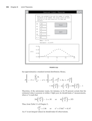
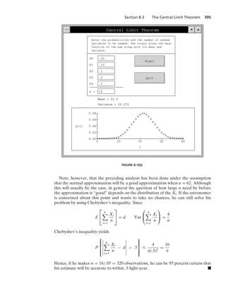
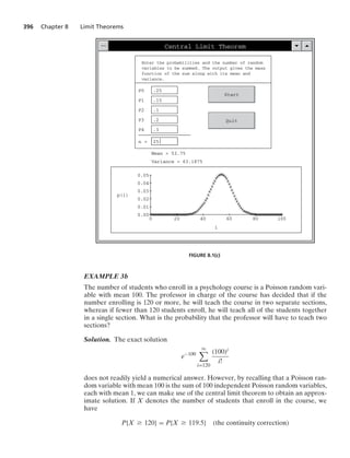
412. Section 8.3 The Central Limit Theorem 397
Central Limit Theorem
Enter the probabilities and the number of random
variables to be summed. The output gives the mass
function of the sum along with its mean and
variance.
P0 .25
P1 .15
P2 .1
P3 .2
P4 .3
n = 100
Start
Quit
Mean = 215.
Variance = 252.75
400
0
i
0.000
0.030
p(i)
300
200
100
0.025
0.020
0.015
0.010
0.005
FIGURE 8.1(d)
= P
0
X − 100
√
100
Ú
119.5 − 100
√
100
7
L 1 − (1.95)
L .0256
where we have used the fact that the variance of a Poisson random variable is equal
to its mean. .
EXAMPLE 3c
If 10 fair dice are rolled, find the approximate probability that the sum obtained is
between 30 and 40, inclusive.
Solution. Let Xi denote the value of the ith die, i = 1, 2, ... , 10. Since
E(Xi) =
7
2
, Var(Xi) = E[X2
i ] − (E[Xi])2
=
35
12
,

413. 398 Chapter 8 Limit Theorems
the central limit theorem yields
P{29.5 … X … 40.5} = P
⎧
⎪
⎪
⎪
⎨
⎪
⎪
⎪
⎩
29.5 − 35
@
350
12
…
X − 35
@
350
12
…
40.5 − 35
@
350
12
⎫
⎪
⎪
⎪
⎬
⎪
⎪
⎪
⎭
L 2 (1.0184) − 1
L .692 .
EXAMPLE 3d
Let Xi, i = 1, ... , 10, be independent random variables, each uniformly distributed
over (0, 1). Calculate an approximation to P
0
10
i=1
Xi 6
7
.
Solution. Since E[Xi] = 1
2 and Var(Xi) = 1
12 , we have, by the central limit theorem,
P
⎧
⎨
⎩
10
1
Xi 6
⎫
⎬
⎭
= P
⎧
⎪
⎪
⎪
⎪
⎪
⎪
⎨
⎪
⎪
⎪
⎪
⎪
⎪
⎩
10
1
Xi − 5
@
10(
1
12
)
6 − 5
@
10(
1
12
)
⎫
⎪
⎪
⎪
⎪
⎪
⎪
⎬
⎪
⎪
⎪
⎪
⎪
⎪
⎭
L 1 − (
√
1.2)
L .1367
Hence,
10
i=1
Xi will be greater than 6 only 14 percent of the time. .
EXAMPLE 3e
An instructor has 50 exams that will be graded in sequence. The times required to
grade the 50 exams are independent, with a common distribution that has mean
20 minutes and standard deviation 4 minutes. Approximate the probability that the
instructor will grade at least 25 of the exams in the first 450 minutes of work.
Solution. If we let Xi be the time that it takes to grade exam i, then
X =
25
i=1
Xi
is the time it takes to grade the first 25 exams. Because the instructor will grade at
least 25 exams in the first 450 minutes of work if the time it takes to grade the first 25
exams is less than or equal to 450, we see that the desired probability is P{X … 450}.
To approximate this probability, we use the central limit theorem. Now,
E[X] =
25
i=1
E[Xi] = 25(20) = 500
and
Var(X) =
25
i=1
Var(Xi) = 25(16) = 400

414. Section 8.3 The Central Limit Theorem 399
Consequently, with Z being a standard normal random variable, we have
P{X … 450} = P{
X − 500
√
400
…
450 − 500
√
400
}
L P{Z … −2.5}
= P{Z Ú 2.5}
= 1 − (2.5) = .006 .
Central limit theorems also exist when the Xi are independent, but not necessarily
identically distributed random variables. One version, by no means the most general,
is as follows.
Theorem 3.2 Central limit theorem for independent random variables
Let X1, X2, ... be a sequence of independent random variables having respective
means and variances μi = E[Xi], σ2
i = Var(Xi). If (a) the Xi are uniformly
bounded—that is, if for some M, P{|Xi| M}=1 for all i, and (b)
q
i=1
σ2
i =q—then
P
⎧
⎪
⎪
⎪
⎪
⎪
⎪
⎪
⎨
⎪
⎪
⎪
⎪
⎪
⎪
⎪
⎩
n
i=1
(Xi − μi)
A
B
B
C
n
i=1
σ2
i
… a
⎫
⎪
⎪
⎪
⎪
⎪
⎪
⎪
⎬
⎪
⎪
⎪
⎪
⎪
⎪
⎪
⎭
→ (a) as n → q
Historical Note
Pierre-Simon, Marquis de Laplace
The central limit theorem was originally stated and proven by the French math-
ematician Pierre-Simon, Marquis de Laplace, who came to the theorem from his
observations that errors of measurement (which can usually be regarded as being
the sum of a large number of tiny forces) tend to be normally distributed. Laplace,
who was also a famous astronomer (and indeed was called “the Newton of France”),
was one of the great early contributors to both probability and statistics. Laplace
was also a popularizer of the uses of probability in everyday life. He strongly believed
in its importance, as is indicated by the following quotations of his taken from his
published book Analytical Theory of Probability: “We see that the theory of proba-
bility is at bottom only common sense reduced to calculation; it makes us appreciate
with exactitude what reasonable minds feel by a sort of instinct, often without being
able to account for it.... It is remarkable that this science, which originated in the
consideration of games of chance, should become the most important object of
human knowledge.... The most important questions of life are, for the most part,
really only problems of probability.”
The application of the central limit theorem to show that measurement errors
are approximately normally distributed is regarded as an important contribution to
science. Indeed, in the 17th and 18th centuries the central limit theorem was often
called the law of frequency of errors. Listen to the words of Francis Galton (taken
from his book Natural Inheritance, published in 1889): “I know of scarcely anything
so apt to impress the imagination as the wonderful form of cosmic order expressed
by the ‘Law of Frequency of Error.’ The Law would have been personified by the
Greeks and deified, if they had known of it. It reigns with serenity and in complete
self-effacement amidst the wildest confusion. The huger the mob and the greater the
apparent anarchy, the more perfect is its sway. It is the supreme law of unreason.”

415. 400 Chapter 8 Limit Theorems
8.4 THE STRONG LAW OF LARGE NUMBERS
The strong law of large numbers is probably the best-known result in probability the-
ory. It states that the average of a sequence of independent random variables having
a common distribution will, with probability 1, converge to the mean of that distribu-
tion.
Theorem 4.1 The strong law of large numbers
Let X1, X2, ... be a sequence of independent and identically distributed random vari-
ables, each having a finite mean μ = E[Xi]. Then, with probability 1,
X1 + X2 + · · · + Xn
n
→μ as n → q†
As an application of the strong law of large numbers, suppose that a sequence of
independent trials of some experiment is performed. Let E be a fixed event of the
experiment, and denote by P(E) the probability that E occurs on any particular trial.
Letting
Xi =
%
1 if E occurs on the ith trial
0 if E does not occur on the ith trial
we have, by the strong law of large numbers, that with probability 1,
X1 + · · · + Xn
n
→ E[X] = P(E) (4.1)
Since X1 + · · · + Xn represents the number of times that the event E occurs in the
first n trials, we may interpret Equation (4.1) as stating that, with probability 1, the
limiting proportion of time that the event E occurs is just P(E).
Although the theorem can be proven without this assumption, our proof of the
strong law of large numbers will assume that the random variables Xi have a finite
fourth moment. That is, we will suppose that E[X4
i ] = K q.
Proof of the Strong Law of Large Numbers: To begin, assume that μ, the mean of
the Xi, is equal to 0. Let Sn =
n
i=1
Xi and consider
E[S4
n] = E[(X1 + · · · + Xn)(X1 + · · · + Xn)
* (X1 + · · · + Xn)(X1 + · · · + Xn)]
Expanding the right side of the preceding equation results in terms of the form
X4
i , X3
i Xj, X2
i X2
j , X2
i XjXk, and XiXjXkXl
where i, j, k, and l are all different. Because all the Xi have mean 0, it follows by
independence that
E[X3
i Xj] = E[X3
i ]E[Xj] = 0
E[X2
i XjXk] = E[X2
i ]E[Xj]E[Xk] = 0
E[XiXjXkXl] = 0
†That is, the strong law of large numbers states that
P{ lim
n→q
(X1 + · · · + Xn)/n = μ} = 1

416. Section 8.4 The Strong Law of Large Numbers 401
Now, for a given pair i and j, there will be
4
2
= 6 terms in the expansion that will
equal X2
i X2
j . Hence, upon expanding the preceding product and taking expectations
term by term, it follows that
E[S4
n] = nE[X4
i ] + 6
n
2
E[X2
i X2
j ]
= nK + 3n(n − 1)E[X2
i ]E[X2
j ]
where we have once again made use of the independence assumption. Now, since
0 … Var(X2
i ) = E[X4
i ] − (E[X2
i ])2
we have
(E[X2
i ])2
… E[X4
i ] = K
Therefore, from the preceding, we obtain
E[S4
n] … nK + 3n(n − 1)K
which implies that
E
S4
n
n4
…
K
n3
+
3K
n2
Therefore,
E
⎡
⎣
q
n=1
S4
n
n4
⎤
⎦ =
q
n=1
E
S4
n
n4
q
But the preceding implies that, with probability 1,
q
n=1
S4
n/n4 q. (For if there is a
positive probability that the sum is infinite, then its expected value is infinite.) But the
convergence of a series implies that its nth term goes to 0; so we can conclude that,
with probability 1,
lim
n→q
S4
n
n4
= 0
But if S4
n/n4 = (Sn/n)4 goes to 0, then so must Sn/n; hence, we have proven that, with
probability 1,
Sn
n
→ 0 as n → q
When μ, the mean of the Xi, is not equal to 0, we can apply the preceding argument
to the random variables Xi − μ to obtain that with probability 1,
lim
n→q
n
i=1
(Xi − μ)
n
= 0
or, equivalently,
lim
n→q
n
i=1
Xi
n
= μ
which proves the result.

417. 402 Chapter 8 Limit Theorems
The strong law is illustrated by two modules on the text website that consider inde-
pendent and identically distributed random variables which take on one of the values
0, 1, 2, 3, and 4. The modules simulate the values of n such random variables; the
proportions of time that each outcome occurs, as well as the resulting sample mean
n
i=1
Xi/n, are then indicated and plotted. When using these modules, which differ only
in the type of graph presented, one enters the probabilities and the desired value of n.
Figure 8.2 gives the results of a simulation using a specified probability mass function
and (a) n = 100, (b) n = 1000, and (c) n = 10,000.
Many students are initially confused about the difference between the weak and
the strong laws of large numbers. The weak law of large numbers states that, for any
specified large value n∗, (X1 + · · · + Xn∗ )/n∗ is likely to be near μ. However, it does
not say that (X1 + · · · + Xn)/n is bound to stay near μ for all values of n larger than
n∗. Thus, it leaves open the possibility that large values of |(X1 + · · · + Xn)/n − μ|
can occur infinitely often (though at infrequent intervals). The strong law shows that
this cannot occur. In particular, it implies that, with probability 1, for any positive
value ε, 6
6
6
6
6
6
n
1
Xi
n
− μ
6
6
6
6
6
6
will be greater than ε only a finite number of times.
Strong Law Of Large Numbers
Enter the probabilities and the number of trials
to be simulated. The output gives the total number
of times each outcome occurs, and the average
of all outcomes.
P0 .1
P1 .2
P2 .3
P3 .35
P4 .05
n = 100
Start
Quit
Theoretical Mean = 2.05
Sample Mean = 1.89
0
15
1
20
2
30
3
31
4
4
FIGURE 8.2(a)

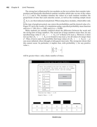
418. Section 8.5 Other Inequalities 403
Strong Law Of Large Numbers
Enter the probabilities and the number of trials
to be simulated. The output gives the total number
of times each outcome occurs, and the average
of all outcomes.
P0 .1
P1 .2
P2 .3
P3 .35
P4 .05
n = 1000
Start
Quit
Theoretical Mean = 2.05
Sample Mean = 2.078
0
106
1
189
2
285
3
361
4
59
FIGURE 8.2(b)
The strong law of large numbers was originally proven, in the special case of
Bernoulli random variables, by the French mathematician Borel. The general form of
the strong law presented in Theorem 4.1 was proven by the Russian mathematician
A. N. Kolmogorov.
8.5 OTHER INEQUALITIES
We are sometimes confronted with situations in which we are interested in obtaining
an upper bound for a probability of the form P{X − μ Ú a}, where a is some positive
value and when only the mean μ = E[X] and variance σ2 = Var(X) of the distribu-
tion of X are known. Of course, since X − μ Ú a 0 implies that |X − μ| Ú a, it
follows from Chebyshev’s inequality that
P{X − μ Ú a} … P{|X − μ| Ú a} …
σ2
a2
when a 0
However, as the following proposition shows, it turns out that we can do better.
Proposition 5.1. One-sided Chebyshev inequality
If X is a random variable with mean 0 and finite variance σ2, then, for any a 0,
P{X Ú a} …
σ2
σ2 + a2

419. 404 Chapter 8 Limit Theorems
Strong Law Of Large Numbers
Enter the probabilities and the number of trials
to be simulated. The output gives the total number
of times each outcome occurs, and the average
of all outcomes.
P0 .1
P1 .2
P2 .3
P3 .35
P4 .05
n = 10000
Start
Quit
Theoretical Mean = 2.05
Sample Mean = 2.0416
0
1041
1
2027
2
2917
3
3505
4
510
FIGURE 8.2(c)
Proof. Let b 0 and note that
X Ú a is equivalent to X + b Ú a + b
Hence,
P{X Ú a} = P{X + b Ú a + b}
… P{(X + b)2
Ú (a + b)2
}
where the inequality is obtained by noting that since a + b 0, X + b Ú a + b
implies that (X + b)2 Ú (a + b)2. Upon applying Markov’s inequality, the
preceding yields that
P{X Ú a} …
E[(X + b)2]
(a + b)2
=
σ2 + b2
(a + b)2
Letting b = σ2/a [which is easily seen to be the value of b that minimizes
(σ2 + b2)/(a + b)2] gives the desired result.

420. Section 8.5 Other Inequalities 405
EXAMPLE 5a
If the number of items produced in a factory during a week is a random variable with
mean 100 and variance 400, compute an upper bound on the probability that this
week’s production will be at least 120.
Solution. It follows from the one-sided Chebyshev inequality that
P{X Ú 120} = P{X − 100 Ú 20} …
400
400 + (20)2
=
1
2
Hence, the probability that this week’s production will be 120 or more is at most 1
2 .
If we attempted to obtain a bound by applying Markov’s inequality, then we would
have obtained
P{X Ú 120} …
E(X)
120
=
5
6
which is a far weaker bound than the preceding one. .
Suppose now that X has mean μ and variance σ2. Since both X − μ and μ − X
have mean 0 and variance σ2, it follows from the one-sided Chebyshev inequality
that, for a 0,
P{X − μ Ú a} …
σ2
σ2 + a2
and
P{μ − X Ú a} …
σ2
σ2 + a2
Thus, we have the following corollary.
Corollary 5.1. If E[X] = μ and Var(X) = σ2, then, for a 0,
P{X Ú μ + a} …
σ2
σ2 + a2
P{X … μ − a} …
σ2
σ2 + a2
EXAMPLE 5b
A set of 200 people consisting of 100 men and 100 women is randomly divided into
100 pairs of 2 each. Give an upper bound to the probability that at most 30 of these
pairs will consist of a man and a woman.
Solution. Number the men arbitrarily from 1 to 100, and for i = 1, 2, ... 100, let
Xi =
%
1 if man i is paired with a woman
0 otherwise
Then X, the number of man–woman pairs, can be expressed as
X =
100
i=1
Xi

421. 406 Chapter 8 Limit Theorems
Because man i is equally likely to be paired with any of the other 199 people, of which
100 are women, we have
E[Xi] = P{Xi = 1} =
100
199
Similarly, for i Z j,
E[XiXj] = P{Xi = 1, Xj = 1}
= P{Xi = 1}P{Xj = 1|Xi = 1} =
100
199
99
197
where P{Xj = 1|Xi = 1} = 99/197, since, given that man i is paired with a woman,
man j is equally likely to be paired with any of the remaining 197 people, of which 99
are women. Hence, we obtain
E[X] =
100
i=1
E[Xi]
= (100)
100
199
L 50.25
Var(X) =
100
i=1
Var(Xi) + 2
ij
Cov(Xi, Xj)
= 100
100
199
99
199
+ 2
100
2
100
199
99
197
−
100
199
2
L 25.126
The Chebyshev inequality then yields
P{X … 30} … P{|X − 50.25| Ú 20.25} …
25.126
(20.25)2
L .061
Thus, there are fewer than 6 chances in a hundred that fewer than 30 men will be
paired with women. However, we can improve on this bound by using the one-sided
Chebyshev inequality, which yields
P{X … 30} = P{X … 50.25 − 20.25}
…
25.126
25.126 + (20.25)2
L .058 .
When the moment generating function of the random variable X is known, we can
obtain even more effective bounds on P{X Ú a}. Let
M(t) = E[etX
]
be the moment generating function of the random variable X. Then, for t 0,
P{X Ú a} = P{etX
Ú eta
}
… E[etX
]e−ta
by Markov’s inequality

422. Section 8.5 Other Inequalities 407
Similarly, for t 0,
P{X … a} = P{etX
Ú eta
}
… E[etX
]e−ta
Thus, we have the following inequalities, known as Chernoff bounds.
Proposition 5.2. Chernoff bounds
P{X Ú a} … e−ta
M(t) for all t 0
P{X … a} … e−ta
M(t) for all t 0
Since the Chernoff bounds hold for all t in either the positive or negative quadrant,
we obtain the best bound on P{X Ú a} by using the t that minimizes e−taM(t).
EXAMPLE 5c Chernoff bounds for the standard normal random variable
If Z is a standard normal random variable, then its moment generating function is
M(t) = et2/2, so the Chernoff bound on P{Z Ú a} is given by
P{Z Ú a} … e−ta
et2/2
for all t 0
Now the value of t, t 0, that minimizes et2/2−ta is the value that minimizes t2/2 − ta,
which is t = a. Thus, for a 0, we have
P{Z Ú a} … e−a2/2
Similarly, we can show that, for a 0,
P{Z … a} … e−a2/2
.
EXAMPLE 5d Chernoff bounds for the Poisson random variable
If X is a Poisson random variable with parameter λ, then its moment generating func-
tion is M(t) = eλ(et−1). Hence, the Chernoff bound on P{X Ú i} is
P{X Ú i} … eλ(et−1)
e−it
t 0
Minimizing the right side of the preceding inequality is equivalent to minimizing
λ(et − 1) − it, and calculus shows that the minimal value occurs when et = i/λ. Pro-
vided that i/λ 1, this minimizing value of t will be positive. Therefore, assuming
that i λ and letting et = i/λ in the Chernoff bound yields
P{X Ú i} … eλ(i/λ−1)
λ
i
i
or, equivalently,
P{X Ú i} …
e−λ(eλ)i
ii
.
EXAMPLE 5e
Consider a gambler who is equally likely to either win or lose 1 unit on every play,
independently of his past results. That is, if Xi is the gambler’s winnings on the ith
play, then the Xi are independent and

423. 408 Chapter 8 Limit Theorems
P{Xi = 1} = P{Xi = −1} =
1
2
Let Sn =
n
i=1
Xi denote the gambler’s winnings after n plays. We will use the Chernoff
bound on P{Sn Ú a}. To start, note that the moment generating function of Xi is
E[etX
] =
et + e−t
2
Now, using the McLaurin expansions of et and e−t, we see that
et
+ e−t
= 1 + t +
t2
2!
+
t3
3!
+ · · · +
1 − t +
t2
2!
−
t3
3!
+ · · ·
= 2
0
1 +
t2
2!
+
t4
4!
+ · · ·
7
= 2
q
n=0
t2n
(2n)!
… 2
q
n=0
(t2/2)n
n!
since (2n)! Ú n!2n
= 2et2/2
Therefore,
E[etX
] Ú et2/2
Since the moment generating function of the sum of independent random variables
is the product of their moment generating functions, we have
E[etSn ] = (E[etX
])n
… ent2/2
Using the preceding result along with the Chernoff bound gives
P{Sn Ú a} … e−ta
ent2/2
t 0
The value of t that minimizes the right side of the preceding is the value that min-
imizes nt2/2 − ta, and this value is t = a/n. Supposing that a 0 (so that the
minimizing t is positive) and letting t = a/n in the preceding inequality yields
P{Sn Ú a} … e−a2/2n
a 0
This latter inequality yields, for example,
P{S10 Ú 6} … e−36/20
L .1653

424. Section 8.5 Other Inequalities 409
whereas the exact probability is
P{S10 Ú 6} = P{gambler wins at least 8 of the first 10 games}
=
10
8
+
10
9
+
10
10
210
=
56
1024
L .0547 .
The next inequality is one having to do with expectations rather than probabilities.
Before stating it, we need the following definition.
Definition
A twice-differentiable real-valued function f(x) is said to be convex if f(x) Ú 0 for
all x; similarly, it is said to be concave if f(x) … 0.
Some examples of convex functions are f(x) = x2, f(x) = eax, and f(x) = −x1/n for
x Ú 0. If f(x) is convex, then g(x) = −f(x) is concave, and vice versa.
Proposition 5.3. Jensen’s inequality
If f(x) is a convex function, then
E[ f(X)] Ú f(E[X])
provided that the expectations exist and are finite.
Proof. Expanding f(x) in a Taylor’s series expansion about μ = E[X] yields
f(x) = f(μ) + f
(μ)(x − μ) +
f(ξ)(x − μ)2
2
where ξ is some value between x and μ. Since f(ξ) Ú 0, we obtain
f(x) Ú f(μ) + f
(μ)(x − μ)
Hence,
f(X) Ú f(μ) + f
(μ)(X − μ)
Taking expectations yields
E[ f(X)] Ú f(μ) + f
(μ)E[X − μ] = f(μ)
and the inequality is established.
EXAMPLE 5f
An investor is faced with the following choices: Either she can invest all of her money
in a risky proposition that would lead to a random return X that has mean m, or
she can put the money into a risk-free venture that will lead to a return of m with
probability 1. Suppose that her decision will be made on the basis of maximizing the
expected value of u(R), where R is her return and u is her utility function. By Jensen’s
inequality, it follows that if u is a concave function, then E[u(X)] … u(m), so the risk-
free alternative is preferable, whereas if u is convex, then E[u(X)] Ú u(m), so the
risky investment alternative would be preferred. .

425. 410 Chapter 8 Limit Theorems
8.6 BOUNDING THE ERROR PROBABILITY WHEN APPROXIMATING A SUM OF INDEPENDENT
BERNOULLI RANDOM VARIABLES BY A POISSON RANDOM VARIABLE
In this section, we establish bounds on how closely a sum of independent Bernoulli
random variables is approximated by a Poisson random variable with the same mean.
Suppose that we want to approximate the sum of independent Bernoulli random
variables with respective means p1, p2, ... , pn. Starting with a sequence Y1, ... , Yn
of independent Poisson random variables, with Yi having mean pi, we will construct
a sequence of independent Bernoulli random variables X1, ... , Xn with parameters
p1, ... , pn such that
P{Xi Z Yi} … p2
i for each i
Letting X =
n
i=1
Xi and Y =
n
i=1
Yi, we will use the preceding inequality to con-
clude that
P{X Z Y} …
n
i=1
p2
i
Finally, we will show that the preceding inequality implies that, for any set of real
numbers A,
|P{X ∈ A} − P{Y ∈ A}| …
n
i=1
p2
i
Since X is the sum of independent Bernoulli random variables and Y is a Poisson
random variable, the latter inequality will yield the desired bound.
To show how the task is accomplished, let Yi, i = 1, ... , n be independent Pois-
son random variables with respective means pi. Now let U1, ... , Un be independent
random variables that are also independent of the Yi’s and which are such that
Ui =
%
0 with probability (1 − pi)epi
1 with probability 1 − (1 − pi)epi
This definition implicitly makes use of the inequality
e−p
Ú 1 − p
in assuming that (1 − pi)epi … 1.
Next, define the random variables Xi, i = 1, ... , n, by
Xi =
%
0 if Yi = Ui = 0
1 otherwise
Note that
P{Xi = 0} = P{Yi = 0}P{Ui = 0} = e−pi (1 − pi)epi = 1 − pi
P{Xi = 1} = 1 − P{Xi = 0} = pi

426. Section 8.6 Bounding the Error Probability 411
Now, if Xi is equal to 0, then so must Yi equal 0 (by the definition of Xi). Therefore,
P{Xi Z Yi} = P{Xi = 1, Yi Z 1}
= P{Yi = 0, Xi = 1} + P{Yi 1}
= P{Yi = 0, Ui = 1} + P{Yi 1}
= e−pi [1 − (1 − pi)epi ] + 1 − e−pi − pie−pi
= pi − pie−pi
… p2
i (since 1 − e−p
… p)
Now let X =
n
i=1
Xi and Y =
n
i=1
Yi, and note that X is the sum of independent
Bernoulli random variables and Y is Poisson with the expected value E[Y] = E[X] =
n
i=1
pi. Note also that the inequality X Z Y implies that Xi Z Yi for some i, so
P{X Z Y} … P{Xi Z Yi for some i}
…
n
i=1
P{Xi Z Yi} (Boole’s inequality)
…
n
i=1
p2
i
For any event B, let IB, the indicator variable for the event B, be defined by
IB =
%
1 if B occurs
0 otherwise
Note that, for any set of real numbers A,
I{X∈A} − I{Y∈A} … I{XZY}
The preceding inequality follows from the fact that, since an indicator variable is
either 0 or 1, the left-hand side equals 1 only when I{X∈A} = 1 and I{Y∈A} = 0. But
this would imply that X ∈ A and Y ∈ A, which means that X Z Y, so the right side
would also equal 1. Upon taking expectations of the preceding inequality, we obtain
P{X ∈ A} − P{Y ∈ A} … P{X Z Y}
By reversing X and Y, we obtain, in the same manner,
P{Y ∈ A} − P{X ∈ A} … P{X Z Y}
Thus, we can conclude that
|P{X ∈ A} − P{Y ∈ A}| … P{X Z Y}
Therefore, we have proven that with λ =
n
i=1
pi,
6
6
6
6
6
6
6
P
⎧
⎨
⎩
n
i=1
Xi ∈ A
⎫
⎬
⎭
−
i∈A
e−λλi
i!
6
6
6
6
6
6
6
…
n
i=1
p2
i

427. 412 Chapter 8 Limit Theorems
Remark. When all the pi are equal to p, X is a binomial random variable. Hence,
the preceding inequality shows that, for any set of nonnegative integers A,
6
6
6
6
6
6
i∈A
n
i
pi
(1 − p)n−i
−
i∈A
e−np(np)i
i!
6
6
6
6
6
6
… np2
.
SUMMARY
Two useful probability bounds are provided by the Markov and Chebyshev inequali-
ties. The Markov inequality is concerned with nonnegative random variables and says
that, for X of that type,
P{X Ú a} …
E[X]
a
for every positive value a. The Chebyshev inequality, which is a simple consequence
of the Markov inequality, states that if X has mean μ and variance σ2, then, for every
positive k,
P{|X − μ| Ú kσ} …
1
k2
The two most important theoretical results in probability are the central limit theorem
and the strong law of large numbers. Both are concerned with a sequence of indepen-
dent and identically distributed random variables. The central limit theorem says that
if the random variables have a finite mean μ and a finite variance σ2, then the distri-
bution of the sum of the first n of them is, for large n, approximately that of a normal
random variable with mean nμ and variance nσ2. That is, if Xi, i Ú 1, is the sequence,
then the central limit theorem states that, for every real number a,
lim
n→q
P
0
X1 + · · · + Xn − nμ
σ
√
n
… a
7
=
1
√
2π
* a
−q
e−x2/2
dx
The strong law of large numbers requires only that the random variables in the sequence
have a finite mean μ. It states that, with probability 1, the average of the first n of them
will converge to μ as n goes to infinity. This implies that if A is any specified event
of an experiment for which independent replications are performed, then the limit-
ing proportion of experiments whose outcomes are in A will, with probability 1, equal
P(A). Therefore, if we accept the interpretation that “with probability 1” means “with
certainty,” we obtain the theoretical justification for the long-run relative frequency
interpretation of probabilities.
PROBLEMS
8.1. Suppose that X is a random variable with mean
and variance both equal to 20. What can be said
about P{0 X 40}?
8.2. From past experience, a professor knows that the
test score of a student taking her final examination
is a random variable with mean 75.
(a) Give an upper bound for the probability that
a student’s test score will exceed 85. Sup-
pose, in addition, that the professor knows
that the variance of a student’s test score is
equal to 25.
(b) What can be said about the probability that a
student will score between 65 and 85?
(c) How many students would have to take the
examination to ensure, with probability at
least .9, that the class average would be
within 5 of 75? Do not use the central limit
theorem.

428. Problems 413
8.3. Use the central limit theorem to solve part (c) of
Problem 2.
8.4. Let X1, ... , X20 be independent Poisson random
variables with mean 1.
(a) Use the Markov inequality to obtain a
bound on
P
⎧
⎨
⎩
20
1
Xi 15
⎫
⎬
⎭
(b) Use the central limit theorem to approximate
P
⎧
⎨
⎩
20
1
Xi 15
⎫
⎬
⎭
.
8.5. Fifty numbers are rounded off to the nearest inte-
ger and then summed. If the individual round-
off errors are uniformly distributed over (−.5, .5),
approximate the probability that the resultant sum
differs from the exact sum by more than 3.
8.6. A die is continually rolled until the total sum of
all rolls exceeds 300. Approximate the probability
that at least 80 rolls are necessary.
8.7. A person has 100 light bulbs whose lifetimes are
independent exponentials with mean 5 hours. If
the bulbs are used one at a time, with a failed bulb
being replaced immediately by a new one, approx-
imate the probability that there is still a working
bulb after 525 hours.
8.8. In Problem 7, suppose that it takes a random time,
uniformly distributed over (0, .5), to replace a
failed bulb. Approximate the probability that all
bulbs have failed by time 550.
8.9. If X is a gamma random variable with parameters
(n, 1), approximately how large need n be so that
P
06
6
6
6
X
n
− 1
6
6
6
6 .01
7
.01?
8.10. Civil engineers believe that W, the amount of
weight (in units of 1000 pounds) that a certain span
of a bridge can withstand without structural dam-
age resulting, is normally distributed with mean
400 and standard deviation 40. Suppose that the
weight (again, in units of 1000 pounds) of a car
is a random variable with mean 3 and standard
deviation .3. Approximately how many cars would
have to be on the bridge span for the probability
of structural damage to exceed .1?
8.11. Many people believe that the daily change of price
of a company’s stock on the stock market is a ran-
dom variable with mean 0 and variance σ2. That
is, if Yn represents the price of the stock on the nth
day, then
Yn = Yn−1 + Xn n Ú 1
where X1, X2, ... are independent and identically
distributed random variables with mean 0 and
variance σ2. Suppose that the stock’s price today
is 100. If σ2 = 1, what can you say about the prob-
ability that the stock’s price will exceed 105 after
10 days?
8.12. We have 100 components that we will put in use in
a sequential fashion. That is, component 1 is ini-
tially put in use, and upon failure, it is replaced
by component 2, which is itself replaced upon fail-
ure by component 3, and so on. If the lifetime
of component i is exponentially distributed with
mean 10 + i/10, i = 1, ... , 100, estimate the prob-
ability that the total life of all components will
exceed 1200. Now repeat when the life distribu-
tion of component i is uniformly distributed over
(0, 20 + i/5), i = 1, ... , 100.
8.13. Student scores on exams given by a certain instruc-
tor have mean 74 and standard deviation 14. This
instructor is about to give two exams, one to a class
of size 25 and the other to a class of size 64.
(a) Approximate the probability that the average
test score in the class of size 25 exceeds 80.
(b) Repeat part (a) for the class of size 64.
(c) Approximate the probability that the average
test score in the larger class exceeds that of
the other class by over 2.2 points.
(d) Approximate the probability that the average
test score in the smaller class exceeds that of
the other class by over 2.2 points.
8.14. A certain component is critical to the operation of
an electrical system and must be replaced immedi-
ately upon failure. If the mean lifetime of this type
of component is 100 hours and its standard devi-
ation is 30 hours, how many of these components
must be in stock so that the probability that the
system is in continual operation for the next 2000
hours is at least .95?
8.15. An insurance company has 10,000 automobile pol-
icyholders. The expected yearly claim per policy-
holder is $240, with a standard deviation of $800.
Approximate the probability that the total yearly
claim exceeds $2.7 million.
8.16. A.J. has 20 jobs that she must do in sequence, with
the times required to do each of these jobs being
independent random variables with mean 50 min-
utes and standard deviation 10 minutes. M.J. has
20 jobs that he must do in sequence, with the times
required to do each of these jobs being indepen-
dent random variables with mean 52 minutes and
standard deviation 15 minutes.
(a) Find the probability that A.J. finishes in less
than 900 minutes.
(b) Find the probability that M.J. finishes in less
than 900 minutes.
(c) Find the probability that A.J. finishes
before M.J.

429. 414 Chapter 8 Limit Theorems
8.17. Redo Example 5b under the assumption that the
number of man–woman pairs is (approximately)
normally distributed. Does this seem like a reason-
able supposition?
8.18. Repeat part (a) of Problem 2 when it is known that
the variance of a student’s test score is equal to 25.
8.19. A lake contains 4 distinct types of fish. Suppose
that each fish caught is equally likely to be any
one of these types. Let Y denote the number of
fish that need be caught to obtain at least one of
each type.
(a) Give an interval (a, b) such that P{a … Y … b}
Ú .90.
(b) Using the one-sided Chebyshev inequality,
how many fish need we plan on catching so as
to be at least 90 percent certain of obtaining
at least one of each type.
8.20. If X is a nonnegative random variable with mean
25, what can be said about
(a) E[X3]?
(b) E[
√
X]?
(c) E[log X]?
(d) E[e−X]?
8.21. Let X be a nonnegative random variable.
Prove that
E[X] … (E[X2
])1/2
… (E[X3
])1/3
… · · ·
8.22. Would the results of Example 5f change if the
investor were allowed to divide her money and
invest the fraction α, 0 α 1, in the risky propo-
sition and invest the remainder in the risk-free
venture? Her return for such a split investment
would be R = αX + (1 − α)m.
8.23. Let X be a Poisson random variable with mean 20.
(a) Use the Markov inequality to obtain an upper
bound on
p = P{X Ú 26}
(b) Use the one-sided Chebyshev inequality to
obtain an upper bound on p.
(c) Use the Chernoff bound to obtain an upper
bound on p.
(d) Approximate p by making use of the central
limit theorem.
(e) Determine p by running an appropriate pro-
gram.
THEORETICAL EXERCISES
8.1. If X has variance σ2, then σ, the positive square
root of the variance, is called the standard devia-
tion. If X has mean μ and standard deviation σ,
show that
P{|X − μ| Ú kσ} …
1
k2
8.2. If X has mean μ and standard deviation σ, the
ratio r K |μ|/σ is called the measurement signal-
to-noise ratio of X. The idea is that X can be
expressed as X = μ + (X − μ), with μ represent-
ing the signal and X − μ the noise. If we define
|(X − μ)/μ| K D as the relative deviation of X
from its signal (or mean) μ, show that, for α 0,
P{D … α} Ú 1 −
1
r2α2
8.3. Compute the measurement signal-to-noise ratio—
that is, |μ|/σ, where μ = E[X] and σ2 = Var(X)—
of the following random variables:
(a) Poisson with mean λ;
(b) binomial with parameters n and p;
(c) geometric with mean 1/p;
(d) uniform over (a, b);
(e) exponential with mean 1/λ;
(f) normal with parameters μ, σ2.
8.4. Let Zn, n Ú 1, be a sequence of random variables
and c a constant such that, for each ε 0, P{|Zn −
c| ε} → 0 as n → q. Show that, for any bounded
continuous function g,
E[g(Zn)] → g(c) as n→q
8.5. Let f(x) be a continuous function defined for 0 …
x … 1. Consider the functions
Bn(x) =
n
k=0
f
k
n
n
k
xk
(1 − x)n−k
(called Bernstein polynomials) and prove that
lim
n→q
Bn(x) = f(x)
Hint: Let X1, X2, ... be independent Bernoulli
random variables with mean x. Show that
Bn(x) = E
f
X1 + · · · + Xn
n
and then use Theoretical Exercise 4.
Since it can be shown that the convergence of
Bn(x) to f(x) is uniform in x, the preceding rea-
soning provides a probabilistic proof of the famous
Weierstrass theorem of analysis, which states that

430. Self-Test Problems and Exercises 415
any continuous function on a closed interval can be
approximated arbitrarily closely by a polynomial.
8.6. (a) Let X be a discrete random variable whose
possible values are 1, 2, ... . If P{X = k} is
nonincreasing in k = 1, 2, ... , prove that
P{X = k} … 2
E[X]
k2
(b) Let X be a nonnegative continuous random
variable having a nonincreasing density func-
tion. Show that
f(x) …
2E[X]
x2
for all x 0
8.7. Suppose that a fair die is rolled 100 times. Let Xi
be the value obtained on the ith roll. Compute an
approximation for
P
⎧
⎨
⎩
100
1
Xi … a100
⎫
⎬
⎭
1 a 6
8.8. Explain why a gamma random variable with
parameters (t, λ) has an approximately normal dis-
tribution when t is large.
8.9. Suppose a fair coin is tossed 1000 times. If the first
100 tosses all result in heads, what proportion of
heads would you expect on the final 900 tosses?
Comment on the statement “The strong law of
large numbers swamps, but does not compensate.”
8.10. If X is a Poisson random variable with mean λ,
show that for i λ,
P{X … i} …
e−λ(eλ)i
ii
8.11. Let X be a binomial random variable with param-
eters n and p. Show that, for i np,
(a) minimum
t0
e−tiE[etX] occurs when t is such that
et = iq
(n−i)p , where q = 1 − p.
(b) P{X Ú i} … nn
ii(n−i)n−i pi(1 − p)n−i.
8.12. The Chernoff bound on a standard normal random
variable Z gives P{Z a} … e−a2/2, a 0. Show,
by considering the density of Z, that the right side
of the inequality can be reduced by the factor 2.
That is, show that
P{Z a} …
1
2
e−a2/2
a 0
8.13. Show that if E[X] 0 and θ Z 0 is such that
E[eθX] = 1, then θ 0.
SELF-TEST PROBLEMS AND EXERCISES
8.1. The number of automobiles sold weekly at a cer-
tain dealership is a random variable with expected
value 16. Give an upper bound to the probabil-
ity that
(a) next week’s sales exceed 18;
(b) next week’s sales exceed 25.
8.2. Suppose in Problem 1 that the variance of the
number of automobiles sold weekly is 9.
(a) Give a lower bound to the probability that
next week’s sales are between 10 and 22,
inclusively.
(b) Give an upper bound to the probability that
next week’s sales exceed 18.
8.3. If
E[X] = 75 E[Y] = 75 Var(X) = 10
Var(Y) = 12 Cov(X, Y) = −3
give an upper bound to
(a) P{|X − Y| 15};
(b) P{X Y + 15};
(c) P{Y X + 15}.
8.4. Suppose that the number of units produced daily
at factory A is a random variable with mean 20 and
standard deviation 3 and the number produced
at factory B is a random variable with mean
18 and standard deviation 6. Assuming indepen-
dence, derive an upper bound for the probability
that more units are produced today at factory B
than at factory A.
8.5. The amount of time that a certain type of compo-
nent functions before failing is a random variable
with probability density function
f(x) = 2x 0 x 1
Once the component fails, it is immediately
replaced by another one of the same type. If we
let Xi denote the lifetime of the ith component to
be put in use, then Sn =
n
i=1
Xi represents the time
of the nth failure. The long-term rate at which fail-
ures occur, call it r, is defined by
r = lim
n→q
n
Sn
Assuming that the random variables Xi, i Ú 1, are
independent, determine r.
8.6. In Self-Test Problem 5, how many compo-
nents would one need to have on hand to be

431. 416 Chapter 8 Limit Theorems
approximately 90 percent certain that the stock
will last at least 35 days?
8.7. The servicing of a machine requires two separate
steps, with the time needed for the first step being
an exponential random variable with mean .2 hour
and the time for the second step being an inde-
pendent exponential random variable with mean
.3 hour. If a repair person has 20 machines to ser-
vice, approximate the probability that all the work
can be completed in 8 hours.
8.8. On each bet, a gambler loses 1 with probability .7,
loses 2 with probability .2, or wins 10 with prob-
ability .1. Approximate the probability that the
gambler will be losing after his first 100 bets.
8.9. Determine t so that the probability that the repair
person in Self-Test Problem 7 finishes the 20 jobs
within time t is approximately equal to .95.
8.10. A tobacco company claims that the amount of
nicotine in one of its cigarettes is a random
variable with mean 2.2 mg and standard devia-
tion .3 mg. However, the average nicotine con-
tent of 100 randomly chosen cigarettes was 3.1
mg. Approximate the probability that the average
would have been as high as or higher than 3.1 if the
company’s claims were true.
8.11. Each of the batteries in a collection of 40 batter-
ies is equally likely to be either a type A or a type
B battery. Type A batteries last for an amount of
time that has mean 50 and standard deviation 15;
type B batteries last for an amount of time that has
mean 30 and standard deviation 6.
(a) Approximate the probability that the total life
of all 40 batteries exceeds 1700.
(b) Suppose it is known that 20 of the batteries
are type A and 20 are type B. Now approx-
imate the probability that the total life of all
40 batteries exceeds 1700.
8.12. A clinic is equally likely to have 2, 3, or 4 doctors
volunteer for service on a given day. No matter
how may volunteer doctors there are on a given
day, the numbers of patients seen by these doctors
are independent Poisson random variables with
mean 30. Let X denote the number of patients
seen in the clinic on a given day.
(a) Find E[X].
(b) Find Var(X).
(c) Use a table of the standard normal probability
distribution to approximate P{X 65}.
8.13. The strong law of large numbers states that, with
probability 1, the successive arithmetic averages
of a sequence of independent and identically dis-
tributed random variables converge to their com-
mon mean μ. What do the successive geometric
averages converge to? That is, what is
lim
n→q
(
n
i=1
Xi)1/n

432. C H A P T E R 9
Additional Topics in Probability
9.1 THE POISSON PROCESS
9.2 MARKOV CHAINS
9.3 SURPRISE, UNCERTAINTY, AND ENTROPY
9.4 CODING THEORY AND ENTROPY
9.1 THE POISSON PROCESS
Before we define a Poisson process, let us recall that a function f is said to be o(h) if
lim
h→0
f(h)
h
= 0.
That is, f is o(h) if, for small values of h, f(h) is small even in relation to h. Sup-
pose now that “events” are occurring at random points at time, and let N(t) denote
the number of events that occur in the time interval [0, t]. The collection of random
variables {N(t), t Ú 0} is said to be a Poisson process having rate λ, λ 0, if
(i) N(0) = 0.
(ii) The numbers of events that occur in disjoint time intervals are independent.
(iii) The distribution of the number of events that occur in a given interval depends
only on the length of that interval and not on its location.
(iv) P{N(h) = 1} = λh + o(h).
(v) P{N(h) Ú 2} = o(h).
Thus, condition (i) states that the process begins at time 0. Condition (ii), the inde-
pendent increment assumption, states, for instance, that the number of events that
occur by time t [that is, N(t)] is independent of the number of events that occur
between t and t + s [that is, N(t + s) − N(t)]. Condition (iii), the stationary increment
assumption, states that the probability distribution of N(t + s) − N(t) is the same for
all values of t.
In Chapter 4, we presented an argument, based on the Poisson distribution being
a limiting version of the binomial distribution, that the foregoing conditions imply
that N(t) has a Poisson distribution with mean λt. We will now obtain this result by a
different method.
Lemma 1.1
For a Poisson process with rate λ,
P{N(t) = 0} = e−λt
417

433. 418 Chapter 9 Additional Topics in Probability
Proof. Let P0(t) = P{N(t) = 0}. We derive a differential equation for P0(t) in the
following manner:
P0(t + h) = P{N(t + h) = 0}
= P{N(t) = 0, N(t + h) − N(t) = 0}
= P{N(t) = 0}P{N(t + h) − N(t) = 0}
= P0(t)[1 − λh + o(h)]
where the final two equations follow from condition (ii) plus the fact that condi-
tions (iv) and (v) imply that P{N(h) = 0} = 1 − λh + o(h). Hence,
P0(t + h) − P0(t)
h
= −λP0(t) +
o(h)
h
Now, letting h→0, we obtain
P
0(t) = −λP0(t)
or, equivalently,
P
0(t)
P0(t)
= −λ
which implies, by integration, that
log P0(t) = −λt + c
or
P0(t) = Ke−λt
Since P0(0) = P{N(0) = 0} = 1, we arrive at
P0(t) = e−λt
For a Poisson process, let T1 denote the time the first event occurs. Further, for
n 1, let Tn denote the time elapsed between the (n − 1)st and the nth event. The
sequence {Tn, n = 1, 2, ...} is called the sequence of interarrival times. For instance, if
T1 = 5 and T2 = 10, then the first event of the Poisson process would have occurred
at time 5 and the second at time 15.
We shall now determine the distribution of the Tn. To do so, we first note that the
event {T1 t} takes place if and only if no events of the Poisson process occur in the
interval [0, t]; thus,
P{T1 t} = P{N(t) = 0} = e−λt
Hence, T1 has an exponential distribution with mean 1/λ. Now,
P{T2 t} = E[P{T2 t|T1}]
However,
P{T2 t|T1 = s} = P{0 events in (s, s + t]|T1 = s}
= P{0 events in (s, s + t]}
= e−λt

434. Section 9.2 Markov Chains 419
where the last two equations followed from the assumptions about independent and
stationary increments. From the preceding, we conclude that T2 is also an exponen-
tial random variable with mean 1/λ and, furthermore, that T2 is independent of T1.
Repeating the same argument yields Proposition 1.1.
Proposition 1.1. T1, T2, ... are independent exponential random variables, each with
mean 1/λ.
Another quantity of interest is Sn, the arrival time of the nth event, also called the
waiting time until the nth event. It is easily seen that
Sn =
n
i=1
Ti n Ú 1
hence, from Proposition 1.1 and the results of Section 5.6.1, it follows that Sn has a
gamma distribution with parameters n and λ. That is, the probability density of Sn is
given by
fSn (x) = λe−λx (λx)n−1
(n − 1)!
x Ú 0
We are now ready to prove that N(t) is a Poisson random variable with mean λt.
Theorem 1.1. For a Poisson process with rate λ,
P{N(t) = n} =
e−λt(λt)n
n!
Proof. Note that the nth event of the Poisson process will occur before or at time
t if and only if the number of events that occur by t is at least n. That is,
N(t) Ú n 3 Sn … t
so
P{N(t) = n} = P{N(t) Ú n} − P{N(t) Ú n + 1}
= P{Sn … t} − P{Sn+1 … t}
=
* t
0
λe−λx (λx)n−1
(n − 1)!
dx −
* t
0
λe−λx (λx)n
n!
dx
But the integration-by-parts formula
-
u dv = uv −
-
v du with u = e−λx and
dv = λ[(λx)n−1/(n − 1)!] dx yields
* t
0
λe−λx (λx)n−1
(n − 1)!
dx = e−λt (λt)n
n!
+
* t
0
λe−λx (λx)n
n!
dx
which completes the proof.
9.2 MARKOV CHAINS
Consider a sequence of random variables X0, X1, ... , and suppose that the set of pos-
sible values of these random variables is {0, 1, ... , M}. It will be helpful to interpret
Xn as being the state of some system at time n, and, in accordance with this interpre-
tation, we say that the system is in state i at time n if Xn = i. The sequence of random
variables is said to form a Markov chain if, each time the system is in state i, there is

435. 420 Chapter 9 Additional Topics in Probability
some fixed probability—call it Pij—that the system will next be in state j. That is, for
all i0, ... , in−1, i, j,
P{Xn+1 = j|Xn = i, Xn−1 = in−1, ... , X1 = i1, X0 = i0} = Pij
The values Pij, 0 … i … M, 0 … j … N, are called the transition probabilities of the
Markov chain, and they satisfy
Pij Ú 0
M
j=0
Pij = 1 i = 0, 1, ... , M
(Why?) It is convenient to arrange the transition probabilities Pij in a square array as
follows: D
D
D
D
D
D
D
D
D
D
D
D
P00 P01 · · · P0M
P10 P11 · · · P1M
#
#
#
PM0 PM1 · · · PMM
D
D
D
D
D
D
D
D
D
D
D
D
Such an array is called a matrix.
Knowledge of the transition probability matrix and of the distribution of X0 enables
us, in theory, to compute all probabilities of interest. For instance, the joint probabil-
ity mass function of X0, ... , Xn is given by
P{Xn = in, Xn−1 = in−1, ... , X1 = i1, X0 = i0}
= P{Xn =in|Xn−1 = in−1, ... , X0 =i0}P{Xn−1 = in−1, ... , X0 = i0}
= Pin−1, in P{Xn−1 = in−1, ... , X0 = i0}
and continual repetition of this argument demonstrates that the preceding is equal to
Pin−1, in Pin−2, in−1
· · · Pi1, i2 Pi0, i1
P{X0 = i0}
EXAMPLE 2a
Suppose that whether it rains tomorrow depends on previous weather conditions only
through whether it is raining today. Suppose further that if it is raining today, then it
will rain tomorrow with probability α, and if it is not raining today, then it will rain
tomorrow with probability β.
If we say that the system is in state 0 when it rains and state 1 when it does not,
then the preceding system is a two-state Markov chain having transition probability
matrix D
D
D
D
α 1 − α
β 1 − β
D
D
D
D
That is, P00 = α = 1 − P01, P10 = β = 1 − P11. .
EXAMPLE 2b
Consider a gambler who either wins 1 unit with probability p or loses 1 unit with
probability 1 − p at each play of the game. If we suppose that the gambler will quit

436. Section 9.2 Markov Chains 421
playing when his fortune hits either 0 or M, then the gambler’s sequence of fortunes
is a Markov chain having transition probabilities
Pi,i+1 = p = 1 − Pi,i−1 i = 1, ... , M − 1
P00 = PMM = 1 .
EXAMPLE 2c
The husband-and-wife physicists Paul and Tatyana Ehrenfest considered a concep-
tual model for the movement of molecules in which M molecules are distributed
among 2 urns. At each time point one of the molecules is chosen at random and
is removed from its urn and placed in the other one. If we let Xn denote the number
of molecules in the first urn immediately after the nth exchange, then {X0, X1, ...} is
a Markov chain with transition probabilities
Pi,i+1 =
M − i
M
0 … i … M
Pi,i−1 =
i
M
0 … i … M
Pij = 0 if |j − i| 1 .
Thus, for a Markov chain, Pij represents the probability that a system in state i
will enter state j at the next transition. We can also define the two-stage transition
probability P(2)
ij that a system presently in state i will be in state j after two additional
transitions. That is,
P
(2)
ij = P{Xm+2 = j|Xm = i}
The P(2)
ij can be computed from the Pij as follows:
P(2)
ij = P{X2 = j|X0 = i}
=
M
k=0
P{X2 = j, X1 = k|X0 = i}
=
M
k=0
P{X2 = j|X1 = k, X0 = i}P{X1 = k|X0 = i}
=
M
k=0
PkjPik
In general, we define the n-stage transition probabilities, denoted as P
(n)
ij , by
P(n)
ij = P{Xn+m = j|Xm = i}
Proposition 2.1, known as the Chapman–Kolmogorov equations, shows how the P(n)
ij
can be computed.
Proposition 2.1. The Chapman–Kolmogorov equations
P(n)
ij =
M
k=0
P(r)
ik P(n−r)
kj for all 0 r n

437. 422 Chapter 9 Additional Topics in Probability
Proof.
P(n)
ij = P{Xn = j|X0 = i}
=
k
P{Xn = j, Xr = k|X0 = i}
=
k
P{Xn = j|Xr = k, X0 = i}P{Xr = k|X0 = i}
=
k
P
(n−r)
kj P
(r)
ik
EXAMPLE 2d A random walk
An example of a Markov chain having a countably infinite state space is the random
walk, which tracks a particle as it moves along a one-dimensional axis. Suppose that
at each point in time the particle will move either one step to the right or one step to
the left with respective probabilities p and 1 − p. That is, suppose the particle’s path
follows a Markov chain with transition probabilities
Pi, i+1 = p = 1 − Pi, i−1 i = 0, ;1, ...
If the particle is at state i, then the probability that it will be at state j after n transitions
is the probability that (n − i + j)/2 of these steps are to the right and n − [(n − i +
j)/2] = (n + i − j)/2 are to the left. Since each step will be to the right, independently
of the other steps, with probability p, it follows that the above is just the binomial
probability
Pn
ij =
n
(n − i + j)/2
p(n−i+j)/2
(1 − p)(n+i−j)/2
where
n
x
is taken to equal 0 when x is not a nonnegative integer less than or equal
to n. The preceding formula can be rewritten as
P2n
i,i+2k =
2n
n + k
pn+k
(1 − p)n−k
k = 0, ;1, ... , ;n
P2n+1
i,i+2k+1 =
2n + 1
n + k + 1
pn+k+1
(1 − p)n−k
k = 0, ;1, ... , ;n, −(n + 1) .
Although the P
(n)
ij denote conditional probabilities, we can use them to derive
expressions for unconditional probabilities by conditioning on the initial state. For
instance,
P{Xn = j} =
i
P{Xn = j|X0 = i}P{X0 = i}
=
i
P
(n)
ij P{X0 = i}
For a large number of Markov chains, it turns out that P(n)
ij converges, as n→q, to a
value πj that depends only on j. That is, for large values of n, the probability of being

438. Section 9.2 Markov Chains 423
in state j after n transitions is approximately equal to πj, no matter what the initial
state was. It can be shown that a sufficient condition for a Markov chain to possess
this property is that, for some n 0,
P(n)
ij 0 for all i, j = 0, 1, ... , M (2.1)
Markov chains that satisfy Equation (2.1) are said to be ergodic. Since Proposition 2.1
yields
P(n+1)
ij =
M
k=0
P(n)
ik Pkj
it follows, by letting n→q, that, for ergodic chains,
πj =
M
k=0
πkPkj (2.2)
Furthermore, since 1 =
M
j=0
P(n)
ij , we also obtain, by letting n→q,
M
j=0
πj = 1 (2.3)
In fact, it can be shown that the πj, 0 … j … M, are the unique nonnegative solutions
of Equations (2.2) and (2.3). All this is summed up in Theorem 2.1, which we state
without proof.
Theorem 2.1. For an ergodic Markov chain,
πj = lim
n→q
P(n)
ij
exists, and the πj, 0 … j … M, are the unique nonnegative solutions of
πj =
M
k=0
πkPkj
M
j=0
πj = 1
EXAMPLE 2e
Consider Example 2a, in which we assume that if it rains today, then it will rain tomor-
row with probability α, and if it does not rain today, then it will rain tomorrow with
probability β. From Theorem 2.1, it follows that the limiting probabilities π0 and π1
of rain and of no rain, respectively, are given by
π0 = απ0 + βπ1
π1 = (1 − α)π0 + (1 − β)π1
π0 + π1 = 1

439. 424 Chapter 9 Additional Topics in Probability
which yields
π0 =
β
1 + β − α
π1 =
1 − α
1 + β − α
For instance, if α = .6 and β = .3, then the limiting probability of rain on the nth day
is π0 = 3
7. .
The quantity πj is also equal to the long-run proportion of time that the Markov
chain is in state j, j = 0, ... , M. To see intuitively why this might be so, let Pj denote
the long-run proportion of time the chain is in state j. (It can be proven using the
strong law of large numbers that, for an ergodic chain, such long-run proportions
exist and are constants.) Now, since the proportion of time the chain is in state k is
Pk, and since, when in state k, the chain goes to state j with probability Pkj, it follows
that the proportion of time the Markov chain is entering state j from state k is equal
to PkPkj. Summing over all k shows that Pj, the proportion of time the Markov chain
is entering state j, satisfies
Pj =
k
PkPkj
Since clearly it is also true that
j
Pj = 1
it thus follows, since by Theorem 2.1 the πj, j = 0, ... , M are the unique solution of
the preceding, that Pj = πj, j = 0, ... , M. The long-run proportion interpretation of πj
is generally valid even when the chain is not ergodic.
EXAMPLE 2f
Suppose in Example 2c that we are interested in the proportion of time that there are
j molecules in urn 1, j = 0, ... , M. By Theorem 2.1, these quantities will be the unique
solution of
π0 = π1 *
1
M
πj = πj−1 *
M − j + 1
M
+ πj+1 *
j + 1
M
j = 1, ... , M
πM = πM−1 *
1
M
M
j=0
πj = 1
However, as it is easily checked that
πj =
M
j
1
2
M
j = 0, ... , M
satisfy the preceding equations, it follows that these are the long-run proportions of
time that the Markov chain is in each of the states. (See Problem 11 for an explanation
of how one might have guessed at the foregoing solution.) .

440. Section 9.3 Surprise, Uncertainty, and Entropy 425
9.3 SURPRISE, UNCERTAINTY, AND ENTROPY
Consider an event E that can occur when an experiment is performed. How surprised
would we be to hear that E does, in fact, occur? It seems reasonable to suppose that
the amount of surprise engendered by the information that E has occurred should
depend on the probability of E. For instance, if the experiment consists of rolling a
pair of dice, then we would not be too surprised to hear that E has occurred when
E represents the event that the sum of the dice is even (and thus has probability 1
2 ),
whereas we would certainly be more surprised to hear that E has occurred when E is
the event that the sum of the dice is 12 (and thus has probability 1
36).
In this section, we attempt to quantify the concept of surprise. To begin, let us
agree to suppose that the surprise one feels upon learning that an event E has occurred
depends only on the probability of E, and let us denote by S(p) the surprise evoked
by the occurrence of an event having probability p. We determine the functional form
of S(p) by first agreeing on a set of reasonable conditions that S(p) should satisfy and
then proving that these axioms require that S(p) have a specified form. We assume
throughout that S(p) is defined for all 0 p … 1, but is not defined for events having
p = 0.
Our first condition is just a statement of the intuitive fact that there is no surprise
in hearing that an event which is sure to occur has indeed occurred.
Axiom 1
S(1) = 0
Our second condition states that the more unlikely an event is to occur, the greater
is the surprise evoked by its occurrence.
Axiom 2
S(p) is a strictly decreasing function of p; that is, if p q, then S(p) S(q).
The third condition is a mathematical statement of the fact that we would intu-
itively expect a small change in p to correspond to a small change in S(p).
Axiom 3
S(p) is a continuous function of p.
To motivate the final condition, consider two independent events E and F having
respective probabilities P(E) = p and P(F) = q. Since P(EF) = pq, the surprise
evoked by the information that both E and F have occurred is S(pq). Now, suppose
that we are told first that E has occurred and then, afterward, that F has also occurred.
Since S(p) is the surprise evoked by the occurrence of E, it follows that S(pq) −
S(p) represents the additional surprise evoked when we are informed that F has also
occurred. However, because F is independent of E, the knowledge that E occurred
does not change the probability of F; hence, the additional surprise should just be
S(q). This reasoning suggests the final condition.
Axiom 4
S(pq) = S(p) + S(q) 0 p … 1, 0 q … 1
We are now ready for Theorem 3.1, which yields the structure of S(p).
Theorem 3.1. If S(·) satisfies Axioms 1 through 4, then
S(p) = −C log2 p
where C is an arbitrary positive integer.

441. 426 Chapter 9 Additional Topics in Probability
Proof. It follows from Axiom 4 that
S(p2
) = S(p) + S(p) = 2S(p)
and by induction that
S(pm
) = mS(p) (3.1)
Also, since, for any integral n, S(p) = S(p1/n · · · p1/n) = n S(p1/n), it follows that
S(p1/n
) =
1
n
S(p) (3.2)
Thus, from Equations (3.1) and (3.2), we obtain
S(pm/n
) = mS(p1/n
)
=
m
n
S(p)
which is equivalent to
S(px
) = xS(p) (3.3)
whenever x is a positive rational number. But by the continuity of S (Axiom 3), it
follows that Equation (3.3) is valid for all nonnegative x. (Reason this out.)
Now, for any p, 0 p … 1, let x = − log2 p. Then p =
1
2
x
, and from Equa-
tion (3.3),
S(p) = S
1
2
x
= xS
1
2
= −C log2 p
where C = S
1
2
S(1) = 0 by Axioms 2 and 1.
It is usual to let C equal 1, in which case the surprise is said to be expressed in units
of bits (short for binary digits).
Next, consider a random variable X that must take on one of the values x1, ... , xn
with respective probabilities p1, ... , pn. Since − log pi represents the surprise evoked
if X takes on the value xi,† it follows that the expected amount of surprise we shall
receive upon learning the value of X is given by
H(X) = −
n
i=1
pi log pi
The quantity H(X) is known in information theory as the entropy of the random
variable X. (In case one of the pi = 0, we take 0 log 0 to equal 0.) It can be shown
(and we leave it as an exercise) that H(X) is maximized when all of the pi are equal.
(Is this intuitive?)
Since H(X) represents the average amount of surprise one receives upon learning
the value of X, it can also be interpreted as representing the amount of uncertainty
that exists as to the value of X. In fact, in information theory, H(X) is interpreted as
the average amount of information received when the value of X is observed. Thus,
the average surprise evoked by X, the uncertainty of X, or the average amount of
†For the remainder of this chapter, we write log x for log2 x. Also, we use ln x for loge x.

442. Section 9.3 Surprise, Uncertainty, and Entropy 427
information yielded by X all represent the same concept viewed from three slightly
different points of view.
Now consider two random variables X and Y that take on the respective values
x1, ... , xn and y1, ... , ym with joint mass function
p(xi, yj) = P{X = xi, Y = yj}
It follows that the uncertainty as to the value of the random vector (X, Y), denoted
by H(X, Y), is given by
H(X, Y) = −
i
j
p(xi, yj) log p(xi, yj)
Suppose now that Y is observed to equal yj. In this situation, the amount of uncer-
tainty remaining in X is given by
HY=yj (X) = −
i
p(xi|yj) log p(xi|yj)
where
p(xi|yj) = P{X = xi|Y = yj}
Hence, the average amount of uncertainty that will remain in X after Y is observed
is given by
HY(X) =
j
HY=yj (X)pY(yj)
where
pY(yj) = P{Y = yj}
Proposition 3.1 relates H(X, Y) to H(Y) and HY(X). It states that the uncertainty as
to the value of X and Y is equal to the uncertainty of Y plus the average uncertainty
remaining in X when Y is to be observed.
Proposition 3.1.
H(X, Y) = H(Y) + HY(X)
Proof. Using the identity p(xi, yj) = pY(yj)p(xi|yj) yields
H(X, Y) = −
i
j
p(xi, yj) log p(xi, yj)
= −
i
j
pY(yj)p(xi|yj)[log pY(yj) + log p(xi|yj)]
= −
j
pY(yj) log pY(yj)
i
p(xi|yj)
−
j
pY(yj)
i
p(xi|yj) log p(xi|yj)
= H(Y) + HY(X)
It is a fundamental result in information theory that the amount of uncertainty in
a random variable X will, on the average, decrease when a second random variable
Y is observed. Before proving this statement, we need the following lemma, whose
proof is left as an exercise.

443. 428 Chapter 9 Additional Topics in Probability
Lemma 3.1
ln x … x − 1 x 0
with equality only at x = 1.
Theorem 3.2.
HY(X) … H(X)
with equality if and only if X and Y are independent.
Proof.
HY(X) − H(X) = −
i
j
p(xi|yj) log[p(xi|yj)]p(yj)
+
i
j
p(xi, yj) log p(xi)
=
i
j
p(xi, yj) log
p(xi)
p(xi|yj)
… log e
i
j
p(xi, yj)
p(xi)
p(xi|yj)
− 1
by Lemma 3.1
= log e
⎡
⎣
i
j
p(xi)p(yj) −
i
j
p(xi, yj)
⎤
⎦
= log e[1 − 1]
= 0
9.4 CODING THEORY AND ENTROPY
Suppose that the value of a discrete random vector X is to be observed at location
A and then transmitted to location B via a communication network that consists of
two signals, 0 and 1. In order to do this, it is first necessary to encode each possible
value of X in terms of a sequence of 0’s and 1’s. To avoid any ambiguity, it is usually
required that no encoded sequence can be obtained from a shorter encoded sequence
by adding more terms to the shorter.
For instance, if X can take on four possible values x1, x2, x3, and x4, then one pos-
sible coding would be
x1 % 00
x2 % 01
x3 % 10
x4 % 11
(4.1)
That is, if X = x1, then the message 00 is sent to location B, whereas if X = x2, then
01 is sent to B, and so on. A second possible coding is
x1 % 0
x2 % 10
x3 % 110
x4 % 111
(4.2)

444. Section 9.4 Coding Theory and Entropy 429
However, a coding such as
x1 % 0
x2 % 1
x3 % 00
x4 % 01
is not allowed because the coded sequences for x3 and x4 are both extensions of the
one for x1.
One of the objectives in devising a code is to minimize the expected number of
bits (that is, binary digits) that need to be sent from location A to location B. For
example, if
P{X = x1} =
1
2
P{X = x2} =
1
4
P{X = x3} =
1
8
P{X = x4} =
1
8
then the code given by Equation (4.2) would expect to send 1
2(1) + 1
4 (2) + 1
8(3) +
1
8 (3) = 1.75 bits, whereas the code given by Equation (4.1) would expect to send 2
bits. Hence, for the preceding set of probabilities, the encoding in Equation (4.2) is
more efficient than that in Equation (4.1).
The preceding discussion raises the following question: For a given random
vector X, what is the maximum efficiency achievable by an encoding scheme? The
answer is that, for any coding, the average number of bits that will be sent is at least
as large as the entropy of X. To prove this result, known in information theory as the
noiseless coding theorem, we shall need Lemma 4.1.
Lemma 4.1
Let X take on the possible values x1, ... , xN. Then, in order to be able to encode
the values of X in binary sequences (none of which is an extension of another) of
respective lengths n1, ... , nN, it is necessary and sufficient that
N
i=1
1
2
ni
… 1
Proof. For a fixed set of N positive integers n1, ... , nN, let wj denote the number
of the ni that are equal to j, j = 1, ... . For there to be a coding that assigns ni
bits to the value xi, i = 1, ... , N, it is clearly necessary that w1 … 2. Furthermore,
because no binary sequence is allowed to be an extension of any other, we must
have w2 … 22 − 2w1. (This follows because 22 is the number of binary sequences
of length 2, whereas 2w1 is the number of sequences that are extensions of the
w1 binary sequence of length 1.) In general, the same reasoning shows that we
must have
wn … 2n
− w12n−1
− w22n−2
− · · · − wn−12 (4.3)

445. 430 Chapter 9 Additional Topics in Probability
for n = 1, ... . In fact, a little thought should convince the reader that these con-
ditions are not only necessary, but also sufficient for a code to exist that assigns ni
bits to xi, i = 1, ... , N.
Rewriting inequality (4.3) as
wn + wn−12 + wn−222
+ · · · + w12n−1
… 2n
n = 1, ...
and dividing by 2n yields the necessary and sufficient conditions, namely,
n
j=1
wj
1
2
j
… 1 for all n (4.4)
However, because
n
j=1
wj
1
2
j
is increasing in n, it follows that Equation (4.4) will
be true if and only if
q
j=1
wj
1
2
j
… 1
The result is now established, since, by the definition of wj as the number of ni that
equal j, it follows that
q
j=1
wj
1
2
j
=
N
i=1
1
2
ni
We are now ready to prove Theorem 4.1.
Theorem 4.1 The noiseless coding theorem
Let X take on the values x1, ... , xN with respective probabilities p(x1), ... , p(xN).
Then, for any coding of X that assigns ni bits to xi,
N
i=1
nip(xi) Ú H(X) = −
N
i=1
p(xi) log p(xi)
Proof. Let Pi = p(xi), qi = 2−ni
N
j=1
2−nj , i = 1, ... , N. Then
−
N
i=1
Pi log
Pi
qi
= − log e
N
i=1
Pi ln
Pi
qi
= log e
N
i=1
Pi ln
qi
Pi
… log e
N
i=1
Pi
qi
Pi
− 1
by Lemma 3.1
= 0 since
N
i=1
Pi =
N
i=1
qi = 1

446. Section 9.4 Coding Theory and Entropy 431
Hence,
−
N
i=1
Pi log Pi … −
N
i=1
Pi log qi
=
N
i=1
niPi + log
⎛
⎜
⎝
N
j=1
2−nj
⎞
⎟
⎠
…
N
i=1
niPi by Lemma 4.1
EXAMPLE 4a
Consider a random variable X with probability mass function
p(x1) =
1
2
p(x2) =
1
4
p(x3) = p(x4) =
1
8
Since
H(X) = −
1
2
log
1
2
+
1
4
log
1
4
+
1
4
log
1
8
=
1
2
+
2
4
+
3
4
= 1.75
it follows from Theorem 4.1 that there is no more efficient coding scheme than
x1 % 0
x2 % 10
x3 % 110
x4 % 111 .
For most random vectors, there does not exist a coding for which the average
number of bits sent attains the lower bound H(X). However, it is always possible
to devise a code such that the average number of bits is within 1 of H(X). To prove
this, define ni to be the integer satisfying
− log p(xi) … ni − log p(xi) + 1
Now,
N
i=1
2−ni …
N
i=1
2log p(xi)
=
N
i=1
p(xi) = 1
so, by Lemma 4.1, we can associate sequences of bits having lengths ni with the xi, i =
1, ... , N. The average length of such a sequence,
L =
N
i=1
ni p(xi)

447. 432 Chapter 9 Additional Topics in Probability
satisfies
−
N
i=1
p(xi) log p(xi) … L −
N
i=1
p(xi) log p(xi) + 1
or
H(X) … L H(X) + 1
EXAMPLE 4b
Suppose that 10 independent tosses of a coin having probability p of coming up heads
are made at location A and the result is to be transmitted to location B. The outcome
of this experiment is a random vector X = (X1, ... , X10), where Xi is 1 or 0 according
to whether or not the outcome of the ith toss is heads. By the results of this section, it
follows that L, the average number of bits transmitted by any code, satisfies
H(X) … L
with
L … H(X) + 1
for at least one code. Now, since the Xi are independent, it follows from Proposi-
tion 3.1 and Theorem 3.2 that
H(X) = H(X1, ... , Xn) =
N
i=1
H(Xi)
= −10[p log p + (1 − p) log(1 − p)]
If p = 1
2, then H(X) = 10, and it follows that we can do no better than just encoding
X by its actual value. For example, if the first 5 tosses come up heads and the last 5
tails, then the message 1111100000 is transmitted to location B.
However, if p Z 1
2, we can often do better by using a different coding scheme. For
instance, if p = 1
4, then
H(X) = −10
1
4
log
1
4
+
3
4
log
3
4
= 8.11
Thus, there is an encoding for which the average length of the encoded message is no
greater than 9.11.
One simple coding that is more efficient in this case than the identity code is to
break up (X1, ... , X10) into 5 pairs of 2 random variables each and then, for i =
1, 3, 5, 7, 9, code each of the pairs as follows:
Xi = 0, Xi+1 = 0 % 0
Xi = 0, Xi+1 = 1 % 10
Xi = 1, Xi+1 = 0 % 110
Xi = 1, Xi+1 = 1 % 111
The total message transmitted is the successive encodings of the preceding pairs.
For instance, if the outcome TTTHHTTTTH is observed, then the message 01011
0010 is sent. The average number of bits needed to transmit the message with this
code is

448. Section 9.4 Coding Theory and Entropy 433
5
1
3
4
2
+ 2
1
4
3
4
+ 3
1
4
3
4
+ 3
1
4
2
=
135
16
L 8.44 .
Up to this point, we have assumed that the message sent at location A is received
without error at location B. However, there are always certain errors that can occur
because of random disturbances along the communications channel. Such random
disturbances might lead, for example, to the message 00101101, sent at A, being
received at B in the form 01101101.
Let us suppose that a bit transmitted at location A will be correctly received at
location B with probability p, independently from bit to bit. Such a communications
system is called a binary symmetric channel. Suppose further that p = .8 and we
want to transmit a message consisting of a large number of bits from A to B. Thus,
direct transmission of the message will result in an error probability of .20 for each
bit, which is quite high. One way to reduce this probability of bit error would be to
transmit each bit 3 times and then decode by majority rule. That is, we could use the
following scheme:
Encode Decode Encode Decode
0→000
000
001
010
100
⎫
⎪
⎪
⎬
⎪
⎪
⎭
→0 1→111
111
110
101
011
⎫
⎪
⎪
⎬
⎪
⎪
⎭
→1
Note that if no more than one error occurs in transmission, then the bit will be
correctly decoded. Hence, the probability of bit error is reduced to
(.2)3
+ 3(.2)2
(.8) = .104
a considerable improvement. In fact, it is clear that we can make the probability of
bit error as small as we want by repeating the bit many times and then decoding by
majority rule. For instance, the scheme
Encode Decode
0→string of 17 0’s By majority rule
1→string of 17 1’s
will reduce the probability of bit error to below .01.
The problem with this type of encoding scheme is that, although it decreases the
probability of bit error, it does so at the cost of also decreasing the effective rate of
bits sent per signal. (See Table 9.1.)
In fact, at this point it may appear inevitable to the reader that decreasing the
probability of bit error to 0 always results in also decreasing the effective rate at which
bits are transmitted per signal to 0. However, a remarkable result of information
theory known as the noisy coding theorem and due to Claude Shannon demonstrates
that this is not the case. We now state this result as Theorem 4.2.

449. 434 Chapter 9 Additional Topics in Probability
TABLE 9.1: Repetition of Bits Encoding Scheme
Probability of error Rate
(per bit) (bits transmitted per signal)
.20 1
.10 .33
= 1
3
.01 .06
= 1
17
Theorem 4.2 The noisy coding theorem
There is a number C such that, for any value R which is less than C, and for any ε0,
there exists a coding–decoding scheme that transmits at an average rate of R bits sent
per signal and with an error (per bit) probability of less than ε. The largest such
value of C—call it C∗†
—is called the channel capacity, and for the binary symmetric
channel,
C∗
= 1 + p log p + (1 − p) log(1 − p)
SUMMARY
The Poisson process having rate λ is a collection of random variables {N(t), t Ú 0} that
relate to an underlying process of randomly occurring events. For instance, N(t) rep-
resents the number of events that occur between times 0 and t. The defining features
of the Poisson process are as follows:
(i) The number of events that occur in disjoint time intervals are independent.
(ii) The distribution of the number of events that occur in an interval depends only
on the length of the interval.
(iii) Events occur one at a time.
(iv) Events occur at rate λ.
It can be shown that N(t) is a Poisson random variable with mean λt. In addition,
if Ti, i Ú 1, are the times between the successive events, then they are independent
exponential random variables with rate λ.
A sequence of random variables Xn, n Ú 0, each of which takes on one of the
values 0, ... , M, is said to be a Markov chain with transition probabilities Pi, j if, for
all n, i0, ... , in, i, j,
P{Xn+1 = j|Xn = i, Xn−1 = in−1, ... , X0 = i0} = Pi, j
If we interpret Xn as the state of some process at time n, then a Markov chain is a
sequence of successive states of a process which has the property that whenever it
enters state i, then, independently of all past states, the next state is j with probability
Pi,j, for all states i and j. For many Markov chains, the probability of being in state j at
time n converges to a limiting value that does not depend on the initial state. If we let
πj, j = 0, ... , M, denote these limiting probabilities, then they are the unique solution
of the equations
πj =
M
i=0
πiPi, j j = 0, ... , M
M
j=1
πj = 1
†For an entropy interpretation of C∗, see Theoretical Exercise 9.18.

450. Problems and Theoretical Exercises 435
Moreover, πj is equal to the long-run proportion of time that the chain is in state j.
Let X be a random variable that takes on one of n possible values according to the
set of probabilities {p1, ... , pn}. The quantity
H(X) = −
n
i=1
pi log2(pi)
is called the entropy of X. It can be interpreted as representing either the average
amount of uncertainty that exists regarding the value of X or the average information
received when X is observed. Entropy has important implications for binary codings
of X.
PROBLEMS AND THEORETICAL EXERCISES
9.1. Customers arrive at a bank at a Poisson rate λ.
Suppose that two customers arrived during the first
hour. What is the probability that
(a) both arrived during the first 20 minutes?
(b) at least one arrived during the first 20 min-
utes?
9.2. Cars cross a certain point in the highway in accor-
dance with a Poisson process with rate λ = 3 per
minute. If Al runs blindly across the highway, what
is the probability that he will be uninjured if the
amount of time that it takes him to cross the road
is s seconds? (Assume that if he is on the highway
when a car passes by, then he will be injured.) Do
this exercise for s = 2, 5, 10, 20.
9.3. Suppose that in Problem 9.2 Al is agile enough to
escape from a single car, but if he encounters two
or more cars while attempting to cross the road,
then he is injured. What is the probability that he
will be unhurt if it takes him s seconds to cross? Do
this exercise for s = 5, 10, 20, 30.
9.4. Suppose that 3 white and 3 black balls are dis-
tributed in two urns in such a way that each urn
contains 3 balls. We say that the system is in state
i if the first urn contains i white balls, i = 0, 1, 2, 3.
At each stage, 1 ball is drawn from each urn and
the ball drawn from the first urn is placed in the
second, and conversely with the ball from the
second urn. Let Xn denote the state of the sys-
tem after the nth stage, and compute the transition
probabilities of the Markov chain {Xn, n Ú 0}.
9.5. Consider Example 2a. If there is a 50–50 chance of
rain today, compute the probability that it will rain
3 days from now if α = .7 and β = .3.
9.6. Compute the limiting probabilities for the model
of Problem 9.4.
9.7. A transition probability matrix is said to be doubly
stochastic if
M
i=0
Pij = 1
for all states j = 0, 1, ... , M. Show that such a
Markov chain is ergodic, then
$
j = 1/(M + 1), j =
0, 1, ... , M.
9.8. On any given day, Buffy is either cheerful (c), so-so
(s), or gloomy (g). If she is cheerful today, then she
will be c, s, or g tomorrow with respective probabil-
ities .7, .2, and .1. If she is so-so today, then she will
be c, s, or g tomorrow with respective probabilities
.4, .3, and .3. If she is gloomy today, then Buffy will
be c, s, or g tomorrow with probabilities .2, .4, and
.4. What proportion of time is Buffy cheerful?
9.9. Suppose that whether it rains tomorrow depends
on past weather conditions only through the last
2 days. Specifically, suppose that if it has rained
yesterday and today, then it will rain tomorrow
with probability .8; if it rained yesterday but not
today, then it will rain tomorrow with probability
.3; if it rained today but not yesterday, then it will
rain tomorrow with probability .4; and if it has not
rained either yesterday or today, then it will rain
tomorrow with probability .2. What proportion of
days does it rain?
9.10. A certain person goes for a run each morning.
When he leaves his house for his run, he is equally
likely to go out either the front or the back door,
and similarly, when he returns, he is equally likely
to go to either the front or the back door. The run-
ner owns 5 pairs of running shoes, which he takes
off after the run at whichever door he happens to
be. If there are no shoes at the door from which he
leaves to go running, he runs barefooted. We are
interested in determining the proportion of time
that he runs barefooted.
(a) Set this problem up as a Markov chain. Give
the states and the transition probabilities.
(b) Determine the proportion of days that he runs
barefooted.
9.11. This problem refers to Example 2f.
(a) Verify that the proposed value of
$
j satisfies
the necessary equations.

451. 436 Chapter 9 Additional Topics in Probability
(b) For any given molecule, what do you think is
the (limiting) probability that it is in urn 1?
(c) Do you think that the events that molecule j,
j Ú 1, is in urn 1 at a very large time would be
(in the limit) independent?
(d) Explain why the limiting probabilities are as
given.
9.12. Determine the entropy of the sum that is obtained
when a pair of fair dice is rolled.
9.13. Prove that if X can take on any of n possible values
with respective probabilities P1, ... , Pn, then H(X)
is maximized when Pi = 1/n, i = 1, ... , n. What is
H(X) equal to in this case?
9.14. A pair of fair dice is rolled. Let
X =
%
1 if the sum of the dice is 6
0 otherwise
and let Y equal the value of the first die. Compute
(a) H(Y), (b) HY(X), and (c) H(X, Y).
9.15. A coin having probability p = 2
3 of coming up
heads is flipped 6 times. Compute the entropy of
the outcome of this experiment.
9.16. A random variable can take on any of n possi-
ble values x1, ... , xn with respective probabilities
p(xi), i = 1, ... , n. We shall attempt to determine
the value of X by asking a series of questions,
each of which can be answered “yes” or “no.” For
instance, we may ask “Is X = x1?” or “Is X equal
to either x1 or x2 or x3?” and so on. What can you
say about the average number of such questions
that you will need to ask to determine the value
of X?
9.17. Show that, for any discrete random variable X and
function f,
H(f(X)) … H(X)
9.18. In transmitting a bit from location A to location
B, if we let X denote the value of the bit sent at
location A and Y denote the value received at loca-
tion B, then H(X) − HY(X) is called the rate of
transmission of information from A to B. The max-
imal rate of transmission, as a function of P{X =
1} = 1 − P{X = 0}, is called the channel capac-
ity. Show that, for a binary symmetric channel with
P{Y = 1|X = 1} = P{Y = 0|X = 0} = p, the chan-
nel capacity is attained by the rate of transmission
of information when P{X = 1} = 1
2 and its value is
1 + p log p + (1 − p) log(1 − p).
SELF-TEST PROBLEMS AND EXERCISES
9.1. Events occur according to a Poisson process with
rate λ = 3 per hour.
(a) What is the probability that no events occur
between times 8 and 10 in the morning?
(b) What is the expected value of the number of
events that occur between times 8 and 10 in
the morning?
(c) What is the expected time of occurrence of
the fifth event after 2 P.M.?
9.2. Customers arrive at a certain retail establishment
according to a Poisson process with rate λ per
hour. Suppose that two customers arrive during
the first hour. Find the probability that
(a) both arrived in the first 20 minutes;
(b) at least one arrived in the first 30 minutes.
9.3. Four out of every five trucks on the road are fol-
lowed by a car, while one out of every six cars is
followed by a truck. What proportion of vehicles
on the road are trucks?
9.4. A certain town’s weather is classified each day as
being rainy, sunny, or overcast, but dry. If it is
rainy one day, then it is equally likely to be either
sunny or overcast the following day. If it is not
rainy, then there is one chance in three that the
weather will persist in whatever state it is in for
another day, and if it does change, then it is equally
likely to become either of the other two states. In
the long run, what proportion of days are sunny?
What proportion are rainy?
9.5. Let X be a random variable that takes on 5 pos-
sible values with respective probabilities .35, .2, .2,
.2, and .05. Also, let Y be a random variable that
takes on 5 possible values with respective proba-
bilities .05, .35, .1, .15, and .35.
(a) Show that H(X) H(Y).
(b) Using the result of Problem 9.13, give an intu-
itive explanation for the preceding inequality.
REFERENCES
Sections 9.1 and 9.2
[1] KEMENY, J., L. SNELL, and A. KNAPP. Denumerable Markov Chains. New York:
D. Van Nostrand Company, 1966.
[2] PARZEN, E. Stochastic Processes. San Francisco: Holden-Day, Inc., 1962.

452. References 437
[3] ROSS, S. M. Introduction to Probability Models, 9th ed. San Diego: Academic Press,
Inc., 2007.
[4] ROSS, S. M. Stochastic Processes, 2d ed. New York: John Wiley Sons, Inc., 1996.
Sections 9.3 and 9.4
[5] ABRAMSON, N. Information Theory and Coding. New York: McGraw-Hill Book
Company, 1963.
[6] MCELIECE, R. Theory of Information and Coding. Reading, MA: Addison-Wesley
Publishing Co., Inc., 1977.
[7] PETERSON, W., and E. WELDON. Error Correcting Codes, 2d ed. Cambridge, MA: The
MIT Press, 1972.

453. C H A P T E R 10
Simulation
10.1 INTRODUCTION
10.2 GENERAL TECHNIQUES FOR SIMULATING CONTINUOUS RANDOM VARIABLES
10.3 SIMULATING FROM DISCRETE DISTRIBUTIONS
10.4 VARIANCE REDUCTION TECHNIQUES
10.1 INTRODUCTION
How can we determine the probability of our winning a game of solitaire?
(By solitaire, we mean any one of the standard solitaire games played with an ordi-
nary deck of 52 playing cards and with some fixed playing strategy.) One possible
approach is to start with the reasonable hypothesis that all (52)! possible arrange-
ments of the deck of cards are equally likely to occur and then attempt to determine
how many of these lead to a win. Unfortunately, there does not appear to be any sys-
tematic method for determining the number of arrangements that lead to a win, and
as (52)! is a rather large number and the only way to determine whether a particular
arrangement leads to a win seems to be by playing the game out, it can be seen that
this approach will not work.
In fact, it might appear that the determination of the probability of winning at
solitaire is mathematically intractable. However, all is not lost, for probability falls
not only within the realm of mathematics, but also within the realm of applied sci-
ence; and, as in all applied sciences, experimentation is a valuable technique. For our
solitaire example, experimentation takes the form of playing a large number of such
games or, better yet, programming a computer to do so. After playing, say, n games,
if we let
Xi =
%
1 if the ith game results in a win
0 otherwise
then Xi, i = 1, ... , n will be independent Bernoulli random variables for which
E[Xi] = P{win at solitaire}
Hence, by the strong law of large numbers, we know that
n
i=1
Xi
n
=
number of games won
number of games played
will, with probability 1, converge to P{win at solitaire}. That is, by playing a large
number of games, we can use the proportion of games won as an estimate of the prob-
ability of winning. This method of empirically determining probabilities by means of
experimentation is known as simulation.
438

454. Section 10.1 Introduction 439
In order to use a computer to initiate a simulation study, we must be able to gener-
ate the value of a uniform (0, 1) random variable; such variates are called random
numbers. To generate them, most computers have a built-in subroutine, called a
random-number generator, whose output is a sequence of pseudorandom numbers—
a sequence of numbers that is, for all practical purposes, indistinguishable from a sam-
ple from the uniform (0, 1) distribution. Most random-number generators start with
an initial value X0, called the seed, and then recursively compute values by specifying
positive integers a, c, and m, and then letting
Xn+1 = (aXn + c) modulo m n Ú 0 (1.1)
where the foregoing means that aXn + c is divided by m and the remainder is taken
as the value of Xn+1. Thus, each Xn is either 0, 1, ... , m − 1, and the quantity Xn/m is
taken as an approximation to a uniform (0, 1) random variable. It can be shown that,
subject to suitable choices for a, c, and m, Equation (1.1) gives rise to a sequence of
numbers that look as if they were generated from independent uniform (0, 1) random
variables.
As our starting point in simulation, we shall suppose that we can simulate from
the uniform (0, 1) distribution, and we shall use the term random numbers to mean
independent random variables from this distribution.
In the solitaire example, we would need to program a computer to play out the
game starting with a given ordering of the cards. However, since the initial order-
ing is supposed to be equally likely to be any of the (52)! possible permutations, it
is also necessary to be able to generate a random permutation. Using only random
numbers, the following algorithm shows how this can be accomplished. The algorithm
begins by randomly choosing one of the elements and then putting it in position n; it
then randomly chooses among the remaining elements and puts the choice in position
n − 1, and so on. The algorithm efficiently makes a random choice among the remain-
ing elements by keeping these elements in an ordered list and then randomly choosing
a position on that list.
EXAMPLE 1a Generating a random permutation
Suppose we are interested in generating a permutation of the integers 1, 2, ... , n such
that all n! possible orderings are equally likely. Then, starting with any initial permu-
tation, we will accomplish this after n − 1 steps, where we interchange the positions
of two of the numbers of the permutation at each step. Throughout, we will keep
track of the permutation by letting X(i), i = 1, ... , n denote the number currently in
position i. The algorithm operates as follows:
1. Consider any arbitrary permutation, and let X(i) denote the element in posi-
tion i, i = 1 ... , n. [For instance, we could take X(i) = i, i = 1, ... , n.]
2. Generate a random variable Nn that is equally likely to equal any of the values
1, 2, ... , n.
3. Interchange the values of X(Nn) and X(n). The value of X(n) will now remain
fixed. [For instance, suppose that n = 4 and initially X(i) = i, i = 1, 2, 3, 4. If
N4 = 3, then the new permutation is X(1) = 1, X(2) = 2, X(3) = 4, X(4) = 3,
and element 3 will remain in position 4 throughout.]
4. Generate a random variable Nn−1 that is equally likely to be either 1, 2, ... ,
n − 1.
5. Interchange the values of X(Nn−1) and X(n − 1). [If N3 = 1, then the new
permutation is X(1) = 4, X(2) = 2, X(3) = 1, X(4) = 3.]

455. 440 Chapter 10 Simulation
6. Generate Nn−2, which is equally likely to be either 1, 2, ... , n − 2.
7. Interchange the values of X(Nn−2) and X(n − 2). [If N2 = 1, then the new
permutation is X(1) = 2, X(2) = 4, X(3) = 1, X(4) = 3, and this is the final
permutation.]
8. Generate Nn−3, and so on. The algorithm continues until N2 is generated, and
after the next interchange the resulting permutation is the final one.
To implement this algorithm, it is necessary to be able to generate a random vari-
able that is equally likely to be any of the values 1, 2, ... , k. To accomplish this, let
U denote a random number—that is, U is uniformly distributed on (0, 1)—and note
that kU is uniform on (0, k). Hence,
P{i − 1 kU i} =
1
k
i = 1, ... , k
so if we take Nk = [kU] + 1, where [x] is the integer part of x (that is, the largest
integer less than or equal to x), then Nk will have the desired distribution.
The algorithm can now be succinctly written as follows:
Step 1. Let X(1), ... , X(n) be any permutation of 1, 2, ... , n. [For instance, we can
set X(i) = i, i = 1, ... , n.]
Step 2. Let I = n.
Step 3. Generate a random number U and set N = [IU] + 1.
Step 4. Interchange the values of X(N) and X(I).
Step 5. Reduce the value of I by 1, and if I 1, go to step 3.
Step 6. X(1), ... , X(n) is the desired random generated permutation.
The foregoing algorithm for generating a random permutation is extremely useful.
For instance, suppose that a statistician is developing an experiment to compare the
effects of m different treatments on a set of n subjects. He decides to split the subjects
into m different groups of respective sizes n1, n2, ... , nm, where m
i=1 ni = n, with
the members of the ith group to receive treatment i. To eliminate any bias in the
assignment of subjects to treatments (for instance, it would cloud the meaning of the
experimental results if it turned out that all the “best” subjects had been put in the
same group), it is imperative that the assignment of a subject to a given group be done
“at random.” How is this to be accomplished?†
A simple and efficient procedure is to arbitrarily number the subjects 1 through
n and then generate a random permutation X(1), ... , X(n) of 1, 2, ... , n. Now assign
subjects X(1), X(2), ... , X(n1) to be in group 1, X(n1 + 1), ... , X(n1 + n2) to be in
group 2, and, in general, group j is to consist of subjects numbered X(n1 + n2 + · · · +
nj−1 + k), k = 1, ... , nj. .
10.2 GENERAL TECHNIQUES FOR SIMULATING CONTINUOUS
RANDOM VARIABLES
In this section, we present two general methods for using random numbers to simulate
continuous random variables.
†Another technique for randomly dividing the subjects when m = 2 was presented in Exam-
ple 2g of Chapter 6. The preceding procedure is faster, but requires more space than the one of
Example 2g.

456. Section 10.2 Simulating Continuous Random Variables 441
10.2.1 The Inverse Transformation Method
A general method for simulating a random variable having a continuous distribution—
called the inverse transformation method—is based on the following proposition.
Proposition 2.1. Let U be a uniform (0, 1) random variable. For any continuous
distribution function F, if we define the random variable Y by
Y = F−1
(U)
then the random variable Y has distribution function F. [F−1(x) is defined to equal
that value y for which F(y) = x.]
Proof.
FY(a) = P{Y … a}
= P{F−1
(U) … a} (2.1)
Now, since F(x) is a monotone function, it follows that F−1(U) … a if and only if
U … F(a). Hence, from Equation (2.1), we have
FY(a) = P{U … F(a)}
= F(a)
It follows from Proposition 2.1 that we can simulate a random variable X having
a continuous distribution function F by generating a random number U and then
setting X = F−1(U).
EXAMPLE 2a Simulating an exponential random variable
If F(x) = 1 − e−x, then F−1(u) is that value of x such that
1 − e−x
= u
or
x = − log(1 − u)
Hence, if U is a uniform (0, 1) variable, then
F−1
(U) = − log(1 − U)
is exponentially distributed with mean 1. Since 1 − U is also uniformly distributed on
(0, 1), it follows that − log U is exponential with mean 1. Since cX is exponential with
mean c when X is exponential with mean 1, it follows that −c log U is exponential
with mean c. .
The results of Example 2a can also be utilized to stimulate a gamma random
variable.
EXAMPLE 2b Simulating a gamma (n, λ) random variable
To simulate from a gamma distribution with parameters (n, λ) when n is an integer,
we use the fact that the sum of n independent exponential random variables, each
having rate λ, has this distribution. Hence, if U1, ... , Un are independent uniform
(0, 1) random variables, then

457. 442 Chapter 10 Simulation
X = −
n
i=1
1
λ
log Ui = −
1
λ
log
⎛
⎝
n
i=1
Ui
⎞
⎠
has the desired distribution. .
10.2.2 The Rejection Method
Suppose that we have a method for simulating a random variable having density
function g(x). We can use this method as the basis for simulating from the contin-
uous distribution having density f(x) by simulating Y from g and then accepting the
simulated value with a probability proportional to f(Y)/g(Y).
Specifically, let c be a constant such that
f(y)
g(y)
… c for all y
We then have the following technique for simulating a random variable having
density f.
Rejection Method
Step 1. Simulate Y having density g and simulate a random number U.
Step 2. If U … f(Y)/cg(Y), set X = Y. Otherwise return to step 1.
The rejection method is expressed pictorially in Figure 10.1. We now prove that it
works.
Generate
Y ⬃ g
Start
Generate a
random number
U
Is
f(Y)
——––
cg(Y)
U ⭐
Yes
Set X = Y
No
FIGURE 10.1: Rejection method for simulating a random variable X having density function f.
Proposition 2.2. The random variable X generated by the rejection method has den-
sity function f.
Proof. Let X be the value obtained and let N denote the number of necessary
iterations. Then
P{X … x} = P{YN … x}
= P
%
Y … x|U …
f(Y)
cg(Y)
/
=
P
%
Y … x, U …
f(Y)
cg(Y)
/
K
where K = P{U … f(Y)/cg(Y)}. Now, by independence, the joint density function
of Y and U is
f(y, u) = g(y) 0 u 1

458. Section 10.2 Simulating Continuous Random Variables 443
so, using the foregoing, we have
P{X … x} =
1
K
* *
y … x
0 … u … f(y)/cg(y)
g(y) du dy
=
1
K
* x
−q
* f(y)/cg(y)
0
du g(y) dy
=
1
cK
* x
−q
f(y) dy
(2.2)
Letting X approach q and using the fact that f is a density gives
1 =
1
cK
* q
−q
f(y) dy =
1
cK
Hence, from Equation (2.2), we obtain
P{X … x} =
* x
−q
f(y) dy
which completes the proof.
Remarks. (a) Note that the way in which we “accept the value Y with prob-
ability f(Y)/cg(Y)” is by generating a random number U and then accepting Y if
U … f(Y)/cg(Y).
(b) Since each iteration will independently result in an accepted value with proba-
bility P{U … f(Y)/cg(Y)} = K = 1/c, it follows that the number of iterations has a
geometric distribution with mean c. .
EXAMPLE 2c Simulating a normal random variable
To simulate a unit normal random variable Z (that is, one with mean 0 and variance
1), note first that the absolute value of Z has probability density function
f(x) =
2
√
2π
e−x2/2
0 x q (2.3)
We will start by simulating from the preceding density function by using the rejection
method, with g being the exponential density function with mean 1—that is,
g(x) = e−x
0 x q
Now, note that
f(x)
g(x)
=
@
2
π
exp
0
−(x2 − 2x)
2
7
=
@
2
π
exp
0
−(x2 − 2x + 1)
2
+
1
2
7
=
@
2e
π
exp
0
−(x − 1)2
2
7
(2.4)
…
@
2e
π

459. 444 Chapter 10 Simulation
Hence, we can take c =
.
2e/π; so, from Equation (2.4),
f(x)
cg(x)
= exp
0
−(x − 1)2
2
7
Therefore, using the rejection method, we can simulate the absolute value of a unit
normal random variable as follows:
(a) Generate independent random variables Y and U, Y being exponential with
rate 1 and U being uniform on (0, 1).
(b) If U … exp{−(Y − 1)2/2}, set X = Y. Otherwise, return to (a).
Once we have simulated a random variable X having Equation (2.3) as its density
function, we can then generate a unit normal random variable Z by letting Z be
equally likely to be either X or −X.
In step (b), the value Y is accepted if U … exp{−(Y − 1)2/2}, which is equiva-
lent to − log U Ú (Y − 1)2/2. However, in Example 2a it was shown that − log U is
exponential with rate 1, so steps (a) and (b) are equivalent to
(a) Generate independent exponentials Y1 and Y2, each with rate 1.
(b) If Y2 Ú (Y1 − 1)2/2, set X = Y1. Otherwise, return to (a’).
Suppose now that the foregoing results in Y1’s being accepted—so we know that Y2
is larger than (Y1 − 1)2/2. By how much does the one exceed the other? To answer
this question, recall that Y2 is exponential with rate 1; hence, given that it exceeds
some value, the amount by which Y2 exceeds (Y1 − 1)2/2 [that is, its “additional
life” beyond the time (Y1 − 1)2/2] is (by the memoryless property) also exponentially
distributed with rate 1. That is, when we accept step (b), not only do we obtain X (the
absolute value of a unit normal), but, by computing Y2 − (Y1 − 1)2/2, we also can
generate an exponential random variable (that is independent of X) having rate 1.
Summing up, then, we have the following algorithm that generates an exponential
with rate 1 and an independent unit normal random variable:
Step 1. Generate Y1, an exponential random variable with rate 1.
Step 2. Generate Y2, an exponential random variable with rate 1.
Step 3. If Y2 − (Y1 − 1)2/2 0, set Y = Y2 − (Y1 − 1)2/2 and go to step 4.
Otherwise, go to step 1.
Step 4. Generate a random number U, and set
Z =
0
Y1 if U … 1
2
−Y1 if U 1
2
The random variables Z and Y generated by the foregoing algorithm are indepen-
dent, with Z being normal with mean 0 and variance 1 and Y being exponential with
rate 1. (If we want the normal random variable to have mean μ and variance σ2, we
just take μ + σZ.)
Remarks. (a) Since c =
.
2e/π L 1.32, the algorithm requires a geometrically
distributed number of iterations of step 2 with mean 1.32.
(b) If we want to generate a sequence of unit normal random variables, then we can
use the exponential random variable Y obtained in step 3 as the initial exponential
needed in step 1 for the next normal to be generated. Hence, on the average, we
can simulate a unit normal by generating 1.64(= 2 * 1.32 − 1) exponentials and
computing 1.32 squares. .

460. Section 10.2 Simulating Continuous Random Variables 445
EXAMPLE 2d Simulating normal random variables: the polar method
It was shown in Example 7b of Chapter 6 that if X and Y are independent unit normal
random variables, then their polar coordinates R =
.
X2 + Y2, ⌰ = tan−1(Y/X)
are independent, with R2 being exponentially distributed with mean 2 and ⌰ being
uniformly distributed on (0, 2π). Hence, if U1 and U2 are random numbers, then,
using the result of Example 2a, we can set
R = (−2 log U1)1/2
Θ = 2πU2
from which it follows that
X = R cos Θ = (−2 log U1)1/2
cos(2πU2)
Y = R sin Θ = (−2 log U1)1/2
sin(2πU2) (2.5)
are independent unit normals. .
The preceding approach to generating unit normal random variables is called the
Box–Muller approach. Its efficiency suffers somewhat from its need to compute the
sine and cosine values. There is, however, a way to get around this potentially time-
consuming difficulty. To begin, note that if U is uniform on (0, 1) then 2U is uniform
on (0, 2), so 2U − 1 is uniform on (−1, 1). Thus, if we generate random numbers U1
and U2 and set
V1 = 2U1 − 1
V2 = 2U2 − 1
then (V1, V2) is uniformly distributed in the square of area 4 centered at (0, 0). (See
Figure 10.2.)
Suppose now that we continually generate such pairs (V1, V2) until we obtain one
that is contained in the disk of radius 1 centered at (0, 0)—that is, until V2
1 + V2
2 … 1.
It then follows that such a pair (V1, V2) is uniformly distributed in the disk. Now, let
(1, 1)
(1, –1)
(–1, 1)
(–1, –1)
R
V2
V1
␪
V 1
2 + = 1
V 2
2
= (0, 0)
= (V1, V2)
FIGURE 10.2:

461. 446 Chapter 10 Simulation
R, ⌰ denote the polar coordinates of this pair. Then it is easy to verify that R and ⌰
are independent, with R
2
being uniformly distributed on (0, 1) and ⌰ being uniformly
distributed on (0, 2π). (See Problem 13.)
Since
sin ⌰ =
V2
R
=
V2
8
V2
1 + V2
2
cos ⌰ =
V1
R
=
V1
8
V2
1 + V2
2
it follows from Equation (2.5) that we can generate independent unit normals X and
Y by generating another random number U and setting
X = (−2 log U)1/2
V1/R
Y = (−2 log U)1/2
V2/R
In fact, because (conditional on V2
1 + V2
2 … 1) R
2
is uniform on (0, 1) and is inde-
pendent of θ, we can use it instead of generating a new random number U, thus
showing that
X = (−2 log R
2
)1/2 V1
R
=
@
−2 log S
S
V1
Y = (−2 log R
2
)1/2 V2
R
=
@
−2 log S
S
V2
are independent unit normals, where
S = R
2
= V2
1 + V2
2
Summing up, we have the following approach to generating a pair of independent
unit normals:
Step 1. Generate random numbers U1 and U2.
Step 2. Set V1 = 2U1 − 1, V2 = 2U2 − 1, S = V2
1 + V2
2.
Step 3. If S 1, return to step 1.
Step 4. Return the independent unit normals
X =
@
−2 log S
S
V1, Y =
@
−2 log S
S
V2
The preceding algorithm is called the polar method. Since the probability that a
random point in the square will fall within the circle is equal to π/4 (the area of the
circle divided by the area of the square), it follows that, on average, the polar method
will require 4/π L 1.273 iterations of step 1. Hence, it will, on average, require 2.546
random numbers, 1 logarithm, 1 square root, 1 division, and 4.546 multiplications to
generate 2 independent unit normals.
EXAMPLE 2e Simulating a chi-squared random variable
The chi-squared distribution with n degrees of freedom is the distribution of χ2
n =
Z2
1 + · · · + Z2
n, where Zi, i = 1, ... , n are independent unit normals. Now, it was

462. Section 10.3 Simulating from Discrete Distributions 447
shown in Section 6.3 of Chapter 6 that Z2
1 + Z2
2 has an exponential distribution with
rate 1
2 . Hence, when n is even (say, n = 2k), χ2
2k has a gamma distribution with param-
eters
k, 1
2
. Thus, −2 log(
$k
i=1 Ui) has a chi-squared distribution with 2k degrees
of freedom. Accordingly, can simulate a chi-squared random variable with 2k + 1
degrees of freedom by first simulating a unit normal random variable Z and then
adding Z2 to the foregoing. That is,
χ2
2k+1 = Z2
− 2 log
⎛
⎝
k
i=1
Ui
⎞
⎠
where Z, U1, ... , Un are independent, Z is a unit normal, and U1, ..., Un are uniform
(0, 1) random variables.
10.3 SIMULATING FROM DISCRETE DISTRIBUTIONS
All of the general methods for simulating random variables from continuous distribu-
tions have analogs in the discrete case. For instance, if we want to simulate a random
variable Z having probability mass function
P{X = xj} = Pj, j = 0, 1, ... ,
j
Pj = 1
we can use the following discrete time analog of the inverse transform technique:
To simulate X for which P{X = xj} = Pj, let U be uniformly distributed over (0, 1)
and set
X =
⎧
⎪
⎪
⎪
⎪
⎪
⎪
⎪
⎪
⎪
⎪
⎪
⎪
⎪
⎪
⎨
⎪
⎪
⎪
⎪
⎪
⎪
⎪
⎪
⎪
⎪
⎪
⎪
⎪
⎪
⎩
x1 if U … P1
x2 if P1 U … P1 + P2
#
#
#
xj if
j−1
1
Pi U …
j
i
Pi
#
#
#
Since
P{X = xj} = P
⎧
⎨
⎩
j−1
1
Pi U …
j
1
Pi
⎫
⎬
⎭
= Pj
it follows that X has the desired distribution.
EXAMPLE 3a The geometric distribution
Suppose that independent trials, each of which results in a “success” with probability
p, 0 p 1, are continually performed until a success occurs. Letting X denote the
necessary number of trials; then
P{X = i} = (1 − p)i−1
p i Ú 1

463. 448 Chapter 10 Simulation
which is seen by noting that X = i if the first i − 1 trials are all failures and the ith
trial is a success. The random variable X is said to be a geometric random variable
with parameter p. Since
j−1
i=1
P{X = i} = 1 − P{X j − 1}
= 1 − P{first j − 1 are all failures}
= 1 − (1 − p)j−1
j Ú 1
we can simulate such a random variable by generating a random number U and then
setting X equal to that value j for which
1 − (1 − p)j−1
U … 1 − (1 − p)j
or, equivalently, for which
(1 − p)j
… 1 − U (1 − p)j−1
Since 1 − U has the same distribution as U, we can define X by
X = min{j : (1 − p)j
… U}
= min{j : j log(1 − p) … log U}
= min
0
j : j Ú
log U
log(1 − p)
7
where the inequality has changed sign because log(1 − p) is negative [since log(1 −
p) log 1 = 0]. Using the notation [x] for the integer part of x (that is, [x] is the
largest integer less than or equal to x), we can write
X = 1 +
log U
log(1 − p)
.
As in the continuous case, special simulating techniques have been developed for
the more common discrete distributions. We now present two of these.
EXAMPLE 3b Simulating a binomial random variable
A binomial (n, p) random variable can easily be simulated by recalling that it can
be expressed as the sum of n independent Bernoulli random variables. That is, if
U1, ... , Un are independent uniform (0, 1) variables, then letting
Xi =
%
1 if Ui p
0 otherwise
it follows that X K
n
i=1
Xi is a binomial random variable with parameters n and p.

464. Section 10.4 Variance Reduction Techniques 449
EXAMPLE 3c Simulating a Poisson random variable
To simulate a Poisson random variable with mean λ, generate independent uniform
(0, 1) random variables U1, U2, ... stopping at
N = min
⎧
⎨
⎩
n:
n
i=1
Ui e−λ
⎫
⎬
⎭
The random variable X K N − 1 has the desired distribution. That is, if we continue
generating random numbers until their product falls below e−λ, then the number
required, minus 1, is Poisson with mean λ.
That X K N − 1 is indeed a Poisson random variable having mean λ can perhaps
be most easily seen by noting that
X + 1 = min
⎧
⎨
⎩
n:
n
i=1
Ui e−λ
⎫
⎬
⎭
is equivalent to
X = max
⎧
⎨
⎩
n:
n
i=1
Ui Ú e−λ
⎫
⎬
⎭
where
0
i=1
Ui K 1
or, taking logarithms, to
X = max
⎧
⎨
⎩
n:
n
i=1
log Ui Ú −λ
⎫
⎬
⎭
or
X = max
⎧
⎨
⎩
n:
n
i=1
− log Ui … λ
⎫
⎬
⎭
However, − log Ui is exponential with rate 1, so X can be thought of as being the
maximum number of exponentials having rate 1 that can be summed and still be less
than λ. But by recalling that the times between successive events of a Poisson process
having rate 1 are independent exponentials with rate 1, it follows that X is equal to the
number of events by time λ of a Poisson process having rate 1; thus X has a Poisson
distribution with mean λ. .
10.4 VARIANCE REDUCTION TECHNIQUES
Let X1, ... , Xn have a given joint distribution, and suppose that we are interested in
computing
θ K E[g(X1, ... , Xn)]
where g is some specified function. It sometimes turns out that it is extremely difficult
to analytically compute θ, and when such is the case, we can attempt to use simulation
to estimate θ. This is done as follows: Generate X
(1)
1 , ... , X
(1)
n having the same joint
distribution as X1, ... , Xn and set
Y1 = g(X
(1)
1 , ... , X(1)
n )

465. 450 Chapter 10 Simulation
Now let X
(2)
1 , ... , X
(2)
n simulate a second set of random variables (independent of the
first set) having the distribution of X1, ... , Xn and set
Y2 = g(X
(2)
1 , ... , X(2)
n )
Continue this until you have generated k (some predetermined number) sets and so
have also computed Y1, Y2, ... , Yk. Now, Y1, ... , Yk are independent and identically
distributed random variables, each having the same distribution as g(X1, ... , Xn).
Thus, if we let Y denote the average of these k random variables—that is, if
Y =
k
i=1
Yi
k
then
E[Y] = θ
E[(Y − θ)2
] = Var(Y)
Hence, we can use Y as an estimate of θ. Since the expected square of the difference
between Y and θ is equal to the variance of Y, we would like this quantity to be as
small as possible. [In the preceding situation, Var(Y) = Var(Yi)/k, which is usually
not known in advance, but must be estimated from the generated values Y1, ... , Yn.]
We now present three general techniques for reducing the variance of our estimator.
10.4.1 Use of Antithetic Variables
In the foregoing situation, suppose that we have generated Y1 and Y2, which are
identically distributed random variables having mean θ. Now,
Var
Y1 + Y2
2
=
1
4
[Var(Y1) + Var(Y2) + 2Cov(Y1, Y2)]
=
Var(Y1)
2
+
Cov(Y1, Y2)
2
Hence, it would be advantageous (in the sense that the variance would be reduced)
if Y1 and Y2 were negatively correlated rather than being independent. To see how
we could arrange this, let us suppose that the random variables X1, ... , Xn are inde-
pendent and, in addition, that each is simulated via the inverse transform technique.
That is, Xi is simulated from F−1
i (Ui), where Ui is a random number and Fi is the
distribution of Xi. Thus, Y1 can be expressed as
Y1 = g(F−1
1 (U1), ... , F−1
n (Un))
Now, since 1 − U is also uniform over (0, 1) whenever U is a random number (and
is negatively correlated with U), it follows that Y2 defined by
Y2 = g(F−1
1 (1 − U1), ... , F−1
n (1 − Un))
will have the same distribution as Y1. Hence, if Y1 and Y2 were negatively correlated,
then generating Y2 by this means would lead to a smaller variance than if it were
generated by a new set of random numbers. (In addition, there is a computational
savings because, rather than having to generate n additional random numbers, we
need only subtract each of the previous n numbers from 1.) Although we cannot, in

466. Section 10.4 Variance Reduction Techniques 451
general, be certain that Y1 and Y2 will be negatively correlated, this often turns out to
be the case, and indeed it can be proven that it will be so whenever g is a monotonic
function.
10.4.2 Variance Reduction by Conditioning
Let us start by recalling the conditional variance formula (see Section 7.5.4)
Var(Y) = E[Var(Y|Z)] + Var(E[Y|Z])
Now, suppose that we are interested in estimating E[g(X1, ... , Xn)] by simulating
X = (X1, ... , Xn) and then computing Y = g(X). If, for some random variable Z
we can compute E[Y|Z], then, since Var(Y|Z) Ú 0, it follows from the preceding
conditional variance formula that
Var(E[Y|Z]) … Var(Y)
Thus, since E[E[Y|Z]] = E[Y], it follows that E[Y|Z] is a better estimator of E[Y]
than is Y.
EXAMPLE 4a Estimation of π
Let U1 and U2 be random numbers and set Vi = 2Ui − 1, i = 1, 2. As noted in
Example 2d,(V1, V2) will be uniformly distributed in the square of area 4 centered at
(0, 0). The probability that this point will fall within the inscribed circle of radius 1
centered at (0, 0) (see Figure 10.2) is equal to π/4 (the ratio of the area of the circle
to that of the square). Hence, upon simulating a large number n of such pairs and
setting
Ij =
%
1 if the jth pair falls within the circle
0 otherwise
it follows that Ij, j = 1, ... , n, will be independent and identically distributed random
variables having E[Ij] = π/4. Thus, by the strong law of large numbers,
I1 + · · · + In
n
→
π
4
as n→q
Therefore, by simulating a large number of pairs (V1, V2) and multiplying the propor-
tion of them that fall within the circle by 4, we can accurately approximate π.
The preceding estimator can, however, be improved upon by using conditional
expectation. If we let I be the indicator variable for the pair (V1, V2), then, rather
than using the observed value of I, it is better to condition on V1 and so utilize
E[I|V1] = P{V2
1 + V2
2 … 1|V1}
= P{V2
2 … 1 − V2
1|V1}
Now,
P{V2
2 … 1 − V2
1|V1 = ν} = P{V2
2 … 1 − ν2
}
= P{−
.
1 − ν2 … V2 …
.
1 − ν2}
=
.
1 − ν2
so
E[I|V1] =
8
1 − V2
1

467. 452 Chapter 10 Simulation
Thus, an improvement on using the average value of I to estimate π/4 is to use the
average value of
8
1 − V2
1. Indeed, since
E[
8
1 − V2
1] =
* 1
−1
1
2
.
1 − ν2dν =
* 1
0
.
1 − u2du = E[
.
1 − U2]
where U is uniform over (0, 1), we can generate n random numbers U and use the
average value of
.
1 − U2 as our estimate of π/4. (Problem 14 shows that this esti-
mator has the same variance as the average of the n values,
.
1 − V2.)
The preceding estimator of π can be improved even further by noting that the
function g(u) =
.
1 − u2, 0 … u … 1, is a monotonically decreasing function of u,
and so the method of antithetic variables will reduce the variance of the estimator
of E[
.
1 − U2]. That is, rather than generating n random numbers and using the
average value of
.
1 − U2 as an estimator of π/4, we would obtain an improved
estimator by generating only n/2 random numbers U and then using one-half the
average of
.
1 − U2 +
.
1 − (1 − U)2 as the estimator of π/4.
The following table gives the estimates of π resulting from simulations, using n =
10, 000, based on the three estimators.
Method Estimate of π
Proportion of the random points that fall in the circle 3.1612
Average value of
.
1 − U2 3.128448
Average value of
.
1 − U2 +
.
1 − (1 − U)2 3.139578
A further simulation using the final approach and n = 64, 000 yielded the estimate
3.143288. .
10.4.3 Control Variates
Again, suppose that we want to use simulation to estimate E[g(X)], where X =
(X1, ... , Xn). But suppose now that, for some function f, the expected value of f(X)
is known—say, it is E[f(X)] = μ. Then, for any constant a, we can also use
W = g(X) + a[f(X) − μ]
as an estimator of E[g(X)]. Now,
Var(W) = Var[g(X)] + a2
Var[f(X)] + 2a Cov[g(X), f(X)] (4.1)
Simple calculus shows that the foregoing is minimized when
a =
−Cov[f(X), g(X)]
Var[f(X)]
(4.2)
and for this value of a,
Var(W) = Var[g(X)] −
[Cov[f(X), g(X)]2
Var[f(X)]
(4.3)

468. Problems 453
Unfortunately, neither Var[f(X)] nor Cov[f(X)], g(X)] is usually known, so we can-
not in general obtain the foregoing reduction in variance. One approach in practice
is to use the simulated data to estimate these quantities. This approach usually yields
almost all of the theoretically possible reduction in variance.
SUMMARY
Let F be a continuous distribution function and U a uniform (0, 1) random variable.
Then the random variable F−1(U) has distribution function F, where F−1(u) is that
value x such that F(x) = u. Applying this result, we can use the values of uniform (0,
1) random variables, called random numbers, to generate the values of other random
variables. This technique is called the inverse transform method.
Another technique for generating random variables is based on the rejection method.
Suppose that we have an efficient procedure for generating a random variable from
the density function g and that we desire to generate a random variable having den-
sity function f. The rejection method for accomplishing this starts by determining a
constant c such that
max
f(x)
g(x)
… c
It then proceeds as follows:
1. Generate Y having density g.
2. Generate a random number U.
3. If U … f(Y)/cg(Y), set X = Y and stop.
4. Return to step 1.
The number of passes through step 1 is a geometric random variable with mean c.
Standard normal random variables can be efficiently simulated by the rejection
method (with g being exponential with mean 1) or by the technique known as the
polar algorithm.
To estimate a quantity θ, one often generates the values of a partial sequence
of random variables whose expected value is θ. The efficiency of this approach is
increased when these random variables have a small variance. Three techniques that
can often be used to specify random variables with mean θ and relatively small vari-
ances are
1. the use of antithetic variables,
2. the use of conditional expectations, and
3. the use of control variates.
PROBLEMS
10.1. The following algorithm will generate a random
permutation of the elements 1, 2, ... , n. It is some-
what faster than the one presented in Example 1a
but is such that no position is fixed until the algo-
rithm ends. In this algorithm, P(i) can be inter-
preted as the element in position i.
Step 1. Set k = 1.
Step 2. Set P(1) = 1.
Step 3. If k = n, stop. Otherwise, let k = k + 1.
Step 4. Generate a random number U and let
P(k) = P([kU] + 1)
P([kU] + 1) = k
Go to step 3.
(a) Explain in words what the algorithm is doing.
(b) Show that at iteration k—that is, when the
value of P(k) is initially set—P(1), P(2), ... ,
P(k) is a random permutation of 1, 2, ... , k.

469. 454 Chapter 10 Simulation
Hint: Use induction and argue that
Pk{i1, i2, ... , ij−1, k, ij, ... , ik−2, i}
= Pk−1{i1, i2, ... , ij−1, i, ij, ... , ik−2}
1
k
=
1
k!
by the induction hypothesis
10.2. Develop a technique for simulating a random vari-
able having density function
f(x) =
0
e2x −q x 0
e−2x 0 x q
10.3. Give a technique for simulating a random variable
having the probability density function
f(x) =
⎧
⎪
⎪
⎪
⎪
⎪
⎪
⎨
⎪
⎪
⎪
⎪
⎪
⎪
⎩
1
2
(x − 2) 2 … x … 3
1
2
2 −
x
3
3 x … 6
0 otherwise
10.4. Present a method for simulating a random variable
having distribution function
F(x) =
⎧
⎪
⎪
⎪
⎪
⎪
⎪
⎪
⎪
⎨
⎪
⎪
⎪
⎪
⎪
⎪
⎪
⎪
⎩
0 x … −3
1
2
+
x
6
−3 x 0
1
2
+
x2
32
0 x … 4
1 x 4
10.5. Use the inverse transformation method to present
an approach for generating a random variable
from the Weibull distribution
F(t) = 1 − e−atβ
t Ú 0
10.6. Give a method for simulating a random variable
having failure rate function
(a) λ(t) = c;
(b) λ(t) = ct;
(c) λ(t) = ct2;
(d) λ(t) = ct3.
10.7. Let F be the distribution function
F(x) = xn
0 x 1
(a) Give a method for simulating a random vari-
able having distribution F that uses only a sin-
gle random number.
(b) Let U1, ... , Un be independent random num-
bers. Show that
P{max(U1, ... , Un) … x} = xn
(c) Use part (b) to give a second method of sim-
ulating a random variable having distribu-
tion F.
10.8. Suppose it is relatively easy to simulate from Fi for
each i = 1, ... , n. How can we simulate from
(a) F(x) =
n
$
i=1
Fi(x)?
(b) F(x) = 1 −
n
$
i=1
[1 − Fi(x)]?
10.9. Suppose we have a method for simulating random
variables from the distributions F1 and F2. Explain
how to simulate from the distribution
F(x) = pF1(x) + (1 − p)F2(x) 0 p 1
Give a method for simulating from
F(x) =
⎧
⎨
⎩
1
3 (1 − e−3x) + 2
3 x 0 x … 1
1
3 (1 − e−3x) + 2
3 x 1
10.10. In Example 2c we simulated the absolute value
of a unit normal by using the rejection procedure
on exponential random variables with rate 1. This
raises the question of whether we could obtain a
more efficient algorithm by using a different expo-
nential density—that is, we could use the density
g(x) = λe−λx. Show that the mean number of iter-
ations needed in the rejection scheme is minimized
when λ = 1.
10.11. Use the rejection method with g(x) = 1, 0 x 1,
to determine an algorithm for simulating a random
variable having density function
f(x) =
0
60x3(1 − x)2 0 x 1
0 otherwise
10.12. Explain how you could use random numbers to
approximate
- 1
0 k(x) dx, where k(x) is an arbitrary
function.
Hint: If U is uniform on (0, 1), what is E[k(U)]?
10.13. Let (X, Y) be uniformly distributed in the circle
of radius 1 centered at the origin. Its joint density
is thus
f(x, y) =
1
π
0 … x2
+ y2
… 1
Let R = (X2 + Y2)1/2 and θ = tan−1(Y/X) denote
the polar coordinates of (X, Y). Show that R and
θ are independent, with R2 being uniform on (0, 1)
and θ being uniform on (0, 2π).
10.14. In Example 4a, we showed that
E[(1 − V2
)1/2
] = E[(1 − U2
)1/2
] =
π
4

470. Reference 455
when V is uniform (−1, 1) and U is uniform (0, 1).
Now show that
Var[(1 − V2
)1/2
] = Var[(1 − U2
)1/2
]
and find their common value.
10.15. (a) Verify that the minimum of (4.1) occurs when
a is as given by (4.2).
(b) Verify that the minimum of (4.1) is given by
(4.3).
10.16. Let X be a random variable on (0, 1) whose den-
sity is f(x). Show that we can estimate
- 1
0 g(x) dx
by simulating X and then taking g(X)/f(X) as
our estimate. This method, called importance sam-
pling, tries to choose f similar in shape to g, so that
g(X)/f(X) has a small variance.
SELF-TEST PROBLEMS AND EXERCISES
10.1. The random variable X has probability density
function
f(x) = Cex
0 x 1
(a) Find the value of the constant C.
(b) Give a method for simulating such a random
variable.
10.2. Give an approach for simulating a random variable
having probability density function
f(x) = 30(x2
− 2x3
+ x4
) 0 x 1
10.3. Give an efficient algorithm to simulate the value of
a random variable with probability mass function
p1 = .15 p2 = .2 p3 = .35 p4 = .30
10.4. If X is a normal random variable with mean μ
and variance σ2, define a random variable Y that
has the same distribution as X and is negatively
correlated with it.
10.5. Let X and Y be independent exponential random
variables with mean 1.
(a) Explain how we could use simulation to esti-
mate E[eXY].
(b) Show how to improve the estimation
approach in part (a) by using a control variate.
REFERENCE
[1] ROSS, S. M. Simulation. 4th ed. San Diego: Academic Press, Inc., 2006.

471. This page intentionally left blank

472. Answers to Selected Problems
CHAPTER 1
1. 67,600,000; 19,656,000 2. 1296 4. 24; 4 5. 144; 18 6. 2401 7. 720; 72; 144;
72 8. 120; 1260; 34,650 9. 27,720 10. 40,320; 10,080; 1152; 2880; 384 11. 720;
72; 144 12. 24,300,000; 17,100,720 13. 190 14. 2,598,960 16. 42; 94
17. 604,800 18. 600 19. 896; 1000; 910 20. 36; 26 21. 35 22. 18 23. 48
25. 52!/(13!)4 27. 27,720 28. 65,536; 2520 29. 12,600; 945 30. 564,480
31. 165; 35 32. 1287; 14,112 33. 220; 572
CHAPTER 2
9. 74 10. .4; .1 11. 70; 2 12. .5; .32; 149/198 13. 20,000; 12,000; 11,000; 68,000;
10,000 14. 1.057 15. .0020; .4226; .0475; .0211; .00024 17. 9.10947 * 10−6
18. .048 19. 5/18 20. .9052 22. (n + 1)/2n 23. 5/12 25. .4 26. .492929
27. .0888; .2477; .1243; .2099 30. 1/18; 1/6; 1/2 31. 2/9; 1/9 33. 70/323
36. .0045; .0588 37. .0833; .5 38. 4 39. .48 40. 1/64; 21/64; 36/64; 6/64
41. .5177 44. .3; .2; .1 46. 5 48. 1.0604 * 10−3 49. .4329 50. 2.6084 * 10−6
52. .09145; .4268 53. 12/35 54. .0511 55. .2198; .0343
CHAPTER 3
1. 1/3
2. 1/6; 1/5; 1/4; 1/3; 1/2; 1 3. .339 5. 6/91 6. 1/2 7. 2/3
8. 1/2 9. 7/11 10. .22 11. 1/17; 1/33 12. .504; .3629 14. 35/768; 210/768
15. .4848 16. .9835 17. .0792; .264 18. .331; .383; .286; 48.62 19. 44.29;
41.18 20. .4; 1/26 21. .496; 3/14; 9/62 22. 5/9; 1/6; 5/54 23. 4/9; 1/2 24. 1/3;
1/2 26. 20/21; 40/41 28. 3/128; 29/1536 29. .0893 30. 7/12; 3/5 33. .76,
49/76 34. 27/31 35. .62, 10/19 36. 1/2 37. 1/3; 1/5; 1 38. 12/37 39. 46/185
40. 3/13; 5/13; 5/52; 15/52 41. 43/459 42. 34.48 43. 4/9 45. 1/11 48. 2/3
50. 17.5; 38/165; 17/33 51. .65; 56/65; 8/65; 1/65; 14/35; 12/35; 9/35 52. .11; 16/89;
12/27; 3/5; 9/25 55. 9 57. (c) 2/3 60. 2/3; 1/3; 3/4 61. 1/6; 3/20 65. 9/13;
1/2 69. 9; 9; 18; 110; 4; 4; 8; 120 all over 128 70. 1/9; 1/18 71. 38/64; 13/64; 13/64
73. 1/16; 1/32; 5/16; 1/4; 31/32 74. 9/19 75. 3/4, 7/12 78. p2/(1 − 2p + 2p2)
79. .5550 81. .9530 83. .5; .6; .8 84. 9/19; 6/19; 4/19; 7/15; 53/165; 7/33
89. 97/142; 15/26; 33/102
CHAPTER 4
1. p(4) = 6/91; p(2) = 8/91; p(1) = 32/91; p(0) = 1/91; p(−1) = 16/91;
p(−2) = 28/91 4. (a) 1/2; 5/18; 5/36; 5/84; 5/252; 1/252; 0; 0; 0; 0 5. n − 2i;
457

473. 458 Answers to Selected Problems
i = 0, ... , n 6. p(3) = p(−3) = 1/8; p(1) = p(−1) = 3/8 12. p(4) = 1/16;
p(3) = 1/8; p(2) = 1/16; p(0) = 1/2; p(−i) = p(i); p(0) = 1 13. p(0) = .28;
p(500) = .27, p(1000) = .315; p(1500) = .09; p(2000) = .045 14. p(0) = 1/2;
p(1) = 1/6; p(2) = 1/12; p(3) = 1/20; p(4) = 1/5 17. 1/4; 1/6; 1/12; 1/2 19. 1/2;
1/10; 1/5; 1/10; 1/10 20. .5918; no; −.108 21. 39.28; 37 24. p = 11/18;
maximum = 23/72 25. .46, 1.3 26. 11/2; 17/5 27. A(p + 1/10) 28. 3/5
31. p∗ 32. 11 − 10(.9)10 33. 3 35. −.067; 1.089 37. 82.2; 84.5 39. 3/8
40. 11/243 42. p Ú 1/2 45. 3 50. 1/10; 1/10 51. e−.2; 1 − 1.2e−.2
53. 1 − e−.6; 1 − e−219.18 56. 253 57. .5768; .6070 59. .3935; .3033; .0902
60. .8886 61. .4082 63. .0821; .2424 65. .3935; .2293; .3935 66. 2/(2n − 1);
2/(2n − 2); e−1 67. 2/n; (2n − 3)/(n − 1)2; e−2 68. e−10e−5
70. p + (1 − p)e−λt 71. .1500; .1012 73. 5.8125 74. 32/243; 4864/6561;
160/729; 160/729 78. 18(17)n−1/(35)n 81. 3/10; 5/6; 75/138
82. .3439 83. 1.5
CHAPTER 5
2. 3.5e−5/2 3. no; no 4. 1/2 5. 1 − (.01)1/5 6. 4, 0, q 7. 3/5; 6/5 8. 2
10. 2/3; 2/3 11. 2/5 13. 2/3; 1/3 15. .7977; .6827; .3695; .9522; .1587
16. (.9938)10 18. 22.66 19. 14.56 20. .9994; .75; .977 22. 9.5; .0019
23. .9258; .1762 26. .0606; .0525 28. .8363 29. .9993 32. e−1; e−1/2
34. e−1; 1/3 38. 3/5 40. 1/y
CHAPTER 6
2. (a) 14/39; 10/39; 10/39; 5/39 (b) 84; 70; 70; 70; 40; 40; 40; 15 all divided by 429
3. 15/26; 5/26; 5/26; 1/26 4. 25/169; 40/169; 40/169; 64/169 7. p(i, j) = p2(1 − p)i+j
8. c = 1/8; E[X] = 0 9. (12x2 + 6x)/7; 15/56; .8625; 5/7; 8/7 10. 1/2; 1 − e−a
11. .1458 12. 39.3e−5 13. 1/6; 1/2 15. π/4 16. n(1/2)n−1 17. 1/3 18. 7/9
19. 1/2 21. 2/5; 2/5 22. no; 1/3 23. 1/2; 2/3; 1/20; 1/18 25. e−1/i! 28. 1
2e−t;
1−3e−2 29. .0326 30. .3772; .2061 31. .0829; .3766 32. e−2; 1 − 3e−2
35. 5/13; 8/13 36. 1/6; 5/6; 1/4; 3/4 41. (y + 1)2xe−x(y+1); xe−xy; e−x
42. 1/2 + 3y/(4x) − y3/(4x3) 46. (1 − 2d/L)3 47. .79297 48. 1 − e−5λa;
(1 − e−λa)5 52. r/π 53. r 56. (a) u/(ν + 1)2
CHAPTER 7
1. 52.5/12 2. 324; 199.6 3. 1/2; 1/4; 0 4. 1/6; 1/4; 1/2 5. 3/2 6. 35 7. .9; 4.9;
4.2 8. (1 − (1 − p)N)/p 10. .6; 0 11. 2(n − 1)p(1 − p)
12. (3n2 − n)/(4n − 2), 3n2/(4n − 2) 14. m/(1 − p) 15. 1/2 18. 4
21. .9301; 87.5755 22. 14.7 23. 147/110 26. n/(n + 1); 1/(n + 1) 29. 437
35 ; 12;
4; 123
35 31. 175/6 33. 14 34. 20/19; 360/361 35. 21.2; 18.929; 49.214
36. −n/36 37. 0 38. 1/8 41. 6; 112/33 42. 100/19; 16,200/6137; 10/19;
3240/6137 45. 1/2; 0 47. 1/(n − 1) 48. 6; 7; 5.8192 49. 6.06 50. 2y2
51. y3/4 53. 12 54. 8 56. N(1 − e−10/N) 57. 12.5 63. −96/145 65. 5.16
66. 218 67. x[1 + (2p − 1)2]n 69. 1/2; 1/16; 2/81 70. 1/2, 1/3
72. 1/i; [i(i + 1)]−1; q 73. μ; 1 + σ2; yes; σ2
79. .176; .141

474. Answers to Selected Problems 459
CHAPTER 8
1. Ú19/20 2. 15/17; Ú3/4; Ú10 3. Ú3 4. …4/3; .8428 5. .1416 6. .9431
7. .3085 8. .6932 9. (327)2 10. 117 11. Ú.057 13. .0162; .0003;
.2514; .2514 14. n Ú 23 16. .013; .018; .691 18. ….2 23. .769; .357;
.4267; .1093; .112184
CHAPTER 9
1. 1/9; 5/9 3. .9735; .9098; .7358; .5578 10. (b) 1/6 14. 2.585; .5417; 3.1267
15. 5.5098

475. This page intentionally left blank

476. Solutions to Self-Test Problems and
Exercises
CHAPTER 1
1.1. (a) There are 4! different orderings of the letters C, D, E, F. For each of these
orderings, we can obtain an ordering with A and B next to each other by
inserting A and B, either in the order A, B or in the order B, A, in any
of 5 places, namely, either before the first letter of the permutation of
C, D, E, F, or between the first and second, and so on. Hence, there are
2 · 5 · 4! = 240 arrangements. Another way of solving this problem is
to imagine that B is glued to the back of A. Then there are 5! orderings
in which A is immediately before B. Since there are also 5! orderings in
which B is immediately before A, we again obtain a total of 2 · 5! = 240
different arrangements.
(b) There are 6! = 720 possible arrangements, and since there are as many
with A before B as with B before A, there are 360 arrangements.
(c) Of the 720 possible arrangements, there are as many that have A before
B before C as have any of the 3! possible orderings of A, B, and C. Hence,
there are 720/6 = 120 possible orderings.
(d) Of the 360 arrangements that have A before B, half will have C before D
and half D before C. Hence, there are 180 arrangements having A before
B and C before D.
(e) Gluing B to the back of A and D to the back of C yields 4! = 24 different
orderings in which B immediately follows A and D immediately follows
C. Since the order of A and B and of C and D can be reversed, there are
4 · 24 = 96 different arrangements.
(f) There are 5! orderings in which E is last. Hence, there are 6! − 5! = 600
orderings in which E is not last.
1.2. 3! 4! 3! 3!, since there are 3! possible orderings of countries and then the coun-
trymen must be ordered.
1.3. (a) 10 · 9 · 8 = 720
(b) 8 · 7 · 6 + 2 · 3 · 8 · 7 = 672. The result of part (b) follows because
there are 8 · 7 · 6 choices not including A or B and there are 3 · 8 · 7
choices in which a specified one of A and B, but not the other, serves. The
latter follows because the serving member of the pair can be assigned to
any of the 3 offices, the next position can then be filled by any of the other
8 people, and the final position by any of the remaining 7.
(c) 8 · 7 · 6 + 3 · 2 · 8 = 384.
(d) 3 · 9 · 8 = 216.
(e) 9 · 8 · 7 + 9 · 8 = 576.
461

477. 462 Solutions to Self-Test Problems and Exercises
1.4. (a)
10
7
(b)
5
3
5
4
+
5
4
5
3
+
5
5
5
2
1.5.
7
3, 2, 2
= 210
1.6. There are
7
3
= 35 choices of the three places for the letters. For each choice,
there are (26)3(10)4 different license plates. Hence, altogether there are 35 ·
(26)3 · (10)4 different plates.
1.7. Any choice of r of the n items is equivalent to a choice of n − r, namely, those
items not selected.
1.8. (a) 10 · 9 · 9 · · · 9 = 10 · 9n−1
(b)
n
i
9n−i, since there are
n
i
choices of the i places to put the zeroes and
then each of the other n − i positions can be any of the digits 1, ... , 9.
1.9. (a)
3n
3
(b) 3
n
3
(c)
3
1
2
1
n
2
n
1
= 3n2(n − 1)
(d) n3
(e)
3n
3
= 3
n
3
+ 3n2(n − 1) + n3
1.10. There are 9 · 8 · 7 · 6 · 5 numbers in which no digit is repeated. There are
5
2
· 8 · 7 · 6 numbers in which only one specified digit appears twice, so
there are 9
5
2
· 8 · 7 · 6 numbers in which only a single digit appears twice.
There are 7 · 5!
2!2! numbers in which two specified digits appear twice, so there
are
9
2
7 · 5!
2!2! numbers in which two digits appear twice. Thus, the answer is
9 · 8 · 7 · 6 · 5 + 9
5
2
· 8 · 7 · 6 +
9
2
7 ·
5!
2!2!
1.11. (a) We can regard this as a seven-stage experiment. First choose the 6 mar-
ried couples that have a representative in the group, and then select one of
the members of each of these couples. By the generalized basic principle
of counting, there are
10
6
26 different choices.
(b) First select the 6 married couples that have a representative in the group,
and then select the 3 of those couples that are to contribute a man. Hence,
there are
10
6
6
3
= 10!
4!3!3! different choices. Another way to solve this is
to first select 3 men and then select 3 women not related to the selected
men. This shows that there are
10
3
7
3
= 10!
3!3!4! different choices.

478. Solutions to Self-Test Problems and Exercises 463
1.12.
8
3
7
3
+
8
4
7
2
= 3430. The first term gives the number of committees
that have 3 women and 3 men; the second gives the number that have 4 women
and 2 men.
1.13. (number of solutions of x1 + · · · + x5 = 4)(number of solutions of x1 + · · · +
x5 = 5)(number of solutions of x1 + · · · + x5 = 6) =
8
4
9
4
10
4
.
1.14. Since there are
j − 1
n − 1
positive vectors whose sum is j, there must be
k
j=n
j − 1
n − 1
such vectors. But
j − 1
n − 1
is the number of subsets of size n
from the set of numbers {1, ... , k} in which j is the largest element in the sub-
set. Consequently,
k
j=n
j − 1
n − 1
is just the total number of subsets of size n
from a set of size k, showing that the preceding answer is equal to
k
n
.
1.15. Let us first determine the number of different results in which k people pass.
Because there are
n
k
different groups of size k and k! possible orderings of
their scores, it follows that there are
n
k
k! possible results in which k people
pass. Consequently, there are
n
k=0
n
k
k! possible results.
1.16. The number of subsets of size 4 is
20
4
= 4845. Because the number of these
that contain none of the first five elements is
15
4
= 1365, the number that
contain at least one is 3480. Another way to solve this problem is to note that
there are
5
i
15
4−i
that contain exactly i of the first five elements and sum this
for i = 1, 2, 3, 4.
1.17. Multiplying both sides by 2, we must show that
n(n − 1) = k(k − 1) + 2k(n − k) + (n − k)(n − k − 1)
This follows because the right side is equal to
k2
(1 − 2 + 1) + k(−1 + 2n − n − n + 1) + n(n − 1)
For a combinatorial argument, consider a group of n items and a subgroup
of k of the n items. Then
k
2
is the number of subsets of size 2 that contain
2 items from the subgroup of size k, k(n − k) is the number that contain 1
item from the subgroup, and
n−k
2
is the number that contain 0 items from the
subgroup. Adding these terms gives the total number of subgroups of size 2,
namely,
n
2
.
1.18. There are 3 choices that can be made from families consisting of a single parent
and 1 child; there are 3 · 1 · 2 = 6 choices that can be made from families
consisting of a single parent and 2 children; there are 5 · 2 · 1 = 10 choices
that can be made from families consisting of 2 parents and a single child; there
are 7 · 2 · 2 = 28 choices that can be made from families consisting of 2 parents
and 2 children; there are 6 · 2 · 3 = 36 choices that can be made from families
consisting of 2 parents and 3 children. Hence, there are 80 possible choices.

479. 464 Solutions to Self-Test Problems and Exercises
1.19. First choose the 3 positions for the digits, and then put in the letters and digits.
Thus, there are
8
3
· 26 · 25 · 24 · 23 · 22 · 10 · 9 · 8 different plates. If the
digits must be consecutive, then there are 6 possible positions for the digits,
showing that there are now 6 · 26 · 25 · 24 · 23 · 22 · 10 · 9 · 8 different
plates.
CHAPTER 2
2.1. (a) 2 · 3 · 4 = 24
(b) 2 · 3 = 6
(c) 3 · 4 = 12
(d) AB = {(c, pasta, i), (c, rice, i), (c, potatoes, i)}
(e) 8
(f) ABC = {(c, rice, i)}
2.2. Let A be the event that a suit is purchased, B be the event that a shirt is pur-
chased, and C be the event that a tie is purchased. Then
P(A ∪ B ∪ C) = .22 + .30 + .28 − .11 − .14 − .10 + .06 = .51
(a) 1 − .51 = .49
(b) The probability that two or more items are purchased is
P(AB ∪ AC ∪ BC) = .11 + .14 + .10 − .06 − .06 − .06 + .06 = .23
Hence, the probability that exactly 1 item is purchased is .51 − .23 = .28.
2.3. By symmetry, the 14th card is equally likely to be any of the 52 cards; thus, the
probability is 4/52. A more formal argument is to count the number of the 52!
outcomes for which the 14th card is an ace. This yields
p =
4 · 51 · 50 · · · 2 · 1
(52)!
=
4
52
Letting A be the event that the first ace occurs on the 14th card, we have
P(A) =
48 · 47 · · · 36 · 4
52 · 51 · · · 40 · 39
= .0312
2.4. Let D denote the event that the minimum temperature is 70 degrees. Then
P(A ∪ B) = P(A) + P(B) − P(AB) = .7 − P(AB)
P(C ∪ D) = P(C) + P(D) − P(CD) = .2 + P(D) − P(DC)
Since A ∪ B = C ∪ D and AB = CD, subtracting one of the preceding
equations from the other yields
0 = .5 − P(D)
or P(D) = .5.
2.5. (a)
52 · 48 · 44 · 40
52 · 51 · 50 · 49
= .6761
(b)
52 · 39 · 26 · 13
52 · 51 · 50 · 49
= .1055

480. Solutions to Self-Test Problems and Exercises 465
2.6. Let R be the event that both balls are red, and let B be the event that both are
black. Then
P(R ∪ B) = P(R) + P(B) =
3 · 4
6 · 10
+
3 · 6
6 · 10
= 1/2
2.7. (a) 1
⎛
⎝40
8
⎞
⎠
= 1.3 * 10−8
(b)
⎛
⎝8
7
⎞
⎠
⎛
⎝32
1
⎞
⎠
⎛
⎝40
8
⎞
⎠
= 3.3 * 10−6
(c)
⎛
⎝8
6
⎞
⎠
⎛
⎝32
2
⎞
⎠
⎛
⎝40
8
⎞
⎠
+ 1.3 * 10−8 + 3.3 * 10−6 = 1.8 * 10−4
2.8. (a)
3 · 4 · 4 · 3
14
4
= .1439
(b)
⎛
⎝4
2
⎞
⎠
⎛
⎝4
2
⎞
⎠
⎛
⎝14
4
⎞
⎠
= .0360
(c)
⎛
⎝8
4
⎞
⎠
⎛
⎝14
4
⎞
⎠
= .0699
2.9. Let S =
n
i=1
Ai, and consider the experiment of randomly choosing an element
of S. Then P(A) = N(A)/N(S), and the results follow from Propositions 4.3
and 4.4.
2.10. Since there are 5! = 120 outcomes in which the position of horse number
1 is specified, it follows that N(A) = 360. Similarly, N(B) = 120, and
N(AB) = 2 · 4! = 48. Hence, from Self-Test Problem 9, we obtain
N(A ∪ B) = 432.
2.11. One way to solve this problem is to start with the complementary probability
that at least one suit does not appear. Let Ai, i = 1, 2, 3, 4, be the event that no
cards from suit i appear. Then
P
⎛
⎝
4
i=1
Ai
⎞
⎠ =
i
P(Ai) −
j
i:ij
P(AiAj) + · · · − P(A1A2A3A4)

481. 466 Solutions to Self-Test Problems and Exercises
= 4
39
5
52
5
−
4
2
26
5
52
5
+
4
3
13
5
52
5
= 4
39
5
52
5
− 6
26
5
52
5
+ 4
13
5
52
5
The desired probability is then 1 minus the preceding. Another way to solve is
to let A be the event that all 4 suits are represented, and then use
P(A) = P(n, n, n, n, o) + P(n, n, n, o, n) + P(n, n, o, n, n) + P(n, o, n, n, n)
where P(n, n, n, o, n), for instance, is the probability that the first card is from a
new suit, the second is from a new suit, the third is from a new suit, the fourth
is from an old suit (that is, one which has already appeared) and the fifth is
from a new suit. This gives
P(A) =
52 · 39 · 26 · 13 · 48 + 52 · 39 · 26 · 36 · 13
52 · 51 · 50 · 49 · 48
+
52 · 39 · 24 · 26 · 13 + 52 · 12 · 39 · 26 · 13
52 · 51 · 50 · 49 · 48
=
52 · 39 · 26 · 13(48 + 36 + 24 + 12)
52 · 51 · 50 · 49 · 48
= .2637
2.12. There are (10)!/25 different divisions of the 10 players into a first roommate
pair, a second roommate pair, and so on. Hence, there are (10)!/(5!25) divi-
sions into 5 roommate pairs. There are
6
2
4
2
ways of choosing the front-
court and backcourt players to be in the mixed roommate pairs and then
2 ways of pairing them up. As there is then 1 way to pair up the
remaining two backcourt players and 4!/(2!22) = 3 ways of making two
roommate pairs from the remaining four frontcourt players, the desired
probability is
P{2 mixed pairs} =
6
2
4
2
(2)(3)
(10)!/(5!25)
= .5714
2.13. Let R denote the event that letter R is repeated; similarly, define the events E
and V. Then
P{same letter} = P(R) + P(E) + P(V) =
2
7
1
8
+
3
7
1
8
+
1
7
1
8
=
3
28

482. Solutions to Self-Test Problems and Exercises 467
2.14. Let B1 = A1, Bi = Ai
⎛
⎝
i−1
j=1
Aj
⎞
⎠
c
, i 1. Then
P
⎛
⎝
q
i=1
Ai
⎞
⎠ = P
⎛
⎝
q
i=1
Bi
⎞
⎠
=
q
i=1
P(Bi)
…
q
i=1
P(Ai)
where the final equality uses the fact that the Bi are mutually exclusive. The
inequality then follows, since Bi ( Ai.
2.15.
P
⎛
⎝
q
i=1
Ai
⎞
⎠ = 1 − P
⎛
⎜
⎝
⎛
⎝
q
i=1
Ai
⎞
⎠
c
⎞
⎟
⎠
= 1 − P
⎛
⎝
q
i=1
Ac
i
⎞
⎠
Ú 1 −
q
i=1
P(Ac
i )
= 1
2.16. The number of partitions for which {1} is a subset is equal to the number of
partitions of the remaining n − 1 elements into k − 1 nonempty subsets,
namely, Tk−1(n − 1). Because there are Tk(n − 1) partitions of {2, ... , n − 1}
into k nonempty subsets and then a choice of k of them in which to place
element 1, it follows that there are kTk(n − 1) partitions for which {1} is not a
subset. Hence, the result follows.
2.17. Let R, W, B denote, respectively, the events that there are no red, no white,
and no blue balls chosen. Then
P(R ∪ W ∪ B) = P(R) + P(W) + P(B) − P(RW) − P(RB)
− P(WB) + P(RWB)
=
13
5
18
5
+
12
5
18
5
+
11
5
18
5
−
7
5
18
5
−
6
5
18
5
−
5
5
18
5
L 0.2933

483. 468 Solutions to Self-Test Problems and Exercises
Thus, the probability that all colors appear in the chosen subset is approxi-
mately 1 − 0.2933 = 0.7067.
2.18. (a) 8·7·6·5·4
17·16·15·14·13 = 2
221
(b) Because there are 9 nonblue balls, the probability is 9·8·7·6·5
17·16·15·14·13 = 9
442.
(c) Because there are 3! possible orderings of the different colors and all pos-
sibilities for the final 3 balls are equally likely, the probability is
3!·4·8·5
17·16·15 = 4
17.
(d) The probability that the red balls are in a specified 4 spots is 4·3·2·1
17·16·15·14.
Because there are 14 possible locations of the red balls where they are all
together, the probability is 14·4·3·2·1
17·16·15·14 = 1
170.
2.19. (a) The probability that the 10 cards consist of 4 spades, 3 hearts, 2 diamonds,
and 1 club is
13
4
13
3
13
2
13
1
52
10
. Because there are 4! possible choices
of the suits to have 4, 3, 2, and 1 cards, respectively, it follows that the
probability is
24
13
4
13
3
13
2
13
1
52
10
.
(b) Because there are
4
2
= 6 choices of the two suits that are to have 3
cards and then 2 choices for the suit to have 4 cards, the probability is
12
13
3
13
3
13
4
52
10
.
2.20. All the red balls are removed before all the blue ones if and only if the very
last ball removed is blue. Because all 30 balls are equally likely to be the last
ball removed, the probability is 10/30.
CHAPTER 3
3.1. (a) P(no aces) =
35
13
39
13
(b) 1 − P(no aces) −
4
35
12
39
13
(c) P(i aces) =
⎛
⎝ 3
i
⎞
⎠
⎛
⎝ 36
13 − i
⎞
⎠
⎛
⎝ 39
13
⎞
⎠
3.2. Let Li denote the event that the life of the battery is greater than 10, 000 *
i miles.
(a) P(L2|L1) = P(L1L2)/P(L1) = P(L2)/P(L1) = 1/2
(b) P(L3|L1) = P(L1L3)/P(L1) = P(L3)/P(L1) = 1/8
3.3. Put 1 white and 0 black balls in urn one, and the remaining 9 white and 10
black balls in urn two.

484. Solutions to Self-Test Problems and Exercises 469
3.4. Let T be the event that the transferred ball is white, and let W be the event
that a white ball is drawn from urn B. Then
P(T|W) =
P(W|T)P(T)
P(W|T)P(T) + P(W|Tc)P(Tc)
=
(2/7)(2/3)
(2/7)(2/3) + (1/7)(1/3)
= 4/5
3.5. (a) r
r+w, because each of the r + w balls is equally likely to be the ith ball
removed.
(b), (c)
P(Rj|Ri) =
P(RiRj)
P(Ri)
=
(r
2)
(r+w
2 )
r
r+w
=
r − 1
r + w − 1
A simpler argument is to note that, for i Z j, given that the ith removal
is a red ball, the jth removal is equally likely to be any of the remaining
r + w − 1 balls, of which r − 1 are red.
3.6. Let Bi denote the event that ball i is black, and let Ri = Bc
i . Then
P(B1|R2) =
P(R2|B1)P(B1)
P(R2|B1)P(B1) + P(R2|R1)P(R1)
=
[r/[(b + r + c)][b/(b + r)]
[r/(b + r + c)][b/(b + r)] + [(r + c)/(b + r + c)][r/(b + r)]
=
b
b + r + c
3.7. Let B denote the event that both cards are aces.
(a)
P{B|yes to ace of spades} =
P{B, yes to ace of spades}
P{yes to ace of spades}
=
1
1
3
1
52
2
1
1
51
1
52
2
= 3/51
(b) Since the second card is equally likely to be any of the remaining 51, of
which 3 are aces, we see that the answer in this situation is also 3/51.
(c) Because we can always interchange which card is considered first and
which is considered second, the result should be the same as in part (b).
A more formal argument is as follows:

485. 470 Solutions to Self-Test Problems and Exercises
P{B|second is ace} =
P{B, second is ace}
P{second is ace}
=
P(B)
P(B) + P{first is not ace, second is ace}
=
(4/52)(3/51)
(4/52)(3/51) + (48/52)(4/51)
= 3/51
(d)
P{B|at least one} =
P(B)
P{at least one}
=
(4/52)(3/51)
1 − (48/52)(47/51)
= 1/33
3.8.
P(H|E)
P(G|E)
=
P(HE)
P(GE)
=
P(H)P(E|H)
P(G)P(E|G)
Hypothesis H is 1.5 times as likely.
3.9. Let A denote the event that the plant is alive and let W be the event that it was
watered.
(a)
P(A) = P(A|W)P(W) + P(A|Wc
)P(Wc
)
= (.85)(.9) + (.2)(.1) = .785
(b)
P(Wc
|Ac
) =
P(Ac|Wc)P(Wc)
P(Ac)
=
(.8)(.1)
.215
=
16
43
3.10. (a) 1 − P(no red balls) = 1 −
22
6
30
6
(b) Given that no red balls are chosen, the 6 chosen are equally likely to be
any of the 22 nonred balls. Thus,
P(2 green|no red) =
10
2
12
4
22
6
3.11. Let W be the event that the battery works, and let C and D denote the events
that the battery is a type C and that it is a type D battery, respectively.
(a) P(W) = P(W|C)P(C) + P(W|D)P(D) = .7(8/14) + .4(6/14) = 4/7
(b)
P(C|Wc
) =
P(CWc)
P(Wc)
=
P(Wc|C)P(C)
3/7
=
.3(8/14)
3/7
= .4

486. Solutions to Self-Test Problems and Exercises 471
3.12. Let Li be the event that Maria likes book i, i = 1, 2. Then
P(L2|Lc
1) =
P(Lc
1L2)
P(Lc
1)
=
P(Lc
1L2)
.4
Using that L2 is the union of the mutually exclusive events L1L2 and Lc
1L2, we
see that
.5 = P(L2) = P(L1L2) + P(Lc
1L2) = .4 + P(Lc
1L2)
Thus,
P
L2|Lc
1
=
.1
.4
= .25
3.13. (a) This is the probability that the last ball removed is blue. Because each of
the 30 balls is equally likely to be the last one removed, the probability is
1/3.
(b) This is the probability that the last red or blue ball to be removed is a blue
ball. Because it is equally likely to be any of the 30 red or blue balls, the
probability that it is blue is 1/3.
(c) Let B1, R2, G3 denote, respectively, the events that the first color removed
is blue, the second is red, and the third is green. Then
P(B1R2G3) = P(G3)P(R2|G3)P(B1|R2G3) =
8
38
20
30
=
8
57
where P(G3) is just the probability that the very last ball is green and
P(R2|G3) is computed by noting that, given that the last ball is green,
each of the 20 red and 10 blue balls is equally likely to be the last of that
group to be removed, so the probability that it is one of the red balls is
20/30. (Of course, P(B1|R2G3) = 1.)
(d) P(B1) = P(B1G2R3) + P(B1R2G3) = 20
38
8
18 + 8
57 = 64
171
3.14. Let H be the event that the coin lands heads, let Th be the ev