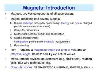
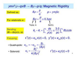
1
Magnet Basics
S. Bernal
USPAS 08
U. of Maryland, College Park
IREAPIREAP
2
Magnets: Introduction
• Magnets are key components of all accelerators
• Magnet modeling has several stages:
1. Simple hardedge models for optics design (energy and type of charged
particle are main considerations)
2. Computer calculations
3. Mechanical/electrical design and construction
4. Magnet measurement:
field/gradient profile and/or multipole measurement
5. Beam testing
• Item 1 requires a magnet strength per amp or volt, and an
effective length. Items 2 and 4 yield actual values.
• Measurement devices: gaussmeters (e.g. Hall-effect), rotating
coils, taut wire techniques, etc.
• Computer codes: OPERA3D/TOSCA, MERMAID, AMPERE, MAG-Li
3
Magnets: Introduction
4
Magnets in UMER: Matching Section
Q2 Solenoid
IC2 IC1
Electron Gun
5
Coordinate Systems and Notation
Bending dipoles define reference trajectory.
6
γγγγmv2/ρρρρ ====qvB → Bρρρρ ====p/q: Magnetic Rigidity
For relativistic e-: 0.3
p
B pc
e
ρ = ≅
Tesla m GeV/c
Bending:
dθ = ds/ρ(s), so
2 2
1 1
2 1
3.0
( )
( )
s s
s s
ds
B s ds
s pc
θ θ
ρ
− = ≅∫ ∫
Focusing: 0x 0yx (z)+ x(z) = 0, y (z)+ y(z) = 0.′′ ′′κ κκ κκ κκ κ
0
0 0
( )
x y
g
B
κ κ
ρ
= − =• Quadrupole:
0r (z)+ r(z) = 0′′ κκκκ• Solenoid:
( )
2
0 2
4
ZB
B
κ
ρ
=
Defined as: ,
p
B
q
ρ = p m cγ β=
7
Magnets: Introduction
Separated Function vs. Combined Function
Electrostatic vs. Magnetostatic
Dipoles, Quadrupoles, Sextupoles, Octupoles
Displaced, overlapping (& infinite) solid elliptical cylinders
carrying uniform current density generate pure fields:
Pure Dipole
+J -J X
Y
BY
X
Pure Quadrupole
Y +J
+J
-J -J
8
UMER PC Dipole and Quadrupole*
Only conductors parallel to z-axis
contribute to integrated B-field.
On a circular cylindrical surface,
we want: ∝∫ ZK dz cosnθ
n=order of multipole. Recall…
-J+J
*W.W. Zhang, et al, Phys, Rev. ST Accel. Beams, 3, 122401 (2000).
UMER PC quadrupole
9
Multipole Expansion
2D Multipole Expansion:
( )
, (1)
 
 
 
 
∑
n-1
x+iy
B(x, y) = B + iB = b +ia ,y x n n rn=1 0
2 2r = x +y < r0
bn = Normal Component,
an = Skew Component
r0 = Aperture Radius
From symmetry, a magnet with quadrupole symmetry has only
multipoles of the form n = 4k+2 (k=0,1,2, …), i.e. quadrupole (n=2),
duodecapole (n=6), 10-pole (n=10), etc.
[ ]
[ ] (2)
 
 
 
 
 
 
∑
∑
n-1
n n
0
n-1
n n
0
r
B (r, θ) = b Sin(nθ)+a Cos(nθ) ,r rn=1
r
B (r, θ) = b Cos(nθ)-a Sin(nθ) .θ rn=1
3D Multipole Expansion:
B → BInt
WE WANT SMALL UNDESIRED MULTIPOLES:
typically less than 1 part in 104
10
UMER Rotating Coil*
The coil contains ~3000
turns of very fine wire.
The whole of the
rotating coil apparatus
is normally enclosed in
mu-metal box.
2nd Gen. UMER
Quadrupole
*W.W. Zhang, et al, Phys, Rev. ST Accel. Beams, 3, 122401 (2000).
11
-80
-70
-60
-50
-40
-30
-20
-10
0
0 10 20 30 40 50 60
FFTofRotatingCoilSignal
(dBm)
Frequency (Hz)
PC QUADRUPOLE
-80
-70
-60
-50
-40
-30
-20
-10
0
0 10 20 30 40 50 60
FFTofRotatingCoilSignal
(dBm)
Frequency (Hz)
PC DIPOLE
-80
-70
-60
-50
-40
-30
-20
-10
0
0 10 20 30 40 50 60
FFTofRotatingCoilSignal
(dBm)
Frequency (Hz)
NO MAGNET
FFT of Rotating Coil Signal
12
UMER Simple Rotating Coil
Rawson-Lush rotating coil gaussmeter
Model 780:
Tip Diameter. A: 6.35 mm
Probe Length B: 50.0 cm
Length to coil center C: 48.9 cm
Tube Diameter E: 6.35 mm
13
Short Solenoid: Axial Field Profile Measurement
For axially symmetric B-fields, components Bz, Br can be found
at all (z, r) from knowledge of Bz(r=0,z)=B(z), i.e. the on-axis field profile:
3 3
3
( , ) ,
2 16
r
r B r B
B r z
z z
∂ ∂
= − + − ⋅⋅⋅
∂ ∂
2 2 4 4
2 4
( , )
4 64
z
r B r B
B r z B
z z
∂ ∂
= − + − ⋅⋅⋅
∂ ∂
14
Review: Modeling of Lenses
′′
δ(z)
x (z)+ x(z) = 0
f
“Point” Lens:
Z
X
f
0 0
1
x (z)+ x(z) = 0 =l
f
′′ →κ κκ κκ κκ κ
Thin Hard-Edge (f>>l):
Zl
X
k0
eff peak
1
x (z)+ (z)x(z) = 0 =l
f
′′ →κ κκ κκ κκ κ
Smooth-Profile:
1
1
z
eff -z
peak
1
l = (z)dzκ
κ ∫
15
Effective Length of UMER Quadrupole*
*S. Bernal, et al, Phys, Rev. ST Accel. Beams, 9, 064202 (2006).
Red curve is analytical fit to
Mag-Li profile (black curve):
g(s)=g0exp(-s2/d2),
g0=3.61 G/cmA, d = 2.10 cm.
0.0
1.0
2.0
3.0
4.0
-10 -7.5 -5 -2.5 0 2.5 5 7.5 10
HE1
HE2
gx
Equation
g(s)(G/cmperAmp)
s (cm)
g0
geff
Standard definition of effective
length (which uses hardtop
gradient g0) yields
leff = 3.72 cm
However, the same focal length can be obtained with a wider
hardedge model with smaller hardtop gradient geff.
For the short UMER quad the correct hardedge model yields
leff = 5.16 cm, geff =0.72×g0
16
Effective Length of Short Solenoid*
For UMER short solenoid, new
treatment yields
leff(cm)= 6.571 cm – 0.00029××××κpeak(m-2),
κeff(m-2)= 0.6945××××κpeak(m-2)
*S. Bernal, et al, Phys, Rev. ST Accel. Beams, 9, 064202 (2006).
UMER Solenoid Profile ( ) ( ) ( )2 2 2
0 0(0, ) exp sech sinhZB z B z d z b C z b = − + 
Similar issues as with the UMER quad…
Effective length calculated the standard
way is leff = 4.50 cm
The effective length has a slight
dependence on peak focusing function.
17
1. K.G. Steffen, High Energy Beam Optics (Wiley, 1965).
2. H. Wiedemann, Particle Accelerator Physics I-II (Springer-Verlag, 1993).
3. P.J. Bryant and K. Johnsen, The Principles of Circular Accelerators and
Storage Rings (Cambridge U. Press, 1993).
4. H. Wolnik, Optics of Charged Particles (Academic Press, 1987).
5. M. Reiser, Theory and Design of Charged-Particle Beams, (Wiley, 1994).
6. USPAS Proceedings (e.g., USPAS 2004).
7. CERN Accelerator School (CAS) Proceedings (e.g., CERN 98-05, CERN
92-05).
8. On-line Journal: Physical Review ST Accel. Beams.
9. Manuals to computer codes like TRANSPORT, TRACE3D, etc.
10. M. Venturini, Ph.D. Thesis (Dept. of Physics, UMCP, 1998).
11. W.W. Zhang, et al, Phys, Rev. ST Accel. Beams, 3, 122401 (2000).
12. S. Bernal, et al, Phys, Rev. ST Accel. Beams, 9, 064202 (2006).
References

Magnet basics

  • 1.
    1 Magnet Basics S. Bernal USPAS08 U. of Maryland, College Park IREAPIREAP
  • 2.
    2 Magnets: Introduction • Magnetsare key components of all accelerators • Magnet modeling has several stages: 1. Simple hardedge models for optics design (energy and type of charged particle are main considerations) 2. Computer calculations 3. Mechanical/electrical design and construction 4. Magnet measurement: field/gradient profile and/or multipole measurement 5. Beam testing • Item 1 requires a magnet strength per amp or volt, and an effective length. Items 2 and 4 yield actual values. • Measurement devices: gaussmeters (e.g. Hall-effect), rotating coils, taut wire techniques, etc. • Computer codes: OPERA3D/TOSCA, MERMAID, AMPERE, MAG-Li
  • 3.
  • 4.
    4 Magnets in UMER:Matching Section Q2 Solenoid IC2 IC1 Electron Gun
  • 5.
    5 Coordinate Systems andNotation Bending dipoles define reference trajectory.
  • 6.
    6 γγγγmv2/ρρρρ ====qvB →Bρρρρ ====p/q: Magnetic Rigidity For relativistic e-: 0.3 p B pc e ρ = ≅ Tesla m GeV/c Bending: dθ = ds/ρ(s), so 2 2 1 1 2 1 3.0 ( ) ( ) s s s s ds B s ds s pc θ θ ρ − = ≅∫ ∫ Focusing: 0x 0yx (z)+ x(z) = 0, y (z)+ y(z) = 0.′′ ′′κ κκ κκ κκ κ 0 0 0 ( ) x y g B κ κ ρ = − =• Quadrupole: 0r (z)+ r(z) = 0′′ κκκκ• Solenoid: ( ) 2 0 2 4 ZB B κ ρ = Defined as: , p B q ρ = p m cγ β=
  • 7.
    7 Magnets: Introduction Separated Functionvs. Combined Function Electrostatic vs. Magnetostatic Dipoles, Quadrupoles, Sextupoles, Octupoles Displaced, overlapping (& infinite) solid elliptical cylinders carrying uniform current density generate pure fields: Pure Dipole +J -J X Y BY X Pure Quadrupole Y +J +J -J -J
  • 8.
    8 UMER PC Dipoleand Quadrupole* Only conductors parallel to z-axis contribute to integrated B-field. On a circular cylindrical surface, we want: ∝∫ ZK dz cosnθ n=order of multipole. Recall… -J+J *W.W. Zhang, et al, Phys, Rev. ST Accel. Beams, 3, 122401 (2000). UMER PC quadrupole
  • 9.
    9 Multipole Expansion 2D MultipoleExpansion: ( ) , (1)         ∑ n-1 x+iy B(x, y) = B + iB = b +ia ,y x n n rn=1 0 2 2r = x +y < r0 bn = Normal Component, an = Skew Component r0 = Aperture Radius From symmetry, a magnet with quadrupole symmetry has only multipoles of the form n = 4k+2 (k=0,1,2, …), i.e. quadrupole (n=2), duodecapole (n=6), 10-pole (n=10), etc. [ ] [ ] (2)             ∑ ∑ n-1 n n 0 n-1 n n 0 r B (r, θ) = b Sin(nθ)+a Cos(nθ) ,r rn=1 r B (r, θ) = b Cos(nθ)-a Sin(nθ) .θ rn=1 3D Multipole Expansion: B → BInt WE WANT SMALL UNDESIRED MULTIPOLES: typically less than 1 part in 104
  • 10.
    10 UMER Rotating Coil* Thecoil contains ~3000 turns of very fine wire. The whole of the rotating coil apparatus is normally enclosed in mu-metal box. 2nd Gen. UMER Quadrupole *W.W. Zhang, et al, Phys, Rev. ST Accel. Beams, 3, 122401 (2000).
  • 11.
    11 -80 -70 -60 -50 -40 -30 -20 -10 0 0 10 2030 40 50 60 FFTofRotatingCoilSignal (dBm) Frequency (Hz) PC QUADRUPOLE -80 -70 -60 -50 -40 -30 -20 -10 0 0 10 20 30 40 50 60 FFTofRotatingCoilSignal (dBm) Frequency (Hz) PC DIPOLE -80 -70 -60 -50 -40 -30 -20 -10 0 0 10 20 30 40 50 60 FFTofRotatingCoilSignal (dBm) Frequency (Hz) NO MAGNET FFT of Rotating Coil Signal
  • 12.
    12 UMER Simple RotatingCoil Rawson-Lush rotating coil gaussmeter Model 780: Tip Diameter. A: 6.35 mm Probe Length B: 50.0 cm Length to coil center C: 48.9 cm Tube Diameter E: 6.35 mm
  • 13.
    13 Short Solenoid: AxialField Profile Measurement For axially symmetric B-fields, components Bz, Br can be found at all (z, r) from knowledge of Bz(r=0,z)=B(z), i.e. the on-axis field profile: 3 3 3 ( , ) , 2 16 r r B r B B r z z z ∂ ∂ = − + − ⋅⋅⋅ ∂ ∂ 2 2 4 4 2 4 ( , ) 4 64 z r B r B B r z B z z ∂ ∂ = − + − ⋅⋅⋅ ∂ ∂
  • 14.
    14 Review: Modeling ofLenses ′′ δ(z) x (z)+ x(z) = 0 f “Point” Lens: Z X f 0 0 1 x (z)+ x(z) = 0 =l f ′′ →κ κκ κκ κκ κ Thin Hard-Edge (f>>l): Zl X k0 eff peak 1 x (z)+ (z)x(z) = 0 =l f ′′ →κ κκ κκ κκ κ Smooth-Profile: 1 1 z eff -z peak 1 l = (z)dzκ κ ∫
  • 15.
    15 Effective Length ofUMER Quadrupole* *S. Bernal, et al, Phys, Rev. ST Accel. Beams, 9, 064202 (2006). Red curve is analytical fit to Mag-Li profile (black curve): g(s)=g0exp(-s2/d2), g0=3.61 G/cmA, d = 2.10 cm. 0.0 1.0 2.0 3.0 4.0 -10 -7.5 -5 -2.5 0 2.5 5 7.5 10 HE1 HE2 gx Equation g(s)(G/cmperAmp) s (cm) g0 geff Standard definition of effective length (which uses hardtop gradient g0) yields leff = 3.72 cm However, the same focal length can be obtained with a wider hardedge model with smaller hardtop gradient geff. For the short UMER quad the correct hardedge model yields leff = 5.16 cm, geff =0.72×g0
  • 16.
    16 Effective Length ofShort Solenoid* For UMER short solenoid, new treatment yields leff(cm)= 6.571 cm – 0.00029××××κpeak(m-2), κeff(m-2)= 0.6945××××κpeak(m-2) *S. Bernal, et al, Phys, Rev. ST Accel. Beams, 9, 064202 (2006). UMER Solenoid Profile ( ) ( ) ( )2 2 2 0 0(0, ) exp sech sinhZB z B z d z b C z b = − +  Similar issues as with the UMER quad… Effective length calculated the standard way is leff = 4.50 cm The effective length has a slight dependence on peak focusing function.
  • 17.
    17 1. K.G. Steffen,High Energy Beam Optics (Wiley, 1965). 2. H. Wiedemann, Particle Accelerator Physics I-II (Springer-Verlag, 1993). 3. P.J. Bryant and K. Johnsen, The Principles of Circular Accelerators and Storage Rings (Cambridge U. Press, 1993). 4. H. Wolnik, Optics of Charged Particles (Academic Press, 1987). 5. M. Reiser, Theory and Design of Charged-Particle Beams, (Wiley, 1994). 6. USPAS Proceedings (e.g., USPAS 2004). 7. CERN Accelerator School (CAS) Proceedings (e.g., CERN 98-05, CERN 92-05). 8. On-line Journal: Physical Review ST Accel. Beams. 9. Manuals to computer codes like TRANSPORT, TRACE3D, etc. 10. M. Venturini, Ph.D. Thesis (Dept. of Physics, UMCP, 1998). 11. W.W. Zhang, et al, Phys, Rev. ST Accel. Beams, 3, 122401 (2000). 12. S. Bernal, et al, Phys, Rev. ST Accel. Beams, 9, 064202 (2006). References