Machine Learning Class Assignment 2
Msc Data Analytics
Trushita Redij
Student ID: 10504099
Dublin Business School
Supervisor: Abhishek Kaushik
Dublin Business School
Assignment Submission Sheet
Msc Data Analytics
Student Name: Trushita Redij
Student ID: 10504099
Programme: Msc Data Analytics
Year: 2019
Supervisor: Abhishek Kaushik
Submission Due Date: 17/12/2019
Project Title: Machine Learning Class Assignment 2
Word Count: 1653
Page Count: 11
Machine Learning Class Assignment 2
Trushita Redij
10504099
Contents
1 Definition 2
1.1 Data Preprocessing . . . . . . . . . . . . . . . . . . . . . . . . . . . . . . 2
1.2 Data Preprocessing Steps . . . . . . . . . . . . . . . . . . . . . . . . . . . 2
1.2.1 Data Quality Assessment . . . . . . . . . . . . . . . . . . . . . . . 3
1.2.2 Feature Aggregation . . . . . . . . . . . . . . . . . . . . . . . . . 3
1.2.3 Feature Sampling . . . . . . . . . . . . . . . . . . . . . . . . . . . 3
1.2.4 Dimensionality Reduction . . . . . . . . . . . . . . . . . . . . . . 3
1.2.5 Feature Encoding . . . . . . . . . . . . . . . . . . . . . . . . . . . 3
2 Definition 4
2.1 Decision tree . . . . . . . . . . . . . . . . . . . . . . . . . . . . . . . . . . 4
2.2 Entropy . . . . . . . . . . . . . . . . . . . . . . . . . . . . . . . . . . . . 5
2.3 Information Gain . . . . . . . . . . . . . . . . . . . . . . . . . . . . . . . 5
3 Chinese Restaurant Algorithm 6
3.0.1 Working . . . . . . . . . . . . . . . . . . . . . . . . . . . . . . . . 7
4 Building Models using Supervised Learning Approach 8
4.1 Data Collection . . . . . . . . . . . . . . . . . . . . . . . . . . . . . . . . 8
4.2 Data Preprocessing . . . . . . . . . . . . . . . . . . . . . . . . . . . . . . 8
4.3 Implementation . . . . . . . . . . . . . . . . . . . . . . . . . . . . . . . . 9
4.3.1 Regression Model . . . . . . . . . . . . . . . . . . . . . . . . . . . 9
4.3.2 Classification Model . . . . . . . . . . . . . . . . . . . . . . . . . 9
1
1 Definition
1.1 Data Preprocessing
Data Preprocessing is a most significant step for Machine Learning. In this step the raw
data is transformed or endcoded so that the machine can parse it for further implement-
ation.
Figure 1: Caption
Raw data has many discrepancies, inconsistency, errors, missing value which needs to
be handled before it is parsed by the machine.
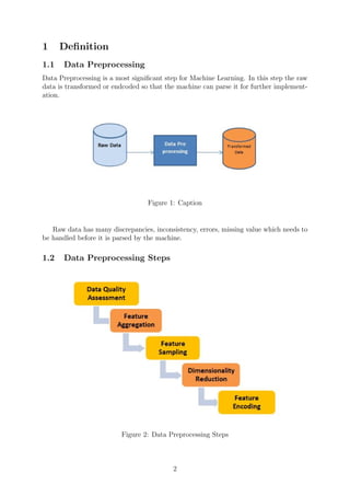
1.2 Data Preprocessing Steps
Figure 2: Data Preprocessing Steps
2
1.2.1 Data Quality Assessment
Raw data is often fetched from multiple sources in different formats thus it becomes
important to structurize the data prior to processing. Various factors are responsible for
data qaulity like human error, measuring devices or redundancy in methods of collecting
data. In this step we primarily focus on enhancing the quality of data by fixing the below
mentioned issues:
1. Missing Value: Eliminating or replacing the missing values. Most common method
used in this scenario is substituting with median,mean or mode value of feature.
2. Inconsistent Value: Dealing with inconsistent data cells wherein it may have merged
the data from another column or split the data. Thus understanding the datatype
of all the variables is necessary
3. Duplicate values: The dataset might contain rows or columns which are duplic-
ated which needs to be removed to avoid bias in implementing machine learning
algorithm.
1.2.2 Feature Aggregation
This step performs aggregation on the feature to derive aggregated values and reduce the
number of objects thereby minimizing consumption of memory and time. Aggregation
helps us build a higher level view of data using groups which are more stable.
1.2.3 Feature Sampling
Sampling it used to derive subset of dataset that we will be analyzing. Sampling algorithm
helps in reducing dataset’s size without reducing the properties of original dataset. This
steps selects the appropriate sampling size and strategy. There are two types of sampling
one with replacement and without replacement.
1.2.4 Dimensionality Reduction
Raw Dataset’s have many features, which needs to be reduced to derive significant output.
Dimensionality reduction is used to reduce the feature size by using feature selection or
subset selection thereby reducing the complexity of dataset.
1.2.5 Feature Encoding
This steps transforms the data to machine readable format. For continues nominal data
one to one mapping is done which helps to retain the meaning of feature. For numeric
variables having intervals or ratios simple mathematical transformation can be used.
3
2 Definition
2.1 Decision tree
In Decision tree learning approach a predictive model is build using observations and
conclusions. Observations about an item are represented in branches and conclusions
about item’s target are represented in leaves (Wik19a).
There are two types of decision tree:
• Classification Tree: These tree models take discrete set of values. Labels are defined
by leaves and concurrence to features are represented by branches.
• Regression Tree: The target variable takes continues set of values.
Figure 3: Decision Tree diagram
The source set is split based on classification features into subsets which comprises of
child node. The process is recursive on derived subset and is called recursive partitioning.
The recursion is concluded when the values in subset matches the target variable. This
top down approach is termed as greedy algorithm
4
2.2 Entropy
Entropy is a measure of the number of ways in which a system may be arranged, often
taken to be a measure of ”disorder” (Wik19c).
In machine learning Entropy can be termed as measure of ambivalence, grime
and confusion.
It establishes control on the splitting of Decision Tree thereby effecting the boundaries
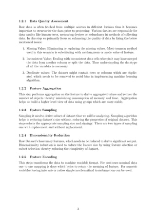
of decision tree. Entropy = -(p(0) * log(P(0)) + p(1) * log(P(1))) Formula for Entropy
is:
Figure 4: Entropy Equation
2.3 Information Gain
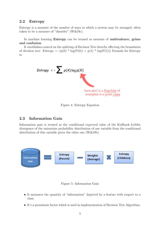
Information gain is termed as the conditional expected value of the Kullback–Leibler
divergence of the univariate probability distribution of one variable from the conditional
distribution of this variable given the other one (Wik19b).
Figure 5: Information Gain
• It measures the quantity of “information” depicted by a feature with respect to a
class.
• It’s a prominent factor which is used in implementation of Decision Tree Algorithm.
5
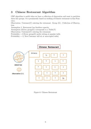
3 Chinese Restaurant Algorithm
CRP algorithm is useful when we have a collection of observation and want to partition
them into groups. It is prominently based on working of Chinese restaurant in San Fran-
cisco.
Observation: Customer(C) entering the restaurant. Group (G) : Collection of Observa-
tion.
Assumption 1: Restaurant has limitless capacity.
Assumption 2:Every group(G) corresponds to a Table(T)
Observation: Customer(C) entering the restaurant.
Probability = 0 Every group(G) prefer sitting at popular table.
Probability = 1( New Customer will sit at unoccupied table)
Figure 6: Chinese Restaurant
6
3.0.1 Working
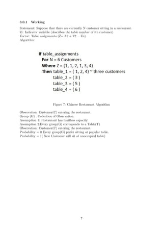
Statement: Suppose that there are currently N customer sitting in a restaurant.
Zi: Indicator variable (describes the table number of ith customer)
Vector: Table assignments (Z= Z1 + Z2.....Zn)
Algorithm:
Figure 7: Chinese Restaurant Algorithm
Observation: Customer(C) entering the restaurant.
Group (G) : Collection of Observation.
Assumption 1: Restaurant has limitless capacity.
Assumption 2:Every group(G) corresponds to a Table(T)
Observation: Customer(C) entering the restaurant.
Probability = 0 Every group(G) prefer sitting at popular table.
Probability = 1( New Customer will sit at unoccupied table)
7
4 Building Models using Supervised Learning Ap-
proach
The proposed dataset highlights All Island Population which includes Northern Ireland
and Republic of Ireland.
4.1 Data Collection
Data Source: https://data.gov.ie/dataset/all-island-population-sa.
This file contains variables from the Population Theme that was produced by AIRO
using data from the census unit at the CSO and the Northern Ireland Research and
Statistics Agency. This data was developed under the Evidence Based Planning theme
of the Ireland Northern Cross Border Cooperation Observatory and CrosSPlaN-2 funded
research programme.
No.Of Rows: 23026
No.of columns: 30
4.2 Data Preprocessing
• Remove null and missing values: The Dataset had no null values or missing
values.
• Convert string type to numeric type The few numeric variables had string
datatype which need to be converted into integer.
• Visualize Dataset Understanding dataset using visualization like histogram, plots,
graphs.
Figure 8: Histogram
• Rescaling Dataset To prepare the data for implementation we used MinMax-
Scaler to rescale the data for effective implementation.
• Plotting Correlation To understand the correlation between the variables and
drop the variables which has highly correlated.
8
The correlation coefficient is an index that ranges from -1 to 1. There exist no
correlation when value is 0.If the value is 1 or -1 it indicates negative correlation.
Figure 9: Correlation Heatmap
4.3 Implementation
4.3.1 Regression Model
We used Linear Regression approach by considering ’Total Population’ as label and ’Fer-
tility rate’ as the dependent variable. We intend to study the effect of fertility rate on
total population of Island which includes Northern Ireland and Republic of Ireland.
Steps:
• Training a Linear Regression Model We assign X array to features and Y array
to target variable that is ’TOTPOP’.
• Train Test Split In order to create model which can be used on new data we
split the datatset into Train data on which we apply linear regression and Test data
wherein we test our algorithm.
• Creating and Training the Model From sklearn.linear model we imported Lin-
ear Regression.
• Predictions from our Model We used the Test dataset to predict our output.
• Visualise the prediction
• Evaluation The mean of the target variable is 277.920304. However the rmse score
on the test data is 123.41 which is lesser then the mean score of target variable.
Thus, using linear model on the given dataset is not efficient.
4.3.2 Classification Model
Steps:
• Training a Linear Regression Model We assign X array to features ’TOT-
POP’,’MALE’,’FEMALE’ and Y array to target variable that is ’Country’.
9
Figure 10: Linear Regression
• Train Test Split In order to create model which can be used on new data we split
the datatset into Train data on which we apply classification and Test data wherein
we test our algorithm.
• Testing accuracy of different classifier We tested accuracy of ’DecisionTree-
Classifier’,’KNeighborsClassifier’, ’GaussianNB’ and ’SVM’.
• Selecting the best fit Classifier and Training the Model We selected KNN
Classifier to train our model as it portrayed highest accuracy on train set as well
as test set.
• Evaluation Confusion matrix, precision, recall and f1 score are the most commonly
used evaluation metrics. The confusion matrix and classification report methods of
the sklearn.metrics were used to evaluate the model.
The KNN algorithm classified all the records in the test set with 80 percent accuracy.
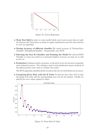
• Comparing Error Rate with the K Value To find the best value of K we plot
the graph of K value and the corresponding error rate for the dataset. Finally, we
plotted the error values against K values
Figure 11: Error Rate K Value
10
References
[Wik19a] Wikipedia contributors, “Decision tree learning — Wikipedia, the free
encyclopedia,” 2019, [Online; accessed 17-December-2019]. [Online]. Avail-
able: https://en.wikipedia.org/w/index.php?title=Decision tree learning&
oldid=926138607
[Wik19b] ——, “Information gain in decision trees — Wikipedia, the free
encyclopedia,” 2019, [Online; accessed 18-December-2019]. [Online].
Available: https://en.wikipedia.org/w/index.php?title=Information gain in
decision trees&oldid=930926162
[Wik19c] ——, “Introduction to entropy — Wikipedia, the free encyclopedia,”
2019, [Online; accessed 18-December-2019]. [Online]. Available: https://en.
wikipedia.org/w/index.php?title=Introduction to entropy&oldid=926007171
11

Machine_Learning_Trushita

  • 1.
    Machine Learning ClassAssignment 2 Msc Data Analytics Trushita Redij Student ID: 10504099 Dublin Business School Supervisor: Abhishek Kaushik
  • 2.
    Dublin Business School AssignmentSubmission Sheet Msc Data Analytics Student Name: Trushita Redij Student ID: 10504099 Programme: Msc Data Analytics Year: 2019 Supervisor: Abhishek Kaushik Submission Due Date: 17/12/2019 Project Title: Machine Learning Class Assignment 2 Word Count: 1653 Page Count: 11
  • 3.
    Machine Learning ClassAssignment 2 Trushita Redij 10504099 Contents 1 Definition 2 1.1 Data Preprocessing . . . . . . . . . . . . . . . . . . . . . . . . . . . . . . 2 1.2 Data Preprocessing Steps . . . . . . . . . . . . . . . . . . . . . . . . . . . 2 1.2.1 Data Quality Assessment . . . . . . . . . . . . . . . . . . . . . . . 3 1.2.2 Feature Aggregation . . . . . . . . . . . . . . . . . . . . . . . . . 3 1.2.3 Feature Sampling . . . . . . . . . . . . . . . . . . . . . . . . . . . 3 1.2.4 Dimensionality Reduction . . . . . . . . . . . . . . . . . . . . . . 3 1.2.5 Feature Encoding . . . . . . . . . . . . . . . . . . . . . . . . . . . 3 2 Definition 4 2.1 Decision tree . . . . . . . . . . . . . . . . . . . . . . . . . . . . . . . . . . 4 2.2 Entropy . . . . . . . . . . . . . . . . . . . . . . . . . . . . . . . . . . . . 5 2.3 Information Gain . . . . . . . . . . . . . . . . . . . . . . . . . . . . . . . 5 3 Chinese Restaurant Algorithm 6 3.0.1 Working . . . . . . . . . . . . . . . . . . . . . . . . . . . . . . . . 7 4 Building Models using Supervised Learning Approach 8 4.1 Data Collection . . . . . . . . . . . . . . . . . . . . . . . . . . . . . . . . 8 4.2 Data Preprocessing . . . . . . . . . . . . . . . . . . . . . . . . . . . . . . 8 4.3 Implementation . . . . . . . . . . . . . . . . . . . . . . . . . . . . . . . . 9 4.3.1 Regression Model . . . . . . . . . . . . . . . . . . . . . . . . . . . 9 4.3.2 Classification Model . . . . . . . . . . . . . . . . . . . . . . . . . 9 1
  • 4.
    1 Definition 1.1 DataPreprocessing Data Preprocessing is a most significant step for Machine Learning. In this step the raw data is transformed or endcoded so that the machine can parse it for further implement- ation. Figure 1: Caption Raw data has many discrepancies, inconsistency, errors, missing value which needs to be handled before it is parsed by the machine. 1.2 Data Preprocessing Steps Figure 2: Data Preprocessing Steps 2
  • 5.
    1.2.1 Data QualityAssessment Raw data is often fetched from multiple sources in different formats thus it becomes important to structurize the data prior to processing. Various factors are responsible for data qaulity like human error, measuring devices or redundancy in methods of collecting data. In this step we primarily focus on enhancing the quality of data by fixing the below mentioned issues: 1. Missing Value: Eliminating or replacing the missing values. Most common method used in this scenario is substituting with median,mean or mode value of feature. 2. Inconsistent Value: Dealing with inconsistent data cells wherein it may have merged the data from another column or split the data. Thus understanding the datatype of all the variables is necessary 3. Duplicate values: The dataset might contain rows or columns which are duplic- ated which needs to be removed to avoid bias in implementing machine learning algorithm. 1.2.2 Feature Aggregation This step performs aggregation on the feature to derive aggregated values and reduce the number of objects thereby minimizing consumption of memory and time. Aggregation helps us build a higher level view of data using groups which are more stable. 1.2.3 Feature Sampling Sampling it used to derive subset of dataset that we will be analyzing. Sampling algorithm helps in reducing dataset’s size without reducing the properties of original dataset. This steps selects the appropriate sampling size and strategy. There are two types of sampling one with replacement and without replacement. 1.2.4 Dimensionality Reduction Raw Dataset’s have many features, which needs to be reduced to derive significant output. Dimensionality reduction is used to reduce the feature size by using feature selection or subset selection thereby reducing the complexity of dataset. 1.2.5 Feature Encoding This steps transforms the data to machine readable format. For continues nominal data one to one mapping is done which helps to retain the meaning of feature. For numeric variables having intervals or ratios simple mathematical transformation can be used. 3
  • 6.
    2 Definition 2.1 Decisiontree In Decision tree learning approach a predictive model is build using observations and conclusions. Observations about an item are represented in branches and conclusions about item’s target are represented in leaves (Wik19a). There are two types of decision tree: • Classification Tree: These tree models take discrete set of values. Labels are defined by leaves and concurrence to features are represented by branches. • Regression Tree: The target variable takes continues set of values. Figure 3: Decision Tree diagram The source set is split based on classification features into subsets which comprises of child node. The process is recursive on derived subset and is called recursive partitioning. The recursion is concluded when the values in subset matches the target variable. This top down approach is termed as greedy algorithm 4
  • 7.
    2.2 Entropy Entropy isa measure of the number of ways in which a system may be arranged, often taken to be a measure of ”disorder” (Wik19c). In machine learning Entropy can be termed as measure of ambivalence, grime and confusion. It establishes control on the splitting of Decision Tree thereby effecting the boundaries of decision tree. Entropy = -(p(0) * log(P(0)) + p(1) * log(P(1))) Formula for Entropy is: Figure 4: Entropy Equation 2.3 Information Gain Information gain is termed as the conditional expected value of the Kullback–Leibler divergence of the univariate probability distribution of one variable from the conditional distribution of this variable given the other one (Wik19b). Figure 5: Information Gain • It measures the quantity of “information” depicted by a feature with respect to a class. • It’s a prominent factor which is used in implementation of Decision Tree Algorithm. 5
  • 8.
    3 Chinese RestaurantAlgorithm CRP algorithm is useful when we have a collection of observation and want to partition them into groups. It is prominently based on working of Chinese restaurant in San Fran- cisco. Observation: Customer(C) entering the restaurant. Group (G) : Collection of Observa- tion. Assumption 1: Restaurant has limitless capacity. Assumption 2:Every group(G) corresponds to a Table(T) Observation: Customer(C) entering the restaurant. Probability = 0 Every group(G) prefer sitting at popular table. Probability = 1( New Customer will sit at unoccupied table) Figure 6: Chinese Restaurant 6
  • 9.
    3.0.1 Working Statement: Supposethat there are currently N customer sitting in a restaurant. Zi: Indicator variable (describes the table number of ith customer) Vector: Table assignments (Z= Z1 + Z2.....Zn) Algorithm: Figure 7: Chinese Restaurant Algorithm Observation: Customer(C) entering the restaurant. Group (G) : Collection of Observation. Assumption 1: Restaurant has limitless capacity. Assumption 2:Every group(G) corresponds to a Table(T) Observation: Customer(C) entering the restaurant. Probability = 0 Every group(G) prefer sitting at popular table. Probability = 1( New Customer will sit at unoccupied table) 7
  • 10.
    4 Building Modelsusing Supervised Learning Ap- proach The proposed dataset highlights All Island Population which includes Northern Ireland and Republic of Ireland. 4.1 Data Collection Data Source: https://data.gov.ie/dataset/all-island-population-sa. This file contains variables from the Population Theme that was produced by AIRO using data from the census unit at the CSO and the Northern Ireland Research and Statistics Agency. This data was developed under the Evidence Based Planning theme of the Ireland Northern Cross Border Cooperation Observatory and CrosSPlaN-2 funded research programme. No.Of Rows: 23026 No.of columns: 30 4.2 Data Preprocessing • Remove null and missing values: The Dataset had no null values or missing values. • Convert string type to numeric type The few numeric variables had string datatype which need to be converted into integer. • Visualize Dataset Understanding dataset using visualization like histogram, plots, graphs. Figure 8: Histogram • Rescaling Dataset To prepare the data for implementation we used MinMax- Scaler to rescale the data for effective implementation. • Plotting Correlation To understand the correlation between the variables and drop the variables which has highly correlated. 8
  • 11.
    The correlation coefficientis an index that ranges from -1 to 1. There exist no correlation when value is 0.If the value is 1 or -1 it indicates negative correlation. Figure 9: Correlation Heatmap 4.3 Implementation 4.3.1 Regression Model We used Linear Regression approach by considering ’Total Population’ as label and ’Fer- tility rate’ as the dependent variable. We intend to study the effect of fertility rate on total population of Island which includes Northern Ireland and Republic of Ireland. Steps: • Training a Linear Regression Model We assign X array to features and Y array to target variable that is ’TOTPOP’. • Train Test Split In order to create model which can be used on new data we split the datatset into Train data on which we apply linear regression and Test data wherein we test our algorithm. • Creating and Training the Model From sklearn.linear model we imported Lin- ear Regression. • Predictions from our Model We used the Test dataset to predict our output. • Visualise the prediction • Evaluation The mean of the target variable is 277.920304. However the rmse score on the test data is 123.41 which is lesser then the mean score of target variable. Thus, using linear model on the given dataset is not efficient. 4.3.2 Classification Model Steps: • Training a Linear Regression Model We assign X array to features ’TOT- POP’,’MALE’,’FEMALE’ and Y array to target variable that is ’Country’. 9
  • 12.
    Figure 10: LinearRegression • Train Test Split In order to create model which can be used on new data we split the datatset into Train data on which we apply classification and Test data wherein we test our algorithm. • Testing accuracy of different classifier We tested accuracy of ’DecisionTree- Classifier’,’KNeighborsClassifier’, ’GaussianNB’ and ’SVM’. • Selecting the best fit Classifier and Training the Model We selected KNN Classifier to train our model as it portrayed highest accuracy on train set as well as test set. • Evaluation Confusion matrix, precision, recall and f1 score are the most commonly used evaluation metrics. The confusion matrix and classification report methods of the sklearn.metrics were used to evaluate the model. The KNN algorithm classified all the records in the test set with 80 percent accuracy. • Comparing Error Rate with the K Value To find the best value of K we plot the graph of K value and the corresponding error rate for the dataset. Finally, we plotted the error values against K values Figure 11: Error Rate K Value 10
  • 13.
    References [Wik19a] Wikipedia contributors,“Decision tree learning — Wikipedia, the free encyclopedia,” 2019, [Online; accessed 17-December-2019]. [Online]. Avail- able: https://en.wikipedia.org/w/index.php?title=Decision tree learning& oldid=926138607 [Wik19b] ——, “Information gain in decision trees — Wikipedia, the free encyclopedia,” 2019, [Online; accessed 18-December-2019]. [Online]. Available: https://en.wikipedia.org/w/index.php?title=Information gain in decision trees&oldid=930926162 [Wik19c] ——, “Introduction to entropy — Wikipedia, the free encyclopedia,” 2019, [Online; accessed 18-December-2019]. [Online]. Available: https://en. wikipedia.org/w/index.php?title=Introduction to entropy&oldid=926007171 11