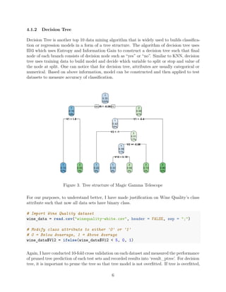
The document compares the performance of four common data mining algorithms (KNN, decision trees, EM, and k-means clustering) across three datasets. It describes the datasets, experimental procedure using 10-fold cross-validation, and provides the results of applying each algorithm to each dataset. The key finding is that the algorithm performance varies significantly depending on the characteristics of the particular dataset, with decision trees achieving the highest accuracy on the wine quality dataset while k-means performed best on the spam dataset. The conclusion is that the suitability of algorithms depends heavily on the domain and properties of the data.

1. Comparison of Top Data Mining
Algorithms
Jimmy Sanghun Kim
December 12, 2016
Contents
1 Introduction 2
2 Acknowledgement 2
3 Experimental Procedure 2
3.1 Dataset Descriptions . . . . . . . . . . . . . . . . . . . . . . . . . . . . . . . 3
3.1.1 Wine Quality . . . . . . . . . . . . . . . . . . . . . . . . . . . . . . . 3
3.1.2 Magic Gamma Telescope . . . . . . . . . . . . . . . . . . . . . . . . . 4
3.1.3 Spambase . . . . . . . . . . . . . . . . . . . . . . . . . . . . . . . . . 4
4 Algorithms 4
4.1 Classification . . . . . . . . . . . . . . . . . . . . . . . . . . . . . . . . . . . 4
4.1.1 K-Nearest Neighbor(KNN) . . . . . . . . . . . . . . . . . . . . . . . . 4
4.1.2 Decision Tree . . . . . . . . . . . . . . . . . . . . . . . . . . . . . . . 6
4.2 Clustering . . . . . . . . . . . . . . . . . . . . . . . . . . . . . . . . . . . . . 8
4.2.1 Expectation Maximization(EM) . . . . . . . . . . . . . . . . . . . . . 8
4.2.2 K-Means . . . . . . . . . . . . . . . . . . . . . . . . . . . . . . . . . . 9
5 Implication 11
6 Conclusion 11
7 Reference 12
1

2. 1 Introduction
In recent past, data mining has become one of the fastest growing and essential professional
field as there has been tremendous amount of data that needs to be processed and analyzed
in effective ways to make meaningful decisions. Algorithms varies in accuracy based on
the domains, shape, labels of data and etc. Thus the goal of our research is to investigate
how top data mining algorithms such as K-Nearest Neighbor, Decision Tree, Expectation
Maximization and K-means perform in different datasets using R.
2 Acknowledgement
First and foremost, I would like to thank my mentor Hasan Kurban, Ph D. candidate in the
School of Informatics and Computing at Indiana University Bloomington. My first contact
with Hasan was through Undergraduate Research Opportunities in Computing(UROC) at
Indiana University. Since then, he, as a mentor, provided me with valuable guidance, strong
support and encouraged me throughout the entire program. In addition, I would like to
thank Lamara D.Warren, Interim Assistant Dean for Diversity and Education at School of
Informatics and Computing for giving me opportunity in UROC and have great experience
3 Experimental Procedure
The datasets chosen for the analysis has been downloaded from UCI Machine Learning
Repository and also provided by mentor. The datasets descriptions are available in next
section and they are:
• Wine Quality(White)
• Magic Gamma Telescope
• Spambase
For each dataset, two classification and two clustering algorithms will be applied to observe
performances of each algorithm on different datasets. Those algorithms are:
• Classification
– K-Nearest Neighbor(KNN)
– Decision Tree
• Clustering
– Expectation Maximization
– K-Means
2

3. Figure 1. Procedure
3.1 Dataset Descriptions
In data mining, understanding domain of dataset is crucial in order to obtain specific
information we look for in the data. Each dataset has its own unique attributes, characteristics,
labels and shapes such that performances of each algorithms can vary accordingly. Below
table 1 summarizes the dataset we are going to use in the experiments.
Dataset No.of attributes Classes No.of records
Wine Quality 12 7 4898
Magic Gamma Telescope 11 2 19021
Spambase 58 2 4602
3.1.1 Wine Quality
Wine quality dataset is about variants of the Portuguese “Vinho Verde”" wine. The inputs
include 12 features (e.g. PH values) and 1 of them refers to the output which is based on
sensory data (median of at least 3 evaluations made by wine experts). Each expert graded
the wine quality between 0 (very bad) and 10 (very excellent). There are 4898 records and 7
classes without any missing values.
3

4. 3.1.2 Magic Gamma Telescope
This dataset consist of 11 features and 1 of them being class attribute which is either ‘g’ or
‘h’ but for our purpose, classes have been changed into ‘1’ or ‘2’. Among all datasets, Magic
Gamma Telescope dataset has most observation of 19021. With similar number of attributes
compared to ‘Wine Quality’ dataset, we can compare how classes and number of records can
have effect on performance.
3.1.3 Spambase
Spambase has most number of attributes which is 58 and one of them also refers to class
attribute. Similarly, the class attribute consists of either ‘0’ or ‘1’ which denotes whether the
e-mail was considered as spam or not.
4 Algorithms
4.1 Classification
Classification, a supervised learning method is one of the most widely used data mining
technique which uses labeled data. Classification predicts a certain outcome (class) based on
a given input (features). In order to predict the outcome, algorithm processes a training set
containing a set of attributes and the respective outcome (class) thereby understanding a
relationship between features which makes possible to predict outcome when test set is given
without respective outcome.
4.1.1 K-Nearest Neighbor(KNN)
K-Nearest Neighbor, one of the top data mining algorithm, is a non-parametric lazy learning
algorithm which means predicting an outcome of test set is heavily based on the training
phase. It finds a group of k data points in the training set that are closest to the test object
and assigns a label based on majority of particular class in the neighborhood.
Let’s take a look at how KNN classification is done with Wine Quality data set.
# Perform 10 fold cross validation
folds <- cut(seq(1, nrow(norm_wine)), breaks=10, labels=FALSE)
# KNN with k=5
for (i in 1:10) {
testIndex <- which(folds==i, arr.ind=TRUE)
test_data = norm_wine[testIndex, ]
training_data = norm_wine[-testIndex, ]
4

5. test_target = wine_cls[testIndex]
training_target = wine_cls[-testIndex]
# KNN takes place here!
require(class)
pred = knn(train=training_data, test=test_data, cl=training_target, k=5)
result_wine[i] = mean(test_target != pred)
}
Above example takes k=5 and performs 10 fold cross validation to observe the accuracy
of KNN classification. In each fold, dataset is divided into training and test set and KNN
calculates distance of each data points in the neighborhood. Then selecting 5 nearest
neighborhood data points, assigns class that is dominant to the test set label. This pro-
cess will be repeated on different number of k and datasets. The results are as follows:
k5 k9 k13 k17 k21 k25
Accuracy of K−Nearest Neighbor with different K in each data sets
Number of K
Percentage
020406080100
Wine Quality
Magic
Spam
Figure 2.
5

6. 4.1.2 Decision Tree
Decision Tree is another top 10 data mining algorithm that is widely used to builds classifica-
tion or regression models in a form of a tree structure. The algorithm of decision tree uses
ID3 which uses Entropy and Information Gain to construct a decision tree such that final
node of each branch consists of decision node such as “yes” or “no”. Similar to KNN, decision
tree uses training data to build model and decide which variable to split or stop and value of
the node at split. One can notice that for decision tree, attributes are usually categorical or
numerical. Based on above information, model can be constructed and then applied to test
datasets to measure accuracy of classification.
Figure 3. Tree structure of Magic Gamma Telescope
For our purposes, to understand better, I have made justification on Wine Quality’s class
attribute such that now all data sets have binary class.
# Import Wine Quality dataset
wine_data = read.csv("winequality-white.csv", header = FALSE, sep = ";")
# Modify class attribute to either '0' or '1'
# 0 = Below Avaerage, 1 = Above Average
wine_data$V12 = ifelse(wine_data$V12 < 5, 0, 1)
Again, I have conducted 10-fold cross validation on each dataset and measured the performance
of pruned tree prediction of each test sets and recorded results into ‘result_ptree’. For decision
tree, it is important to prune the tree so that tree model is not overfitted. If tree is overfitted,
6

7. it would mean that the branch has not much use in predicting class for test sets but still
taking up the space which increases runtime decreasing efficiency.
result_ptree = vector("numeric", 10)
for (i in 1:10) {
testIndex <- which(folds==i, arr.ind=TRUE)
test_data = spam_data[testIndex, -c(58)]
training_data = spam_data[-testIndex, ]
test_target = spam_data[testIndex, c(58)]
training_target = spam_data[-testIndex, c(58)]
dtree_model = rpart(training_data$X.V58.~.,
data=training_data, method = "class")
ptree_model = prune(dtree_model, cp= dtree_model$cptable...
[which.min(dtree_model$cptable[,"xerror"]),"CP"])
ptree_pred = predict(ptree_model, test_data, type = "class")
result_ptree[i]= mean(ptree_pred != test_target)
}
Wine Quality Magic Spam
Accuracy of Decision Tree in each data sets
Data sets
Percentages
020406080100
Wine Quality
Magic
Spam
Figure 4.
7

8. 4.2 Clustering
Clustering, unsupervised learning method which groups a set of objects in a way that objects
in the same group(cluster) has similar characteristics among each other than those in other
groups. During clustering, data points are partitioned into set of data based on their similarity
and then assign label according to the cluster they are in. This label does not necesarily
corresponds to actual label, if exists, because in real world, there are a lot of data without
labels and clustering is to help distinguish and discover distinct patterns out of dataset.
Overall, I believe clustering is great tool to observe the behavior and characteristics of clusters
in datasets.
4.2.1 Expectation Maximization(EM)
Expectation Maximization(EM) is parametric and iterative method for finding maximum
liklihood of parameters. EM algorithm requires a probability distribution. In this research, I
have used R package called ‘Mclust’ which builds cluster model for parameterized Gaussian
mixture models. There are two steps in EM algorithm which is E-step and M-step. In E-step,
also known as expectation step, creates function for the expectation of the log-likelihood
calcualted from the current estimate for the parameters. For M-step, it computes parameters
maximizing the expected log-liklihood found in E-step.
To calculate the accuracy of how well each data set is clustered, I have first built a model
based on the half of dataset as training set and applied the other half of data set as test set
and predicted how well test set fall into cluster based on model built with training set. Below
shows code for wine quality dataset and followed by result.
#Clustering
require(mclust)
folds <- cut(seq(1, nrow(wine_data)), breaks=2, labels=FALSE)
result_wine = vector("numeric", 2)
for (i in 1:2) {
testIndex <- which(folds==i, arr.ind=TRUE)
test_data = wine_data[testIndex, ]
training_data = wine_data[-testIndex, ]
mod = Mclust(training_data, G= 7)
em_pred = predict.Mclust(mod, test_data)
print(table(mod$classification))
print(table(em_pred$classification))
result_wine[i] = mean(em_pred$classification != mod$classification)
}
8

9. Wine Quality Magic Spam
Accuracy of EM Model in each data sets
Data sets
Percentages
020406080100
Wine Quality
Magic
Spam
Figure 5.Result of Expectation-Maximization(EM)
4.2.2 K-Means
K-Means is a hard clustering algorithm that takes k, number of cluster, and assgins all of
the datapoints within those cluster specified by user. First step for K-means is to randomly
choose cluster center c then calculate the distance between each data points to the cluster
centers c. After that, it assigns data points to the cluster whose distance is shortest of all
cluster centers. These processes will be iteratively repeated with new random cluster centers
chosen from datapoint in each cluster until convergence, convergence is when all data points
stop shifting clusters(reassignment).
folds <- cut(seq(1, nrow(spam_data)), breaks=2, labels=FALSE)
result_spam = vector("numeric", 2)
for (i in 1:2) {
testIndex <- which(folds==i, arr.ind=TRUE)
test_data = spam_data[testIndex, ]
test_data = test_data[1:2300, ]
training_data = spam_data[-testIndex, ]
training_data = training_data[1:2300, ]
9

10. km_mod = kmeans(training_data, 2)
km_pred = cl_predict(km_mod, test_data, type = "class_ids")
result_spam[i] = mean(km_pred != km_mod$cluster)
}
Wine Quality Magic Spam
Accuracy of Kmeans in each data sets
Data sets
Percentages
020406080100
Wine Quality
Magic
Spam
Figure 6. Result of K-means
10

11. 5 Implication
Figure 7. Results of each algorithm on different set of data
I have applied two clustering and two classification algorithms to ‘Wine Quality’, ‘MagicGam-
maTelescope’ and ‘Spambase’ data sets. Implying from results, as we assumed, accuracy
in each datasets varies. For ‘Wine Quality’, accuracy was highest in Decision Tree whereas
lowest in all other algorithms. ‘MagicGammaTelescope’ and ‘Spambase’ datasets have fairly
high accuracy in classification algorithms but fairly low in clustering except that ‘Spambase’
had high accuracy in Kmeans. For EM, overall performances were low compare to other
algorithms such that shape of each dataset may have been different from multivariate gaussian
distribution which EM use to cluster.
6 Conclusion
The goal of our research was to compare the performances of each top data mining algorithm
on different datasets. We can conclude that characteristics of datasets can influence the
accuracy and it is crucial to understand domains of data and preprocess in data cleaning
stage. There are no specific algorithm assigned to datasets as there are many possible ways
to measure high accuracy in data mining field.
11

12. 7 Reference
• UCI Machine Learning Repository
• Top 10 algorithms in data mining
12