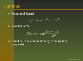
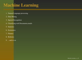
Machine Learning
Supervised Learning and Support Vector Machine
                         Raj Kamal
                   r.kamal@iitg.ernet.in


                 Department of Mathematics
           Indian Institute of Technology,Guwahati
                   Guwahati-781039,India


                                                     Machine Learning – p. 1
Seminar
          1-1
Outline of the talk
    Introduction


                      Machine Learning – p. 2
Outline of the talk
    Introduction
    Motivation


                      Machine Learning – p. 2
Outline of the talk
    Introduction
    Motivation
    Support Vector Machines


                              Machine Learning – p. 2
Outline of the talk
    Introduction
    Motivation
    Support Vector Machines
    Softwares


                              Machine Learning – p. 2
Outline of the talk
    Introduction
    Motivation
    Support Vector Machines
    Softwares
    Applications


                              Machine Learning – p. 2
Outline of the talk
    Introduction
    Motivation
    Support Vector Machines
    Softwares
    Applications
    Conclusion


                              Machine Learning – p. 2
Outline of the talk
    Introduction
    Motivation
    Support Vector Machines
    Softwares
    Applications
    Conclusion


                              Machine Learning – p. 2
Machine Learning
  Machine learning, a branch of artificial intelligence, is a scientific discipline concerned with the
  design and development of algorithms that allow computers to evolve behaviors based on
  empirical data, such as from sensor data or databases.
  Here computer learns the algorithms from the experience.
  Idea: Synthesize computer programs by learning from representative examples of input (and
  output) data. Rationale Learning from Examples: A. For many problems, there is no known
  method for computing the desired output from a set of inputs. B. For other problems, computation
  according to the known correct method may be too expensive.
  How can we build computer systems that automatically improve with experience, and what are the
  fundamental laws that govern all learning processes?
  Machine Learning


                                                                                           Machine Learning – p. 3
continue
   What is the Learning Problem?
   Learning = Improving with experience at some task
   1. Improve over task T ,
   2. with respect to performance measure P
   3. based on experience E


                                               Machine Learning – p. 4
continue
   What is the Learning Problem?
   Learning = Improving with experience at some task
   1. Improve over task T ,
   2. with respect to performance measure P
   3. based on experience E


                                               Machine Learning – p. 4
Variants of Machine Learning
 1. Supervised Learning : Given a set of label training-data xi, yi , with xi be a set of samples and yi a
    set of labels.
 2. Unsupervised Learning : Given only a set of data xi . Learning without output values (data
    exploration, e.g. clustering).
 3. Query Learning : Learning where the learner can query the environment about the output
    associated with a particular input.
 4. Reinforcement Learning : Learning where the learner has a range of actions which it can take to
    attempt to move towards states where it can expect high rewards. Cocktail Party Problem ,Sound
    overlapping and verification
Problems are solved using methods of statistics: Regression,EM algorithm,MLE algorithm


                                                                                               Machine Learning – p. 5
Supervised Learning
 1. Training Set :- Training Examples where input and output are known from experiment
 2. x(i) :- ith Input value/vector
 3. y (i) :- ith Output value/vector
 4. (x(i) ,y (i) ) i=1...m:- Training set,m input and output training examples
 5. X :- space of input value/vector
 6. Y :- space of output value/vector.
 7. To describe the supervised learning problem,our goal is to learn a function h(x) : X → Y . such
    that h(x) is a good predictor of corresponding value of y.
 8. h(x) :- hypothesis


                                                                                          Machine Learning – p. 6
Continue
 1. When Target Domain is continuos we call learning problem a Regression Problem.
 2. When Y can take descrete value we call it as Classification Problem
 3. x ∈ ā„œn ,n= no. of features
 4. xi :- jth feature of ith training set.
     j

 5. an ith training set can have different features (shapes,size,cost).
 6. To perform Supervised Learning,we must decide how we are going to do .
 7. hā„œĪø = Īø0 + Īø1 āˆ— x1 + ... + Īøn āˆ— xn .
 8. hĪø (x) = Σθi āˆ— xi where x0 = 1
 9. classifier =0,1


                                                                                     Machine Learning – p. 7
Support Vector Machine(SVM)
 Most classification tasks are not as simple ,more complex structure are needed to make optimal
   separation,full separation would require a curve


 We can see the original objects mapped i.e, rearranged using a set of mathematical functions called
   kernels.By this they are linearly separable
 Instead of constructing the complex curve all we have to do is to find a optimal line that can separate
    these as positive and negative examples
 SVM is primarily a classifier method that performs classification task by cosntructing
 Goal : To optimize decision boundary.

                                                                                             Machine Learning – p. 8
continue


  Binary classifier :-Y Ē«āˆ’1, 1

                                Machine Learning – p. 9
continue
  Y Ē«āˆ’1, 1
  hω,b (x) = g(ω T x + b)
  Īøi are repalced with ωi
  g(z) = 1, z ≄ 0
  g(z) = 0, otherwise
  ω = (ω1 , ω2 , ....., ωn )T


                                Machine Learning – p. 10
continue
  Functional Margin:
     Given (x(i) , y (i0 ) ith training set we define Functional Margin
     ˆ
     Ī„(i) = y (i) (ω (T ) x + b)
     y (i) = āˆ’1 functional margin to be large we need (ω T x + b) to be large (more negative)
     y (i) = 1 functional margin to be large we need (ω T x + b) to be large (more positive)
     functional margin large,so that our predictio is correct and confident.
     Although it is not a good measure (scaling can have adverse effect ,it scales up just by
     exploiting the scaling freedom and make functional margin large )
     Functional Margin:
     Ī„ = min(΄ˆ )i = 1, 2, 3, ...m.
     ˆ           (i)


                                                                                          Machine Learning – p. 11
continue


   Geometric Margin
     decision boundary corresponding to (ω,b)
     distance of A from decision boundary =AB Ī„(i)
       (ω)
      ( ω )   unit vector pointing in same direction as ω

                       i     i    ω
                      x āˆ’Ī„ āˆ—           →B
                                  ω                 Machine Learning – p. 12
continue
 the above satisfy ω T āˆ— x + b = 0
 solving :- γ (i) = (     ω
                          ω     āˆ— x(i) +   b
                                           ω   )
 Geometrical Margin :

                  (i)         (i)      ω               b
              γ         =y          āˆ—(   ) āˆ— x(i) +
                                       ω               ω
 It is invariant to scaling.

                        γ = min(γ (i) ), i = 1, 2..m


                                                           Machine Learning – p. 13
continue
   OPTIMAL MARGIN CLASSIFIER
   Given a Training set,it seems from previous natural
   desideration is to find decision
   boundary that optimizes the geometric margin,since
   this would reject a very confident set of
   prediction on the training set and a good fit to train
   data.
   Classifier that separates positive and negative
   training examples with gap.


                                                  Machine Learning – p. 14
continue
  This lead to the following Optimization Problem
  max΄ωb Ī„i = 1, 2, .., m
                                  ˆ
  such that y (i) ((ω)T xi + b) ≄ Ī„i = 1, 2, ...m
    ω 2 = 1 Functional Margin = Geometric Margin
  Functional margin at least Ī„ and we maximise Geometric margin.
              ˆ
              Ī„
  max΄ωb     ω 2
  such thaty (i) ((ω)T xi          ˆ
                            + b) ≄ Ī„i = 1, 2, ...m
          ˆ
  impose Ī„ = 1
  minĪ„,ω,b 1 ω 2
              2
  such that y (i) ((ω)T xi + b) ≄ 1i = 1, 2, ...m


  The following gives optimal Margin Classifier ,we can solve by QP quadratic programming Code.


                                                                                    Machine Learning – p. 15
continue
  gi (ω) = āˆ’y i (ω T xi + b) + 1
  Āø
  OPtical Margin Classifiers
  minĪ„,ω,b 1 ω 2
              2
  such that gi (ω) ≤ 0
            Āø
  Dual
  maxαW (α) = Σαi āˆ’ 1 Ī£y (i) y (j) αi αj < x(i) , x(j) > αi ≄ 0, i = 1, 2, ...m
                            2
  Σαi y (i) = 0i = 1, 2, , ...m


                                                                                  Machine Learning – p. 16
continue
  on Solving we get


                                          ω = Σαi y (i) x(i)


                        max( i : y (i) = āˆ’1)ω T X (i) + min( i : y (i) = 1)ω T X (i)
                b=
                                                     2
                      f (x) = ω T X + b = Ī£( i = 1, 2, ..m)αi y (i) < xi , x > +b

                                       hω,b (x) = g(ω T x + b)


                                                                                       Machine Learning – p. 17
continue
  What if Data set is too hard to linearly separate
  We add slack variables ξ to allow misclassification of difficult noise reults called Soft Margin


  Primal

                                          1
                                  minγ,ω,b ( ω )2 + CĪ£m ξi
                                                      i=1
                                          2
  such that
                            y (i) (ω T āˆ— x(i) + b) ≄ 1 āˆ’ ξi i = 1, 2, ..., m
                                                ξi ≄ 0
  ,i=1,2,..m
  now we have permitted to chose functional margin less than 1

                                                C[Σξi
  controls                                                                                Machine Learning – p. 18
continue
  What if the data set is too hard to handle ,then we map input to higher dimentional using kernels
  φ(x) : x → Ļ•(x)
  φ(x)=feature mapping which maps attribute to input features
  K(x, z) = φ(x)T φ(x)
  replace
                                       < x, z > withK(x, z)

  exploit it to use SVM implicitely to slove
  Kernels
  polynomial kernel ,Guassian kernel


                                                                                          Machine Learning – p. 19
continue


  Polynomial kernel

                                        
                                 x1 x1
                                    
                              x1 x2 
                                    
                                    
                              x1 x3 
                                    
                                    
                              x2 x1 
                                    
                              x2 x2 
                                    
                                    
                             x x 
                              2 3 
                                    
                      φ(x) = 
                              x3 x1 
                                     
                                    
                              x3 x2 
                                    
                                    
                              x3 x3 
                             √      
                              2cx1 
                                           Machine Learning – p. 20
                                    
continue
   Polynomial Kernel

                K(x, z) =< xT z + c >d
   Guassian kernel
                                       2
                             xāˆ’z
              K(x, z) = exp(               )
                             āˆ’2σ 2
   Kernel helps in computation by reducing time
   complexity


                                                  Machine Learning – p. 21
Machine Learning
 1. Natural Language processing
 2. Data Mining
 3. Speech Recognition
 4. Classifying web Documents,emails
 5. Statistics
 6. Economics
 7. Finance
 8. Robotics
 9. .. and so on


                                       Machine Learning – p. 22

Machine learning SVM

  • 1.
    Machine Learning Supervised Learningand Support Vector Machine Raj Kamal r.kamal@iitg.ernet.in Department of Mathematics Indian Institute of Technology,Guwahati Guwahati-781039,India Machine Learning – p. 1
  • 2.
  • 3.
    Outline of thetalk Introduction Machine Learning – p. 2
  • 4.
    Outline of thetalk Introduction Motivation Machine Learning – p. 2
  • 5.
    Outline of thetalk Introduction Motivation Support Vector Machines Machine Learning – p. 2
  • 6.
    Outline of thetalk Introduction Motivation Support Vector Machines Softwares Machine Learning – p. 2
  • 7.
    Outline of thetalk Introduction Motivation Support Vector Machines Softwares Applications Machine Learning – p. 2
  • 8.
    Outline of thetalk Introduction Motivation Support Vector Machines Softwares Applications Conclusion Machine Learning – p. 2
  • 9.
    Outline of thetalk Introduction Motivation Support Vector Machines Softwares Applications Conclusion Machine Learning – p. 2
  • 10.
    Machine Learning Machine learning, a branch of artificial intelligence, is a scientific discipline concerned with the design and development of algorithms that allow computers to evolve behaviors based on empirical data, such as from sensor data or databases. Here computer learns the algorithms from the experience. Idea: Synthesize computer programs by learning from representative examples of input (and output) data. Rationale Learning from Examples: A. For many problems, there is no known method for computing the desired output from a set of inputs. B. For other problems, computation according to the known correct method may be too expensive. How can we build computer systems that automatically improve with experience, and what are the fundamental laws that govern all learning processes? Machine Learning Machine Learning – p. 3
  • 11.
    Machine Learning Machine learning, a branch of artificial intelligence, is a scientific discipline concerned with the design and development of algorithms that allow computers to evolve behaviors based on empirical data, such as from sensor data or databases. Here computer learns the algorithms from the experience. Idea: Synthesize computer programs by learning from representative examples of input (and output) data. Rationale Learning from Examples: A. For many problems, there is no known method for computing the desired output from a set of inputs. B. For other problems, computation according to the known correct method may be too expensive. How can we build computer systems that automatically improve with experience, and what are the fundamental laws that govern all learning processes? Machine Learning Machine Learning – p. 3
  • 12.
    Machine Learning Machine learning, a branch of artificial intelligence, is a scientific discipline concerned with the design and development of algorithms that allow computers to evolve behaviors based on empirical data, such as from sensor data or databases. Here computer learns the algorithms from the experience. Idea: Synthesize computer programs by learning from representative examples of input (and output) data. Rationale Learning from Examples: A. For many problems, there is no known method for computing the desired output from a set of inputs. B. For other problems, computation according to the known correct method may be too expensive. How can we build computer systems that automatically improve with experience, and what are the fundamental laws that govern all learning processes? Machine Learning Machine Learning – p. 3
  • 13.
    continue What is the Learning Problem? Learning = Improving with experience at some task 1. Improve over task T , 2. with respect to performance measure P 3. based on experience E Machine Learning – p. 4
  • 14.
    continue What is the Learning Problem? Learning = Improving with experience at some task 1. Improve over task T , 2. with respect to performance measure P 3. based on experience E Machine Learning – p. 4
  • 15.
    Variants of MachineLearning 1. Supervised Learning : Given a set of label training-data xi, yi , with xi be a set of samples and yi a set of labels. 2. Unsupervised Learning : Given only a set of data xi . Learning without output values (data exploration, e.g. clustering). 3. Query Learning : Learning where the learner can query the environment about the output associated with a particular input. 4. Reinforcement Learning : Learning where the learner has a range of actions which it can take to attempt to move towards states where it can expect high rewards. Cocktail Party Problem ,Sound overlapping and verification Problems are solved using methods of statistics: Regression,EM algorithm,MLE algorithm Machine Learning – p. 5
  • 16.
    Variants of MachineLearning 1. Supervised Learning : Given a set of label training-data xi, yi , with xi be a set of samples and yi a set of labels. 2. Unsupervised Learning : Given only a set of data xi . Learning without output values (data exploration, e.g. clustering). 3. Query Learning : Learning where the learner can query the environment about the output associated with a particular input. 4. Reinforcement Learning : Learning where the learner has a range of actions which it can take to attempt to move towards states where it can expect high rewards. Cocktail Party Problem ,Sound overlapping and verification Problems are solved using methods of statistics: Regression,EM algorithm,MLE algorithm Machine Learning – p. 5
  • 17.
    Variants of MachineLearning 1. Supervised Learning : Given a set of label training-data xi, yi , with xi be a set of samples and yi a set of labels. 2. Unsupervised Learning : Given only a set of data xi . Learning without output values (data exploration, e.g. clustering). 3. Query Learning : Learning where the learner can query the environment about the output associated with a particular input. 4. Reinforcement Learning : Learning where the learner has a range of actions which it can take to attempt to move towards states where it can expect high rewards. Cocktail Party Problem ,Sound overlapping and verification Problems are solved using methods of statistics: Regression,EM algorithm,MLE algorithm Machine Learning – p. 5
  • 18.
    Supervised Learning 1.Training Set :- Training Examples where input and output are known from experiment 2. x(i) :- ith Input value/vector 3. y (i) :- ith Output value/vector 4. (x(i) ,y (i) ) i=1...m:- Training set,m input and output training examples 5. X :- space of input value/vector 6. Y :- space of output value/vector. 7. To describe the supervised learning problem,our goal is to learn a function h(x) : X → Y . such that h(x) is a good predictor of corresponding value of y. 8. h(x) :- hypothesis Machine Learning – p. 6
  • 19.
    Continue 1. WhenTarget Domain is continuos we call learning problem a Regression Problem. 2. When Y can take descrete value we call it as Classification Problem 3. x ∈ ā„œn ,n= no. of features 4. xi :- jth feature of ith training set. j 5. an ith training set can have different features (shapes,size,cost). 6. To perform Supervised Learning,we must decide how we are going to do . 7. hā„œĪø = Īø0 + Īø1 āˆ— x1 + ... + Īøn āˆ— xn . 8. hĪø (x) = Σθi āˆ— xi where x0 = 1 9. classifier =0,1 Machine Learning – p. 7
  • 20.
    Support Vector Machine(SVM) Most classification tasks are not as simple ,more complex structure are needed to make optimal separation,full separation would require a curve We can see the original objects mapped i.e, rearranged using a set of mathematical functions called kernels.By this they are linearly separable Instead of constructing the complex curve all we have to do is to find a optimal line that can separate these as positive and negative examples SVM is primarily a classifier method that performs classification task by cosntructing Goal : To optimize decision boundary. Machine Learning – p. 8
  • 21.
    continue Binaryclassifier :-Y Ē«āˆ’1, 1 Machine Learning – p. 9
  • 22.
    continue YĒ«āˆ’1, 1 hω,b (x) = g(ω T x + b) Īøi are repalced with ωi g(z) = 1, z ≄ 0 g(z) = 0, otherwise ω = (ω1 , ω2 , ....., ωn )T Machine Learning – p. 10
  • 23.
    continue FunctionalMargin: Given (x(i) , y (i0 ) ith training set we define Functional Margin ˆ Ī„(i) = y (i) (ω (T ) x + b) y (i) = āˆ’1 functional margin to be large we need (ω T x + b) to be large (more negative) y (i) = 1 functional margin to be large we need (ω T x + b) to be large (more positive) functional margin large,so that our predictio is correct and confident. Although it is not a good measure (scaling can have adverse effect ,it scales up just by exploiting the scaling freedom and make functional margin large ) Functional Margin: Ī„ = min(΄ˆ )i = 1, 2, 3, ...m. ˆ (i) Machine Learning – p. 11
  • 24.
    continue Geometric Margin decision boundary corresponding to (ω,b) distance of A from decision boundary =AB Ī„(i) (ω) ( ω ) unit vector pointing in same direction as ω i i ω x āˆ’Ī„ āˆ— →B ω Machine Learning – p. 12
  • 25.
    continue the abovesatisfy ω T āˆ— x + b = 0 solving :- γ (i) = ( ω ω āˆ— x(i) + b ω ) Geometrical Margin : (i) (i) ω b γ =y āˆ—( ) āˆ— x(i) + ω ω It is invariant to scaling. γ = min(γ (i) ), i = 1, 2..m Machine Learning – p. 13
  • 26.
    continue OPTIMAL MARGIN CLASSIFIER Given a Training set,it seems from previous natural desideration is to find decision boundary that optimizes the geometric margin,since this would reject a very confident set of prediction on the training set and a good fit to train data. Classifier that separates positive and negative training examples with gap. Machine Learning – p. 14
  • 27.
    continue Thislead to the following Optimization Problem max΄ωb Ī„i = 1, 2, .., m ˆ such that y (i) ((ω)T xi + b) ≄ Ī„i = 1, 2, ...m ω 2 = 1 Functional Margin = Geometric Margin Functional margin at least Ī„ and we maximise Geometric margin. ˆ Ī„ max΄ωb ω 2 such thaty (i) ((ω)T xi ˆ + b) ≄ Ī„i = 1, 2, ...m ˆ impose Ī„ = 1 minĪ„,ω,b 1 ω 2 2 such that y (i) ((ω)T xi + b) ≄ 1i = 1, 2, ...m The following gives optimal Margin Classifier ,we can solve by QP quadratic programming Code. Machine Learning – p. 15
  • 28.
    continue gi(ω) = āˆ’y i (ω T xi + b) + 1 Āø OPtical Margin Classifiers minĪ„,ω,b 1 ω 2 2 such that gi (ω) ≤ 0 Āø Dual maxαW (α) = Σαi āˆ’ 1 Ī£y (i) y (j) αi αj < x(i) , x(j) > αi ≄ 0, i = 1, 2, ...m 2 Σαi y (i) = 0i = 1, 2, , ...m Machine Learning – p. 16
  • 29.
    continue onSolving we get ω = Σαi y (i) x(i) max( i : y (i) = āˆ’1)ω T X (i) + min( i : y (i) = 1)ω T X (i) b= 2 f (x) = ω T X + b = Ī£( i = 1, 2, ..m)αi y (i) < xi , x > +b hω,b (x) = g(ω T x + b) Machine Learning – p. 17
  • 30.
    continue Whatif Data set is too hard to linearly separate We add slack variables ξ to allow misclassification of difficult noise reults called Soft Margin Primal 1 minγ,ω,b ( ω )2 + CĪ£m ξi i=1 2 such that y (i) (ω T āˆ— x(i) + b) ≄ 1 āˆ’ ξi i = 1, 2, ..., m ξi ≄ 0 ,i=1,2,..m now we have permitted to chose functional margin less than 1 C[Σξi controls Machine Learning – p. 18
  • 31.
    continue Whatif the data set is too hard to handle ,then we map input to higher dimentional using kernels φ(x) : x → Ļ•(x) φ(x)=feature mapping which maps attribute to input features K(x, z) = φ(x)T φ(x) replace < x, z > withK(x, z) exploit it to use SVM implicitely to slove Kernels polynomial kernel ,Guassian kernel Machine Learning – p. 19
  • 32.
    continue Polynomialkernel   x1 x1    x1 x2       x1 x3       x2 x1     x2 x2      x x   2 3    φ(x) =   x3 x1      x3 x2       x3 x3  √   2cx1    Machine Learning – p. 20  
  • 33.
    continue Polynomial Kernel K(x, z) =< xT z + c >d Guassian kernel 2 xāˆ’z K(x, z) = exp( ) āˆ’2σ 2 Kernel helps in computation by reducing time complexity Machine Learning – p. 21
  • 34.
    Machine Learning 1.Natural Language processing 2. Data Mining 3. Speech Recognition 4. Classifying web Documents,emails 5. Statistics 6. Economics 7. Finance 8. Robotics 9. .. and so on Machine Learning – p. 22