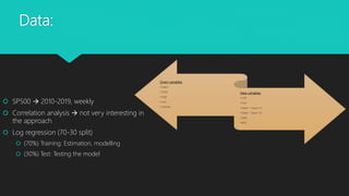
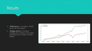
This document discusses using machine learning techniques to predict stock price movements. Specifically, it uses logistic regression on historical SP500 data to predict if the stock price will be higher or lower in the following week. Variables like open, close, volume and technical indicators are used as predictors. The model is trained on 70% of the data and tested on 30%. It achieves an accuracy of 65% on the test set, indicating the model performs well at predicting price movements. A backtest shows the strategy following the model's signals outperforms simply buying and holding the SP500. The summary concludes the approach is simple yet effective for this prediction problem.

1. Machine Learning : Stock
Price Prediction
Programming Techniques
Professor Carlos Costa
Master in Mathematical Finance
Diogo Bessa l53238
Iñigo Resco l53010
João Salgado l53231

2. Introduction
 Financial markets are essentially made by buying and selling
several types of financial instruments but it is also a complex and
dynamic system
 One of the hottest topics in financial markets is the stocks
 It is complicated to make the predictions of the stock price and
how it is going to move
 Few methods have been performed:
 Technical analysis (multiple regression types)
 Fundamental analysis

3. Objective
 The goal is to predict if the price of the stock in the following
week it is higher or lower according to the current week
 We used the Logistic Regression to give us the signal if the
price goes up (1) or goes down (-1)
 Our approach was based on choosing a sample, training our
model on it and testing the accuracy of it

4. Data:
Given variables
• Open
• Close
• High
• Low
• Volume
New variables
• m10
• Corr
• Open - Close (-1)
• Open - Open (-1)
• EMA
• ROC
 SP500  2010-2019, weekly
 Correlation analysis  not very interesting in
the approach
 Log regression (70-30 split)
 (70%) Training: Estimation, modelling
 (30%) Test: Testing the model

5. Model:
 Logistic regression
 Ability to make predictions on the dependent variable
 Train dataset
 Good estimator for a certain event occurring (M. Likelihood)
 Predicting class probs (P)  Dependent variable outcomes forced to
[-1 or 1]
 Model score and coefficients
𝑝 =
ex p( 𝛽0 + 𝑖=1
𝑝
𝛽𝑖 𝑋𝑖
1 + ex p( 𝛽0 + 𝑖=1
𝑝
𝛽𝑖 𝑋𝑖

6. Testing
 Predict p and force to [-1 or 1]
 Actual vs prediction  ACCURACY
Analysis of Classification report:
 Precision: number of true positives over
the number of true positives plus the
number of false positives.
 Recall: number of true positives over the
number of true positives plus the number
of false negatives.
 F1: weighted average of the precision and
recall F1 = 2 * (precision * recall) /
(precision + recall)

7. Testing
 K-Fold Cross validation test
 split your entire dataset into k”folds” (k=10)
 For 1st fold in your dataset, build your model on rest 9 folds of the
dataset. Then, test the model to check  take the error
 Repeat process and take average
 Almost same score as our model train set. Good approach
 0.63 vs 0.65

8. Results
Confusion matrix :
 Describes the performance of the model on the
test dataset for which the actual values are known
 (n=150)
 TP: 36
 TN: 62
 Acc= (36+62)/150 = 0.65

9. Results
 SP500 returns : Cumulative SP500
returns for test dataset.
 Strategy returns: Cumulative
strategy return based on the signal
predicted by the model in the test
dataset.

10. Conclusion
Our approach has a low
complexity and is easy to
understand or realize
The accuracy of the model
tell us the model’s
performance is good
Our strategy outperforms
the SP500 “long only”
traditional strategy
Can be used for further
future uses