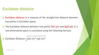
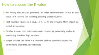
K-Nearest Neighbors
(KNN) --- Bayesian
Classification
Dr. Marwa M. Emam
Faculty of computers and Information
Minia University
Dr. Marwa M. Emam 1
Agenda
 Introduction to Nearest Neighbors (KNN)
 How KNN Works
 Mechanics of KNN
 Distance Metrics
 Explanation of Euclidean distance
 Choosing k
 Examples
 KNN-Classification
 KNN-Regression
 Naïve Bayes Algorithm
Dr. Marwa M. Emam 2
K-Nearest Neighbors (KNN)
 A KNN is a supervised learning algorithm used for both classification
and regression tasks.
 In case of classification, new data point get classified in a particular
class.
 In case of regression, new data point get labeled based on the AVR.
Value of KNN.
 Instance-Based: It's an instance-based learning algorithm, meaning it
makes predictions based on the closest instances in the training data.
 In instance-based learning, there is no explicit representation of a
model or a set of parameters that define the relationship between
input features and output.
3
K-Nearest Neighbors (KNN) …
 Instance-Based Learning:
 KNN belongs to the family of instance-based learning
algorithms.
 It doesn't build an explicit model during the training phase.
 Instead, it memorizes the entire training dataset.
 Closeness in Feature Space:
 Instances in the feature space are represented as points.
 The proximity or distance between points reflects their
similarity.
 The assumption is that instances with similar features should
have similar target values.
Dr. Marwa M. Emam 4
K-Nearest Neighbors (KNN) …
 Identifying Nearest Neighbors:
 During the prediction phase, KNN identifies the k-nearest
neighbors to a given data point.
 Neighbors are determined based on a distance metric,
commonly using Euclidean distance.
Dr. Marwa M. Emam 5
K-Nearest Neighbors (KNN) …
 Decision Making Through Classification or Regression:
 Classification:
 For classification tasks, KNN counts the occurrences of each class among
the k-neighbors.
 The majority class is assigned to the new data point.
 Regression:
 For regression tasks, KNN averages the target values of the k-neighbors.
 The average becomes the predicted value for the new data point.
Dr. Marwa M. Emam 6
K-Nearest Neighbors (KNN) …
 Choice of 'k':
 The parameter 'k' represents the number of neighbors
considered.
 The choice of 'k' is crucial and can impact the algorithm's
performance.
 Smaller 'k' values lead to more flexible models but may be
sensitive to noise.
 Larger 'k' values provide smoother decision boundaries but might
overlook local patterns.
Dr. Marwa M. Emam 7
Euclidean distance
 Euclidean distance is a measure of the straight-line distance between
two points in Euclidean space.
 The Euclidean distance between two points P(x1,y1) and Q(x2,y2) in a
two-dimensional space is calculated using the following formula:
 Euclidean Distance= (x2−x1)
2
+(y2−y1)
2
Dr. Marwa M. Emam 8
Euclidean distance …
 For a general case in n-dimensional space, where P and Q have coordinates
(x1,x2,...,xn) and (y1,y2,...,yn), the Euclidean distance is given by:
 𝑖=1
2
(𝑦𝑖 − 𝑋𝑖)2
 Straight-Line Distance: It represents the length of the shortest path (straight line)
between two points in space.
 Positive and Non-negative: Euclidean distance is always non-negative.
 Symmetric: The distance from point A to point B is the same as the distance from
point B to point A.
Dr. Marwa M. Emam 9
Example of a classification task using the K-
Nearest Neighbors (KNN) algorithm.
 Example Dataset: Iris Species Classification
 Consider a dataset of iris flowers with two features: sepal length and
sepal width. The goal is to classify iris flowers into two species:
Setosa and Versicolor.
Dr. Marwa M. Emam 10
Example …
Sepal Length Sepal Width Species
5.1 3.5 Setosa
4.9 3.0 Setosa
6.0 3.4 Versicolor
6.2 2.9 Versicolor
5.5 2.8 Versicolor
5.8 3.1 Setosa
6.7 3.1 Versicolor
5.6 3.0 Setosa
Dr. Marwa M. Emam 11
Suppose we have a new iris flower with Sepal Length = 5.5 and Sepal
Width = 3.2. Predict it Species????
Solution
 Calculate Euclidean Distances:
 Calculate the Euclidean distance between the new point and all points in
the training set.
 Select 'k' Nearest Neighbors:
 Choose a value for 'k' (number of neighbors), e.g., k = 3.
 Identify the three training points with the shortest distances to the new
point.
 Majority Voting:
 Determine the majority class among the selected neighbors.
 If, for example, two neighbors are Setosa and one is Versicolor, the prediction is
Setosa.
Dr. Marwa M. Emam
12
Solution …
 KNN Classification Process:
 Calculate Euclidean Distances:
 Calculate the Euclidean distance between the new point (5.5, 3.2) and all
points in the training set.
Dr. Marwa M. Emam 13
Euclidean Distance= (x2−x1)
𝟐
+(y2−y1)
𝟐
Dr. Marwa M. Emam
14
Training Point Euclidean Distance
Setosa (5.1, 3.5) (5.1−5.5)
𝟐
+(3.5−3.2)
𝟐
=0.848
Setosa (4.9, 3.0) (4.9−5.5)𝟐
+(3.0−3.2)𝟐
=0.282
Versicolor (6.0, 3.4) (6.0−5.5)
𝟐
+(3.4−3.2)
𝟐
=1.104
Versicolor (6.2, 2.9) (6.2−5.5)
𝟐
+(2.9−3.2)
𝟐
=1.521
Versicolor (5.5, 2.8) (5.5−5.5)
𝟐
+(3.1−3.2)
𝟐
=0.447
Setosa (5.8, 3.1) (5.8−5.5)
𝟐
+(3.1−3.2)
𝟐
=0.412
Versicolor (6.7, 3.1) (6.7−5.5)
𝟐
+(3.1−3.2)
𝟐
=1.275
Setosa (5.6, 3.0) (5.6−5.5)
𝟐
+(3.0−3.2)𝟐
=0.360
Solution …
 Select 'k' Nearest Neighbors:
 Choose k = 3.
 The three nearest neighbors are those with the smallest Euclidean
distances: Setosa (4.9, 3.0), Setosa (5.6, 3.0), Setosa (5.8, 3.1)
 Majority Voting:
 The majority class among the selected neighbors is Setosa.
 Prediction: The new iris flower is predicted to be Setosa.
Dr. Marwa M. Emam 15
Solution ….
 Select 'k' Nearest Neighbors:
 Choose k = 3.
 The three nearest neighbors are the ones with the smallest
Euclidean distances.
 Nearest Neighbors: Setosa (4.9, 3.0), Setosa (5.6, 3.0),
Setosa (5.8, 3.1)
 Majority Voting:
 The majority class among the selected neighbors is Setosa.
 Prediction: The new iris flower is predicted to be Setosa.
Dr. Marwa M. Emam 16
How to choose the K value
 For binary classification problems, it's often recommended to use an odd
value for k to avoid ties in voting, ensuring a clear majority.
 Test multiple values for k (e.g., 3, 5, 7, 9) and evaluate their impact on
model performance.
 Smaller k values tend to increase model complexity, potentially leading to
overfitting (low bias, high variance).
 Larger k values can result in a smoother decision boundary, potentially
underfitting (high bias, low variance).
Dr. Marwa M. Emam 17
KNN Regression
 Example Dataset: House Price Regression
 Regression Task: Predicting House Prices
 Suppose we want to predict the price of a house with 1800 square footage
and 3 bedrooms.
Dr. Marwa M. Emam
18
Square Footage Bedrooms House Price
1500 3 250.000
2000 4 320.000
1200 2 180.000
1800 3 270.000
2500 4 400.000
1400 2 200.000
KNN Regression …
Solution
 Calculate Euclidean Distances:
 Calculate the Euclidean distance between the new point (1800 sq. ft.,
3 bedrooms) and all points in the training set:
 Distance= (Sq. Ft.2−Sq. Ft.1)2+(Bedrooms2−Bedrooms1)2
Dr. Marwa M. Emam 19
Training
Point Sq. Ft. Bedrooms House Price
Euclidean
Distance
1 1500 3 250,000 300
2 2000 4 320,000 200
3 1200 2 180,000 600
4 1800 3 270,000 0
5 2500 4 400,000 700
6 1400 2 200,000 400
Dr. Marwa M. Emam
20
Select 'k' Nearest Neighbors:
•Choose k=3.
•Identify the three training points with the smallest Euclidean distances:
•Nearest Neighbors:
• Point 2 (2000 sq. ft., 4 bedrooms) - House Price: $320,000
• Point 6 (1400 sq. ft., 2 bedrooms) - House Price: $200,000
• Point 4 (1800 sq. ft., 3 bedrooms) - House Price: $270,000
KNN Regression …
Solution
 Regression:
 For regression, we take the average of the target values (house
prices) of the k nearest neighbors:
 Predicted Price=320,000+200,000+270,000/3
 Predicted Price=790,000/3
 Predicted Price≈263,333.33
Dr. Marwa M. Emam 21
Bayesian Classification
Dr. Marwa M. Emam 22
Overview
 The Bayesian classifier is an algorithm for classifying multi-class
datasets.
 This is based on the Bayes’ theorem in probability theory with an
assumption of independence among predictors.
 The classifier is also known as “naive Bayes Algorithm” where
the word “naive” is an English word with the following meanings:
simple, unsophisticated, or primitive.
Dr. Marwa M. Emam 23
Naive Bayes (NB) Algorithm
 Naive Bayes is a probabilistic machine learning algorithm that is based on
Bayes' theorem.
 It is primarily used for classification tasks but can also be extended to
handle regression.
 The "naive" assumption made by the algorithm is that the features used to
describe instances are conditionally independent, given the class label.
 This assumption simplifies the calculation of probabilities and makes the
algorithm computationally efficient.
Dr. Marwa M. Emam 24
Bayes' Theorem
 Bayes' theorem provides a way to update the probability of a hypothesis based on
evidence:
 P(A∣B)=
P(B∣A)⋅P(A)
P(B)
 P(A∣B): Probability of hypothesis A given evidence B.
 P(B∣A): Probability of evidence B given hypothesis A.
 P(A): Prior probability of hypothesis A.
 P(B): Prior probability of evidence B.
Dr. Marwa M. Emam 25
Naive Bayes Algorithm
 Input:
 X (Input Features):
 Represents the features used to describe instances. For example, in a document classification
task, these features could be words present in the document.
 C (Class Labels):
 Denotes the class labels associated with the instances. In document classification, classes
might be categories like "spam" or "not spam.”
 Training:
 Step 1: Calculate Prior Probabilities P(C):
 Objective:
 Determine the prior probability of each class, representing the likelihood of a class occurring
without considering any features.
 Calculation:
 P(C) is calculated based on the frequency or proportion of instances in each class in the
training dataset.
Dr. Marwa M. Emam
26
Naive Bayes Algorithm ..
 Step 2: Calculate the likelihood P(X∣C) for each feature given
the class.
 Objective:
 Estimate the likelihood of observing the given features X given a specific class C.
 Calculation:
 For each feature xi in X, calculate P(xi∣C) using the training data.
 Step 3: Apply the naive assumption that features are
conditionally independent: P(X∣C)=P(x1∣C)⋅P(x2∣C)⋅…⋅P(xn∣C).
 Step 4: Calculate Posterior Probabilities P(C∣X):
Dr. Marwa M. Emam 27
Naive Bayes Algorithm ..
 Use Bayes' theorem: P(C∣X)=
P(X∣C)⋅P(C)
P(X)
.
 The denominator P(X) acts as a normalization factor.
 Prediction:
 Given a new instance with features Xnew, calculate
P(C∣Xnew) for each class.
 Assign the class with the highest posterior probability as
the predicted class.
Dr. Marwa M. Emam 28
Example: Spam Email Classification using
Naive Bayes
29
 A simple example of classifying emails as either spam or not spam
using the Naive Bayes algorithm. For simplicity, we'll focus on just two
features: the presence of the word "lottery" and the presence of the
word " Discount.“
Email Discount Lottery Class
Get a discount today! Yes No spam
Win a lottery ticket No Yes Spam
Exclusive offer
Yes
No spam
Meeting tomorrow NO NO Not Spam
Lottery winner No yes spam
Example: Spam Email Classification using
Naive Bayes …
 Step 1: Calculate Prior Probabilities P(Class):
 Calculate P(Spam) and P(Not Spam).
 P(Spam)=Number of Spam Emails / Total Emails.
 P(Not Spam)=Number of Not Spam Emails / Total Emails.
 Step 2: Calculate P(word∣Class):
 Calculate P(Discount∣Spam), P(Lottery∣Spam), P(Discount∣Not Spam),
P(Lottery∣Not Spam).
 Step 3: Apply the Naive Assumption:
 Assume that the occurrence of words is independent given the class.
 P(Discount,Lottery∣Spam)=P(Discount∣Spam)⋅P(Lottery∣Spam)
 P(Discount,Lottery∣NotSpam)=P(Discount∣Spam)⋅P(Lottery∣Spam)
Dr. Marwa M. Emam
30
Example: Spam Email Classification using
Naive Bayes …
 Step 4: Calculate Posterior Probabilities P(Class∣Email):
 Use Bayes' theorem to calculate P(Spam∣Email) and
P(Not Spam∣Email).
Dr. Marwa M. Emam 31
The Example solution
 Step 1: Calculate Prior Probabilities P(Class):
 Calculate P(Spam) and P(Not Spam):
 P(Spam)= 4/5
 P(Not Spam)= 1/5
 Step 2: Calculate P(Word∣Class):

Dr. Marwa M. Emam
32
The Example solution …
 Step 3: Apply the Naive Assumption:
Dr. Marwa M. Emam
33
Task
Dr. Marwa M. Emam 34
Thanks
Dr. Marwa M. Emam 35

Machine Learning-Lec7 Bayesian calssification.pdf

  • 1.
    K-Nearest Neighbors (KNN) ---Bayesian Classification Dr. Marwa M. Emam Faculty of computers and Information Minia University Dr. Marwa M. Emam 1
  • 2.
    Agenda  Introduction toNearest Neighbors (KNN)  How KNN Works  Mechanics of KNN  Distance Metrics  Explanation of Euclidean distance  Choosing k  Examples  KNN-Classification  KNN-Regression  Naïve Bayes Algorithm Dr. Marwa M. Emam 2
  • 3.
    K-Nearest Neighbors (KNN) A KNN is a supervised learning algorithm used for both classification and regression tasks.  In case of classification, new data point get classified in a particular class.  In case of regression, new data point get labeled based on the AVR. Value of KNN.  Instance-Based: It's an instance-based learning algorithm, meaning it makes predictions based on the closest instances in the training data.  In instance-based learning, there is no explicit representation of a model or a set of parameters that define the relationship between input features and output. 3
  • 4.
    K-Nearest Neighbors (KNN)…  Instance-Based Learning:  KNN belongs to the family of instance-based learning algorithms.  It doesn't build an explicit model during the training phase.  Instead, it memorizes the entire training dataset.  Closeness in Feature Space:  Instances in the feature space are represented as points.  The proximity or distance between points reflects their similarity.  The assumption is that instances with similar features should have similar target values. Dr. Marwa M. Emam 4
  • 5.
    K-Nearest Neighbors (KNN)…  Identifying Nearest Neighbors:  During the prediction phase, KNN identifies the k-nearest neighbors to a given data point.  Neighbors are determined based on a distance metric, commonly using Euclidean distance. Dr. Marwa M. Emam 5
  • 6.
    K-Nearest Neighbors (KNN)…  Decision Making Through Classification or Regression:  Classification:  For classification tasks, KNN counts the occurrences of each class among the k-neighbors.  The majority class is assigned to the new data point.  Regression:  For regression tasks, KNN averages the target values of the k-neighbors.  The average becomes the predicted value for the new data point. Dr. Marwa M. Emam 6
  • 7.
    K-Nearest Neighbors (KNN)…  Choice of 'k':  The parameter 'k' represents the number of neighbors considered.  The choice of 'k' is crucial and can impact the algorithm's performance.  Smaller 'k' values lead to more flexible models but may be sensitive to noise.  Larger 'k' values provide smoother decision boundaries but might overlook local patterns. Dr. Marwa M. Emam 7
  • 8.
    Euclidean distance  Euclideandistance is a measure of the straight-line distance between two points in Euclidean space.  The Euclidean distance between two points P(x1,y1) and Q(x2,y2) in a two-dimensional space is calculated using the following formula:  Euclidean Distance= (x2−x1) 2 +(y2−y1) 2 Dr. Marwa M. Emam 8
  • 9.
    Euclidean distance … For a general case in n-dimensional space, where P and Q have coordinates (x1,x2,...,xn) and (y1,y2,...,yn), the Euclidean distance is given by:  𝑖=1 2 (𝑦𝑖 − 𝑋𝑖)2  Straight-Line Distance: It represents the length of the shortest path (straight line) between two points in space.  Positive and Non-negative: Euclidean distance is always non-negative.  Symmetric: The distance from point A to point B is the same as the distance from point B to point A. Dr. Marwa M. Emam 9
  • 10.
    Example of aclassification task using the K- Nearest Neighbors (KNN) algorithm.  Example Dataset: Iris Species Classification  Consider a dataset of iris flowers with two features: sepal length and sepal width. The goal is to classify iris flowers into two species: Setosa and Versicolor. Dr. Marwa M. Emam 10
  • 11.
    Example … Sepal LengthSepal Width Species 5.1 3.5 Setosa 4.9 3.0 Setosa 6.0 3.4 Versicolor 6.2 2.9 Versicolor 5.5 2.8 Versicolor 5.8 3.1 Setosa 6.7 3.1 Versicolor 5.6 3.0 Setosa Dr. Marwa M. Emam 11 Suppose we have a new iris flower with Sepal Length = 5.5 and Sepal Width = 3.2. Predict it Species????
  • 12.
    Solution  Calculate EuclideanDistances:  Calculate the Euclidean distance between the new point and all points in the training set.  Select 'k' Nearest Neighbors:  Choose a value for 'k' (number of neighbors), e.g., k = 3.  Identify the three training points with the shortest distances to the new point.  Majority Voting:  Determine the majority class among the selected neighbors.  If, for example, two neighbors are Setosa and one is Versicolor, the prediction is Setosa. Dr. Marwa M. Emam 12
  • 13.
    Solution …  KNNClassification Process:  Calculate Euclidean Distances:  Calculate the Euclidean distance between the new point (5.5, 3.2) and all points in the training set. Dr. Marwa M. Emam 13 Euclidean Distance= (x2−x1) 𝟐 +(y2−y1) 𝟐
  • 14.
    Dr. Marwa M.Emam 14 Training Point Euclidean Distance Setosa (5.1, 3.5) (5.1−5.5) 𝟐 +(3.5−3.2) 𝟐 =0.848 Setosa (4.9, 3.0) (4.9−5.5)𝟐 +(3.0−3.2)𝟐 =0.282 Versicolor (6.0, 3.4) (6.0−5.5) 𝟐 +(3.4−3.2) 𝟐 =1.104 Versicolor (6.2, 2.9) (6.2−5.5) 𝟐 +(2.9−3.2) 𝟐 =1.521 Versicolor (5.5, 2.8) (5.5−5.5) 𝟐 +(3.1−3.2) 𝟐 =0.447 Setosa (5.8, 3.1) (5.8−5.5) 𝟐 +(3.1−3.2) 𝟐 =0.412 Versicolor (6.7, 3.1) (6.7−5.5) 𝟐 +(3.1−3.2) 𝟐 =1.275 Setosa (5.6, 3.0) (5.6−5.5) 𝟐 +(3.0−3.2)𝟐 =0.360
  • 15.
    Solution …  Select'k' Nearest Neighbors:  Choose k = 3.  The three nearest neighbors are those with the smallest Euclidean distances: Setosa (4.9, 3.0), Setosa (5.6, 3.0), Setosa (5.8, 3.1)  Majority Voting:  The majority class among the selected neighbors is Setosa.  Prediction: The new iris flower is predicted to be Setosa. Dr. Marwa M. Emam 15
  • 16.
    Solution ….  Select'k' Nearest Neighbors:  Choose k = 3.  The three nearest neighbors are the ones with the smallest Euclidean distances.  Nearest Neighbors: Setosa (4.9, 3.0), Setosa (5.6, 3.0), Setosa (5.8, 3.1)  Majority Voting:  The majority class among the selected neighbors is Setosa.  Prediction: The new iris flower is predicted to be Setosa. Dr. Marwa M. Emam 16
  • 17.
    How to choosethe K value  For binary classification problems, it's often recommended to use an odd value for k to avoid ties in voting, ensuring a clear majority.  Test multiple values for k (e.g., 3, 5, 7, 9) and evaluate their impact on model performance.  Smaller k values tend to increase model complexity, potentially leading to overfitting (low bias, high variance).  Larger k values can result in a smoother decision boundary, potentially underfitting (high bias, low variance). Dr. Marwa M. Emam 17
  • 18.
    KNN Regression  ExampleDataset: House Price Regression  Regression Task: Predicting House Prices  Suppose we want to predict the price of a house with 1800 square footage and 3 bedrooms. Dr. Marwa M. Emam 18 Square Footage Bedrooms House Price 1500 3 250.000 2000 4 320.000 1200 2 180.000 1800 3 270.000 2500 4 400.000 1400 2 200.000
  • 19.
    KNN Regression … Solution Calculate Euclidean Distances:  Calculate the Euclidean distance between the new point (1800 sq. ft., 3 bedrooms) and all points in the training set:  Distance= (Sq. Ft.2−Sq. Ft.1)2+(Bedrooms2−Bedrooms1)2 Dr. Marwa M. Emam 19
  • 20.
    Training Point Sq. Ft.Bedrooms House Price Euclidean Distance 1 1500 3 250,000 300 2 2000 4 320,000 200 3 1200 2 180,000 600 4 1800 3 270,000 0 5 2500 4 400,000 700 6 1400 2 200,000 400 Dr. Marwa M. Emam 20 Select 'k' Nearest Neighbors: •Choose k=3. •Identify the three training points with the smallest Euclidean distances: •Nearest Neighbors: • Point 2 (2000 sq. ft., 4 bedrooms) - House Price: $320,000 • Point 6 (1400 sq. ft., 2 bedrooms) - House Price: $200,000 • Point 4 (1800 sq. ft., 3 bedrooms) - House Price: $270,000
  • 21.
    KNN Regression … Solution Regression:  For regression, we take the average of the target values (house prices) of the k nearest neighbors:  Predicted Price=320,000+200,000+270,000/3  Predicted Price=790,000/3  Predicted Price≈263,333.33 Dr. Marwa M. Emam 21
  • 22.
  • 23.
    Overview  The Bayesianclassifier is an algorithm for classifying multi-class datasets.  This is based on the Bayes’ theorem in probability theory with an assumption of independence among predictors.  The classifier is also known as “naive Bayes Algorithm” where the word “naive” is an English word with the following meanings: simple, unsophisticated, or primitive. Dr. Marwa M. Emam 23
  • 24.
    Naive Bayes (NB)Algorithm  Naive Bayes is a probabilistic machine learning algorithm that is based on Bayes' theorem.  It is primarily used for classification tasks but can also be extended to handle regression.  The "naive" assumption made by the algorithm is that the features used to describe instances are conditionally independent, given the class label.  This assumption simplifies the calculation of probabilities and makes the algorithm computationally efficient. Dr. Marwa M. Emam 24
  • 25.
    Bayes' Theorem  Bayes'theorem provides a way to update the probability of a hypothesis based on evidence:  P(A∣B)= P(B∣A)⋅P(A) P(B)  P(A∣B): Probability of hypothesis A given evidence B.  P(B∣A): Probability of evidence B given hypothesis A.  P(A): Prior probability of hypothesis A.  P(B): Prior probability of evidence B. Dr. Marwa M. Emam 25
  • 26.
    Naive Bayes Algorithm Input:  X (Input Features):  Represents the features used to describe instances. For example, in a document classification task, these features could be words present in the document.  C (Class Labels):  Denotes the class labels associated with the instances. In document classification, classes might be categories like "spam" or "not spam.”  Training:  Step 1: Calculate Prior Probabilities P(C):  Objective:  Determine the prior probability of each class, representing the likelihood of a class occurring without considering any features.  Calculation:  P(C) is calculated based on the frequency or proportion of instances in each class in the training dataset. Dr. Marwa M. Emam 26
  • 27.
    Naive Bayes Algorithm..  Step 2: Calculate the likelihood P(X∣C) for each feature given the class.  Objective:  Estimate the likelihood of observing the given features X given a specific class C.  Calculation:  For each feature xi in X, calculate P(xi∣C) using the training data.  Step 3: Apply the naive assumption that features are conditionally independent: P(X∣C)=P(x1∣C)⋅P(x2∣C)⋅…⋅P(xn∣C).  Step 4: Calculate Posterior Probabilities P(C∣X): Dr. Marwa M. Emam 27
  • 28.
    Naive Bayes Algorithm..  Use Bayes' theorem: P(C∣X)= P(X∣C)⋅P(C) P(X) .  The denominator P(X) acts as a normalization factor.  Prediction:  Given a new instance with features Xnew, calculate P(C∣Xnew) for each class.  Assign the class with the highest posterior probability as the predicted class. Dr. Marwa M. Emam 28
  • 29.
    Example: Spam EmailClassification using Naive Bayes 29  A simple example of classifying emails as either spam or not spam using the Naive Bayes algorithm. For simplicity, we'll focus on just two features: the presence of the word "lottery" and the presence of the word " Discount.“ Email Discount Lottery Class Get a discount today! Yes No spam Win a lottery ticket No Yes Spam Exclusive offer Yes No spam Meeting tomorrow NO NO Not Spam Lottery winner No yes spam
  • 30.
    Example: Spam EmailClassification using Naive Bayes …  Step 1: Calculate Prior Probabilities P(Class):  Calculate P(Spam) and P(Not Spam).  P(Spam)=Number of Spam Emails / Total Emails.  P(Not Spam)=Number of Not Spam Emails / Total Emails.  Step 2: Calculate P(word∣Class):  Calculate P(Discount∣Spam), P(Lottery∣Spam), P(Discount∣Not Spam), P(Lottery∣Not Spam).  Step 3: Apply the Naive Assumption:  Assume that the occurrence of words is independent given the class.  P(Discount,Lottery∣Spam)=P(Discount∣Spam)⋅P(Lottery∣Spam)  P(Discount,Lottery∣NotSpam)=P(Discount∣Spam)⋅P(Lottery∣Spam) Dr. Marwa M. Emam 30
  • 31.
    Example: Spam EmailClassification using Naive Bayes …  Step 4: Calculate Posterior Probabilities P(Class∣Email):  Use Bayes' theorem to calculate P(Spam∣Email) and P(Not Spam∣Email). Dr. Marwa M. Emam 31
  • 32.
    The Example solution Step 1: Calculate Prior Probabilities P(Class):  Calculate P(Spam) and P(Not Spam):  P(Spam)= 4/5  P(Not Spam)= 1/5  Step 2: Calculate P(Word∣Class):  Dr. Marwa M. Emam 32
  • 33.
    The Example solution…  Step 3: Apply the Naive Assumption: Dr. Marwa M. Emam 33
  • 34.
  • 35.