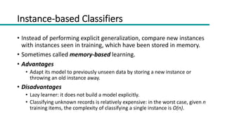
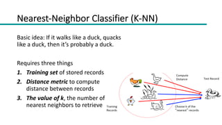
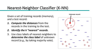
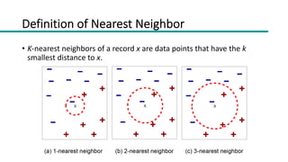
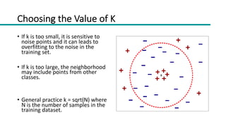
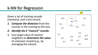
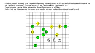
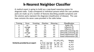
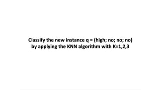
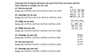
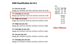
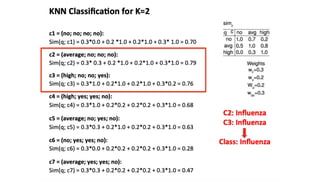
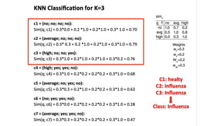
DATA MINING 1
Instance-based Classifiers
Dino Pedreschi, Riccardo Guidotti
a.a. 2022/2023
Slides edited from Tan, Steinbach, Kumar, Introduction to Data Mining
Instance-based Classifiers
• Instead of performing explicit generalization, compare new instances
with instances seen in training, which have been stored in memory.
• Sometimes called memory-based learning.
• Advantages
• Adapt its model to previously unseen data by storing a new instance or
throwing an old instance away.
• Disadvantages
• Lazy learner: it does not build a model explicitly.
• Classifying unknown records is relatively expensive: in the worst case, given n
training items, the complexity of classifying a single instance is O(n).
Nearest-Neighbor Classifier (K-NN)
Basic idea: If it walks like a duck, quacks
like a duck, then it’s probably a duck.
Requires three things
1. Training set of stored records
2. Distance metric to compute
distance between records
3. The value of k, the number of
nearest neighbors to retrieve
Nearest-Neighbor Classifier (K-NN)
Given a set of training records (memory),
and a test record:
1. Compute the distances from the
records in the training to the test.
2. Identify the k “nearest” records.
3. Use class labels of nearest neighbors to
determine the class label of unknown
record (e.g., by taking majority vote).
Definition of Nearest Neighbor
• K-nearest neighbors of a record x are data points that have the k
smallest distance to x.
Choosing the Value of K
• If k is too small, it is sensitive to
noise points and it can leads to
overfitting to the noise in the
training set.
• If k is too large, the neighborhood
may include points from other
classes.
• General practice k = sqrt(N) where
N is the number of samples in the
training dataset.
Nearest Neighbor Classification
Compute distance between two points:
• Euclidean distance 𝑑 𝑝, 𝑞 = ∑!(𝑝! − 𝑞!)"
Determine the class from nearest neighbors
• take the majority vote of class labels among the k nearest neighbors
• weigh the vote according to distance (e.g. weight factor, w = 1/d2)
Dimensionality and Scaling Issues
• Problem with Euclidean measure: high dimensional data can cause
curse of dimensionality.
• Solution: normalize the vectors to unit length
• Attributes may have to be scaled to prevent distance measures from
being dominated by one of the attributes.
• Example:
• height of a person may vary from 1.5m to 1.8m
• weight of a person may vary from 10km to 200kg
• income of a person may vary from $10K to $1M
Parallel Exemplar-Based Learning System (PEBLS)
• PEBLS is a nearest-neighbor learning system (k=1) designed for
applications where the instances have symbolic feature values.
• Works with both continuous and nominal features.
• For nominal features, the distance between two nominal values is
computed using Modified Value Difference Metric (MVDM)
• 𝑑 𝑉#, 𝑉" = ∑! |
$!"
$!
−
$#"
$#
|
• Where n1 is the number of records that consists of nominal attribute
value V1 and n1i is the number of records whose target label is class i.
Distance Between Nominal Attribute Values
• d(Status=Single, Status=Married) = | 2/4 – 0/4 | + | 2/4 – 4/4 | = 1
• d(Status=Single, Status=Divorced) = | 2/4 – 1/2 | + | 2/4 – 1/2 | = 0
• d(Status=Married, Status=Divorced) = | 0/4 – 1/2 | + | 4/4 – 1/2 | = 1
• d(Refund=Yes, Refund=No) = | 0/3 – 3/7 | + | 3/3 – 4/7 | = 6/7
Distance Between Records
• 𝛿 𝑋, 𝑌 = 𝑤!𝑤" ∑#$%
&
𝑑(𝑋#, 𝑌#)
• Each record X is assigned a weight 𝑤! =
'!"#$%&'(
'!"#$%&'(
')##$'(
, which represents its reliability
• 𝑁!"#$%&'(
is the number of times X is used for prediction
• 𝑁!"#$%&'(
')##$'( is the number of times the prediction using X is correct
• If 𝑤! ≅ 1 X makes accurate prediction most of the time
• If 𝑤!> 1, then X is not reliable for making predictions. High 𝑤! >1 would result in
high distance, which makes it less possible to use X to make predictions.
Characteristics of Nearest Neighbor Classifiers
• Instance-based learner: makes predictions without maintaining
abstraction, i.e., building a model like decision trees.
• It is a lazy learner: classifying a test example can be expensive because
need to compute the proximity values between test and training examples.
• In contrast eager learners spend time in building the model but then the
classification is fast.
• Make their prediction on local information and for low k they are
susceptible to noise.
• Can produce wrong predictions if inappropriate distance functions and/or
preprocessing steps are performed.
k-NN for Regression
Given a set of training records
(memory), and a test record:
1. Compute the distances from the
records in the training to the test.
2. Identify the k “nearest” records.
3. Use target value of nearest
neighbors to determine the value
of unknown record (e.g., by
averaging the values).
3.4
5.4
5.7
8.7
9.7
3.9
3.8
4.1
5.1
4.3
10.3 9.2
3.2
5.9
4.7
12.1
10.8
8.7
9.7
3.4
4.2
References
• Nearest Neighbor classifiers. Chapter 5.2.
Introduction to Data Mining.
Exercises - kNN
09_dm1_knn_2022_23.pdf

09_dm1_knn_2022_23.pdf

  • 1.
    DATA MINING 1 Instance-basedClassifiers Dino Pedreschi, Riccardo Guidotti a.a. 2022/2023 Slides edited from Tan, Steinbach, Kumar, Introduction to Data Mining
  • 2.
    Instance-based Classifiers • Insteadof performing explicit generalization, compare new instances with instances seen in training, which have been stored in memory. • Sometimes called memory-based learning. • Advantages • Adapt its model to previously unseen data by storing a new instance or throwing an old instance away. • Disadvantages • Lazy learner: it does not build a model explicitly. • Classifying unknown records is relatively expensive: in the worst case, given n training items, the complexity of classifying a single instance is O(n).
  • 3.
    Nearest-Neighbor Classifier (K-NN) Basicidea: If it walks like a duck, quacks like a duck, then it’s probably a duck. Requires three things 1. Training set of stored records 2. Distance metric to compute distance between records 3. The value of k, the number of nearest neighbors to retrieve
  • 4.
    Nearest-Neighbor Classifier (K-NN) Givena set of training records (memory), and a test record: 1. Compute the distances from the records in the training to the test. 2. Identify the k “nearest” records. 3. Use class labels of nearest neighbors to determine the class label of unknown record (e.g., by taking majority vote).
  • 5.
    Definition of NearestNeighbor • K-nearest neighbors of a record x are data points that have the k smallest distance to x.
  • 6.
    Choosing the Valueof K • If k is too small, it is sensitive to noise points and it can leads to overfitting to the noise in the training set. • If k is too large, the neighborhood may include points from other classes. • General practice k = sqrt(N) where N is the number of samples in the training dataset.
  • 7.
    Nearest Neighbor Classification Computedistance between two points: • Euclidean distance 𝑑 𝑝, 𝑞 = ∑!(𝑝! − 𝑞!)" Determine the class from nearest neighbors • take the majority vote of class labels among the k nearest neighbors • weigh the vote according to distance (e.g. weight factor, w = 1/d2)
  • 8.
    Dimensionality and ScalingIssues • Problem with Euclidean measure: high dimensional data can cause curse of dimensionality. • Solution: normalize the vectors to unit length • Attributes may have to be scaled to prevent distance measures from being dominated by one of the attributes. • Example: • height of a person may vary from 1.5m to 1.8m • weight of a person may vary from 10km to 200kg • income of a person may vary from $10K to $1M
  • 9.
    Parallel Exemplar-Based LearningSystem (PEBLS) • PEBLS is a nearest-neighbor learning system (k=1) designed for applications where the instances have symbolic feature values. • Works with both continuous and nominal features. • For nominal features, the distance between two nominal values is computed using Modified Value Difference Metric (MVDM) • 𝑑 𝑉#, 𝑉" = ∑! | $!" $! − $#" $# | • Where n1 is the number of records that consists of nominal attribute value V1 and n1i is the number of records whose target label is class i.
  • 10.
    Distance Between NominalAttribute Values • d(Status=Single, Status=Married) = | 2/4 – 0/4 | + | 2/4 – 4/4 | = 1 • d(Status=Single, Status=Divorced) = | 2/4 – 1/2 | + | 2/4 – 1/2 | = 0 • d(Status=Married, Status=Divorced) = | 0/4 – 1/2 | + | 4/4 – 1/2 | = 1 • d(Refund=Yes, Refund=No) = | 0/3 – 3/7 | + | 3/3 – 4/7 | = 6/7
  • 11.
    Distance Between Records •𝛿 𝑋, 𝑌 = 𝑤!𝑤" ∑#$% & 𝑑(𝑋#, 𝑌#) • Each record X is assigned a weight 𝑤! = '!"#$%&'( '!"#$%&'( ')##$'( , which represents its reliability • 𝑁!"#$%&'( is the number of times X is used for prediction • 𝑁!"#$%&'( ')##$'( is the number of times the prediction using X is correct • If 𝑤! ≅ 1 X makes accurate prediction most of the time • If 𝑤!> 1, then X is not reliable for making predictions. High 𝑤! >1 would result in high distance, which makes it less possible to use X to make predictions.
  • 12.
    Characteristics of NearestNeighbor Classifiers • Instance-based learner: makes predictions without maintaining abstraction, i.e., building a model like decision trees. • It is a lazy learner: classifying a test example can be expensive because need to compute the proximity values between test and training examples. • In contrast eager learners spend time in building the model but then the classification is fast. • Make their prediction on local information and for low k they are susceptible to noise. • Can produce wrong predictions if inappropriate distance functions and/or preprocessing steps are performed.
  • 13.
    k-NN for Regression Givena set of training records (memory), and a test record: 1. Compute the distances from the records in the training to the test. 2. Identify the k “nearest” records. 3. Use target value of nearest neighbors to determine the value of unknown record (e.g., by averaging the values). 3.4 5.4 5.7 8.7 9.7 3.9 3.8 4.1 5.1 4.3 10.3 9.2 3.2 5.9 4.7 12.1 10.8 8.7 9.7 3.4 4.2
  • 14.
    References • Nearest Neighborclassifiers. Chapter 5.2. Introduction to Data Mining.
  • 15.