Machine learning Experiments report

Machine Learning Lab Report
Submitted by:
Almkdad Ali, MCS18001
Course:
M. Tech, CSE
Date:
16-April-2019
C. V. Raman College of Engineering, Department of Computer Science and Engineering

1
Table of Contents
1. Tools and Libraries…………………………………………………….....……………. 2
2. Experiment 1 (ANN, Backpropagation)................................................................... 8
3. Experiment 2 (K-Means Algorithm)......................................................................... 13
4. Experiment 3 (Hierarchical Clustering)................................................................... 18
5. Experiment 4 (Linear regression,Multivariate Regression)................................... 24
6. Experiment 5 (Fuzzy Logic)....................................................................................... 31
7. Assignment ( Fuzzy Logic, Defuzzification Methods) …………………………..… 38

2
1.Tools and Libraries:
1.1 Python:
1.1.1 What is Python?
● Python is an interpreted programming language used in various
fields.
● It has two major versions 2.X, and 3.X.
● It used in :
○ web development (server-side),
○ software development,
○ mathematics,
○ system scripting.
○ Scientific applications.
1.1.2 What can Python do?
● Python can be used on a server to create web applications.
● Python can be used alongside software to create workflows.
● Python can connect to database systems. It can also read and
modify files.
● Python can be used to handle big data and perform complex
mathematics.
● Python can be used for rapid prototyping, or for production-ready
software development.
1.1.3 Why using Python?
● Python works on different platforms (Windows, Mac, Linux, Raspberry Pi,
etc).
● Python has a simple syntax similar to the English language.
● Python has syntax that allows developers to write programs with fewer
lines than some other programming languages.
● Python runs on an interpreter system, meaning that code can be
executed as soon as it is written. This means that prototyping can be very
quick.
● Python can be treated in a procedural way, an object-oriented way or a
functional way.

3
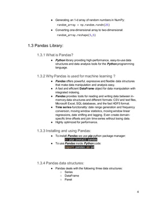
1.2 NumPy Library:
1.2.1 What is NumPy?
● NumPy is the fundamental package for scientific computing with
Python.
● It contains among other things:
○ a powerful N-dimensional array object
○ sophisticated (broadcasting) functions
○ tools for integrating C/C++ and Fortran code
○ useful linear algebra, Fourier transform, and random
number capabilities
1.2.2 Why NumPy is useful for machine learning?
● NumPy is very useful for performing mathematical and logical
operations on Arrays.
● It provides an abundance of useful features for operations on n-
arrays and matrices in Python.
1.2.3 Installing and using NumPy
● To install NumPy we use pip python package manager:
>> pip install numpy
● To use NumPy inside Python code:
import numpy as np
1.2.4 NumPy arrays:
● A NumPy array is simply a grid that contains values of the same
type.
● NumPy Arrays come in two forms; Vectors and Matrices.
● Vectors are strictly one-dimensional(1-d) arrays.
● Matrices are multidimensional.
● In some cases, Matrices can still have only one row or one
column.
● Using NumPy array in code:
python_list = [[1,2,3], [5,4,1], [3,6,7]]
new_2d_arr = np.array(second_list)
● Creating array from range:
my_list = np.arange(0,10)
● Generate a one-dimensional array of zeros:
zeros_array = np.zeros(5)

4
● Generating an 1-d array of random numbers in NumPy:
random_array = np.random.randn(25)
● Converting one-dimensional array to two-dimensional:
random_array.reshape(5,5)
1.3 Pandas Library:
1.3.1 What is Pandas?
● Python library providing high-performance, easy-to-use data
structures and data analysis tools for the Python programming
language.
1.3.2 Why Pandas is used for machine learning ?
● Pandas offers powerful, expressive and flexible data structures
that make data manipulation and analysis easy.
● A fast and efficient DataFrame object for data manipulation with
integrated indexing.
● Pandas provides tools for reading and writing data between in-
memory data structures and different formats: CSV and text files,
Microsoft Excel, SQL databases, and the fast HDF5 format.
● Time series-functionality: date range generation and frequency
conversion, moving window statistics, moving window linear
regressions, date shifting and lagging. Even create domain-
specific time offsets and join time series without losing data.
● Highly optimized for performance.
1.3.3 Installing and using Pandas:
● To install Pandas we use pip python package manager:
>> pip install pandas
● To use Pandas inside Python code:
import pandas as pd
1.3.4 Pandas data structures:
● Pandas deals with the following three data structures:
○ Series
○ DataFrame
○ Panel

5
● These data structures are built on top of Numpy array, which
means they are fast.
● That the higher dimensional data structure is a container of its
lower dimensional data structure.
● For example, DataFrame is a container of Series, Panel is a
container of DataFrame.
Data Structure Dimensions Description
Series 1 - 1D labeled array
of the same type.
- size can not be
changed.
DataFrame 2 General 2D labeled,
size-mutable
tabular structure
with potentially
heterogeneously
typed columns.
Panel 3 General 3D labeled,
size-mutable array.
● Creating Pandas Series:
pandas.Series( data, index, dtype, copy)
Example
s = pd.Series([1,2,3,4,5],index = ['a','b','c','d','e'])
● Retrieve element from Series using Index
s['a']
● Creating Pandas DataFrame:
pandas.DataFrame( data, index, columns, dtype, copy)
Example:
data = [['Alex',10],['Bob',12],['Clarke',13]]
df = pd.DataFrame(data,columns=['Name','Age'])
● Select column from DataFrame
df['Name']
● Select row from DataFrame by integer index:
Df.iloc[2]

6
1.3.5 Reading CSV files with Pandas:
● To read csv ( Comma Separated Values) files with pandas:
dataset = pd.read_csv("../dataset/student_result.csv")
1.4 Matplotlib Library:
1.4.1 What is Matplotlib?
● Matplotlib is a Python 2D plotting library which produces
publication quality figures in a variety of hard copy formats and
interactive environments across platforms.
1.4.2 Why Matplotlib is used for machine learning ?
● Matplotlib is used for data visualization.
● Data visualization is a very important part of data analysis.
● It can be used to explore the data to find some insights.
1.4.3 Installing and using Matplotlib:
● To install Matplotlib we use pip python package manager:
>> pip install matplotlib
● To use Pandas inside Python code:
import matplotlib as mpl
1.4.4 Using Matplotlib:
dataset = pd.read_csv('files/bd-dec18-births-deaths-natural-increase.csv')
n_groups = 19
fig, ax = plt.subplots()
bar_width = 0.35
index = np.arange(n_groups)
opacity = 0.4
error_config = {'ecolor': '0.3'}
rects1 = ax.bar(
Index,
dataset.loc[
dataset['Births_Deaths_or_Natural_Increase'] == 'Births']['Count'].values,
bar_width,
alpha=opacity, color='b',
error_kw=error_config,
label='Births')
rects2 = ax.bar(index + bar_width,
dataset.loc[
dataset['Births_Deaths_or_Natural_Increase'] == 'Deaths']['Count'].values,

7
bar_width,
alpha=opacity, color='r',
error_kw=error_config,
label='Death')
ax.set_xlabel('Year')
ax.set_ylabel('Number of ')
ax.set_title('Number of Deaths and Births by Year')
ax.set_xticks(index + bar_width / 2)
ax.set_xticklabels(dataset['Period'].unique()-2000)
ax.legend()
fig.tight_layout()
plt.show()
Figure 1 ( Number of Deaths and Births by Year )
2. Experiment 1, ANN, Backpropagation
2.1 Basic Structure of Artificial Neural Network?
● Any basic ANN consists of one input layer, one or more hidden layer,
output layer.

8
Figure 2 ( Model of Artificial Neural Network )
● For the above general model of artificial neural network, the net input can
be calculated as follows:
● The output can be calculated by applying the activation function over the
net input:
2.2 Experiment Objective:
● Build and train Artificial Neural Network to predict the output of logical
XOR Gate.
● The problem with logical XOR operation is that, it’s not linearly separable.
2.3 Network structure:
● Multilayer Perceptrons with one hidden layer.
● Two inputs.
● One output.
● One bias.

9
2.4 How it works?
● Forward propagation begins with the input values and bias unit from the
input layer being multiplied by their respective weights.
● There is a weight for each combination of input and hidden unit.
● The products of the input layer values and their respective weights are
parsed as input to the non-bias units in the hidden layer.
● Each non-bias hidden unit invokes an activation function to squash the
sum of their input values down to a value that falls between 0 and 1 ( or
values near 0 and 1, i.e 0.01 and 0.9).
● Sigmoid function is used as the activation function
● The outputs of each hidden layer unit, including the bias unit, are then
multiplied by another set of respective weights and parsed to an output
unit.
● The output unit parses the sum of its input values through an activation
function to return an output value falling between 0 and 1, this is the
predicted output.
● After calculating predicted output, the backpropagation algorithm is
applied.
● The backpropagation algorithm begins by comparing the actual value
output by the forward propagation process to the expected value.
● Then backpropagation algorithm moves backward through the network.
● Backpropagation slightly adjusting each of the weights in a direction that
reduces the size of the error by a small degree.
● This process re-run thousands of times on each input combination until
the network can accurately predict the expected output of the possible
inputs using forward propagation.
2.5 Used Libraries:
● Numpy

10
● Matplotlib
2.6 Implementation of the ANN on XOR problem:
● Forward propagation function:
# forward function
def forward(input_matrix, weightMatrix_l1, weightMatrix_l2, predict=False):
a_l1 = np.matmul(input_matrix, weightMatrix_l1)
output_l1 = sigmoid(a_l1)
# create and add bias
bias = np.ones((len(output_l1), 1))
output_l1 = np.concatenate((bias, output_l1), axis=1)
a_l2 = np.matmul(output_l1, weightMatrix_l2)
output_l2 = sigmoid(a_l2)
if predict:
return output_l2
return a_l1, output_l1, a_l2, output_l2
● Backpropagation function:
# Backpropagation function
def backprop(a_l2, z0, z1, z2, y):
delta2 = z2 - y
Delta2Mat = np.matmul(z1.T, delta2)
delta1 = (delta2.dot(w2[1:, :].T)) * sigmoid_deriv(a1)
Delta1Mat = np.matmul(z0.T, delta1)
return delta2, Delta1Mat, Delta2Mat

11
2.7 Experiment results and explanation :
● Output :
Iteration: 0. Error: 0.48691421513172795
Iteration: 1000. Error: 0.36712230536694557
Iteration: 2000. Error: 0.1510745562984263
Iteration: 3000. Error: 0.0738044098732909
Iteration: 4000. Error: 0.04574933812135506
Iteration: 5000. Error: 0.03238745644450457
Iteration: 6000. Error: 0.024802966746819106
Iteration: 7000. Error: 0.01998451937646656
Iteration: 8000. Error: 0.016678142035872978
Iteration: 9000. Error: 0.014279723583225937
Iteration: 10000. Error: 0.0124658066131506
Iteration: 11000. Error: 0.011048813691538137
Iteration: 12000. Error: 0.009912974775653763
Iteration: 13000. Error: 0.008983186223546578
Iteration: 14000. Error: 0.008208701141431027
Training completed
Percentage:
[[0.98991756]
[0.99547241]
[0.00784624]
[0.00775994]]
Predications:
[[1.]
[1.]
[0.]
[0.]]

12
● Output plot:
● As we can observe from the diagram above the sum of errors ( Predicted
output - desired output ) is decreasing with the iterations.
● Number of iteration is defined by 15000 epoches.
● The final result is approx :
○ The predicated output:
[[0.98991756]
[0.99547241]
[0.00784624]
[0.00775994]]
○ The actual output should be
[[1]
[1]
[0]
[0]]

13
3. Experiment 2, Clustering data points, K-Means
● Clustering sets of data points into separate clusters using K-Means
algorithm.
3.2 Used libraries:
● OpenCv
● NumPy
● Matplotlib
3.3 Used methods:
● K-Means algorithm for clustering.
3.4 K-Means working flow:
Figure 2 ( K-Means algorithm workflow )
3.5 How to choose number of clusters (K) ?
● There are many methods to choose the optimum k value.

14
● K could be defined previously or by using mathematical methods or
experimental algorithms like ‘elbow method’ .
Figure 3 ( Elbow Method )

15
3.6 K-means Code:
import numpy as np
import cv2
from matplotlib import pyplot as plt
# Generate Random data points
group_1 = np.random.randint(0, 70, 30)
# Grouping all generated data points into one vector
data_points = np.hstack((group_1, group_2, group_3))
data_points = data_points.reshape((90, 1))
data_points = np.float32(data_points)
# Draw histogram of data points before clustering
plt.hist(data_points, 256, [0, 256]), plt.draw(), plt.show()
# Define criteria = ( type, max_iter = 15 , epsilon = 0.5 )
criteria = (cv2.TERM_CRITERIA_EPS + cv2.TERM_CRITERIA_MAX_ITER, 15, 0.5)
# Set flags, choose the initial clusters' centers with probabili ty 'P'
flags = cv2.KMEANS_PP_CENTERS
# Initialize centroids
centroid=np.array([2.5,15, 30],dtype=float)
centroid=np.reshape(centroid,(1,3))
best_labels=np.array(data_points)
# Apply K-Means
compactness,labels,centers = cv2.kmeans(data_points, 3, best_labels, criteria, 3, flags, centroid)
A = data_points[labels == 0]
B = data_points[labels == 1]
C = data_points[labels == 2]
# Plot cluster ‘A’ in red, cluster ‘B’ in blue, cluster ‘C’ in lime,
# and clusters’ centers in black
plt.hist(A,256,[0,256],color = 'r')
plt.hist(B,256,[0,256],color = 'b')
plt.hist(B,256,[0,256],color = 'lime')
plt.hist(centers,32,[0,256],color = 'k')
plt.draw()
plt.show()

16
● Sets of data points before clustering:
Figure 4 ( Set of data points, not clustered)
● Sets of data points after clustering:
Figure 5 ( Three Clusters, cluster 1 ‘Blue’, cluster 2 ‘Red’, cluster 3 ‘Lime’, clusters’ centers ‘Black’)
● Three sets of data point group_1, group_2, and group_3 had been
generated using np.random.randint.

17
● Grouping all groups data points into one-dimension vector with
dimensions 1x90
data_points = np.hstack((group_1, group_2, group_3))
data_points = data_points.reshape((90, 1))
● Define clustering criteria, in OpenCv we have two options:
○ Clustering with maximum number of iterations
cv2.TERM_CRITERIA_MAX_ITER
○ Clustering with error ‘epsilon’
cv2.TERM_CRITERIA_EPS
○ It is possible to combine both criterias
cv2.TERM_CRITERIA_EPS + cv2.TERM_CRITERIA_MAX_ITER
○ We apply both criterias with EPS = 0.5, and max_iter = 15
criteria = (cv2.TERM_CRITERIA_EPS + cv2.TERM_CRITERIA_MAX_ITER, 15, 0.5)
● Initialize clusters’ centroids:
centroid=np.array([2.5,15, 30],dtype=float)
centroid=np.reshape(centroid,(1,3))
● Apply K-Means methods from OpenCv library
compactness,labels,centers = cv2.kmeans(data_points, 3,
best_labels, criteria, 3, flags, centroid)
● cv2.kmeans returns threes objects:
○ Compactness: sum of squared distance between each point and
its corresponding cluster’s center.
○ Labels : List of clusters labels that will be used to separate data
points in matplotlib.
○ Centers: list of clusters centers coordinates.

18
4. Experiment 3 (Clustering data points, Hierarchical Clustering)
● Segment customers into different groups based on their shopping trends
using hierarchical clustering algorithm.
4.2 Used libraries:
● SciKit-Learn
● NumPy
● Matplotlib
● pandas
4.3 Used methods:
● Hierarchical clustering algorithm.
● Dendrogram Data Visualization to know number of clusters.
● Agglomerative Clustering approach.
4.4 Hierarchical Clustering Algorithm workflow:
● There are two approaches for hierarchical clustering:
○ Agglomerative clustering ( Bottom-Up )
○ Divisive Clustering (Top-Down )
Figure 6 (Agglomerative vs Divisive Clustering)

19
4.5 Dendrogram:
● A dendrogram is a tree diagram frequently used to illustrate the
arrangement of the clusters produced by hierarchical clustering.
Figure 7 (Dendrogram Visualization)
● The vertical axis of the dendrogram represents the distance or
dissimilarity between clusters.
● The horizontal axis represents the objects and clusters.
● The dendrogram is simple to interpret, and is used where the main
interest is in similarity and clustering.
● Each joining (fusion) of two clusters is represented on the graph by the
splitting of a vertical line into two vertical lines.
● The vertical position of the split, shown by the short horizontal bar,
gives the distance (dissimilarity) between the two clusters.

20
4.6 Experiment Code:
import pandas as pd
import numpy as np
import matplotlib.pyplot as plt
import scipy.cluster.hierarchy as shc
from sklearn.cluster import AgglomerativeClustering
# read data from csv file
shopping_data = pd.read_csv('files/shopping_data.csv')
# clean data
data = shopping_data.iloc[:, 3:5].values
# Plot Scatter of data points
colors = np.random.rand(200)
plt.scatter(data[:, 0], data[:, 1] , c=colors, alpha=0.5)
plt.xlabel('Annual Income (k$)')
plt.ylabel('Spending Score (1-100)')
plt.show()
# draw dendrogram for the data points
plt.figure(figsize=(15, 10))
plt.title("Shopping data Dendrograms")
# Dendrogram with linkage
dend = shc.dendrogram(shc.linkage(data, method='ward'))
plt.xticks(rotation='vertical')
plt.xlabel('Data Points')
plt.ylabel('Dissimilarity (Distance)')
plt.show()
# Clustering data points using Agglomerative Clustering Algorithm
cluster = AgglomerativeClustering(n_clusters=5,
affinity='euclidean', linkage='ward')
cluster.fit_predict(data)
plt.figure(figsize=(10, 7))
plt.scatter(data[:, 0], data[:, 1], c=cluster.labels_,
cmap='rainbow')
plt.xlabel('Annual Income (k$)')
plt.ylabel('Spending Score (1-100)')
plt.show()

21
● First read csv file using pandas library and clean data (take Annual
Income and Spending Score Columns from data)
shopping_data = pd.read_csv('files/shopping_data.csv')
data = shopping_data.iloc[:, 3:5].values
● Data Points Scattering ( Annual Income vs Spending Score)
○ Draw scattering of data points
plt.scatter(data[:, 0], data[:, 1] , c=colors, alpha=0.5)
Figure 7 (Scattering of data points)

22
● Dendrogram of all data points
○ Draw the dendrogram for data points
dend = shc.dendrogram(shc.linkage(data, method='ward'))
● Where linkage performs hierarchical/agglomerative clustering, i.e
it calculate the distance d(s, t) between two clusters t and s
● linkage has the possible methods (single, complete, average,
weighted, centroid, median ,ward)
● ‘Ward’ method (The incremental algorithm) is calculated by the
next formula:
Where: ‘u’ is the newly joined cluster consisting of clusters ‘s’ and
‘t’
‘v’ is the unused cluster in the forest
‘T’ is calculated as T = |u| + |v| + |t|
● We use 'ward' as the method since it minimizes then variants of
distances between the clusters.
Figure 9 (Dendrogram of Shopping Customers
● Number of clusters from Shopping Dendrogram
○ If we draw a horizontal line that passes through longest distance
without a horizontal line, we get 5 clusters as shown in the
following figure:

23
Figure 10 (Number of Cluster from Shopping Dendrogram)
● Clustering of data points using agglomerative clustering algorithm
○ After defining number of clusters we can cluster the given data
points using AgglomerativeClustering method
cluster = AgglomerativeClustering(n_clusters=5,
affinity='euclidean', linkage='ward')
cluster.fit_predict(data)
Figure 11 (Clusters of data points)

24
5. Experiment 4
Linear Regression, Multivariable Regression
● Implement Linear Regression and Multivariate Regression in python.
● Predicate the Salary of an employee in linear regression (given years of
experiences).
● Predicate the Profit of a Startup company using multivariate regression
(given R&D Spend,Administration,Marketing Spend,State).
5.2 Used libraries:
● SciKit-Learn
● NumPy
● Matplotlib
● pandas
5.3 Salary Problem:
5.3.1 Problem statement:
● We have set of data points describe the relation between the
years of experience for an employee and his salary.
● We want a predictor (Regressor) to predict the salary of an
employee depending on his years of experience.
5.3.2 The solution:
● We’ll use linear regression as we have one feature ( years of
experience).
● Create Linear Regressor.
● Fit the Regressor with the given data (Hypothesis).
● Calculate the coefficients and intercept.
● Solution equation is of the form:
Y’ = m * years_of_experience + c
● Predict a value.
5.3.3 Experimentsteps and result:
● Reading the dataset:

25
dataset = pd.read_csv('files/Salary_Data.csv')
print(dataset.head())
● Create and fit the model:
lr = LinearRegression()
Model = lr.fit(dataset[['YearsExperience']],
dataset.Salary)
● Test on one point ( years of experience = 5.3):
testPoint = 5.3
res = model.predict(np.array([[testPoint]]))
# Hypothesis: y' = a * x + b
hypothesis = model.coef_ * testPoint + model.intercept_
● Draw a scatter of data points, hypothesis, and the predicted value
of the previous test data point.
lt.xlabel('Years Of Experience (Year)')
plt.ylabel('Salary (INR)')
plt.title('Salary vs Years of Experience')
plt.scatter(testPoint,
res,
c='r',
marker='*',
s=100,
label = 'Predicated Salary')
plt.scatter(testPoint,
dataset.at[17, 'Salary'],
c='k',
marker='s',
s=100,

26
label = 'Actual Salary')
plt.scatter(dataset[['YearsExperience']],
dataset.Salary,
c='g',
marker='1',
s=100,
label='Data Points')
plt.plot(dataset[['YearsExperience']],
model.predict(dataset[['YearsExperience']]),
color='blue',
label = 'Hypothesis')
plt.axis([0, 11, 30000, 130000])
plt.legend(loc='upper left', shadow=True)
plt.annotate('Predicated Salary',
xy=(6.8, res),
xytext=(7, res + 1000))
plt.show()

27
5.4 Startup Profits Problem:
5.4.1 Problem statement:
● We have set of data points describe the relation between the
different startups departments expenses and the startup profits.
● We want to build a model that predict the profits of the startup
depending on its departments expenses ( Administration, R&D,
Marketing) .
● The dataset is consists from 50 companies.
5.4.2 The solution:
● We’ll use Multivariate regression as we have many features (R&D
spend, Administration Spend, and Marketing Spend).
● Create Linear Regressor.
● Fit the model with the given data (Hypothesis).
● Calculate the coefficients and intercept.
● Solution equation is of the form:
Profit = b0 + b1 * Administration + b2 * R&D + b3 * Marketing
● Predict a profit.
5.4.3 Used libraries:
● Pandas
● Sklearn
● Matplotlib
● Seaborn
5.4.3 Experimentsteps and results:
● Read the dataset and separating input / output dataset

28
# Read Dataset
dataset = pd.read_csv('files/startupsCompanies.csv')
# Seperate input data from output data
input_set = dataset.iloc[:, :-1].values
output_set = dataset.iloc[:, -1].values
● Split dataset into train (80%) and test (20%) data set
# split data into train and test datasets
# train = 80%, test = 20%
input_train, input_test, output_train, output_test =
train_test_split(input_set, output_set, test_size=0.2, random_state=0)
● Create and fit the model
# Create model
lr = LinearRegression()
# Fit the model
model = lr.fit(input_train, output_train)
● Predict the output using test data and calculate model score
(accuracy):
# predict output set using input test set
output_predict = model.predict(input_test)
comparisionArray = np.column_stack(
(output_predict, output_test))
df = pd.DataFrame(comparisionArray,
columns=['Predicted Profit', 'Actual Profit'])
print(df)
# Get the model accuracy score ( 94%)
print(model.score(input_test, output_test))

29
● Visualize the result
# Correlation Matrix Heatmap
f, ax = plt.subplots(figsize=(10, 8))
corr = dataset.corr()
hm = sns.heatmap(
round(corr,2),
annot=True,
ax=ax,
cmap="coolwarm",
fmt='.2f',
linewidths=.05)
f.subplots_adjust(top=0.93)
t= f.suptitle('Different department spending and profit Correlation
Heatmap', fontsize=14)
plt.show()

30
● We can notice from the heatmap that R&D Spend has the most
influence effect on the profits, while the Administration Spend
has the least one.

31
6. Experiment 5, Fuzzy Logic
● Build Fuzzy Logic Control System.
● Apply the system on a real world problem.
6.2 What is Fuzzy Logic:
● The term fuzzy mean things which are not very clear or vague.
● Fuzzy logic offers very valuable flexibility for reasoning, ,i.e considering
the uncertainties of any situation.
● Fuzzy logic algorithm helps to solve a problem after considering all
available data.
● Then it takes the best possible decision for the given the input.
● The Fuzzy Logic method imitates the way of decision making in a human
which consider all the possibilities between digital values T and F.
6.5 Fuzzy Logic System Architecture:
● Each Fuzzy logic system basically consists of:
a. Fuzzifier
b. Inference engine (Controller)
c. Set of rules
d. Defuzzifier
● Fuzzy logic System workflow:
a. Define fuzzy sets.
b. Define membership functions.
c. Fuzzification of inputs.
d. Define the fuzzy rules.
e. Create the control system from the defined rules.
f. Apply the input on the control system.
g. Defuzzy the output to get a crisp value.

32
6.6 Problem Statement:
● We have an “Automotive Speed Controller” system consists of:
○ 3 inputs:
■ Speed (5 levels: Too slow, Slow, Optimum, Fast, Too fast)
■ Acceleration (3 levels: Decelerating, Constant,
Accelerating)
■ Distance to destination (3 levels: Very close, Close,
Distant)
○ 1 output:
■ Power (fuel flow to engine)
● The output consists of 5 levels:
○ Decrease power greatly.
○ Decrease power slightly.
○ Leave power constant.
○ Increase power slightly.
○ Increase power greatly.
● We need to build a fuzzy system that takes a fuzzy input ( speed,
acceleration and distance) and give us a crisp output (degree of power)
● Steps of the System:
○ Fuzzification: determines an input's % membership in
overlapping sets.
○ Rules: determine outputs based on inputs and rules.
○ Combination/Defuzzification: combine all fuzzy actions
into a single fuzzy action and transform the single fuzzy
action into a crisp, executable system output.
● We’ll formulate this problem as:
○ Antecedents (Inputs)
■ Speed
● Universe (ie, crisp value range): What is the speed
of the car, on a scale of 0 to 100?

33
● Fuzzy set (ie, fuzzy value range): Too slow, Slow,
Optimum, Fast, Too fast.
■ Acceleration
● Universe: Acceleration state of the car, on a scale
of 0 to 10?
● Fuzzy set: Decelerating, Constant, Accelerating
■ Distance
● Universe: The distance between the car and other
cars, on a scale of 0 to 100?
● Fuzzy set: Very close, Close,Distant
○ Consequents (Outputs)
■ Power
● Universe : How much should the power (quantity of
fuel to the engine) should be injected?, on a scale
of 0 to 60?
● Fuzzy set: Too slow, Decrease power greatly,
Decrease power slightly, Leave power constant,
Increase power slightly, Increase power greatly.
● Rules
○ IF speed is TOO SLOW and acceleration is DECELERATING,
THEN INCREASE POWER GREATLY
○ IF speed is SLOW and acceleration is DECREASING, THEN
INCREASE POWER SLIGHTLY
○ IF distance is CLOSE, THEN DECREASE POWER SLIGHTLY
○ IF distance is CLOSE and speed is TOO FAST, THEN
DECREASE POWER GREATLY
○ IF speed is OPTIMUM and acceleration is CONSTANT and
distance is CLOSE, THEN power is LEAVE POWER CONSTANT
● Usage
○ If the input to the controller is like:
The is speed 50,
And the acceleration is 3.6
And the distance is 50
○ The system will recommend to keep decrease the power slightly
and inject 23.85 mL of fuel to the engine

34
6.7 Used Libraries:
● Numpy
● Scikit-fuzzy
6.8 Experiment steps and results:
● Define the Antecedents and Consequents
# Define the inputs ( Antecedents )
speed = ctrl.Antecedent(np.arange(0, 100, 1), 'speed')
acc = ctrl.Antecedent(np.arange(0, 11, 1), 'acceleration')
dis = ctrl.Antecedent(np.arange(0, 101, 1), 'distance')
# Define the outputs ( Consequent )
power = ctrl.Consequent(np.arange(0, 61, 1), 'power')
● Define the fuzzy sets membership functions
# Define fuzzy sets membership functions
speed['too slow'] = fuzz.trapmf(speed.universe, [0, 0, 10, 20])
speed['slow'] = fuzz.trapmf(speed.universe, [10, 20, 30, 40])
speed['optimum'] = fuzz.trapmf(speed.universe, [30, 40, 50, 60])
speed['fast'] = fuzz.trapmf(speed.universe, [50, 60, 70, 80])
speed['too fast'] = fuzz.trapmf(speed.universe, [70, 80, 100, 100])
acc['decelerating'] = fuzz.trapmf(acc.universe, [0, 0, 3, 5])
acc['constant'] = fuzz.trimf(acc.universe, [3, 5, 7])
acc['accelerating'] = fuzz.trapmf(acc.universe, [5, 7, 10, 10])
dis['veryclose'] = fuzz.trimf(dis.universe, [0,0,30])
dis['close'] = fuzz.trapmf(dis.universe, [0,30,40, 60])
dis['distant'] = fuzz.trapmf(dis.universe, [40,60,100, 100])
power['Decrease power greatly'] = fuzz.trimf(power.universe, [0,10,20])
power['Decrease power slightly'] = fuzz.trimf(power.universe,
[10,20,30])
power['leave power constant'] = fuzz.trimf(power.universe, [20,30,40])
power['Increase power slightly'] = fuzz.trimf(power.universe, [30,40,50])
power['Increase power greatly'] = fuzz.trimf(power.universe, [40,50,60])
● Define the rules:
rule1 = ctrl.Rule(speed['too slow'] & acc['decelerating'],
power['Increase power greatly'])
rule2 = ctrl.Rule(speed['slow'] & acc['decelerating'], power['Increase
power slightly'])
rule3 = ctrl.Rule(dis['close'], power['Decrease power slightly'])

35
rule4 = ctrl.Rule(dis['close'] & speed['too fast'], power['Decrease power
greatly'])
rule5 = ctrl.Rule(speed['optimum'] & acc['constant'] & dis['close'],
power['leave power constant'])
● Create the controller:
power_ctrl = ctrl.ControlSystem([rule1, rule2, rule3, rule4, rule5])
● Simulate the system
# Creating Control System Simulation
powerSim = ctrl.ControlSystemSimulation(power_ctrl)
powerSim.inputs({'speed': 50, 'acceleration': 3.6, 'distance': 50})
powerSim.compute()
print (powerSim.output['power'])
power.view(sim=powerSim)
● Simulation output
● Antecedents figures:

38
7. Assignment, Defuzzification Methods
7.1 Assignment statement:
● Fuzzy logic calculations are excellent tools, but to use them the fuzzy
result must be converted back into a single number. This is known as
defuzzification. There are several possible methods for defuzzification,
using skfuzzy.defuzz.
● The task is to :
1. Develop a Python program to expose that methods (3 methods at
least) for the same membership function.
2. Display the output of those three methods.
3. Report the work clearly, include the theory and math part of the
chosen three methods.
7.2 Features of Membership functions:
● The core of a membership function for some fuzzy set A is defined as
that region of the universe that is characterized by complete and full
membership in the set A. That is, the core comprises those elements x of
the universe such that μA (x) = 1.
● The support of a membership function for some fuzzy set A is defined as
that region of the universe that is characterized by nonzero membership
in the set A . That is, the support comprises those elements x of the
universe such that μA(x) > 0.
● The boundaries of a membership function for some fuzzy set A are
defined as that region of the universe containing elements that have a
nonzero membership but not complete membership.
That is, the boundaries comprise those elements x of the universe such
that 0 < μA (x) < 1.

39
7.3 What is defuzzification ?
● Defuzzification means convert fuzzy values to a crisp value.
7.4 Defuzzification methods:
● Following defuzzification methods are known to calculate crisp output:
○ Maxima Methods
■ Height method
■ First of maxima (FoM)
■ Last of maxima (LoM)
■ Mean of maxima(MoM)
○ Centroid methods
■ Center of gravity method (CoG)
■ Center of sum method (CoS)
■ Center of area method (CoA)
○ Weighted average method
7.4 Method 1, First of Maxima:
7.4.1 First of Maxima Mathematics:
● This method considers values with maximum membership.
● This method determines the smallest value of the domain with
maximum membership value.
● FoM is calculated as :

40
x*
= min{x|C(x) = maxwC{w}}
Where: x*
is the crisp value
C(x) is the membership function value for x
● Example:
○ The defuzzified value x*
of the given fuzzy set will be x*
=4.
7.4.2 First of Maxima FoM Algorithm:
1. If the membership function is singleton fuzzy set then
x*
= maxwC{w}
2. Else
a. Initialize FoM = C{0}
b. Initialize lst = [ ]
c. For Each Point of x:
i. Compare x with maxwC{w}
ii. If C{x} is the equal to maxwC{w} THEN add x to lst
d. Take the minimum x value.
i. FoM = min x in lst

41
7.4.3 Python Implementationfor FoM:
index = 0
sm_index = 0
sm = membership_function[0]
# Calculate FoM
for point in membership_function:
if point > sm:
sm = point
sm_index = index
index = index + 1
return input_universe[sm_index]
7.5 Method 2, Last of Maxima:
7.5.1 Last of Maxima Mathematics:
● This method determines the largest value of the domain with
maximum membership value
● LoM is calculated as :
x*
= max{x|C(x) = maxwC{w}}
Where: x*
is the crisp value
C(x) is the membership function value for x

42
● Example:
=8.
7.4.2 Last of Maxima FoM Algorithm:
x*
= maxwC{w}
4. Else
a. Initialize LoM = C{0}
b. Initialize lst = [ ]
c. For Each Point of x:
ii. If C{x} is the equal to maxwC{w} THEN add x to lst
d. Take the maximum x value.
i. LoM = max x in lst

43
7.4.3 Python Implementationfor LoM:
index = 0
mx_index = 0
mx = membership_function[0]
# Calculate LoM
for point in membership_function:
if point >= mx:
mx = point
mx_index = index
index = index + 1
return input_universe[mx_index]
7.6 Method 3, Mean of Maxima (Mean-Max):
7.6.1 Mean of Maxima Mathematics:
● This method determines the average (mean) values of the domain
with maximum membership value
● MoM is calculated as :
Where: x*
is the crisp value
M = {xi |μA(xi ) = h(C)}
where h(C) is the height of the fuzzy set C
|M| is the cardinality of the set M.

44
● Example:
=(4+6+8) / 3 => x*
= 6
7.6.2 Mean of Maxima MoM Algorithm:
x*
= maxwC{w}
6. Else
a. Initialize mx = C{0}
b. Initialize total_of_maximas = 0
c. Initialize sum_of_maximas = 0
d. For Each Point of x:
ii. If C{x} is the equal to maxwC{w} THEN
1. sum_of_maximas = sum_of_maximas + x
2. Total_of_maximas = total_of_maximas + 1
e. Calculate MoM.
i. MoM = sum_of_maximas / Total_of_maximas
7.6.3 Python Implementationfor LoM:
total_no = 0
sum_of_maximas = 0.0
# Calculate Mean of Maximas
index = 0
for item in memberFunction:
if item == mx:
total_no = total_no + 1
sum_of_maximas = sum_of_maximas +
input_universe[index]
index = index + 1
return sum_of_maximas / total_no

45
7.7 Method 4, Centroid (Center of gravity method CoG):
7.7.1 Centroid Mathematics:
● This method provides a crisp value based on the center of gravity
of the fuzzy set.
● The total area of the membership function distribution used to
represent the combined control action is divided into a number of
sub-areas.
● The area and the center of gravity or centroid of each sub-area is
calculated and then the summation of all these sub-areas is taken
to find the defuzzified value for a discrete fuzzy set.
● If the output fuzzy set C = C 1 ∪ C 2 ∪ ....C n , then the crisp
value according to CoS is defined as
● Aci denotes the area of the region bounded by the fuzzy set Ci
and xi is the geometric center of the area Aci .
● CoS is represented graphically as :

46
● To Calculate the Centroid of any shape it could be one of three
possible shapes:
○ Rectangle:
- The Centroid of a rectangle is calculated as:
CoG = 0.5 * ( height + width )
- The area of the rectangle is calculated as:
area = width * height
○ Triangle:
- Either with a positive degree and its centroid is cal as:
CoG = (2.0 / 3.0) * (x2-x1) + x1
- Or with negative degree and its centroid is cal as:
CoG = (1.0 / 3.0) * (x2 - x1) + x1
● Example:

47
○ Considering the three output fuzzy sets as shown in the
following plots:
● In this case, we have
○ Ac1 = 0.5 × 0.3 × (3 + 5), x1 = 2.5
○ Ac2 = 0.5 × 0.5 × (4 + 2), x2 = 5
○ Ac3 = 0.5 × 1 × (3 + 1), x3 = 6.5
● Thus :
7.7.3 Python Implementationfor CoG:
sum_moment_area = 0.0
sum_area = 0.0
for i in range(1,len(x)):
x1 = x[i - 1]
x2 = x[i]
y1 = mfx[i - 1]
y2 = mfx[i]
# if y1 == y2 == 0.0 or x1==x2: --> rectangle of zero heightor width
if not(y1 == y2 == 0.0 or x1 == x2):
if y1 == y2: # rectangle
moment= 0.5 * (x1 + x2)
area = (x2 - x1) * y1
elif y1 == 0.0 and y2 != 0.0: # triangle,heighty2
moment= 2.0 / 3.0 * (x2-x1) + x1
area = 0.5 * (x2 - x1) * y2
elif y2 == 0.0 and y1 != 0.0: # triangle,heighty1
moment= 1.0 / 3.0 * (x2 - x1) + x1
area = 0.5 * (x2 - x1) * y1
else:
moment= (2.0 / 3.0 * (x2-x1) * (y2 + 0.5*y1)) / (y1+y2) + x1
area = 0.5 * (x2 - x1) * (y1 + y2)
sum_moment_area += moment* area
sum_area += area
return sum_moment_area /np.fmax(sum_area,
np.finfo(float).eps).astype(float)

48
7.8 Built-In defuzzification methods vs User-defined
defuzzification methods:
● We have the input universe and membership function as:
# create fuzzy set universe
setUniverse = np.arange(0, 25.0, 0.5)
# membership function for the fuzzy set
memberFunction = fuzz.trapmf(setUniverse, [5.0, 7.5, 15, 23.5])
● After Implementing the previous methods in python we get the below
results:
● And graphically:

Machine learning Experiments report

Recommended

Recommended

More Related Content

What's hot

What's hot (20)

Similar to Machine learning Experiments report

Similar to Machine learning Experiments report (20)

Recently uploaded

Recently uploaded (20)

Machine learning Experiments report