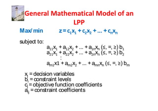
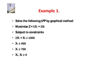
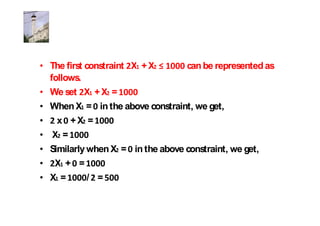
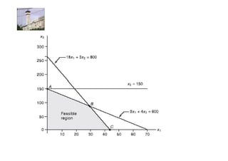
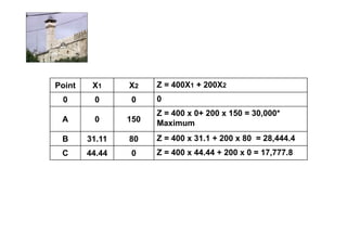
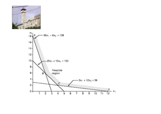
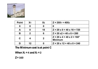
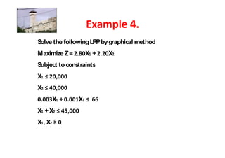
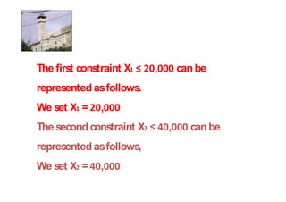
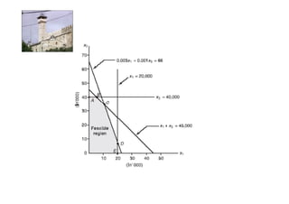
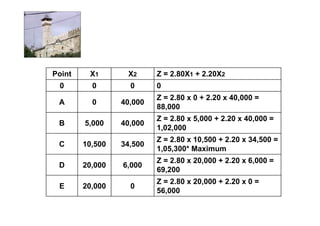
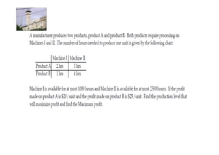
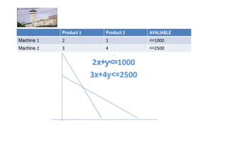
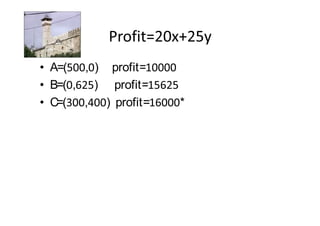
Linear programming is a technique for optimizing allocation of limited resources to activities based on constraints and an objective function. The key steps are to represent constraints graphically, identify the feasible region, and determine the optimal point that maximizes/minimizes the objective function value within the feasible region. Solving a linear programming problem graphically involves plotting the constraints and objective function on a coordinate plane and finding their intersection points.

3. Linear Programmingis a mathematical
technique for optimum allocation of limited
or scarce resources, such as labor, material,
machine, money, energy and so on , to
several competing activities such as products,
services, jobs and so on, on the basis of a
given criteria of optimality.

4. Max/ min z = c x + c x + ... + cnxn
subject to:
a x + a x + ... + a nxn ( , =, ) b
a x + a x + ... + a nxn ( , =, ) b
:
am x + am x + ... + amnxn ( , =, ) bm
xj = decision variables
bi = constraint levels
cj = objective function coefficients
aij = constraint coefficients

5. 1. Plot model constraint on a set of
coordinates in a plane
2. Identify the feasible solution space on the
graph where all constraints are satisfied
simultaneously
3. Plot objective function to find the point on
boundary of this space that maximizes (or
minimizes) value of objective function

6. Solve the following LPP by graphical method
Maximize Z = X + X
Subject to constraints
X +X
X
X
X,X

7. The first constraint X + X can be represented as
follows.
We set X + X =
When X = in the above constraint, we get,
x +X =
X =
Similarly when X = in the above constraint, we get,
X + =
X = / =

8. The second constraint X can be
represented as follows,
We set X =
The third constraint X can be
represented as follows,
We set X =

10. The constraints are shown plotted in the above figure.
Point X1 X2 Z = 5X1 +3X2
0 0 0 0
A 0 700 Z = 5 x 0 + 3 x 700 = 2,100
Z = 5 x 150 + 3 x 700 = 2,850*
B 150 700
Maximum
C 400 200 Z = 5 x 400 + 3 x 200 = 2,600
D 400 0 Z = 5 x 400 + 3 x 0 = 2,000

11. The Maximum profit is at point B
When X = and X =
Z=

12. Solve the following LPP by graphical method
Maximize Z = X + X
Subject to constraints
X + X
X + X
X
X,X

13. Solution:
The first constraint X + X can be
represented as follows.
We set X + X =
When X = in the above constraint, we get,
x + X =
X = / = .

14. Similarly when X = in the above constraint, we get,
X + x =
X = / = .

15. The second constraint X + X can be represented
as follows,
We set X + X =
When X = in the above constraint, we get,
x + X =
X = / =
X = / = .

16. Similarly when X = in the above constraint, we get,
X + x =
The third constraint X can be represented as follows,
We set X =

18. Point X1 X2 Z = 400X1 + 200X2
0 0 0 0
Z = 400 x 0+ 200 x 150 = 30,000*
A 0 150 Maximum
B 31.11 80 Z = 400 x 31.1 + 200 x 80 = 28,444.4
C 44.44 0 Z = 400 x 44.44 + 200 x 0 = 17,777.8

19. The Maximum profit is at point A
When X = and X =
Z= ,

20. Solve the following LPP by graphical method
Minimize Z = X + X
Subject to constraints
X + X
X + X
X + X
X ,X

21. The first constraint X + X can be
represented as follows.
We set X + X =
When X = in the above constraint, we get,
x + X =
X = / =

22. Similarly when X = in the above constraint, we get,
X + x =
X = / =
The second constraint X + X can be
represented as follows,
We set X + X =

23. When X = in the above constraint, we get,
x + X =
X = / =
Similarly when X = in the above constraint, we
get,
X + x =
X = / =

24. The third constraint X + X can be
represented as follows,
We set X + X =
When X = in the above constraint, we get,
x + X =
X = / =

25. Similarly when X = in the above constraint,
we get,
X + x =
X = / =

27. Point X1 X2 Z = 20X1 + 40X2
0 0 0 0
A 0 18 Z = 20 x 0 + 40 x 18 = 720
B 2 6 Z = 20 x2 + 40 x 6 = 280
Z = 20 x 4 + 40 x 2 = 160*
C 4 2
Minimum
D 12 0 Z = 20 x 12 + 40 x 0 = 240
The Minimum cost is at point C
When X = and X =
Z=

28. Solve the following LPP by graphical method
Maximize Z = . X + . X
Subject to constraints
X ,
X ,
. X + . X
X +X ,
X,X

29. The first constraint X , can be
represented as follows.
We set X = ,
The second constraint X , can be
represented as follows,
We set X = ,

30. The third constraint . X + . X can be
represented as follows, We set . X + . X =
When X = in the above constraint, we get,
. x + . X =
X= / . = ,
Similarly when X = in the above constraint, we get,
. X + . x =
X = / . = ,

31. The fourth constraint X + X , can be
represented as follows, We set X + X = ,
When X = in the above constraint, we get,
+X = ,
X = ,
Similarly when X = in the above constraint, we get,
X + = ,
X = ,

33. Point X1 X2 Z = 2.80X1 + 2.20X2
0 0 0 0
Z = 2.80 x 0 + 2.20 x 40,000 =
A 0 40,000
88,000
Z = 2.80 x 5,000 + 2.20 x 40,000 =
B 5,000 40,000
1,02,000
Z = 2.80 x 10,500 + 2.20 x 34,500 =
C 10,500 34,500
1,05,300* Maximum
Z = 2.80 x 20,000 + 2.20 x 6,000 =
D 20,000 6,000
69,200
Z = 2.80 x 20,000 + 2.20 x 0 =
E 20,000 0
56,000

34. The Maximum profit is at point C
When X = , and X = ,
Z= , ,

35. Solve the following LPP by graphical method
Maximize Z = X + X
Subject to constraints
X +X
X + X
X - X -
X X

36. The first constraint X + X can be
represented as follows.
We set X + X =
When X = in the above constraint, we get,
x +X =
X =

37. Similarly when X = in the above constraint, we get,
X + =
X = / =
The second constraint X + X can be
represented as follows,
We set X + X =

38. When X = in the above constraint, we get,
+ X =
X = / =
Similarly when X = in the above constraint,
we get,
X + x =
X =

39. The third constraint X - X - can be
represented as follows,
We set X - X = -
When X = in the above constraint, we get,
- X =-
X =- / = .
Similarly when X = in the above constraint, we get,
X x =-
X =-

41. Point X1 X2 Z = 10X1 + 8X2
0 0 0 0
A 0 7.5 Z = 10 x 0 + 8 x 7.5 = 60
B 3 9 Z = 10 x 3 + 8 x 9 = 102
C 6 8 Z = 10 x 6 + 8 x 8 = 124* Minimum
D 10 0 Z = 10 x 10 + 8 x 0 = 100
The Maximum profit is at point C
When X = and X =
Z=

45. Product Product AVALIABLE
Machine <=
Machine <=
x+y<=
x+ y<=

46. A=( , ) profit=
B=( , ) profit=
C=( , ) profit= *

47. Click on Tools
to invoke Solver.
Objective function
=E -F
=E -F
=C *B +D *B
=C *B +D *B
Decision variables bowls
(x )=B ; mugs (x )=B
Copyright John Wiley &
Supplement -
Sons, Inc.

48. After all parameters and constraints
have been input, click on Solve.
Objective function
Decision variables
Decision variables
C *B +D *B
C *B +D *B
Click on Add to
insert constraints
Copyright John Wiley &
Supplement -
Sons, Inc.

49. Copyright John Wiley &
Supplement -
Sons, Inc.